Revised, March 2002.
Inequality and Economic Growth: Do Natural Resources Matter?
by
Thorvaldur Gylfason* and Gylfi Zoega**
Abstract
This paper is intended to demonstrate, in theory as well as empirically, how increased dependence on natural resources tends to go along with less rapid economic growth and greater inequality in the distribution of income across countries. On the other hand, public policy in support of education can simultaneously enhance equality and growth by raising the return to working in higher technology (that is, nonprimary) industries and thus counter some of the potentially adverse effects of excessive natural resource dependence. Together, these two variables – natural resources and education – can help account for the inverse relationship between inequality and growth observed in cross-country data. Moreover, the analysis highlights the role of public revenue policy. Taxes and fees can be used to reduce the attractiveness of primary-sector employment, lift the marginal productivity of capital in higher technology industries and thus increase the rate of interest and economic growth, while reducing the inequality of income and wealth. * Research Professor of Economics, University of Iceland; Research Fellow, CEPR and CESifo; and Research Associate, SNS – Swedish Center for Business and Policy Studies, Stockholm. Mail Address: Faculty of Economics and Business Administration, University of Iceland, 101 Reykjavik, Iceland. Phone: 354-525-4533/4500. Fax: 354-552-6806. E-mail: [email protected]. This paper was prepared for a CESifo Conference on Growth and Inequality, held in Bavaria 18-19 January 2002. Financial support from Jan Wallanders och Tom Hedelius Stiftelse in Sweden is gratefully acknowledged. ** Senior Lecturer in Economics, Birkbeck College; Research Affiliate, CEPR; and Fellow, Institute of Economic Studies, University of Iceland. Mail Address: Department of Economics, Birkbeck College, University of London, 7-15 Gresse Street, London W1P 2LL, United Kingdom. Phone: 44-207-631-6406. Fax: 44-207-631-6416. E-mail: [email protected]. Helpful comments from Theo Eicher, Stephen Turnovsky and other conference participants are acknowledged with thanks.
1. Introduction For a long time, many economists were of the view that economic efficiency and
social equality were essentially incompatible, almost like oil and water. The perceived
but poorly documented trade-off between efficiency and equality was commonly
regarded as one of the main tenets of modern welfare economics. One of the key ideas
behind this perception was that increased inequality could increase private as well as
social returns to investing in education and exerting effort in the hope of attaining a
higher standard of life. Redistributive policies were supposed to thwart these
tendencies and blunt incentives by penalizing the well off through taxation and by
rewarding the poor. Economic efficiency – both static and dynamic – was bound to
suffer in the process, or so the argument went.
More often than not in recent empirical work, measures of income inequality have
turned out to have a negative effect on economic growth across countries. Thus
Alesina and Rodrik (1994), Persson and Tabellini (1994) and Perotti (1996) report
that inequality hurts growth. Barro (2000) assesses the relationship between economic
growth and inequality in a panel of countries over the period from 1965 to 1995 and
finds – by studying the interaction of the Gini index and the initial level of income in
a growth regression – that increased inequality tends to retard growth in poor
countries and boost growth in richer countries.1 However, Barro finds no support for a
relationship between inequality and growth in his sample as a whole. Forbes (2000)
finds that the relationship between inequality and growth becomes positive in a
pooled regression when country effects are included. She claims that country-specific,
time-invariant, omitted variables generate a significant negative bias in the estimated
coefficients reflecting the effects of inequality on growth in pure cross sections and
mentions corruption and the level of public education as two candidates in this regard.
Banerjee and Duflo (2000b) claim that this result is misleading, and arises from
imposing a linear structure on highly nonlinear data.
The above-mentioned empirical results – showing, by and large, that rapid
economic growth tends to go along with less, not more, inequality – call for an
explanation. Thus far, the explanations on offer involve showing how inequality
1 This empirical finding does not support the claim of Garcia-Peñalosa (1995) that in rich countries increased inequality discourages education and growth by increasing the number of poor people who cannot afford education whereas in poor countries increased inequality encourages education and growth by increasing the number of rich people who can afford education.
1

affects growth either directly or indirectly through its effects on public policy,
including taxes and transfers and education expenditures. We will now briefly
describe some of these theories before returning to our proposed thesis, which
involves natural resources as a joint determinant of both inequality and growth.
First, large inequalities of income and wealth may trigger political demands for
transfers and redistributive taxation. To the extent that transfers and taxation distort
incentives to work, save and invest, inequality may impede growth. It is not clear,
however, that this type of political-cum-fiscal explanation necessarily implies an
inverse relationship between inequality and growth, for it is possible that during the
redistribution phase increased equality and a drop in growth go hand in hand,
especially in panel data that reflect developments over time country by country as
well as cross-sectional patterns. Perotti (1996) finds little empirical support for this
type of explanation. Moreover, in democratic countries with an unequal distribution
of income and with many poor people, the electorate may vote for more and better
education as well as higher taxes and transfers (Saint-Paul and Verdier, 1993, 1996),
thus obscuring the relationship between inequality and growth. Absent democracy,
dictators may still find it in their own interest to redistribute incomes and reform
education in order to promote social peace and strengthen their own hold on political
power (Alesina and Rodrik, 1994). Easterly and Rebelo (1993) report empirical
results that suggest that increased inequality is associated with both higher taxes and
more public expenditure on education in a large sample of countries in the period
1970-1988.
In second place, the initial extent of inequality probably makes a difference. An
equalization of incomes and wealth in countries with gross inequities, such as Brazil
where the Gini index is 60, would seem likely to foster social cohesion and peace and
thus to strengthen incentives rather than weaken them, whereas in places like
Denmark and Sweden, where the Gini index is 25 and incomes and wealth are thus
already quite equitably distributed by world standards, further equalization might well
have the opposite effect. Excessive inequality may be socially divisive and hence
inefficient: it may motivate the poor to engage in illegal activities and riots, or at least
to divert resources from productive uses, both the resources of the poor and those of
the state. Social conflict over the distribution of income, land or other assets can take
place through labor unrest, for instance, or rent seeking which can hinder investment
2

and growth (Benhabib and Rustichini, 1996).2 Alesina and Perotti (1996) report
empirical evidence of an inverse relationship between inequality and growth through
socio-political instability.3
Third, national saving may be affected by inequality if the rich have a higher
propensity to save than the poor (Kaldor, 1956). In this case inequality may be good
for growth in that the greater the level of inequality, the higher is the saving rate and
hence also investment and economic growth. Against this Todaro (1997) suggests that
the rich may invest in an unproductive manner – count their yachts and expensive
cars. Barro (2000) finds no empirical evidence of a link between inequality and
investment.
Fourth, increased inequality may hurt education rather than helping it as suggested
by the political-economy literature referred to at the beginning of this brief discussion.
If so, increased inequality may hinder economic growth through education. Galor and
Zeira (1993) and Aghion (1998) argue that this outcome is likely in the presence of
imperfect capital markets. If each member of society has a fixed number of
investment opportunities, imperfect access to credit and a different endowment of
inherited wealth, the rich would end up using many of their investment opportunities
while the poor could only use a few. Therefore, the marginal return from the last
investment opportunity of the rich would be much lower than the marginal return of
the last investment opportunity of the poor. Redistribution of wealth from the rich to
the poor would increase output because the poor would then invest in more productive
projects at the margin. This argument can also be applied to investment in human
capital if we assume diminishing returns to education. In this case, taking away the
last few quarters of the university education of the elite and adding time to the more
elementary education of the poor would raise output and perhaps also long-run
growth, other things being the same. Income redistribution would reverse the decline
in investment in human capital resulting from the credit-market failure.4
The distribution of income and wealth may also affect the amount of public and
private investment in education. When a large part of the population is poor, it may be
more likely that the majority of voters will support expenditures on public education
2 Further, Aghion (1998) suggests that excessive inequality may be associated with macroeconomic volatility through credit cycles because of unequal access to credit and thus to investment opportunities, and that this may hurt investment and growth. 3 See also Aghion, Caroli and Garcia-Peñalosa (1999). 4 For a further discussion of recent empirical literature on inequality and growth, see Bénabou (1996).
3
aimed at the poor, as argued by Saint-Paul and Verdier (1993, 1996) and corroborated
empirically by Easterly and Rebelo (1993), but the effect could also, in principle, go
the other way. If so, the more deprived and detached from the mainstream population
is the poorer segment, the less likely the poor are to participate in or affect the
outcome of elections. As a result the general level of education may suffer – the more
so, the more capital-constrained is the poorer segment of the population. A virtuous
circle may arise when redistribution of income leads to an increase or improvement in
human capital, which then induces voters to prefer higher expenditures on education,
which again pulls more workers out of poverty, and so on. At an empirical level, we
would expect increased equality to enhance economic growth through its effect on
education, and vice versa. That is, more and better general education may be expected
to reduce public tolerance against extreme inequality and thus to reduce inequality
through the political process, thereby stimulating economic growth. These processes
can be mutually reinforcing; that is, if increased social equality encourages education
and economic growth, this does not mean that more and better education cannot
similarly, and simultaneously, enhance equality and growth.
The models reviewed above all have the same basic structure: inequality affects
some unknown intermediate variable X which, in turn, makes a difference for
economic growth. In this paper we take a different approach: we view both economic
growth and inequality of incomes as well as of educational attainment and of land as
endogenous variables and argue that the inverse relationship between inequality and
growth does not imply causality one way or the other. We propose an explanation
which, in contrast to the ones surveyed in the literature reviewed briefly above,
involves a variable that is exogenous to most economic models. This variable is the
abundance of, or rather dependence on, natural resources, which we measure by the
amount of natural capital per person and the share of natural capital in national
wealth, respectively. We will argue, on theoretical grounds as well as empirically, that
a direct relationship between natural resource intensity and inequality, on the one
hand, and between natural resource intensity and growth, on the other hand, can help
account for the inverse cross-sectional relationship between inequality and growth
that is observed in the data, assuming that natural resources are given. The first
relationship – between natural resource intensity and inequality – was documented by
Bourguignon and Morrison (1990) in a sample of 35 developing countries in 1970,
while the second relationship – between natural resource intensity and growth – has
4

been scrutinized by a number of authors in recent years, beginning with Sachs and
Warner (1995). Moreover, we assume that the ownership of natural resources tends to
be less equally distributed than other assets within as well as across countries. To the
extent that this is not the case at the outset, we assume that rent seeking and other
forces, frequently compounded by a lack of democracy, will see to it that the natural
resources end up in the hands of a relatively small minority – a military regime, say,
or a royal family.
The paper proceeds as follows. In Section 2, we set out our view of the way in
which natural resources can affect inequality and growth. In Section 3, we describe
the data that we use to measure income inequality and also gender inequality in
education; we also discuss inequality in the distribution of land. In Section 4, we
present simple cross-country correlations between three different measures of
education, three different measures of inequality and economic growth, and thus
allow the data to speak for themselves. In Section 5, we attempt to dig a little deeper
and report the results of cross-sectional multiple regression analysis where growth is
traced to natural resource intensity, education and inequality as well as to other factors
commonly used in growth regression analysis (investment and initial income), and
where some of the determinants of growth, including education and inequality, are
explicitly modeled as endogenous variables. Section 6 concludes the discussion.
2. Resources, distribution and growth An important potential weakness of the many stories purporting to explain the
relationship between inequality and growth is that both of these variables are
endogenous. This leaves open the possibility that a third, exogenous variable is
affecting both, thus giving rise to the inverse correlation between the two.
Specifically, a country’s abundance of, or dependence on, natural resources can under
many circumstances be viewed as exogenous to models of economic growth and also
to models attempting to explain the extent of income inequality. But even if we treat
natural resources as exogenous, we are aware that both natural resource extraction and
reserves can respond to economic forces; for example, oil prices can influence oil
production as well as oil exploration. We do not address this problem in this paper,
but we acknowledge its potential importance; at some point, this problem will need to
be addressed. Here we want to let it suffice to explore the possibility that natural
5
resource ownership impinges on both inequality and growth and thus illuminates the
inverse relationship between inequality and growth that has been observed in cross-
sectional data.
We will now show how natural resource dependence is inversely related to both
equality and growth in a standard growth model. Thereafter, we will test this
prediction empirically in a sample of 87 industrial and developing countries in the
period 1965-1998. Our theoretical model can be summarized as follows: workers can
earn a living by either working in the primary sector extracting natural resources from
the soil or the sea or through paid employment in the manufacturing sector, including
services. Because human capital is equally spread across the population, wage income
in manufacturing is the same for all workers. However, due to the whims of nature, or
the competition for the rent generated by the natural resource, earnings in the primary
sector are unequal at each point in time. It follows that the more time workers devote
to natural resource extraction, the more unequal the distribution of income. And
growth is also affected. If we assume, quite plausibly, that the manufacturing industry
provides greater opportunities for learning and innovation, it follows that the more
time workers spend in the primary sector, the lower will be the rate of growth. Hence,
abundant natural resources cause both inequality and slow growth by tempting
workers away from industries where technology and output are more likely to
progress and grow and where earnings are more equally shared. Elsewhere (Gylfason
and Zoega, 2001b) we show how saving and investment – and hence also growth –
can depend inversely on natural resources. The intuition is again straightforward:
when physical capital is less important in the production technology, the optimal rate
of saving is lower. Therefore, the optimal level of steady-state capital is lower. If we
now postulate learning-by-investing (as in Romer, 1986), the rate of technological
progress and the rate of growth of output per capita will consequently both be lower.
Our hypothesis has the advantage that here we have an exogenous variable that
affects the two endogenous variables in a predictable way, and this makes any
empirical testing of the theory more robust. We will show how the relationship
between inequality and growth can arise in the presence of natural resources. If
natural resources affect both inequality and growth, then this could shed new light on
the statistical relationship between inequality and growth. But to do this we need to
identify, on theoretical grounds as well as empirically, the relationship between
natural resources and inequality, on the one hand, and between natural resources and
6
growth, on the other hand. It is to this task that we now turn.
2.1 Allocation of time
Imagine a world in which natural resources generate a constant flow of riches. All one
has to do is go out and pick the fruits of nature, be they diamonds, fish or oil. This
could involve passively standing beneath an apple tree or a coconut palm and picking
up the fruits that fall to the ground or one could have to exert oneself looking for
fruits, diamonds or fish, to take a few examples. The value of each bundle of the
natural resource is equal to R and the likelihood of finding a bundle increases with the
time spent searching. Now imagine that amidst the bounties of nature there is a
manufacturing industry that uses labor and capital to produce output without using or
depending in any way on the natural resource. Assume, crucially for our argument,
that workers face a more challenging and stimulating work environment in the
manufacturing industry, because manufacturing is more likely to foster learning and
innovation. In particular, assume that there is learning-by-investing in manufacturing.
Workers have a choice when it comes to their work effort: they can spend part of
or all of their time trying their luck picking fruits or they can take a paid job in
industry. Each individual has to decide how much time to spend picking fruits and
how much time to spend in paid employment. We denote the fraction of time spent in
productive employment by β and the fraction spent picking fruits by 1-β.
Now assume that the discovery of a bundle of natural resources valued R is a
random event and follows a Poisson distribution. Denote the number of such
discoveries by the random variable N. The random event is then defined as “a worker
finds a bundle of the natural resource during a unit of time” and has the following
density:
(1) ( )( ) ( )[ ]
!11
NeNf
Nβγβγ −=−−
for N = 0, 1, 2 …
where the mean arrival rate – that is, the expected number of discoveries by a given
worker or, equivalently, the probability that a discovery will be made by the worker
within a unit of time – is ( ) ( )βγ −= 1NE . The expected number of discoveries for the
representative individual is thus a linear function of the fraction of time spent
searching. The larger the share of time spent in nature, the more bundles will be
discovered. The parameter γ measures search effectiveness.
7
There are L individuals (identical by assumption) spending part of their time
searching. The aggregate income from the natural resource is then
(2) Y NLRn =
The expected value and the variance of N given by the Poisson distribution are both
equal to ( )βγ −1 . Since all individuals are identical, it follows that the variance
across the population in the number of discoveries of the natural resource bundles per
unit of time is also equal to ( )βγ −1 . We now have the following result: the variance
of the distribution of income emanating from the natural resource is an increasing
function of the time devoted by each worker to the natural-resource-based sector –
primary sector, for short. Define income per capita by lower case letters. We then
have
(3) ( ) ( ) ( ) ( )RyRyE nn βγβγ −=−= 1var,1
The expected per capita income or rent from the natural resource as well as the
variance of this per capita income across the population of workers is an increasing
function of the abundance of the resource R and also an increasing function of the
time spent procuring it 1-β.
We now turn to the manufacturing industry, which offers workers an alternative to
wandering around nature. This industry uses capital and labor to produce output and
offers opportunities for learning and innovation. The production function is
(4) Y q ( ) ( )1i i iK K Lα αβ −=
Here q denotes the quality of capital and takes a value between zero and one,5 Ki and
Li denote the capital and labor used by firm i and K is the aggregate capital stock in
5 Like Scott (1989), we distinguish between quantity and quality. If some investment projects miss the mark and fail to add commensurately to the capital stock, we have q < 1. There are three ways to interpret q: (a) as an indicator of distortions in the allocation of installed capital due to a poorly developed financial system, trade restrictions or government subsidies that attract capital to unproductive uses in protected industries or in state-owned enterprises where capital may be less productive than in the private sector (Gylfason, Herbertsson and Zoega, 2001); (b) as the ratio of the economic cost (i.e., minimum achievable cost) of creating new capital to the actual cost of investment (Pritchett, 2000) – that is, K is then measured on the basis of actual costs, which may overstate its productivity; or (c) as a consequence of aging: the larger the share of old capital in the capital stock currently in operation, i.e., the higher the average age of capital in use, the lower is its overall quality (Gylfason and Zoega, 2001a). For our purposes, the three interpretations are analytically equivalent. However, we assume that the quality of capital has remained constant in the past, which means that all units of capital are of the same quality. In other words, we are not interested here in the implications of
8

the manufacturing sector. As in Romer (1986) the aggregate capital stock is a proxy
for the accumulated knowledge that has been generated in the past through investment
at all firms. This is what sets manufacturing apart from the primary sector; it uses
capital and the installation of new units of capital generates a flow of ideas that raises
productivity in a labor-augmenting fashion. In contrast, the primary sector does not
offer similar opportunities for learning and innovation.
We assume a perfectly competitive market for labor and capital. Assuming
symmetric equilibrium, so that K=kL, gives the following first-order conditions for
maximum profit, and also for equilibrium in the two factor markets:
(5) ( ) ( ) wLkqdLdY
i
i ββα αα =−= −11
(6) ( ) δβα αα +== − rLqdKdY
i
i 1
where w is the real wage, r is the real interest rate and δ is the rate at which installed
capital loses its usefulness over time, as a result of economic obsolescence as well as
physical wear and tear (Scott, 1989).6
The representative worker/consumer has to make two decisions each moment of
his infinite life. He has to decide how much to consume and save and how much time
to spend working in the manufacturing sector rather than trying his luck in the
primary sector. We assume that he cannot do both at the same time. Hence a decision
to spend more time in the primary sector causes him to spend less time in paid
employment making manufactures. Moreover, we assume that time spent in the
primary sector is costly: a direct cost η is incurred for each moment spent. Finally,
there is a tax on wages tw and also a tax on income from the natural resources tn.
The worker maximizes the discounted sum of future utility from consumption:
(7) max ( )∫∞
−
0
log,
dtecc
tt
ρ
β
where ρ is the discount rate, subject to
having different vintages of capital. 6 The parameters q and δ can both be modeled as endogenous choice parameters (as in Gylfason and Zoega, 2001a), but here we treat them as exogenous magnitudes for simplicity, even if we acknowledge that depreciation may depend on quality, through obsolescence.
9
( ) ( ) ( ) ( ) tnwtt ctRtwraa −−−−−+−+= ηβγβγβ 1111�
By assumption, the worker does not gain any utility (or suffer disutility) in the
primary sector, nor from being employed. The worker has assets a, which he
accumulates if his earnings exceed expenditures (henceforth, we omit time
subscripts). His earnings come from three sources: There is interest income on assets
ra which is tax-free, there is wage income from employment βw, taxed at tw, and there
is the value of the primary goods he picks or produces (1-β)R, taxed at tn. The worker
then incurs the direct cost η and consumes c per unit of time. A necessary condition
for optimal consumption is
(8) 1λ
=c
where λ denotes the shadow price of wealth. Consumption is at an optimum when the
marginal utility of consumption is equal to the shadow price of wealth at each instant.
More interesting is equation (9), which helps determine the optimal allocation of time:
(9) ( ) ( ) ηγ −−=− nw tRtw 11
The left-hand side of equation (9) shows the marginal benefit from working longer in
manufacturing net of taxes, while the right-hand side shows the marginal benefit from
fruit picking, also net of taxes. While each worker takes wages w as given, wages do
nevertheless respond to market forces. Combining equations (5) and (9) gives the
following equation:
(10) ( ) ( ) ( ) ηγβα ααα −−=−− −−nw tRtLkq 111 1
Solving for β gives
(11) ( ) ( )( )
ααα
ηγαβ
11
111
−−
−−=−
n
w
tRtLkq
The time spent in industrial employment β is decreasing in the value of the natural
resource R and search effectiveness γ as well as in taxes on wage income tw, and
increasing in the accumulated knowledge in the manufacturing industry kL (=K), the
productivity of capital q, taxes on natural resources tn and the cost of utilizing the
natural resource η.
10

2.2 Work and growth
We can now describe the various ways in which natural resources affect the allocation
of labor in our model.
• The discovery of natural resources R raises the reward to producing primary
output and reduces the optimal time spent in manufacturing.
• A decrease in the cost of producing primary output η and an increase in search
effectiveness γ have an effect identical to that of a resource discovery: labor leaves
manufacturing for the primary sector.
• The structure of the tax system affects the allocation of time. The higher are taxes
on wages tw and the lower are taxes on income or rent from natural resource
extraction tn, the more time is devoted to producing primary goods.
• History matters because past learning-by-investing in the industrial sector
determines current knowledge as reflected by k and hence also real wages. The
more advanced the manufacturing sector, the higher the wages it can afford to pay
and the more time workers spend in manufacturing.
The last point explains why natural resource abundance and dependence do not
have to go together. Abundance of natural resources is a significant impediment to
growth only if productivity and wages in the manufacturing sector are low, that is, if
there is little accumulated knowledge and expertise in the sector. But the presence of
abundant natural resources can prevent manufacturing from “taking off”, thereby
preventing innovation and learning from taking place:
• When R is sufficiently high, or when productivity in the manufacturing sector is
sufficiently low, it can be optimal not to spend any time in manufacturing. In this
case, growth never takes off.
Education provides a possible solution to this dilemma by increasing labor
productivity in manufacturing:
• Education can increase knowledge, and thereby also labor productivity which, like
past learning-by-doing, lifts wages and draws workers to the manufacturing
industry from the primary sector.
We now turn to the remaining necessary condition for maximum utility, the Euler
equation giving optimal growth of consumption:
(12) ρ−= rcc�
11
Equations (6) and (12) give the optimal rate of growth of consumption and output:
(13) ( ) ρδβα αα −−= −1Lqg
Growth is an increasing function of β, the share of time spent producing manufactures
rather than primary goods.
There are two market failures in the model. The first is the standard one that firms,
when investing, neglect the gains from learning and knowledge spillovers to other
firms. In contrast, a social planner uses the average product of capital – not the private
marginal product – to measure the cost of capital. Second, workers compare the
current benefit from spending time in the two sectors but ignore the growth effect of
industrial employment: by spending more time in the manufacturing industry they,
collectively, would raise the marginal product of capital, the interest rate and
economic growth. This makes their wages grow more rapidly. By withdrawing labor
from the primary sector, workers would invest in a higher future wage. However, each
worker has only a very small effect on growth imparting an external benefit to others.
We can now summarize the relationship between natural resources and growth.
• A rise in the natural resource rent R attracts more people to the primary sector in
the hope of securing a piece of the action. These people leave the manufacturing
sector, thereby lowering the private marginal product of capital, the rate of interest
and the rate of growth of consumption and output. This is the Dutch disease
working through the labor market (Paldam, 1997).
• When abundant natural resources reduce the incentive to provide good education
(Gylfason, 2001), this reduces labor productivity and wages, hence reinforcing the
incentive to stay in the natural resource sector. An abundant natural resource – a
high value of R – attracts workers and this effect is reinforced by bad education
which drives people away from industrial employment.
• If natural resources reduce the quality of society’s institutions, this could manifest
itself in a reduction in the private cost of rent seeking η. Moreover, less developed
capital markets are likely to generate a lower quality capital stock q, which
depreciates at a higher rate δ (Gylfason and Zoega, 2001a, 2001b).
We can now combine these insights with the earlier result showing that the
variance of income or rent emanating from the natural resource sector is
12

(14) ( ) ( )Ryn βγ −= 1var
Equations (13) and (14) show that while economic growth is increasing in β,
inequality – measured by the variance of income – is decreasing in β. According to
our thesis, any variable that increases the value of β is likely to stimulate growth and
reduce inequality. Equation (11) shows that an abundance of natural resources –
relative to the level of technological know-how – will lower the value of β. In
contrast, any variable that raises labor productivity and wages in the manufacturing
sector will raise β, increase growth and reduce inequality. The knowledge that has
been generated through past investment and production is one such factor. Another
factor is the level of education. Education that raises productivity and wages in
industry will discourage workers from spending time in the natural resource sector
and hence raise growth and reduce inequality. At last, the tax system can affect
growth and equality: a high tax on natural resource rents and a low tax on wages
increases the value of β, hence raising growth and reducing inequality.
3. Measuring inequality In what follows, we make use of three different measures of inequality. Take income
inequality first. The Gini index measures the extent to which income (or, in some
cases, consumption) among individuals or households within an economy deviates
from a perfectly equal distribution. A Gini index of zero represents perfect equality,
while a Gini index of 100 means perfect inequality. As Figure 1 shows, the Gini index
is closely correlated with the log of the ratio of the income or consumption of the 20
percent of households with the highest incomes to the income or consumption of the
20 percent of households with the lowest incomes (the “20/20 ratio”). In our sample,
the 20/20 ratio is lowest (2.6, Gini = 19.5) in the Slovak Republic and highest in
Sierra Leone (57.6, Gini = 62.9). The regression line through the scatter in Figure 1
shows that each ten-point increase in the Gini index goes along with roughly a
doubling of the 20/20 ratio. Thus, for example, the Nordic countries have a Gini index
of 25 and a 20/20 ratio of 3 whereas the United Kingdom has a Gini index of 35 and a
20/20 ratio of 6. The corresponding figures are 30 and 4 for Germany and 40 and 8 for
the United States as well as for China and Russia. The data come from nationally
representative household surveys and refer to different years between 1983-85 and
13
1998-99 (World Bank, 2000, Table 2.8). The data refer to either (a) personal or
household incomes before taxes and transfers or (b) consumption expenditures and,
hence, implicitly incomes after taxes and transfers. Whenever possible, consumption
was used rather than income (same source). The Gini index of income inequality is
available for 75 of the 87 countries in our sample.
Our second inequality measure is intended to reflect one aspect of social
inequality, that is, the unequal access of males and females to education. We take the
difference between the average secondary-school enrolment rates of males and
females in 1980-1997 to represent gender inequality in education. In a majority of
cases where the rates are different, more males than females go to secondary school.
In some cases, however, more females than males attend secondary schools. Even so,
we use the arithmetic rather than absolute difference between male and female
enrolment rates as our inequality measure. This means that we view a change from a
situation where, say, the secondary-school enrolment rate for males is 17 percentage
points higher than that for females (as in Egypt) to a situation where the secondary-
school enrolment rate for females is 17 percentage points higher than that for males
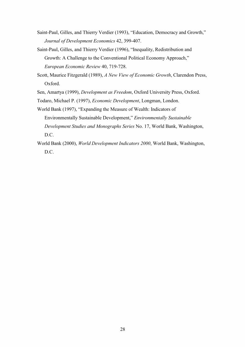
(as in Finland) as a decrease in gender inequality. Surprisingly, Figure 2 shows that
there is in our sample no discernible correlation between income inequality as
measured by the Gini index and gender inequality of education as measured by the
excess of male over female secondary-school enrolment. Thus economic and social
inequality, as measured here, do not necessarily go hand in hand.
Our cross-country data support the notion of a Kuznets curve: income inequality
tends to increase with income at low levels of income and to decrease with income at
higher levels of income, as shown in Figure 3. Galor and Moav (1999) suggest the
following interpretation of the Kuznets curve: in early stages of development, when
investment in physical capital is the main engine of economic growth, inequality
spurs growth by directing resources towards those who save and invest the most,
whereas in more mature economies human capital accumulation takes the place of
physical capital accumulation as the main source of growth, and inequality impedes
growth by hurting education because poor people cannot fully finance their education
in imperfect credit markets. On the other hand, the gender inequality of education
varies inversely and linearly with initial income, without any visible tendency for
gender inequality to increase with income at low levels of income (Figure 4).
The third measure of inequality that we will use is the Gini index for the
14

distribution of land. This measure is taken from Deininger and Olinto (2000), and
covers 50 of the 87 countries in our sample. Figure 5 shows that, almost without
exception, land is less equally distributed than income in our sample. Spearman’s rank
correlation between the two measures is 0.57.
4. Cross-country patterns in the data
In this section, we allow the data to speak for themselves in the form of a series of
bivariate cross-sectional correlations. We first take a look at the correlations between
our three measures of inequality and economic growth, all of which are
unambiguously negative in our data: greater inequality in the distribution of income
and land as well as in access to education tends to go together with lower rates of
growth. We then move on to show that two of the three measures of inequality
increase from country to country in tandem with the share of natural capital in
national wealth. This opens up the possibility that it is the variation in natural capital
in the sample that generates the apparent relationship between inequality and growth:
when natural resources become more important, inequality rises and growth recedes.
This was the prediction of our model in Section 2. At last, we also show that income
inequality and three different measures of education are inversely related, while
education and growth are positively correlated. This finding accords with earlier
research indicating that education, by reducing inequality and fostering growth, can
help clarify the inverse relationship between inequality and growth that is observed in
the data. Unlike natural resource abundance, however, education is probably best
viewed as an endogenous variable, a possibility that we address explicitly in the
regression analysis presented in Section 5.
4.1 Inequality and growth
Let us now begin by looking at the cross-country pattern of income inequality and
economic growth. Figure 6 shows a scatterplot of the annual rate of growth of gross
national product (GNP) per capita from 1965 to 1998 (World Bank, 2000, Table 1.4)
and the inequality of income or consumption as measured by the Gini index (same
source, Table 2.8). The growth rate has been adjusted for initial income: the variable
on the vertical axis is that part of economic growth that is not explained by the
country’s initial stage of development, obtained as a residual from a regression of
15

growth during 1965-1998 on initial GNP per head (i.e., in 1965) as well as the share
of natural capital in national wealth, taken from World Bank (1997). The 75 countries
shown in the figure are represented by one observation each.7 The regression line
through the scatterplot suggests that an increase of about 12 points on the Gini scale
from one country to another is associated with a decrease in per capita growth by one
percentage point per year on average. Twelve points on the Gini scale correspond
roughly to the difference between income inequality in the United Kingdom (Gini =
36) and in Sweden and Japan (Gini = 25). The relationship in Figure 6 is statistically
significant (Spearman’s rank correlation is -0.50). If rich countries and poor are
viewed separately, a similar pattern is observed in both groups (not shown). Shaving
one percentage point off any country’s annual growth rate is a serious matter because
the (weighted) average rate of per capita growth in the world economy since 1965 has
been about 1½ percent per year. We see no signs of the positive cross-sectional
relationship between inequality and growth in rich countries reported by Barro (2000),
nor do we see any evidence of the nonlinearity in the panel relationship documented
by Banerjee and Duflo (2000a, 2000b).
Figures 7 and 8 tell a similar story. Here we see the cross-country pattern of per
capita growth as measured in Figure 6 and gender inequality of education (Figure 7)
and land inequality (Figure 8). The pattern is not as clear as in Figure 6, but it is still
statistically significant (Spearman’s rank correlation is -0.32 and -0.37, respectively).
The number of countries is 75 and 50 in the two figures. All countries for which the
requisite data are available are included in all the figures in the paper, without
exception.
4.2 Natural resources, inequality and growth
In Figure 9, we measure natural resource dependence by the share of natural capital in
national wealth in 1994 – i.e., the share of natural capital in total capital, which
comprises physical, human and natural capital (though not social capital; see World
Bank, 1997). The natural capital variable is intended to come closer to a direct
measurement of the intensity of natural resources across countries than the various
7 All countries for which the requisite data are available are included in all the figures in the paper, without exception.
16
proxies that have been used in earlier studies, mainly the share of primary (i.e., non-
manufacturing) exports in total exports or in gross domestic product (GDP) and the
share of the primary sector in employment or the labor force. The latter proxies may
be prone to bias due to product and labor market distortions.
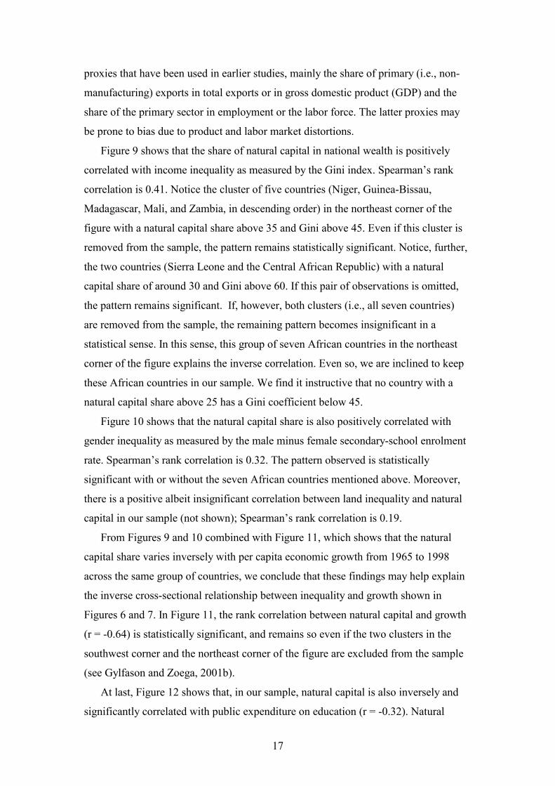
Figure 9 shows that the share of natural capital in national wealth is positively
correlated with income inequality as measured by the Gini index. Spearman’s rank
correlation is 0.41. Notice the cluster of five countries (Niger, Guinea-Bissau,
Madagascar, Mali, and Zambia, in descending order) in the northeast corner of the
figure with a natural capital share above 35 and Gini above 45. Even if this cluster is
removed from the sample, the pattern remains statistically significant. Notice, further,
the two countries (Sierra Leone and the Central African Republic) with a natural
capital share of around 30 and Gini above 60. If this pair of observations is omitted,
the pattern remains significant. If, however, both clusters (i.e., all seven countries)
are removed from the sample, the remaining pattern becomes insignificant in a
statistical sense. In this sense, this group of seven African countries in the northeast
corner of the figure explains the inverse correlation. Even so, we are inclined to keep
these African countries in our sample. We find it instructive that no country with a
natural capital share above 25 has a Gini coefficient below 45.
Figure 10 shows that the natural capital share is also positively correlated with
gender inequality as measured by the male minus female secondary-school enrolment
rate. Spearman’s rank correlation is 0.32. The pattern observed is statistically
significant with or without the seven African countries mentioned above. Moreover,
there is a positive albeit insignificant correlation between land inequality and natural
capital in our sample (not shown); Spearman’s rank correlation is 0.19.
From Figures 9 and 10 combined with Figure 11, which shows that the natural
capital share varies inversely with per capita economic growth from 1965 to 1998
across the same group of countries, we conclude that these findings may help explain
the inverse cross-sectional relationship between inequality and growth shown in
Figures 6 and 7. In Figure 11, the rank correlation between natural capital and growth
(r = -0.64) is statistically significant, and remains so even if the two clusters in the
southwest corner and the northeast corner of the figure are excluded from the sample
(see Gylfason and Zoega, 2001b).
At last, Figure 12 shows that, in our sample, natural capital is also inversely and
significantly correlated with public expenditure on education (r = -0.32). Natural
17
capital is also inversely and significantly related to years of schooling for girls and
secondary-school enrolment for both genders (not shown).
4.3 Inequality and education
Let us now consider the three above-mentioned measures of education inputs,
outcomes and participation and how they vary with inequality and economic growth.
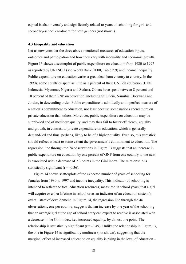
Figure 13 shows a scatterplot of public expenditure on education from 1980 to 1997
as reported by UNESCO (see World Bank, 2000, Table 2.9) and income inequality.
Public expenditure on education varies a great deal from country to country. In the
1990s, some countries spent as little as 1 percent of their GNP on education (Haiti,
Indonesia, Myanmar, Nigeria and Sudan). Others have spent between 8 percent and
10 percent of their GNP on education, including St. Lucia, Namibia, Botswana and
Jordan, in descending order. Public expenditure is admittedly an imperfect measure of
a nation’s commitment to education, not least because some nations spend more on
private education than others. Moreover, public expenditure on education may be
supply-led and of mediocre quality, and may thus fail to foster efficiency, equality
and growth, in contrast to private expenditure on education, which is generally
demand-led and thus, perhaps, likely to be of a higher quality. Even so, this yardstick
should reflect at least to some extent the government’s commitment to education. The
regression line through the 74 observations in Figure 13 suggests that an increase in
public expenditure on education by one percent of GNP from one country to the next
is associated with a decrease of 2.3 points in the Gini index. The relationship is
statistically significant (r = -0.36).
Figure 14 shows scatterplots of the expected number of years of schooling for
females from 1980 to 1997 and income inequality. This indicator of schooling is
intended to reflect the total education resources, measured in school years, that a girl
will acquire over her lifetime in school or as an indicator of an education system’s
overall state of development. In Figure 14, the regression line through the 46
observations, one per country, suggests that an increase by one year of the schooling
that an average girl at the age of school entry can expect to receive is associated with
a decrease in the Gini index, i.e., increased equality, by almost one point. The
relationship is statistically significant (r = -0.49). Unlike the relationship in Figure 13,
the one in Figure 14 is significantly nonlinear (not shown), suggesting that the
marginal effect of increased education on equality is rising in the level of education –
18

that is, there may be increasing returns to schooling in terms of equality. Sen (1999),
among others, emphasizes the importance of educating girls in developing countries.
The corresponding relationship for males (not shown) is virtually the same as for
females.
In Figure 15, we present a scatterplot of secondary-school enrolment and income
inequality. The pattern is clear: an increase in secondary-school enrolment by five
percent of each cohort goes hand in hand with a decrease in the Gini index by one
point. The data exhibit a similar, albeit not quite as strong, relationship between
secondary-school enrolment and gender inequality (not shown). The same applies to
Figures 13 and 14: public expenditure on education and years of schooling for girls
are also inversely related to gender inequality (not shown). All three measure of
education are positively correlated with economic growth (not shown).
These patterns seem to suggest that more and better education goes along with less
inequality as well as more rapid growth and that human capital, like natural capital,
thus can perhaps help explain the inverse relationship between inequality and growth
that we observe in the data. To find out, we need to dig a little deeper.
5. Regression analysis
Table 1 reports seemingly unrelated regression (SUR) estimates of a system of five
equations for the 87 countries in our sample for the years 1965-1998. The equations
reveal how natural capital intensity can affect growth through various channels:
through investment, education and inequality, as well as directly.
5.1 The model and estimation
The first equation shows how economic growth depends on (a) the logarithm of initial
per capita income (i.e., in 1965), defined as income in 1998 divided by an appropriate
growth factor, (b) the share of natural capital in national wealth (which comprises
physical, human and natural capital), (c) the share of gross domestic investment in
GDP in 1965-1998, (d) the log of the secondary-school enrolment rate (the log in
order to capture diminishing returns to education), (e) the Gini index and (f) gender
inequality of education as measured by the difference between male and female
secondary-school enrolment rates in 1980-1997. This equation can be interpreted
either as a description of endogenous long-run growth or of medium-term growth in
19

the neoclassical model where economic growth is exogenous in the long run. Initial
income is intended to capture conditional convergence. Natural capital is another
exogenous determinant of growth. Investment and education are intended to capture
the contribution of physical and human capital accumulation to growth. The
inequality measures reflect the hypothesized effects of income and gender inequality
on growth.
The second equation shows the relationship between the investment rate and the
natural capital share (as spelled out in Gylfason and Zoega, 2001b; the underlying
explanation is that increased dependence on natural resources reduces the share of
physical capital in GDP and thereby weakens the incentive to save and invest by our
extension of the Golden Rule).
The third equation shows how the enrolment rate depends on initial income
(because wealthy countries can afford to spend more on education) as well as on
natural capital (as in Gylfason, 2001, and Gylfason and Zoega, 2001b; the idea behind
this formulation is that the natural-resource-intensive sector may find it profitable to
use workers with fewer skills than the manufacturing sector).
The fourth equation shows the relationship between the Gini index, initial income
(i.e., the Kuznets curve) and the natural capital share that we documented in Section
4. The fifth and last equation shows the relationship between gender inequality and
the natural capital share. To recapitulate, our hypothesis from Section 2 is that
because natural resource ownership tends to be less equally distributed than other
assets, countries that depend heavily on their natural resources tend to have a less
equal distribution of income, education and land than countries that are less dependent
on their natural wealth.
The recursive nature of the system and the conceivable correlation of the error
terms in the four equations make SUR an appropriate estimation procedure (Lahiri
and Schmidt, 1978). However, the fact that ordinary least squares (OLS) estimates of
the system (not shown) are almost identical to the SUR estimates shown in Table 1
indicates that the correlation of error terms across equations is of minor consequence.
In our data, each country is represented by a single observation. This is because our
data on natural resources are limited to a single year, 1994. In view of this, our
analysis is confined to a cross section of countries, even if panel data on income
distribution have recently become available (Deininger and Squire, 1996). An
extension of our analysis to panels must await richer data on natural capital. This may
20
be important because some writers (e.g., Forbes, 2000) have reported panel regression
results on inequality and growth that seem to go against some of the results that have
been obtained from cross-sectional studies (but see Banerjee and Duflo, 2000b, who
disagree with Forbes, and also Bénabou, 1996).
5.2 Empirical results
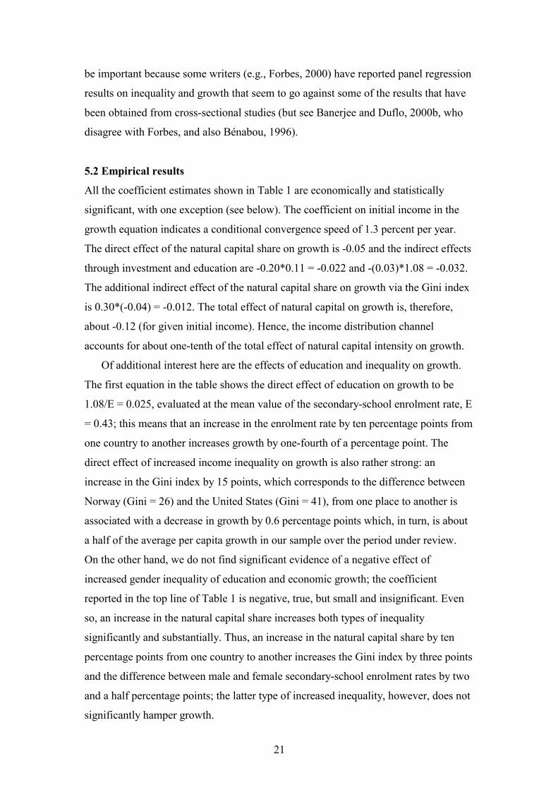
All the coefficient estimates shown in Table 1 are economically and statistically
significant, with one exception (see below). The coefficient on initial income in the
growth equation indicates a conditional convergence speed of 1.3 percent per year.
The direct effect of the natural capital share on growth is -0.05 and the indirect effects
through investment and education are -0.20*0.11 = -0.022 and -(0.03)*1.08 = -0.032.
The additional indirect effect of the natural capital share on growth via the Gini index
is 0.30*(-0.04) = -0.012. The total effect of natural capital on growth is, therefore,
about -0.12 (for given initial income). Hence, the income distribution channel
accounts for about one-tenth of the total effect of natural capital intensity on growth.
Of additional interest here are the effects of education and inequality on growth.
The first equation in the table shows the direct effect of education on growth to be
1.08/E = 0.025, evaluated at the mean value of the secondary-school enrolment rate, E
= 0.43; this means that an increase in the enrolment rate by ten percentage points from
one country to another increases growth by one-fourth of a percentage point. The
direct effect of increased income inequality on growth is also rather strong: an
increase in the Gini index by 15 points, which corresponds to the difference between
Norway (Gini = 26) and the United States (Gini = 41), from one place to another is
associated with a decrease in growth by 0.6 percentage points which, in turn, is about
a half of the average per capita growth in our sample over the period under review.
On the other hand, we do not find significant evidence of a negative effect of
increased gender inequality of education and economic growth; the coefficient
reported in the top line of Table 1 is negative, true, but small and insignificant. Even
so, an increase in the natural capital share increases both types of inequality
significantly and substantially. Thus, an increase in the natural capital share by ten
percentage points from one country to another increases the Gini index by three points
and the difference between male and female secondary-school enrolment rates by two
and a half percentage points; the latter type of increased inequality, however, does not
significantly hamper growth.
21
It is interesting to note that the inclusion of the natural capital share and the
secondary-school enrolment rate in the growth equation does not reverse the sign of
the estimated coefficient of the Gini index. In particular, the relationship between
growth and inequality remains negative, in contrast to the results of Forbes (2000).
However, the size of the income distribution effect is reduced by about a half by the
inclusion of the natural capital and school enrolment variables. This seems to suggest
that in growth equations without natural capital and education, the income distribution
variable picks up a good part of the influence of the omitted variables. Our cross-
sectional results bear out a long-term relationship between inequality and growth
while the pooled estimation of Forbes (2000) reflects short- to medium-term
relationships by her own reckoning. It is also possible that the inclusion of omitted,
country-specific variables other than natural capital and education could reverse the
sign of the coefficient of the Gini index.
Notice, at last, that the data support the notion of a Kuznets curve relating income
inequality and initial income. There is, however, no comparable nonlinear relationship
between gender inequality and initial income. In our data, initial income has no
significant effect on investment across countries.
5.3 Other possibilities
We have experimented with several variations of the model specification in Table 1.
First, we added natural capital per person as a proxy for natural resource
abundance in order to distinguish between natural resource abundance and natural
resource intensity (as in Gylfason and Zoega, 2001b). By intensity, or dependence, we
mean the importance of natural resources to the national economy, while abundance
refers to the supply (per capita) of the natural resources. Some countries – Australia,
Canada and the United States, to name a few – have abundant natural resources but
are not particularly dependent upon them, not any more. Our argument has been that it
is natural resource dependence that matters for inequality and growth. We do not
expect Australia, Canada or the United States to suffer from their abundance of
natural resources, far from it. When we add natural capital per person as an
independent explanatory variable to each equation in Table 1, it turns out that natural
resource abundance encourages economic growth, investment and education and
reduces gender inequality, but has no effect on income inequality. In other respects,
the results remain virtually the same as in Table 1. This means that increased
22

dependence on natural resources hurts growth, as we hypothesized, while increased
abundance helps (for more, see Gylfason and Zoega, 2001b).
Next, we entered the natural capital share and the Gini index of income inequality
multiplicatively rather than additively in our growth equation in order to study the
interaction between the two variables. Now the coefficient of the multiple is -0.0011
(with t = 3.72). This means that the negative effect of natural resource dependence on
growth varies directly with income inequality: the more unequal the distribution of
income, the greater is the adverse effect of natural resource dependence on growth.
Evaluated at the mean value of the Gini index in our sample (42), the effect of the
natural capital share on growth is -0.05 as in Table 1. This new specification also
means that the negative effect of income inequality on growth varies directly with
natural resource dependence: the greater the natural capital share, the greater is the
adverse effect of income inequality on growth. Evaluated at the mean value of the
natural capital share in our sample (12), the effect of income inequality on economic
growth is -0.013, which is smaller than the coefficient of the Gini index in the first
equation in Table 1. When we replace the Gini index of income inequality in the
above experiment with our measure of gender inequality or of land inequality, we
obtain the same results: the greater the natural capital share, the greater is the adverse
effect of increased inequality on growth.
Third, we replaced our gender inequality measure (the arithmetic difference
between male and female secondary-school enrolment rates) by the absolute difference
between male and female enrolment rates. The new measure means that a change from a
situation where more boys than girls go to school to one where more girls than boys
go to school leaves gender inequality unchanged if the numbers are the same. When
we re-estimate our system using this new measure, increased gender inequality
reduces economic growth directly: the coefficient on gender inequality in the first
equation in Table 1 is now -0.05 with t = 2.09. In this case, however, the effect of the
natural capital share on gender inequality becomes small and statistically insignificant
(the coefficient is 0.08 with t = 1.47). In other respects, the regression results (not
shown) are very similar to those reported in Table 1.
Our fourth and last experiment involves Africa and Latin America. When we add
a dummy variable for Africa to each equation in our model, in case Africa might be
different from other regions, as some studies have shown, the dummy coefficient has
the expected sign everywhere, but it is statistically significant only in the equations
23
for education and the Gini index. The annual rate of per capita growth in Africa is
thus three quarters of a percentage point smaller than elsewhere according to our
results (not shown), but the difference is not significant (t = 1.73). The investment rate
is almost two percentage points lower in Africa than elsewhere, but again the
difference is insignificant (t = 1.38). The secondary-school enrolment rate is 15
percentage points lower in Africa than elsewhere (evaluated at the sample mean), and
this difference is significant (t = 3.23). Gender inequality in education is also
significantly greater in Africa than elsewhere, by almost five percentage points (t =
2.15). There is, on the other hand, no significant difference between the Gini index in
Africa and the rest of our sample. All the estimates shown in Table 1 remain
essentially intact in the presence of the African dummy. When we add a dummy
variable for Latin America (with or without Central America) rather than for Africa,
the dummy has no effect on growth, investment or education, but it does matter for
distribution; specifically, the Latin dummy reduces gender inequality by 7.5
percentage points (t = 2.48) and increases the Gini index of income inequality by ten
points (t = 3.20). Again, our estimates in Table 1 remain unchanged. We conclude that
the specification of our model in Table 1 is sufficiently broad to render the inclusion
of regional dummy variables superfluous.
6. Conclusion The inverse empirical relationship between inequality and economic growth across
countries that has emerged from several recent studies has spurred several authors to
suggest various potential theoretical explanations for the relationship. These
explanations have generally been of the following kind: inequality is bad for some
variable X – for example, education – and X is good for growth, so increased
inequality hurts growth by hurting X. We approach this issue from a different angle:
we argue that a country’s dependence on its natural resources influences both
inequality and growth. We show – both theoretically and empirically – how variations
in the share of natural resources in national wealth can help explain the inverse
relationship between inequality and economic growth across countries.
The essence of our story is this: if the distribution of ownership of natural
resources is more unequal than the distribution of other forms of wealth, the
inequality of the distribution of income, education or land is directly related to the
24
share of natural resources in national income. Specifically, we show – in the context
of an endogenous-growth model of the simplest kind – how natural resources can
reduce growth and increase inequality by attracting workers away from higher
technology industries. Our data appear to confirm this prediction: they suggest that
the Gini index of income inequality as well as gender inequality varies directly with
the share of natural capital in national wealth. The data also bear out an inverse
relationship between economic growth and the share of natural capital in national
wealth.
Differences in human capital across countries appear also to help explain the
inverse cross-country correlation between economic growth and inequality. More and
better education – measured by secondary-school enrolment, years of schooling or
public expenditure on education – is associated with less inequality and more rapid
growth in our data. This suggests a clear role for public policy in combating the
potentially adverse effects of excessive dependence on natural resources on income
inequality and growth. In addition, tax policy can be used to combat the adverse effect
of natural resources on inequality and growth. When income or rent from natural
resource extraction is taxed at a higher rate than wage income, this discourages
workers from spending time in the natural resource sector, raises the marginal product
of capital in manufacturing, increases the real rate of interest and thereby also the rate
of growth of output and consumption per capita.
Our regression results suggest that natural capital intensity reduces growth directly
as well as indirectly by reducing equality, secondary-school enrolment rates and
investment rates. This leaves an important role for public policy, which can be used to
encourage growth by enhancing equality, among other things. We conclude that the
trade-off between equality and (dynamic) efficiency is affected by both natural and
human capital, as well as by tax policy.
25
References Aghion, Philippe (1998), with Eve Caroli and Cecilia García-Peñalosa, “Inequality
and Economic Growth,” Part I in Philippe Aghion and Jeffrey G. Williamson,
Growth, Inequality and Globalization: Theory, History and Policy, Cambridge
University Press, Cambridge, England.
Aghion, Philippe, Eve Caroli and Cecilia García-Peñalosa (1999), “Inequality and
Economic Growth: The Perspective of the New Growth Theories,” Journal of
Economic Literature 37, December, 1615-1660.
Alesina, Alberto, and Dani Rodrik (1994), “Distributive Politics and Economic
Growth,” Quarterly Journal of Economics 109, May, 165-190.
Alesina, Alberto, and Roberto Perotti (1996), “Income Distribution, Political
Instability, and Investment,” European Economic Review 40, June, 1203-1228.
Banerjee, Abhijit V., and Esther Duflo (2000a), “Inequality and Growth: What Can the
Data Say?”, Working Paper No. 00-09, Department of Economics, MIT.
Banerjee, Abhijit V., and Esther Duflo (2000b), “A Reassessment of the Relationship
Between Inequality and Growth”, unpublished manuscript, Department of
Economics, MIT.
Barro, Robert J. (2000), “Inequality and Growth in a Panel of Countries,” Journal of
Economic Growth 5, March, 5-32.
Bénabou, Roland (1996), “Inequality and Growth,” NBER Macroeconomics Annual.
Benhabib, Jess, and Aldo Rustichini (1996), “Social Conflict and Growth,” Journal of
Economic Growth 1, March, 124-142.
Bourguignon, François, and C. Morrison (1990), “Income Distribution, Development
and Foreign Trade,” European Economic Review 34, September, 1113-1132.
Bruno, Michael (1984), “Raw Materials, Profits, and the Productivity Slowdown,”
Quarterly Journal of Economics 99, February, 1-28.
Deininger, Klaus, and Pedro Olinto (2000), “Asset Distribution, Inequality, and
Growth,” Working Paper No. 2375, World Bank, Development Research Group.
Deininger, Klaus, and Lyn Squire (1996), “A New Data Set Measuring Income
Inequality,” World Bank Economic Review 10, September, 565-591.
Easterly, William, and Sergio Rebelo (1993), “Fiscal Policy and Growth: An
Empirical Investigation,” Journal of Monetary Economics 32, December, 417-
458.
26
Forbes, Kristin J. (2000), “A Reassessment of the Relationship Between Inequality
and Growth,” American Economic Review 90, September, 869-887.
Galor, Oded, and Joseph Zeira (1993), “Income Distribution and Macroeconomics,”
Review of Economic Studies 60, January, 35-52.
Galor, Oded, and Omer Moav (1999), “From Physical to Human Capital: Inequality
in the Process of Development,” CEPR Discussion Paper No. 2307, December.
García-Peñalosa, Cecilia (1995), “The Paradox of Education or the Good Side of
Inequality,” Oxford Economic Papers 47, No. 2, 265-285.
Gylfason, Thorvaldur (2001), “Natural Resources, Education, and Economic
Development,” European Economic Review 45, May, 847-859.
Gylfason, Thorvaldur, Tryggvi Thor Herbertsson and Gylfi Zoega (2001),
“Ownership and Growth,” World Bank Economic Review 15, October, 431-449.
Gylfason, Thorvaldur, and Gylfi Zoega (2001a), “Obsolescence,” CEPR Discussion
Paper No. 2833, June.
Gylfason, Thorvaldur, and Gylfi Zoega (2001b), “Natural Resources and Economic
Growth: The Role of Investment,” CEPR Discussion Paper No. 2743, March.
Kaldor, Nicholas (1956), “Alternative Theories of Distribution,” Review of Economic
Studies 23, 83-100.
Lahiri, Kajal, and Peter Schmidt (1978), “On the Estimation of Triangular Structural
Systems,” Econometrica 46, 1217-1221.
Paldam, Martin (1997), “Dutch Disease and Rent Seeking: The Greenland Model,”
European Journal of Political Economy 13, August, 591-614.
Perotti, Robert (1996), “Growth, Income Distribution, and Democracy: What the Data
Say,” Journal of Economic Growth 5, June, 149-187.
Persson, Torsten, and Guido Tabellini (1994), “Is Inequality Harmful for Growth?,”
American Economic Review 84, June, 600-621.
Pritchett, Lant (2000), “The Tyranny of Concepts: CUDIE (Cumulated, Depreciated,
Investment Effort) is Not Capital,” Journal of Economic Growth 5, December,
361-384.
Romer, Paul M. (1986), “Increasing Returns and Long-Run Growth,” Journal of
Political Economy 94, October, 1002-1037.
Sachs, Jeffrey D., and Andrew M. Warner (1995, revised 1997, 1999), “Natural
Resource Abundance and Economic Growth,” NBER Working Paper 5398,
Cambridge, Massachusetts.
27
Saint-Paul, Gilles, and Thierry Verdier (1993), “Education, Democracy and Growth,”
Journal of Development Economics 42, 399-407.
Saint-Paul, Gilles, and Thierry Verdier (1996), “Inequality, Redistribution and
Growth: A Challenge to the Conventional Political Economy Approach,”
European Economic Review 40, 719-728.
Scott, Maurice Fitzgerald (1989), A New View of Economic Growth, Clarendon Press,
Oxford.
Sen, Amartya (1999), Development as Freedom, Oxford University Press, Oxford.
Todaro, Michael P. (1997), Economic Development, Longman, London.
World Bank (1997), “Expanding the Measure of Wealth: Indicators of
Environmentally Sustainable Development,” Environmentally Sustainable
Development Studies and Monographs Series No. 17, World Bank, Washington,
D.C.
World Bank (2000), World Development Indicators 2000, World Bank, Washington,
D.C.
28

Table 1. Regression Results
Dependent variable
Initial income
Initial income squared
Natural capital share
Investment rate
Enrolment rate (log)
Gini index
Gender inequality
R2 Countries
Economic growth
-1.26 (6.05)
-0.05 (5.19)
0.11 (3.82)
1.08 (3.88)
-0.04 (2.84)
-0.01 (0.76)
0.68 74
Investment rate
-0.20 (3.98)
0.15 87
Enrolment rate
0.54 (11.31)
-0.03 (6.29)
0.70 87
Gini index 48.88 (3.54)
-3.20 (3.69)
0.30 (2.84)
0.31 74
Gender inequality
0.25 (2.98)
0.09 87
Note: Estimation method: SUR. t-ratios are shown within parentheses. Constant terms are not reported to conserve space.
Figure 1. The Gini Index and the 20/20 Ratio
y = 16.507x + 5.8027R2 = 0.9529
0
10
20
30
40
50
60
70
80
0 1 2 3 4 5
Log of 20/20 ratio (various years)
Gin
i ind
ex (v
ario
us y
ears
)
29
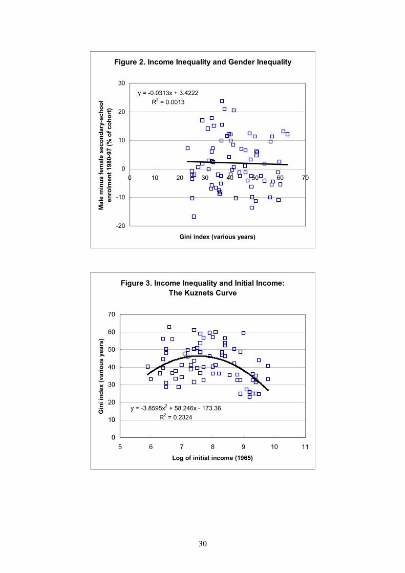
Figure 2. Income Inequality and Gender Inequality
y = -0.0313x + 3.4222R2 = 0.0013
-20
-10
0
10
20
30
0 10 20 30 40 50 60 70
Gini index (various years)
Mal
e m
inus
fem
ale
seco
ndar
y-sc
hool
en
rolm
ent 1
980-
97 (%
of c
ohor
t)
Figure 3. Income Inequality and Initial Income: The Kuznets Curve
y = -3.8595x2 + 58.246x - 173.36R2 = 0.2324
0
10
20
30
40
50
60
70
5 6 7 8 9 10 1Log of initial income (1965)
Gin
i ind
ex (v
ario
us y
ears
)
1
30
Figure 4. Gender Inequality and Initial Income
y = 0.4145x2 - 10.932x + 62.536R2 = 0.2506
-20
-15
-10
-5
0
5
10
15
20
25
30
5 6 7 8 9 10 1
Log of initial income (1965)
Mal
e m
inus
fem
ale
seco
ndar
y-sc
hool
en
rolm
ent 1
980-
97 (%
of c
ohor
t)
1
Figure 5. Distribution of Income and Land
y = 0.9487x + 27.215R2 = 0.3316
0
10
20
30
40
50
60
70
80
90
100
0 10 20 30 40 50 60 70
Gini index for income (various years)
Gin
i ind
ex fo
r lan
d (v
ario
us y
ears
)
31
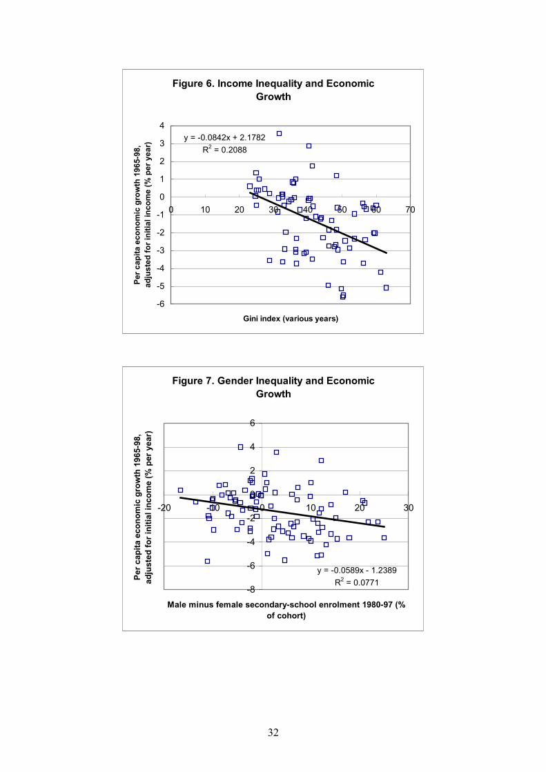
Figure 6. Income Inequality and Economic Growth
y = -0.0842x + 2.1782R2 = 0.2088
-6
-5
-4
-3
-2
-1
0
1
2
3
4
0 10 20 30 40 50 60 70
Gini index (various years)
Per c
apita
eco
nom
ic g
row
th 1
965-
98,
adju
sted
for i
nitia
l inc
ome
(% p
er y
ear)
Figure 7. Gender Inequality and Economic Growth
y = -0.0589x - 1.2389R2 = 0.0771
-8
-6
-4
-2
0
2
4
6
-20 -10 0 10 20 3
Male minus female secondary-school enrolment 1980-97 (% of cohort)
Per c
apita
eco
nom
ic g
row
th 1
965-
98,
adju
sted
for i
nitia
l inc
ome
(% p
er y
ear)
0
32
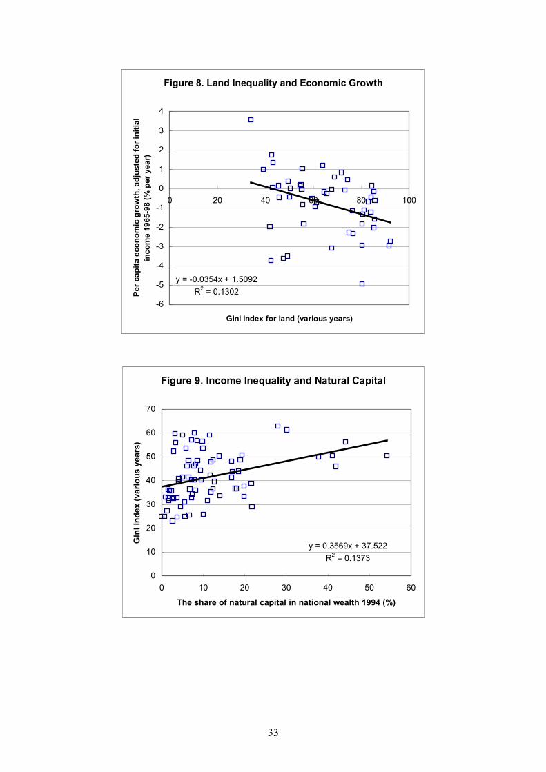
Figure 8. Land Inequality and Economic Growth
y = -0.0354x + 1.5092R2 = 0.1302
-6
-5
-4
-3
-2
-1
0
1
2
3
4
0 20 40 60 80 10
Gini index for land (various years)
Per c
apita
eco
nom
ic g
row
th, a
djus
ted
for i
nitia
l in
com
e 19
65-9
8 (%
per
yea
r)
0
Figure 9. Income Inequality and Natural Capital
y = 0.3569x + 37.522R2 = 0.1373
0
10
20
30
40
50
60
70
0 10 20 30 40 50 60
The share of natural capital in national wealth 1994 (%)
Gin
i ind
ex (v
ario
us y
ears
)
33
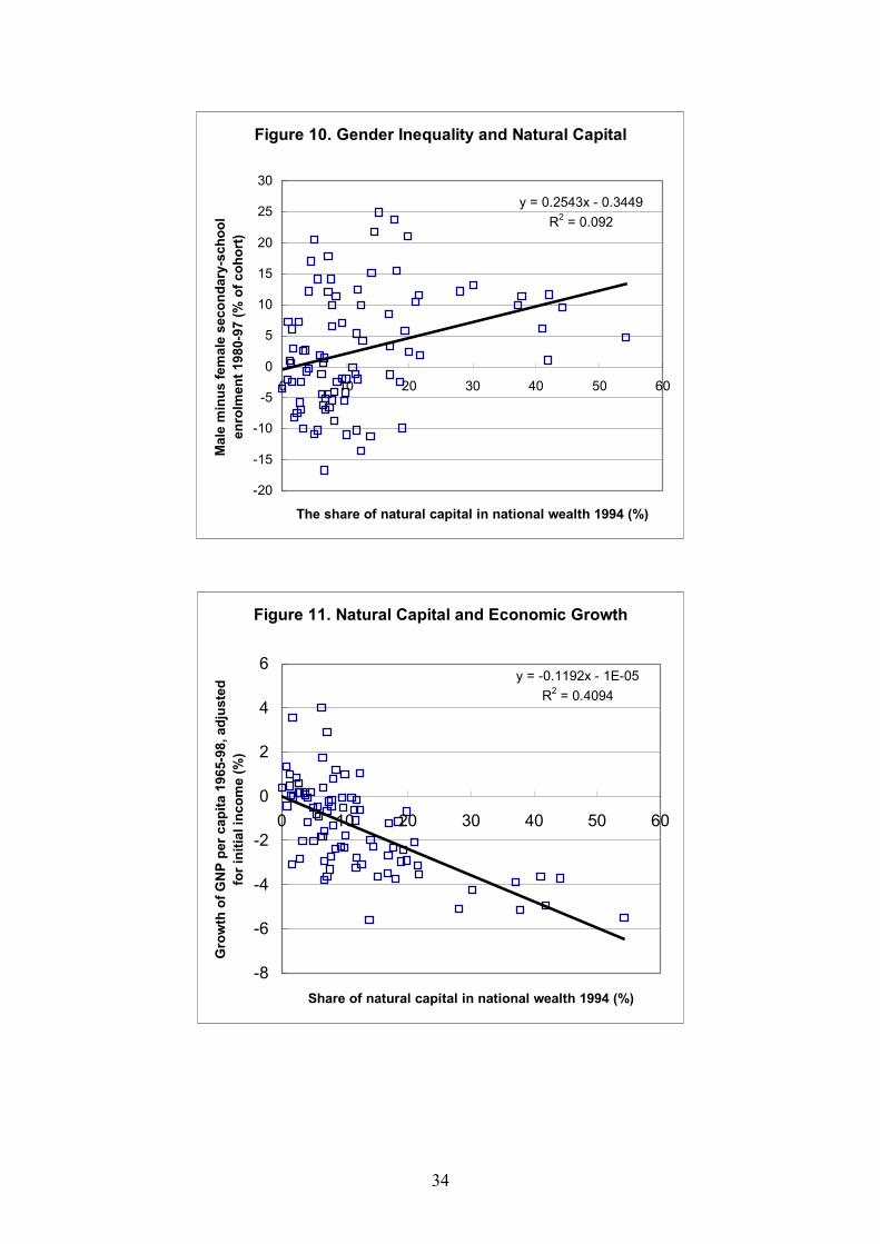
Figure 10. Gender Inequality and Natural Capital
y = 0.2543x - 0.3449R2 = 0.092
-20
-15
-10
-5
0
5
10
15
20
25
30
0 10 20 30 40 50 60
The share of natural capital in national wealth 1994 (%)
Mal
e m
inus
fem
ale
seco
ndar
y-sc
hool
en
rolm
ent 1
980-
97 (%
of c
ohor
t)
Figure 11. Natural Capital and Economic Growth
y = -0.1192x - 1E-05R2 = 0.4094
-8
-6
-4
-2
0
2
4
6
0 10 20 30 40 50 60
Share of natural capital in national wealth 1994 (%)
Gro
wth
of G
NP
per c
apita
196
5-98
, adj
uste
d fo
r ini
tial i
ncom
e (%
)
34

Figure 12. Natural Capital and Expenditure on Education
y = -0.0561x + 4.9044R2 = 0.1247
0
1
2
3
4
5
6
7
8
9
0 10 20 30 40 50 60Share of natural capital in national wealth 1994 (%)
Publ
ic e
xpen
ditu
re o
n ed
ucat
ion
1980
-97
(%of
GN
P)
Figure 13. Expenditure on Education and Income Inequality
y = -2.3106x + 51.494R2 = 0.1318
0
10
20
30
40
50
60
70
0 2 4 6 8
Public expenditure on education 1980-97 (% of GNP)
Gin
i ind
ex (v
ario
us y
ears
)
10
35
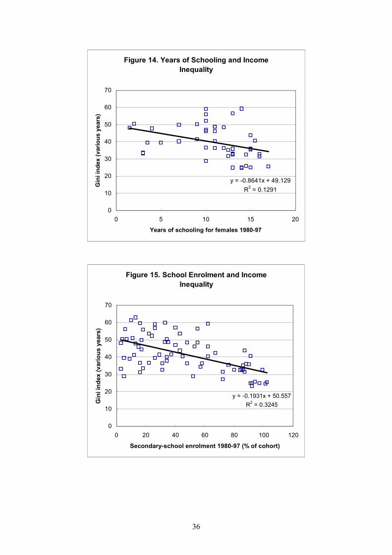
Figure 14. Years of Schooling and Income Inequality
y = -0.8641x + 49.129R2 = 0.1291
0
10
20
30
40
50
60
70
0 5 10 15 20
Years of schooling for females 1980-97
Gin
i ind
ex (v
ario
us y
ears
)
Figure 15. School Enrolment and Income Inequality
y = -0.1931x + 50.557R2 = 0.3245
0
10
20
30
40
50
60
70
0 20 40 60 80 100 120
Secondary-school enrolment 1980-97 (% of cohort)
Gin
i ind
ex (v
ario
us y
ears
)
36


