
Impact of Rooftop Solar on
Distribution Network Planning
Ashish B. Gupta
B.Eng. (Hons.) in Electrical Engineering
ORCID: 0000-0001-9490-0680
Submitted in total fulfilment of the requirements of the degree of
Master of Philosophy
Department of Electrical and Electronic Engineering
Melbourne School of Engineering
THE UNIVERSITY OF MELBOURNE
Victoria 3010, Australia
December 2019

ii
ABSTRACT
Electricity networks have been undergoing significant transformation recently,
especially in terms of embedded generation. There has been a lot of focus on demand
fluctuations from solar and wind farms that are being connected onto high voltage (HV) grids
in energy markets. But the distribution low voltage (LV) grid may prove the most challenging
for the network owners and market operators. This is because rooftop solar, whether installed
in commercial or residential areas, is leading to high demand fluctuations within the last mile.
Customer-installed solar is also causing voltages to rise, but it is the Distribution Network
Operator (DNO) on which the responsibility of voltage regulation falls. There is hence greater
importance for the DNO to have full visibility of the LV feeder voltages at all times,
accurately analysing proposed connections, and meeting the regulators’ and government
expectations of enabling solar penetration.
Voltage monitoring and regulating infrastructure at the LV level, though, is expensive
to implement and hence scarce due to its huge scale. Utilities hence employ empirical or
statistical techniques to calculate voltage drop and voltage rise. Conservative allowances for
demand diversity and unbalance can lead to erroneous results and can form the basis of
considerable utility capital expenditure programs. Utility expenditure in turn usually leads to
an increase in customer bills over time. A small number of utilities in the world have access
to voltage data from smart metering infrastructures, such as in Victoria, Australia, but
ownership of data is becoming an open question. Data availability also presents a different
problem to them, as these meters are leading to an extraordinary amount of near real-time
data, which they are failing to fully embrace. They see smart-technology driven initiatives as
a form of disruption and are slow or unwilling to adapt to the changing nature of the grid.
This dissertation details the use of data analytics for forecasting future voltages on
the network. Standard machine learning techniques are used to create a non-linear regression
model fit to train parameters that reflect the operational status of the feeder. These parameters
reflect load diversity and unbalance as well as generator diversity and unbalance. The trained
model consequently accurately predicts voltages on the feeder with additional connections.
A load-flow simulation of a real-world network is carried out. Training and testing are
performed on data from different halves of the year. Predicted voltages are compared to
simulation results to confirm the high accuracy, even though consumption patterns and solar

iii
irradiation patterns change due to different seasons in the test data. Hence, by leveraging
interval metering data, it is shown how standard machine learning methods can be used to
develop forecasting capabilities.
The methodology developed in this thesis can used as a planning tool to quickly and
accurately evaluate future rate of recurrence of voltage violations; and predict the voltage
headroom available on the LV feeder. This is a significant outcome as predictability of LV
feeder voltages is a concern for the utilities, consumers as well as regulating bodies. The
presented method will enable more loads and PVs onto the network without the need of new
assets such as distribution transformers or LV feeders, that may be left underutilised. It will
also help resolve certain quality of supply issues such as voltage drop complaints; and help
better prioritise and technically analyse constrained areas of the network.
It is clear that high-quality, high-volume data analysis will play a key role in resolving
the needs of the electricity industry. This thesis serves as an interface between network
planning engineers and data scientists who will solve the emerging energy constraints, play a
part in minimising customer energy prices and assist in the transition to decentralised clean
energy sources.

iv
DECLARATION
This is to certify that
i. the thesis comprises only my original work towards the MPhil except where
indicated in the preface;
ii. due acknowledgement has been made in the text to all other material used; and
iii. the thesis is less than 50,000 words in length, exclusive of tables, maps,
bibliographies and appendices.
Ashish Bert Gupta, December 2019

v
ACKNOWLEDGEMENTS
First and foremost, I would like to thank God “Shri Sai Baba” for his blessings and
for helping me achieve my goal of completing this research successfully.
I would like to convey my sincerest and deepest thanks to my Principal Supervisor
Prof. Tansu Alpcan and Co-Supervisor Dr. Anthony B. Morton for their incomparable
support, guidance and encouragement throughout my MPhil. Prof. Tansu Alpcan has been
extremely patient with me, and his knowledge has been invaluable throughout. He has always
sought to instil in me different attributes of a successful researcher, which is very much
appreciated.
I would like to acknowledge the financial support received through an “Australian
Government Research Training Program Scholarship” for covering my tuition fees; and The
University of Melbourne for covering my conference registration fees through a travel
bursary. I would also like to thank Graduate School of Engineering and the Melbourne Energy
Institute for providing presentation opportunities at seminars and symposiums where I was
able to receive constructive feedback from an expert audience.
I am grateful to all the staff and colleagues of the Department of Electrical and
Electronic Engineering and the Graduate Student Association, who gave me advice in
personal and professional matters during my graduate studies; helped me form better writing
and editing practices; and ensured my time at University was a pleasurable experience.
Last, but not least, I am very grateful to all my family members, especially my fiancé
Mrinalini Oswal, for their continuous support and unconditional love which helped me strive
for my goal. I would like to dedicate this thesis to my parents, who have made countless
sacrifices through my schooling and University years.

vi
PREFACE
This work was supported by The University of Melbourne and United Energy. United Energy
provided anonymised interval-reading data from 54 domestic meters on their distribution
network.
Publication included in this thesis – Peer reviewed Conference Paper (1):
A. B. Gupta, T. Alpcan, and A. B. Morton, "Predicting Voltage Variations in Low Voltage
Networks with Prosumers," in 2018 IEEE PES Asia-Pacific Power and Energy Engineering
Conference (APPEEC), pp. 183-188 DOI: 10.1109/APPEEC.2018.8566480, 7-10 October
2018, Kota Kinabalu, Malaysia.
The methodology used in this thesis is incorporated in the above paper [1].
A poster by the same authors on the same methodology was also presented at the Melbourne
Energy Institute Symposium on 12th December 2018 at The University of Melbourne.
All work beyond the above is original, independent work by the author, Ashish Bert Gupta.
Contributions by others to the thesis
“No contributions by others”
Statement of parts of the thesis submitted to qualify for the award of another degree
“None”

vii
Contents
ABSTRACT ........................................................................................................................... ii
DECLARATION .................................................................................................................... iv
ACKNOWLEDGEMENTS ........................................................................................................ v
PREFACE ............................................................................................................................. vi
LIST OF FIGURES .................................................................................................................. x
LIST OF TABLES .................................................................................................................. xii
ABBREVIATIONS AND ACRONYMS ..................................................................................... xiii
CHAPTER 1 – INTRODUCTION ............................................................................................... 1
1.1. Background.................................................................................................................... 1
1.2. Research Motivation ..................................................................................................... 4
1.3. Research Questions ....................................................................................................... 8
1.4. Research Hypothesis and Objectives ............................................................................ 8
1.5. Research Contributions ................................................................................................. 9
1.6. Research Scope and Limitations.................................................................................. 10
1.7. Thesis Outline .............................................................................................................. 11
CHAPTER 2 – LITERATURE REVIEW ..................................................................................... 12
2.1. Solar PV Uptake ........................................................................................................... 12
2.2. Advantages of Solar PV System Integrations .............................................................. 13
2.3. Power Quality Issues with PV System Integrations ..................................................... 16
2.4. LV Feeder Voltage Calculation Methods ..................................................................... 21
2.4.1. Base Line Formulae ............................................................................................. 22
2.4.2. Load Diversity ...................................................................................................... 24
2.4.3. Voltage Unbalance .............................................................................................. 26
2.4.4. Electricity supply industry practice ..................................................................... 29
2.4.5. Feeder voltage estimation – Alternative techniques .......................................... 31
2.5. Research Gap ............................................................................................................... 34
CHAPTER 3 – PROBLEM ANALYSIS ...................................................................................... 36
PART I – BACKGROUND ........................................................................................................... 36
3.1. Victorian Power Networks .......................................................................................... 36
3.2. MV and LV Lines .......................................................................................................... 39
3.2.1. 400V Construction ............................................................................................... 39
3.2.2. Modelling of Distribution Networks .................................................................... 42
3.3. Transformer Construction ........................................................................................... 44

viii
3.4. Voltage Regulation Bandwidth .................................................................................... 48
3.4.1. MV bus ................................................................................................................ 48
3.4.2. MV feeder to distribution transformer ............................................................... 48
3.4.3. Distribution transformer impedance to LV secondary ........................................ 49
3.4.4. Distribution transformer tap offset ..................................................................... 50
3.4.5. LV mains feeder and service wire........................................................................ 50
3.5. Consumption Data from Meters ................................................................................. 51
PART II – MODEL CONSTRUCTION .......................................................................................... 52
3.6. Software Tools ............................................................................................................. 52
3.7. 22-Bus Unbalanced Distribution Network .................................................................. 53
3.8. Conductor Impedance Characteristics ........................................................................ 57
3.9. Model Inputs from Meter Data ................................................................................... 58
3.10. Micro Embedded Generator Connection ................................................................ 58
3.11. Data Visualisation .................................................................................................... 59
CHAPTER 4 – PARAMETRIC MODELLING FOR MACHINE LEARNING ...................................... 63
4.1. Background.................................................................................................................. 64
4.2. Non-Linear Regression Fit – Implementation ............................................................. 66
4.3. Testing Data and Validating Predictions ..................................................................... 68
4.4. Decision Tree ............................................................................................................... 70
4.5. Validation Calculations ................................................................................................ 72
CHAPTER 5 – RESULTS AND DISCUSSION............................................................................. 74
5.1. Case Network 1 ........................................................................................................... 74
5.1.1. Learning and Testing on Training Set A – LM Validation ..................................... 74
5.1.2. Learning and Testing on Training Set A – CART Validation ................................. 76
5.1.3. Learning with Training Set A and Testing on Test Set A using LM ...................... 77
5.1.4. Learning with Training Set A and Testing on Test Set A using CART ................... 80
5.1.5. Learning with Training Set B and Testing on Test Set B using LM ....................... 81
5.1.6. Learning with Training Set B and Testing on Test Set B using CART ................... 84
5.2. Case Network 2 – High PV Penetration ....................................................................... 86
5.2.1. Learning with Training Set C and Testing on Test Set C using LM ....................... 87
5.2.2. Learning with Training Set C and Testing on Test Set C using CART ................... 88
5.2.3. Learning with Training Set D and Testing on Test Set D using LM ...................... 89
5.2.4. Learning with Training Set D and Testing on Test Set D using CART ................... 92
5.3. Summary and Discussion............................................................................................. 94
CHAPTER 6 – CONCLUSIONS ............................................................................................... 96
6.1. Summary of Thesis ...................................................................................................... 96

ix
6.2. Summary of Contributions .......................................................................................... 99
6.3. Future Works ............................................................................................................. 101
REFERENCES: ................................................................................................................... 103
APPENDIX A: CASE NETWORK 1 CONFIGURATION DATA ................................................... 112
APPENDIX B: SAMPLE INTERVAL METERING DATA FOR ONE HOUSEHOLD ......................... 113
APPENDIX C: OPENDSS AND MATLAB CODE ..................................................................... 115

x
LIST OF FIGURES
Figure 1 – Levelised cost of a 7 kW PV unit vs. retail electricity price (data: [6]) ................ 2
Figure 2 – Number of installations for rooftop PV in Australia (data: [7]) ........................... 2
Figure 3 – Zone Substation load profile year-on-year duck curve [8].................................... 3
Figure 4 – Segmentation of PV installation 2011-2017 [14] ................................................... 12
Figure 5 – Average system size of rooftop PV in Australia (data: [7]) ................................. 13
Figure 6 – Residential energy storage installations in Australia 2015-2017 (data: [19]) .... 14
Figure 7 – Typical voltage sag (dip) and swell waveform representation [36] .................... 19
Figure 8 – Impact on Australian networks with varying PV Penetration Rates [38] ......... 21
Figure 9 – Single-line representation of a single residential load in a 2-bus load flow ....... 22
Figure 10 – Typical coincidence factor curve for residential consumers in USA [62] ........ 26
Figure 11 – Balanced three-phase LV circuit ......................................................................... 27
Figure 12 – Balanced three-phase voltage/ current waveforms ............................................ 27
Figure 13 – Unbalanced three-phase LV circuit ..................................................................... 27
Figure 14 – Typical unbalanced three-phase voltage/ current waveforms .......................... 27
Figure 15 – Operating areas of the Victorian electricity distributors [87] .......................... 36
Figure 16 – Comparison of North American and European Systems [88] .......................... 38
Figure 17 – Typical Pole top construction in Australia [91] .................................................. 40
Figure 18 – LV cross-arm phase separation details [91] ....................................................... 40
Figure 19 – Heat-map of number of overvoltages within United Energy’s area ................. 43
Figure 20 – Heat-map of duration of overvoltages within United Energy’s area................ 43
Figure 21 – Typical pole-mount transformer supplying end user customers ...................... 45
Figure 22 – Picture of a pole-mount transformer in suburban Melbourne ......................... 46
Figure 23 – Tap setting and nameplate of a 200 kVA pole mounted transformer .............. 46
Figure 24 – Average voltage lowers after tap down operation [96] ...................................... 47
Figure 25 – MV feeder line-to-neutral voltage profile upstream of Case Network 1 .......... 49
Figure 26 – MV feeder current profile upstream of Case Network 1 ................................... 49
Figure 27 – Picture of an AMI meter installed in a suburban house in Melbourne ........... 51
Figure 28 – Example of an 8 bus LV network [100] ............................................................... 53
Figure 29 – Spatial representation of multiple branched radial LV network diagram ...... 54
Figure 30 – GIS snapshot of Case Network 1 ......................................................................... 55
Figure 31 – Average P and Q for all households .................................................................... 56
Figure 32 – Cumulative P and Q load downstream of substation ........................................ 56
Figure 33 – Cumulative P and Q load in the east circuit ....................................................... 57
Figure 34 – Cumulative P and Q load in the west circuit ...................................................... 57
Figure 35 – Average annual PV generation profile ................................................................ 58
Figure 36 – Voltage profile at Bus 22 ...................................................................................... 59
Figure 37 – Demand profile at the Substation ........................................................................ 60
Figure 38 – Load and voltage profiles for a high demand day .............................................. 60
Figure 39 – Voltage at load end of each line of Case Network 1 ........................................... 61
Figure 40 – 3-phase average voltage at load end of each line of Case Network 1................ 62
Figure 41 – Unsupervised Learning and Supervised Learning [102] ................................... 65
Figure 42 – Workflow for machine learning and validating predictions (grey box) ........... 69

xi
Figure 43 – Workflow for machine learning and validating predictions (black box) ......... 71
Figure 44 – Learning and Testing on Training Set A using LM ........................................... 75
Figure 45 – Learning and Testing on Training Set A using LM replotted .......................... 75
Figure 46 – Learning and Testing on Training Set A using CART ...................................... 76
Figure 47 – Learning and Testing on Training Set A using CART replotted ..................... 77
Figure 48 – Expected and predicted results of Set A using LM ............................................ 78
Figure 49 – Learning with Training Set A and Testing on Test Set A using LM ................ 78
Figure 50 – Comparing the voltage drop calculation using new parameters ...................... 79
Figure 51 – Expected and predicted results of Set A using CART ....................................... 80
Figure 52 – Learning with Training Set A and Testing on Test Set A using CART ........... 81
Figure 53 – Expected and predicted results of Set B using LM ............................................ 82
Figure 54 – Learning with Training Set B and Testing on Test Set B using LM ................ 82
Figure 55 – Expected and predicted results of Set B using CART ....................................... 85
Figure 56 – Learning with Training Set B and Testing on Test Set B using CART ........... 85
Figure 57 – Expected and predicted results of Set C using LM ............................................ 87
Figure 58 – Learning with Training Set C and Testing on Test Set C using LM ................ 88
Figure 59 – Expected and predicted results of Set C using CART ....................................... 89
Figure 60 – Learning with Training Set C and Testing on Test Set C using CART ........... 89
Figure 61 – Expected and predicted results of Set D using LM ............................................ 90
Figure 62 – Learning with Training Set D and Testing on Test Set D using LM ................ 90
Figure 63 – Expected and predicted results of Set D using CART ....................................... 93
Figure 64 – Learning with Training Set D and Testing on Test Set D using CART ........... 94
Figure 65 – Line-to-Neutral voltage for the three circuits at the last time instance.......... 116
Figure 66 – Demand profile at the substation ....................................................................... 117

xii
LIST OF TABLES
Table 1 – System Voltage Requirements under Australian Standards [32] ................................ 17
Table 2 – Voltage and Frequency Inverter Set Points in Australia [16] ...................................... 19
Table 3 – Voltage Harmonic Distortion Limits in Victoria ........................................................... 20
Table 4 – Summary of All Variables Used .................................................................................... 23
Table 5 – Transformer impedances typically used in Australia at 75°C [90] ............................... 47
Table 6 – Typical Voltage Bandwidth Contributions in LV Feeder .............................................. 50
Table 7 – Characteristics of the chosen LV network ................................................................... 55
Table 8 – Comparison of RMSE (V) – Training and Testing on the Same Data Set ..................... 77
Table 9 – Parameter Comparison For Set A ................................................................................ 79
Table 10 – Comparison of RMSE (V) ............................................................................................ 79
Table 11 – Parameter Comparison For Set B .............................................................................. 83
Table 12 – Case Network 1 – Parameter Comparison For West Circuit – To Bus 9 .................... 83
Table 13 – Case Network 1 – Parameter Comparison For East Circuit – To Bus 16 .................... 84
Table 14 – Case Network 1 – Parameter Comparison For East Circuit – To Bus 22 .................... 84
Table 15 – Comparison of RMSE Betweeen Black Box and Grey Box Methods (V) .................... 86
Table 16 – Parameter Comparison For Set C .............................................................................. 88
Table 17 – Parameter Comparison For Set D .............................................................................. 91
Table 18 – Case Network 2 – Parameter Comparison For West Circuit – To Bus 9 .................... 91
Table 19 – Case Network 2 – Parameter Comparison For East Circuit – To Bus 16 .................... 92
Table 20 – Case Network 2 – Parameter Comparison For East Circuit – To Bus 22 .................... 92
Table 21 – Comparison of RMSE Betweeen Black Box and Grey Box Methods (V) .................... 94
Table 22 – Line Lengths Modelled In OpenDSS ......................................................................... 112
Table 23 – Metering Data For A Resident In Case Network 1 For One Day .............................. 113

xiii
ABBREVIATIONS AND ACRONYMS
AAC All Aluminium Conductor
ADLDD After Diversity Lowest Daytime Demand
ADMD After Diversity Maximum Demand
AER Australian Energy Regulator
ALARP As Low As Reasonably Practicable
AMI Advanced Metering Infrastructure
API Application Programming Interface
AS Australian Standard
AS/NZS Australian/New Zealand Standard
CF Coincidence Factor
CART Classification and Regression Trees
DF Diversity Factor
DEBUT Demand Estimation Based on Units of Time
DG Distributed Generation
DNO Distribution Network Operator
EHV Extra High Voltage
EPRI Electric Power Research Institute
EV Electric Vehicle
FCAS Frequency Control Ancillary Services
GIS Geographic Information System
HV High Voltage
IEEE Institute of Electrical and Electronics Engineering

xiv
LCF Load Correction Factor
LCOE Levelised Cost of Energy
LM Levenberg-Marquardt
LV Low Voltage
MD Maximum Demand
MSE Mean Squared Error
MV Medium Voltage
NMI National Meter Identifier
OLTC On-Load Tap Changer
PF Power Factor
POE Probability of Exceedance
PQ Power Quality
PV Photovoltaic
SCADA Supervisory Control And Data Acquisition
SCF Solar Correction Factor
SWER Single Wire Earth Return
UF Unbalance Factor
VD Volt-Drop

1
CHAPTER 1 – INTRODUCTION
1.1. Background
As the world continues to electrify towards universal energy access, the electricity
consumption continues to grow strongly. There is expected to be an increase in middle class,
their expendable income and their needs for space cooling equipment, electric vehicles (EV)
and digitalisation. Recently there has been an increasingly conscious effort to move away
from coal and gas-powered power plants to meet these energy needs, as formalised by the
2015 Paris Agreement on Climate Change [2]. Since then, many nations have introduced
personal ambitions and climate policies to move towards renewable sources of electricity
generation. The proportion of fuels being used for generation is hence moving towards more
non-fossil-based resources like wind, nuclear, hydro and solar power plants including rooftop
Photovoltaics (PV). Trends [3] say renewable energy generation from wind and solar will
account for half of the world’s power by 2050. Coal and gas will play less and less vital roles
in the energy generation mix owing to those climate policies and better air quality
management. An example of this is China’s drive to “make the skies blue again” [3].
Solar PV is also on track to be the cheapest source of electricity in many countries.
The Levelised Cost of Energy (LCOE) is the cost of energy per kWh produced, and describes
the cost of the power produced by solar over a period of time. China has the levelised costs
of new solar PV set to fall below those of new coal-fired power plants by the late 2020s [4].
Together with the drive to clean energy and the high prices of coal and gas-powered
plants, renewable energy sources are growing rapidly. Distributed solar generation (rooftop
PV) uptake especially, is being driven by increased consumer awareness and Government
2
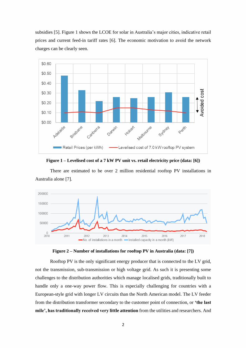
subsidies [5]. Figure 1 shows the LCOE for solar in Australia’s major cities, indicative retail
prices and current feed-in tariff rates [6]. The economic motivation to avoid the network
charges can be clearly seen.
Figure 1 – Levelised cost of a 7 kW PV unit vs. retail electricity price (data: [6])
There are estimated to be over 2 million residential rooftop PV installations in
Australia alone [7].
Figure 2 – Number of installations for rooftop PV in Australia (data: [7])
Rooftop PV is the only significant energy producer that is connected to the LV grid,
not the transmission, sub-transmission or high voltage grid. As such it is presenting some
challenges to the distribution authorities which manage localised grids, traditionally built to
handle only a one-way power flow. This is especially challenging for countries with a
European-style grid with longer LV circuits than the North American model. The LV feeder
from the distribution transformer secondary to the customer point of connection, or ‘the last
mile’, has traditionally received very little attention from the utilities and researchers. And

3
it is becoming increasingly hard for engineers to resolve technical issues borne by PV
penetration, such as increasing variability in system demand, low daytime demand and
increased ramping at morning and evening electricity system peaks.
As rooftop PV penetration grows, a ‘duck curve’ is noticed by DNOs. As seen in
Figure 3 for a substation in Australia, it has the following characteristics during a week day
(Monday to Friday):
• The lowest demand on the feeder consistently drops year-on-year. This is usually
around noon when demand is low and solar back-feed is high; whereas in the past,
the lowest demand used to be around 3 am when there was no back-feed but also very
low demand. Of late, the lowest demand on the feeder can be zero or negative (reverse
power flow due to peak solar back-feed) in areas of low heating requirements.
• The peak demand on the feeder does not reduce during the evening loads. This
demand, in fact, increases with population growth.
• Total energy consumption (kWh) or area under curve reduces.
• The growing gap between highest and lowest demand creates voltage regulation
issues on MV (Medium Voltage) and LV feeders.
Figure 3 – Zone Substation load profile year-on-year duck curve [8]
There also remain other technical issues such as system capacity to accommodate
millions of distributed energy resources, power quality, harmonic distortion, future capital
and operating expenditure (stranded assets), After Diversity Maximum Demand (ADMD)
assessment, protection in low fault-level locations, and data management processes with
regard to device control and new connections. ADMD is the coincident maximum demand,

4
averaged over a large number of customers. ADMD provides a representation of the
maximum demand contribution per customer during peak load, and serves as a theoretical
minimum bound when used for voltage drop calculations. Since ADMD does not take into
account the diversity of the customers’ load at the LV level, using it as the load for all
consumers is not a realistic case. All voltage drop calculations hence take into account an
allowance, in some form, for the loss of diversity from the average current. Additionally,
allowance should also be made for higher voltage drop in practice caused by the current in
the neutral conductor, compared to that caused by balanced loading across the three phases.
This research will aim to understand the implications of the integration of residential solar
power on the network voltages i.e. voltage rise and the planning implications on the existing
steady state voltage management issues such as voltage drop and phase imbalance. Reliable
modelling and simulation of real LV networks in suburban Victoria, Australia will be carried
out with real network configurations and data. We will be looking to predict voltage
variations when new prosumers are added onto the network.
1.2. Research Motivation
In Australia, rooftop PV systems have achieved moderate penetration in the grid and
the number of installations is rising. There are already issues arising within the grid that was
only designed for a one-way power flow. These issues include:
• Localised voltage rises when excess PV generation is exported into the grid;
• Excessive current flowing in neutral conductors caused by unbalance between load
and generation in the three supply phases, creating safety hazards;
• Load unbalance in the three-supply phases causes overloading of assets, impacting
supply reliability and asset life; and
• Tripping of solar inverters on over-voltage protection, so PV customers are not
getting return on their PV investment.
From an LV planning engineer’s perspective, system stability and robustness of
network voltages in newly ‘active’ feeders are of primary importance. With a view on
reducing the amount of new infrastructure required, the predictability of LV feeder voltages
is emerging to be a significant challenge [9].

5
When responding to new power supply applications, distribution network engineers
are required to calculate voltage drop values downstream of existing distribution transformers
at the street level. In case the expected voltage drop from the transformer secondary to the
point of supply is too large, even if supply capacity from existing infrastructure is available,
augmentation works such as feeder upgrades or new distribution transformers are required.
Other utility works such as reducing the number of transformer overloads, fuse overloads,
number of customers connected to a single LV feeder or resolving certain quality of supply
complaints; all require voltage drop calculations done in order to obtain an economical and
technically appropriate solution.
Excessive voltage drop leads to a surge in power quality issues and complaints from
residents. Large voltage drop is primarily due to long distances from the distribution
transformer and/ or voltage imbalance across the LV phases. Over the past few years though,
there has also been a sharp increase in voltage rise complaints from residents in rural areas
with high penetration of large PV panel installations or in urban high-density areas with large
clusters of PV panel installations. Distribution Network Operators (DNOs) employ a few
different strategies to remedy voltage non-compliance without rebuilding the distribution
substations, as this is a considerable expense and not in line with the ALARP ("as low as
reasonably practicable”) approach that many businesses and utilities alike employ. Some of
the other strategies include:
• Reducing the sending end voltage by changing the tap or the turns ratio on the
distribution transformer. This is not always possible though, as the DNO could create
an under-voltage condition during peak load period or could not have any lower tap
positions available;
• Upgrading radial single-phase feeders to three-phase;
• Installing thicker LV conductor or cable to avoid congestion and reduce impedance;
• Swapping more customers onto the phase with excess PV generation, but this could
create overload condition during peak load period when there is little PV generation;
• Limiting solar exports (not community friendly);
• Installing new LV circuits; or
• Re-arranging network switches.
Some of the strategies can also work against one another. For example, installing a
new distribution transformer to off-load peak demand on an existing transformer in the
neighbourhood, could exacerbate existing daytime voltage rise complaints (due to large PVs)

6
in the area. This example presents a daunting prospect as the upgrading of distribution
network is an expensive exercise, and in this example has led to a worse-off customer
experience. This utility then becomes understandably reluctant to network augmentation in
the future. Knowledge of existing and future LV feeder voltages, during times of both peak
and low demand, is hence a key decision driver for the aforementioned strategies.
Load flow analysis of the LV network should hence be done when assessing new
supply or embedded generation calculations. Utilities can then comprehensively examine
impedance levels in feeders, voltage regulation and stability throughout their networks. This
is a manual process and the cost of these studies as suggested here is prohibitive for the large
volume of applications a utility receives. These studies are normally only done for
commercial and industrial rooftop PV installations (say larger than 30 kW three-phase or
another size arbitrarily chosen by DNOs as the demarcation between micro embedded
generators and embedded generators). Even so, these studies are usually done for a single
point in time (worst case), not for an entire year’s worth of data as is ideal.
For residential areas, DNOs have instead relied on various stochastic means to make
these voltage assessments, as discussed in Section 2.4. In managing traditional distribution
networks with unidirectional flow, there was limited need for monitoring of the LV feeder as
it was typically set up so that the range of anticipated voltages did not exceed the allowable
voltage limits. This has served industry well due to ease-of-use. However, increased
distributed energy resources have created active (instead of the erstwhile passive) distribution
networks, and these methods require further evaluation and revision. Utilities are increasingly
wary of allowing increased PV penetration as that may lead to dramatic excursions outside
the allowed voltage limits with subsequent rooftop solar inverter tripping. On the other hand,
declining PV connections, or solar export limits, or large network augmentations to enable
solar connections are also not the optimum solutions. Hence significant enhancement of
voltage calculation techniques is required to best analyse the connection of distributed
energy resources within the safe technical range of the network’s capacity, and to allow for
optimising the performance of the integrated network with its connected devices.
A small number of advanced nations do have access to voltage data from smart
metering infrastructure. This is leading to an extraordinary amount of near-real time data.
Utilities though are failing to gather this data and to use the information thus gathered for
identifying feeders that might be compromised in the future. Utilities need to adapt to new
technologies and proactively address voltage constraints due to both large loads and

7
embedded generation, in an attempt to position themselves well for the future. The best way
to manage voltage issues and integrate increasing levels of solar into electricity distribution
networks, while reducing the need for large-scale investment in the system, should be to
develop a smarter and more flexible grid that is optimised for local voltage conditions. This
is the most optimal solution not just according to utilities and the regulators, but also
according to consumer groups. Community attitudes towards potential solar infrastructure
investment show [10] that prosumers are demanding network improvements that can handle
greater volumes of solar and avoid more expensive investments that show up in electricity
bills.
One of the main motivations of this research is to demonstrate to electricity utilities
that machine learning is an appropriate tool to forecast load voltage and enable higher
share of renewable embedded generation in the system. Exploiting the insights contained
within large data sets has become a focus for a multiplicity of enterprises. Utilities are in a
position to collect a wealth of data on power usage, courtesy of interval metering, including
smart meters. Data analytics technology can be deployed by electricity companies to exploit
usage data in order to forecast LV feeder voltages for a range of conditions.
The other main motivation is to come up with a model that utilities can retrofit into
existing voltage estimation tools. This will lead to minimal re-engineering of the existing
planning methods and will also be well-understood and adopted by industry professionals
at large. The end-result is a method that helps voltage regulations calculations quickly and
accurately i.e. grey box model. Grey box model, as used here, is a model where the engineer
has some knowledge over the internal workings of the methodology and doesn’t face a steep
learning curve. The methodology is said to be somewhat translucent to the end-user. This has
advantages when compared to a black box or closed box model (where internal behaviour is
not known or understood by the user); and the white box or clear box model (where the user
has full knowledge of the internal workings of the application but faces a time-consuming
and exhaustive process). Performing machine learning which presents no trained parameters
to the users, just the end result, can be seen as a black box in our context. Performing load-
flow simulations is seen as a white box.
The end result is a planning framework or tool that then help the utility avoid costly
network upgrades or over-investment. Large utility capital expenditure is often seen as ‘gold-
plating’ of the network in the eyes of consumer groups and regulators, and avoiding these is
hence in line with the customer’s requirements of low power bills. Furthermore, there is a

8
large degree of ‘future-proofing’ prospects available through this method since it avoids the
need to revisit sites every few years to fix issues that could have been foreseen and prevented
in the first instance.
1.3. Research Questions
In the previous section we have identified the challenges being faced by engineers
trying to estimate the LV feeder voltages, with or without penetration of PV. In order to
clarify the aim and purpose of this research and find the appropriate approach, the following
research questions were raised:
a) What impact does PV have on distribution networks? Is this the same all around the
world? This has been discussed in Section 2.3. Note that in discussing distribution
networks, we have taken a generalist approach and not discussed all the different
subtle variations that exist the world over.
b) What are the key components, topologies and parameters of LV distribution networks
in Australia? This has been discussed at length in Chapter 3.
c) Given increasing PV penetration, what are all the different methods employed to
obtain LV feeder voltages, besides load flow modelling and simulations? This has
been discussed in Section 2.4.
d) Has there been any significant enhancement of voltage and headroom calculation
methods in the age of interval metering data? Has there been an attempt to forecast
feeder voltages? This has been explored in Chapter 2.
e) Is machine learning an appropriate tool for predicting voltage data with new
prosumers? Will this be seen as a black box model and hence not find ready adoption
in industry? This has been discussed in Chapter 4.
1.4. Research Hypothesis and Objectives
The hypothesis of this research can be summarised as follows: “There exists risk and
inaccuracies when not estimating feeder voltages from load flow simulations or deterministic
bottom-up modelling respectively. But a standard machine learning technique can be used to
train a set of simple parameters representing the load and PV diversity and imbalance. This
can act as a readily applicable extension to current voltage calculation approaches and

9
traditionally developed methodologies, for the purposes of improving the accuracy of LV
residential network planning and foreseeing constrained parts of the network.”
The main aims of this research hence are as follows:
• Create a new methodology for feeder voltage estimation with new prosumers.
Voltage assessments that are done on a large number of networks should not be too
approximate or conversely too data-intensive. There is a need for a balanced
approach, where the voltages are calculated not in a purely stochastic manner, but
also not purely deterministic so as to require detailed modelling and simulation for
every individual network.
• Create a methodology that is easily adaptable to industry practices. Voltage drop
estimation in the current Australian electricity industry relies on parameters of load
diversity and unbalance. Looking to create a simple method that also generates these
parameters can greatly help in comparison, understanding and interpretation amongst
industry professionals.
1.5. Research Contributions
In this section, the research contributions are detailed:
• The first contribution of this work is the literature survey done on all the differing
methods out there in industry and academia of calculating voltage drop and rise in
LV feeders. This should prove useful to other network planners and researchers alike.
Insights gained into the Australian and New Zealand markets was that interval
metering data was not being used to forecast voltage excursions or foresee
constrained LV feeders.
• Secondly, this thesis presents a modern way of estimating feeder voltages, avoiding
a worst-case scenario deterministic approach, or a conservative probabilistic one. A
data-science approach is taken to determine load and generation correction factors
that can be applied to ADMD when performing feeder voltage calculations. The
proposed method calculates accurate voltage rise in the LV feeder in-case of bi-
directional power flow as well. Parameters of a non-linear regression model fit are
trained, a grey box model, useful for comparison and retrofitting to the status quo.

10
• Machine learning is also used for creating a black box model, useful for finding
voltage headroom at each bus. The results from the grey box model and the black box
model are then compared.
• This work demonstrates an application where machine learning and data analytics can
be used in resolving today’s and future problems associated with the LV grid.
Application of this methodology will enhance a distributor’s knowledge of the
operational conditions of its LV feeders. This will facilitate more informed technical
assessments of prosumers being connected onto the grid, and therefore enable better
utilisation of assets.
1.6. Research Scope and Limitations
In this research, power consumption data from half-hour interval-metering i.e. billing
information has been used. This may present a limitation since retailers or utilities may not
be willing to share private consumer data with third-party electrical contractors or consultants
looking to do voltage assessments for their clients.
If wanting to use smart meter data to carry out this methodology, a utility might face
potential complications if the metering process is taken away from them becomes contestable.
The consumer could then choose from an open competitive market, the installer of the smart
meter and the subsequent ownership of data hence becomes an open question. This is slated
to happen in 2021 in Victoria [11] for example. We have not used smart meter data for our
research.
Where household load data is available, data integrity is paramount. In the data set
used in this research, data obtained for all residences unfortunately contain null values for
reactive power for 6 days in the year. Hence, a consistent voltage drop for those 6 days is not
achieved when the simulation is completed. This is noticeable for all loads on the network.
However, this does not have an overbearing impact on results or methodology proposed.
PV data on the case network was not made available by the utility. And household
PV data from a different network within the same city is used instead. The assumption is
made that PV data used is representative of the PV data of the pertinent case network, were
they available.

11
The work covered in this research covers branched or radial 3-phase, 4-wire LV
systems only. Looped networks or other LV networks such as 2-phase 3-wire or single phase
will not be covered in this work.
1.7. Thesis Outline
The next chapter investigates the research questions posed in Section 1.3 through an
extensive literature review. An example network model is presented and discussed in Section
3.7. Chapter 3 also details the methodology used. This includes extending the state-of-the-art
to allow for voltage rise calculations. In Chapter 4, we propose machine learning models to
calculate parameters for coincidence and unbalance of both load and generation to predict
voltage regulation along LV feeders with new connections. We fit a predefined multivariate
function to a set of points. Chapter 5 details the results and findings. Chapter 6 concludes the
work done for this research and highlights the main findings regarding the potential for, and
limitations of proposed voltage prediction methodologies of distribution feeders with rooftop
PVs. The possible future directions of further research are also presented in this chapter.
Appendices contain other relevant information concerning the dissertation, useful in further
understanding.
One publication has been borne out of this research work. The methodology used
herein is presented in our conference paper: "Predicting Voltage Variations in Low Voltage
Networks with Prosumers" [1].

12
CHAPTER 2 – LITERATURE REVIEW
2.1. Solar PV Uptake
The world has an abundance of sunlight and wind to fuel solar and wind power plants;
and enough geographical space to house such industries on a massive scale. Solar is the fastest
growing power generation source. More solar PV capacities were installed globally than any
other power generation technology. In 2017 alone, almost as much solar was installed in one
year, as total worldwide capacity till 2012 [12]. In particular, distributed generation (rooftop
PV) systems, had an estimated grid connection of 37 GW in 2017, nearly twice that of 20
GW in 2016. This was the first real growth in years, primarily due to policies implemented
in China. The Chinese market continues to grow excessively also on the back of production
capacity expansion. According to recent announcement by the Chinese government, PV
systems will have more room for growth [13].
Figure 4 – Segmentation of PV installation 2011-2017 [14]

13
In Australia, the average PV system size is now over 6 kW as seen in Figure 5,
although some of that is a reflection of larger commercial rooftop systems being installed
with residential rooftop systems sitting around 5 kW. The Australian market remains bullish
for rooftop PV with more than one if five homes having solar PV with the highest per capita
penetration in in the world. The first half of 2018 saw record new PV connections seen since
the early days of premium feed-in-tariffs in 2011-12. PV rooftop systems can compete on
retail price with grid power at most places in the world; yet only few countries, like Australia,
have been truly adopting the solar solution.
Figure 5 – Average system size of rooftop PV in Australia (data: [7])
2.2. Advantages of Solar PV System Integrations
There are certainly some positive aspects of this growing rooftop PV market. Small
solar systems can be the backbone of a digitalized, decarbonized, distributed and
democratized energy system, which empowers consumers and territories (e.g. households,
hospitals, public buildings, hotels, etc.) with cleaner, cheaper and local electricity [12]. They
can bring about a reduction in power bills and social benefits such as job creation. Other
benefits can include: -
Sustainable Energy: In today’s rapidly changing energy market, it is critical for
DNO’s to understand and respond to their customers’ needs. Any draft plans for the future
should deliver in accordance with the needs of the community. There exists a very large
demand of generating green power at the household, business or precinct level alike. Rooftop
PV furthers the aspirations of the community to consume energy produced from only
sustainable resources. DNO’s that allow for the integration of customer installed PV systems,
will empower and educate consumers and allow themselves to be better positioned for a future
with lower CO2 emissions and cleaner air.

14
Resilience and System Reliability: Since there is no in-built contingency at the
residential or street level, a fault or fuse event can force many customers off supply till the
time the issue can be located and supply restored. In theory, back-feed from PV can be used
as back-up supply during black-outs or when there has been an upstream fuse event. This is
especially useful in emergencies such as disaster events or for customers on life-support
apparatus.
Others: PVs have been shown to extend the life of a transformer by extending the
cyclic rating of transformers. PVs reduce the daytime peak demand, so they can hence reduce
transformer loss of life [15]. PV inverters with VAR control improve voltage regulation
(countering the issues that PVs themselves create) if there is sufficient upstream reactance.
Since ∆𝑉 ≈ ∆𝑃 x 𝑅 + ∆𝑄 x 𝑋, VAR absorption by inverters can mitigate voltage rise. Indeed,
this is one of the three ways the Australian standards for PV grid-connected inverters [16]
specify how inverters should respond to high or low grid voltages (and high or low grid
frequency). PV inverters can also act as active filters to reduce system harmonics and negative
sequence unbalance [17].
Many of the advantages of PV penetration, though, are dependent solely on whether
the rooftop PV has been combined with battery storage systems, which are being increasingly
installed in households as shown in Figure 6 using Australia as an example. In Germany too,
around 50% of all residential solar installations in 2016-2017 were coupled with embedded
storage [18].
Figure 6 – Residential energy storage installations in Australia 2015-2017 (data: [19])

15
Peak Shaving: The EG-battery combination can be used to absorb the surplus
generation during the day time and then consumed or fed back into the grid during the evening
peak. Storage adds flexibility and allows increasing system integration of solar PV.
Furthermore, the solar supply curve can be variable due to intermittent cloud cover. And
embedded storage can smooth out the PV’s output so that it does not increase or decrease too
quickly i.e. storage can stabilise the short-term PV output variations.
Ancillary Services: A key element of the ‘smart grid’ is the transition of DNO’s to
DSO’s (Distribution System Operators). This involves the transition of DNO’s as providers
of electricity to one where they also act as smart platforms that absorb electricity (e.g. using
front-of-the-meter or accessing behind-the-meter storage) and actively manage electricity
use. A DNO cannot control the off-the-shelf embedded storage solutions installed by the
customers. Hence those batteries provide no benefit to the network [20]. A DSO has different
control capabilities over customer installed batteries. The EG-battery combination can act as
flexible distributed energy sources that provide ancillary services to the DSOs for frequency
control. FCAS (Frequency Control Ancillary Services) can allow the energy system to cope
with variability in frequency fluctuations up to one hour. Greater dispatchability from PV and
storage can provide faster and more accurate response than other flexibility sources. A fleet
of distributed small-scale batteries would allow networks to buy grid support from customers
instead of building their own infrastructure.
Reduction in Network Costs: Planning engineers are often forced to curtail PV
export into the localised grid if the voltage rise on the network during the day is at risk of
exceeding the voltage rise limitation (as discussed in Section 2.3). This is not a great outcome
for customers as it limits their ability to obtain feed-in tariffs and hence, return on investment
on their PV panels. Planning engineers may hence look at different CAPEX (capital
expenditure) options to limit voltage rise including upgrading the LV feeder conductor size,
replacing the distribution transformer with greater tap range, an On-Load Tap Changer
(OLTC) or installing voltage regulators, etc. There are surprisingly few cost-effective options
available on the market which are designed for overhead networks (e.g. up a pole). Most
options are indoor industrial LV products. Thus, any large CAPEX spent by the DNO for
enabling solar connections in passed onto consumers over time in the form of higher bills.
Embedded storage penetration can mitigate these issues and help avoid network upgrades by
limiting PV export during the day to say, 40% of maximum PV output. The remaining 60%

16
of power can be stored and either be consumed or exported during times of peak demand,
when voltage drop rather than voltage rise is the main concern for the DNO. Distributed
dispatchable energy sources during evening peaks can hence have a huge consequence on the
industry and can help avoid investment in generators and transmission or distribution
infrastructure.
Stable Energy Prices: Batteries can be used to store energy when the prices of
electricity are low (due to overproduction) and export to the grid when prices are high. This
is known as arbitrage and can lead to a reduction in pricing fluctuations. At the streel level,
to put forward a viable business case on arbitrage alone will require policy developments
relating to tariffs. In an open market, prosumers will be able to decide between time-of-use
tariffs or tariffs based on intraday movements in the market.
Virtual Power Plant: A modular system where many batteries can supply a large
amount of power when required. This is particularly valuable when demand spikes and high
gains can be made on the spot market or in contract with retailers. If a community member
generates electricity that he or she does not consume, this electricity is stored across
thousands of battery units or fed into a virtual electricity pool, where it can be used by people
who need energy at that moment. By combining thousands of distributed systems into a
largescale virtual pool, members of the community in theory can contribute to the market.
This continues the theme of greater customer empowerment through the use of data analytics
and digitalisation by putting greater control in the hands of prosumers.
2.3. Power Quality Issues with PV System Integrations
There are has been significant research done [15], [21], [22], [23], [24] detailing the
effect embedded PV’s have on the distribution grid. In Victoria, the local Electricity
Distribution Code [25] specifies that “Utilities must monitor quality of supply in accordance
with the principles applicable to good asset management.” But a few technical issues with
increasing PV penetration in the grid are propping up, as discussed below.

17
Voltage Regulation: Voltage regulation has always been known to be affected by voltage
control at Zone substation, MV feeder impedance, the size, tap setting and short-circuit
resistance [26] of distribution transformer, length and impedance of LV mains feeder and
service wire. Nowadays though, voltage regulation is also being affected by the size, location
and phase allocation of PV installations [27]. PVs are leading to voltage rise, most concerning
in residential areas in one of two scenarios:
• Rural residents with large PV panel installations typically 10 kW at the end of long,
high impedance LV feeders [28]; or
• Urban high density areas where large clusters of typically 2-5 kW [29] PV panel
installations are found close to each other [30].
Voltage rise may be thought of as ‘reverse’ voltage drop and one of the most prevalent
issues of PV is increase in duration of overall transgression of voltage regulation limits.
Although not mandated to do so, utilities are obliged to maintain set voltages at the customer’s
point of supply. Overvoltages (above 253V in Victoria) result in reduced life of appliances
and increased power bills as appliances use the extra energy [31]. Additionally, due to the
directly proportional relationship of voltage and real power, higher voltages in the system
will mean the utility will need to make more overall capacity available. Some of the
overvoltages in the grid are attributed to high transformer tap settings, asset condition (loose
customer connections) or voltage rise in the upstream MV network. LV Steady state voltages
in Australia are traditionally set high to allow for voltage drop along feeders. But utilities
usually are able to target and resolve these issues as a way of continuously improving their
networks. PV penetration though continues to cause overvoltages in the network from reverse
power flow and hence make it increasingly difficult for the utility to abide by existing
standards. The PV inverters effectively push up the voltage at the point of connection to force
the current back upstream. But since the voltages at the transformer have already been set
high to start with, the voltages at the end of circuits with a lot of exporting PV often exceed
the upper limits. It can also make it more difficult yet to allow connections of more PV
installations of the network as there is little headroom available. Headroom is the additional
voltage deviation that can be experienced in an LV network before voltage limits are violated.
TABLE 1 – SYSTEM VOLTAGE REQUIREMENTS UNDER AUSTRALIAN STANDARDS [32]
Nominal Voltage Voltage Range Preferred Voltage Range Allowable
230V (Phase-to-Neutral)
400V (Phase-to-Phase)
+6% (243.8V) / -2% (225.4V) +10% (253V) / -6% (216.2V)

18
The limits specified in [25] and Australian Standard AS/NZS 61000.3.10 [32] for LV
system steady-state voltage variations are summarised in Table 1. A preferred operating range
is defined to represent the 50-percentile value of voltage, whereas the upper and lower limits
are the 99 and 1 percentile values, termed “V99” and “V1” limits respectively.
Power factor deterioration: Till date, Australian utilities haven’t forced residential
prosumers to provide power factor (PF) or reactive power support. Since the PV inverter is
not supplying VARs, the PF will deteriorate. This is detrimental because the lower the PF,
the less efficient the distribution system becomes as the power transferred becomes less useful
for consumption. The utility hence has to provide PF correction through expensive
infrastructure such as line capacitors, predominantly on the MV line, though found on LV as
well.
Voltage Fluctuations and Flicker: Fast changes in voltage can result in lamp flicker, leading
to headaches, irritation and eye discomfort. Occasional voltage changes that cause changes
in light output should not be confused with flicker. In general, any load connected to the
electricity network which generates significant voltage fluctuations can be the origin for
flicker. Such voltage fluctuations are a result of substantial cyclic variations, especially in the
reactive component. DNO’s consider the cause of emerging voltage fluctuations could be
from micro-generation such as PV systems (or micro-wind generation schemes) where
individual network assessments may not have been carried out. Measurements in simulations
indicate that for a single solar panel power production can change by 50% of rated power in
5 –10 s. This is a cause of flicker on short time scale, due to passing clouds as they affect
solar irradiance on a PV panel.
Unbalance: PV’s can greatly exacerbate the unbalance present within an LV grid [33]. This
is due to the fact that single phase households with PV connections can be connected unevenly
across the 3 phases, as they are usually connected arbitrarily. Single-phase PVs are most
likely to be domestic or small commercial customers. Large single-phase PVs or many small
single-phase PVs will lead to current and voltage unbalance. An increase in the voltage
unbalance also results in increased positive, negative and zero-sequence currents [34] and
increased current in the neutral conductor [21]. An increase in the voltage unbalance can
result in equipment overheating such as induction-motor type loads [35]. According to the

19
Code [25], “A distributor must compensate any person whose property is damaged due to
voltage variations outside the limits prescribed”. Unbalance is hence undesirable for
customers as well as utilities. Unbalance is inversely proportional to the three-phase short
circuit levels at point of connection. Hence, unbalance can be of greater significance in rural
networks where 3-phase short circuit levels may be a tenth of those found in urban networks.
Additionally, to save cost, utilities sometimes run only two LV phase wires down a rural
street if the number of customers is small. If these customers have rooftop PV, these LV
networks experience even greater voltage unbalance.
Interruptions: In Australia, inverters are mandated to be programmed to trip when network
voltages and frequency appear above certain set points as shown in Table 2. Voltage rise on
the network often leads to customer inverter tripping - islanding mode - which stops the
customer from exporting power to the grid. This is often a source of frustration for the
customer as it limits their ability to monetise feed-in-tariffs. Frequent disconnections may
also damage contactors, particularly if they only have an electrical life of set number of
operations. Utilities have seen a rising number of customer complaints in the last few years
as the voltage rise from PV grows.
TABLE 2 – VOLTAGE AND FREQUENCY INVERTER SET POINTS IN AUSTRALIA [16]
Typical PV System
Size Limit Set by DNO
Voltage and Frequency Set Points
f(min) f(max) V(min) V(max)
10 kW per phase 47 Hz 52 Hz 195V 264V (or 258V average
sustained over a 10-min period)
Voltage Sag/ Swell: Voltage sags, caused mainly by network faults that depress voltage
levels across the network, are one of the major concerns that customers have regarding power
quality. Voltage swell works in the opposite way, where the voltage sinusoidal waveform
sees an increase in RMS voltage. Voltage sag and swells take place when PV systems are
disconnected from the grid under fault conditions [21].
Figure 7 – Typical voltage sag (dip) and swell waveform representation [36]

20
Harmonic Emission Issues from PV Systems and their Impacts: The Code [25] imposes
certain harmonic distortion limits on local DNO’s for LV feeder voltages, as shown below.
TABLE 3 – VOLTAGE HARMONIC DISTORTION LIMITS IN VICTORIA
Total Harmonic
Distortion
Individual Voltage Harmonics
Odd Even
5% 4% 2%
But power electronics in inverters generate harmonic current emissions and hence
hinder in the DNO’s ability to abide by the regulations. Harmonics may appear as a major
problem with large penetration levels, but are generally well managed for small inverters.
There is some evidence that inverters can cause high frequency emissions in the range of 9-
150 kHz, sometimes termed supraharmonics. These have been noticed with power line
carriers in Europe [34], although no issues have been reported in Australia. There is also some
evidence that inverter front end filters can interact with ripple injection signalling, although
the impact in the field is yet to be determined [34].
Power System Stability: The duck curve can lead to a number of challenges as well. At very
high penetration levels, PV may create weaker transmission due to less requirement for
conventional generation. Furthermore, the national electricity market operator or DNOs
cannot control PV inverters owned by the customer. For example, in South Australia, a state
that has the highest PV penetration in the world, it has been noticed that a fault upstream in
the network can lead to sudden spike in demand after the fault due to all the rooftop PVs
disconnecting. This is despite the fact that Australian Standards [16] have mandated certain
fault ride-through requirements from PV inverters to avoid undesirable disconnections.
Power system stability is hence an emerging serious cause for concern, especially once you
consider that PV will be able to completely supply daytime load in some parts of the world,
such as in South Australia by 2027-2028 [37].
Other Issues: High PV penetration also leads to undesirable protection trip from back-
feeding. In a fault scenario, utilities can fall in the trap of only considering utility source fault
levels on the MV line and distribution transformer, for example. But PVs on the same LV
feeder can provide an extra infusion of current should a fault occur. The LV feeder fuse, by
design, will only see the fault current from the source and not be able to detect continuing
back-feeds from the downstream PVs. Secondly, inverse time relays, under high impedance

21
fault condition, might not operate in sufficient time to prevent high step potentials in case of
earth faults. This is because downstream PVs lead to higher impedance to the fault, either
making the relays blind to the fault or more likely, operate with extended delay times. Thirdly,
a fault at the distribution transformer secondary terminal will cause reverse current to flow,
preventing a directional power flow relay from detecting the fault and operating. In areas with
high PV penetration, utilities need to look out for reliability problems because of unexpected
changes in fuse operation, and should reconsider interrupting capability of their protection
equipment.
Figure 8 – Impact on Australian networks with varying PV Penetration Rates [38]
There is hence a large potential of negative impact of increasing PV penetration on
the grid, as summarised in Figure 8.
2.4. LV Feeder Voltage Calculation Methods
Voltage drop is caused by an intrinsic property of the conductor or cable - impedance
- and dictates that the voltage measured at the start of a circuit (distribution transformer
secondary) will not be maintained through the circuit due to progressive losses along the
circuit route. This has major implications for network planning and design as voltage drop
calculations constrain how far utilities can run feeders. It is for this reason that utilities usually
prefer to keep voltages high at the distribution transformer secondaries, so the voltage drop
during peak demand days does not push the feeder voltage below range. Due to the lack of
household load data, and monitoring and research investment in the last mile, there has been
limited visibility around LV feeder currents and voltages. When assessing individual
household load data, a generic ADMD per household is used by utilities in Australia, New
Zealand, South Africa and UK. The reason behind this is to do with lack of coincidental load
when assessing over a large enough customer set. This is explored further in Section 2.4.2.

22
The methodologies currently used to calculate voltage drop using ADMD can be
traced all the way back to mathematical curve-fitting methods used on empirical observations
in the 1940’s by Bary [39]. Other methods to estimate voltage drop include probabilistic
techniques [40], empirical [41], [42], “bottom up modelling” [43], or statistical modelling
[44], [45], [46]. But traditional feeder voltage estimation techniques lack the capability to
analyse bi-directional power flow and only provide a voltage drop estimate at a singular point
in time. Therefore, the distribution system is often designed in an approximate manner,
making use of excessive simplifications and assumptions.
In order to analyse voltage rise, past techniques have again been probabilistic [40],
[47], [48], [49], [50], empirical [27], statistical [51], “bottom-up” [52] or deterministically
analysed [53]. In [53], the authors treat node voltage as a quartic characteristic and calculate
it by deducing one feasible solution from four possibilities. This is a similar concept to the
‘DistFlow’ Equation [54], [55], a term that is commonly cited in research papers on
distribution networks. This equation, though, fails to consider voltage unbalance between the
individual phases. Some researchers have had voltage loggers physically installed on the LV
feeders that they are analysing [30]. Given the volume of loggers that will be required to
replicate this on a large scale, this is deemed outside the scope of our work. Even so, there is
a limit to granularity since loggers were installed at 1 or 2 points on a feeder in those studies,
not at every node (or pole) as is ideal for the modern-day grid.
2.4.1. Base Line Formulae
Figure 9 – Single-line representation of a single residential load in a 2-bus load flow
Voltage drop for a 2-bus AC circuit is given by the following relationship between
voltage magnitude and distance along a feeder [56]:
𝑉𝑆 − 𝑉𝐿 = 𝐼𝐿𝑍 = 𝐼𝐿(𝑅 + 𝑗𝑋) (1)

23
Not all networks experience the same level of voltage drop as small variations in loads
or generation can have a greater or lesser effect on the overall voltage profile, especially
where the distribution network is old and via bare overhead wires; as they exhibit greater
circuit impedances. Feeder current is usually an unknown quantity, especially with new
consumers being added. Hence a relationship between VL, VS and ADMD is instead formed.
TABLE 4 – SUMMARY OF ALL VARIABLES USED
Variable Interpretation
VS voltage at the source end (V)
VL voltage at the load node (V)
I feeder current (A)
L length of feeder section (m)
R AC resistance of feeder (Ω/m) at 65°C
X reactance of feeder (Ω/m) at 65°C
Z impedance of feeder (Ω/m) at 65°C
ϴ ‘power factor angle' (angle between I and VL)
PL real component of power consumed by load (kW)
QL reactive component of power consumed by load (kVAR)
PPV power output of micro embedded generator at load end
n number of consumers downstream of transmission node
N number of consumers downstream of distribution node
NPV number of prosumers downstream of distribution node
A After diversity maximum demand
S apparent power consumed at the node (VA)
P net real power consumed at the node (W)
Q reactive power consumed at the node (VAR)
𝑆 = 𝑃 + 𝑗𝑄 = 𝑉𝐿𝐼∗ (2)
𝑆∗ = 𝑃 − 𝑗𝑄 = 𝑉𝐿∗𝐼 (3)

24
Assuming 𝑉𝐿 to be real (𝑉𝐿∗ ≈ 𝑉𝐿) and 𝑋𝑃 ≈ 𝑅𝑄, VL can be solved as one of two
solutions from a quadratic equation:
A linear equation is instead derived from Equation (4) by assuming 𝑉𝐿∗ ≈ 𝑉𝑆
(approximation for small voltage drops) and 𝑋𝑃 ≈ 𝑅𝑄:
Since this is essentially recursive in nature, it can be used easily along successive
sections of a linear radial or branched line to obtain voltage drop at each feeder extremity.
Then, VS will be the intermediate branch point instead. For a treed network, it can be used for
every branch in the wider radial network, with the current flows split at the points of
divergence.
2.4.2. Load Diversity
ADMD has been used as a basis for voltage drop calculations because it is a widely-
understood notion that not all customers on an LV feeder will be using their maximum
connected load at the same time; i.e. the individual peak Maximum Demands (MD) are
𝑉𝐿 = 𝑉𝑆 − (𝑃 − 𝑗𝑄
𝑉𝐿∗ ) 𝐿(𝑅 + 𝑗𝑋)
= 𝑉𝑆 − (𝑅𝑃 + 𝑋𝑄 + 𝑗𝑋𝑃 − 𝑗𝑅𝑄
𝑉𝐿∗ ) 𝐿
= 𝑉𝑆 − (𝑅𝑃 + 𝑋𝑄
𝑉𝐿∗ ) 𝐿 − 𝑗 (
𝑋𝑃 − 𝑅𝑄
𝑉𝐿∗ ) 𝐿
(4)
𝑉𝐿2 − 𝑉𝑆𝑉𝐿 + (𝑅𝑃 + 𝑋𝑄)𝐿 = 0 (5)
𝑉𝐿 =𝑉𝑆 ± √𝑉𝑆
2 − 4(𝑅𝑃 + 𝑋𝑄)𝐿
2
=𝑉𝑆 ± √𝑉𝑆
2 − 4(𝑅𝑐𝑜𝑠𝜃 + 𝑋𝑠𝑖𝑛𝜃)𝐴𝐿𝑁
2 (6)
𝑉𝐿 = 𝑉𝑆 − (𝑅𝑃 + 𝑋𝑄
𝑉𝑆
) 𝐿
= 𝑉𝑆 − (𝑅𝑐𝑜𝑠𝜃 + 𝑋𝑠𝑖𝑛𝜃
𝑉𝑆
) 𝐴𝐿𝑁 (7)

25
unlikely to be co-incidental. By understanding diversity, planners are able to reduce CAPEX.
Boggis [41] conceptualised this formula:
The above holds true when n is very large, usually derived from the recorded
maximum yearly nodal demand on the transmission network divided by the number of
customers serviced [57]. But when n is small (specified as N here for distribution transformer
studies), the ADMD A should be multiplied by a correction factor to prevent selection of an
ADMD that is too low. This correction factor, called Diversity Factor (DF), leads to a more
credible coincidental peak load. It may be referred to as coincident peak demand [48] or
effective demand [58]. The total MD is then:
Bary [39] defined DF as a ratio of the sum of the maximum power demands of a part
of the system to the maximum demand of the whole system measured at the point of supply.
He also demonstrated a relationship between the number of consumers and the group
Coincidence Factor (CF), defined as a ratio of the maximum coincident total demand of a
group of consumers to the sum of the maximum power demands of the individual consumers
comprising the group.
CF is a measure of the simultaneity of peak demands of a group of N customers and
is in the range of 0 and 1, accounting for a lack of diversity. A smaller group of consumers
leads to a higher CF and a lower DF. DF is hence larger than or equal to 1 and is the inverse
of CF. Bary [39] likened the CF to follow a rectangular hyperbolic equation shown as:
where 𝐸𝑁 is equal to the CF percentage for N number of consumers, and 𝐸𝑛∞ is the
CF percentage of a very large group of consumers n tending to ∞. A variety of formulae for
calculating the CF have been published in empirical studies [42], [59], [60], [61]. Nickel and
Braunstein [59] formulated 𝐶𝐹 = 0.5 x (1 +5
2𝑁+3) where they evaluated similar loads in
residential households in the United States. Rusck [60] redefined CF as:
𝐴 =𝑇𝑜𝑡𝑎𝑙 𝑀𝑎𝑥𝑖𝑚𝑢𝑚 𝐷𝑒𝑚𝑎𝑛𝑑 (𝑀𝐷)
𝑁𝑢𝑚𝑏𝑒𝑟 𝑜𝑓 𝐶𝑜𝑛𝑠𝑢𝑚𝑒𝑟 𝑃𝑟𝑒𝑚𝑖𝑠𝑒𝑠 (𝑛) (8)
𝑀𝐷 = 𝐴 x 𝑁 x 𝐷𝐹 (9)
𝐶𝑜𝑖𝑛𝑐𝑖𝑑𝑒𝑛𝑐𝑒 𝐹𝑎𝑐𝑡𝑜𝑟 =𝑇𝑜𝑡𝑎𝑙 𝑀𝑎𝑥𝑖𝑚𝑢𝑚 𝐷𝑒𝑚𝑎𝑛𝑑
𝑆𝑢𝑚 𝑜𝑓 𝐼𝑛𝑑𝑖𝑣𝑖𝑑𝑢𝑎𝑙 𝑀𝑎𝑥𝑖𝑚𝑢𝑚 𝐷𝑒𝑚𝑎𝑛𝑑𝑠 (10)
𝐸𝑁 = 𝐸𝑛∞+ (1 − 𝐸𝑛∞
)/𝑁 (11)

26
where k𝑁 is equal to the CF percentage for N number of consumers, and 𝑘𝑛∞ is the
CF percentage of a very large group of homogeneous consumers n tending to ∞. Typical
values of CF in North American systems for n>100 are between 0.33 and 0.50 and could be
as low as 0.2 in certain scenarios [62]. CF for residential Australian systems is typically
between 0.85 and 0.95 [63]. CF is typically 0.2 to 0.5 in the UK, depending upon the
measuring or sampling interval [64].
Figure 10 – Typical coincidence factor curve for residential consumers in USA [62]
In the UK [65], DF was empirically shown as:
where Confidence Factor k is a constant that each utility sets independently
depending on the affluence of the suburb and the demographic of the area. It is typically
between 8 and 12 for ADMD between 3kVA and 5kVA respectively. This equation was
further refined [66] and an Unbalance Factor (UF) was also applied to MD to account for the
unbalanced voltage amongst the phases. This has been discussed in the following section.
2.4.3. Voltage Unbalance
Due to the dynamic nature of a residential distribution network, it is not possible to
achieve a completely balanced load in an LV circuit. This is because the residential customer
usage pattern varies at different times of the day. System designers and engineers calculate
optimum load across the three phases during transformer installation. However, due to
𝑘𝑁 = 𝑘𝑛∞+ (1 − 𝑘𝑛∞
)/√𝑁 (12)
𝐷𝐹 = 1 + 𝑘 (𝐴 x 𝑁⁄ ) (13)

27
network augmentations and changes in customer usage patterns, the LV balance drifts over
time. This situation results in negative-sequence and zero-sequence currents flowing in the
network, which increases the losses in the network and voltage drop.
Figure 11 – Balanced three-phase LV circuit
Figure 12 – Balanced three-phase voltage/ current waveforms
Figure 13 – Unbalanced three-phase LV circuit
Figure 14 – Typical unbalanced three-phase voltage/ current waveforms

28
Figure 11 illustrates a simplified balanced LV circuit. The waveforms for voltages
and currents in a balanced circuit are shown in Figure 12. Figure 13 and Figure 14 show the
same for an unbalanced circuit.
When calculating voltage drop, the ADMD used is a 3-phase value, and hence does
not provide visibility of the unbalance across the individual phases. The greater voltage drop
caused by unbalance is not captured in Equation (7). Therefore, an Unbalance Factor (UF) is
also applied to ADMD to account for the unbalanced voltage across the phases. UF was
originally derived from field observations of 21 distribution networks; and was shown to be
(1+5.52⁄√N) [67] where no branches were present on the LV feeder. A different definition of
UF was created later to allow for branched networks: (1+4.14⁄√N) [68]. UF was shown by
Davies and Paterson [67] to closely match statistical calculations. They concluded that the
probability distribution of the voltage across the consumer's terminals is closely approximated
by the normal distribution curve. UF was combined with DF for a 3-phase, 4-wire system as
follows [66]:
And for a 2-phase 3-wire system as follows:
The combined factors are then applied to ADMD in Equation (7) to obtain: -
From here on, Equation (16) will be referred to as the ‘traditional method’. It is still
in use, locally in the Victorian electricity supply industry, with k = 12 and VS = 400V in a 3-
phase, 4-wire system:
For a 2-phase, 3-wire system, the following equation is used with VS,2PH = 460V:
𝑈𝐹 x 𝐷𝐹 = (1 +4.14
√𝑁) x (1 +
𝑘
𝐴 x 𝑁) (14)
𝑈𝐹 x 𝐷𝐹 = (1 +3
√𝑁) x (1 +
𝑘
𝐴 x 𝑁) (15)
𝑉𝐿 = 𝑉𝑆 − 𝑈𝐹 x 𝐷𝐹 x (𝑅𝑐𝑜𝑠𝜃 + 𝑋𝑠𝑖𝑛𝜃
𝑉𝑆
) 𝐴𝐿𝑁 (16)
𝑉𝑜𝑙𝑡𝑎𝑔𝑒 𝐷𝑟𝑜𝑝 = 𝑈𝐹 x 𝐷𝐹 x (𝑅𝑐𝑜𝑠𝜃 + 𝑋𝑠𝑖𝑛𝜃
𝑉𝑆
) 𝐴𝐿𝑁 (17)
𝑉𝑜𝑙𝑡𝑎𝑔𝑒 𝐷𝑟𝑜𝑝 % = 𝑈𝐹 x 𝐷𝐹 x (𝑅𝑐𝑜𝑠𝜃 + 𝑋𝑠𝑖𝑛𝜃
𝑉𝑆2 ) 𝐴𝐿𝑁 x 100 (18)

29
This has served the industry well due to ease-of-use and a unidirectional power flow.
But it is failing to adequately address voltage rise seen in ‘active’ LV feeders, which is
increasingly becoming the norm in the modern LV grid.
2.4.4. Electricity supply industry practice
In this section, we will be looking at how the formulas specified in the sections above
are being applied in industry. A majority of utilities across the world accept some form of
(16) for voltage drop calculations [66]. Locally in Victoria, utilities use a confidence factor
of k = 12. Therefore, 𝐷𝐹 = 1 + 12/(𝐴 x 𝑁). They also accept the use of commercial software
such as LVDrop™ to calculate voltage drop which will be discussed later.
Horizon Power and Western Power in Western Australia use LV-Design™ open-
source software [69]. The software doesn’t utilise UF and uses 𝐷𝐹 = 1 + 1 𝑁𝑝ℎ⁄ where Nph
is the number of customers on the heaviest loaded phase = round up value of (N/3). Hence,
Confidence Factor 𝑘 ≈ 3 x 𝐴. Another utility, Ausnet Services, does not use UF but instead
calculates voltage drop along each phase separately. This involves a very detailed site visit
confirming the number of loads connected to each phase at each node. They also use the
formula for MD on the transformer: -
Here the subscripts 1, 2, … relate to different consumer groups (residential,
commercial, industrial) and are useful in calculating a weighted MD. This concept was
introduced in [68]:
In the UK, SP Energy Networks utilise this weighted maximum demand method to
calculate the loads in each LV branch [70]. 𝐿𝑜𝑎𝑑𝑏𝑟𝑎𝑛𝑐ℎ = 𝑁𝑏𝑟𝑎𝑛𝑐ℎ x 𝐴𝐷𝑀𝐷𝑤𝑒𝑖𝑔ℎ𝑡𝑒𝑑 + 8𝑘𝑊.
This has also been derived from [66] discussed above. Scottish and Southern Energy use
𝐿𝑜𝑎𝑑𝑏𝑟𝑎𝑛𝑐ℎ = 𝑁𝑏𝑟𝑎𝑛𝑐ℎ x 𝐴𝐷𝑀𝐷𝑤𝑒𝑖𝑔ℎ𝑡𝑒𝑑 + 18𝑘𝑊 according to [71]. They perform voltage
𝑉𝑜𝑙𝑡𝑎𝑔𝑒 𝐷𝑟𝑜𝑝 % = 2 x 𝑈𝐹 x 𝐷𝐹 x (𝑅𝑐𝑜𝑠𝜃 + 𝑋𝑠𝑖𝑛𝜃
𝑉𝑆,2𝑃𝐻2 ) 𝐴𝐿𝑁 x 100 (19)
𝑀𝐷 = 𝐴1 x 𝑁1 + 𝐴2 x 𝑁2 + ⋯ + 12 + 𝑆𝑝𝑒𝑐𝑖𝑓𝑖𝑐 𝐿𝑜𝑎𝑑 (20)
𝑀𝐷 = 𝐴1 x 𝑁1 + 𝐴2 x 𝑁2 + ⋯ + 8 (21)

30
drop calculations using the commercial software WinDebut™, which is an updated version
of the DEBUT (Demand Estimation Based on Units of Time) tool, that takes a statistical
approach developed in [72]. Demand in DEBUT is represented using normal distribution
curves, and was derived from [67] discussed above.
In New South Wales in Australia, Ausgrid use 𝐷𝐹 = 0.97 + 12/𝑁 + 1.3/√𝑁 [73]
and Endeavour Energy use 𝑘 = 2 x 𝐴 i.e. 𝐷𝐹 = 1 + 2 𝑁⁄ [74]. Endeavour specify UF as 4, 2
and 1.5 for N = 1, 2 and 3 customers respectively. For N > 3, 𝑈𝐹 = 1 + 5/𝑁. The traditional
method for calculating maximum demand used by the South Eastern Queensland Electricity
Board in Australia was with a Confidence Factor 𝑘 = 3 x 𝐴. If Nph equals the number of
customers on a phase, 𝑀𝐷 = 𝐴 x 𝑁𝑝ℎ x (1 + 3/𝑁𝑝ℎ) [45].
E.ON, a utility in the UK use the following [75]:
where Ne represents the equivalent number of customers downstream of the section
in which voltage drop calculations are being performed. This is calculated as half of the
number of customers connected in the section (distributed customers Nd), in addition to the
number of customers supplied through the section (terminal customers Nt):
In South Africa, the Association of Municipal Electricity Utilities (AMEU) have,
according to Rhyn [76], specified that confidence factor 𝑘 = 2 x 𝐴 with 𝐷𝐹 = 1 + 2/𝑁 and
𝑈𝐹 = 1 + 2.8/√𝑁. Research carried out [77], [78] on behalf of the Northern Powergrid
Utility in the UK shows DF = 1 + 12/(𝐴 x 𝑁) and UF = 0.7 for estimating load on a
distribution transformer.
All these feeder voltage estimation techniques lack the capability to analyse two-way
power flow from PVs and only provide a voltage drop estimate at a singular point in time,
even if that worst-case voltage will be experienced only say 5 times a year. Alternatives to
the empirical methods explained above are shown in the following section.
𝐷𝐹 =1
𝑁𝑒
x (𝑁𝑑
2(1 +
12
𝐴 x (𝑁𝑑 + 𝑁𝑡)) + 𝑁𝑡 (1 +
12
𝐴 x 𝑁𝑡
)) ≈ 1 +12
𝐴 x 𝑁 (22)
𝑁𝑒 = 𝑁𝑑/2 + 𝑁𝑡 (23)

31
2.4.5. Feeder voltage estimation – Alternative techniques
A statistical classification method of ADMD evaluation, with indication of the
probability of not exceeding a certain value has been carried out by Gosden [45] as an
alternative to the empirical methods explained above. Utilities such as Energex, Ergon
Energy, Essential Energy, TasNetworks, ActewAGL and Wellington Electricity use
LVDrop™ commercial software which is based on this methodology. This method estimates
MD from the probability distribution curves known as Gaussian pdf (Probability Density
Function). According to Gosden [45], total load current for n houses 𝑀𝐷 = 𝜇𝑡𝑜𝑡𝑎𝑙 + 𝑘𝜎𝑡𝑜𝑡𝑎𝑙
and for a group of N similar loads, 𝑀𝐷 = 𝑁𝜇𝑖 + 𝑘𝜎𝑖 with DF = 1 + kσ𝑖/(√𝑁 x 𝜇𝑖). Note
that DF is inversely proportional to the square root of N rather than N. And 𝜇𝑖 and 𝜎𝑖 refer to
the mean and standard deviation of an individual load. Here k is the number of standard
deviations above the mean the most likely demand is expected to be. It depends on what the
user deems as an acceptable level of risk. For a residential area, for most practical purposes,
𝑘 = 2 and 𝜇 = 2𝜎 correspond to a confidence level of 97.7%. Hence, DF=1+1/√𝑁. Gosden
[45] did not specify UF as he assumed balanced 3 phase loads. This is an impractical
assumption. The unbalanced interactions amongst phases are an important element of voltage
drop calculations. Utilities have left UF to the discretion of network planners but there has
been no proof that rigorous testing has been done to achieve said UF’s. A quick look at the
different utilities indicated vastly different understanding of appropriate UF and associated
risk. This is often an arbitrary decision as there is insufficient information available to the
design engineer or in literature.
Eskom, a utility in South Africa, uses the Herman-Beta method to estimate the
currents at the time of maximum effective demand, to calculate voltage drop. This method is
a form of Beta pdf statistical modelling described by in [79]. The Beta pdf is shown to be a
suitable pdf to represent load data currents, when compared to Gaussian, Weibull and Erlang
pdf’s [80]. The authors cite its versatility to be skewed left or right depending on the group
ADMD as a major advantage of restricting loads for certain customers. It has the property to
be bounded between zero as a minimum and a particular maximum value (e.g. circuit breaker
rating). Additionally, a beta pdf shape that is slender represents a homogeneous group of
residents (low standard deviation) which is a desirable tool when planning distribution
networks. The Beta pdf eliminates the need to use DF on stochastic loads, but relies on the
DNO to select multiple parameters: α, β, c as well as ADMD. Power engineers outside Africa,
however, are not provided guidelines on how these can be selected except c (fuse rating at
point of connection). This can hence result in huge variances dependent on the selected

32
parameters. This presents a missed opportunity as the scope could have been extended to
other networks, for example, in Australia or Europe, in order to satisfactorily prove the merit
in the proposed probabilistic methodology.
Namanya [49] extended this application to include PVs. Risk levels and probability
of exceeding prescribed feeder end voltages were continued to be modelled on a beta pdf. He
proposes a limit on PV penetration percentage according to the percentage risk of voltage rise
excursions. Power engineers outside Africa, however, are also not provided guidelines on
how the parameters of the pdf can be selected. Namanya [49] proposed to limit PV penetration
to 30%, equivalent to a 5% risk of voltage rise excursions. But DNO’s can be severely
reprimanded by the customers if the risk of voltage violations outside the permissible range
is too high. Violation of the regulatory requirements may even put a distributor’s licence at
risk. Holiday [81] recognises this as part of a risk in defining a deterministic value of feeder
voltage in the LV network. His definition of an overall risk includes a combination of the risk
of (a) voltage violation outside permissible limits; and (b) of choosing the extent and
slenderness of the beta pdf curve, and choosing ADMD, etc.
McQueen and Watson [44] developed a different method of demand estimation based
on the assumption that demand is a stochastic process. They construct representative Gamma
distribution loading profiles for each customer along a network; and use a Monte Carlo
simulation to calculate the expected voltage drop. The Monte Carlo method uses stochastic
variables, which can take any value between 0 and 1 with the same probability. In the modern
age, where demand data is available from smart meter data there is an opportunity to refine
this statistical probabilistic method.
Another method of voltage drop estimation is “bottom up modelling” where every
appliance is simulated for all households [43]. This, however, is too data-intensive for a large
number of households and networks; and is more useful for demand-side management
studies. “Bottom up Modelling” has been extended in [52] to include PV’s and batteries. But
this is an information-intensive model and is more suited for localised cases such as the
microgrid.
Locally in Australia, utilities such as ActewAGL, Energex and Ergon Energy use
ADLDD (After Diversity Lowest Daytime Demand) [27], [82]. Thomas [27] proposes
ADLDD to be used instead of ADMD when performing separate voltage rise calculations,
since voltage rise is most noticeable during winter afternoons when residential usage is the
lowest and residential PV’s are operating at their optimal (between 10am and 2pm). Even

33
though residential power consumption is lower during the night (say 2am), there is no PV
generation at that time. The combination of low winter daytime consumption and peak PV
generation leads to maximum voltage rise instead. 22 substation networks were surveyed by
Thomas [27] and the number of customers were recorded against kVA per customer during
winter days. The best square fit was an empirical logarithmic equation found from the graph
of number of customers vs. kVA/customer during winter days.
where x represents the length of the LV feeder till the customer; and L represents
overall length of LV feeder. Note ILoad represents the current equivalent of ADLDD. As
expected, the lower the ILoad the higher the voltage rise. But it seems implausible that 22
networks can be taken to represent entire geographical regions across Australia. This was not
well-defended in the paper. Furthermore, in cooler parts of Australia, such as Tasmania,
summer daytime demand does not include air-conditioning loads and is actually lower than
winter daytime loads.
The value of ADLDD is usually taken as 0.5 kW [83] or 0.5 kVA [84]. In New
Zealand, Watson & Watson [85] specified ADLDD for an area as 20% of ADMD (e.g. 0.6
kW in a 3 kW ADMD area). This makes sense intuitively as households with larger peak
usage appliances are likely to also have a high daytime off peak latent usage. Research in the
UK [56] specified ADLDD between 0.142 kW and 0.4 kW. But this approximation will not
hold well in the future when ADLDD is negative, as can take place in a network with a high
number of PV installations.
According to [56], the voltage rise can be defined as:
The PV panel is modelled as a power source. In most scenarios, QPV can be omitted
as PV panels only produce active power i.e. PF = 1. Volt rise has been defined by [86] as per
below equation, but it does not consider phase unbalance.
𝐴𝐷𝐿𝐷𝐷 = 0.1059 x ln(𝑁) + 0.0715 (24)
𝑉𝑅𝑖𝑠𝑒 = 𝑍𝐿𝑖𝑛𝑒 [𝐼𝑃𝑉 − (𝐿 − 𝑥
𝐿) 𝐼𝐿𝑜𝑎𝑑] (25)
𝑉𝑜𝑙𝑡𝑎𝑔𝑒 𝑅𝑖𝑠𝑒 = 𝑉𝐿 − 𝑉𝑆 =𝑅𝐿𝑖𝑛𝑒(𝑃𝑃𝑉 − 𝑃𝐿𝑜𝑎𝑑) + 𝑋𝐿𝑖𝑛𝑒(𝑄𝑃𝑉 − 𝑄𝐿𝑜𝑎𝑑)
𝑉𝑆
(26)

34
QPV is neglected and PV panels modelled as power sources are also done by
Eftekharnejad et al. [53]. The authors treat node voltage as a quartic characteristic and
calculate it by deducing one feasible solution from four possibilities. This equation has been
derived in a similar fashion as to the ‘DistFlow’ equation [54], a term that is commonly
understood in the research community. Again, this equation fails to consider phase unbalance.
Other probabilistic techniques [40], [47] and statistical models [72], [50] have also
been proposed in literature. But they run into a limitation of granularity. They are unable to
replicate voltage logging assessments at every node or pole as is ideal for the modern grid.
2.5. Research Gap
Predictability of existing and future LV feeder voltages is a key concern for a utility
in the age of ever-increasing PV penetration. But existing voltage estimation methods used
in industry rely on empirical and probabilistic methods, some born in the 1940’s, only provide
voltages at a single point in time and are not suited for bi-directional power flow. On the other
hand, bottom-up modelling or load-flow simulations is considered too labour-intensive for
the vast number of LV circuits that a network owner has. Other voltage estimation methods
mentioned in literature assume balanced networks which is unrealistic as PVs exacerbate
unbalance; do not make use of interval metering data and rely on other monitoring equipment
which pose asset management and cyber security issues. This work hence fills the following
gaps:
• A comprehensive literature survey on all the major differing methods of voltage
estimation is presented in this chapter, with a focus on industry approach as well.
Similar work has not been found in other research papers or theses.
• There has been no attempt made to predict voltages based on future connections that
are not statistical probabilistic, or purely deterministic using load-flow. A balanced
𝑉𝑜𝑙𝑡𝑎𝑔𝑒 𝑅𝑖𝑠𝑒 = 𝑉𝑃𝑉 − 𝑉𝑠 = (𝑍𝐿𝑜𝑎𝑑
𝑍𝐿𝑖𝑛𝑒 + 𝑍𝐿𝑜𝑎𝑑
) x (𝑉𝑠 + 𝑍𝐿𝑖𝑛𝑒 x 𝐼𝑃𝑉)−𝑉𝑆 (27)
|𝑉𝐿|4 + (𝑃𝑃𝑉 − 𝑃𝐿𝑜𝑎𝑑)2(𝑅𝐿𝑖𝑛𝑒2 + 𝑋𝐿𝑖𝑛𝑒
2)2
− 𝑄𝐿𝑜𝑎𝑑2(𝑅𝐿𝑖𝑛𝑒
2 + 𝑋𝐿𝑖𝑛𝑒2)
− 2|𝑉𝐿|2𝑅𝐿𝑖𝑛𝑒(𝑃𝑃𝑉 − 𝑃𝐿𝑜𝑎𝑑) + 2𝑄𝐿𝑜𝑎𝑑𝑋𝐿𝑖𝑛𝑒|𝑉𝐿|2 − |𝑉𝐿|2|𝑉𝑆|2 = 0 (28)

35
approach is required; with the end-result being a method that helps voltage regulation
calculations to be done quickly and accurately.
• This thesis proposes a new modern voltage estimation technique using a standard
machine learning algorithm to train a decision tree model that predicts feeder voltages
with new prosumers. The proposed method calculates accurate 1-percentiles and 99-
percentiles (for voltage rise and voltage drop respectively) at each bus in an LV
feeder. This model is hence useful in determining the headroom available using V1
and V99. Since it provides the voltage profile for a year, this method is not skewed
towards providing a worst-case scenario as the ultimate constraint and hence does not
make overly conservative assumptions which are present in the status quo. It allows
more prosumers onto the network, and hence improves network planning and asset
utilisation techniques. This is discussed in Chapters 4 and 5.
• Utilities in the western world have access to interval metering data. But are failing to
fully embrace data analytics and are slow or unwilling to adapt to the changing nature
of the grid. This work will help in changing attitudes and demonstrates the usefulness
of machine learning in the modern grid. A second machine learning algorithm is used
to train a set of simple parameters (representing the load and PV diversity and
imbalance) of a non-linear regression model. This gives rise to a grey box model that
utilises machine learning and also presents the parameters to engineers that provide
visibility of the in-built assumptions of the model. It forms a readily applicable
extension to current voltage calculation approaches with minimal re-engineering; and
improves the accuracy of LV residential network planning and forecasting. The
trained model performs reasonably well when compared to expected voltages from a
simulation. As shown in Chapter 5 this is better suited for applications where the
planner is trying to predict total number of voltage excursions over a year as the
overall RMSE for each time instance is very low.

36
CHAPTER 3 – PROBLEM ANALYSIS
This chapter is split into two sections. The first part of this chapter outlines the nature
of distribution networks in Australia. The second part specifies the technical details behind
the modelling work done in this research.
PART I – BACKGROUND
3.1. Victorian Power Networks
Figure 15 – Operating areas of the Victorian electricity distributors [87]
Above is a map of different distribution networks and their respective jurisdictions in
Victoria, Australia. As of December 2017, three companies operate the five distribution
networks in Victoria. Just like the rest of the world, electricity distribution is a regulated

37
business in Australia. Distribution licensees are monopolies within their respective
boundaries and are hence only allowed to charge a fixed revenue from each customer as per
rules set by the Australian Energy Regulator (AER). It is also under these rules that
determines the fact that if there are certain ways in which utilities can lower the cost of design
or construction of their networks, they can pass on the savings to the consumers in the form
of lower tariffs. Distribution licensees are not allowed to perform unregulated business such
as installation of customer owned equipment such as PVs or batteries; and are also not
allowed to participate in the wholesale and retail markets.
The entire transmission network in Victoria is owned by one company. Transmission
of electricity is the process of transporting energy from generation plants to urban load centres
or wherever electricity is consumed. The newer generation plants may use solar irradiation,
wind power, or uranium as its fuel rather than natural gas, diesel, or coal. A bulk of the energy
production in Victoria and Australia is powered by burning of brown coal in generation power
plants. This electricity is then fed into step-up transformers and transmitted at Extra High
Voltage (EHV) around 500kV towards metropolitan areas through overhead transmission
lines. The wires run for hundreds of kilometres and are supported by tall lattice structures
known as transmission towers. EHV is used so that losses in the conductor over such a
distance can be kept to a minimum. Once the transmission lines reach close to urban centres,
they terminate into Terminal Substations which step the voltage down to sub-transmission
levels (order of magnitude of 66kV or 132kV). From here-on the distribution licensee is
responsible for transporting energy to virtually every household or business within their
jurisdiction. The sub-transmission lines are first transported to zonal substations, which can
be thought of as a supplying station for a pocket of few suburbs. The Zone Substations step
the voltage down from HV to MV (typically 11kV or 22kV). Power is diverted to suburban
streets through overhead or underground MV lines. It is then stepped down again to LV by
distribution substation transformers. This voltage transformation is done to increase safety
but this also increases the downstream losses. This voltage can be used by consumer-grade
appliances.
There are two main templates for distribution networks around the world. These can
be referred to as European and North American systems. Both the systems use a
predominantly radial network and use the same types of equipment: conductors, cables,
transformers, regulators, surge arrestors, etc. The main differences are in layouts and
configurations. The North American system typically uses 25 or 50 kVA single-phase
transformers and has standardised the 120/240V LV levels. It is characterised by short

38
secondary circuits (from LV terminal of transformer to point of supply), typically no more
than 250 feet (76m) [88]. The European system with LV 230/400V or 240/415V, is used in
many different parts of the world, for e.g. UK, Netherlands, Belgium, Finland, Brazil,
Columbia, South Africa, Australia and New Zealand. It uses larger three-phase transformers
and more consumers per transformer. The LV feeders are typically 4 times the length (300m)
of the North American system. In rural areas, utilities sometimes only run 2 MV phases down
a long stretch of road or into a paddock and install a single-phase transformer with LV
230/460V connected phase-to-phase. More information on the European system can be found
in [89]. Locally in Victoria, MV levels are 22kV, 11kV or 6.6kV.
Figure 16 – Comparison of North American and European Systems [88]

39
3.2. MV and LV Lines
Utilities are found to typically service 1 of 3 regions (urban, suburban or rural), which
does not necessarily apply only to Australian networks. All three regions have their own
characteristics.
Dense urban areas have predominantly underground distribution networks. They
service vital customers (like company headquarters or major sporting arenas) and hence have
strong reliability and redundancy built in. MV cables used are typically 3-core 240mm2
copper or aluminium which have low impedance. These networks use larger sized
transformers (350 kVA to 1500 kVA) and supply large loads such as office and residential
high-rise buildings. The LV network is designed to partially backup adjacent LV feeders [90].
The LV cables have low impedances and low X/R ratios.
Suburban networks are usually overhead, but may also contain areas of residential
and commercial estates with underground reticulation. The MV network is designed to
partially backup adjacent MV feeders. The MV overhead conductors have higher impedances
than the MV underground cables used in urban areas. Suburban areas have smaller
transformers than those in urban areas. The LV network is designed to connect onto adjacent
LV feeders via open switching points for redundancy. The LV overhead conductors have
higher impedances than the LV underground cables used in urban areas.
Rural regions are serviced by overhead distribution networks. Since Australia is
characterised by a vast expanse that is populated intermittently by small communities, rural
regions typically contain long (50km or more) MV feeders which have limited capability of
backing up adjacent MV feeders. Since these MV feeders were designed decades ago to
accommodate a one-way power flow, the current capacity of MV feeders is inversely
proportional to their distance from the Zone Substation. In other words, MV feeders tend to
get thinner and of higher impedance the farther they go away from their supplying substation.
Transformers used are small in size (say 25 kVA) since they supply small loads and small
number of customers. The LV network is generally too geographically dispersed for backup.
The LV overhead conductors can have relatively high impedance, feasibly over an ohm [90].
3.2.1. 400V Construction
LV lines in Australia follow a 400V, 3-phase, 4-wire configuration and are usually
strung on approx. 10m tall poles. If the poles also have MV assets on them, LV is strung

40
lower than MV as shown in Figure 17, and 12m tall poles are used instead, such that approx.
2m separation between MV and LV can be maintained at pole, and the highest voltage is
attached to the top.
Figure 17 – Typical Pole top construction in Australia [91]
When modelling a 400V, 3-phase, 4-wire configuration, the length of the cross-arm
to be modelled plays an important role and had to be obtained from the local utility. For short
transmission lines or for distribution lines, shunt admittance (capacitance) can be neglected.
But reactance for LV feeders, and hence voltage drop, is affected by the cross-arm spacing
as this defines the phase-to-phase separation.
Figure 18 – LV cross-arm phase separation details [91]
As per Figure 18, the typical phase-to-phase separation in a cross-arm used in local
utilities is either 600mm or 830mm. These configurations will produce different reactance.

41
Positive sequence (and negative sequence) reactance consists of self-inductance of
the phase conductor and mutual inductance between the conductors. The combined inductive
reactance of the line is calculated by the following equation [92]:
• 𝑓 = 50𝐻𝑧
• 𝜇0 = 4𝜋 x 10−7 𝐻/𝑚 for a non-magnetic material
• GMR = Geometric Mean Radius
• GMD = Geometric Mean Distance
There are magnetic flux lines not only outside of the conductor, but also internally.
With a large number of strands, the calculation of the GMR for a stranded conductor can be
tedious. But a simplification is used to use the equation for a solid cylinder 𝐺𝑀𝑅 = 𝑒−1/4 x 𝑟
where r is the radius of the conductor. Irrespective of the conductor size, GMD must be
calculated for individual line configurations in a multiphase system, considering
combinations of distances between conductors [93]:
Positive sequence (and negative sequence) resistance is not affected by the cross-arm
size, and is instead dependent on temperature conditions. Unlike DC resistance, the variation
of AC resistance with temperature is not linear over the normal temperature range due to the
skin effect. R can be calculated using the following equation [94]:
• R = conductor resistance at temperature ‘T’
• Rref = conductor resistance at reference temperature (taken as 0.18 Ω/km at 20°C)
• α = temperature coefficient of resistance for the conductor material (taken as
0.004308 for aluminium at 20°C) [94]
• T = conductor temperature in °C
• Tref = reference temperature that α is specified for
Approx. normal cyclic rating for 19/3.25AAC (code name ‘Neptune’) is 320 kVA for
LV or 17.7MVA for MV. The electrical and physical performance data have been obtained
from the manufacturer’s catalogue [95].
𝑋 = 2𝜋 x 𝑓 x 𝐿 = 𝜇0 x 𝑓 x 𝑙𝑛 (𝐺𝑀𝐷
𝐺𝑀𝑅) (29)
𝐺𝑀𝐷 = √𝑑12 x 𝑑23 x 𝑑313
(30)
𝑅 = 𝑅𝑟𝑒𝑓[1 + 𝛼(𝑇 − 𝑇𝑟𝑒𝑓)] (31)

42
3.2.2. Modelling of Distribution Networks
All utilities in Australia have their own version of GIS which is a geographic
representation of their respective networks. HV and MV conductors are well documented
and modelled in GIS, which allows utilities to run fault level analysis and export models into
other load flow tools such as PSS/E. These exported models can be used by consultants to
perform transient analysis (speed of response) and analyse the Short Circuit Ratio (system
strength) when proposing connection of a new solar-powered plant onto the grid, for
example. These processes and fundamentals, in theory, should also be used when analysing
new PV connections onto the LV grid. But one of the main impediments to LV modelling is
the presence of large holes in the data available from any utility GIS. The presence of
unknown LV active and neutral conductors, unknown LV customer phase connections,
unknown distribution transformer tap position and unknown PV inverter response modes is
fairly characteristic of all utilities in Australia. Hence each network has to be individually
modelled in tools such as PSS/Sincal, Powerfactory or OpenDSS. Models become huge, and
require resources as well as computation time. Equally, the smallest LV networks are also
important to model as there is less diversity amongst the customers. Certain concessions may
still have to be made, such as not modelling LV service wires based on the assumption that
they do not incur significant voltage drop or voltage rise. Assuming the most common LV
conductor in an area to stand-in for the case network is also a typical practice. Best estimates
can be made based on age and standard practices at the time for overhead or underground
cables. There are cross-referencing issues that usually pop up when using smart meter data.
This is when a customer serviced from one transformer is incorrectly assigned to another
transformer in GIS. This is most commonly found for customers near LV open points, though
not always. LV customer phase information is largely unknown, although the use of data
analytics to identify this remotely (rather than identifying for each residence on site) is an
area being explored by Victorian utilities who have access to smart meter data.
The main considerations that the network model should allow for are: 4 wire, 3-phase
plus neutral representation; and interval meter load data integration (allocation of load to
specific LV busbars).
Within OpenDSS, models are constructed using a series of text files. The Case
Network 1 model created is based on an actual overhead distribution network in suburban
Melbourne, Australia. Case Network 1 model is a fairly typical representation of the
networks prevalent in Australia. It was chosen since it falls within a zone substation that

43
has seen a higher number of voltage excursions than other zone substations. Excursions
are voltage violations above or below predefined an acceptable voltage range. The area
shown in red below represents the geographical boundary (extremities of the MV feeders)
of the zone substation in question. These heat-maps are provided by a local DNO.
Figure 19 – Heat-map of number of overvoltages within United Energy’s area
Figure 20 – Heat-map of duration of overvoltages within United Energy’s area

44
3.3. Transformer Construction
Transformers exist in various construction types including pole-mount, single wire
earth return (SWER), indoor, ground, SWER isolating and kiosk pad-mount construction.
The size of individual substation can range between 10 kVA and 500 kVA for pole-mount,
up to 50 kVA for SWER, 100 kVA for SWER isolating, and typically between 100 kVA and
8MVA for ground, kiosk and indoor substations. The secondary operates at 230/400V and
LV reticulation is via 3-phase, 4-wires. The 4th wire is the neutral conductor. Note the MV in
the European system is 3-phase 3-wire. The neutral conductor does not travel along the MV
feeder route. See Figure 16.
Transformers supply end users through the LV network (400/230V) which consists
of typically 2-4 radial circuits (underground or overhead). Losses in the distribution network
are moderate to high. Voltage drop in the distribution network is the highest (proportionately)
i.e. up to 6-7%. This is because HV, MV and LV networks have different impedance
characteristics, going from mainly inductive for HV to mainly resistive for LV. Figure 21
presents an illustration of a Geographic Information System (GIS) of a local distribution
network (in Victoria, Australia) supplying customers. Most radial LV circuits are
interconnected to neighbouring LV circuits through an open point (normally open isolator).
Typically, 2-6 (mostly single phase) end-users are connected on each distribution box/ pillar
or pole in the LV circuit.
Distribution transformers are relatively expensive and vital network components in
transporting power between the HV and LV network. They have a historically low failure
rate, however if a substation load exceeds its rating for an extended time, the transformer
winding temperature will exceed its design value, shortening plant life and increasing the
chances of in-service failure. Distribution transformers have high failure consequence in
terms of capital cost of unplanned replacement, localised supply reliability, and
environmental and health and safety impacts. Therefore, proactively identifying and
addressing any significant overloads before failure is considered prudent asset management.
A distribution transformer is connected to its LV circuits though LV circuit fuses and
to the HV feeder through HV fuses. The purpose of the HV and LV fuses is to protect the
transformer and LV network respectively from high fault or overload currents. The maximum
envisaged load flowing through the fuse should not exceed the LV fuse rating, else there is a
risk of a supply outage. The maximum allowable length of an LV feeder is based on the
protection reach of an LV fuse. Under extreme hot weather conditions (typically when the
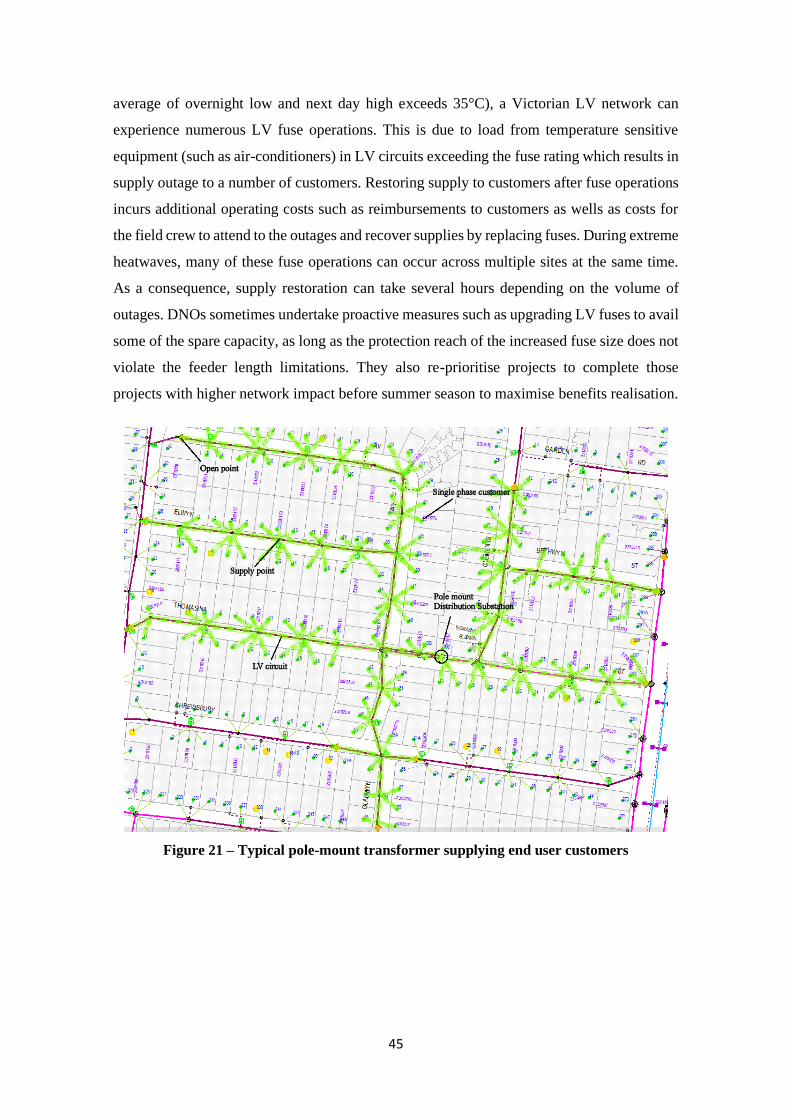
45
average of overnight low and next day high exceeds 35°C), a Victorian LV network can
experience numerous LV fuse operations. This is due to load from temperature sensitive
equipment (such as air-conditioners) in LV circuits exceeding the fuse rating which results in
supply outage to a number of customers. Restoring supply to customers after fuse operations
incurs additional operating costs such as reimbursements to customers as wells as costs for
the field crew to attend to the outages and recover supplies by replacing fuses. During extreme
heatwaves, many of these fuse operations can occur across multiple sites at the same time.
As a consequence, supply restoration can take several hours depending on the volume of
outages. DNOs sometimes undertake proactive measures such as upgrading LV fuses to avail
some of the spare capacity, as long as the protection reach of the increased fuse size does not
violate the feeder length limitations. They also re-prioritise projects to complete those
projects with higher network impact before summer season to maximise benefits realisation.
Figure 21 – Typical pole-mount transformer supplying end user customers

46
Figure 22 – Picture of a pole-mount transformer in suburban Melbourne
Figure 23 – Tap setting and nameplate of a 200 kVA pole mounted transformer
Unlike power transformers used in Zone Substations, distribution transformers do not
have OLTC devices, which means that they do not monitor or regulate voltage. They have
off-load tap changers with typically 7 steps (2 boost, 4 buck and 1 neutral) as shown in Figure

47
23 (left-side) where tap position 3 has been selected. These off-load tap positions provide the
ability to set the secondary voltage at 0.95-1.10 per unit (p.u.) with 2.5% increments by
adjustment of the local transformer turns ratio. Figure 23 shows a pole-mounted transformer
nameplate from the case network we have modelled (referred to as ‘Case Network 1’ going
forward) which has a 4% impedance rating, typical of those found of this size in Australia.
The typical transformer impedances along with X/R ratios for transformers used in Australian
distribution networks are shown in Table 5.
TABLE 5 – TRANSFORMER IMPEDANCES TYPICALLY USED IN AUSTRALIA AT 75°C [90]
Description Z (%) X/R ratio R (%) X (%)
25 kVA 3ph 22kV Pole-mount 3.3 3.00 1.04 3.13
100 kVA 3ph 22kV Pole-mount 4 4.00 0.97 3.88
200 kVA 3ph 22kV Pole-mount 4 4.12 0.94 3.89
315 kVA 3ph 22kV Pole-mount 4 4.36 0.89 3.90
400 kVA 3ph 22kV Pole-mount 4 5.33 0.74 3.93
350 kVA 3ph 22kV Pad-mount Kiosk 6.3 3.60 1.69 6.07
1500 kVA 3ph 22kV Pad-mount Kiosk 6.3 7.00 0.89 6.24
In LV distribution, off load tap changers are often the only form for voltage control
typically available to the DNO for LV. This is demonstrated in Figure 24 where the average
voltage position is lowered once the tap operation is complete. But manually adjusting
thousands of local transformers, one connection request at a time, is not an efficient exercise
and ultimately increases operating costs and hence tariffs. This is in contrast to HV, where
voltage support is provided by means of quadrature power supplied by synchronous
condensers (over-excited synchronous motors, on no load). In MV distribution, capacitor
banks provide leading PF, or a combination of thyristor-switched inductor/ capacitors
(STATCOM) provide leading and lagging PF.
Figure 24 – Average voltage lowers after tap down operation [96]
Four network components studied so far (transformers, tap position, MV and LV
lines) all have an effect on the overall voltage regulation bandwidth that ultimately dictates

48
voltage received at the point of customer connection. This bandwidth will be studied in more
detailed in the following section.
3.4. Voltage Regulation Bandwidth
From the point of view of LV planning, upstream voltage regulation is hence made
up of 5 network elements:
3.4.1. MV bus
MV regulation directly affects the voltages seen at distribution transformer and at
customer premises. Power transformers in Zone Substations have On-Load Tap Changing
transformers which continually adjust their tap positions (+/- single 1.25% tap) on the fly,
according to time of day, day of the week or consumption profiles of downstream load on
particular feeders. Additionally, utilities in Victoria are known to run dynamic voltage
management systems which can change power transformer tap based on the smart meter
voltages on the loads downstream of the power transformer. 2.5% contribution to voltage
regulation can be expected from the tap changes at the MV bus.
3.4.2. MV feeder to distribution transformer
DNO’s also implement wide-scale PF correction of medium-voltage (MV) feeders
using distributed capacitors. This significantly reduces the voltage drop along the MV feeders
and can raise voltages within the LV networks by approximately 1 to 4V on PF corrected
feeders.
Utilities are able to ascertain their MV feeder voltages with a fair degree of certainty
due to MV monitoring that is fairly prevalent. In Case Network 1, the total length of the MV
line to the supply Zone Substation is 5,896m. The current and voltage profile along the MV
feeder for one phase are shown below with 4.106A flowing from the Zone Substation to the
Case Network 1 transformer. Voltage seen at the primary side of the Case Network 1
transformer is given as 12.803kV line-to-neutral i.e. 22.175kV line-to-line. There is voltage
drop noticeable in the MV line since the voltage at the Zone Substation is 13.083kV line-to-
neutral i.e. 22.660kV line-to-line. This represents a voltage drop of 2.14% in the MV line at
this point of time. This can usually go up to 4% voltage drop in peak load 10% POE
(Probability of Exceedance) conditions and 1% voltage drop in light load conditions [82].

49
POE is the likelihood that a demand forecast will be met or exceeded. A 10% POE maximum
demand projection is expected to be exceeded, on average, one year in 10, while a 50% POE
forecast is based on average weather and is expected to be exceeded, on average, every second
year. Hence 3% contribution to voltage regulation can be expected in the MV feeder.
Figure 25 – MV feeder line-to-neutral voltage profile upstream of Case Network 1
Figure 26 – MV feeder current profile upstream of Case Network 1
3.4.3. Distribution transformer impedance to LV secondary
The internal winding resistance of the transformer also plays a role. Voltage drop
across the transformer terminals has been measured as ranging from 2.6% to 0.4% at a 125%

50
and 20% loading (of nameplate rating) respectively [82]. This study also used a transformer
with 4% impedance and a similar PF of 0.95. Hence, 2.2% contribution to voltage regulation
can be expected in the distribution transformer.
3.4.4. Distribution transformer tap offset
Localised voltage regulation issues are often resolved by distribution tap changes,
which typically occur in 2.5% single step changes as discussed previously. The overall
contribution to voltage regulation that can be expected from the 4 upstream network elements
is 10.2%. Since a total of 16% bandwidth (+10%/-6% as per Table 1) is available, this leaves
only 5.8% available bandwidth for downstream regulation.
3.4.5. LV mains feeder and service wire
LV networks are most likely to be constrained by the voltage deviation within them
as opposed to that as a result of the voltage deviation in the MV network. This is particularly
true on larger LV networks (i.e. overhead residential networks with large numbers of
customers in each circuit), since these will have much larger LV deviations. There are two
more downstream network elements within which voltage regulation will be experienced: the
LV mains feeder and the LV service wires. For the service wires, allowance for 1V voltage
rise and 1.3V voltage drop [82] is typical, which works out to be another 1% contribution to
voltage regulation. You hence have only 4.8% (11V) available bandwidth for LV mains
feeder voltage regulation. Every feeder will have different values for voltage drop and voltage
rise, and hence different allowable voltage headroom. We see typically 2.5% contribution to
overall voltage regulation from the LV feeder for a well-balanced circuit. But that depends
also on factors such as circuit impedance, PV penetration and coincidental peak load. When
calculating headroom in a feeder, it is an acceptable practice in Victoria to use V99 and V1
values to negate outliers, as discussed earlier.
TABLE 6 – TYPICAL VOLTAGE BANDWIDTH CONTRIBUTIONS IN LV FEEDER
Network Element Typical Contribution to Bandwidth
MV bus 2.5%
MV feeder 3%
Distribution transformer impedance 2.2%
Distribution transformer tap 2.5%
LV mains feeder < 4.8% (11V)
LV service wires 1%

51
As summarised in Table 6, there is only a small, finite bandwidth available to voltage
regulation in the LV grid, which is a challenge.
3.5. Consumption Data from Meters
Smart-meters installed in Victorian households give visibility of aggregate demand
at 5-minute or even 10-second intervals. Advanced Metering Infrastructure (AMI) data has
been used in previous studies for interruption reporting and statistics, fault indication, location
and in the case of very advanced meters, isolation in LV networks [97]. We will extend the
use of metering data to distribution network design by calculating voltage profiles when new
residents are connected onto the network model.
Figure 27 – Picture of an AMI meter installed in a suburban house in Melbourne
For our research, half hour interval metering data is available to us, which provides
the following information: -
• Date and interval
• kVAr and kW, either consumed or generated
• National Metering ID and Meter no.
• Register ID (with values E1 for load and B1 for PV)

52
Note this information can also be usually obtained by any householder through an
online request from the utility or retailer. National Meter Identifier (NMI) is a unique 10- or
11-digit number used to identify every electricity network connection point in Australia. This
is how retailers can identify a site’s electricity supply.
PART II – MODEL CONSTRUCTION
The second part of this chapter outlines the model of the real-world network used in
our research and the general analysis approach that utilities use for modelling network
components in distribution networks and power-flow simulation.
3.6. Software Tools
Having the ability to model PV and household loads in half-hourly intervals was a
key requirement in choosing a simulation tool for our research. Many commercial software
packages are available that can perform LV distribution network simulations. Some of the
commonly used ones are PSS®Sincal, MATLAB®SimPowerSystems, OpenDSS™,
ReticMaster™, PowerFactory™ and CYMDIST™. Performing simulations for both low and
high load scenarios as well as low and high solar irradiation times would be necessary.
But simulations for longer time periods may also be required due to other factors at
play. Impact on the network assets and voltage profile of the LV feeder is highly dependent
on customer usage patterns and phase imbalance as well. The simulation tool chosen should
not limit us to a snapshot of critical time periods only. And it should be able to perform time
series analysis (not dynamics or transients’ studies) for an entire year with relative ease and
speed. We would also require it to be inexpensive (preferably free to use for research
purposes) and computationally responsive. We have decided to use OpenDSS™ (Open
Distribution System Simulator™), an open-source software developed at the EPRI (Electric
Power Research Institute) [94], [98]. The default load flow algorithm used in OpenDSS is the
current injection method, based on Newton-Raphson technique for solving the distribution
system. Accordingly, the load flow analysis as a part of the tool is based on the current
injection method. The relevant details can be found in OpenDSS manual [99]. The only overt
limitation of this software for us is that it does not allow simultaneous modelling or load flow

53
for more than one distribution transformer at a time. This does not affect us as looped
networks are not considered in our research.
In OpenDSS, a user has to create multiple files that can store various components of
a distribution system model. Files are required for the node X-Y coordinates, line codes, line
data, distributed generation data, transformer data and the load model. Shown below is an
example of an 8 bus LV network, its various components and how they are defined in
OpenDSS. LV voltages are measured relative to the secondary transformer LV busbar at A.
Figure 28 – Example of an 8 bus LV network [100]
In the above figure, Vsource is the voltage source at the node SourceBus. TR1 is the
transformer with the fixed turns ratio. Lines 1 to 5 are overhead or underground lines, the
physical line data for which are defined in the line data file. Loads 1 to 4 data and PV 1 to 2
data are defined in the load and generator files. These include magnitude, phase and type of
load and PV. Appendix C contains details on the OpenDSS code and a couple of output plots.
The OpenDSS software comes with a Component Object Model (COM) and hence
interacts well with MATLAB®, a well-known coding platform, used in our work for post-
processing. MATLAB has a good reputation of being easy to use amongst industry
professionals and researchers alike. Appendix C also contains the MATLAB code written for
invoking our OpenDSS model and running the power flow for one year’s worth of data.
3.7. 22-Bus Unbalanced Distribution Network
In OpenDSS, X/R of the line was obtained from the utility and conductor
manufacturer, instead of any assumed values. The span lengths (distance between successive

54
poles or LV busbars), the 4-wire geometrical configuration data (such as height of LV
attachment on pole and length of LV cross-arm), the transformer size, transformer
impedance and phase information for each customer were all modelled as found on site.
Half-hourly demand data for a whole year (June 17, 2014 12.30am to June 17, 2015
12.00am) for all the 54 residences being serviced by the transformer were also used from the
interval metering data provided by the DNO. The PF at each half-hour interval was also
available. Hence the load reactive power could be calculated, instead of any assumptions
required. The data-set’s peak demand (130 kW or 138 kVA) was on 21st February 2015. The
local maximum temperature on this day according to the Bureau of Meteorology was 37°C
and the overnight low was 19°C. This makes sense because when the maximum temperatures
exceed 35°C, the air-conditioning load is a major cause of peak demand in Victoria.
A geographical representation of the network can be seen in Figure 29. The blue
circles represent the poles (or nodes), and the red triangle represents a 3-phase 200 kVA
22kV/433V Dyn11 pole-mounted transformer at bus 1. Span 1 between bus 1-2 is modelled
as a 1m length of cable connecting the transformer secondary to the overhead wire. This
network splits into two different branches at bus 2 (east and west) at the outset. Bus 2 to 9 is
the radial west circuit and Bus 2 to 16 is the east circuit. The north-east branch of bus 17 to
22 connects onto bus 11. Span lengths are typically around 45m as shown in Appendix A.
There are 8 houses on this network with PV panel installations. Buses 4, 7, 13, 14, 19 and
22 have PV connections. The thickness of the blue lines represents the typical amount of
power flowing into the overhead lines at a particular timeslot, which in this case is June 17,
2015 12.00am. The service wires are not modelled in our research and are hence not shown.
A snapshot of the United Energy GIS is shown in Figure 30. Since this is aligned to
true north, it is oriented differently compared to the OpenDSS representation. The service
wires are visible in the GIS snapshot. The transformer pole has been highlighted.
Figure 29 – Spatial representation of multiple branched radial LV network diagram
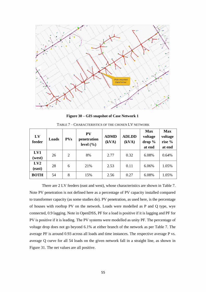
55
Figure 30 – GIS snapshot of Case Network 1
TABLE 7 – CHARACTERISTICS OF THE CHOSEN LV NETWORK
LV
feeder Loads PVs
PV
penetration
level (%)
ADMD
(kVA)
ADLDD
(kVA)
Max
voltage
drop %
at end
Max
voltage
rise %
at end
LV1
(west) 26 2 8% 2.77 0.32 6.08% 0.64%
LV2
(east) 28 6 21% 2.53 0.11 6.06% 1.05%
BOTH 54 8 15% 2.56 0.27 6.08% 1.05%
There are 2 LV feeders (east and west), whose characteristics are shown in Table 7.
Note PV penetration is not defined here as a percentage of PV capacity installed compared
to transformer capacity (as some studies do). PV penetration, as used here, is the percentage
of houses with rooftop PV on the network. Loads were modelled as P and Q type, wye
connected, 0.9 lagging. Note in OpenDSS, PF for a load is positive if it is lagging and PF for
PV is positive if it is leading. The PV systems were modelled as unity PF. The percentage of
voltage drop does not go beyond 6.1% at either branch of the network as per Table 7. The
average PF is around 0.93 across all loads and time instances. The respective average P vs.
average Q curve for all 54 loads on the given network fall in a straight line, as shown in
Figure 31. The net values are all positive.

56
Figure 31 – Average P and Q for all households
The cumulative active and reactive power at the distribution substation are shown in
Figure 32. There is no noticeable trend except that the real and reactive power components
are directly proportional. The reactive power is much lower than the real power, which
indicates a low number of reactive power devices and/or a low correlation between when
devices that consume/ export reactive power (e.g. washing machines) are used [56].
Figure 32 – Cumulative P and Q load downstream of substation
All values are positive downstream of the transformer which indicates that there is
no reverse power flow in this network due to reasonably low PV penetration. For the east
circuit, the active power elements do show up with negative values, due to the higher PV
penetration in this circuit.

57
Figure 33 – Cumulative P and Q load in the east circuit
Figure 34 – Cumulative P and Q load in the west circuit
3.8. Conductor Impedance Characteristics
The overhead bare LV mains conductor modelled, as provided by the utility, is
19/3.25 AAC (interpreted as 19 strands of 3.25-inch diameter of All Aluminium Conductor)
with r = 8.125mm. At 65°C, R is calculated as 2.196 mΩ/km. We have calculated the GMR
as 0.7788 x 8.125 = 6.32775mm. The GMD depends on the distance between the individual
phases. In our research, we have used GMD for the 2100mm cross-arm, as found on site.
Phase-to-phase separation of 600mm is hence used in the calculation of GMD:
𝐺𝑀𝐷 = √600 x 1300 x 19003
= 1140.11𝑚𝑚 and hence X = 326.1 mΩ/km.

58
3.9. Model Inputs from Meter Data
The other piece we required in order to carry out the simulation was interval-meter
data. Table 23 in Appendix B provides a snapshot of the meter data made available to us. The
meter number is the serial number of the meter itself. There are 365 x 48 rows for each
household. If a household has PV, there are a further 365 x 48 rows with PV power generated
for those houses.
3.10. Micro Embedded Generator Connection
Most of the voltage rise within the grid is a result of rooftop PVs, which is the most
common type of micro embedded generator. The ability to represent PV inverter with a
realistic solar profile is critical. We have obtained solar generation data from a utility for the
8 households on the network; and have modelled the PV units as power sources.
Figure 35 – Average annual PV generation profile
Solar generation data, much like the consumption data, is available in half-hour
intervals. It hence does not show transient fluctuations due to passing clouds, etc. The 8
profiles are all different due to the difference in panel size, orientation of roof and shading.
The average profile of the 8 profiles, over the course of the whole year is shown in Figure 35.
It shows peak generation around 12.30pm, with almost all of the solar power generated
between 8am and 5pm when averaged across all 4 seasons.

59
3.11. Data Visualisation
Once the model has been set up, we then run the simulation, Figure 36 shows the
voltage profile at Bus 22, which is one of the three LV feeder extremities of the case network.
This plot has been obtained from simulation in OpenDSS using voltage at Line 21, which
refers to the span from Bus 21 to 22, and the voltages shown at load end. The x-axis is time
elapsed from June 17, 2014 (referred to as Day 1) to June 16, 2015 (Day 365). The three
phases have been shown separately, with the white phase voltage shown in black.
Figure 36 – Voltage profile at Bus 22
The unbalance on the line becomes apparent as the white phase has the greatest
voltage drop and seems to be the heaviest loaded.
Figure 37 has been obtained at Bus 1 from simulation in OpenDSS, and shows
aggregated consumption data from all the different households as seen by the transformer.
The graph confirms that white phase is the heaviest loaded and hence we confirm an inverse
correlation between voltage and demand. As before, the x-axis reflects the day of the year
from June 2014 to June 2015. As can be noticed, the summer months of January and February
have some peak load days but do not reflect the highest peak aggregated load in the year. But
usually in Victoria, the air conditioning load in summer far exceeds the winter load from
heating which is not noticed in above network plot for July-August. It can thus be surmised
that this was a mild summer.

60
Figure 37 – Demand profile at the Substation
Figure 38 shows the time series voltages at Bus 9 on a hot day. Bus 9 is one of the
feeder extremities in this network. We see that the voltage drop maxima and minima at Bus
9 generally coincide with the transformer load maxima and minima respectively.
Figure 38 – Load and voltage profiles for a high demand day
The peak load is around 5.30pm which is when householders return to their homes
and turn on air-conditioning loads and other appliances. The rest of the times will include a
baseload powering fridges and freezers and other small electronic equipment.

61
The maximum and minimum voltage at the load end of each line are shown in Figure
39. 4 points per line are shown: the highest and lowest voltage in the year and the V99 and
V1 as well. The three phases have not been shown individually in this graph. Since line 9 and
line 2 are geographically close to each other, the voltages are fairly close as well. Likewise,
for line 11 and line 16. This graph is useful for determining the headroom available for
additional load or PV connection on each line. If calculating the headroom for line 13 for
example, you would first allow for 1V voltage rise and 1.3V voltage drop in the service wires
which haven’t been modelled in OpenDSS. You would then have no further leeway in voltage
drop since you will have reached the lower limit of 216.2V as specified in Victorian
regulations. But for voltage rise you would have 27.7V (= 253 - 224.3 - 1) of headroom
available. There would have to be certain allowance made for the upstream voltage
regulation. A typical allowance for MV variations as shown previously is 23.5V (or 10.2%).
Total headroom available would hence be 4.2V. This can be adjusted either for voltage drop
or voltage rise by specifying a tap setting in OpenDSS. The tap setting in OpenDSS used in
these simulations is 0.975p.u. This translates to a starting voltage of 0.975 x 230 = 224.25V.
The starting voltage of line 1 does not line up with 230V for this reason. Figure 39 suggests
that the transformer may be tapped up in practice to avoid any voltage drop violations.
Figure 39 – Voltage at load end of each line of Case Network 1
All the lines are experiencing some level of voltage rise. Some of the voltage rise is
due to PV but some of it is due to presence of single-phase loads that haven’t been distributed
in a balanced way amongst the phases along that branch. This can be verified if we plot the
V1 and V99 using the average of the three phases at each line.

62
Figure 40 – 3-phase average voltage at load end of each line of Case Network 1
A lot of the voltage rise is now not present as shown in Figure 40. This is why relying
on literature that takes only balanced networks into account should be met with
circumspection. The maximum voltage drop seen is much lower than that seen in Figure 39.
This gives an indication why phase imbalance is so crucial for a complete picture on voltage
regulation analysis.
In this chapter, we have looked at the various components of the electricity
infrastructure used to deliver power to homes. We then looked at all the contributors to
voltage regulation and the available bandwidth for LV mains voltage rise or drop. In part II
of this chapter, we focussed on finding the right software tools for our research. We then
chose a case network, part of the one of the worst performing MV feeders for voltage
excursions, from a utility in suburban Melbourne. We then detailed the technical calculations
required to model the network. We then ran the simulation and analysed the results for
demand vs. voltage.

63
CHAPTER 4 – PARAMETRIC MODELLING
FOR MACHINE LEARNING
In this chapter, we take the traditional method given by equation (16) repeated below,
as a starting point and expand it further so we obtain a parameter that captures the effect of
solar connections on voltage regulation.
We refer to the combined load diversity and unbalance factors DF and UF as Load
Correction Factor (LCF) for the remaining part of the thesis. Note the traditional method does
not consider the reverse power-flow from prosumers i.e. residences with solar PV panels.
These residences back-feed power into the LV grid, causing voltage rise. In order to capture
this, a new parameter, called Solar Correction Factor (SCF), is incorporated in Equation (16)
to counter the traditional voltage drop. The traditional method is hence revised to form a new
equation including SCF, NPV and PPV:
There is insufficient evidence that empirical methods traditionally used to obtain LCF
still hold up given the changing consumption patterns and household device efficiencies, etc.
What we would like to do is develop a new method to that forecasts future voltages from a
given sequence of historical observations, i.e. a time series. Historically, time series
𝑉𝐿 = 𝑉𝑆 − 𝑈𝐹 x 𝐷𝐹 x (𝑅𝑐𝑜𝑠𝜃 + 𝑋𝑠𝑖𝑛𝜃
𝑉𝑆
) 𝐴𝐿𝑁 (16)
𝑉𝐿 = 𝑉𝑆 − (𝑅(𝐿𝐶𝐹 x 𝑁 x 𝑃𝐿 − 𝑆𝐶𝐹 x 𝑁𝑃𝑉 x 𝑃𝑃𝑉)
𝑉𝑆) 𝐿 − (
𝑋(𝐿𝐶𝐹 x 𝑁 x 𝑄𝐿)
𝑉𝑆) 𝐿 (32)

64
forecasting has mainly been studied in statistics and econometrics. In the last decade though,
machine learning has become one of the most active areas of predictive modelling and
research. It involves creating algorithms that can automatically learn from data. We propose
to use a standard machine learning algorithm called non-linear regression to train the LCF
and SCF. The methodology has been shown in my conference paper [1] to be appropriate for
our use, as we can define the general function form and estimate parameters from the data.
We seek to approximate a function, given a finite sample of training instances, similar to
supervised classification. This methodology will allow updating of well-established voltage
estimation methods.
The secondary reason of proposing this methodology is due to the nature of question
being posed: “Given the power consumption data for each household, how much further
voltage drop or rise is a new connection expected to cause on the network?” The intention is
to learn what makes the voltage profile behave a certain way from the training data. Using
those learned characteristics, the algorithm should then produce the new voltage profile based
on new input data i.e. be able to predict the voltage. The learned structure should hence apply
well beyond the training data and help prove that machine learning is an appropriate tool to
forecast load voltage and that data analytics can have many more applications in power
systems. This will form the basis of our solution.
4.1. Background
Since we have already defined the general function form, let us have a look how
machine learning can be applied. Depending on their output, machine learning models can be
classified as regression (the target variable is continuous), classification (the target variable
is categorical), and others like clustering (often unsupervised), probability density estimation,
and dimensionality reduction [101]. Machine learning has grown in popularity in the last few
years, and it is being used today for data analysis in the manufacturing industry, healthcare,
financing, etc. This is largely due to its superior performance in making predictions. If the
objective of machine learning is not very obvious (not a well-defined problem), it is called
unsupervised learning. This is useful when only patterns are being sought, without much
information beforehand on what they might look like. Supervised Learning with the other
hand, is when each data point comes with a label or a response. This can also know as the
output or the dependent variable in statistics. In an unsupervised environment, the labels are
missing. At a high level, supervised learning is function approximation.

65
Figure 41 – Unsupervised Learning and Supervised Learning [102]
In classification, labels are from a fixed, finite set, for e.g. 0 and 1 for binary
classification. Labels that have a continuous numerical range lead to a regression problem
[102]. Regression allows a set of data points to be estimated by a curve described by an
estimator 𝑓(𝐱). The main purpose being to construct such a curve that accurately predicts
unrecognised data and minimises the regression error. The challenge is to find an estimator
(or estimation function) so that the predicted value is unbiased and consistent i.e. is as close
to the correct value as possible. Estimation functions generally fall into the two categories:
linear and non-linear. Linear regression is used when the independent variables x are related
by a linear relationship. Note due to complexities brought about the non-linear relationship
between demand and voltage, we cannot use linear regression, and hence propose non-linear
regression. Non-linear regression function 𝑦𝑖 = 𝑓(𝐱𝑖, 𝛃) represents the relationship between
a vector of independent variables, x (inputs or predictors), and its associated observed
dependent variables, y (response variables). The function f is nonlinear in the components of
the vector of parameters β (regression coefficients), but otherwise arbitrary.
Next, a training set is created: 𝐱𝑖 ∈ 𝐑, m, y𝑖 ∈ 𝐑, i= 1,...,m.
This is a collection of labelled examples that a supervised learner can train on before
it can predict labels of instances. Our training set is defined as containing of 3 input variables
(QL, PL, PPV) and 1 output target or response variable (VL) for each time instance. The input
variables are the active and reactive power consumed and the active power generated at each
bus of the network. The response variables are the load voltage for each bus and have been
obtained from simulation in OpenDSS.

66
With our training set defined, we pass it into a learning algorithm which creates a
function. The function will be used to take an input and output a prediction based on that
input. This may be interpreted as black box process wherein we have no visibility of what
assumptions the function is internally making to make the predictions. Hence what we would
also like, in addition to the function, is visibility of SCF and LCF parameters determined by
the learning system, so that they that can be reconciled to existing voltage drop or voltage
rise calculation practices such as excel spreadsheets modelled on Equation (32).
For a well posed learning problem, we will need to define a performance measure.
This will allow us to measure the accuracy with which predictions are being made. This is
usually done by calculating the loss function 𝐿, which is done by comparing the model’s
predictions to the test data (or the ground truth). For regression, this is done by calculating
the Mean Squared Error (MSE). MSE gives an estimate of the variance of the error term.
Different machine learning tools look to minimise the MSE or cost function of the regression.
The vector of coefficients returned in β hence minimises the least squares equation. We define
𝐿 as:
Given a loss function, training error (or empirical risk) is defined as:
An ‘off-the-shelf’ function in MATLAB called ‘fitnlm’ is used to perform this
analysis, which executes the Levenberg-Marquardt (LM) least squares algorithm [103] to
minimise the MSE between the predicted and the observed responses. This will be used to
evaluate the parameters that lead to the least loss on the training set.
A test set is also created: 𝐱′𝑖 ∈ 𝐑, m’, y′𝑖 ∈ 𝐑, i= 1,...,m′
4.2. Non-Linear Regression Fit – Implementation
Before the machine learning process can be carried out, simulations in OpenDSS and
post-processing in MATLAB need to be completed. Simulation of the case network in
𝐿 = ∑[𝑦𝑖 − 𝑓(𝐱𝑖, 𝛃)]2𝑚
𝑖=1
(33)
𝐸 =1
𝑚∑ L(𝑦𝑖, f(𝐱𝑖, 𝛃))
𝑚
𝑖=1
(34)

67
OpenDSS is carried out under 2 scenarios: one with the distributed generation and one
without. The time-series PL and QL for each line is taken from the simulation without PV. But
the time series records of variable VL will be taken from the simulation with PV. This is done
because the time-series PL and QL line data available in the first simulation was a net load
minus PV output, and not the true consumer load.
Variable VL used for training is not the average of the 3-phase voltages; but is taken
as the minima or maxima of the 3, depending on time of day. From 11am to 2:30pm, the
maxima of the phase voltages are used. This would train the model for voltage rise as demand
is low and solar output is high. For 6:30am to 9am and 3:30pm to 9pm, the minima of the
voltages are used. Data from these 18 half-hour intervals would train the model for voltage
drop since load is high at these times. The rest of the 22 half-hour intervals are not used for
training as voltage excursions in a residential network are not noticeable during those times.
Next, the training and test data are demarcated as different halves of the line voltage
data obtained. Training Set A contains the data for the first half of the year. The rest of the
data constitutes the Test Set A. These sets each contain 99,645 points for VL, i.e. 4,745 data
points for each bus. The first 4,745 data points are for bus 2, then the next 4,745 data points
are for bus 3 and so on.
We also establish Test data that are obtained from networks with different number of
residential connections than Case Network 1. Training Set B contains two collections of data
– one with simulated voltages from Case Network 1 with 20 fewer residences; and one from
the Case Network 1 with 20 more residences. There is a total of 398,580 data points taken for
VL i.e. 26 half-hour interval data points for 365 days for 21 busbars, twice over. The loads
removed or added are chosen at random locations amongst the different nodes. The
consumption profile of each of the added loads is taken as an average consumption profile of
the 54 residential profiles. Test Set B is created with the expected voltages from the
simulation of Case Network 1 for the whole year. Hence, it has 199,290 data points (m’). This
will be used to calculate the MSE between predictions.
Next the assessments for SCF and LCF for each bus are done via non-linear regression
through an iterative procedure. This is a machine learning technique that fits a non-linear
model specified by Equation (32) to variables PL, PPV, QL stored in a dataset array for each
time instance. We will be using the ‘fitnlm’ function in MATLAB again as it creates a
least-squares fit of the response to the data, minimising the empirical risk, and returning a
non-linear model.

68
For the first node though, Equation (32) is further refined so that VS is assumed as
230 x tap. This is so that the starting voltage can be calibrated with upstream voltage
regulation in the MV line. Once the tap value has been obtained for node 1, it is no longer
used for training of downstream node voltages. The parameter tap in OpenDSS has been
specified as 0.975p.u. This translates to a starting voltage of 0.975 x 230 = 224.25V.
The initial guesses for the parameters are taken as 1. VS is taken from predicted data
for the upstream node. Therefore, topology of the network is also stored as an input i.e. for
each bus, the upstream busbar number is stored. This is so that the predicted load voltages of
the upstream bus can be used as source voltage of the next bus.
4.3. Testing Data and Validating Predictions
Once a trained model, tap setting for the first bus and specific LCF, SCF for every
bus are created, then voltage for each bus of the case network for each time stamp can be
generated. This is done here using the ‘predict’ function in MATLAB. This function uses
parameters belonging to the case network (QL, PL, PPV) and response variable VL. VS is taken
from predicted data for the upstream node. The same topology is used as the training network
since that does not change. The results for VL are then compared to simulation results as well
as results from Equation (16). Since the case network is in Victoria, Australia, an LCF with
k = 12 is used in this research, which is as per local power industry guidelines [91]. Since
Equation (16) provides a solitary value for voltage instead of a time-series of voltages, it is
compared to 99-percentile values for each bus. The V1 values are not used for comparing
voltage rise since Equation (16) does not calculate voltage rise. The RMSE difference in
corresponding V1 and V99 values of the predicted and simulation voltages is calculated. The
MSE of the fitted model is returned as a scalar value. The expected voltage results are from
Test Set B, but could also be readings from smart meter voltage data, were they available.
The advantage of using non-linear regression-based machine learning is that LCF and
SCF parameters can be obtained and reconciled to existing voltage drop or voltage rise
calculation practices such as excel spreadsheets modelled on Equation (32). This is important
to create a grey box model that utilises machine learning and also presents the parameters to
engineers and provide visibility of the in-built assumptions of the model. A grey box model,
𝑉𝐿 = 𝑡𝑎𝑝 x 𝑉𝑆 − (𝑅(𝐿𝐶𝐹 x 𝑁 x 𝑃𝐿 − 𝑆𝐶𝐹 x 𝑁𝑃𝑉 x 𝑃𝑃𝑉)
𝑡𝑎𝑝 x 𝑉𝑆) 𝐿 − (
𝑋(𝐿𝐶𝐹 x 𝑁 x 𝑄𝐿)
𝑡𝑎𝑝 x 𝑉𝑆) 𝐿 (35)

69
as used here, is a model where the engineer has limited knowledge over the internal workings
of the methodology but doesn’t face a steep learning curve. The grey box is a blend of black
box and white box techniques. This has advantages when compared to a white box model,
such as static load flows, where the user requires full knowledge of the internal workings of
the application and also faces a time-consuming and exhaustive process. A grey box helps
create an explainable model which is very important in industry. The methodology becomes
easier to explain and implement which gives it a strong advantage when compared to other
analytical models. Section 4.5 discusses how we measure the performance of this grey box
model compared to status quo.
Figure 42 – Workflow for machine learning and validating predictions (grey box)
In the next section, we show a classical black box model for comparison purposes.
As defined here, the black box model is where internal behaviour is not known or understood
by the user. While performance of a black box model may potentially be better, it is not
explainable to engineers and electricity industry professionals and is not expected to find
acceptance in industry at large. A binary regression decision tree model from the 1980’s is
sufficient for the purposes of comparison. Finding better black box models such as algorithms
based on Artificial Neural Networks, k-nearest Neighbour, the Bayesian algorithm or
classification using Support Vector Machine is beyond the scope of this work.

70
4.4. Decision Tree
If we had very little knowledge or assumptions beforehand about how the different
variables are related, it becomes more of a data-mining type question. Decision tree models
have been considered suitable for this task. The purpose of the analyses via tree-building
algorithms is to determine a set of ‘if-then’ logical (split) conditions that lend themselves to
not only classification but also permit accurate predictions in regression problems. Tree
methods are non-parametric (and nonlinear) supervised machine learning algorithms with a
tree-like structure with its root node at the top. Each fork is a split in a predictor variable and
each node at the end has a prediction for the target variable. Note other approaches such as
neural networks can also solve regression problems, but have not been considered here.
The classical standard Classification and Regression Trees (CART) algorithm
developed by Breiman [104] is used here. This algorithm may be referred to as “decision
trees”, but is referred to as CART on some platforms like R and MATLAB. CART does not
require any special data preparation or implicit assumptions, other than a good representation
of the problem. It consists of 2 kinds of decision trees: -
• Classification Trees: A classification tree is an algorithm where the target variable
is fixed or categorical. The algorithm is then used to identify the “class” within which
a target variable would most likely fall. This is usually a binary split i.e. for two
classes that are mutually exclusive, the classification tree will split the data based on
homogeneity.
• Regression Trees: A regression tree refers to an algorithm where the target variable
is continuous and the algorithm is used to predict its value [105]. A regression model
is fit to the target variable using each of the independent variables.
CART is one of the oldest and most fundamental algorithms of machine learning.
Given a new input, the tree is traversed by evaluating the specific input started at the root
node of the tree. It splits each branching node of the binary tree based on the values of the
predictors. Essentially, a learned binary tree partitions up the input space based on the
predictors and response variable from the input data. Once the predictors (QL, PL, PPV) and
response variable (VL) have been defined, the next step is to choose the split points on those
variables to create a suitable tree. The top few nodes on which the tree is split are the most
important variables within the set. Feature selection in CART gets performed automatically
which is an advantage. These split points will divide the input space using an approach called
recursive binary splitting. This is a numerical procedure where all the values are lined up and

71
different split points are tried and tested using a cost function. The split with the lowest cost
is selected. The cost function is the sum of MSE across all training samples that fall within
the space. Let 𝑦𝑖 denote the output for the training sample i and 𝑦 denote the prediction for
observation i, i = 1,...,m. The following least squares equation is formed with the most
accurate prediction being the prediction with the minimum cost (smallest variance or error):
This process is continued recursively. This algorithm is hence a very performance
heavy process. It is executed using the ‘fitrtree’ function in MATLAB here. The depth
of the tree should also be decided but ‘fitrtree’ grows deep decision trees by default. The
average number of splits is between 14 and 15. One can grow shallower trees to reduce model
complexity. Similar to previous function, one can use the ‘predict’ method to make
predictions. The following least squares equation is formed for predictions made on the test
set:
Figure 43 – Workflow for machine learning and validating predictions (black box)
𝐶 = ∑1
𝑚[𝑦𝑖 − 𝑦]
2𝑚
𝑖=1
(36)
𝐶′ = ∑1
𝑚′[𝑦𝑖 − 𝑦]
2𝑚′
𝑖=1
(37)

72
4.5. Validation Calculations
Once the predictions have been completed, three sets of calculations are performed
for validating them:
• RMSE between prediction and simulation voltage data points across all times and for
all nodes. This will help decide overall how well is the learning algorithm able to
predict load bus voltages provided a set of inputs.
• RMSE between predicted V1 percentiles and simulation V1 percentiles for all 21
nodes. This will help determine how far or close the predicted voltage drop is to the
actual values. This is an important metric as the utility is able to determine its appetite
for risk based on this. As long as the predicted V1 does not exceed allowable limits,
the utility should be able to keep adding more connections onto the network without
any augmentation expenditure.
• RMSE between predicted V99 percentiles and simulation V99 percentiles for all 21
nodes for voltage rise. Similar to above, this will help the utility gauge whether or not
to allow more prosumers onto the LV circuit.
From these three calculations, the black box and grey box models can be easily
compared to ascertain which provides better results.
Next, one additional calculation is performed for RMSE between the simulation V99
and the voltage drop provided by traditional methods at each node. This will help answer
whether the established methodologies fare better than our proposed methodology; and will
also provide an insight into whether a utility would have unwittingly refused to add
connections onto the network using established methods. For this purpose, we first create an
excel model of Equation (16). We run voltage drop calculations for the LV feeder, storing the
voltages at each node. These are then compared to the ‘ground truth’ simulation voltages. The
ground truth or the expected voltage results are from Test Set B, but could also be readings
from smart meter voltage data, where available. Note, the established methods do not provide
voltage rise values. Hence, no direct comparison can be formed between the proposed method
and the established ones.
For added functionality, in the excel models created above, we then use new values
of LCF and SCF. Instead of the empirically developed methods from Equation (16), we use
variables provided by the non-linear regression learning. This will help highlight the

73
differences in the voltage calculations from the traditional vs. regression models for each bus.
3 calculations will be carried out in this regard:
• RMSE between V99 of the new method using LCF, SCF and the V99 from the
simulation for each bus;
• RMSE between V1 of the new method using LCF, SCF and the V1 from the
simulation for each bus; and
• RMSE between simulation V1 and traditional voltage drop methods for each bus.
In this chapter, we reviewed the methodology used. This includes expanding the state-
of-the-art to create a parameter that can capture the effects of solar connections on feeder
voltage. We take a time series of voltages and propose a learning algorithm to fit a non-linear
function to approximate the parameters. We train voltage regulation parameters to forecast
voltage drop and rise along LV feeders with new connections; thereby creating better models
for predicting LV feeder voltages from given household demand. We also detail a black box
model which uses CART as the learning algorithm. In the next chapter we will look at the
performance of both algorithms and verify the results.

74
CHAPTER 5 – RESULTS AND DISCUSSION
5.1. Case Network 1
Thus far, simulation data is analysed and used for training and testing the parameters
using MATLAB as the main evaluation tool. In this chapter, the results of the predicted V99
and V1 are plotted; and the results from the machine learning algorithms are explained. First,
the results from Training Set A will be shown using the LM algorithm. This will be compared
with results from the CART algorithm. Next, the results from Training Set B will be shown
using the LM algorithm, and then compared to the results from the CART algorithm. Then,
new voltage drop and voltage rise calculations will be shown using the LCF and SCF from
the non-linear regression, as explained before. Then we will focus on results from a second
study done using a network of high level of PV penetration. This sensitivity check will
validate our methodology. We will be continually discussing our findings throughout this
chapter.
5.1.1. Learning and Testing on Training Set A – LM Validation
Machine learning is said to be valid if the error calculated for training and testing on
the same data set is zero or minimal. We perform our validation test on training Set A, first
using the LM algorithm. The results are shown in Figure 44. We see that it is a congested plot
of nearly 100,000 data points both from the simulated (blue) and predicted (yellow) data sets.
It is not easy to show if the predictions are matching the training data. Hence, we also show
the 1-percentile and 99-percentile from the data sets for each line voltage in red and black.
These are showing close alignment as we are training and testing on the same data set. We
then also overlay the traditional method Volt-Drop (VD) on the same graph and we see it is

75
diverging remarkably from the simulation data. This underscores the point that the traditional
method is not a reliable measure of the ground truth.
Figure 44 – Learning and Testing on Training Set A using LM
In the interest of clarity, we have replotted Figure 44 showing just the 1-percentiles
and 99-percentiles of test set and predictions. A very close match is now visible in Figure 45.
Figure 45 – Learning and Testing on Training Set A using LM replotted
West circuit (1) East circuit (2) East circuit (3)

76
The overall RMSE is 1.11V for all data points with the LM algorithm which indicates
a very good match indeed. For reference, the RMSE difference in the traditional method and
the simulation for voltage drop is much higher at 9.53V. The RMSE difference in predicted
and simulation 99-percentiles (voltage rise) for each line voltage is 0.44V and 1-percentiles
(voltage drop) for each line voltage is 1.07V.
5.1.2. Learning and Testing on Training Set A – CART Validation
To validate the CART algorithm, the same methodology is applied and the same data
set is used. As shown in Figure 46 and Figure 47, much better results are achieved and the
performance superiority of CART becomes visible. This makes intuitive sense since we are
testing on the same data set we trained the algorithm on. The overall RMSE is 0.8V for all
data points with the LM algorithm which is exceptionally small. The RMSE difference in
predicted and simulation 99-percentiles (voltage rise) for each line voltage is 0.15V and 1-
percentiles (voltage drop) for each line voltage is 0.10V. This is summarised in Table 8.
Figure 46 – Learning and Testing on Training Set A using CART

77
Figure 47 – Learning and Testing on Training Set A using CART replotted
TABLE 8 – COMPARISON OF RMSE (V) – TRAINING AND TESTING ON THE SAME DATA SET
Algorithm
/ Set
RMSE
between all
prediction and
simulation
voltages
RMSE
between
predicted V99
and simulation
V99
RMSE
between
predicted V1
and simulation
V1
RMSE
between
simulation V1
and traditional
voltage drop
LM / Set A 1.11 0.44 1.07 9.53
CART / Set A 0.80 0.15 0.10 9.53
5.1.3. Learning with Training Set A and Testing on Test Set A using LM
We have tested the two algorithms used in our work and they are performing very
well which was expected when training and testing on the same data set (first half of the year).
Next, we train using the LM algorithm on Training Set A (first half of the year) and test on
Test Set A (second half of the year).
The results are shown in Figure 48. The x-axis has 99,645 points, i.e. one for each
timestamp over the 6 months. The entire predicted data set is also plotted along with the upper
and lower percentiles. Figure 49 shows only these percentiles for expected line voltages from
the simulation and the percentiles for the predicted voltages. The overall RMSE is 1.22V for
all data points with the LM algorithm which indicates a very good result given we are training
on one half of the year and testing on the other half. The RMSE difference in predicted and
expected 99-percentiles (voltage rise) for each line voltage is 0.61V and 1-percentiles
(voltage drop) for each line voltage is 1.87V.

78
Figure 48 – Expected and predicted results of Set A using LM
Figure 49 – Learning with Training Set A and Testing on Test Set A using LM
Table 9 shows the average LCF and SCF obtained for each line from the non-linear
model fit. The LCF from the traditional method is also shown. The SCF created for PVs
provides a higher order of flexibility that the traditional method does not have. Since the first
span from bus 1 to 2 is modelled as a 1m length of cable, its results are not included in the
average. Line 1 is used primarily in the LM algorithm to train the transformer tap parameter,
the prediction for which is 0.975p.u. This matches the turns ratio specified in the simulation.
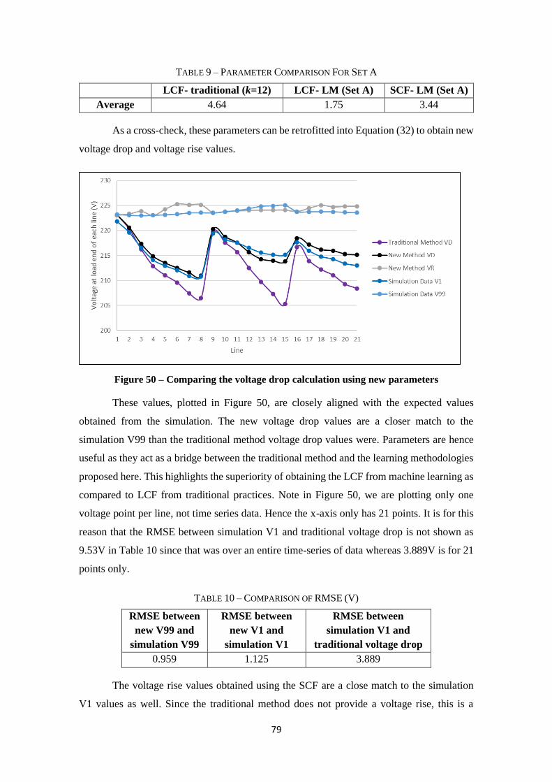
79
TABLE 9 – PARAMETER COMPARISON FOR SET A
LCF- traditional (k=12) LCF- LM (Set A) SCF- LM (Set A)
Average 4.64 1.75 3.44
As a cross-check, these parameters can be retrofitted into Equation (32) to obtain new
voltage drop and voltage rise values.
Figure 50 – Comparing the voltage drop calculation using new parameters
These values, plotted in Figure 50, are closely aligned with the expected values
obtained from the simulation. The new voltage drop values are a closer match to the
simulation V99 than the traditional method voltage drop values were. Parameters are hence
useful as they act as a bridge between the traditional method and the learning methodologies
proposed here. This highlights the superiority of obtaining the LCF from machine learning as
compared to LCF from traditional practices. Note in Figure 50, we are plotting only one
voltage point per line, not time series data. Hence the x-axis only has 21 points. It is for this
reason that the RMSE between simulation V1 and traditional voltage drop is not shown as
9.53V in Table 10 since that was over an entire time-series of data whereas 3.889V is for 21
points only.
TABLE 10 – COMPARISON OF RMSE (V)
RMSE between
new V99 and
simulation V99
RMSE between
new V1 and
simulation V1
RMSE between
simulation V1 and
traditional voltage drop
0.959 1.125 3.889
The voltage rise values obtained using the SCF are a close match to the simulation
V1 values as well. Since the traditional method does not provide a voltage rise, this is a

80
significant improvement over the state-of-the-art. Hence, we can see that the LM algorithm
has led to practical and useable parameters for the network LCF and SCF. It has lent itself to
a grey box method of obtaining voltage drop and voltage rise in an LV network.
5.1.4. Learning with Training Set A and Testing on Test Set A using CART
Following on from the previous training exercise, we keep the same training and test
sets. But we use the CART algorithm to perform the learning. When using this algorithm to
predict line voltages, a higher overall RMSE of 1.43V is calculated between predicted and
expected voltages. This is due to overfitting of data and occurs when testing performed on
Training Set A leads to zero or very minimal error, but testing performed on Test Set A leads
to poor performance, as is the case here. Overfitting occurs when the decision tree takes into
account a lot of noise that exists in the data and comes up with an inaccurate result. A decision
tree that is very complex or deep usually has a low bias. This makes it very difficult for the
model to incorporate any new data. Under/overfitting is also called a bias-variance trade-off.
Figure 51 – Expected and predicted results of Set A using CART
Figure 51 shows a plot of 6-month voltage data from the simulation for all nodes, and
the V99 and V1 voltages. The RMSE difference in predicted and expected 99-percentiles

81
(voltage rise) for each line voltage is 0.13V and 1-percentiles (voltage drop) for each line
voltage is 0.65V. But CART algorithm does not provide actionable parameters of LCF and
SCF for use in Equation (32). Training a non-linear model fit is quicker, more suitable to the
needs of parametrisation and avoids overfitting of data.
In Figure 52, the results of the traditional method voltage drop are also shown (in
magenta). As can be seen, the predicted V99s are closer than the traditional formulae to the
simulated results. As mentioned, all the predicted voltage results are not overlaid on the plot;
and only the V1 and V99 values are shown for clarity.
Figure 52 – Learning with Training Set A and Testing on Test Set A using CART
5.1.5. Learning with Training Set B and Testing on Test Set B using LM
In this exercise, we use Training Set B for learning purposes and create a non-linear
model fit with the LM algorithm. We then test the model on Test Set B and make predictions
on a year’s worth of data points. The overall RMSE between predicted and simulation voltages
increases to 1.32V but still indicates a very good result as the training set has a different
number of consumers to the test set. As mentioned before, the RMSE difference between the
traditional method and the simulation results for voltage drop is much higher at 9.53V.
As shown in Table 15, the RMSE difference for 99-percentiles (voltage rise) for each
line voltage is 0.52V and 1-percentiles (voltage drop) for each line voltage is 2.45V. Even
though 2.45V seems high, the results from Set B are very encouraging given that 20 consumers
were added or removed on a case network of 54 consumers (i.e. 37% load differential from
base case). When compared to LM algorithm predictions on Set A, RMSE for V1 decreases
slightly, but the RMSE difference in simulation and predicted V99 increases. These
differences notwithstanding, the similar overall RMSE results indicate that using Set B as

82
training set performs on par than the one where the number of consumers remains the same.
The only noticeable difference is in the V99 RMSE. The results of this exercise are plotted in
Figure 53. The x-axis has 199,290 points, i.e. one for each timestamp over the year. The results
of the traditional method voltage drop are also shown (in magenta). As can be seen, the
predicted voltage V99s are closer than the traditional formulae to the simulation V99s. Figure
54 shows a clearer graph without all the individual data points.
Figure 53 – Expected and predicted results of Set B using LM
Figure 54 – Learning with Training Set B and Testing on Test Set B using LM

83
Table 11 shows the LCF and SCF obtained from this non-linear model fit. The larger
traditional method LCF is leading to the larger voltage drop calculations. The large LCF
indicates an excessive allowance for phase unbalance and diversified demand than the LCF
from the regression model, which indicates a relatively better-balanced network and more
coincidental residential peak demands. This creates a potential scenario in the real world where
the utility declines to add more connections onto the network as it purportedly cannot do so
without excessive voltage drop when using the traditional voltage estimation methods. We see
clearly that using the new methodology does not lend itself to the same conclusions. The SCFs
created for PVs in our methodology provides a higher order of flexibility still that the
traditional method does not have.
TABLE 11 – PARAMETER COMPARISON FOR SET B
LCF- traditional (k=12) LCF- LM (Set B) SCF- LM (Set B)
Average 4.64 1.69 8.24
Table 12 compares the LCFs of the traditional vs. regression models for each bus in
the west circuit (bus 2 to bus 9). SCF for last two spans is nil due to absence of PV downstream
of those spans. The two regression models themselves provide differing average LCFs, which
can be evidenced if the voltage drop from the left third of Figure 49 and Figure 54 are
compared. The predicted voltage drops from Figure 49 are much closer to those from Figure
54, which suggests that the LCF from LM (Set A) brings us closest to the ground truth. The
average SCFs from the two algorithms are very different but due to the low PV penetration in
the area, it is not statistically significant.
TABLE 12 – CASE NETWORK 1 – PARAMETER COMPARISON FOR WEST CIRCUIT – TO BUS 9
Source
Bus
Load
Bus
LCF-
traditional
(k = 12)
LCF- LM
(Set A)
SCF- LM
(Set A)
LCF- LM
(Set B)
SCF- LM
(Set B)
2 3 2.13 1.82 11.72 1.46 7.41
3 4 2.38 1.86 10.84 1.48 6.86
4 5 2.74 1.98 -6.11 1.36 -6.21
5 6 3.28 2.34 45.62 1.51 26.17
6 7 3.75 2.53 45.01 1.76 30.87
7 8 5.24 2.30 - 1.70 -
8 9 8.12 5.82 - 0.54 -
Average 3.95 2.66 21.40 1.40 13.02
Similarly, for the east circuit with LV feeder extremity at Bus 16 (see Table 13) or Bus
22 (see Table 14), the LCF’s obtained using regression analysis are much lower than calculated

84
in the traditional method. The two different regression models themselves provide a much
closer match in average LCFs than in the west circuit, which can also be evidenced in the
middle third and the right third of Figure 49 and Figure 54.
TABLE 13 – CASE NETWORK 1 – PARAMETER COMPARISON FOR EAST CIRCUIT – TO BUS 16
Source
Bus
Load
Bus
LCF-
traditional
(k = 12)
LCF- LM
(Set A)
SCF- LM
(Set A)
LCF- LM
(Set B)
SCF- LM
(Set B)
2 10 2.05 1.64 4.98 1.49 3.69
10 11 2.13 1.48 3.78 1.31 2.63
11 12 2.65 1.58 3.00 1.07 1.99
12 13 2.96 1.75 2.16 1.57 2.65
13 14 3.75 1.84 2.20 1.67 2.62
14 15 5.24 0.74 - 0.43 -
15 16 12.15 0.82 - 2.42 -
Average 4.42 1.41 16.10 1.42 2.72
TABLE 14 – CASE NETWORK 1 – PARAMETER COMPARISON FOR EAST CIRCUIT – TO BUS 22
Source
Bus
Load
Bus
LCF-
traditional
(k = 12)
LCF- LM
(Set A)
SCF- LM
(Set A)
LCF- LM
(Set B)
SCF- LM
(Set B)
2 10 2.05 1.64 4.98 1.49 3.69
10 11 2.13 1.48 3.78 1.31 2.63
11 17 3.28 1.13 1.68 1.77 10.77
17 18 3.49 1.57 8.89 1.95 11.20
18 19 3.75 2.10 11.58 2.13 11.90
19 20 5.24 1.09 -11.16 0.88 -5.61
20 21 6.29 2.31 5.74 2.06 9.21
21 22 12.15 2.64 2.08 5.30 15.74
Average 4.80 1.75 3.44 2.11 7.44
5.1.6. Learning with Training Set B and Testing on Test Set B using CART
In this exercise, we use training Set B for learning purposes and create a decision tree
model fit with the CART algorithm. We then test the model on Test Set B and make predictions
for line voltages for every half hour for a year. We see that the overall RMSE between
predicted and simulation voltages of 1.35V is a slight reduction compared to CART algorithm
predictions on Test Set A. The RMSE difference in simulation and predicted V1 increases
slightly to 0.23V, but the RMSE difference for V99 increases noticeably to 2.01V. This
notwithstanding, the similar overall RMSE results restate that using a training set with a

85
different number of consumers to the test set performs on par than the one where the number
of consumers remains the same. The only noticeable difference is in the V99 RMSE.
Figure 55 – Expected and predicted results of Set B using CART
Figure 56 – Learning with Training Set B and Testing on Test Set B using CART
Figure 55 shows the results from the simulation and V99 and V1 of the predicted
voltages using CART. In Figure 56, the entire data set is not plotted for clarity. We can see
that this algorithm performs very well compared to expected voltages from the simulation.

86
Comparing LM to CART for Set B, CART has the edge as the better predicting algorithm
when V1 and V99 RMSE are compared. But the overall RMSE between predicted and
simulation voltages increases slightly to 1.35V. This is due to overfitting of data. Training a
non-linear model fit is quicker, more suitable to the needs of parametrisation and avoids
overfitting.
TABLE 15 – COMPARISON OF RMSE BETWEEEN BLACK BOX AND GREY BOX METHODS (V)
Algorithm
/ Test Set
RMSE between all
prediction and
simulation voltages
RMSE between
predicted V99 and
simulation V99
RMSE between
predicted V1 and
simulation V1
LM / Set A 1.22 0.61 1.87
CART / Set A 1.43 0.13 0.65
LM / Set B 1.32 0.52 2.45
CART / Set B 1.35 0.23 2.01
Table 15 contains a summary of all RMSE’s. If an engineer is finding the total
headroom available at a glance, then the decision tree model can be used in that context as
that’s where its strength lies. But the non-linear model is performing relatively well overall,
we hence see no reason to improve this methodology. LM algorithm is just least square fitting
and is hence very robust and efficient for an unconstrained problem like ours. It suits our needs
and gives us confidence in the predicted voltages. Using this method, a utility will be able to
confidently determine the total number of expected voltages with the addition of new
connections.
5.2. Case Network 2 – High PV Penetration
In the following part of the chapter, the results of a second study done on the same
topographical network are presented, but with 30 additional PV connections. This represents
a forward-looking network, where a majority of the residences are prosumers. In this network
(referred to as ‘Case Network 2’), 38 micro-embedded generators out of a total 54 residences
are present i.e. 70% PV penetration, up from 15% used in the Case Network 1.
The added PVs are assigned randomly to the existing residential loads. A few of them
are modelled as 3-phase PV connections. But most are modelled as single-phase PV
connections with the household load phase determining which phase the PV is connected
onto. With such a high PV penetration, unbalance is very high in the network.

87
5.2.1. Learning with Training Set C and Testing on Test Set C using LM
The simulation of the model is carried out. The training and test data are demarcated
as different halves of the line voltage data obtained. Training Set C contains the data for the
first half of the year. The rest of the data constitutes the Test Set C. These sets each contain
99,645 points, i.e. 4,745 data points for each bus. The results of the predicted voltages with
the LM algorithm are shown in Figure 57. The overall RMSE is 1.87V for all data points.
The RMSE difference in predicted and expected 99-percentiles (voltage rise) for each line
voltage is 1.40V and 1-percentiles (voltage drop) for each line voltage is 2.82V. This is larger
than results from Case Network 1. But is much lower than the RMSE difference in the
traditional method and the simulation for voltage drop of 10.48V. These results are very
encouraging since we are training on one half of the year and testing on the other half, and
with a very high PV penetration. Figure 58 displays the results of only the V1 and V99, which
is useful when calculating available voltage headroom.
Figure 57 – Expected and predicted results of Set C using LM

88
Figure 58 – Learning with Training Set C and Testing on Test Set C using LM
Table 16 shows the average LCF and SCF obtained for each line from the non-linear
model fit. The LCF from the traditional method is also shown. The SCF created for PVs
provides a higher order of flexibility. Since the first span from bus 1 to 2 is modelled as a 1m
length of cable, its results are not included in the average. Line 1 is used primarily in the LM
algorithm to train the transformer tap parameter, the prediction for which is 0.975p.u. This
matches the turns ratio specified in the simulation.
TABLE 16 – PARAMETER COMPARISON FOR SET C
LCF- traditional (k=12) LCF- LM (Set C) SCF- LM (Set C)
Average 4.64 1.71 21.76
5.2.2. Learning with Training Set C and Testing on Test Set C using CART
As can be seen in Figure 58 and Figure 60, the CART algorithm performs much better
for V1 and V99 compared to the LM algorithm. But compared to results from Case Network
1, a higher overall RMSE of 2.20V is calculated between predicted and simulation voltages.
This is a peculiar result since the RMSE between V99’s and RMSE between V1’s is much
lower at 0.17 and 0.90 respectively. This suggests that while the CART algorithm provides
much closer matches at the edges of distribution between prediction and simulation data, the
overall variance is higher. This high variance (or error) is attributed to overfitting of data, as
discussed previously. The LM algorithm is hence more suitable for our needs, while CART is
more suitable for finding available headroom.

89
Figure 59 – Expected and predicted results of Set C using CART
Figure 60 – Learning with Training Set C and Testing on Test Set C using CART
5.2.3. Learning with Training Set D and Testing on Test Set D using LM
The Training Set D and Test Set D are created next in a similar manner to how Set B
data were created for Case Network 1. The Training Set D contains voltage data for a whole
year for 2 scenarios: The Case Network 2 with 20 additional loads and 20 fewer loads. The
Test Set D contains node voltage data for a whole year on the Case Network 2.

90
After using LM algorithm for learning and testing on Test Set D, the overall RMSE
between predicted and simulation voltages is 1.90V, which is very similar to results from LM
algorithm predictions on Test Set C. The RMSE difference in predicted and expected 99-
percentiles (voltage rise) for each line voltage is 2.69V and 1-percentiles (voltage drop) for
each line voltage is 2.62V. RMSE for V1 hence decreases slightly. But the RMSE difference
in simulation and predicted V99 increases noticeably. This is shown in the summary Table 21.
Figure 61 – Expected and predicted results of Set D using LM
Figure 62 – Learning with Training Set D and Testing on Test Set D using LM
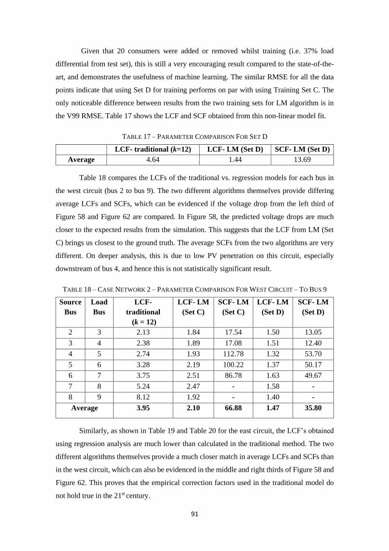
91
Given that 20 consumers were added or removed whilst training (i.e. 37% load
differential from test set), this is still a very encouraging result compared to the state-of-the-
art, and demonstrates the usefulness of machine learning. The similar RMSE for all the data
points indicate that using Set D for training performs on par with using Training Set C. The
only noticeable difference between results from the two training sets for LM algorithm is in
the V99 RMSE. Table 17 shows the LCF and SCF obtained from this non-linear model fit.
TABLE 17 – PARAMETER COMPARISON FOR SET D
LCF- traditional (k=12) LCF- LM (Set D) SCF- LM (Set D)
Average 4.64 1.44 13.69
Table 18 compares the LCFs of the traditional vs. regression models for each bus in
the west circuit (bus 2 to bus 9). The two different algorithms themselves provide differing
average LCFs and SCFs, which can be evidenced if the voltage drop from the left third of
Figure 58 and Figure 62 are compared. In Figure 58, the predicted voltage drops are much
closer to the expected results from the simulation. This suggests that the LCF from LM (Set
C) brings us closest to the ground truth. The average SCFs from the two algorithms are very
different. On deeper analysis, this is due to low PV penetration on this circuit, especially
downstream of bus 4, and hence this is not statistically significant result.
TABLE 18 – CASE NETWORK 2 – PARAMETER COMPARISON FOR WEST CIRCUIT – TO BUS 9
Source
Bus
Load
Bus
LCF-
traditional
(k = 12)
LCF- LM
(Set C)
SCF- LM
(Set C)
LCF- LM
(Set D)
SCF- LM
(Set D)
2 3 2.13 1.84 17.54 1.50 13.05
3 4 2.38 1.89 17.08 1.51 12.40
4 5 2.74 1.93 112.78 1.32 53.70
5 6 3.28 2.19 100.22 1.37 50.17
6 7 3.75 2.51 86.78 1.63 49.67
7 8 5.24 2.47 - 1.58 -
8 9 8.12 1.92 - 1.40 -
Average 3.95 2.10 66.88 1.47 35.80
Similarly, as shown in Table 19 and Table 20 for the east circuit, the LCF’s obtained
using regression analysis are much lower than calculated in the traditional method. The two
different algorithms themselves provide a much closer match in average LCFs and SCFs than
in the west circuit, which can also be evidenced in the middle and right thirds of Figure 58 and
Figure 62. This proves that the empirical correction factors used in the traditional model do
not hold true in the 21st century.

92
TABLE 19 – CASE NETWORK 2 – PARAMETER COMPARISON FOR EAST CIRCUIT – TO BUS 16
Sourc
e Bus
Load
Bus
LCF- traditional
(k = 12)
LCF- LM
(Set C)
SCF- LM
(Set C)
LCF- LM
(Set D)
SCF- LM
(Set D)
2 10 2.05 1.64 9.83 1.50 8.72
10 11 2.13 1.49 8.54 1.34 7.43
11 12 2.65 1.48 5.86 1.07 4.51
12 13 2.96 1.71 4.08 1.53 3.47
13 14 3.75 1.86 4.05 1.80 3.70
14 15 5.24 0.78 - 0.66 -
15 16 12.15 0.93 - 0.61 -
Average 4.42 1.41 6.47 1.21 5.56
TABLE 20 – CASE NETWORK 2 – PARAMETER COMPARISON FOR EAST CIRCUIT – TO BUS 22
Source
Bus
Load
Bus
LCF- traditional
(k = 12)
LCF- LM
(Set C)
SCF- LM
(Set C)
LCF- LM
(Set D)
SCF- LM
(Set D)
2 10 2.05 1.64 9.83 1.50 8.72
10 11 2.13 1.49 8.54 1.34 7.43
11 17 3.28 1.44 23.48 1.72 23.73
17 18 3.49 1.52 17.58 1.86 18.64
18 19 3.75 1.72 12.79 1.88 12.90
19 20 5.24 1.42 16.32 1.19 11.19
20 21 6.29 1.82 -1.52 1.52 -1.07
21 22 12.15 1.57 -4.23 1.82 -2.47
Average 4.80 1.58 10.35 1.60 9.88
The presence of negatives downstream of bus 20 in the SCFs in the table above can
be attributed to the fact that LCF and SCF cannot be independently manipulated. Hence when
there are very few loads at the extremities, we can see negatives in the SCFs. But this does
not lead to vast fluctuations in forecast voltage, and it is not a statistically significant result.
For line 1, tap ratio is predicted as 0.975p.u. using either of the two training sets. This
has not been verified on site but does match the starting voltage specified in the simulator
settings of 224.25V (equal to 0.975 x 230V).
5.2.4. Learning with Training Set D and Testing on Test Set D using CART
When training Set D with CART algorithm, the overall RMSE between predicted and
simulation voltages is 2.15V, which is higher though than the RMSE from LM algorithm
predictions on Test Set D. This may be seen as a strange result given that the RMSE difference

93
in predicted and expected 99-percentiles (voltage rise) for each line voltage is 0.60V and 1-
percentiles (voltage drop) for each line voltage is 1.95V, both an improvement. But this is
another example of how the CART algorithm is overfitting. CART has better performance
when V1 and V99 RMSE are compared only, as evidenced by Figure 62 and Figure 64.
The overall RMSE between predicted and simulation voltages of 2.15V is similar to
RMSE from CART algorithm predictions on Test Set C, as per Table 21. This reconfirms that
using a training set with a different number of consumers to the test set performs on par than
the one where the number of consumers remains the same.
Figure 63 – Expected and predicted results of Set D using CART

94
Figure 64 – Learning with Training Set D and Testing on Test Set D using CART
When comparing the black box and grey box models, as before, it is important to note
that the latter is quicker, avoids overfitting and is more suitable to the needs of
parametrisation.
TABLE 21 – COMPARISON OF RMSE BETWEEEN BLACK BOX AND GREY BOX METHODS (V)
Algorithm
/ Test Set
RMSE between all
prediction and
simulation voltages
RMSE between
predicted V99 and
simulation V99
RMSE between
predicted V1 and
simulation V1
LM / Set C 1.87 1.40 2.82
CART / Set C 2.20 0.17 0.90
LM / Set D 1.90 2.69 2.62
CART / Set D 2.15 0.60 1.95
5.3. Summary and Discussion
In this chapter, we have presented our results and a discussion around our findings.
We have looked at 2 different case networks in this chapter to analyse our methodology.
We begin with simulating the Case Network 1, a model of a real-world distribution
network. The 21 bus voltages for each time instance for a year are taken. We verify our 2
machine learning algorithms are performing as expected by training and testing on the same
data set (first half of the year) and getting a very close match between predictions and the
data set. We then test the non-linear and decision tree models on the voltage data of the second
half of the year. In this manner, we have demonstrated that given new household load data (P
and Q), voltages can be forecast for a given network topology using both learning methods.
For sensitivity, we create a forward-looking scenario with high PV penetration to see
the effects this has on voltage rise predictions as well as new LCF and SCF parameters. We

95
repeat the methodology of training and testing on different halves of the year for Case
Network 2 using the two learning algorithms. The overall RMSEs did rise since large swings
in voltage (day-time and night-time) make it difficult to predict. But both the learning
methods performed better than the voltage drop from the traditional method. Given that the
traditional method does not produce a voltage rise, this is seen as an important success. The
decision tree model is suitable for the needs of finding voltage headroom, but consistently
performs worse overall than the non-linear model fit as seen in the first column in Table 21.
We then use these algorithms for training on voltage data from networks of 20 more
and 20 fewer households than both Case Network 1 and Case Network 2. Both algorithms
are able to predict voltages for the whole year from the relevant Case Network (with the
original number of customers) with small RMSEs.
When comparing the grey box and black box solutions, the former is quicker and
avoids overfitting. It is also more suited for our needs of obtaining trained parameters for
diversity, unbalance and transformer turns ratio (tap). The black box model performs better
in predicting the upper and lower bounds of the voltage range for every bus. The overall
RMSE for each time instance, though, is higher than grey box, which may be its biggest
shortcoming depending upon the application.

96
CHAPTER 6 – CONCLUSIONS
6.1. Summary of Thesis
In Chapter 1, we see that Governments around the world are increasingly pledging
for carbon emission reductions. The emphasis is on using clean technologies in the power
generation sector. At a policy level in Australia, for example, there is an emphasis to provide
energy sustainably, securely, and cheaply; consistent with Australia’s obligations in the
international climate change mitigation effort. Australia is poised to see a dramatic shift away
from its high reliance on coal; to solar and wind-power, and a highly decentralised structure
in the form of rooftop PV and behind-the-meter batteries. Appropriate electricity market
designs and new energy policies will see solar rooftop penetration in households increase to
a large-scale over the next few years. An example of this is the 2019 Victorian Solar Homes
Program [5] which provides 50% subsidies towards rooftop PV and embedded storage. This
will encourage accelerated rates of rooftop PV adoption, making it a viable method to reduce
household electricity bills. But this will lead to many technical issues for DNOs and network
planning engineers such as:
• Voltage fluctuations caused by intermittent PV generation (cloud passage);
• Voltage regulation (voltage rise);
• Significant reverse power flow resulting in overloading of upstream network assets;
and
• System stability.
In this thesis, we focus on voltage regulation issues and voltage estimation techniques
being used when new prosumer applications are received. In the local electricity supply

97
industry, existing feeder voltage estimation methods are based on empirical or probabilistic
methods that can be traced back to 1940’s and do not incorporate two-way power-flow
brought about by PV units. Given the relatively predictable operating regime and low level
of LV monitoring, there has not been much research and innovation done to create new
voltage estimation techniques. Currently used techniques are based on conservative
assumptions or rely on the design engineer’s local area knowledge of the network to source
the correct inputs. Some commercially available software such as LVDesign and LVDrop
provide better results but provide voltages at only one point of time instead of a time series.
Techniques mentioned in literature have been probabilistic, empirical, statistical or “bottom-
up” as shown in Chapter 2. There have been no attempts to predict voltages based on future
connections that are not statistical probabilistic, or purely deterministic. A balanced approach
is required; that helps voltage regulation calculations to be done quickly and accurately.
In this Master Dissertation, a modern approach for calculating voltage drop and
voltage rise in a real-world LV feeder is shown using standard machine learning tools.
Various network components are first modelled in Chapter 3 and technical details are
presented on the 400V distribution network in Australia. There are identified 5 upstream
network components that lead to voltage regulation that an end-customer sees at the point of
connection. These hence affect headroom available to connect either PV or load at any given
residential premises. Whilst 4 of these components are to a certain degree estimable, voltage
regulation within the LV feeder mains is dependent on various factors which makes it difficult
to ‘control’. Given power consumption data for each household is available through interval
meters, there has been no previous attempt made to revisit voltage estimation methodologies
to answer the question: “how much further voltage drop or rise is a new connection expected
to cause on the network?”
Chapter 4 details the machine learning methodology proposed. Household interval
metering data (for load and generation) and the topology of a network are provided by the
local utility which we use to form a model of Case Network 1 in OpenDSS. A load-flow
simulation of this real-world network is carried out based on conductor data from the
manufacturer; and span lengths, transformer size, transformer impedance and phase
information for each customer as found on site. We obtain voltages at each node or pole, as
well as real power consumed, real power generated and apparent power consumed
downstream of each node. Using this data, test and training sets are created from different
halves of the year. Case Network 2 is prepared using the same topology, but with much higher
PV penetration. The process for creating training and test data sets is repeated.

98
Next the traditional relationship between voltages, load and circuit impedance for
calculating voltage drop is renewed to include a solar PV correction factor to allow for voltage
rise calculations as well. A non-linear regression model is then modelled on the modified
relationship. Parameters for the regression model are identified as load and solar correction
factors. These account for demand diversity and phase unbalance in household loads and
rooftop PV units. For bus 1, a third parameter is also introduced in the aforementioned
relationship so that the starting voltage of bus 1 can be calibrated with upstream voltage
regulation in the MV network. These parameters are trained and the results of the regression
model predictions are shown in Chapter 5. This non-linear regression model is shown to
accurately and quickly predict voltage variations in the network. Error on the LV network
is 1.22V across 21 nodes and 99,645 time-intervals, when training and testing on different
halves of the year, even though consumption patterns and solar irradiation patterns change
due to different seasons in the test data run. When training and testing on networks with
different number of connections, error on the network is only 1.32V. The methodology
hence holds up when tested on a network with a different number of residences than on which
it was trained. These results are significant given that 20 consumers were added or removed
on a case network of only 54 households. This methodology proves that we can use regression
to learn what makes the voltage profile behave a certain way from the training data. Using
those learned characteristics, the algorithm then produces the new voltage profile based on
new input data i.e. is able to predict the voltage. This is the basis of our time-series regression
solution. Next, we compare the LCF obtained from our grey box model to those used in
traditional volt-drop estimation techniques. In Case Network 1, we find that the traditional
method LCF indicates much higher (around 2.5 times) allowance for phase unbalance
and diversified demand as obtained from our regression model. Empirical methods used in
the traditional model hence do not necessarily hold true in the 21st century. SCF created for
PVs in our regression model for each bus provide a higher order of flexibility. This,
undoubtedly, enables predictions of bus voltages from machine learning to be far superior to
the traditional method.
This methodology is repeated by using a different learning method i.e. CART. Even
though the results from this decision tree model for determining the voltage headroom
available are superior, there are concerns regarding acceptance of this black box model in
industry as it presents no actionable parameters.
Case Network 2 with high PV penetration is then tested using the same workflow as
Case Network 1. The results from both learning methods are still accurate, with or without

99
additional consumers on the network that the training data did not have. This proves that the
learned structure can also be applied beyond the training data. Furthermore, the predicted tap
position is shown to exactly match the one modelled in the simulation, for both case networks.
When comparing black box to grey box methods, both provide highly accurate
results. We hence see no reason to improve the grey box methodology, as it additionally
provides trained parameters for each span. The classical black box model is shown to be prone
to overfitting and is slower to train as well. Better black box models may be used, but this is
beyond the scope of our work.
6.2. Summary of Contributions
Digital technologies are rapidly transforming industries in Australia and around the
world. Utilities too should use technology-driven innovation to generate efficiencies across
their enterprises, improve customer satisfaction, improve planning practices and understand
LV feeder voltages. It is clear that the obligation to manage power quality will turn into
obligation to enable or manage solar exports. But note that there is limited appetite for
network investment. To support this, we have demonstrated that data ingestion, forecasting
and analysis can be deployed in practical terms. Although on the surface, this research and
its conclusions may seem specific to the Victorian (or Australian) context, the insights
obtained may inform decision-making elsewhere. The methodology is location independent,
and is well suited for the modern LV grid where interval metering data is readily available.
On the other hand, there may be some professionals who see this work as risky as it
may be usurped by a ‘Network of the Future’. This is characterised as having active LV
network management including better topological and network connectivity information (i.e.
supply point associations between meter and upstream transformer). This is foreseen to allow
data collection, aggregation and real-time or automated voltage investigations. But such a
scenario may be a decade or two ahead of us. Meanwhile, regulating bodies and utilities, in
the interest of avoiding PV export limits, have a very imminent need to predict LV feeder
voltages with an ever-increasing rooftop solar penetration.
The contributions of this thesis can be summarised below:
One of the first main contributions of this work is the literature survey done on all the
differing methods in academia of calculating voltage drop and rise in LV feeders. This

100
extensive work should prove useful to other network planners and researchers alike as it also
covers methods used in a wide variety of local and international utilities.
In this Dissertation, a new approach to compute voltage drop in an LV feeder is
presented. The proposed method also calculates accurate voltage rise in the LV feeder in-case
of bi-directional power flow due to PV. This is a vital contribution since this will help further
reduce barriers to PV adoption such as expensive augmentation works that are passed on to
the customers, either upfront or through lowering of network prices over time.
Two machine learning methods used in this research have different advantages and
may be used by network planners for different applications. The decision tree model performs
very well when predicting the V1 and V99 at each node and hence can calculate the
magnitude of any voltage violations. This is useful for predicting available voltage headroom
once a new load or PV connection is made. Comparatively, the non-linear regression model
is shown to be slightly less accurate for predicting available headroom, but we see no reason
to pursue alternate techniques such as deep learning or Artificial Neural Networks. The
strength of the non-linear regression lies in predicting voltages at every half-hour interval
over a year. This is more useful for applications where the total number or the frequency of
voltage violations with a proposed connection is of importance. Such an application could be
used for proving to the regulator, for example, that the number of violations does not exceed
a given amount in a year. Although DNOs do not face harsh fiscal penalties from regulating
authorities for voltage excursions, there is a clear benefit for the DNO to prioritise feeders
that have high number of voltage excursions; as they can indicate other issues such as high
phase imbalance, high peak load, incorrect tap setting or a long circuit. This method can hence
help in prioritising different constrained LV feeders as the higher the number of predicted
excursions, the higher the risk of customer complaints and/ or liability. The strength of the
non-linear regression over the decision tree method also lies in creating a grey box model,
which can be easily understood and implemented in the industry by retrofitting into existing
methods such as spreadsheets modelled on Equation (16). Not using traditionally exaggerated
empirical or probabilistic allowances for diversity or unbalance will facilitate more informed
technical assessments and better utilisation of assets. The cost of performing any analysis will
be a miniscule fraction of potential cost involved in network upgrades. Hence, our work caters
to the practical realities and best practices of system planning.

101
This thesis shows that forecasts made with machine learning are quite reliable and
perform well with small MSE compared to simulation results. The proposed methodology
incorporates half-hour interval metering data now more and more readily available in the
developed world. An ideal smart grid system should be built on measuring information at the
most appropriate time intervals such that the data can be refined down to information useable
for a wide range of cases with minimal overheads. And we show that half-hour interval data
is appropriate for the proposed application. Not choosing to use 10-second or 5-minute data
from smart meters helps us avoid the complications of using highly granular data which have
the potential to create data management and data storage constraints. This work demonstrates
a practical use of the consumption data accessible to utilities, which is not being analysed for
the purpose of estimating future voltages.
6.3. Future Works
Some added features to the methodology will lead to an improved final solution. For
example, predicted voltages shown here are steady-state values and don’t take into
consideration the intermittent fluctuations in voltages due to cloud cover. This could be
explored in the future.
This research acts as a guide for technical planning of residential LV networks and
compliance with voltage limit regulations. Further analysis can be done by introducing short-
term forecast capability (using weather correction for upcoming summer for example); or
long-term (localised economic growth indices or population/ load growth indices). Network
planners or researchers can also associate a monetary risk with the voltage excursions
predicted through the methodology presented here, forecast for different weather conditions
(50% POE or 10% POE days). Depending on the overall voltage excursion duration and
voltage excursion frequency per customer, engineers can take interest in financial modelling
of augmentation works vs. the monetary risk of voltage violations. This will allow engineers
to perform cost-benefit analysis and perform project prioritisation. This could even help the
poles-and-wires companies to pivot towards a different business model. For example, where
incentivising new households connecting onto the grid with a PV-battery combination
presents a lower risk of voltage violations and an overall cheaper solution compared to
augmentation works.
The methodology can also be used to study the effect of emerging technologies like

102
EVs and batteries on voltage regulation. Ultimately, this will allow distribution networks to
evolve with the changing mix of renewables and distributed energy resources. Researchers
will be able to use the same methodology to study those disruptors in detail by overlaying
them onto the network. Testing of different voltage management strategies can be performed
which can then be validated in a lab. Inverter testing in the field for comparison will be still
better. Forecasting voltages can be hugely beneficial to Virtual Power Plants with smart
control algorithms set-up. In cases of low voltages forecast, such algorithms could request
batteries to supply power to the grid to support local voltages. And in cases of high voltages,
the algorithms could request EV charging, thus increasing load and reducing voltages on the
network. There is no doubt that this will be valuable work, especially if an Application
Programming Interface (API) can be created for publishing operating envelopes (for
individual and aggregated distributed energy resources), which will help demonstrate an
orchestration-based approach used by DER providers and aggregators. An online map created
using this API will also help empower and educate prosumers.
Further work can be done to use machine learning to predict existing circuit
impedances, given circuit lengths. Comparing the calculated impedance with standard
conductor impedance database will help determine the type of existing LV conductors on the
network which is highly beneficial for any DNO due to scarce conductor data in their GIS.
Machine learning can also be used to predict distribution transformer tap position
using the existing AMI voltage data and upstream SCADA (Supervisory Control and Data
Acquisition) data of MV levels on the primary side. This will be a vital achievement for any
DNO as it will reduce operating expenditure involved with sending out linesmen and
technicians on site to record tap settings.
Studies on static voltage stability, power losses in the network and short-circuit and
fault level in the presence of growing number of PVs can all be included in future research
using the same methodology presented here.

103
REFERENCES:
[1] A. B. Gupta, T. Alpcan, and A. B. Morton, "Predicting Voltage Variations in Low
Voltage Networks with Prosumers," in IEEE PES Asia-Pacific Power and Energy
Engineering Conference (APPEEC), 2018, pp. 183-188.
[2] United Nations Framework Convention on Climate Change. (2015). Paris Agreement.
Available:
https://unfccc.int/files/meetings/paris_nov_2015/application/pdf/paris_agreement_engli
sh_.pdf
[3] S. Henbest. (04 August 2019). Bloomberg New Energy Outlook. Available:
https://bnef.turtl.co/story/neo2019
[4] International Energy Agency. (2017). 978-92-64-28230-8, World Energy Outlook.
Available: https://www.iea.org/media/weowebsite/2017/Chap1_WEO2017.pdf
[5] "Victoria's Rooftop Solar Revolution Kicks Off Today," Victorian Government,
Melbourne, Australia, 1 July 2019, Available: https://www.premier.vic.gov.au/wp-
content/uploads/2019/07/190701-Victoria%E2%80%99s-Rooftop-Solar-Revolution-
Kicks-Off-Today.pdf, Accessed on: 04 August 2019.
[6] Australian Energy Council. (2018). Solar Report Quarter 2. Available:
https://www.energycouncil.com.au/media/13264/aec-solar-report_-q2-2018.pdf
[7] "Solar Map, funded by the Australian Renewable Energy Agency," Australian PV
Institute (APVI), Sydney, Australia, 2018, Available: http://pv-map.apvi.org.au/,
Accessed on: 18 August 2018.
[8] P. Kilby, "Voltage management on distribution networks with high PV penetrations," in
"Power, Energy and Clean Technologies Seminar," Queensland University of
Technology (QUT), Brisbane, 03 May 2019, Available:
https://cloudstor.aarnet.edu.au/plus/s/mirvqhr59avqc7G#pdfviewer, Accessed on: 04
August 2019.

104
[9] A. B. Morton, "Potential of and limitations to Distributed management of LV and MV
feeder voltage profiles with high penetration of embedded generation and storage," in
CIGRE 2018 Session, Paris, France, no. 47.
[10] D. Stolper, J. Hoye, and B. Wegener, "Community attitudes toward Solar," Newgate
Research for South Australia Power Networks (SAPN), Adelaide, 2018, Available:
https://www.talkingpower.com.au/43062/documents/100573/download, Accessed on:
04 August 2019.
[11] "Power of choice implementation program industry accreditation and registration plan,"
Australian Energy Market Operator, 28 April 2017, Available:
https://www.aemo.com.au/-/media/Files/Electricity/NEM/Power-of-
Choice/B2B/2017/AEMO-POC-Industry-Accrediation-and-Registration-Plan-v10.pdf,
Accessed on: 04 August 2019.
[12] "Global Market Outlook For Solar Power 2018 - 2022," Solar Power Europe, Brussels,
2018, Available: http://www.solarpowereurope.org/wp-
content/uploads/2018/09/Global-Market-Outlook-2018-2022.pdf, Accessed on: 04
August 2019.
[13] R. Tsao, "TrendForce Forecasts Global Solar Market to Reach Over 106GW in 2018
Due to Strong Momentum from China and Rebounding Demand in Europe," ed:
TrendForce, 2018.
[14] International Energy Agency. (2018). IEA PVPS T1-33:2018, Snapshot of global
photovoltaic markets. Available: http://www.iea-
pvps.org/fileadmin/dam/public/report/statistics/IEA-PVPS_-
_A_Snapshot_of_Global_PV_-_1992-2017.pdf
[15] M. A. Hayat, F. Shahnia, and A. Arefi, "Comparison of the electricity tariffs and bills
across the zones of Australian power distribution companies," in Australasian
Universities Power Engineering Conference (AUPEC), 2016, pp. 1-6: IEEE.
[16] Grid connection of energy systems via inverters - Installation requirements, 2016.
[17] G. Walker, "Customer distributed generation sources and their integration to the grid,"
in "Adapting to Meet Customer Expectations," Queensland University of Technology
(QUT), Brisbane, 23 Feb 2016, Available:
https://eeaust.com.au/images/stories/virtuemart/category/API_Customer_DE_Grid%20I
ntegration_20160223%20Geoff.pdf, Accessed on: 04 August 2019.
[18] "Unleashing the Potential of Solar & Storage," SolarPower Europe, Brussels, 2018,
Available: http://www.solarpowereurope.org/wp-content/uploads/2018/09/Mini-report-
FINAL.pdf, Accessed on: 04 August 2019.
[19] "Clean Energy Australia Report 2018," Clean Energy Council, Melbourne, 2018,
Available: https://assets.cleanenergycouncil.org.au/documents/resources/reports/clean-
energy-australia/clean-energy-australia-report-2018.pdf, Accessed on: 04 August 2019.
[20] K. Petrou et al., "Limitations of Residential Storage in PV-Rich Distribution Networks:
An Australian Case Study," in 2018 IEEE Power & Energy Society General Meeting
(PESGM), 2018, pp. 1-5.
[21] A. Chidurala, "High penetration of PV systems in low voltage distribution networks:
Investigation of power quality challenges and mitigation," Doctor of Philosophy,

105
School of Information Technology and Electrical Engineering, The University of
Queensland, Brisbane, 2016.
[22] G. S. Ivanovich, "Modern distribution planning and application to development of
electricity infrastructure," M.S. Thesis, Dept. Eng. and Surveying, Univ. of Southern
Queensland, Toowoomba, 2010.
[23] Y. Zhao, Y. An, and Q. Ai, "Research on size and location of distributed generation
with vulnerable node identification in the active distribution network," IET Generation,
Transmission & Distribution, vol. 8, no. 11, pp. 1801-1809, 2014.
[24] S. Abapour, K. Zare, and B. Mohammadi-ivatloo, "Evaluation of technical risks in
distribution network along with distributed generation based on active management,"
IET Generation, Transmission & Distribution, vol. 8, no. 4, pp. 609-618, 2014.
[25] Electricity Services Commission. (2018). Electricity Distribution Code. Available:
https://www.esc.vic.gov.au/sites/default/files/documents/Electricity-Distribution-Code-
version-9A-August-2018_0.pdf
[26] R. Tonkoski, D. Turcotte, and T. H. El-Fouly, "Impact of high PV penetration on
voltage profiles in residential neighborhoods," IEEE Transactions on Sustainable
Energy, vol. 3, no. 3, pp. 518-527, 2012.
[27] A. Thomas, "Calculating Voltage Rise," Ergon Energy, Maryborough, Australia, 2011.
[28] S. Lewis, "Analysis and management of the impacts of a high penetration of
photovoltaic systems in an electricity distribution network," in Innovative Smart Grid
Technologies Asia (ISGT), 2011 IEEE PES, 2011, pp. 1-7: IEEE.
[29] M. J. Alam, K. Muttaqi, and D. Sutanto, "A three-phase power flow approach for
integrated 3-wire MV and 4-wire multigrounded LV networks with rooftop solar PV,"
IEEE Transactions on Power Systems, vol. 28, no. 2, pp. 1728-1737, 2013.
[30] M. Thomson and D. G. Infield, "Network Power-Flow Analysis for a High Penetration
of Distributed Generation," IEEE Transactions on Power Systems, vol. 22, no. 3, pp.
1157-1162, 2007.
[31] "AEMC Reliabillity Panel, 2017 Annual Market Performance Review, Final Report,"
Australian Energy Market Commission, Sydney, Australia, 20 Mar 2018, Available:
https://www.aemc.gov.au/sites/default/files/2018-03/Final%20report.pdf, Accessed on:
04 August 2019.
[32] "Electromagnetic compatibility (EMC) - Limits - Steady state voltage limits in public
electricity systems," in "AS/NZS 61000.3.100," Council of Standards Australia,
Sydney, Australia, 23 December 2011.
[33] N. K. Roy, H. R. Pota, and M. A. Mahmud, "DG integration issues in unbalanced multi-
phase distribution networks," in 2016 Australasian Universities Power Engineering
Conference (AUPEC), 2016, pp. 1-5.
[34] S. Elphick and D. Robinson, "Impact of Distributed Generation on Power Quality,"
Australian Power Quality and Reliability Centre/ Sustainable Buildings Research
Centre, Wollongong, 2018.

106
[35] P. Gnacinski, "Windings Temperature and Loss of Life of an Induction Machine Under
Voltage Unbalance Combined With Over- or Undervoltages," IEEE Transactions on
Energy Conversion, vol. 23, no. 2, pp. 363-371, 2008.
[36] G. M. Masters, Renewable and Efficient Electric Power Systems. Wiley, 2013.
[37] "Electricity forecasting insights for the national electricity market," Australian Energy
Market Operator, 30 June 2017, Available: https://www.aemo.com.au/-
/media/Files/Electricity/NEM/Planning_and_Forecasting/Demand-Forecasts/EFI/2017-
Electricity-Forecasting-Insights.pdf, Accessed on: 04 August 2019.
[38] "Distribution System Planning (Asset Management Plan 1.1.01)," in "Distribution
System Planning Report," South Australia Power Networks (SAPN), Adelaide, 27 Oct
2014, Available: https://www.aer.gov.au/system/files/SAPN%20-
%207.4%20PUBLIC%20-
%20SAPN%20Distribution%20System%20Planning%20Report%20%28AMP%201.1.
01%29.pdf, Accessed on: 04 August 2019.
[39] C. Bary, "Coincidence-Factor Relationships of Electric-Service-Load Characteristics,"
Trans. AIEE, vol. 64, no. 9, pp. 623-628, September 1945.
[40] P. Caramia, G. Carpinelli, P. Varilone, and P. Verde, "Probabilistic three-phase load
flow," International Journal of Electrical Power & Energy Systems, vol. 21, no. 1, pp.
55-69, January 1999.
[41] J. Boggis, "Diversity, Bias and Balance," Distribution of Electricity, pp. 357-362, July
1953.
[42] B. Axelsson and C. G. Strand, "Computer as Controller and Surveyor of Electrical
Distribution Systems for 20, 10, 6 and 0.4 kV," in 2nd International Conference on
Electricity Distribution, Liege, Belgium, 1975, vol. 8, pp. 210-220.
[43] A. Capasso, W. Grattieri, R. Lamedica, and A. Prudenzi, "A bottom-up approach to
residential load modeling," IEEE Transactions on Power Systems, vol. 9, no. 2, pp. 957-
964, 1994.
[44] D. McQueen, M. Mcqueen, P. Hyland, and S. Watson, "Simulation of power quality in
residential electricity networks," in Power Quality, 2015.
[45] K. A. Gosden, "A statistical method for analysing L.V. distribution networks,"
presented at the Annual Conference of the Electricity Supply Eng. Association of NSW,
Sydney, New South Wales, August 13-16, 1990.
[46] R. Herman and C. T. Gaunt, "A Practical Probabilistic Design Procedure for LV
Residential Distribution Systems," IEEE Transactions on Power Delivery, vol. 23, no.
4, pp. 2247-2254, 2008.
[47] A. Soroudi, M. Aien, and M. Ehsan, "A Probabilistic Modeling of Photo Voltaic
Modules and Wind Power Generation Impact on Distribution Networks," IEEE Systems
Journal, vol. 6, no. 2, pp. 254-259, 2012.
[48] J. Dickert and P. Schegner, "Residential load models for network planning purposes," in
Modern Electric Power Systems (MEPS), 2010 Proceedings of the International
Symposium, 2010, pp. 1-6.

107
[49] E. Namanya, "Voltage Calculation on Low Voltage Feeders with Distributed
Generation," Master of Science in Engineering, Department of Electrical Engineering,
University of Cape Town, Cape Town, 2014.
[50] Y. M. Atwa, E. F. El-Saadany, M. M. A. Salama, and R. Seethapathy, "Optimal
Renewable Resources Mix for Distribution System Energy Loss Minimization," IEEE
Transactions on Power Systems, vol. 25, no. 1, pp. 360-370, 2010.
[51] Y. Li, "Statistical and probabilistic models for smart electricity distribution networks,"
PhD, Department of Electrical and Computer Engineering, Curtin University, Perth,
2013.
[52] P. Boait, V. Advani, and R. Gammon, "Estimation of demand diversity and daily
demand profile for off-grid electrification in developing countries," Energy for
Sustainable Development, vol. 29, pp. 135-141, 2015.
[53] S. Eftekharnejad, V. Vittal, G. T. Heydt, B. Keel, and J. Loehr, "Impact of increased
penetration of photovoltaic generation on power systems," IEEE transactions on power
systems, vol. 28, no. 2, pp. 893-901, 2013.
[54] M. E. Baran and F. F. Wu, "Network reconfiguration in distribution systems for loss
reduction and load balancing," IEEE Transactions on Power delivery, vol. 4, no. 2, pp.
1401-1407, 1989.
[55] M. E. Baran and F. F. Wu, "Optimal sizing of capacitors placed on a radial distribution
system," IEEE Transactions on Power Delivery, vol. 4, no. 1, pp. 735-743, 1989.
[56] L. Wang, D. H. Liang, A. F. Crossland, P. C. Taylor, D. Jones, and N. S. Wade,
"Coordination of multiple energy storage units in a low-voltage distribution network,"
IEEE Transactions on Smart Grid, vol. 6, no. 6, pp. 2906-2918, 2015.
[57] D. H. McQueen, P. R. Hyland, and S. J. Watson, "Monte Carlo simulation of residential
electricity demand for forecasting maximum demand on distribution networks," IEEE
Transactions on power systems, vol. 19, no. 3, pp. 1685-1689, 2004.
[58] J. Dickert, G. Seth, and P. Schegner, "Comparison of design concepts for AC low
voltage distribution networks," in PES General Meeting| Conference & Exposition,
2014 IEEE, 2014, pp. 1-5: IEEE.
[59] D. L. Nickel and H. R. Braunstein, "Distribution Transformer Loss Evaluation: II -
Load Characteristics and System Cost Parameters," IEEE Transactions on Power
Apparatus and Systems, vol. PAS-100, no. 2, pp. 798-811, 1981.
[60] S. Rusck, "The simultaneous demand in distribution network supplying domestic
consumers," ASEA Journal, vol. 10, pp. 59-61, 1956.
[61] F. Provoost, "Intelligent distribution network design," Ph.D. dissertation, Elect. Eng.,
Technische Universiteit Eindhoven, 2009.
[62] H. L. Willis, Power distribution planning reference book, 2nd ed. New York: M.
Dekker, 2004, pp. xix, 1217 p. [Online]. Available:
http://marc.crcnetbase.com.ezp.lib.unimelb.edu.au/isbn/9781420030310 Connect to
ebook (University of Melbourne only).

108
[63] A. Baitch, "Voltage Control for Distribution Networks and the 230V/400V Standard,"
presented at the Annual Conference of the Electric Energy Society of Australia,
Canberra, Australian Capital Territory, 4th August, 2000.
[64] A. Navarro, L. F. Ochoa, and P. Mancarella, "Learning from residential load data:
Impacts on LV network planning and operation," in 2012 Sixth IEEE/PES Transmission
and Distribution: Latin America Conference and Exposition (T&D-LA), 2012, pp. 1-8.
[65] Electricity Council, "Report on the Design of Medium Voltage Underground Networks
for New Housing Estates," in Area Board Chief Engineers' (ACE) Report No. 13, U.K.,
1966.
[66] Central Electricity Authority and Area Boards, "Report on the Design of Underground
Distribution Systems for New Housing Estates," U.K., June 1954.
[67] M. Davies and R. G. Paterson, "Phase unbalance in low-voltage distribution systems,"
Proceedings of the IEE - Part A: Power Engineering, vol. 109, no. 48, pp. 535-541,
1962.
[68] Energy Networks Association, "Report on the design of Low Voltage underground
networks for new housing," presented at the Area Boards Chief Engineers' (ACE)
Report No. 105, London, U.K., 1986.
[69] J. Vo, "LV Design Frequently Asked Questions," Western Power, Perth, 31 July 2007,
Available: https://westernpower.com.au/media/1521/lv-design-faqs.pdf, Accessed on:
04 August 2019.
[70] N. Gourley, "Framework for design & planning of LV housing developments, including
U/G networks and associated HV/ LV S/S," S. P. Energy Networks, Scotland,
U.K.,May 2013.
[71] M. Smith, "Specification for Planning & Design of Greenfield Low Voltage Housing
Estates," Scottish and Southern Energy, Scotland, U.K., 2003.
[72] Energy Networks Association, "Report on the Statistical method for calculating
demands and voltage regulations on LV radial distribution systems," presented at the
Area Boards Chief Engineers' (ACE) Report No. 49, London, U.K., 1981.
[73] "Design and construction standard for URDs," in "Network Standard," Ausgrid,
Sydney, 08 April 2019, Available: https://www.ausgrid.com.au/-
/media/Documents/Technical-Documentation/NS/NS110.pdf, Accessed on: 04 August
2019.
[74] "Method of calculating voltage drop in low voltage mains," in "Mains Design
Instruction," Endeavour Energy, Huntingwood, Australia, 22 October 2014, Available:
http://www.endeavourenergy.com.au/wps/wcm/connect/2e9da97d-4aad-4191-8ae0-
33487f9679d8/MDI+0030.pdf?MOD=AJPERES, Accessed on: 04 August 2019.
[75] T. Haggis, "Network Design Manual," E.ON Central Networks, U.K., 2006, Available:
https://www.yumpu.com/en/document/read/8953808/network-design-manual-eon-uk,
Accessed on: 04 August 2019.
[76] P. V. Rhyn, "Probablistic low voltage distribution network design for aggregated light
industrial loads," Ph.D. dissertation, Faculty of Eng., Univ. of Johannesburg, Gauteng,
2011.

109
[77] C. Barteczko-Hibbert, "After Diversity Maximum Demand Report," in "Customer-Led
Network Revolution," Durham University, U.K., 2015, Available:
http://www.networkrevolution.co.uk/wp-content/uploads/2015/02/After-Diversity-
Maximum-Demand-Insight-Report.pdf.
[78] S. Mingyang, I. Konstantelos, and G. Strbac, "Analysis of diversified residential
demand in London using smart meter and demographic data," in 2016 IEEE Power and
Energy Society General Meeting (PESGM), 2016, pp. 1-5.
[79] R. Herman, J. Maritz, and J. Enslin, "The analysis of voltage regulation in residential
distribution networks using the beta distribution model," Electric power systems
research, vol. 29, no. 3, pp. 213-216, 1994.
[80] R. Herman and J. J. Kritzinger, "The statistical description of grouped domestic
electrical load currents," Electric Power Systems Research, vol. 27, no. 1, pp. 43-48,
1993.
[81] H. C. Kadada, "Designing low voltage feeders to meet quality of supply specifications
for voltage variations," University of Cape Town, 2012.
[82] V. Garrone, "Distribution Voltage Management and the Accommodation of PV," in
"Meeting the Challenge of Change," UQ (The University of Queensland) Solar / Global
Change Institute, Sunshine Coast, 29 Feb 2016, Available:
http://eeaust.com.au/images/stories/virtuemart/category/api-2016-summer-school---
voltage-management-&-pv---garrone-v1.2-4-3.ppsx, Accessed on: 04 August 2019.
[83] "Power Quality Strategic Plan 2015-2020," Energex Limited, Brisbane 25/09/2014,
issue 1.
[84] "Power Quality Augex Forecast 2015/16 - 2019/20," Energex Limited, Brisbane
23/06/2015, issue 1.
[85] J. D. Watson, N. R. Watson, D. Santos-Martin, A. R. Wood, S. Lemon, and A. J. Miller,
"Impact of solar photovoltaics on the low-voltage distribution network in New
Zealand," IET Generation, Transmission & Distribution, vol. 10, no. 1, pp. 1-9, 2016.
[86] A. Canova, L. Giaccone, F. Spertino, and M. Tartaglia, "Electrical impact of
photovoltaic plant in distributed network," IEEE Transactions on industry applications,
vol. 45, no. 1, pp. 341-347, 2009.
[87] "Advice on electricity regulation timely electricity connections," Essential Services
Commission, Melbourne, 07 Sep 2018, Available:
https://www.esc.vic.gov.au/sites/default/files/documents/advice-on-electricity-
regulation-timely-electricity-connections-20180907.pdf, Accessed on: 04 August 2019.
[88] T. A. Short, Distribution reliability and power quality, Boca Raton.: CRC/Taylor &
Francis, 2006, p. 268 p. [Online]. Available:
http://marc.crcnetbase.com.ezp.lib.unimelb.edu.au/isbn/9781420036480 Connect to
ebook (University of Melbourne only).
[89] E. Lakervi, E. J. Holmes, and Institution of Electrical Engineers., Electricity distribution
network design, 2nd ed. (IEE power series, no. 21). London: P. Peregrinus on behalf of
the Institution of Electrical Engineers, 1995, pp. ix, 325 p.

110
[90] N. Browne, "Voltage Management with Distributed Generation," Endeavour Energy,
Wollongong, 2018.
[91] "Victorian Electricity Supply Industry (VESI) Fieldworkers Handbook," Melbourne,
2008, Available:
http://www.vesi.com.au/files/WorkPractices/Fieldworker_Handbook/VESI_FIELDWO
RKERS_MANUAL.PDF, Accessed on: 04 August 2019.
[92] J. D. Glover, M. S. Sarma, and T. J. Overbye, Power system analysis and design.
Wadsworth/Thomson Learning, 2002.
[93] M. Reta-Hernández, "Transmission line parameters," ed: Boca Raton, FL, USA: CRC
Press, 2012.
[94] R. C. Dugan and T. E. McDermott, "An open source platform for collaborating on smart
grid research," in 2011 IEEE Power and Energy Society General Meeting, 2011, pp. 1-
7.
[95] (04 August 2019). Nexans Olex Aerial Catalogue. Available:
https://olex.com.au/Australasia/2012/OLC12641_AerialCat.pdf
[96] T. Longstaff, "Addressing impacts through optimisation," in "Positioning the network to
maximise DER uptake," Ausnet Services, Melbourne, Australia, 5 June 2018,
Available: https://www.ausnetservices.com.au/-/media/Files/AusNet/About-
Us/Determining-Revenues/Distribution-Network/Customer-Forum/Weeks-3-and-
4/Distributed-Energy-Resources-integration.ashx?la=en, Accessed on: 04 August 2019.
[97] P. Järventausta et al., "Using advanced AMR system in low voltage distribution
network management," in 19th International Conference on Electricity Distribution,
2007.
[98] A. Navarro, L. Ochoa, R. Shaw, and D. Randles, "Reconstruction of low voltage
networks: From GIS data To power flow models," in 23rd International Conference on
Electricity Distribution CIRED 2015, 2015, pp. 1-5.
[99] R. C. Dugan and D. Montenegro, "Reference Guide The Open Distribution System
Simulator (OpenDSS) " Electric Power Research Institute, Inc.2019, Available:
ftp://197.155.77.3/sourceforge/e/el/electricdss/OpenDSS/OpenDSSManual.pdf,
Accessed on: 04 August 2019.
[100] A. Crossland, "Application of stochastic and evolutionary methods to plan for the
installation of energy storage in voltage constrained LV networks," Durham University,
2014.
[101] F. C. Pereira and S. S. Borysov, "Chapter 2 - Machine Learning Fundamentals," in
Mobility Patterns, Big Data and Transport Analytics, C. Antoniou, L. Dimitriou, and F.
Pereira, Eds.: Elsevier, 2019, pp. 9-29.
[102] J. Biamonte, P. Wittek, N. Pancotti, P. Rebentrost, N. Wiebe, and S. Lloyd, "Quantum
machine learning," Nature, vol. 549, p. 195, 09/13/online 2017.
[103] MATLAB. (2018-05-12). fitnlm: Fit nonlinear regression model. Available:
http://www.mathworks.com/help/stats/fitnlm.html
[104] L. Breiman, Classification and regression trees. Routledge, 2017.

111
[105] A. Mehta. (04 August 2019). A Beginner’s Guide to Classification and Regression
Trees. Available: https://www.digitalvidya.com/blog/classification-and-regression-
trees/

112
APPENDIX A: CASE NETWORK 1
CONFIGURATION DATA
TABLE 22 – LINE LENGTHS MODELLED IN OPENDSS
Span or Line in OpenDSS Source Bus Load Bus Span Length (m)
1 1 2 1
2 2 3 40
3 3 4 67
4 4 5 64
5 5 6 40
6 6 7 34
7 7 8 57
8 8 9 26
9 2 10 45
10 10 11 30
11 11 12 35
12 12 13 65
13 13 14 65
14 14 15 65
15 15 16 54
16 11 17 20
17 17 18 63
18 18 19 41
19 19 20 31
20 20 21 49
21 21 22 24

113
APPENDIX B: SAMPLE INTERVAL
METERING DATA FOR ONE HOUSEHOLD
TABLE 23 – METERING DATA FOR A RESIDENT IN CASE NETWORK 1 FOR ONE DAY
date kVAr kW nmi_id meter _no. register_id
Jun 17, 2014, 1 0.091 0.276 640XXXXXXX 6XXXXX E1
Jun 17, 2014, 2 0.082 0.25 640XXXXXXX 6XXXXX E1
Jun 17, 2014, 3 0.091 0.276 640XXXXXXX 6XXXXX E1
Jun 17, 2014, 4 0.074 0.226 640XXXXXXX 6XXXXX E1
Jun 17, 2014, 5 0.091 0.276 640XXXXXXX 6XXXXX E1
Jun 17, 2014, 6 0.082 0.25 640XXXXXXX 6XXXXX E1
Jun 17, 2014, 7 0.082 0.25 640XXXXXXX 6XXXXX E1
Jun 17, 2014, 8 0.082 0.25 640XXXXXXX 6XXXXX E1
Jun 17, 2014, 9 0.082 0.25 640XXXXXXX 6XXXXX E1
Jun 17, 2014, 10 0.091 0.276 640XXXXXXX 6XXXXX E1
Jun 17, 2014, 11 0.074 0.226 640XXXXXXX 6XXXXX E1
Jun 17, 2014, 12 0.082 0.25 640XXXXXXX 6XXXXX E1
Jun 17, 2014, 13 0.164 0.5 640XXXXXXX 6XXXXX E1
Jun 17, 2014, 14 0.115 0.35 640XXXXXXX 6XXXXX E1
Jun 17, 2014, 15 0.164 0.5 640XXXXXXX 6XXXXX E1
Jun 17, 2014, 16 0.099 0.3 640XXXXXXX 6XXXXX E1
Jun 17, 2014, 17 0.124 0.376 640XXXXXXX 6XXXXX E1
Jun 17, 2014, 18 0.173 0.526 640XXXXXXX 6XXXXX E1
Jun 17, 2014, 19 0.124 0.376 640XXXXXXX 6XXXXX E1
Jun 17, 2014, 20 0.091 0.276 640XXXXXXX 6XXXXX E1
Jun 17, 2014, 21 0.091 0.276 640XXXXXXX 6XXXXX E1
Jun 17, 2014, 22 0.091 0.276 640XXXXXXX 6XXXXX E1
Jun 17, 2014, 23 0.082 0.25 640XXXXXXX 6XXXXX E1
Jun 17, 2014, 24 0.082 0.25 640XXXXXXX 6XXXXX E1
Jun 17, 2014, 25 0.082 0.25 640XXXXXXX 6XXXXX E1
Jun 17, 2014, 26 0.082 0.25 640XXXXXXX 6XXXXX E1
Jun 17, 2014, 27 0.074 0.226 640XXXXXXX 6XXXXX E1
Jun 17, 2014, 28 0.091 0.276 640XXXXXXX 6XXXXX E1
Jun 17, 2014, 29 0.074 0.226 640XXXXXXX 6XXXXX E1
Jun 17, 2014, 30 0.091 0.276 640XXXXXXX 6XXXXX E1
Jun 17, 2014, 31 0.074 0.226 640XXXXXXX 6XXXXX E1
Jun 17, 2014, 32 0.091 0.276 640XXXXXXX 6XXXXX E1
Jun 17, 2014, 33 0.082 0.25 640XXXXXXX 6XXXXX E1
Jun 17, 2014, 34 0.091 0.276 640XXXXXXX 6XXXXX E1
Jun 17, 2014, 35 0.756 2.3 640XXXXXXX 6XXXXX E1

114
Jun 17, 2014, 36 0.304 0.926 640XXXXXXX 6XXXXX E1
Jun 17, 2014, 37 0.214 0.65 640XXXXXXX 6XXXXX E1
Jun 17, 2014, 38 0.156 0.474 640XXXXXXX 6XXXXX E1
Jun 17, 2014, 39 0.517 1.574 640XXXXXXX 6XXXXX E1
Jun 17, 2014, 40 0.444 1.35 640XXXXXXX 6XXXXX E1
Jun 17, 2014, 41 0.419 1.274 640XXXXXXX 6XXXXX E1
Jun 17, 2014, 42 0.124 0.376 640XXXXXXX 6XXXXX E1
Jun 17, 2014, 43 0.124 0.376 640XXXXXXX 6XXXXX E1
Jun 17, 2014, 44 0.131 0.4 640XXXXXXX 6XXXXX E1
Jun 17, 2014, 45 0.131 0.4 640XXXXXXX 6XXXXX E1
Jun 17, 2014, 46 0.115 0.35 640XXXXXXX 6XXXXX E1
Jun 17, 2014, 47 0.115 0.35 640XXXXXXX 6XXXXX E1
Jun 17, 2014, 48 0.115 0.35 640XXXXXXX 6XXXXX E1

115
APPENDIX C: OPENDSS AND MATLAB
CODE
The following is the OpenDSS code written as part of this research. A precursor to
using this code is setting up the OpenDSS model via the different txt files for load, generator,
transformer data, etc., as explained in Section 3.6: -
clear
set editor = "C:\WINDOWS\system32\notepad.exe"
Set DefaultBaseFrequency=50
New circuit.LVTest
Edit Vsource.Source BasekV=22 pu=1 ISC3=3000 ISC1=5
Redirect WireDataNGeometry.txt
! Defines overhead bare conductor data & geometries
Redirect LoadShapes.txt
Redirect Lines.txt
Redirect Transformers.txt
Transformer.TR1.Taps= [1.0, 0.975]
Redirect Loads_1n3phase.txt
Redirect PVShapes.txt
Redirect PVSystem_1n3phase_a.txt
Redirect Monitors.txt
New energymeter.m1 LINE.LINE1 1
Set voltagebases= [22 .400]
Calcvoltagebases
buscoords buscoords.txt
set mode=yearly number= (48 73 *) stepsize=0.5h
! 73-day simulation
Once the OpenDSS model is set up, the following MATLAB code is used to invoke
OpenDSS and run the simulation: -
% Clear and Close Figures
clear all; close all; clc
fprintf('Loading data ...\n');
% 1. Start the OpenDSS COM each time MATLAB is opened.
[DSSCircObj, DSSText, path] = DSSStartup;
DSSCircuit=DSSCircObj.ActiveCircuit;
path = 'C:\Users\Ashish Bharat Gupta\Documents\MATLAB\UE
Data\'; % reset path
% 2. Compiling the circuit.
DSSText.command = ['Compile "' path 'Master.dss"'];
% - Obtain load names and number of loads
Load_names=DSSCircuit.Loads.AllNames;

116
sizeNames=size(Load_names);
numLoads=sizeNames(1);
% 3. Solve the circuit.
for i = 1 : 5 % Run 5 times since a 73-day window is
chosen in OpenDSS
DSSText.command = 'solve';
DSSText.command = ['export seqVoltage
Sequence\myseqVoltages', int2str(i), '.csv'];
DSSText.command = ['export seqCurrent
Sequence\myseqCurrents', int2str(i), '.csv'];
End
% 4. Show plots for validation and close OpenDSS COM.
DSSText.command = 'Redirect ExportMonitors.txt';
DSSText.command = 'set normvminpu=0.94';
DSSText.command = 'set normvmaxpu=1.10';
DSSText.command = 'plot profile ph=all';
DSSText.command = 'Plot monitor object= L1 channels=(1 3 5)';
release(DSSCircObj)
The two output plots are shown below: -
Figure 65 – Line-to-Neutral voltage for the three circuits at the last time instance

117
Figure 66 – Demand profile at the substation

Minerva Access is the Institutional Repository of The University of Melbourne
Author/s:
Gupta, Ashish Bert
Title:
Impact of Rooftop Solar on Distribution Network Planning
Date:
2019
Persistent Link:
http://hdl.handle.net/11343/233725
File Description:
Final thesis file
Terms and Conditions:
Terms and Conditions: Copyright in works deposited in Minerva Access is retained by the
copyright owner. The work may not be altered without permission from the copyright owner.
Readers may only download, print and save electronic copies of whole works for their own
personal non-commercial use. Any use that exceeds these limits requires permission from
the copyright owner. Attribution is essential when quoting or paraphrasing from these works.


