• A2-,68 494 , iIIIIIII IIII III III l 1 TIII• 9o OT --TECHNICAL REPORT SL-92-12
ANALYSIS OF D'ALEMBERT UNFOLDINGTECHNIQUE FOR HOPKINSON
BAR GAGE RECORDS
by
Alan Paul Ohrt
Structures LaboratoryDEPARTMENT OF THE ARMY
.TES.....L Waterways Experiment Station, Corps of EngineersC. T.. 3909 Halls Ferry Road, Vicksburg, Mississippi 39180-6199
BAtEB JACKE,
C A CLE ..a......
CABLEBOPCLE BD T ICAG2 5 1993U
'F .1J I' tA I I
004S
/ June 1992Final Report
STIME& Approved For Public Release, Distribution is Unlimited
93-19862
Prepared for Defense Nuclear AgencyWashington, DC 20305-1000
LABORATORY Under MIPH No. 90652

The lfnorcqs in ttn:s ýprrt 7-n
Deoarirne~nt o ý te Ip~ A~ r chn ;r vF' pl J<P
D lne! I~rozgj~lj~
The ccnitpnts of trhi-, repoit w;' rf~l tý r, wo'
advertising, publication. or flromol~wnal (our ro'Citation oft trade names tloes.rt, rt~o I
otficial endorsement (or av'rrovai ~ft'such comm-Tercmia oroduo ts

Form Approved
REPORT DOCUMENTATION PAGE oMB No. 0704-0188
Pulic reporting burden for this collection of 'rnformation is estimated to I serage 1 hour per response, including the time for reviewing instructions, searching eXisting datU sor.fesgatheig n. itiinhedte�, edd, and •ompleting and reviewing the collcon of inormation. end coments ring this burden estimate or other aspet tahicOllectiOn of mormtion. including uggstiOns for reducing this burden. to Washington Headquarters Services, Directorate for information Operations and Reports. 12- 5 JeffersODowni Highway. Suite 1204 Arlington. VA 22202-4302. and to the Office of Management and Budget. Paperwork Reduction Project (0704-0186). Washington. DC 20503.
1. AGENCY USE ONLY (Leave blank) 2. REPORT DATE 3. REPORT TYPE AND DATES COVEREDJune 1992 Final report
4. TITLE AND SUBTITLE S. FUNDING NUMBERS
Analysis of D'Alembert Unfolding Technique for Hopkinson Bar Gage DNA MIPR No. 90-652Records
6. AUTHOR(S)
Alan Paul Ohn
7. PERFORMING ORGANIZATION NAME(S) AND ADDRESS(ES) 8. PERFORMING ORGANIZATION
REPORT NUMBER
US Army Engineer Waterways Experiment StationStructures Laboratory Technical Report SL-92-123909 Halls Ferry Road, Vicksburg, MS 39180-6199
"9. SPONSORING/MONITORING AGENCY NAME(S) AND ADDRESS(ES) 10. SPONSORING/MONITORING
Defense Nuclear Agency AGENCY REPORT NUMBER
Washington, DC 20305-1000
11. SUPPLEMENTARY NOTES
Available from National Technical Information Service, 5285 Port Royal Road, Springfield, VA 22161.
12a. DISTRIBUTION /AVAILABILITY STATEMENT 12b. DISTRIBUTION CODEApproved for public release; distribution is unlimited.
13. ABSTRACT (Maximum 200 words)
The bar gage is an instrument frequently used to make measurements of airblast pressures produced by ex-
plosive charges. The blast pressure to be measured is applied to the end of a strain-gaged steel bar. Unfortu-
nately, reflections from the ends of the bar will be superposed upon the pressure input, limiting the useful
record length. In 1983, a method of numerically removing these reflections was proposed. This method, based
upon the D'Alembert solution to the thin rod wave equation, "unfolds" the reflections, thereby creating a recordof original pressure input.
In this thesis, the uncertainty of the results from the D'Alembert unfolding method are studied. These error
sources are considered: wave speed, reflection coefficients, and dispersion. Numerical and analytical tech-
niques are applied to obtain the uncertainty for an arbitrary pressure wave form. Specific wave forms are un-
folded and evaluated to draw general conclusions regarding the uncertainties inherent to the unfolding
technique.
14. SUBUECT TERMS 15. NUMBER OF PAGESAirblast measurement Reflections 136Bar gages Stress wave transmission 16. PRICE CODED'Alembert unfolding Unfolding
17. SECURITY CLASSIFICATION 18. SECURITY CLASSIFICATION 19. SECURITY CLASSIFICATION 20. LIMITATION OF ABSTRACTOF REPORT OF THIS PAGE OF ABSTRACT
UNCLASSIFIED UNCLASSIFIED
NSN 7540-01-280-5500 Standard Form 298 (Rev 2-89)Prescribed by ANSI Std M39OB1298- 102

PREFACE
This error analysis of numerically unfolded bar gage records wassponsored by the Defense Nuclear Agency (DNA) in support of ongoing TestInstrumentation Development programs. Dr. Kent Peterson was thetechnical monitor of this work performed under Defense Nuclear AgencyMIPR No. 90-652.
This research was conducted by the Explosion Effects Division(EED), Structures Laboratory (SL), U.S. Army Engineer WaterwaysExperiment Station (WES). During this investigation, Mr. L. K. Davis wasDirector, EED, and Mr. Bryant Mather was Director, SL. Mr. Charles R.Welch provided overall direction for this work. Mr. Alan P. Ohrt was thePrincipal Investigator throughout the study. This research effort andreport also served as a master's thesis, in partial fulfillment of therequirements for a Master of Science degree in Engineering Mechanicsthrough the Department of Aerospace Engineering at Mississippi StateUniversity at Starkville, MS.
This study was performed using data from bar gage calibrationsperformed in the laboratory and also explosive test data that alreadyexisted from previous field tests. Mr. Bruce Barker from theInstrumentation Services Division, WES, performed the bar gagecalibrations.
At the time of publication of this report, the Director of WESwas Dr. Robert W. Whalin. Commander and Deputy Director was COL LeonardG. Hassell, EN.
DTIC QUALx=Y -r7 'r 6
Acoession Fori NTT3 ':.P&I
i .. .... .. .
P I it..

TABLE OF CONTENTS
Pa_•e
PREFACE ........................................................... i
LIST OF TABLES ....................................................... iv
LIST OF FIGURES ................................................... v
NOMENCLATURE ........................................................ vii
CONVERSION FACTORS, SI (METRIC) TO NON-SI UNITS OF MEASUREMENT .... viii
CHAPTER I: INTRODUCTION ............................................. 1
Background and Objective .................................... 1Brief Historical Account .................................... 6Approach ..................................................... 9
CHAPTER II: BAR GAGE DESCRIPTION ................................... 11
Installation ................................................. 14Design ....................................................... 16Calibration and Recording ................................... 17
CHAPTER III: THE D'ALEMBERT UNFOLDING TECHNIQUE .................. 20
The D'Alembert Solution to the Wave Equation .............. 20Derivation of Unfolding Equations ......................... 23The Unfolding Computer Program ............................ 34Demonstration of the Unfolding Technique .................. 37Criticism of the Unfolding Technique ...................... 39
CHAPTER IV: ERROR ANALYSIS OF THE UNFOLDING TECHNIQUE ............ 43
Errors Due To Incorrect Wave Speed ........................ 45Errors Due To Incorrect Reflection Coefficients ........... 56Combining Errors Due to Wave Speed and Reflection
Coefficients .............................................. 62Dispersion and Other Errors ................................. 68
CHAPTER V: APPLICATION OF BAR GAGE UNFOLDING TO FIELD DATA ....... 73
Test Description ............................................. 73Analysis ..................................................... 76
CHAPTER VI: CONCLUSIONS ............................................. 94
Review ....................................................... 94Conclusions .................................................. 98Recommendations ............................................. 100
ii

-Page
APPENDIX ......................................................... 102
REFERENCES .......................................................... 127
iii

LIST OF TABLES
Table Page
1. Bar Gages and Kulite Airblast Gages at ComparableTest Bed Positions ....................................... 76
iv

LIST OF FIGURES
Figcure Page
1. Blast pressure wave form from an explosive test ............ 3
2. Description of wave propagation and strain gageoutput in a bar gage .................................... 5
3. Detailed cross-section of a typical bar gage ............... 12
4. Typical installation techniques for a bar gage ............. 15
5. Technique for determining reflection coefficientsfrom a bar gage record .................................. 26
6. Arbitrary pressure input wave form and corresponding bargage output for a typical bar gage ...................... 27
7. Schematic diagram of stress waves and reflectionsinfluencing strain gage output in a bar gage fortime markers A through F ................................ 29
8. Flow chart of the unfolding computer program ............... 35
9. Demonstration of the unfolding technique on a typical
bar gage wave form ...................................... 38
10. Illustration of reflection coefficients changingduring a typical high explosion test record ............. 41
11. Mechanism by which the unfolding method producesspikes in unfolded wave forms ........................... 46
12. Typical results produced by the unfolding techniquewhen incorrect values of wave speed are used ............ 48
13. Uncertainty in a ball drop calibration wave form due touncertainty in wave speed ............................... 52
14. Uncertainty in the WLB1 high explosive test wave formdue to uncertainty in wave speed ........................ 54
15. Uncertainty in a ball drop calibration wave form due touncertainty in reflection coefficients .................. 59
16. Uncertainty in the WLB1 high explosive test wave formdue to uncertainty in the reflection coefficients ....... 61
17. Uncertainty in the WLB1 wave form due to the combinationof uncertainties in wave speed and reflection coefficientswhen using the RSS method of combination ................ 64
v

LIST OF FIGURES
Figure Pag~e
18. Expanded time plot of the WLBI wave form showing the effectof the RSS method of combination ........................ 66
19. Uncertainty in the WLBI wave form due to the combinationof uncertainties in wave speed and reflection coefficientswhen both linear and RSS methods of combinations are used 69
20. Plan view of the pertinent instruments for the subjectexplosive test .......................................... 75
21. Unfolded wave form from Bar-l, including plus and minusuncertainties ........................................... 78
22. Unfolded wave form from Bar-2, including plus and minusuncertainties ........................................... 79
23. Unfolded wave form from Bar-3, including plus and minusuncertainties ........................................... 80
24. Unfolded wave form from Bar-4, including plus and minusuncertainties ........................................... 81
25. Unfolded wave form from Bar-5, including plus and minusuncertainties ........................................... 82
26. Unfolded wave form from Bar-6, including plus and minusuncertainties ........................................... 83
27. Comparison of the unfolded wave form of Bar-i to thewave form recorded by the Kulite airblast gage AB-31 .... 85
28. Comparison of the unfolded wave form of Bar-2 with thewave form recorded by the Kuiite airblast gage AB-29 .... 86
29. Comparison of the unfolded wave form of Bar-3 with thewave form recorded by the Kulite airblast gage AB-15 .... 87
30. Comparison of the unfolded wave form of Bar-4 with thewave form recorded by the Kulite airblast gage AB-16 ... 88
31. Comparison of the unfolded wave form of Bar-5 with thewave form recorded by the Kulite airblast gage AB-19 .... 89
32. Comparison of the unfolded wave form of Bar-6 with thewave form recorded by the Kulite airblast gage AB-28 .... 90
vi

NOMENCLATURE
a any variable in F(t) which containsuncertainty
A reflection coefficient for the dump end of thebar gage
B reflection coefficient for the measurement endof the bar gage
c0 low frequency wave speed
Cn magnitude of the "nth" compressive reflection
E modulus of elasticity
f(t) time-varying output from the bar gage,containing reflections
F(t) time-varying input to the bar gage
L length of the bar gage
n summation index identifying a particularreflection
t time
TOA time of arrival of stress pulse on the bargage record
x distance from the top of the bar to thestrain gages
u(z,t) particle displacement in a thin rod or barU. uncertainty in the variable "a"
UA uncertainty in the reflection coefficient A
UB uncertainty in the reflection coefficient B
U1. uncertainty in the wave speed c.
UF(t) uncertainty in the unfolded waveform
z position along longitudinal axis of the bar(customarily called "x" but changed to avoidconflict with strain gage position "x")
vii

CONVERSION FACTORS, METRIC (SI) TO NON-SIUNITS OF MEASUREMENT
SI (Metric) units of mw- surement used in this report can be converted
to Non-SI units as follows:
Divi- By To Obtain
me•tres 0.3048 feet
metres/second 0.3048 feet/second
square metres 0.09290304 square feet
cubic metres 0,02831685 cubic feet
kilograms 0.45359237 pound (mass)
radians 0.1745329 degrees (angle)
megapascals 0.006894757 pounds (force) persquare inch
kilograms per cubic 16.01846 pounds (mass) permetre cubic foot
Viii

CHAPTER I
INTRODUCTION
Background and Objective
In the last few decades, the Department of Defense has developed a
keen interest in the measurement of explosive phenomena. With recent
advances in strain gage technology, signal recording, and other related
fields, it has become possible to measure the ioads and stresses
produced by a wide variety of weapons. Previously, it was known that
Bomb X produced a certain amount of damage to a particular target. If
any of the parameters were to change, however, such as using different
bombs or hardening the target, only an educated guess could be made
regarding the change in the vulnerability of the target. Obtaining a
better answer normally meant constructing more targets and conducting
more tests. Such a procedure is dangerously slow and painfully
expensive in this age of rapid technological advances. It was
eventually realized, and correctly so, that test results must be
analyzed sufficiently not only to indicate how much damage Bomb X
produces, but how and why it produced the damage that it did. With
this knowledge, better judgements can be made regarding the target's
vulnerability under different conditions, with fewer tests and less
risk required.
-- 4 • m m1

2
Numerous examples of this approach can be given. Airblast
measurements are obtained at various distances from developmental
munitions to define their effectiveness in imparting blast pressure.
Hardened structures, such as fighting bunkers or missile silos, are
instrumented with blast pressure gages and motion transducers to
characterize their response when subjected to explosive loadings.
Specially-configured charges, referred to as high explosive simulators,
are used to subject such structures to loadings that are characteristic
of those produced by nuclear explosions. These simulators are heavily
instrumented with airblast, ground motion, and ground shock
transducers, to evaluate the simulator's performance against the
desired load conditions. The pressures and stresses that must be
measured from high explosive tests such as these are very severe. The
blast pressure wave form displayed in Figure 1 is a representative
example. The peak pressure is approximately 173 MPal, the specific
impulse is 0.57 MPa-sec, and the pressure has not completely returned
to zero at the end of the plot. The severity of the environment,
coupled with the transient nature of the measurement, places extremely
difficult demands on the instruments used to obtain these measurements.
One instrument often used for making high-pressure airblast
measurements is the strain-gaged Hopkinson bar, or bar gage. The bar
gage is a simple device, consisting of a strain-gaged, high-strength
steel bar surrounded by a protective PVC jacket. One end of the steel
bar is placed at the desired measurement location, where the pressure
'A table of factors for converting SI (metric) units of measurement to Non-SI units is presented on page viii.

3
(03S X Ddin) 3S-lrldl400 I• CNq
C;0 C; 06 o 6 6 600
0S. ................................ :........... . ....................... ................................... .................................. 0
S........ .... .........4 .................. .... ......................................... .................................. .. o •
,! • GJ
0 0
vLLJ LL~
CL cl
oEE
S........ ...... .................. .......................... ..... :. .............................. .................... .............. . 0
':4--4
0 1-i0
.. ................ ....... ........................................ .. . .............................. • .... ................... .. .....
0 -I0u'
-4
S.2
,i i I II III i
00
0 04
(d)3dflSS8dd

4
pulse is applied. This pressure pulse propagates down the length of
the bar as a stress wave with very little change of form. Figure 2
describes the propagation of the stress wave and the corresponding
strain gage output. When the stress wave is at position "A" in Figure
2, there is no strain gage output, since the stress wave has yet to
reach the strain gages. Once the stress pulse reaches them, however,
the strain gages produce a voltage which is linearly related to the
pressure input through a calibration factor. Eventually, the stress
pulse reaches the opposite end of the bar, where most of the pulse is
reflected back into the bar as a tensile stress wave. If the duration
of the stress pulse is sufficiently short, the strain gages will
completely record it before the tensile reflection arrives at the
strain gage position. For most problems of interest however, the
duration of the stress wave is long enough that the tensile reflection
arrives before the strain gages have completely recorded the stress
pulse. Consequently, the tensile stress wave travels from the bottom
towards the top of the bar while the "tail" of the initial pressure
pulse is still propagating downward from the top of the bar (Position
"B", Figure 2).
When the tensile reflection reaches the strain gage location, it
masks the "tail" of the pressure wave form, effectively hiding the
useful data. Such is the situation when the reflected stress wave is
at Position "C", Figure 2. The reflected tensile stress wave will
propagate up to the top of the bar and reflect a second time, but now
as a compressive wave. When the compressive reflection reaches the
strain gages, two reflections are superposed upon the data, as evident

5NO READING, PULSE IS NOT AT STRAINGAGE POSITION YET.
PRESSURE INPUT-- TOBARGAGE
SI I i -_
t (sac)
STRAIN GAGES BEGIN READINGPRESSURE PULSE.[ LI T 4 .' i
Sv ---' . L -I- -L-II I I I I /
STRAIN GAGEt (sac) POSITION
TENSILE REFLECTION BECOMESSUPERPOSED UPON THE DATA.
I I " I 'i I' 1SV J---- --
SI_.. .1. TRAVEL OFSTRESS WAVIE
t (sac)COMPRESSIVE AND TENSILEREFLECTION SUPERPOSED UPON BARTHE DATA.
0 -J
t (sac)
OUTPUT FROM BAR GAGE WAVE TRAVELWHEN STRESS WAVE IS AT WAV TAVEPOSITIONS A, B, C, AND D
Figure 2. Description of wave propagation and strain gageoutput in a bar gage.

6
at Position "D", Figure 2. Reflections will continue to propagate up
and down the bar long after the initial pressure pulse is over,
assuming the cables and strain gages remain undamaged. Due to the
limitations of current data reduction techniques, only the data prior
to the first tensile reflection is considered to be valid, and the
subsequent reflections are discarded.
A technique of numerically "unfolding" the reflections to extend
the valid record length was proposed by Welch in 1983 (Reference 1). A
computer routine, based upon the D'Alembert solution to the basic wave
equation governing wave propagation in a thin rod, was used by White
(1985) to unfold several bar gage records (Reference 2). While the
technique appeared promising, no opportunities for comparing unfolded
bar gage records of a known input wave form occurred to establish the
method's credibility. Meanwhile, critics pointed out potential flaws
in the unfolding technique. In this thesis, an error analysis is
performed on the D'Alembert unfolding technique. The objective is to
ascertain the overall credibility of D'Alembert unfolding as a data
reduction technique for bar gage measurements.
Brief Historical Account
Bar gages are not new arrivals to the field of dynamic
measurement. As early as 1914, Hopkinson (Reference 3) reported the
first use of a cylindrical bar to measure peak pressure, and hence,
many bar gages to this date are referred to as Hopkinson bar gages. In
Hopkinson's method, the pressure to be measured is applied to one end
of the bar, while the magnitude of that pressure is deduced from the

7
measurement of the momentum of a detachable timepiece at the opposite
end of the bar. Pressure as a function of time is not obtainable with
this technique (Reference 4).
Later in the century, electrical methods of strain and
displacement measurement were applied to the Hopkinson bar gage to
obtain pressure measurements as a function of time. Condensers and
microphones were used in conjunction with analog recording devices to
measure the longitudinal strains in the bar resulting from a dynamic
pulse applied at the end. In some instances, the motion of one end of
the bar was monitored to deduce the characteristics of the pressure
pulse applied to the opposite end. The advent of small, wire strain
gages permitted even finer measurements of the strain pulse propagating
down the bar. Researchers such as Davies (Reference 4), Fox and Curtis
(Reference 5), and Miklowitz (Reference 6) employed condenser and
strain gage technology to study the detailed wave mechanics involved
with the propagation of pulses in thin cylindrical bars. Their
research revealed phenomena such as pulse distortion and vibrational
modes of the bar, both of which apply to the use of the bar gage as an
airblast measurement device.
Baum, of the University of New Mexico Engineering Research
Institute (NMERI), was one of the first to use strain-gaged bars to
measure explosion effects. Specifically, he used bar gages to evaluate
the performance of high explosive charges designed to simulate the
dynamic load environments produced by nuclear explosions. Baum used
foil strain gages attached to a high-strength steel bar, which was
surrounded completely by a steel sleeve and a short water jacket near

8
the top of the bar (Reference 7). These added features were designed
to contend with the ground shock and high-speed detonation products
peculiar to high explosive simulators. Other groups, such as S-Cubed
(1a Jolla, CA) and the U.S. Army Engineer Waterways Experiment Station
(WES), have produced bar gages similar to those of NMERI with good
results. However, since some simulators and munitions have pulse
durations on the order of many milliseconds, it has been impractical to
design bar gages which measure for a sufficient length of time before
the measurement becomes complicated by the arrival of tensile
reflections from the bottom end of the bar gage.
Research is currently underway to measure the late-time airblast
histories which are masked by the reflections within the bar gage. One
approach taken by S-Cubed is to create an end condition for the bar
gage which will damp out all reflections (Reference 8). Another
approach is to develop other gage types which will capture the late-
time airblast data. The data from the bar gage could then be
considered in tandem with that of the late-time airblast gage to "piece
together" the airblast measurement. If numerical unfolding can be used
to remove the reflections from the bar gage record, a very simple and
direct remedy might be obtained for extending the bar gage record
length. Even unfolding just one tensile and compressive reflection
would more than double the record length, providing the analyst with
valuable data that was previously unavailable. However, the
practicality of such notions has been subject to debate, and hence, is
addressed in this thesis.

9
Approach
In order to unfold a bar gage record, the low-frequency wave
speed, c., and the reflection coefficients for each end of the bar must
be identified. The author contends that errors in identifying these
parameters lead to considerable error in the unfolded result. Other
error sources exist, such as dispersion and material nonlinearities,
but these errors are thought to be less significant. Consequently, an
effort is made in this thesis to quantify the uncertainties due to
incorrect wave speed and reflection coefficients, while the other error
sources are merely mentioned. Classical uncertainty analysis, as
presented by Coleman and Steele (Reference 9), is adhered to as much as
possible throughout the thesis. For the case of c., classical
uncertainty analysis proves difficult, so a numerical approach is
employed to give insight into the errors resulting from incorrect wave
speed.
The WES bar gage is described in detail in Chapter 2. Its
installation and operation is discussed to aid the reader in
understanding how tensile reflections appear and disturb the
measurement. In Chapter 3, the mathematics and theory pertaining to
wave propagation in a bar gage, and the D'Alembert unfolding method, is
presented. The assumptions and limitations of D'Alembert unfolding are
also pointed out. An error analysis of the D'Alembert unfolding
technique is conducted in Chapter 4. A numerical approach is used to
determine the error due to the use of incorrect wave speed. An
analytical solution is developed to determine the error caused by the
use of incorrect reflection coefficients. These errors are then
10
combined to give the uncertainty in the unfolded wave form. The error
analysis is demonstrated using actual field data in Chapter 5. Bar
gage records from an explosive test are analyzed and unfolded. The
resulting unfolded wave forms are compared to those acquired by other
gage types to draw conclusions about the performance of the bar gages.
Lastly, the conclusions and recommendations of the thesis are discussed
in Chapter 6.

CHAPTER II
BAR GAGE DESCRIPTION
A detailed cross-section of a typical WES bar gage is shown in
Figure 3. The heart of the instrument is a 1-in. diameter, high-
strength steel bar with four semiconductor strain gages installed in a
full bridge configuration at a prescribed location down the length of
the bar. The lengths of typical bar gages vary, depending on the
measurements to br obtained, but typical lengths might range from 2 to
7 meters. Correspondingly, strain gage locations typically range from
0.6 to 2 meters from the top end of the bar. The steel bar is placed
inside a 3-in. diameter PVC pipe. The pipe serves to temporarily
protect the bar from lateral loadings produced by the explosion,
whether through airblast or ground shock. Under harsh loadings, the
PVC pipe may fail, but generally not until after the measurement has
been obtained. Wooden spacers center the bar within The PVC pipe.
The bottom end (or dump end) of the bar gage rests on a stack of
alternating disks of styrofoam and wood. This arrangement was chosen
to simulate a free end condition at the dump end, causing almost all of
the pressure pulse to be reflected back into the bar. This was thought
to be the most advantageous situation for the subsequent unfolding of
the wave form. It has since been suggested that other dump end support
conditions would be better, and these are being considered for future
11

7cm * 12
N .64 cm (1") DWA. HIGH STRENGTH STEEL BAR
6l cm
WATER JACKET
61m
WATER SEAL
40.6 am
1.63 m (41
SEMICONDUCTOR STRAIN GAGES
-TIME DELAY FROM TOP OF BAR
TO STRAIN GAGES - 0.3J,4 me
2.3 m-RECORD LENGTH PRIOR TO
REFLECTION - 1.70 me
45.7 cm
2.54 mm BELDEN CABLE
T/0.6
WOODEN SPACERS
61.1 m (20')
6.2 m
0.6 m
ALTERNATING WOOD AND
STYROFOAM DISCS
7.6 cm. PVC END CAP
Figure 3. Detailed cross-section of a typical bar gage.

13
testing. At the top end of the bar gage, the annulus between the steel
bar and the PVC pipe is left open, except for a small quantity of water
added shortly before conducting the test. This annular column of
water, extending from the top end of the bar to a short distance above
the strain gages, is called the water jacket.
The water jacket is an important part of the bar gage. Often, the
top end (or measurement end) of the bar gage is placed in contact with,
or very near, explosive charges. Detonation of the explosive produces
very high-pressure, high-temperature gases. Early bar gage designs
without water jackets suffered early failures from these high velocity
gases propagating along the bar gage, destroying the strain gages and
cables. To prevent this, the upper portion of the bar gage was
surrounded with water, creating the "water jacket". While the water
jacket has been very effective at increasing the survival times of bar
gage measurements, its effect on bar gage measurements has not been
quantified.
Instrument cables are routed through a hole in the PVC pipe and
back to a recording van, with care taken to ensure that they are not
damaged by the explosive test. The instrument cables are often buried
until they have extended a safe distance from the test area. Cable
protection, such as rubber hose or steel tubing, is an option with bar
gages, but has usually not been used because the length of the bar
allows the attached cable to be buried at a considerable distance from
the explosion, and thereby protected.

14
Installation
Bar gages can be installed in a number of ways to obtain a
meaningful measurement. However, the installation technique shown in
Figure 4 is used most often, and offers some unique advantages. With
this installation, the bar gage is buried in the soil test bed, with
just the measurement end exposed to the explosive charge. This
technique takes advantage of the differing wave speeds in the bar gage
materials and the surrounding media. The blast pressure wave strikes
the measurement end of the bar, the water jacket, and the surrounding
soil at essentially the same time. The wave travels rapidly down the
steel bar, since its low-frequency wave speed, c., is about 5090 m/s
(16700 ft/s). The pressure pulse travels more slowly through the water
jacket (about 1525 m/s), and slower yet through the soil.(305 m/s to
1525 m/s). As a result, any lateral inputs to the bar from the water
jacket or the ground shock are delayed until after the initial arrival
of the stress pulse at the strain gage position. If present, lateral
inputs from these sources might then be more noticeable because of
their delayed input into the bar. If the bar gage were simply placed
in the free air near the charge, the wave speeds in the highly
compressed air near the charge could be excessively high, destroying
the acoustic delay effect and putting large lateral loads on the steel
bar.
Physically, the installation of Figure 4 is usually achieved by
drilling a borehole or excavating a trench or pit and backfilling
around the bar gages. Cables are usually routed through intersecting
horizontal boreholes or cable trenches. This installation technique

15
EXPLOSIVE LOADING
'7 .. ...... .............. ~ .
IT;8L T~CH~
WAVE POSITIONIN SOIL
-~C~ .c 8 490 rn/s
SWAVE POSITION INWATER JACKET
~~.~ 1.~- w~ 5 2 5 rn/s
STRAIN GAGESBACKFILLOR GROUT WAVE POSITION IN
77 STEEL BAR-A-ý';-- C ~5090r/s
PVC JACKET
_________WAVE POSITIONSSTEEL BAR SHOWN FOR AN
ARBITRARY TIME, t.
INSTRUMENTCABLE ' OEOLE IN
NATIVE SOIL
Figure 4. Typical installation techniques for a bar gage.

16
is tailored for those tests where high pressures and long durations are
expected. For other applications, simpler deployments may suffice.
Design
The installation technique depicted in Figure 4 provides some
unique contributions toward good bar gage design. The length of the
bar gage has been determined by the length of measurement desired.
Often, the measurement desired is too long to obtain with a practical
length of bar gage, in which case the longest practical bar gage is
used (6 to 12 m). The pulse duration recorded prior to the arrival of
tensile reflections at the strain gage position is
2 (L -x) 2.1Co
where L is the length of the bar
x is the distance between the top of the bar and the strain
gages
co is the wave speed in the bar.
As can be seen from Equation 2.1, the record length can be increased
only in a limited number of ways:
1. Increase the bar length, L.
2. Decrease the distance x.
3. Eliminate the occurrence of reflections.
4. Unfold the bar gage record, removing the reflections
numerically.

17
As pointed out earlier, there are practical limits pertaining to the
length of bar gage that can be successfully constructed and installed.
Forty-foot long bar gages have been fielded, but only with limited
success. Decreasing the distance from the top of the bar to the strain
gages is limited due to the presence of the water jacket. Also, it is
undesirable to place the strain gages less than 10 to 20 bar diameters
from the measurement end (top) of the bar gage (Reference 5).
Unfolding the bar gage record also holds promise, and successful
unfolding could serve to relax some of the physical constraints on bar
gage design.
Choosing the position of the water jacket with respect to the
strain gages is somewhat judgmental. The effects of the water jacket
length depend upon the severity of the test and several other factors.
In some severe cases, the spalling of the water jacket might damage the
cables attached to the strain gages. Some bar gage designs have taken
this into account, and have dimensioned the water jacket in such a way
that spalled water cannot reach the strain gages until after the first
tensile reflection has arrived at the strain gage position. Then, if
the strain gages and cabling survive, the subsequent reflections can be
unfolded. If the strain gages and cabling do not survive, then at
least the portion of the record prior to the first tensile record will
be obtained.
Calibration and Recording
Semiconductor strain gages are used on the WES bar gages because
of their superior sensitivity, compared to foil strain gages. One

18
drawback of the semiconductor strain gage is the variability of the
gage factors; i.e., manufacturer-stated values of the gage factors are
only approximate. This is in contrast to foil strain gages, whose gage
factors are known with confidence, permitting the sensitivity of the
bar gage to be calculated. WES bar gages are calibrated to overcome
this problem.
The preferred method of calibration is the ball-drop calibration
technique. A steel ball is dropped from a known height onto the end of
the steel bar. Its rebound height is recorded on video tape, and then
read from a scale in the field of view. Knowing the height of the ball
drop, its rebound height, and the ball's mass, the impulse imparted to
the bar can be obtained. The output from the bar gage is also
recorded, and then integrated to obtain the impulse seen by the bar
gage. When the electrical quantities (gains, excitation voltages,
etc.) and the cross-sectional area of the bar gage are properly
considered, the quotient of the two impulses defines the sensitivity
level of the bar gage. Impulse hammers have also been used in similar
fashion, and with good results, to input a known stress pulse to the
bar gage.
The electronics necessary to operate and record strain gage
readings will, in general, operate bar gages sufficiently well. WES
uses specially-designed amplifiers capable of balancing strain gage
bridges which, due to installation difficulties, may be considerably
out of balance. The amplifiers also allow easy implementation of shunt
calibration techniques. In the past, recording of the signals was done
with analog tape recorders. Tape recorders are still used, but digital

19
recorders are now being used whenever possible. Frequency response
must be adequate throughout the signal conditioning and recording
system to capture the rise times and peak values of the blast pressures
anticipated.
CHAPTER III
THE D'ALEMBERT UNFOLDING TECHNIQUE
The D'Alembert Solution to the Wave Equation
Several simple solutions, approximate solutions, and algorithm-
based classical wave equations have been used to describe the
longitudinal propagation of stress pulses in thin rods. The more
complex approximate solutions and algorithms consider factors such as
lateral and rotary inertia, in an effort to predict the dispersion of
the stress pulse as it travels down the rod. One of the most simple
classical solutions is the D'Alembert solution, developed by D'Alembert
in 1748. In one dimension, this solution is expressed by the equation
u(z,0)=f(z-c"t) + g(z+cot) (3.1)
where u(z,t) is the displacement of a particle caused by the
propagating wave. The D'Alembert solution treats the stress pulse as a
harmonic wave propagating up and down the rod (or bar gage) without
change in shape. This allows for easy superposition of pulses as they
propagate, and hence is a good choice for an unfolding algorithm.
Choosing approximate solutions that attempt to account for dispersion
would become exceedingly complex for purposes of numerical unfolding.
Since the D'Alembert solution is the basis of the unfolding
routine, leading to the name "D'Alembert unfolding", a brief derivation
20

21
is provided. The basic wave equation for longitudinal waves in a thin
bar is:
&U 1 CFu (3.2)8z2 cO2 at 2
where
C0 =Of
Equation 3.2 is obtained by considering the dynamically varying forces
acting on an element of the bar. In these equations, z refers to a
cross-section of the rod, while the longitudinal displacement of that
cross-section is given by u. E is the modulus of elasticity of the bar
material, and p is the material's density.
Mathematically, Equation 3.1 is obtained by introducing the
following change of variables:
S= z-cot, 1 = Z#Cot (3.3)
So, rather than the particle displacement being a function of z and t,
u becomes a funtion of ý and n. The first step is to use chain-rule
differentiation to obtain second partial derivatives of u with respect
to both z and t. The first differentiation yields

22
au au + au£ au +au
t -9E- WaE aa-at AT
And the second differentiation yields
aua2 u a&u a2uaz£ = a--t 2 atj + 2•--£ (3.4)
&2u c J-( a 2 a2u + U-)a&CO 82 a~oqa n ~2
When substituting Equations 3.4 into the wave equation (3.2), many
terms cancel out, leaving
au(t_,_ ) = 0 (3.5)
Equation 3.5 must be integrated to obtain the expression for u(C,v).
First, the integration is performed with respect to n, and then with
respect to C. Realize that, since u is only a function of e and q, its
partial with respect to one of those variables is simply some function
of that variable (by the definition of partial differentiation). This
integration process is:
f au u f
f au d -L gu

23
So, the most general expression satisfying Equation 3.5 is
u(z, t) = f(U+ gW
and by changing variables back according to Equation 3.3, the
D'Alembert solution to the wave equation is obtained (Reference 10).
Two characteristics of the D'Alembert solution are particularly
noteworthy. First, it is easy to see how the arbitrary functions f and
g represent propagating disturbances in the bar. In order for the
arguments of the functions to remain constant, z must increase as C
increases. This corresponds to a propagating wave. As the solution is
written in Equation 3.1, the function f represents a wave propagating
in the positive z direction, and the function g represents a wave
propagating in the negative z direction. Secondly, realize that there
is no mechanism in the D'Alembert solution for the shape of the
functions f and g to change as they propagate up and down the bar. The
functions will remain the same as they were initially, with only the
position of the waves changing as they are propagating up and down the
bar. These attributes prove useful in assembling the framework upon
which numerical unfolding can be based.
Derivation of Unfolding Equations
The D'Alembert solution illustrates how the general wave equation
allows for the propagation of a pulse up and down the length of a bar.
D'Alembert unfolding uses that concept to unravel the tensile and
compressive reflections that are superposed upon the airblast input to
the bar gage. For the sake of brevity, D'Alembert unfolding will be

24
referred to simply as "unfolding" or "numerical unfolding" throughout
the remainder of this thesis.
To begin the derivation of the unfolding equations, it is prudent
to first discuss some of the basic phenomena taking place. After a
length of time, L/co, the stress wave has advanced to the dump end of
the bar gage. Because this end is in direct contact with some other
material (usually wood), some of the pulse is transmitted into the
contact material, and the remainder of the stress pulse is reflected
back into the bar. Since the acoustic impedance of the steel bar is
much greater than that of wood and other contact materials, the
majority of the stress pulse reflects as a tensile wave and travels
upward in the bar. The percentage of the incident stress wave
reflected back into the bar is called the reflection coefficient. For
the dump end of the bar, this coefficient is assigned the variable A.
The tensile wave continues to travel back up the bar and, as
mentioned earlier, when it reaches the strain gage position, begins to
mask the late time portion of the incoming airblast signal that is
still being applied to the top of the bar. The tensile wave reaches
the measurement end of the bar at time 2L/co. Here again, some of the
tensile wave transmits into the material in contact with the
measurement end of the bar (usually air or detonation products), and
some of the tensile wave reflects back into the bar as a compressive
wave. The percentage of the tensile wave reflecting back into the bar
as a compressive wave is defined as the reflection coefficient B. This
wave reflection process continues indefinitely at each end of the bar,

25
with the reflection coefficients reducing the wave form at each
reflection by their prescribed percentages.
The actual values of the reflection coefficients for a particular
bar gage are determined empirically from the data record. Figure 5
describes this technique. The reflection coefficient, A, is the ratio
between the magnitude of the peak reflected stress and the magnitude of
the initial peak stress that strikes the end of the bar. Both
magnitudes are read from the data record, as shown in Figure 5. The
record shows the peak reflected stress riding upon the tail end of the
original incoming wave. The sharp rise times associated with the peak
stress and the peak reflected stress make it possible to judge when the
reflection begins and what its magnitude is. Attempting to judge
reflection coefficients at times other than initial arrivals of
reflections is not recommended, since a sharp, recognizable departure
from incoming data to a reflection is not assured. The same approach
is used in determining the reflection coefficient B. The reflection
coefficient B is the ratio of the magnitude of the reflected
compressive peak stress to the magnitude of the reflected tensile peak
stress. Since the measurement end of the bar is in contact with air or
detonation products (nearly a free-end condition), B usually has a
value of approximately one. These reflection coefficients are assumed
to be constant throughout the entire measurement.
In Figure 6, an example wave form is used to illustrate the
unfolding process. The input and output wave forms are shown for a bar
gage having a length of 6.1 m and a distance of 1.8 m between the
strain gages and the measurement end of the bar. The peak stress is

26
Pressure
P
TC
- - Time
T
P = peak input stressT = peak stress of tensile reflectionC = peak stress of compressive reflectionA = reflection coefficient for dump end of bar
B = reflection coefficient for measurementend of bar
Figure 5. Technique for determining reflection coefficientsfrom a bar gage record.

27
C?
0: Ix
00
I- I -
0
ca m
. . . . . . . \ . . . . .... 0
.0
0)
•C. "> . .
II . . ....
.1 (
S u
0 C,14iWo -r
• .-- d-*- cCO
I- I1111 LJd"NIO
i c C; -, >
00 -t/ . Q4- .;C C
3snS38 /. 0

28
normalized to a value of one for this example. The input airblast wave
form applied to the measurement end of the bar gage is referred to as
F(t), while the actual output recorded from the bar gage is called
f(t). The arrival time and magnitude of reflections are correctly
computed by using the values for A, B, and c. shown on the figure. The
input wave form has been shifted in time, x/c 0 , to lie directly over
the bar gage output for comparison.
Markers A through F are placed on the wave form, labelling each
reflection. Let us begin at the front of the wave form and work
through to the end, stopping at each marker to account for all the
pulses (both incoming and reflected waves) that pass the strain gage
position (Note: Compressive stresses are positive and tensile stresses
are negative in sign). Figure 7 shows all of the waves at the instant
before they pass the strain gage position for Markers A through F.
After a time interval of 2(L-x)/co, measured from the arrival of the
stress pulse, the input and output wave forms are the same, since no
reflections have arrived at the strain gage position. Marker A,
however, denotes the arrival of the first tensile reflection. This
reflection is the original pressure pulse that arrived at a time 2(L-
x)/co earlier in the wave form, but after being influenced by
reflection coefficient A. Simply adding all of the stress waves shown
in Figure 7a yields the following equation for the output of the strain
gages.

29
LU IJU
C144
414
-' -1
C''U
-C 414 U.
o 0
0 4j
LUJ
44.W
uIJ C4. 0 4
C..
coc
X >cl 0
U4
C-4 I- -- -
4flc Laiae x

30
f(t) = F() -AF(t 2(L-x) (3.6)Co
Marker B indicates the arrival of the first compressive pulse at
time 2L/c.. Hence, another compressive input is influencing the strain
gage output, as depicted in Figure 7b. Keep in mind that the stress
waves being measured by the strain gages are the original inputs to the
bar, F(t), but after being diminished successively by reflection
coefficients. Observing Figure 7b, three inputs are influencing the
strain gage output: the incoming data, F(t); incoming data from the
first tensile reflection, AF(t-2(L-x)/co); and the data from the first
compressive reflection. The first compressive reflection has been
influenced by both reflection coefficients A and B. The input wave
becomes a compressive reflection when it has traversed the distance:
(L-x)+(L-x)+x+x = 2L
The strain gage output for the first set of reflections (one tensile
and one compressive); i.e., n - 1, is the sum of these three waves, or
f(t) = F(t)-AF(t- 2(L-x) )+ABF(t-2LL) (3.7)
C0 Co
At Marker C, we have all of the inputs shown in Equation 3.7, but
also the arrival of the second tensile reflection. This second tensile
reflection has been influenced by three reflection coefficients; A
twice, and B once. The second tensile reflection is recorded by the
strain gages after the input wave has traversed the distance

31
(L-x) + (L-x) ÷x+x+ (L-x) + (L-x) - 4L-2x
after initial contact with the strain gages. So, observing Figure 7c,
the input waves are summed together to obtain the strain gage output:
f(t) = F(t) - AF(t- 2L-2x) + ABF(t-I2 -1 )Co C0 (3.8)
- A 2BF(t- 4L-2x)Co
At Marker D, all of the inputs from Equation 3.8 are present,
plus the second compressive reflection. The second compressive
reflection has been influenced by four reflection coefficients; A
twice, and B twice. The second compressive reflection is recorded when
the input wave has traversed the distance
(L-x) + (L-x) ÷x+x+ (L-x) + (L-x) +x+x = 4L
after initial contact with the strain gages. Accordingly, the inputs
shown on Figure 7d can be summed as before to obtain the strain gage
output through the second set of reflections; i.e., n - 2:
f(t) = F(t) - AF(t- 2L-2x .) ABF(tl-2L-)Co CO (3.9)- A2BF(t- 4L-2 ) + A2B2F(t_ -LL)
CO Co
At Marker E, all of the inputs of Equation 3.9 are present, but
the third tensile reflection also comes into play. This reflection has
been influenced by five reflection coefficients; A three times, and B

32
twice. The third tensile reflection is recorded when the input wave
has traveled
(L-x)+(L-X)+X+x+(L-x)+(L-x)+x+x
+(L-x)+(L-x) = 6L-2x
after initial contact with the strain gages. Summing all of the stress
wave inputs indicated by Figure 7e gives the strain gage output:
f(t) = F(t) - AF(t- 2L-2x) + ABF(t-2LL)
CO CO
- A2BF(t- 4L-2x) +A2B2F(t_ LL) (3.10)CO Co
- A 3B 2(t- 6L-2x)
CO
At Marker F, the third compressive reflection is added to the
inputs of Equation 3.10 are present. This reflection has been
influenced by six reflection coefficients; A three times, and B three
times. The third compressive reflection is recorded when the input
wave has traveled
(L-x)+(L-x)+x+x+(L-x)+(L-x)+x+x
+(L-x) + (L-x) +x+x = 6L
after initial contact with the strain gages. As before, summing all of
the stress wave inputs displayed on Figure 7f yields the strain gage
output for the third set of reflections, i.e.,
n - 3:

33
f(t) = F(t) - AF(t- 2L-2X) + ABF(t- 21 )
Co C0
- A2BF(C- 4 L-2X) + A 2B 2 F(t-_L-) (3.11)Co Co
- A 3 B 2 F(t- 6L-2X) + A 3B 3 F(t- L-)Co Co
After this laborious exercise, a pattern becomes obvious. Observe
Equation 3.7 for the case of n - 1, Equation 3.9 for the case of n - 2,
and Equation 3.11 for the case of n - 3. Several of the terms are
similar, and can be simplified into the series expression shown below
f(t) = F(t) - tA AnB"n'F(t- 2(zL-x)
C-1 c, (3.12)
+ tA2B F(t- 2n1)J2-1 Co
This shows that the total strain gage output is the original
input to the bar, F(t), with tensile and compressive reflections
superposed on F(t). However, in the practical situation, the data
analyst has the bar gage record, f(t), and desires to know the true
input to the bar gage, F(t). This is accomplished by rearranging
Equation 3.12 to solve for F(t).
F(t) = f(t) + A12BA"'F(t- 2(nL-x)i Co (3.13)
- FA-B"F(t- 2nL)
n-1 Co
Equation 3.13 is referred to as the general unfolding equation.
Notice that the series terms in Equation 3.13 always operate upon data
that has already been recorded by the strain gages, facilitating

34
reconstruction of the original input wave form by working from the
beginning to the end of the bar gage record.
The Unfolding Computer Program
Equation 3.13 lends itself well to implementation in a computer
program. Welch (1983) wrote an initial computer program to run on a
Tektronics 4051 computer. Since the limited memory of these early
computers did not allow processing of many data points, the unfolding
computer program was rewritten in FORTRAN to run on a VAX 11/750
computer. The program was named UNFOLD, and is used when unfolding
wave forms with a large number of data points (more than 16,000). The
unfolding program has been updated to run on IBM personal computers (or
other compatible PC's) as part of this thesis. The PC-based unfolding
program, still written in FORTRAN code, works well for wave forms
having less than 16,000 points. This size of data file allows for
acceptable speed and memory size, and also permits the use of several
off-of-the-shelf plotting programs to display the results.
Since the unfolding program is used (and modified) so often in
this thesis, a brief explanation of its operation is given in this
section. A flow chart of the unfolding program is shown in Figure 8
and a program listing is given in the Appendix. The analyst must input
the bar gage dimensions and wave speed, time of arrival, reflection
coefficients, and file names for the input bar gage record and the
unfolded output. The input file must be of a certain format, namely,

SARTa
r ------- 35WA GAEWESOS AVE
,euT11 -cvr~rm*~
LESr NAMES
OPEN~tV FILES
. Tc T AT
POINTl
WAD ~ ~ ~ ~ a MAERolao wmcRo
Figure ~ WIT 8.M FlwcatoPh nOlINgToSue rorm

36
LINE 1: TIME VALUE OF FIRST POINT
LINE 2: TIME INCREMENT
LINE 3: NUMBER OF DATA POINTS
LINE 4: X(l), Y(l)
LINE 5: X(2), Y(2)
ETC.
Two arrays are established; A(I) is the input bar gage data, and
F(I) is the unfolded output of the program. The calculational kernel
begins by reading the first data points from the input file and
deciding if they occur before the arrival of the first tensile
reflection. If they do, the data points are simply copied to the
output file because no unfolding is necessary. Once beyond the first
tensile reflection, the program determines which set of reflections
contains the point "I". This is analogous to the index n in Equation
3.13 and also sets the counter on the first DO loop. Once within the
inner DO loop, the summing operation is performed. The calculational
kernel determines if point "I" lies within a tensile or compressive
reflection and applies the summation process indicated in the second
and third terms of Equation 3.13. The summations indicated in the
second term of Equation 3.13 are the variable Gl, and the summations
indicated in the third term of Equation 3.13 are the variable G2. When
the summation has been performed "n" times, the inner loop is exited.
The value of the unfolded wave form at point "I" is then:
37
F (I) = A (1) + G1 - G2 (3.14)
The value of the time interval at point "I" and F(I) are written to the
output file and the whole process is continued for the next point "I".
When "I" has reached the last point in the file, as specified in line 3
of the input file, execution is terminated.
The output of the program is a two-column ASCII file. This file
can be plotted using various plotting routines. Such routines are not
included in the unfolding program. Since the data files are written in
an ASCII format, the files can become quite large.
Demonstration of the Unfolding Technique
To illustrate the effect of the unfolding computer program, a
wave form from a high explosive test will be unfolded. The bar gage
record and its integrated impulse are shown in Figure 9a. The low-
frequency wave speed, c., is customarily determined by measuring the
time between the arrival of the initial pressure pulse and the first
tensile reflection. The wave speed is then obtained by
= 2(L-x)
The reflection coefficients are determined using the procedure
indicated earlier in this section. The time of arrival of the initial
pressure pulse is obtained by observation. The bar dimensions are, of
course, known prior to the test. Besides specifying file names, this
38
Boo -- ** 0.10
So 0.06 ,
400 0. , o
200 o0.04
00" /- --- 0.02 <
-200 _. 0-.0
-400 i -0.023.0 3.5 4.0 4.5 5.0 5.5 6.0 6.5 7.0 7.5 8.0
TIME - MSEC
a. Bar gage wave form prior to unfolding.
400 0.10
300 , 0.08
200 0.06 O
o.100 O. 0.4 u~~ 100
-•o • 1' ' I Ioo ýo 00.02
-I I# III I I-100 +00
3.0 3.5 4.0 4.5 5.0 5.5 6.0 6.5 7.0 7.5 8.0
TIME - MSEC
b. Unfolded wave form.
Figure 9. Demonstration of the unfolding technique on atypical bar gage wave form.
39
constitutes all of the information needed to unfold the wave form of
Figure 9a. The values used for this particular wave form were:
co- 5089 m/s TOA - 0.00323 s A - 0.92
x -0.86 m L - 2.25 m B -0.97
The result of the unfolding procedure is shown in Figure 9b. As
expected, the reflections have been removed from the record, producing
a reasonable restoration of the original pressure pulse entering the
bar. The drastic fluctuations in the impulse wave form have also been
removed, resulting in an impulse wave form of classical appearance.
The process did not provide a perfect unfolding of the high-amplitude
portions of the wave form (peak values of the input waveform and also
the reflections), as evidenced by the spikes occurring at positions
where reflections had previously existed. This produces corresponding
anomalies in the impulse wave form, although not severely so. If the
spiky behavior is ignored, the unfolded result is a reasonable pressure
wave form.
Criticism of the Unfolding Technique
From a mathematical prospective, the D'Alembert unfolding method
is difficult to refute. If indeed the pulse is not changing shape
significantly as it propagates down the bar, then the unfolding
technique should accurately remove the reflections. However, potential
shortcomings do exist. The shortcomings arise primarily from the
inability of the analyst to provide exactly correct input to the
unfolding routine.

40
Consider the spiky behavior present on the unfolded wave form of
Figure 9b. The spikes result from using a slightly incorrect value of
wave speed, c.. If the analyst specifies a value of c. that is too
large, the unfolding routine will anticipate the arrival of the first
tensile reflection Loo soon. While the routine should be summing the
high-amplitude portion of the initial pulse with the high-amplitude,
negative portions of the first tensile reflection, it actually is
adding a high-amplitude positive value to a low-amplitude positive
value. A high-frequency spike results from this sort of superposition.
Since the unfolding routine uses these values over again later in the
wave form, the error repeats itself, sometimes even growing with
additional recurrences. While it is felt that this behavior will not
cause large errors in the impulse measurement, the propagation of this
error through the unfolded wave form has not been sufficiently studied.
Another concern lies with the choice of values for the reflection
coefficients. Theory suggests that there is one precise reflection
coefficient for each end of the bar gage, and the method described
earlier in this section should reveal the value of these coefficients.
However, observation of subsequent reflections often shows a change in
the value of the reflection coefficients. Figure 10 illustrates such a
bar gage record, recorded on a high explosive test. Notice how the
reflection coefficients change throughout the record. This forces the
analyst to make a judgement regarding which value of the reflection
coefficient to use for unfolding purposes. Inspection of the unfolding
equation (Equation 3.13) indicates that the reflection coefficients A
and B influence the value of each point after the first tensile
41
LA-
C.) Z
en r=00
00 $4
C-%1
-J CLI- 0)
cr 0
-4-
90 C-)
-4
0 0 00
0 0o 0U 0 00
"-4c FE w w
C>d4

42
reflection. The net effect that varying values of reflection
coefficients may have on the unfolded pressure and impulse wave form
has not been studied.
In summary, while the unfolding technique will indeed remove
reflections from the bar gage wave form, the significance of errors
induced by the technique are subject to question. The value of
unfolding is substantial, for if even one set of reflections are
unfolded, the length of the measurement is more than doubled. But
questions surrounding the errors induced by the use incorrect wave
speeds and reflection coefficients lead to controversy in using the
unfolding technique. Accordingly, this thesis seeks to quantify the
errors inherent to the D'Alembert unfolding method, defining situations
where unfolding is appropriate.

CHAPTER IV
ERROR ANALYSIS OF THE UNFOLDING TECHNIQUE
Bar gage records from high explosive tests can be influenced by
phenomena that is not fully understood. For instance, ground shock may
put lateral loads on the bar through the water jacket. If so, then
that part of the wave form we observe, and treat as data, may in fact
be a measure of lateral loading. The reflection coefficient at the
dump end of the bar can change during the high explosive test because
of bar translation, which causes the bar to push into the material at
the end of the bar. This "rigid-body" motion of the bar can occur
after two wave transit times. Also dispersion of the stress pulse may
complicate the analyst's selection of reflection coefficients.
When unfolding bar gage records from high explosive tests, it may
be difficult to sort out which discrepancies are do to the numerical
aspects of unfolding and which are due to the "limitations" of bar
gages as currently designed. With this in mind, the next study will
investigate the merits of bar gage unfolding through the use of
analytical and numerical means. This will minimize the confusion
imparted by the response of the bar gage to high-frequency inputs from
explosive tests, and permit us to concentrate on the errors strictly
due to the unfolding process.
43

44
In this section three sources of error in the D'Alembert unfolding
techniqueare identified and analyzed. The three error sources
addressed are:
1. Errors due to using an incorrect, low-frequency wave speed.
2. Errors due to specifying incorrect reflection coefficients, or
assigning constant values to reflection coefficients that, in
reality, are changing.
3. Other errors, such as ilcorrect bar gage dimensions and
dispersion. Errors which apply to bar gages, though not
necessarily numerical unfolding errors, are also included in
this section.
The first error is addressed by modifying the unfolding computer
program in such a way that it calculates not only the unfolded wave
form based upon the best estimate of the wave speed, c,, but also based
upon user-specified upper and lower bounds of c.. The second error
source is addressed by applying classical uncertainty analysis to the
unfolding equation presented in Chapter 3. An analytical expression is
obtained which relates the uncertainty of an unfolded wave form to an
uncertainty in the reflection coefficients. The errors due to both of
these primary sources are then combined in a manner consistent with
uncertainty analysis, to arrive at upper and lower bounds of where the
"true" unfolded wave form must lie.
The last error source is addressed only qualitatively, as no
analytical or concise experimental technique couid be devised to
isolate those unfolding errors that are due to subtleties such as

45
dispersion. The manner in which such errors manifest themselves on
typical wave forms is discussed, and shown to be relatively
insignificant when impulse is the desired quantity.
Errors Due To Incorrect Wave Speed
The low-frequency wave speed, c., must be known accurately in
order for the timing to be correct during the unfolding process. If
the wave speed is incorrect, the unfolding routine will sum incorrect
terms while reconstructing the wave form. For instance, summing terms
from the high-amplitude front end of the wave form with those
representing low-amplitude parts of the wave form (rather than the
high-amplitude portions which are opposite in sign), will result in
noise-like or spiky output from the unfolding routine. This procedure
is illustrated in Figure 11.
The analyst must measure the time between reflections, and
calculate the wave speed based upon the known dimensions of the bar
gage. Choosing places to measure the time between reflections is
somewhat judgmental, resulting in slightly different values of wave
speed. Since we tend to measure the time differences between peaks or
arrival times (i.e., high-frequency content), dispersion can cause the
analyst to choose an incorrect value of wave speed. As will be
discussed later, dispersion itself results from the wave speed changing
as a function of the frequency of the input. Consequently, high-
frequency portions of the wave form are prone to being unfolded
incorrectly. Such shortcomings make it almost impossible to perfectly
unfold a wave form. The wave form of Figure 12a was unfolded using

46A. Suppose that c. is too small. Then the computer
routine begins unfolding the first tensilereflection too late, leaving a negative spike.When the computer routine does begin unfoldingthe first reflection, it adds the high amplitudeinitial peak (times reflection coefficient A) tonegative values which are too small. Thisresults in a positive Orecovery" spike.
UNFOLDS TO
B. Suppose that c is too large. Then the computerroutine begins unfolding the first tensilereflection too soon, leaving a positive spike.When the unfolding process reaches the true timeof the first reflection, it adds the lower amplitudepositive values (times reflection coefficient A) tolarger negative values. This results in a negative"recovery" spike.
UNFOLDS TO
C. This unfolding program propagates these spikesthroughout the rest of the waveform.
Figure 11. Mechanism by which the unfolding method producesspikes in unfolded wave forms.

47
common textbook value for the wave speed of steel (5030 m/s), and the
output displayed in Figure 12b. The input wave form to the bar gage in
Figure 12a was a 100-ps pulse, with no subsequent inputs to the bar.
Consequently, all of the noise-like inputs later in the wave form are
due to the data reduction process and the incorrect wave speed used in
the unfolding routine. This illustrates the necessity of choosing an
accurate value of c. for the steel bar.
The proper wave speed value to choose is the low-frequency wave
speed, c.. Wave speeds determined from the time differences between
peak values, or between times-of-arrival of reflections, tend to be
different than the true low-frequency wave speed. This is because
these features of the wave form are comprised of wave speed high-
frequency content, which is being dispersed, or distorted, as it
propagates down the bar. Choosing a wave speed based upon unfolding
high-frequency data with the best performance might cause substantial
errors in the unfolding of low-frequency data. Errors in unfolding
low-frequency data might lead to large errors in impulse, which is
particularly undesirable for many applications.
Two recommendations are given to minimize the error imparted by
use of an incorrect wave speed. First, whenever possible, choose the
wave speed for a particular bar gage from the gage calibration record,
rather than the actual data record. A ball drop calibration, for
instance, generates frequencies up to roughly 7000 Hz. This frequency
content is too low for dispersion to be prevalent, so the wave speed is
more easily discerned. Secondly, measure the time required to shift
the wave form 2L/co by determining the time shift which causes

1 J 482.0 - I
1.0
-2.0-'
O.Os 2.5os 5.Oms
TIME
a. Precision bar gage wave form prior to unfolding.
2.0 - NOISE-LIKE BEHAVIOR DUE TO UNFOLDINGWITH INCORRECT WAVE SPEED. USEDc-= 5030 m/s RATHER THANco= 5089 m/s
1.0
0.0 '1
0.Os 2.5ms SAMsTIME
b. Unfolded wave form using incorrect wave speed.
Figure 12. Typical results produced by the unfolding techniquewhen incorrect values of wave speed are used.
', , i II i I I II I IIM

49
subsequent compressive (or tensile) pulses to best over-lay each other.
This technique measures the time expired between low-frequency events
in the wave form (i.e., the whole compressive pulse rather than just
peaks) and produces more consistent results.
Since we wish to combine two or more errors (wave speed and
reflection coefficients) to arrive at the total error present in an
unfolded wave form, classical uncertainty analysis will be used.
Classical uncertainty analysis provides an accepted and concise
technique for calculating uncertainties and combining them to give the
total uncertainty in an experimental or numerical result. The general
expression for the uncertainty in the unfolded wave form, U 1Ft), is
r2t)ýap(t) 12 ar t 1,2 1Ft U.2(41") +"" + .1 8) aa (.
where
F(t) - the unfolded wave form at any time t
a *,2,.,n - variable upon which F(t) depends and which contains
uncertainty
U. - uncertainty associated with each variable
UF_) -- total uncertainty in the unfolded wave form due to all
of the variable uncertainties
Recall the analytical expression for the unfolded wave form from
Chapter 3:
FWt -f~t W EA--- ~- (nLX -B-~--nCl 0o 1 CO

50
It is not practical to utilize uncertainty analysis directly to
arrive at a general expression for UE1t) as a function of the
uncertainty in co. This requires taking the partial derivative of F(t)
with respect to c., which in turn requires F(t) to be a differentiable
(in closed-form) function of its argument.
Accordingly, an indirect method will be devised for obtaining UFMt)
as a function of specified uncertainty in co. The unfolding computer
program will be adjusted to so calculate F(t) for an upper and lower
bound of co. The uncertainty in c, will be specified, i.e., Uo, and
the computer program will be used to unfold the wave forms for the
additional cases where:
C = CO + U"C.C = C c - U co
In this way, the error present in F(t) due to the uncertainty in c.
will be obtained for a particular wave form by comparing the resultant
wave forms. UFL2 will thus be the difference of the two wave forms at
each point, or
UF(t) Ic.= F(co, t) - F(c,+Uo, t)
The above mathematical nomenclature is used frequently in this chapter.
The vertical bar following UFLL indicates the variables contributing to
the uncertainty of F(r). It is read, "The uncertainty of F(t) due to
uncertainty in co, is equal to...". The values in the arguments of F
are those which are being considered in the particular equation. The
nomenclature identifies the value of the function, F, when the specific

51
arguments are used. It does not imply that the function F is only a
function of the arguments listed; obviously the unfolded bar gage
record, F(t), is a function of many variables. Only those variables
being changed in the particular equation are listed, along with C, to
indicate the dynamic nature of these equations.
The unfolding computer program was modified to incorporate these
changes and named "UNFOLD1". A program listing is included in the
Appendix. UNFOLDI computes three unfolded wave forms, one each for co,
c.+ Uo, and c0 - U,.. This computer program was applied to two wave
forms; one from a ball drop calibration on a precision bar gage (i.e.,
a bar gage where the dimensions were precisely known), and a pressure
record denoted a high explosive experiment. After careful study of
many bar gage records, the uncertainty associated with c. was chosen to
be plus or minus 15 m/sec, i.e., the three wave speeds used were 5074,
5088, and 5104 m/sec.
In Figure 13a, each of the three unfolded wave forms from the ball
drop calibration of the precision bar gage are plotted on the same
plot. The records from the precision bar gage were used because the
bar length and strain gage positions were known to within 0.03 inches.
The ball drop calibration also produces wave forms which consist of
low-frequency content, therefore minimizing the effects of dispersion.
The impulse records from the wave forms were obtained by integrating
the pressure records, and are plotted in Figure 13b. Consider the
pressure wave forms. The errors in c, produced spikes at the times
where reflections occur in the wave form. This is reasonable, since
high-amplitude values are being summed upon one another at these points

52
cc W 0
44
DO X S-10 -- I
ZU . ..... 4
Lo .. - '
46
-M 0
-4)17 0X
Iio Q9 XS.LIO0A

53
in the wave form. The error in c. causes the unfolding routine to sum
the wrong values, and high-amplitude spikes result. Note that these
spikes grow with time as the errors accumulate. The wave forms are
nearly identical except for these spikes, regardless of the wave speed
used. This is evident from the impulse wave forms. Since no other
data is being recorded by the bar gage in the ball drop calibration,
the spikes produce large fluctuations in impulse. But the periodic
nature of the spikes cause the impulse to return to the mean value,
regardless of the wave speed used.
The unfolded pressure wave forms for the WLBI record are given in
Figure 14a and the corresponding impulse wave forms in Figure 14b. The
same trends are noted on these records as were noted on the unfolded
precision bar gage records. The pressure plots show that the only
significant errors produced by the uncertainty in wave speed are the
spikes occurring at the times when reflections had occurred. Since
this is a record from a high explosive test, the frequency content is
much higher than that of the ball drop calibration test on the
precision bar gage. The unfolded wave forms exhibit erratic, spiky
behavior in the region where reflections occurred. Because the
reflections are characterized by high-frequency content, it is believed
that the poor performance of the unfolding routine in these regions is
due to dispersion. If dispersion is indeed the cause of the spikes, no
value of wave speed will eliminate them.
The unfolded wave forms using the higher and lower wave speeds do
not exhibit clear, symmetric trends as was the case with the precision
bar gage example. In general, such trends should not be expected from

54
-C1,0-i
sDr 40
W' C-) -
6 .0o 0
I.- DQ. CL
N 0
aX I'dIM 4)
0 0
.90
EP4,
a. 0.
0 co
z a.
oS lu 4
Eco__O_ C4~f
oco _ ____

55
explosive test records that contain a considerable amount of high
frequency content. Once again, however, it is clear from the impulse
wave forms that the error in wave speed causes very little error in
impulse.
Two conclusions are drawn from these examples of the use of an
incorrect wave speed when unfolding bar gage records. First, spikes
are to be expected in the portions of the wave form where reflections
had previously occurred. Although spikes are likely to occur even when
the correct value of c. is used, they will be even more prevalent and
erratic when incorrect values of co are used. Also, spikes become more
obvious (and unavoidable) as the frequency content of the wave form
increases. Wave forms containing only low-frequency data can be
unfolded with little or no high-amplitude spikes, provided the correct
value of co is chosen.
Secondly, it can be concluded that errors in wave speed tend to
produce little change in the mean value of the impulse wave form.
Consequently, if impulse is the parameter to be derived, errors due to
wave speed may be insignificant. However, the uncertainty in wave
speed in our examples was small (15 m/sec). If a reckless choice of
wave speed were made, resulting in a large value of Uo, then impulse
might be affected substantially. In general, the errors produced by
incorrect wave speed are easily discerned by the experienced analyst,
and can be easily ignored, or even removed, if the need exists.

56
Errors Due To Incorrect Reflection Coefficients
Errors due to incorrect reflection coefficients can be quantified
more precisely than errors due to incorrect wave speeds. This is
accomplished by exploiting classical uncertainty analysis, as presented
by Coleman and Steele (Reference 9). The analytical expression for
the unfolded wave form is (Equation 3.13):
n-2 CO n-1 CO
The classical uncertainty equations are well suited for such an
equation. Applying Equation 4.1 and limiting our uncertainty analysis
to errors in the reflection coefficients, A and B, the uncertainty of
the unfolded wave form, F(t), is
UFM IAB aF[t) UA] 2 + [8F(t) j1]2 (4.2)
where UA and UB are the uncertainties of the reflection coefficients A
and B.
A technique is not obvious for taking partial derivatives with
respect to A and B when these reflection coefficients are preceded by
the summation signs. This difficulty was overcome by taking the
partial derivative for successive values of "n" until a pattern became
obvious. To illustrate, consider the root of the first term under the
radical of Equation 4.2:
aF(t)aA UA

57
This term is written out below for n-i, n-2, and n-3 below:
for n-i:
[F(t - 2 &-) _ BF(t - -_LL-)I [UA]Co Co Co
for n-2:
[Ft I- + Ix- BF(t-
C0 C0 Co
+ 2ABEF(t - -LL + 2__xx)_ BF(t- )[U,]CO C, C IJ
for n-3:
(t - -LL + I2X) - BF(t-
CO CO CO
+ 2AB[F(t - -- L + x)_- BF(t- -L]Co C, Co
+ 3A 2 B2 [F(t - 6L + 2X-) - BF(t - -- L)] [UA]Co Co Co
The series thus becomes:
UP(t)I, = X 2nL)j}[U]c (4.3)
The second term is derived similarly. The complete solution for the
uncertainty in the unfolded wave form due to the uncertainty in the
reflection coefficients is:
UF(t) IAB = _nA- -)-BFt- I I UA]I-t Co Co cc
+ A .B .[l( n-1 )F( t- 2n___L + __x-) _-nB F lt- 2n _L ) ] UB]1211/2
-CCo Co J Co(4.4)

58
A computer routine, called UNFOLD2 (see Appendix), was developed to
solve Equation 4.4 and assemble the plus and minus uncertainties of the
unfolded wave form. The portion of the code which considered the
effect of incorrect wave speed is not included in UNFOLD2; hence, it
looks at errors due to reflection coefficients alone. This useful
modification to the unfolding routine generates the error bounds for a
specific wave form with specific uncertainties in reflection
coefficients.
The same two wave forms studied earlier are used here again as
examples. The output from the ball drop calibration test of the
precision bar gage is unfolded using UNFOLD2 to comprise the first
example. The uncertainties in the reflection coefficients (UA and UB)
were each taken to be plus or minus two percent for this case. The
unfolded wave form, and the plus and minus uncertainties, are displayed
in Figure 15. The errors in the unfolded wave form tend to increase
with time. This is reasonable since the errors are raised to higher
powers with increasing "n". Substantial uncertainty occurs only when
the high-amplitude portions of the wave form are being operated upon by
the unfolding routine. The features between the spikes of the
uncertainty wave forms are essentially identical to comparable features
of the unfolded wave form. Some insight into this behavior can be
obtained by observing Equation 3.13. The uncertainty at each point is
comprised of the sum of reflection coefficients raised to powers,
multiplied by the amplitude of the reflecting pulse at the particular
time. If the amplitude of the reflecting pulse at the particular time
is very low, the uncertainty must also be low. If the amplitude of the
- 59
0 0 r
C4;=
- U
C? 4-4
* Wa aOu( X XIAo .. ~ .
C4I
o I U
co V)
0 0
17 ..,
00
GSIXSIOA

60
reflecting pulse is high, the uncertainty can be more obvious, as
demonstrated by this example. It can be concluded from this
observation that the uncertainty of an unfolded wave form is dependent
upon the character of the input wave form.
The WLB-1 record was unfolded using the program UNFOLD2. The
reflection coefficients for this wave form were more difficult to
choose than those of the ball drop calibration record. The uncertainty
values for the dump end and input end coefficients were taken to be ±5%
and ±3%, respectively. The unfolding routine calculated the plus and
minus extremes of the unfolded wave form due to these uncertainties in
reflection coefficients. These bounds are plotted on Figure 16a, along
with the unfolded wave form. The three wave forms are barely
distinguishable, requiring careful inspection of the spikes to tell
them apart. While the bounds on the pressure record are quite tight,
the errors become much more prominent on the impulse wave forms. Even
though the uncertainties in the pressure records may be slighL the
errors become significant when integrated over several reflections.
This may be observed in Figure 16b, a plot showing the impulse wave
form of the unfolded data and its plus and minus uncertainties. It can
be seen that the unfolded impulse wave form is only accurate within
about ±10.8 percent during the second reflection due to the uncertainty
in reflection coefficients.
This ability to calculate the uncertainty of a wave form due to
reflection coefficients comprises a useful tool for determining the
length of record that can be unfolded without incurring too much error.
In other words, if an error greater than ±10% is unacceptable, the

61
w *-
VI Wr CO
o 0 %.oC* co 0
co
I.a ci
o. co
0 0 cc
o Co sle W4z09-
z Ii cc "CE 0 -4
1 W. -o
CDzJ-J 8 8 0 C) CO cb) CI C I-J
E ZJU I

62
analyst can choose to only consider the first one or two reflections of
a specific wave form.
Combining Errors Due To Wave Speed and Reflection Coefficients
The error due to uncertainty in the values of reflection
coefficients must be combined with the error due to using an incorrect
wave speed to determine the total uncertainty in the unfolded result.
The proper method of combining these errors is subject to debate, but
the most widely accepted method of combining uncertainties is the Root-
Sum-Square (RSS) method, as illustrated earlier in Equation 4.1. The
RSS method is ordinarily preferred over a linear combination of the
errors (adding them all together) since the probability is low that the
most extreme values of all the uncertainties will occur in a given
event. Furthermore, it is even less likely that all of the variables
will suffer errors in the same direction (or same sign). It is much
more likely that some variables will be subject to error near their
largest uncertainty, while some variables will be subject to less
error. In turn, some variables will be higher than their mean value,
and some lower, for a particular experiment. The RSS method removes
the sign dependency and gives an overall uncertainty that is somewhat
less than the most extreme values would suggest with a linear
combination, thus providing a more statistically valid combination of
errors.
The RSS method is used here to combine the error due to wave speed
with the errors due to incorrect reflection coefficients. The computer
program was modified to square the error due to uncertainty in c., and

63
add it to the square of the error due to incorrect reflection
coefficients, and then take the square root of the sum. This simple
calculation was performed at each point to obtain the plus and minus
bounds of the unfolded wave form. This computer program is called
UNFOLD3.
Before applying this program to an example, consider what the
output should look like. The differences in the pressure wave forms
should be slight, since neither error source produced noticeable
changes in the pressure values. The impulse was largely unaffected by
the error in co, but errors due to reflection coefficients generated
substantial errors in the impulses of the unfolded wave forms.
Consequently, the combined error should be similar to that caused by
the error due to reflection coefficients, being only slightly larger.
Now consider the result of this combination of errors for the
example of the WLB-l wave form, shown in Figure 17. Notice that the
combination of errors produces plus and minus uncertainties much larger
than those produced by erroneous reflection coefficients, which seems
contrary to logic. Simple inspection of the wave forms did not help to
explain this phenomena. Numerous checks were made on the modified
computer program, no errors were found in the coding. The anomaly is
attributed to the RSS method as applied to wave forms such as these.
In the general case, it is considered advantageous to square the
errors, because the true signs of the errors are not known. With the
error analysis method used here, however, the signs for the errors in
wave speed are known precisely. After all, they were calculated at
each point for both upper and lower bounds of the unfolded result. By

- 64
.5.
Ix W 0
I-s o-I~ C
z 0 0m a a. u
CD S. *
to 0.I j5.
0 a
II Cu
=obC? c;,
tI-i
0 0
0.-
00 00
a CJ3: 0-)
IIo 4-a
4w"-4 0Hr ---- ---- "-.
Lg 0 >-..
E 0~
w~ ccw~ 0- 44
L. (5)
'W -i p C i
BdVi

65
squaring the errors due to c., and then taking the square root of the
sum of the errors, all of the errors due to co are forced to be
positive, even when some were actually calculated to be negative. To
see the resulting error, consider the expanded plot in Figure 18. The
unfolding routine was modified to calculate the unfolded wave form and
the plus and minus values of uncertainty due to an error in c, only (as
in UNFOLD1). This removed the added complexity of the uncertainty due
to errors in reflection coefficients. This modified unfolding program
outputted:
1. The unfolded wave form, F(I).
2. The plus uncertainty, short-dashed trace, via:
up = F(c,) + (F(c,) - F(c. + U.))
3. The minus uncertainty, long-dashed trace, via:
U,m F(co) - (F(co) - F(co - U,.))
4. The minus uncertainty, dotted trace, via:
U, = F(C°) - V (F(c 0 ) - F(c, - U,.))2
Figure 18 is plotted to an expanded time scale to show the
specific differences between the RSS method and direct linear
combination, with proper signs associated with the errors. The dashed
traces represent uncertainty calculated with linear combination of the
error due to incorrect co. The dashed traces are identical to the
output from UNFOLDl, the program used earlier to calculate the
uncertainty due to incorrect c.. Notice that these traces tend to
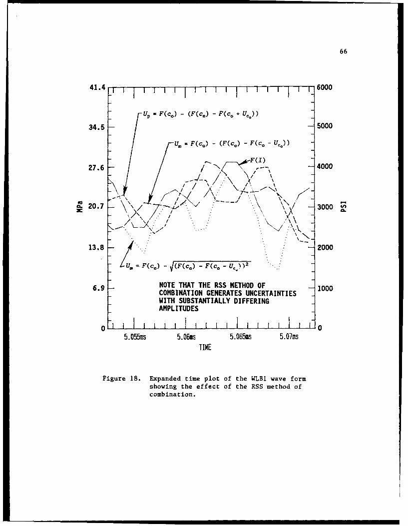
66
41.4 i 6000
Up = F(c0 ) - (F(co) - F(c+ Uo
34.5 5000
Um F(cO) - (F(co) - F(c. - U.))
27.6 /4000
- ,.. . ",, /- \\ / /
20.7 V3000 '
/7.:13.8 -2000
/Ur F(co) _ /(F(c,) - F(c_ U-,))2
6.9 NOTE THAT THE RSS NETHOD OF 1000COMBINATION GENERATES UNCERTAINTIESWITH SUBSTANTIALLY DIFFERINGANPLITUDES
0 - 1 1 1 110
5.055as 5.06ms 5.05ms 5.07msTIME
Figure 18. Expanded time plot of the WLB1 wave form
showing the effect of the RSS method ofcombination.

67
exhibit more error in "phase" than error in amplitude, which is
consistent with the earlier findings. Errors in phase produce little
error in impulse, which was one of the conclusions regarding
uncertainty due to incorrect c,. The RSS method however, as shown in
the dotted trace, produces error in amplitude and is in phase with
F(I). The second term in the equations above represent the error due
to the incorrect co. While the unfolding routine may accurately
calculate its direction to be negative, the squaring/square root
process forces it to be positive. Hence, a positive error is always
subtracted from the unfolded wave form to generate the minus
uncertainty. Accordingly, the minus uncertainty depicted by the dotted
trace (RSS method) is always lower than the unfolded wave form. This
causes the gross error in impulse with the RSS technique.
For combining errors due to uncertainty in wave speed and
reflection coefficients while unfolding bar gage records, the author
suggests using linear combination for the errors due to wave speed and
RSS combination for the errors due to the reflection coefficients.
With this approach, the technique can no longer be labeled "classical"
uncertainty analysis, as it has become specialized for this
application. Mathematically, the plus and minus uncertainties would be
expressed as:
UPIC.A.8 = U,(d lIc,,.u 4' V'Ur(C) JA]2 _ U~t
Ufflc.AB = UFVOICc - 4'UPet 1A]' + [UPMT) ii
This technique of combining errors was incorporated into the unfolding
routine and labeled UNFOLD4 (see Appendix). It is considered to be the

68
best of the unfolding routines, since it combines the errors in the
most reasonable manner. UNFOLD4 was used to unfold the wave forms
studied earlier in this section. Figure 19 shows the unfolded pressure
wave forms for the WLBI record. The only significant difference
between the combination of both error types and that including error
only due to reflection coefficients is a slight increase in the impulse
uncertainties. This is as expected since the uncertainty in impulse
due to incorrect c. was slight.
Dispersion and Other Errors
While errors due to uncertainty in low-frequency wave speed and
reflection coefficients can be addressed analytically or numerically,
errors due to dispersion and other more subtle sources are difficult to
quantify. Dispersion leads to errors in an unfolded wave form in a
manner similar to that of unfolding with an incorrect wave speed.
Dispersion in the bar gage causes the high-frequency portion of the
stress pulse to change shape as it propagates down the bar gage.
Specifically, the high frequency content propagates more slowly down
the bar than the low frequency content. As a result, the rise to peak
is "rolled off", as the low-frequency components outrun the high
frequency peak information and superimpose themselves upon the high
frequency data. As the stress wave travels up and down the bar, the
peak continues to roll off.
To include uncertainty due to dispersion in the unfolding
technique, the variance of wave speed with frequency would have to be
defined and incorporated into the calculational portion of the

- 69
> 0CO -r
C~I 3:-
0.
N U- W 0
<~ r-J U
oc
00
w0.0CX
o~c cc~. 0U
DI I* t I ICV 0 C
ci E Cexcv =0
0.0
rbX 39S X dV
0 0
-. 54 0
w Ui
cr-
E
W)U
CWL
z -4
CV) z
ledNI(0

70
unfolding routine. In turn, the unfolding routine would have to keep
track of the frequency of data which was being handled at each point in
time. This would be a difficult task and is beyond the scope of this
thesis.
If the wave form contains limited high frequency data, dispersion
will not cause significant errors. Also, errors due to dispersion will
manifest themselves much the same way as errors due to incorrect co.
When the routine unfolds the high frequency data, which in most all
cases is limited to the high amplitude initial peak and the subsequent
reflections, it will sum together improper portions of the wave form.
As a result, a noise-like or spiky character would be expected at those
places in the wave form where high amplitude reflections were present.
Such errors are not expezted to produce much error in impulse. In the
unusual case where a bar gage was used to measure a pulse which
contains a great deal of high frequency content, more error may be
inherent to the unfolded wave form. However, the use of a bar gage for
such a high frequency measurement is questionable, even before
considering the validity of unfolded data obtained by the bar gage.
Sometimes the analyst does not know the length of the bar and
position of the strain gages along the bar with precision. Such
precision is unnecessary if the bar gage records are not to be
unfolded, and consequently such precision has often not been applied to
the manufacture of bar gages. The only time that the unfolding routine
uses the bar gage dimensions is in the argument of the functions, just
as was the case with c0 . Consequently, errors due to incorrect bar
gage dimensions lead to the same sort of errors as co, causing the

71
unfolding routine to sum the improper sequence of amplitudes. Gross
errors in bar gage dimensions can be troublesome. For instance, a 6-mm
discrepancy in bar length has the same effect as a 10 m/s error in wave
speed.
The most correct way of handling errors due to bar gage dimensions
would be to perform a separate uncertainty analysis on the arguments of
the functions before using the unfolding program. With the arguments
being composed of simple expressions, this uncertainty analysis would
be easy compared to the analysis performed in this chapter. The
resulting uncertainty for the whole argument, due to the uncertainty in
c., x, and L, could be input to the unfolding program as the
uncertainty in co. Even this thorough of approach has problems though.
Uncertainties in c., L, and x are not independent of one another, i.e.,
x and L are used to determine co. This makes for a more complex and
judgmental uncertainty analysis, and hence it is only mentioned here.
Generally though, if care has been taken in the manufacture of the bar
gages, errors due to incorrect bar gage dimensions should be relatively
insignificant.
Other error sources can be conceived that would effect the
accuracy of the unfolding process. Things such as material variations
throughout the length of the bar gage, material nonlinearities, etc.,
cannot be considered by the unfolding technique, and hence lead to
errors. Such errors are thought to be quite small. Accordingly, they
are not considered in this thesis.
The intent of this chapter is not to suggest that the error
sources discussed here are the only sources of error associated with

72
measurements made by bar gages. Indeed, calibration errors, ground
shock effects, frequency response limitations, etc., lead to errors in
bar gage measurements. Some of these errors will be evident in the
next chapter, where actual field data is examined. However, these
errors are not caused by the numerical unfolding process, which is the
concern of this thesis.

CHAPTER V
APPLICATION OF BAR GAGE UNFOLDING TO
FIELD DATA
Test Description
The uncertainty analysis will be applied to an actual high
explosive test in this chapter. In this experiment, bar gage data was
obtained at regions where other types of blast pressure gages made
measurements as well. This is an unui, :i -A sation because bar gages
are typically used in regions where very few types of airblast gages
can function reliably, due to the high peak pressure levels. On this
test, however, bar gages were intentionally placed at pressure levels
low enough to compare to other airblast gages. The other airblast
gages in this case were Kulite HKS series airblast gages (Reference
11). HKS airblast gages are quite reputable in the peak pressure range
from 3.45 to 345 MPa (500 to 5,000 psi) and, being a diaphragm-type
gage, yield a long term pressure measurement with no interruption from
tensile reflections. Hence, with the Kulite airblast gages being
placed at the same distance as the bar gages from an axisymmetric
charge, the Kulite gage records can be compared to the unfolded bar
gage records.
The experiment of interest involved the detonation of an explosive
charge that was suspended at a certain height above the ground surface.
73

74
Airblast gages were placed on the ground surface to measure the blast
pressure on the ground surface at different radial posiZ.i-s.
Figure 20 is a plan view of the instrument layout. The explosive
charge is suspended above the origin depicted on this plan view. The
bar gages are denoted by Bl, B2, etc., at the pressure ranges close to
the charge. The Kulite pressure gages are denoted by AB15, AB16, etc.
They are located at the same radial distance, and also close to the bar
gages. Bar gage B3 was located at the center of the instrument array.
Bar gages B2, B4, and B6 were located at the same radial distance from
the charge center, arbitrarily referred to as radial "A". Bar gages Bl
and B5 were placed at another radial distance arbitrarily referred to
as radial "B". It is the data from these instruments that is of
interest to us in this thesis. Comparisons will be made between these
bar gages and their corresponding Kulite airblast gages. The
appropriate gage comparisons and their radial positions are presented
in Table 1.
In this chapter, we will compare the records frora those
combinations listed in the previous table. The bar gage records will
be unfolded to the best capability and the uncertainties calculated
using the UNFOLD4 program explained in Chapter 4. The impulses from
the unfolded bar gage records will then be plotted on the same scales
as the Kulite airblast gage impulses. If the gage performance were
similar, then the Kulite airblast impulses would lie within the upper
and lower bounds of the unfolded bar gage impulses. If the Kulite
airblast gage impulses lie outside of these bounds, it means that
either the gages are performing (or measuring) differently, or else

75
0 dog.
A814
RADIAL,
30 - RADIAL B" " ~A 8 1 3 , "AB3C,, ~~A 16--,,-- .," A832 AB 6 " 3 "'Bi B,' 2 • ' 4 ",A . B5A8 1 AB30 M B 1AB 19
AB } A 2AB292 "O AR" A ,15
• , AB27 "" .. 1 5 0
180
Figure 20. Plan view of the pertinent instruments for thesubject explosive test.

76
TABLE 1
BAR GAGES AND KULITE AIRBLAST GAGES ATCOMPARABLE TEST BED POSITIONS.
KULITECOMPARISON RADIAL BAR GAGE AIRBIAST GAGE
NO. POSITION DESIGNATION DESIGNATION
1 CENTER B3 AB15
2 RADIAL A B2 AB29
3 RADIAL A B4 AB16
4 RADIAL A B6 AB28
5 RADIAL B BI AB31
6 RADIAL B B5 AB19
the charge is not producing a uniformly axisymmetric airblast
environment. An analysis will be performed along these lines to see if
any interesting conclusion can be drawn about the accuracy or utility
of bar gage unfolding.
Analysis
The bar gages used on this test were 5.8 m lcng with the strain
gages placed 1.83 m from the top of the bar. This is a standard bar
gage design used on high explosive tests which have no special
measurement requirements, e.g., spatial constraints, long measurement
times, etc. The bar gage records were unfolded using the computer
program UNFOLD4 to calculate both the unfolded wave form, and the
uncertainties due to incorrect wave speed and reflection coefficients.
A low frequency wave speed of 5089 m/sec was found to be the best
choice for these bar gage records (as it was for the other bar gage
types investigated). This value of low-frequency wave speed will

77
likely apply to all bar gages made from the same lot of high-strength
steel. Reflection coefficients and all of the uncertainties were
chosen in a manner consistent with that described earlier.
The results of the unfolding are given in Figures 21 through 26.
The unfolded pressure wave forms, with the plus and minus
uncertainties, are shown in the left-hand plot, while the corresponding
integrated impulses are displayed in the right-hand plot. Two points
are noteworthy from these plots. First, Bl and B5 are peculiar looking
unfolded pressure wave forms when compared to the other unfolded wave
forms. B1 has a repeating pulse, which judging from the timing, is
propagating up and down the bar. This record was unfolded several
times with carefully chosen parameters. The same results were always
achieved. Therefore, it is presumed that Bl was unfolded correctly,
and the oscillations represent a mechanical pulse not due to the
pressure applied to the measurement end of the bar gage.
B5 displays late-time pulses different than that of Bl. The late-
time inputs evident on B5 are not as periodic in nature. These are
above the baselikLe indicating positive pressure. B5 may be responding
to a mechanical input, perhaps from the explosive or some anomalous
behavior in the bar. The other unfolded bar gage records appear to be
reasonable. The uncertainties in the pressure wave form reveal
themselves in the high-frequency spikes at times when the reflections
are being unfolded, as was observed in the previous chapter.
Note that had the records not been unfolded, it is possible that
BI and B5 would not have been singled out as suspect. Since their
initial pulses looked reasonable, and the rest of the records looked

78
o c / .
z. - -,=.
000
o. o
"".- 'I- ".....- - w 1-
* -
00 X Vd
02
.. .. ... ". ...-.......OD ... I....
._• >-• -00 . . --
II ...J. ... .......... l
---------- ---
0 ,, I, ,0 ,, ,I0, -,, , , I. .
-w 0
Wo i o --------
I 0 z v 0 0
o -- X~f I I I
III
~~~ ... . .. ..... .I..III.ll I...II...
It 00ý4-
o LO
0 'IS ----

0o 79
l~~ ~~~~ p -I II ilII
00 j
0
o -""i:
* E
II :), S
co 0))c
I- , - .-
0 0 0
*, , n IM I
o 0obCo
* I
-1
cc x ....... %,
i -
.. . .. . . .. . . . . . .S............ .... ....... D
0A w o a
--0 0 * 0
0 0. 0 W 0
NC
CDC
VdN
0 ,- • •I•I • -- 0a I.I
2• nn m

08
00
o "
o -UI - .- 9.. 4.'
o I .)- •E 0'•:"-E
I :, I . . i i i , , , I . ..I .. . . . 0i0 0 0o M
.. z .i . ..
CO))
w -
S*, ._.a..... _ •
CD U,---
•CD
0;0
Go
44
-. -,
E --
. ..D u0.
x>cc - 0
o) ,-, --,,-,-- ----- - -
UoII o • I o - o - - - 0
Ci 0 co W• W• 44u• •
-- LL I I
ua. . . .. . .......... 0..I
N ...DIA.
2)~hi
oi to 0-U to to0. to

81
o.o.0
00
<0 0- -
II 5.4 ,. 0 :v
D o ,o CO
LJ co J - .• .. •"
S.,.
0 000
t , . . . ..I I I ., .
00
11-
Lii 0 0 6 06 0* 0 i, 0. 6J • •
44 -
ODC
N..
Eii
zdl-4
C14
0 0
10
No to 0 Lo 0 Ic) 0 ILOU 0 Il- Lo N~ N~ Ito
'edVi

82CDO
00w Wo _,
4 0
o -. ,,1-I.1
I-.0>I \,"b,-.•
q,, • -. 1 - w.
to
oI I t a I
1..• q• -w "
W D to tc 0
0)0
r: 0
0 0
0 °
•1"G -' d r --- 0,..4
4 1 0
I.- I o o 0o 0 0 0 r
4 0 l• 0 O9Xd O U
--- -I
E 04
CD ...........44 4
~~u ....... i4)llI•11||[ l
0
-- 47
E
"1? 00n0 t o 0 t
'Rd-a

83
". I n
S 4J- 0 w44
E crL5 m .)
D 00
o 1:o
C O 00
I• - I- IllIII . I' .i-
UU
. OOS X •cVd•ca
' '-a
A. .Aw 4a 1~~............. . ....,,- ...... I.. ....... -.-.' -0 • m•_ ......... .... ... . -....... ,.,E .................... --.. _.-....-....
, ~ ~ ~~~~..... ....... I'" .........
E 1
. ..... .. ......... % 0
D ........ , I , • ...... . cc
c.J
-S '-).0U m O •
t t i
0~edW

84
"bar gage-like", it would be easy to conclude that records were valid.
By unfolding the records, the differences became obvious. With regard
to this example, it is concluded that unfolding the bar gage records
can be useful in evaluating the quality of the bar gage measurement.
The uncertainties due to the reflection coefficients yield large
uncertainties in the unfolded impulses. This is a second noteworthy
point regarding the unfolding of these bar gage records. Even the most
careful examination of the bar gage records could not yield a constant
reflection coefficient. The reflection coefficient varied as much as
eight percent, requiring that amount of uncertainty to be input to the
unfolding program. As can be seen in Figure 23, these sorts of
uncertainties in reflection coefficients cause gross errors in the
unfolded impulse. An analyst could only use one or two reflections of
an unfolded impulse wave form with uncertainties that large. Some of
the records had less uncertainty in their reflection coefficients and
the unfolded impulse waveforms are more reasonable. B5 and B6 in
Figures 25 and 26 are good examples of this.
Each unfolded bar gage record is plotted along with its
corresponding Kulite airblast gage record in Figures 27 through 32. As
before, the pressure wave forms are grouped together on one plot and
the integrated impulses on another. The plus and minus uncertainties
of the unfolded pressure wave form are left off of these plots for
clarity. The airblast data from the Kulite airblast gages required
little or no data manipulation. Prior to making these plots, 100-ms
plots of the Kulite airblast data were studied to determine the maximum

-r 85
t~i
0&
LL L,.,ZDLAn ,. L) CO-
U Z $4
4-4
ca - CLO
o ~41
N insn o-4N Co
9ý 0Sn
0
00
S -4 g
Of UU (u
a4 0 44.co
0U w
0:0y
oo ww
'44
I t04J

86
Q~ý- 4 1w4J
co w -C
mV~~L -I,'.- w u-Wi L~L) JV
d ~ Z _j
CL 0
0 of)
a- * . a a a I aces zLa ,.. D
lc 0
4.40
0
w CNJ
00
L) 0
an,o c
an ~cn~ -
00 ~CL aAL) mi
iinUC
o 00

tfl 87Lni
41
00C;w
0 Ln 0
a 0
M) Zm a,-= . I- L
W .
U)n ~ U)0IV 0 - en
0 0 0
00
0
0
m cc
D O0 -4:
00 W ci =-w
0jý 0 H
E, 0 c
0Y 0ý UU ,
eEc'

f 88
00
00
-~f n
CL)
UU
ca
cc 0
LIl-
E 0
141
-r 14. c
4o0-
E 0 <' I r
C'.'
L) .11
4 ~~14-0nt
LaJ ~fl4EN _? L
'.a.OdJ

89In
w
cs ~w w
U) M
j LO
C))C U r
-U 6
ci 0
U) 'aWV)f
LO~ !z
~co
0.
ir0-a
0 4
0c) C0U.0 0i vu o 40 1
8 l an LO n b
r- Lo 04 dV r

90
o II u-
I-. On. z~IU **
co C 0
tn 0
.q.1
i~Lt) to q
- 0-
0 0 C0
N 04-4
- ca
w-c -
LX Ecn 0-4
wow cc -
C4
in 61) n L
k4
8edVYI

91
pulse lengths. It was determined that 16-ms plots would be adequate to
display all of the useful data. Since the Kulite airblast gage trace
returns to the baseline (zero pressure) and stays there, the dashed
trace is difficult to see on the pressure plots.
Impulses from the unfolded bar gage records range from 40 to 100
percent higher than the impulses measured by the Kulite airblast gages.
With differences this extreme, the impulses measured by the Kulite
airblast gages remain well below the minus uncertainty in the unfolded
wave forms. Recall that numerical unfolding leaves the portion of the
wave form prior to the first tensile reflection untouched. In each of
Figures 27 through 32 the impulse measured by the bar gage exceeds the
impulse measured by the Kulite airblast gage well before the first
reflection is unfolded. Hence, the discrepancy between the two gage
types is established before numerical unfolding can contribute. For
these reasons, numerical unfolding could not have caused the
discrepancies between the two gage types.
Because the bar gages were located close to their companion Kulite
airblast gage, it is highly unlikely that the pressure field generated
by the symmetric charge caused the systematic differences observed by
the two gage types. These differences appear to fall well outside of
data scatter (see, for example the Kulite and bar gage measurements
along Radial A). Therefore, one can conclude that the discrepancies
between gage types are not due to position in the test bed, or just
excessive scatter in the data.
The likely cause for differences between gage types is some
fundamental difference in the measurement techniques. Observe the

92
pressure plots. The bar gage recoreds indicate a second pressure pulse
arriving about 0.5 to 1.2-msec after the arrival of the primary
pressure pulse. This second pulse is not evident on the wave forms
measured by the Kulite airblast gages. Since this second pulse on the
bar gage records has substantial amplitude and duration, it affects the
impulse significantly. This second pulse accounts for the difference
in impulse measured by the two gage types.
Recent analysis of the data indicate that the bar gages are in
error, i.e., the second pulse is not representative of the actual
pressure environment at the end of the bar gage (Reference 12). It has
been hypothesized that ground shock loadings, water jacket effects, or
shear loads induced by relative motion between the bar and the
surrounding jacket, might cause the peculiar bar gage output.
For completeness, it should be pointed out that there is no
guarantee that the unfolding routine will correctly unfold data that is
input to the lateral surfaces of the bar gage. Hence, from a purist
point of view, errors due to poor bar gage performance can also be
unfolded incorrectly and contribute to further unfolding errors.
Future research and development will likely lead to bar gage designs
which minimize influences from lateral loadings. In the absence of
lateral loading induced errors, the uncertainties due to wave speed and
reflection coefficients are the primary sources of error in the
unfolding routine.
While the numerical unfolding of the these bar gage records was
not necessary to reveal the differences between the two types of
airblast gages, this application demonstrates how numerical unfolding

93
can be used during data analysis. Had there been no grievous
differences between the gage types, more profound conclusions might
have been made. In general, numerical unfolding with the calculated
uncertainties can be used for the following purposes during data
analysis:
1. Determine for each individual wave form the length of unfolded
bar gage record that can be used without incurring too much
error.
2. Gain insight into the quality of the bar gage record. Bar
gage records of good quality tend to produce predictable wave
shapes when unfolded.
3. Allow comparisons with other airblast gages having longer
duration records. If other wave forms lie outside of the
error bounds of the numerical unfolding, the discrepancy is
due to some source other than the numerical unfolding. If the
wave forms lie inside the error bounds of the numerical
unfolding, then it is possible that discrepancies are due to
the unfolding and further explanations for the discrepancies
must be presented carefully, or withheld all together.

CHAPTER VI
CONCLUSIONS
Review
Bar gages are frequently used to measure airblast on explosive
tests. The unique design and configuration of a bar gage allows it to
measure high peak pressure and impulse close to an explosive charge.
Unfortunately, the arrival of reflections from the ends of the bar gage
limit the length of time that the primary pressure pulse can be
measured. In this thesis we investigated the errors associated with
the use of D'Alembert unfolding to numerically remove the reflections
from the bar gage record, thereby restoring the original pressure
pulse.
D'Alembert unfolding is a numerical technique by which the tensile
reflections from the bottom of the bar gage, and the compressive
reflections from the top of the bar gage, are added and subtracted from
the measured wave form in such a way as to restore the original
pressure pulse. The numerical technique makes the same assumptions as
D'Alembert did in formulating his classical wave propagation equation.
The most notable assumption being that the pulse propagates up and down
the bar at a constant wave speed without changing shape. By further
assuming that accurate and constant reflection coefficients can be
identified for the ends of the bar gage while it makes the measurement,
94

95
the reflections can be subtracted from the measured wave form. In
1983, computer programs were written to perform this numerical
technique on actual bar gage records.
Although D'Alembert unfolding often yielded reasonable results,
critics pointed out potential flaws in the technique. Dispersion in
high-frequency data is contrary to the principle assumptions on
D'Alembert unfolding; namely, the wave speed varies with frequency
content, and hence the pulse changes shape as it propagates down the
bar. Also, reflection coefficients seem to vary thioughout the record
slightly. By assuming a constant reflection coefficient for each end
of the bar, considerable error could be introduced into the numerical
result. It was argued that this error could cause large errors in
specific impulse (first integral of pressure), a very important
quantity for explosive testing. Alternatively, proponents of unfolding
indicated that if even one reflection could be unfolded with acceptable
error, it would greatly increase the value of the bar gage measurement.
This thesis sought to quantify the errors inherent to D'Alembert
unfolding, permitting a sound judgement to be made regarding the
credibility of the numerical technique.
The governing equation for D'Alembert unLolding was examined and
three error sources were chosen for study. These error sources (listed
below) comprise most of the error in the unfolding technique:
1. Specifying incorrect low frequency wave speed, co.

96
2. Choosing incorrect reflection coefficients, or assuming
constant reflection coefficients when in reality, reflection
coefficients were changing.
3. Dispersion and incorrect bar gage dimensions.
The first two errors were addressed analytically and numerically
to arrive at the uncertainty in the unfolded wave form. The last
errors were merely discussed to qualitatively assess their
significance.
Recent experiments, suggest that bar gage output may be influenced
by lateral loading during high expl sive tests. The purpose of the bar
gage and the unfolding routine are to deduce the pressure loading at
the end of the bar. Lateral loads originate at places other than the
end of the bar and propagate away hence forth. The unfolding routine
is not designed to correct for these sorts of input. It is conceivable
that the unfolding routine could generate further errors when used on
bar gage records generated by multiple loading sites. Determination or
treatment of errors induced by lateral loading are beyond the scope of
this thesis. In, the absence of such lateral loading errors, the
uncertainty analysis presented in this thesis has addressed the primary
error sources.
Errors in the unfolded wave form due to uncertainty in the wave
speed were identified numerically. Upper and lower bounds were placed
on the wave speed, and the wave form unfolded for each case. The
uncertainty in the unfolded wave form due to uncertainty in wave speed
was then simply the difference between the wave forms.

97
Errors in the unfolded wave form due to uncertainty in the
reflection coefficients were determined analytically by applying
classical uncertainty analysis to the mathematical expression for the
unfolded wave form. This yielded exact expressions for the uncertainty
due to reflection coefficients, which could then be applied to specific
wave forms.
The effect of tne,7c errors was then examined by unfolding
candidate wave Forms and calculating the uncertainty due to both error
sources individually. Two types of wave forms were used. The first
type, was a zecord from a ball drop calibzation on a specially made bar
gage where all of the dimensions were precisely known. The ball drop
calibration is a controlled laboratory test. The input to the bar gage
from a ball drop calibration is well known and is complete before the
first tensile reflection arrives. Consequently, it was a good choice
for evaluating the effect of unfolding errors. Ball drop calibrations
also have lower frequency content, so dispersion is not prevalent.
The second type of wave form was a typical high explosive test
record, specifically the WLB-I record. Unfolding this wave form
revealed the effect of the individual uncertainties on a wave form
which contained considerable high frequency content. The wave form
from the high explosive test also had larger uncertainties in
reflection coefficients, which is typical of most explosive test data.
Therefore, this wave form was representative of practical applications.
The proper method for combining these two errors; i.e., that due
to uncertainty in wave speed, and that due to uncertainty in reflection
coefficierg.s, was then studied. It was determined that adding the

98
uncertainty due to incorrect wave speed to the RSS combination (square
root of the sum of the squares) of the uncertainties due to the
reflection coefficients was the best method of arriving at the total
uncertainty of the unfolded wave form. This was incorporated into a
computer program that calculated the uncertainties for the specific
wave form of interest. In this way, upper and lower bounds on the true
unfolded wave form could be established for the data analyst.
This error analysis was applied to airblast data from a candidate
high explosive test. This test allowed for the comparison of unfolded
bar gage records with another reputable type of airblast gage, the
Kulite HKS airblast gage. All of the bar gage records were unfolded
and then compared to their Kulite airblast gage counterpart. This
analysis demonstrated the D'Alembert unfolding technique upon actual
field test data and revealed systematic differences between bar gage
measurements and the Kulite HKS airblast gage.
Conclusions
Several conclusions are drawn from this study. They are:
1. An uncertainty analysis method was developed which
treats the uncertainties inherent in the
D'Alembert unfolding technique as applied to
strain-gaged Hopkinson bar gage records. A
modified unfolding program was written which
provides the analyst with the useful upper and
lower bounds of uncertainty for a particular wave

99
form. The magnitude of the uncertainty is wave
form specific, i.e., dependent on the character of
the particular wave form being analyzed.
2. Errors in the reflection coefficients may yield
large errors in unfolded impulse. These errors
are the primary factor limiting the usefulness of
D'Alembert unfolding. With the unfolding of
subsequent reflections, the error in impulse from
these sources increases geometrically.
3. Errors in wave speed produce spikes on the
unfolded pressure wave form, but do not yield
large errors in impulse. In general, with higher
frequency content airblast data, and with larger
uncertainty in wave speed, the spiky, noise-like
behavior will be more prevalent.
4. Dispersion, uncertainties in bar Saie dimensions,
and other errors are less significant, and
manifest themselves in a manner similar to errors
in wave speed.
5. The differences between the unfolded bar gage
measurements and Kulite airblast measurements are
not due to errors in the D'Alembert unfolding
technique. Evidence suggests that bar gage
measurements were influenced by phenomena other
than airblast (e.g., lateral loading), and that

100
the Kulite airblast gages were not affected by
these phenomena.
6. Unfolding bar gage records can aid the data
analyst in assessing the quality of the bar gage
measurement. Peculiar behavior that is "hidden"
in the reflections sometimes is revealed by
D'Alembert unfolding.
These conclusions assume that the analyst has made reasonable
choices of wave speed and reflection coefficients, and the
uncertainties associated with these parameters. Performing D'Alembert
unfolding with grossly incorrect parameters or very large uncertainties
can lead to results which are contrary to the above conclusions.
Recommendations
The objective of this thesis was to ascertain the credibility of
D'Alembert unfolding as a data reduction technique for bar gage
records. The error analysis of the D'Alembert unfolding method
accomplished that objective by quantifying the errors due to unfolding
a particular wave form. This error analysis included only the effects
of uncertainty in wave speed, reflection coefficients, and dispersion.
If other significant sources of error are found, effort should be made
to incorporate these errors into the uncertainty calculations.
The most important recommendation from this work is to apply the
modified D'Alembert unfolding program to more field data. As was
eluded to in earlier chapters, bar gages exhibit phenomena which are
not fully understood. By unfolding the bar gage records and comparing

101
them to other airblast measurements, bar gage performance might be
better understood. Having the upper and lower bounds on the numerical
unfolding errors, the analyst can confidently choose the length of
unfolded record to use and assess the validity of its comparison to
other measurements or predictions.

APPENDIX
This appendix contains the computer program listings for the
unfolding programs used in this thesis. Refer to Chapter 3 for a
description of the basic organization of these codes. A flow chart of
the basic workings of these programs is shown in Figure 8 of Chapter 3.
The computer program UNFOLD is essentially the same program
developed by Welch and White for operation on Tektronics and VAX
computer systems. This program was modified to run on IBM personal
computers and compatibles for this thesis, and named UNFOLD. UNFOLD1
uses the first program as its core, but also calculates a plus and
minus uncertainty in the unfolded wave form due to uncertainty in wave
speed. UNFOLD2 uses the first program as its core, but calculates plus
and minus uncertainty in the unfolded wave form due uncertainties in
both reflection coefficients. UNFOLD4 is the final program developed
for this thesis. UNFOLD4 combines the uncertainties in the unfolded
wave form due to wave speed and reflection coefficients.
The computer program UNFOLD3 is conspicuously missing from this
appendix. UNFOLD3 was written to identify the differences between two
different schemes of combining the uncertainties in the unfolded wave
form due to both wave speed and reflection coefficients. UNFOLD3 was
subsequently used to generate the data for Figure 18 (Chapter 4). One
of those schemes was deemed inappropriate. Accordingly, the listing of
102

103
UNFOLD3 is not included in this thesis to avoid confusion.
The listings of UNFOLD, UNFOLD1, UNFOLD2, and UNFOLD4 follow this
narrative in their respective order.

104
PROGRAM UNFOLD
C*****REVISED ON 10-13-90 TO MAKE THE PROGRAM MORE EFFICIENT***
C*****ROUTINE NOW DISCERNS WHICH REFLECTION POINT "1" IS IN****
C*****AND ONLY RUNS LOOP THAT MANY TIMES. OTHER THINGS ARE****
C*****TO MAKE PROGRAM M )RE LOGICAL AND EFFICIENT. MORE********
C*****COMMENTS STATEMENTS ARE ADDED FOR CLARITY****************
C*****INITIAUZE AND DEFINE SOME VARIABLES AND ARRAYS**********
CHARACTER*30 BARFILE1,BARUNFOLD
PARAMETER (NN =17000)
DIMENSION A(NN), F(NN)
NFIRST=4.
C*****INPUT BAR GAGE PARAMETERS AND OTHER INFORMATION**********
PRINT*,'INPUT WAVE SPEED OF BAR (FT/S)
READ(*,*) C
PRINT*,'INPUT LENGTH OF BAR (FT)
READ(*,*) BARLEN
PRINT*,'INPUT DISTANCE BETWEEN TOP OF BAR AND GAGE (FT)
READ(*,*) X
PRINT*,'iNPUT REFLECTION COEFFICIENT FOR DUMP END OF BAR
READ(*,*) GAMMA1
PRINT*,'INPUT REFLECTION COEFFICIENT FOR INPUT END OF BAR
READ(*,*) GAMMA2

105
PRINT*,'INPUT TIME OF ARRIVAL (SEC)
READ(*,*) TOA
PRINT*,'WHAT IS NAME OF BAR GAGE DATA FILE TO UNFOLD?
READ(*,1000) BARFILE1
PRINT*,'WHAT IS NAME OF FILE FOR UNFOLDED DATA?
READ(*,1000) BARUNFOLD
PRINT*,'HOW MANY TENSILE REFLECTIONS ARE THERE?
READ(*,*) NREFL
C*****OPEN FILES, READ HEADER INFORMATION***********************
OPEN(1 5,FILE = BARFILE1 ,STATUS ='OLD',FORM = 'FORMATTED')
OPEN(1 6,FILE = BARUNFOLD,FORM ='FORMATTED')
READ(15,2000) TFIRST,TINC,FKOUNT
WRITE(16,2000) TFIRST,TINC,FKOUNT
KOUNT=-IFIX(FKOUNT)
C*****UNFOLD WAVEFORM*******************************************
TWOC=2./C
DO 100 I=NFIRST,KOUNT
G2=0.0
G2=0.0

106
DO 200 N =1 ,NREFL
TEMP =TWOC*(FLOAT(N)*BARLEN-X)
VALl = TIME-TEMP-TOA
IF(VAL1 .GT.O) THEN
J = IFIX(TEMP[TINC)
J=-IJ
IF(J.GT.0) THEN
IF(J.GE.NFIRST) THEN
Gi = Gi +(GAMMAl **N)*(GAMMA2**(N-1 ))*F(J)
TEMP =TWOC*FLOAT(N)*BARLEN
VAL2 =TIME-TEMP-TOA
IF(VAL2.GT.0) THEN
J =IFIX(rEMP/TINC)
J =I-J
IF(J.GT.0) THEN
IF(J.GE.NFIRST) THEN
G2=G2+ (GAMMA1**N)*(GAMMA2**N)*F(J)
END IF
END IF
END IF
END IF
END IF
END IF
200 CONTINUE

107
READ(15,*) TIME, A(I)
F(I) =A(I)+G1-G2
WRITE(16,4000) TIME, F(I)
100 CONTINUE
50 CLOSE (UNIT= 15)
CLOSE (UNIT= 16)
C*****FORMAT STATEMENTS*****************************************
1000 FORMAT(A30)
2000 FORMAT(E12.4,/,E12.4,/,E12.4)
3000 FORMAT(E12.4)
4000 FORMAT(F10.8,IX,F12.5)
END

108
PROGRAM UNFOLD1
C*****THIS PROGRAM CALCULATES UPPER AND LOWER BOUND *
C*****UNFOLDED WAVEFORMS FOR SPECIFIED CHANGES IN WAVE *******
C*****SPEED. THREE WAVEFORMS ARE OUTPUT, UNFOLDED *
C*****WAVEFORM, PLUS AND MINUS UNCERTAINTY*********************
C*****REVISED ON 11-26-90 TO MAKE THE PROGRAM MORE EFFICIENT***
C*****ROUTINE NOW DISCERNS WHICH REFLECTION POINT I" IS IN****
C*****AND ONLY RUNS LOOP THAT MANY TIMES. OTHER THINGS ARE****
C*****TO MAKE PROGRAM MORE LOGICAL AND EFFICIENT. MORE********
C*****COMMENTS STATEMENTS ARE ADDED FOR CLARITY****************
C*****INITIAUZE AND DEFINE SOME VARIABLES AND ARRAYS**********
CHARACTER*30 BARFILE1 ,BARUNFOLD,MINUSUNC,PLUSUNC
PARAMETER (NN= 16000)
DIMENSION A(NN), F(NN)
DIMENSION G1(3), G2(3)
NFIRST=4.
C*****INPUT BAR GAGE PARAMETERS*********************************
PRINT*,'INPUT WAVE SPEED OF BAR (FT/S)
READ(*,*) C
PRINT*,'INPUT UNCERTAINTY OF WAVE SPEED (+ /- X" FT/S)
READ(*,*) UC

109
PRINT*,'INPUT LENGTH OF BAR (FT)
READ(*,*) BARLEN
PRINT*,'INPUT DISTANCE BETWEEN TOP OF BAR AND GAGE (FT)
READ(*,*) X
PRINT*,'INPUT REFLECTION COEFFICIENT FOR DUMP END OF BAR
READ(*,*) GAMMAl
PRINT*,'INPUT REFLECTION COEFFICIENT FOR INPUT END OF BAR'
READ(*,*) GAMMA2
PRINT*,'INPUT TIME OF ARRIVAL (SEC)
READ(*,*) TOA
PRINT*,'WHAT IS NAME OF BAR GAGE DATA FILE TO UNFOLD?
READ(*,1000) BARFILE1
PRINT*,'WHAT IS NAME OF FILE FOR UNFOLDED DATA?
READ(*,1000) BARUNFOLD
PRIN'T*,'WHAT IS NAME OF FILE FOR MINUS UNCERTAINTY?
READ(*,1000) MINUSUNC
PRINT*,'WHAT IS NAME OF FILE FOR PLUS UNCERTAINTY?
READ(*,1000) PLUSUNC
C*****OPEN FILES, READ HEADER INFORMATION***********************
OPEN(1 5,FILE = BARFILE 1,STATUS = 'OLD',FORM = 'FORMATTED')
OPEN (1 6,FILE = BARUNFOLD,FORM = 'FORMATTED')
OPEN(17,FILE = MINUSUNC, FORM ='FORMATTED')
OPEN(18,FILE = PLUSUNC, FORM = 'FORMATTED')

110
READ(15.2000) TFIRSTTINC,FKOUNT
WRITE(1 6,2000) TFIRST,TINC,FKOUNT
KOUNT= IFIX(FKOUNT)
C*****UNFOLD WAVEFORM*******************************************
DO 100 I= NFIRST,KOUNT
READ(15,*,END=50) TIME, A(I)
DO 125 L=1,3
Gi (L)=zO.o
G2(L) =0.0
125 CONTINUE
DO 150 K = 1,3
IF (K1.EQ.1) THEN
Cl =C-UC
ELSE IF (KI.EO.2) THEN
Cl =C
ELSE IF (Ki .EO.3) THEN
Cl =C+UC
ENDIF
C*****IF 1" LIES PRIOR TO FIRST TENSILE REFLECTION, WRITE******
C***** POINT DIRECTLY TO OUTPUTFIE***********

TWOC=2./CI
IF (TiME.LT.(TOA +TWOC*(BARLEN-X))) THEN
GO TO 5
ELSE
C*****IF "I" LIES AFTER FIRST TENSILE REFLECTION, FIND**********
C*****OUT WHICH REFLECTION IT UIES IN, AND SET VARIABLE *N"*****
C*****TO THAT NME**********************
DIF =(TIME-(TOA +TWOC* (BARLEN.X)))/(TWOC*BARLEN)
WNUM =AINT(DIF)
DEC =DIF-WNUM
IF (DEC.LT.O.50) THEN
DIF=DIF+O.50
ENDIF
N =NINT(DIF)
ENDIF
C*****PERFORM SUMMATIONS OF SECOND TERM*************************
DO 200 K= 1.N
TEMP = (2./Cl )*(FLOAT(K)*BARLEN-X)
J = IFIX(TEMP/TINC)
J =I-J
Gi (Ki) = Gi (KI) + (GAMMA1 **K)*(GAMMA2** (K-l ))*F(J)

112
C*****DETERMINE IF SUMMATIONS OF THIRD TERM ARE NECESSARY, *
C*****AND IF SO, PERFORM TE***********************************
TEMP = (2./Cl)*FLOAT(K)*BARLEN
VAL2 =TIME-TEMP-TOA
IF(VAL2.GT.0) THEN
J = IFIX(TEMP/TINC)
J=I-J
G2(Kl) = G2(K1) + (GAMMAI **K) *(GAMMA2**K) *F(J)
END IF
200 CONTINUE
150 CONTINUE
C*****COMPUTE AMPUTUDE OF UNFOLDED VALUE OF POINT a"" AND *****
C*****WRITE IT TO THE OUTPUT ********************************
5 F(I) =A(I) +Gl (2)-G2(2)
FMINUS=A(I) +G1 (l)-G2(1)
FPLUS =A(I) + Gi (3)-G2(3)
WRITE(16,4000) TIME, F(I)
WRITE(17,4000) TIME, FMINUS
WRITE(18,4000) TIME, FPLUS
100 CONTINUE

113
50 CLOSE (UNIT=15)
CLOSE (UNIT= 16)
CLOSE (UNIT= 17)
CLOSE (UNIT= 18)
C*****FORMAT STATEMENTS*****************************************
1000 FORMAT(A30)
2000 FORMAT(E12.4,/,E12.4,/,E12.4)
3000 FORMAT(E12.4)
4000 FORMAT(F10.8,1X,F12.5)
END

114
PROGRAM UNFOLD2
C*****PROGRAM IS THE SAME AS UNFOLD EXCEPT THAT IT ALSO*****
C*****CALCULATES THE UNCERTAINTY IN THE UNFOLDED WAVEFORM***
C*****DUE TO THE UNCERTAINTY IN THE REFLECTION COEFFICIENTS*
C*****REVISED ON 11-12-90 TO INCORPORATE CHANGES WHICH MAKE*
C*****PROGRAM MORE LOGICAL AND EFFICIENT."""**********'*****
C*****INITIALIZE AND DEFINE SOME VARIABLES
CHARACTER*30 BARFILE1,BARUNFOLD,UNCFILEP,UNCFILEM
PARAMETER (NN = 17000)
DIMENSION A(NN), F(NN)
NFIRST=4.
C*****INPUT BAR GAGE PARAMETERS*********************************
PRINT*,'INPUT WAVE SPEED OF BAR (FT/S)
READ(*,*) C
PRINT*,'INPUT LENGTH OF BAR (FT)
READ(*,*) BARLEN
PRINT*,'INPUT DISTANCE BETWEEN TOP OF BAR AND GAGE (FT)
READ(*.*) X
PRINT*,'INPUT REFLECTION COEFFICIENT FOR DUMP END OF BAR
READ(*,*) GAMMA1

115
PRINT*,'UNCERTAINTY OF THE DUMP END REFL. COEFFICIENT
READ(*,*) UA
PRINT*,'INPUT REFLECTION COEFFICIENT FOR INPUT END OF BAR' READ(*,*)
GAMMA2
PRINT*,'UNCERTAINTY OF THE INPUT END REFL COEFFICIENT
READ(*,*) UB
PRINT*,'INPUT TIME OF ARRIVAL (SEC)
READ(*,*) TOA
PRINT*,'WHAT IS NAME OF BAR GAGE DATA FILE TO UNFOLD?
READ(*,1000) BARFILE1
PRINT*,'WHAT IS NAME OF FILE FOR UNFOLDED DATA?
READ(*, 1000) BARUNFOLD
PRINT*,'GIVE A FILENAME FOR THE PLUS UNCERTAINTY VALUES
READ(*,1000) UNCFILEP
PRINT*,'GIVE A FILENAME FOR THE MINUS UNCERTAINTY VALUES
READ(*,1000) UNCFILEM
C*****OPEN FILES, READ HEADER INFORMATION***********************
OPEN(1 5,FILE= BARFILE1,STATUS ='OLD',FORM ='FORMATTED')
OPEN(16,FILE = BARUNFOLD,FORM = 'FORMATTED')
OPEN(1 7,FILE = UNCFILEP,FORM = 'FORMATTED')
OPEN(1 8,FILE = UNCFILEM,FORM = 'FORMATTED')

116
READ(1 5,2000) TFIRSTTINC,FKOUNT
WRlTE(l 6,2000) TFIRST.TINC,FKOUNT
WFRITE(l 7,2000) TFIRSTTINC,FKOUNT
WRITE(1 8,2000) TFIRST,TINC,FKOUNT
KOUNT= IFIX(FKOUNT)
C*****UNFOLO WAVEFORM*******~************************************
TWOC=2./C
D0 100 I=NFIRST,KOUNT
READ(15,*,END=50) TIME, A(I)
G1 =0.0
G2=0.0
Al =0.0
A2 =0.0
61 =0.0
B2 = 0.0
C*****IF 01" LIES PRIOR TO FIRST TENSILE REFLECTION, WRITE******
C*** POINT DIRECTLY TO OUTPUT FL**************
IF (TIME.LT. (TOA +TWOC*(BARLEN-X))) THEN
GO TO 5

117
ELSE
C*****IF "I" UIES AFTER FIRST TENSILE REFLECTION, FIND**********
C*****OUT WHICH REFLECTION IT UIES IN, AND SET VARIABLE "N******
C*****TO THATNU ER*********************
DIF= (TIME-(TOA+ TWOC*(BARLEN-X)))/(TWOC*BARLEN)
WNUM =AINT(DIF)
DEC =DIF-WNUM
IF (DEC.L.T.O.5O) THEN
DIF=DIF+O.50
ENDIF
N =NINT(DIF)
ENDIF
C*****PERFORM SUMMATIONS OF SECOND TERM*************************
DO 200 K=l1,N
TEMP =TWOC*(FLOAT(K)*BARLEN-X)
J =IFIX(TEMP/TINC)
J =I-J
Gi =Gl + (GAMMAl**K)*(GAMMA2**(K-l))*F(J)
Al = Al + K*(GAMMAI **(K-l)) *(GAMMA2**(K-1))*F(J)
Bi =61 + (K-l)*(GAMMAl**K)*(GAMMA2**(K-2))*F(J)

118
C*****DETERMINE IF SUMMATIONS OF THIRD TERM ARE NECESSARY,
C*****AND IF SO, PERFORMTHM*****************
TEMP =1WOC*FLOAT(K)*BARLEN
VAL2 =TIME-TEMP-TOA
IF(VAL.2.GT.O) THEN
J =IFIX(TEMP/TINC)
J =I-J
G2 =G2 +(GAMMAl **Kq*(GAMMA2**K)*F(J)
A2 =A2 +K*(GAMMA1 **(Kl ))*(GAMMA2**K)*F(J)
82 =B2 +K*(GAMMA1 **Kq*(GAMMA2**(K-i1))*F(J)
END IF
200 CONTINUE
C*****COMPUTE AMPLITUDE OF UNFOLDED VALUE OF POINT *I' AND
C*****WRITE IT TO THE OUTPUT FL***************
5 F(I)=A(I)+Gl-G2
UNCA= ((Al .A2)/F(I))*UA
UNCB = ((81 -B2)/F(i))*UB
U = ((UNCA**2) + (UNCB**2))**0.5
UP = F(t) + (U*ABS(F(I)))
UM = F(i)-(U*ABS(F(I)))

119
WRITE(16,4000) TIME, F(I)
WRITE(1 7,4000) TIME, UP
WRITE(18,4000) TIME, UM
100 CONTINUE
50 CLOSE (UNIT= 15)
CLOSE (UNIT= 16)
CLOSE (UNIT= 17)
CLOSE (UNIT= 18)
C*****FORMAT STATEMENTS*****************************************
1000 FORMAT(A30)
2000 FORMAT(E12.4,/,E12.4,/,E12.4)
3000 FORMAT(11X,E12.4)
4000 FORMAT(F1O.8,1X,F12.5)
END

120
PROGRAM UNFOLD4
C*****THIS PROGRAM CALCULATES UNCERTAINTY DUE TO C, A, AND B,****
C*****AND WRITES THE PLUS AND MINUS UNCERTAINTIES TO A FILE.*****
C*****REVISED ON 11-26-90 TO MAKE THE PROGRAM MORE EFFICIENT***
C*****ROUTINE NOW DISCERNS WHICH REFLECTION POINT -I- IS IN****
C*****AND ONLY RUNS LOOP THAT MANY TIMES. OTHER THINGS ARE****
C*****TO MAKE PROGRAM MORE LOGICAL AND EFFICIENT. MORE********
C*****COMMENTS STATEMENTS ARE ADDED FOR CLARITY****************
C*****INITIALIZE AND DEFINE SOME VARIABLES AND ARRAYS**********
CHARACTER*30 BARFILE1 ,BARUNFOLD,MINUSUNC,PLUSUNC
PARAMETER (NN= 16000)
DIMENSION A(NN), F(NN)
DIMENSION G1(3), G2(3)
NFIRST=4.
C*****INPUT BAR GAGE PARAMETERS*********************************
PRINT*,'INPUT WAVE SPEED OF BAR (FT/S)
READ(*,*) C
PRINT*,'INPUT UNCERTAINTY OF WAVE SPEED (+ /- "X" FT/S)
READ(*,*) UC
PRINT*,'INPUT LENGTH OF BAR (FT)

121
READ(*,*) BARLEN
PRINT*,'INPUT DISTANCE BETWEEN TOP OF BAR AND GAGE (FT)
READ(*,*) X
PRINT*,'INPUT REFLECTION COEFFICIENT FOR DUMP END OF BAR'
READ(*,*) GAMMA1
PRINT*,'UNCERTAINTY OF THE DUMP END REFL COEFFICIENT
READ(*,*) UA
PRINT*,'INPUT REFLECTION COEFFICIENT FOR INPUT END OF BAR'
READ(*,*) GAMMA2
PRINT*,'UNCERTAINTY OF THE INPUT END REFL. COEFFICIENT
READ(*,*) UB
PRINT*,'INPUT TIME OF ARRIVAL (SEC)
READ(*,*) TOA
PRINT*,'WHAT IS NAME OF BAR GAGE DATA FILE TO UNFOLD?
READ(*,1000) BARFILE1
PRINT*,'WHAT IS NAME OF FILE FOR UNFOLDED DATA?
READ(*.1000) BARUNFOLD
PRINT*,PWHAT IS NAME OF FILE FOR MINUS UNCERTAINTY?
READ(*,1000) MINUSUNC
PRINT*,WHAT IS NAME OF FILE FOR PLUS UNCERTAINTY?
READ(*,1000) PLUSUNC
C*****OPEN FILES, READ HEADER INFORMATION***********************
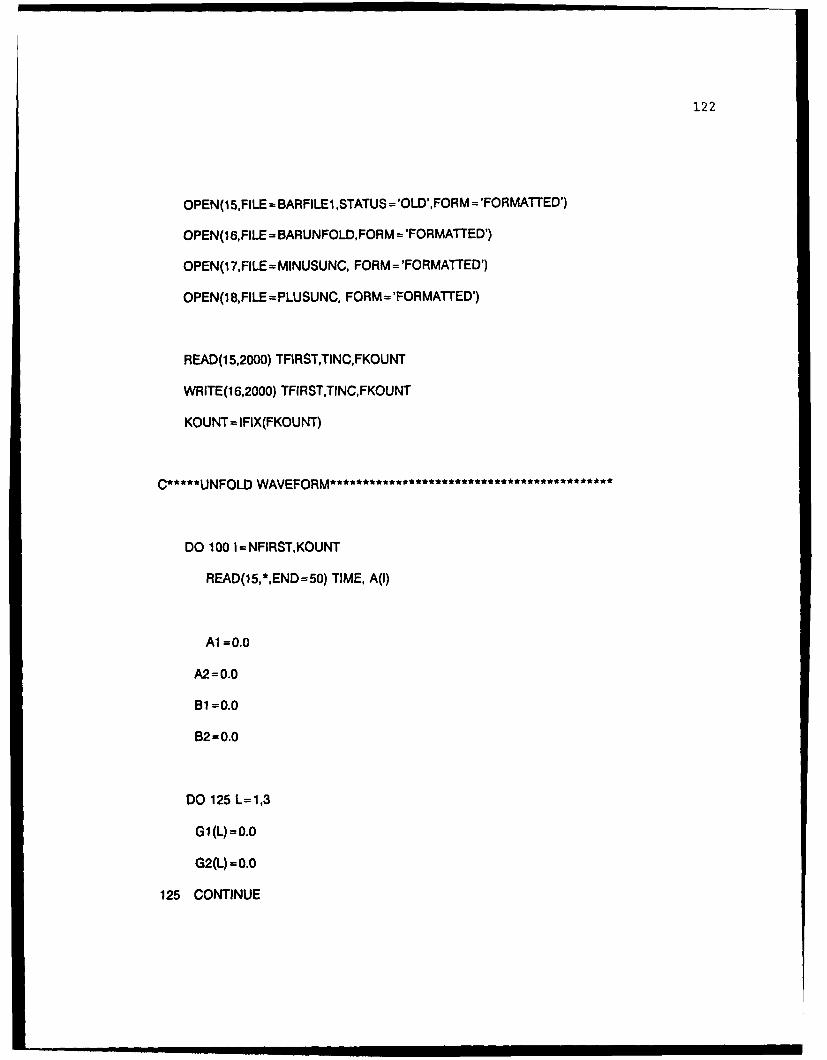
122
OPEN(l 5,FILE = BARFILEl ,STATUS ='OLD',FORM ='FORMATTED')
OPEN(16,FILE=BARUNFOLDFORM ='FORMATTED')
OPEN (1 7,FILE= MINUSUNO, FORM = 'FORMATTED')
OPEN(1 8,FILE=PLUSUNO, FORM ='FORMATTED')
READ(1 5,2000) TFIRST,TINC,FKOUNT
WRITE(1 6,2000) TFIRST,TINC,FKOUNT
KOUNT=IFIX(FKOU NT)
C*****UNFOLD WAVEFORM****************************************~**
DO 100 I= NFIRST,KOUNT
READ(15,*,END=50) TIME, A(I)
Al =0.0
A2 =0.0
Bl =0.0
B2=0.0
DO 125 L =1,3
Gi (L) =0.0
G2(L) = 0.0
125 CONTINUE

123
DO 150 K1 = 1,3
IF (Kl.EQ.1) THEN
Cl =C-UC
ELSE IF (K1.EQ.2) THEN
Cl =C
ELSE IF (KI.EQ.3) THEN
C1 =C+UC
ENDIF
C*****IF "1" LIES PRIOR TO FIRST TENSILE REFLECTION, WRITE******
C***** POINT DIRECTLY TO OUTPUT F****************************
TWOC=2./Cl
IF (TIME.LT.(TOA+TWOC*(BARLEN-X))) THEN
GO TO 5
ELSE
C*****IF "1" LIES AFTER FIRST TENSILE REFLECTION, FIND**********
C*****OUT WHICH REFLECTION IT UES IN, AND SET VARIABLE "N*****
C*****TO THAT NUMBER*******************************************
DIF= (TIME-(TOA+TWOC*(BARLEN-X)))/(TWOC*BARLEN)
WNUM =AINT(DIF)
DEC= DIF-WNUM
IF (DEC.LT.0.50) THEN

124
DIF= DIF+ 0.50
ENDIF
N==NINT(DIF)
ENDIF
C*****PERFORM SUMMATIONS OF SECOND TERM*************************
DO 200 K=l,N
TEMP =(2./Cl )*(FLOAT(K)*BARLEN-X)
J -IFIX(TEMP/TI NC)
J=I-J
G I (Ki) =Gi (Kl) + (GAMMAl **K) *(GAMMA2**(K-1l))*F(J)
IF(Kl .EQ.2) THEN
Al = Al + K*(GAMMAI **(K-1)) *(GAMMA2**(K-1))*F(J)
Bl =Bl + (K-l)*(GAMMAl**K)*(GAMMA2**(K-2))*F(J)
ENDIF
C*****DETERMINE IF SUMMATIONS OF THIRD TERM ARE NECESSARY,
C.*****AND IF SO, PERFORM TE*****************
TEMP = (2./C1)*FLOAT(K)*BARLEN
VAL2 =TIME-TEMP-TOA
IF(VAL2.GT.0) THEN
J =IFIX(TEMP/TINC)
J =I-J
G2(Kl) = G2(Kl) + (GAMMAl **K)*(GAMMA2**K)*F(J)

125
IF(K1.EQ.2) THEN
A2 =A2 +K*(GAMMA1 **(K.1 ))*(GAMMA2**K)*F(J)
B2= 62 +K*(GAMMA1 **K)*(GAMMA2**(K.1 ))*F(J)
END IF
END IF
200 CONTINUE
150 CONTINUE
C*****COMPUTE AMPUITUDE OF UNFOLDED VALUE OF POINT 1" AND
C*****WRITE IT TO THE OUTPUTFLE***************
5 F(I) =A(I) + Gi (2)-G2(2)
FMINUS =F(I)-(A(I) + GI (1 )-G2(1))
FPLUS = F(I)-(A(I) + Gi (3)-G2(3))
UNCA= (Al .A2)*UA
UNCB= (B1-B2)*UB
UP = F(I)-FPLUS + ((UNCA**2) + (UNCB**2))**0.5
UM = F(i)-FMINUS.((UNCA**2) + (UNCB**2))**0.5
WRITE(16,4000) TIME, F(I)
WRITE(17,4000) TIME, UIM
WRITE(18,4000) TIME, UP
100 CONTINUE
50 CLOSE (UNIT= 15)
CLOSE (UNIT= 16)
CLOSE (UNIT= 17)

126
CLOSE (UNIT= 18)
C*****FORMAT STATEMENTS*****************************************
1000 FORMAT(A30)
2000 FORMAT(E12.4,/,E12.4,/,E12.4)
3000 FORMAT(E12.4)
4000 FORMAT(F1O.8,1X,F12.5)
END
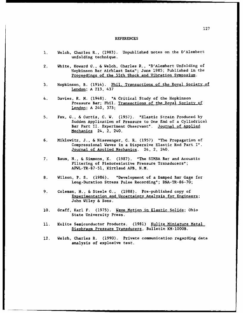
127
REFERENCES
1. Welch, Charles R., (1983). Unpublished notes on the D'Alembertunfolding technique.
2. White, Howard G., & Welch, Charles R., "D'Alembert Unfolding ofHopkinson Bar Airblast Data"; June 1985; Published in theProceedings of the 55th Shock and Vibration Symposium.
3. Hopkinson, B. (1914). Phil. Transactions of the Royal Society ofLondon; A 213, 437
4. Davies, R. M. (1948). "A Critical Study of the HopkinsonPressure Bar; Phil. Transactions of the Royal Society ofLondon; A 240, 375;
5. Fox, G., & Curtis, C. W. (1957). "Elastic Strain Produced bySudden Application of Pressure to One End of a CylindricalBar Part II. Experiment Observant". Journal of AppliedMechanics 24, 2, 240.
6. Miklowitz, J., & Nisewanger, C. R. (1957) "The Propagation ofCompressional Waves in a Dispersive Elastic Rod Part I".Journal of Applied Mechanics. 24, 2, 240.
7. Baum, N., & Simmons, K. (1987). "The SIMBA Bar and AcousticFiltering of Piezoresistive Pressure Transducers";AFWL-TR-87-51, Kirtland AFB, N.M.
8. Wilson, P. S. (1986). "Development of a Damped Bar Gage forLong-Duration Stress Pulse Recording"; DNA-TR-86-70;
9. Coleman, H., & Steele G., (1988). Pre-published copy ofExperimentation and Uncertainty Analysis for Engineers;John Wiley & Sons.
10. Graff, Karl F. (1975). Wave Motion in Elastic Solids; OhioState University Press.
11. Kulite Semiconductor Products. (1981) Kulite Miniature MetalDiaphrazm Pressure Transducers, Bulletin KM-1000B.
12. Welch, Charles R. (1990). Private communication regarding dataanalysis of explosive test.

DISTRIBUTION LIST
Defense Nuclear Agency Ktech Corporation6801 Telegraph Road 901 Pennsylvania Ave. N.E.Alexandria, VA 22310-3398 Albuquerque, N.M. 87110
ATTN: TDTR M. Flohr ATTN: E. GaffneyATTN: SPWE K. Peterson
Logicon R & D AssociatesCommander 6940 S. Kings HwyField Command Suite 210Defense Nuclear Agency Alexandria, VA 22310Test Operations Directorate ATTN: J. WebsterKirtland AFB, NM 87115-5000
ATTN: TTST, E. Rinehart Logicon R & D AssociatesP.O. Box 9377
U.S. Army Engineer Waterways Albuquerque, NM 87119-9377Experiment Station ATTN: G. Ganong
3909 Halls Ferry RoadVicksburg, MS 39180-6199 Logicon R & D Associates
ATTN: (CEWES-SE-R) P.O. Box 92500J.K. Ingram Los Angeles, CA 90009H.G. White ATTN: C.K.B. LeeC.R. Welch
New Mexico Engineering ResearchApplied Research Associates InstituteAberdeen Research Center University of New MexicoP.O. Box 548 Albuquerque, NM 87131Aberdeen, MD 21001 ATTN: N. Baum
ATTN: N. EthridgeS-Cubed
California Research & Technology A Division of Maxwell Labs, Inc.5117 Johnson Drive P.O. Box 1620Pleasanton, CA 94588 La Jolla, CA 92038-1620
ATTN: J. Thomsen ATTN: C. Peterson
ATTN: P. ColemanCarpenter Research Corp.P.O. Box 2490 Science Applications Intl. Corp.Rolling Hills Estates, CA 90274 10260 Campus Point Drive
ATTN: H.J. Carpenter San Diego, CA 92121ATTN: C. Hsiao
Fluid Physics Inc.4265 Manchester Ave. SRI InternationalEncinitas, CA 92024 333 Ravenswood Avenue
ATTN: R. Traci Menlo Park, CA 94025-3434ATTN: D. Keough
Geo Centers, Inc.P.O. Box 428Newton Upper Falls, MA 02164
ATTN: B. Nelson

Waterways Experiment Station Cataloging-In-Publication Data
Ohrt, Alan Paul.Analysis of D'Alembert unfolding technique for Hopkinson bar gage re-
cords / by Alan Paul Ohrt ; prepared for Defense Nuclear Agency.136 p. : ill. ; 28 cm. - (Technical report ; SL-92-12)Includes bibliographic references.1. Stress waves - Measurement. 2. Physical measurements. 3.
Strain gages. I. Title. II. United States. Defense Nuclear Agency. Ill.U.S. Army Engineer Waterways Experiment Station. IV. Series: Techni-cal report (U.S. Army Engineer Waterways Experiment Station) ; SL-92-12.TA7 W34 no.SL-92-12


