
1
Hybrid Quantum Mechanics / Molecular Mechanics (QM/MM) Approaches
-Treatment of the electrostatic QM/MM interface -
Mauro Boero
Institut de Physique et Chimie des Matériaux de Strasbourg University of Strasbourg - CNRS, F-67034 Strasbourg, France
and
@Institute of Materials and Systems for Sustainability, Nagoya University - Oshiyama Group, Nagoya Japan

Treatment of the electrostatic in the QM/MM interface
- Errors in the QM/MM Interface (OECP)
- QM/MM interface: 3 level(s) coupling Hamiltonian
- MM polarization
2

From Gas-phase to complex environment
Molecules in thegas phase
Solids and liquidsgood properties reproduced using periodic boundary conditions (PBC)
-Structure (radial distributions)-Dynamics (diffusion)
Complex disordered systems
No periodicityPartitioning of the system: QM/MM
No environment
3
QM/MM Mixed Quantum-Classical
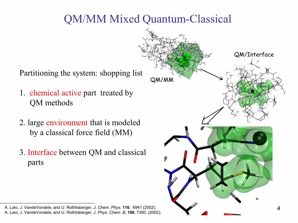
Partitioning the system: shopping list
1. chemical active part treated by QM methods
2. large environment that is modeledby a classical force field (MM)
3. Interface between QM and classicalparts
QM/MM
QM/Interface
A. Laio, J. VandeVondele, and U. Rothlisberger, J. Chem. Phys. 116, 6941 (2002); A. Laio, J. VandeVondele, and U. Rothlisberger, J. Phys. Chem. B, 106, 7300, (2002);
4

Partitioning of a QM system into 2 parts A and B: The non-linear (NL) correction
Approximations in QM/MM
QM/MM Mixed Quantum-Classical
where we use the “nuclear density”:
and are unknown.
5

QM/MM description of the subsystem B
Point charge representation of MM atoms at fix MM geometry
Because of the breakdown of the point charge representation: 2-, 3- and 4-body terms are needed:
QM/MM Mixed Quantum-Classical
Approximations in QM/MM
6

QM/MM Mixed Quantum-Classical
QM description of A & MM description of B
We collect all the approximations into the energy term
Approximations in QM/MM
7
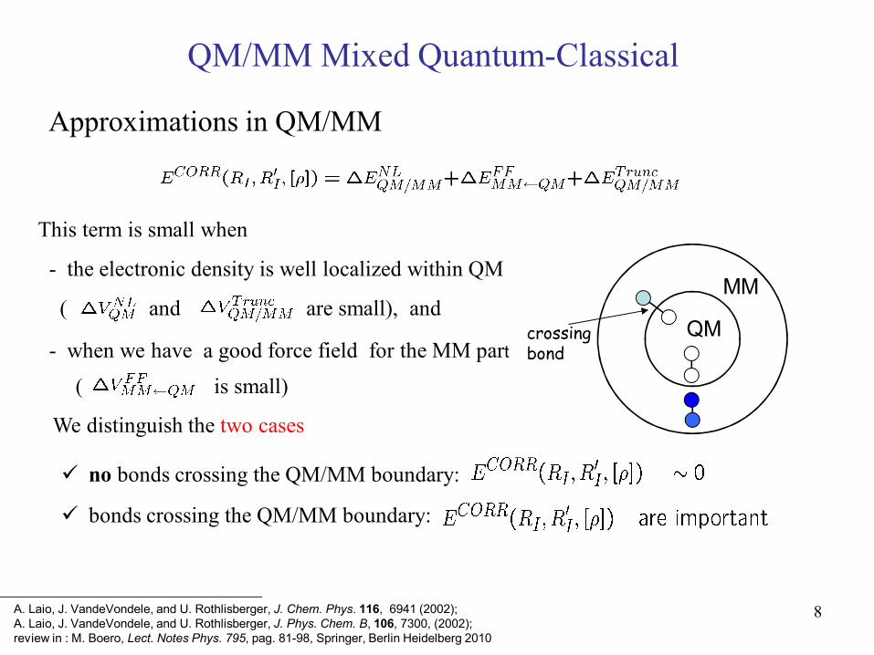
QM
MM
This term is small when
- the electronic density is well localized within QM
( and are small), and
- when we have a good force field for the MM part
no bonds crossing the QM/MM boundary:
bonds crossing the QM/MM boundary:
crossingbond
QM/MM Mixed Quantum-Classical
We distinguish the two cases
( is small)
A. Laio, J. VandeVondele, and U. Rothlisberger, J. Chem. Phys. 116, 6941 (2002); A. Laio, J. VandeVondele, and U. Rothlisberger, J. Phys. Chem. B, 106, 7300, (2002);review in : M. Boero, Lect. Notes Phys. 795, pag. 81-98, Springer, Berlin Heidelberg 2010
Approximations in QM/MM
8
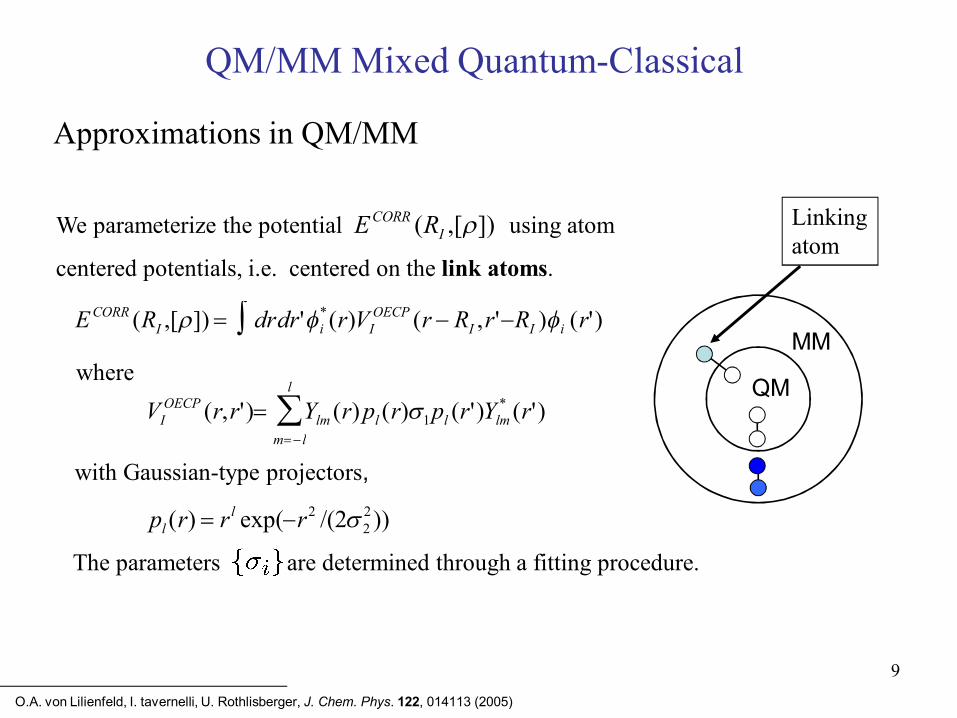
We parameterize the potential using atom
centered potentials, i.e. centered on the link atoms.
QM/MM Mixed Quantum-Classical
with Gaussian-type projectors,
QM
MMwhere
Linkingatom
The parameters are determined through a fitting procedure.
E CORR (RI ,[]) drdr'i* (r)VI
OECP (r RI ,r'RI )i (r')
VIOECP (r,r') Ylm (r) pl (r)1
m l
l
pl (r')Ylm* (r')
pl (r) r l exp(r2 /(2 22))
ECORR (RI ,[])
O.A. von Lilienfeld, I. tavernelli, U. Rothlisberger, J. Chem. Phys. 122, 014113 (2005)
9
Approximations in QM/MM

According to the Hohenberg-Kohn theorem
QM/MM Mixed Quantum-Classical
QM
MM
“ the external potential is determined, within a trivial additive constant , by the electron density .This also determines the ground state wave function and all other electronic properties of the system”
In our QM/MM scheme we optimize the parameters of the atom-centered potential in order to better reproduce the real quantum density in the QM volume (obtained using a full QM description of the total system). Thus we minimize the penalty function:
O.A. von Lilienfeld, J. Chem. Phys. 122, 014113 (2005)
Approximations in QM/MM
10
Linkingatom
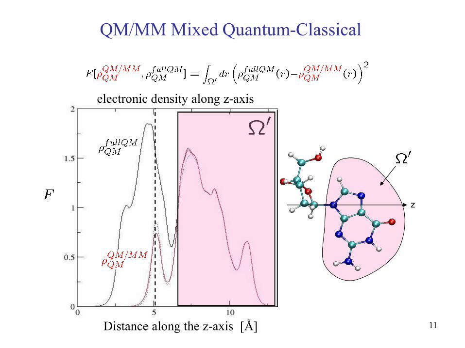
electronic density along z-axis
Distance along the z-axis [Å]
z
QM/MM Mixed Quantum-Classical
11

HOOC1-CH3
HOOC1-Dconv
(1V)
HOOC1-Dopt
(DCACP)
ESP (CH3/D) ESP (C1)Dipole [D]
1.67
2.87
1.41
0.00[-0.30 + 3*0.1]
0.32
- 0.03
0.74
0.28
0.54
Example: Acetic acid (Box size: 8 Å, gas phase, 80 Ry PW cutoff)
HO
O
H
HH
DO
O
H
QM/MM Mixed Quantum-Classical
O.A. von Lilienfeld, I. tavernelli, U. Rothlisberger, J. Chem. Phys. 122, 014113 (2005)
Approximations in QM/MM
12

H tot[{i(ri)},{RI }] H DFT [{i(ri)};{RI }] H int[{i(ri)},{R I}] H MM [{RI }]
QM/MM Hamiltonian coupling additive scheme(just a reminder)
13

QM/MM Hamiltonian coupling: Additive scheme
Scaling in a (not only) plane wave implementation:
H tot[{i(ri)},{RI }] H DFT [{i(ri)};{RI }] H int[{i(ri)},{R I}] H MM [{RI }]
H DFT [{i(ri)};{RI }] : QM-part: Hartree and xc interaction O(Nel NG NG )
H int [{i(ri)},{R I}] : QM/MM interface O(N cl NG )
H MM [{RI }] : MM part: classical (ff) potential O(N cl N cl )
atoms classical ofnumber theis functionsset -basisor wavesplane ofnumber theis
cl
G
NN
14

H int (r),{qI ,RI } qII 1
Ncl
d3r (r)r RI
Interaction Hamiltonian
Potential acting on the QM electronic density
Forces acting on the MM charged atoms:
E int[(r),{qI ,RI }](r)
qI
r RII 1
Ncl
V int (r)
int3
3int )(
}],{),([
III
II
II FRrRrrrdq
RRqrE
QM/MM Hamiltonian coupling: Electrostatics
15

H int (r),{qI ,RI } qII1
Ncl
d3r (r)r RI
The nested sums (over the classical MM atoms and over the discretized QM volume) are in general computationally very expensive
Ncl can be of the order of 100'000 - 500'000Ngrid can be of the order of 200 200 200
QM/MM Hamiltonian coupling: Electrostatics
16
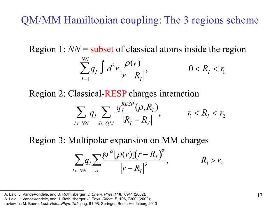
QM/MM Hamiltonian coupling: The 3 regions scheme
Region 1: NN = subset of classical atoms inside the region
Region 2: Classical-RESP charges interaction
Region 3: Multipolar expansion on MM charges
qIqJ
RESP (,RI )RI RJJQM
I NN , r1 RI r2
qII NN [(r)] r RI
r RI3
, RI r2
qII1
NN
d 3r (r)r RI
, 0 RI r1
A. Laio, J. VandeVondele, and U. Rothlisberger, J. Chem. Phys. 116, 6941 (2002); A. Laio, J. VandeVondele, and U. Rothlisberger, J. Phys. Chem. B, 106, 7300, (2002);review in : M. Boero, Lect. Notes Phys. 795, pag. 81-98, Springer, Berlin Heidelberg 2010
17

Generally we test:
However in all the known cases it isr1 ~ 10-12 a.u. r2 ~ 20-25 a.u.
Only NN < MMatoms in this shell
Divide the world in 3 domains:1) Close to the QM region (r < r1)2) Not too far, i.e. ESP region (r1 < r < r2)3) Far MM world (r > r2)
r1 r2
QM/MM Hamiltonian coupling: The 3 regions scheme
18

R1: Direct coupling – the screened Coulomb potential
QM/MM Hamiltonian couplingR1: The direct coupling
E[(r),{RI }] qIff d3r (r)
r RII NN
To avoid incompatibilities due to QM (electronic) vs. classical (point charges) description of the electrostatic, we introduce the screened Coulomb potential
E[(r ),{RI }] qIff d3r (r) v I
I NN ( r RI )
where vI (r) RcIn rn
RcIn1 rn1
is a “covalent” radius of atom I, and n is an integer (n=3)RcIn
19
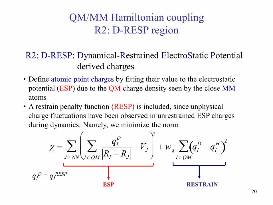
R2: D-RESP: Dynamical-Restrained ElectroStatic Potential derived charges
• Define atomic point charges by fitting their value to the electrostatic potential (ESP) due to the QM charge density seen by the close MMatoms
• A restrain penalty function (RESP) is included, since unphysical charge fluctuations have been observed in unrestrained ESP charges during dynamics. Namely, we minimize the norm
qI
D
RI RJ
VJI QM
J NN
2
wq qID qI
H I QM 2
ESP RESTRAINqI
D = qIRESP
QM/MM Hamiltonian couplingR2: D-RESP region
20

qI
D
RI RJ
VJI QM
J NN
2
wq qID qI
H I QM 2
is minimized on the fly during the dynamics.wq = weight parameter to reduce charge fluctuations:
VJ d 3r(r) u r RJ
The potential VJ is the Coulomb potential generated on the MM atom J by the electronic density distribution
25.010.0 qw
where u(|r - rJ|) is a Coulomb potential modified at short range to avoid spurious over-polarization effects.
QM/MM Hamiltonian couplingR2: D-RESP region
21

22
Hirshfeld charges ?
wq qID qI
H I QMIn the restrain term
qIH are the so-called Hirshfeld charges. They are defined as
qIH d3r r
Iat r RI K
at r RK K
ZI
where at is the atomic (pseudo) valence charge density andZI d3rat r RI
is the bare valence charge of the I-th atom.
QM/MM Hamiltonian couplingR2: D-RESP region
F. L. Hirshfeld, Theoret. Chim. Acta,44, 129-138 (1977)
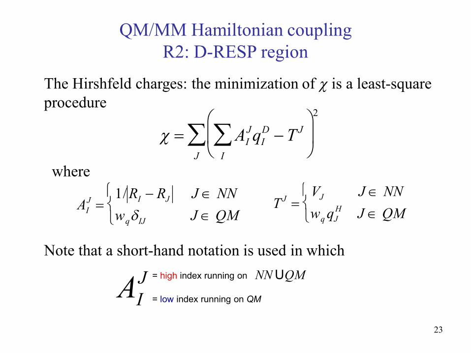
AIJqI
D T J
I
J
2
AIJ
1/ RI RJ J NNwqIJ J QM
T J VJ J NNwq qJ
H J QM
Note that a short-hand notation is used in which
AIJ = high index running on
= low index running on QM
NN UQM
The Hirshfeld charges: the minimization of is a least-square procedure
where
23
QM/MM Hamiltonian couplingR2: D-RESP region

The Hirshfeld charges least-square procedure:
qI
D 0 AKJ qK
D T J
K
J AI
J 0
and the (analytical) solution is trivially
qID HIK
1 tKK
where andHIK AIJ AK
J
J tK AK
J T J
J
QM/MM Hamiltonian couplingR2: D-RESP region
24

VJRESP[(r)] qI
D[(r)]RI RJI QM
VJDFT [(r)] d3r(r) u r RJ
The D-RESP potential
vRESP (r) E RESP
(r)
E RESP
qID
I QM qI
D
(r)
while the (extra) forces on the atoms are
FJ rJE RESP
E RESP
RJ
E RESP
qID
I QM qI
D
RJ
D-RESP potential - summary
can be computed in a much more efficient way than the exact DFT potential
The corresponding potential on the electrons becomes
QM/MM Hamiltonian couplingR2: D-RESP region
25
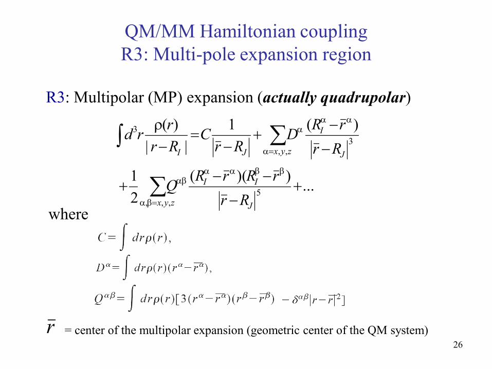
= center of the multipolar expansion (geometric center of the QM system)
R3: Multipolar (MP) expansion (actually quadrupolar)
where
...))((21
)(1||
)(
5,,,
3,,
3
J
II
zyx
J
I
zyxJI
RrrRrRQ
RrrRD
RrC
Rrrrd
r
QM/MM Hamiltonian couplingR3: Multi-pole expansion region
26

QM/MM Hamiltonian couplingSummary: R1 + R2 + R3
EQM / MM [(r),{RI }] qIff d 3r (r) vI (r RI )
I NN
qI
D[(r)]qJ
RI RJI QM
JMM (ESP )
C qJ
RI RJJMM(MP) D
x,y,z qJ
r RJ3
JMM(MP) (RI
r )
Q
,x,y,z qJ
r RJ5
JMM(MP) (RI
r )(RI r ) ...
R1
R2
R3
27

&QMMM COORDINATESINPUTTOPOLOGYADD HYDROGENAMBERARRAYSIZES ... END ARRAYSIZESBOX TOLERANCEBOX WALLSCAPPINGCAP HYDROGENELECTROSTATIC COUPLING [LONG RANGE]ESPWEIGHTEXCLUSION fGROMOS,LISTgFLEXIBLE WATER [ALL,BONDTYPE]FORCEMATCH ... END FORCEMATCHGROMOS
HIRSHFELD [ON,OFF]MAXNNNOSPLITRCUT NNRCUT MIXRCUT ESPRESTART TRAJECTORYSAMPLE INTERACTING [OFF,DCD]SPLITTIMINGSUPDATE LISTVERBOSEWRITE LOCALTEMP [STEP fn ltg]
&END
QM/MM Hamiltonian couplingInput file
28

QM/MM Hamiltonian couplingInput file
ELECTROSTATIC COUPLING [LONG RANGE]Section: &QMMM The electrostatic interaction of the quantum system with the classical system is explicitly kept
into account for all classical atoms at a distance R ≤ RCUT_NN from any quantum atom and for all the MM atoms at a distance of RCUT_NN < r ≤ RCUT_MIX and a charge larger than 0.1e (NN atoms).
MM-atoms with a charge smaller than 0.1e and a distance of RCUT_NN <r ≤ RCUT_MIX and all MM-atoms with RCUT MIX < r ≤ RCUT ESP are coupled to the QM system by a ESP coupling Hamiltonian (EC atoms).
If the additional LONG RANGE keyword is specified, the interaction of the QM-system with the rest of the classical atoms is explicitly kept into account via interacting with a multipoleexpansion for the QM-system up to quadrupolar order. A file named MULTIPOLE is produced.
If LONG RANGE is omitted the quantum system is coupled to the classical atoms not in the NN-area and in the EC-area list via the force-field charges.
If the keyword ELECTROSTATIC COUPLING is omitted, all classical atoms are coupled to the quantum system by the force-field charges (mechanical coupling). The files INTERACTING.pdb, TRAJECTORY_INTERACTING, MOVIE_INTERACTING, TRAJ_INT.dcd, and ESP (or some of them) are created. The list of NN and EC atoms is updated every 100 MD steps. This can be changed using the keyword UPDATE LIST.
The default values for the cut-offs are RCU_ NN=RCUT_MIX=RCUT_ESP=10 a.u..These values can be changed by the keywords RCUT_NN, RCUT_MIX, and RCUT_ESP withrnn ≤ rmix ≤ resp.
29

The Redistributed Charge scheme (RC) is a scheme to improve the electrostatic at the linking atom.
Y. Zhang, H. Lin and D. G. Truhlar, J. Chem. Theory Comput. 3, 1378-1398 (2007)
QM/MM Hamiltonian couplingThe Redistributed Charge scheme (RC)
It tunes the electrostatic balance between quantum and classical description at the interface.
30

QM/MM Hamiltonian couplingThe Redistributed Charge scheme (RC)
The RC scheme is used in conjunction with hydrogen capping approach
Nomenclature for the MM atoms:
M1
M2x
M2y
M2z
M3
M3
M3
Q1
Q2x
Q2y
Q2z
Q3
Q3
Q3
31

QM/MM Hamiltonian couplingThe Redistributed Charge scheme (RC)
The RC scheme is used in conjunction with hydrogen capping approach
The MM partial charge of atom M1 is redistributed evenly over 3 point charges q0=qM1/n, where n is the number of M1-M2 bonds.
The capping hydrogen (or linking atom, HL) carries no charge.
Location of the charges q0:
H. Lin and D. G. Truhlar, Theor. Chem. Acc. 117, 185-199
RM 1 Rq0
RM 1 RM 2
Cq0 0.5
32

QM/MM Hamiltonian couplingThe Redistributed Charge and Dipoles scheme (RCD)
The RC method introduces an error in the M1-M2 dipole.
The dipole q0R (R=|RM1-RM2|) reduces by a factor of (1 – Cq0).For Cq0 = 0.5, the contribution reduces by 50%.
In the RCD method, the values of redistributed charges q0 and of the charges on M2 atoms (labeled k = 1, 2, …) are further modified such that these contributions to the M1−M2 bond dipoles are preserved.
0
0
011
0,2,2
00
q
qkM
RCDkM
q
RCD
CCq
qqC
33
QM/MM Hamiltonian couplingThe Polarized-Boundary method (RCPB/RCDPB)
In the RC and RCD schemes, the QM subsystem is polarized by the MM system, but the MM subsystem is not polarized by the QM subsystem, resulting in an unbalanced treatment of the electrostatic interactions between the QM and MM subsystems.
The polarized boundary RC (PBRC) and polarized-boundary RCD (PBRCD) schemes make improvements in this regard to the RC and RCD schemes, respectively, by allowing self-consistent mutual polarizations between the QM and MM subsystems near the boundary.
In the PBRC and PBRCD schemes, the polarization of the MM subsystem due to the QM electrostatic potential is accomplished by adjusting the MMatomic partial charges in the QM/MM calculations according to the principles of electronegativity equalization and charge conservations.
34

QM/MM Hamiltonian couplingThe Polarized-Boundary method (RCPB/RCDPB)
First, the MM atomic partial charges are assigned to the MM atoms, and the QM/MM calculation is performed.
The electric field generated by the QM subsystem (nucleiand electronic wavefunctions) is computed and imposed on the MM, and a new set of MM atomic partial charges is determined according to the electronegativity equalization and charge conservation.
The new set of partial charges replaces the old set of partial charges, and a new QM/MM calculation is performed with the updated partial charges (new external potential for the DFT calculation).
convergence ?
STOP
Convergence= until the variations in partial charges are smaller than preset thresholds, or until the number of iterations exceeds a preset value.
no
yes
35

QM/MM Hamiltonian couplingThe Polarized-Boundary method (RCPB/RCDPB)
Charge equalization method by Rappé and Goddard.[A. K. Rappé and w. A. Goddard, W. A. (1991) J. Phys. Chem. 95, 3358-3363 (1991).]
EQ (Q1,Q2,...,QNcl) (E I 0 I
0QI 12
QI2JII
0 )I
12
QII J QJ JIJ QI d3r (r)
r RI
I
E I 0 is the unperturbed reference charge
I0 = E
Q
I0
=1/2(IP - EA) is the first order response (electronegativity)
term)Coulomb-self (repulsive responseorder second theis EA)-(IP=QE=
I02
20
IIJ
JIJ0 Coulomb interaction between unit charges at I and J (at disrance R =| RI - RJ |)
Consider the classical energy expression:
36

QM/MM Hamiltonian couplingThe Polarized-Boundary method (RCPB/RCDPB)
The charge equalization method is based on the minimization of the energy EQ (Q1,Q2,...,QNcl
)i.e.
under the constraints
0),...,,( 0021
IJ
JIJJIIII
NI QJQJQEQQQ
cl
1. 1 2 K Ncl
2. Qtot QII1
Ncl
This leads to a linear system of equations CD Dwhere D1 Qtot, Di i
0 10 for i 2
C1i Qi, Cij Jij J1 j for i 2
37

QM/MM Hamiltonian couplingThe Polarized-Boundary method (RCPB/RCDPB)
Electronegativity equalization method by Mortier et. al.[W. J. Mortier, S. K. Ghosh, and S. Shankar, J. Am. Chem. Soc. 108, 4315- 4320 (1986) .]
The existence of a unique chemical potential everywhere in the molecule establishes the electronegativity equalization principle that Mortier write as
I (Q1,Q2,...,QNcl) ( I
0 I ) 2(I0 I )QI
QJ
RIJJI
clN 21with
and are the neutral atom electronegativity and hardness, respectively, QI, and QJ are the charges on atoms I and J, and RIJ, is the internuclear distance. The parameters and are the corrections to the neutral atom electronegativity and hardness that arise as a consequence of bonding.
I0 I
0
I I
38

QM/MM Hamiltonian couplingThe Polarized-Boundary method (RCPB/RCDPB)
and are obtained by calibrating through small-molecule calculations and are transferable and consistently usable for calculating charges in any molecule.
I I
39


