
Human Capital and Economic Opportunity: A Global Working Group
Working Paper Series
Human Capital and Economic Opportunity Working GroupEconomic Research CenterUniversity of Chicago1126 E. 59th StreetChicago IL [email protected]
Working Paper No.
Early life adversity and children’s competence development:
evidence from the Mannheim Study of Children at Risk
Dorothea Blomeyer*, Katja Coneus**, Manfred Laucht*, Friedhelm Pfeiffer***
* Central Institute of Mental Health (ZI), Mannheim ** SAP, Walldorf
*** Centre for European Economic Research (ZEW), Mannheim
October 15, 2012
This paper investigates the role of early life adversity and home resources in terms of
competence formation and school achievement based on data from an epidemiological
cohort study following 364 children from birth to adolescence. Results indicate that
organic and psychosocial risks present in early life as well as the socio-emotional home
environment are significant predictors for the formation of competencies. Competencies
acquired at preschool age predict achievement at school age. A counterfactual analysis
is performed to assess trade-offs in the timing of interventions in the early life cycle.
Keywords: Initial Risk Matrix, Socio-Emotional and Economic Home Resources, Intel-ligence, Persistence, Peer Relationship, School Achievement JEL-Classification: D87, I12, I21, J13 Acknowledgements: We gratefully acknowledge generous support from the Leibniz Association (LA), Bonn, through the grant “Non-cognitive Skills: Acquisition and Economic Consequences”. Dorothea Blomeyer and Manfred Laucht thank the German Research Foundation (DFG9 and the Federal Ministry of Education and Research (BMBF) for their support in conducting the Mannheim Study of Children at Risk. The views expressed in this article are those of the authors and do not necessarily reflect the views of the LA, the BMBF or the DFG. For helpful discussions, we thank Anja Achtziger, Lex Borghans, Liam Delaney, Bart Golsteyn, James Heckman, Winfried Pohlmeier, Petra Todd, the editor of the Journal of Economics and Statistics and two referees. For competent research assis-tance, we are grateful to Marianella Gonzalez, Moritz Meyer and Julia Schäfer. All opinions and mistakes are our own. Corresponding author: Friedhelm Pfeiffer, Centre for European Economic Research (ZEW), P.O. Box 103443, D-68034 Mannheim. Tel.: +49-621-1235-150, E-mail: [email protected]
1
1. Introduction
Competencies are formed in a dynamic and cumulative process between adult caregiv-
ers and children through a series of development transitions. There is a burgeoning eco-
nomic literature using psychological data from infancy to understand the role of the
initial risk matrix and early home environment for later development (Blomeyer et al.,
2009, Cunha et al., 2010, Currie, 2011, Heckman, 2007, Pfeiffer and Reuß, 2008, Spieß,
2011, among others).
We contribute to this multidisciplinary research by employing unique data from a de-
velopmental psychological approach, the Mannheim Study of Children at Risk, abbr.
MARS (derived from the German title of the study: “Mannheimer Risikokinder Stud-
ie”). MARS is an epidemiological cohort study that follows a carefully selected group
of children from birth to adulthood. Children at risk are oversampled in the data. This is
an advantage for our purpose since the total sample covers the full range of early life
adversity stemming from the initial risk matrix, be it organic or psychosocial in nature
(see Blomeyer et al., 2009, Coneus et al., 2012, Laucht et al., 2004). In addition, the
data contain a unique set of psychological expert ratings on stage-specific competencies
and the home environment in significant stages of development.1 This peerless data
feature improves the chance to uncover the key role of early interaction for human capi-
tal formation.
The contribution to the literature is an initial assessment of trade-offs in the timing of
interventions at different development stages to foster social achievement. We extend
our previous work in three further directions. First, the socio-emotional home environ-
1 Infancy, toddlerhood, preschool age, elementary school age, secondary school age.
2
ment is measured with the wide-spread original Home Observatory for Measurement of
the Environment (HOME) (Caldwell and Bradley, 1984) for the first time. The findings
are compared with our previous study, Blomeyer et al. (2009), where a modified version
of the HOME was utilized, enriched with information on mother-child interaction dur-
ing early childhood. Second, we investigate the role of basic preschool competencies for
further social outcomes such as interests and peer relationships. Third, we elaborate on
gender differences in competence formation.
Our results demonstrate that interpersonal differences in competencies are consistently
associated with early life adversity and the socio-emotional home environment, with the
relationship being specific to age and competencies. Children are exposed to a matrix of
organic and psychosocial risks, and each factor by itself contributes to their develop-
ment as well as the sum of all factors. We conclude that advantages from beneficial so-
cio-emotional environments and disadvantages from adverse environments cumulate
during the developmental course. Thus, disadvantages in early childhood that impair
development persist and affect competence formation further during later childhood.
There is evidence for synergies and dynamic complementarities in the formation of
competencies and social outcomes. The counterfactual policy analysis suggests that
socio-emotional and economic support for disadvantaged children needs to be extended
continuously and stage-specifically.
The usage of the original instead of the modified HOME does not change these conclu-
sions. The association between the home environment and the competencies remains
significant although the estimated coefficients are slightly lower when the original
HOME is utilized. Gender seems to play no or only a moderate role in competence for-
mation over the early life cycle.
3
Our work is related to Cunha et al. (2010), who use a sample of 2,207 first-born white
children from the Children of the National Longitudinal Survey of Youth (CNLSY).
They estimate the “technology of skill formation” for two developmental stages (0 to 5
or 6, 5 or 6 to 13 or 14 years) and two competencies (cognitive, non-cognitive). Factor
models are employed to deal with the issue of measurement error in inputs and outputs,
which seem to be a serious problem in their data. In our study, we rely on the develop-
mental psychological approach and the epidemiological expert ratings and compare two
measures of the home environment. Although Cunha et al. (2010) consider only two
developmental stages and the methodology and the data differ, our results seem to be
more similar than diverse compared to their findings. Future research is needed to ex-
amine the issues related to the methods of measuring competencies and the home envi-
ronment in different data in further detail.
Our results with respect to early life adversity contribute to recent findings on long-term
outcomes of inequality at birth (see Currie, 2011), often measured with birth weight
(Black et al., 2007, among others). According to our analysis, neonatal complications,
adverse psychosocial conditions like maternal discord, low-skilled parents, overcrowd-
ing and other factors from the initial risk matrix (introduced in the next section) may
impair development of human capital in addition to birth weight.
The paper is organized as follows. Section 2 introduces the epidemiological cohort
study and the measurement of competencies and the home environment. Section 3 dis-
cusses the estimates of the stage specific technology of competence formation. In Sec-
tion 4, complementarities between basic competencies in childhood and social and aca-
demic achievement at school age are analyzed. Section 5 assesses alternative interven-
tion policies during the early life course, and Section 6 concludes.
4
2. The Mannheim Study of Children at Risk
The MARS project follows a cohort of infants to examine the impact of initial adverse
conditions on the prevalence of later developmental disorders and negative social out-
comes (Laucht et al., 1997, 2004).2 Infants were recruited from two obstetric and six
children's hospitals in the Rhine-Neckar region of Germany. Children with severe phys-
ical handicaps, obvious genetic defects or metabolic diseases were excluded. The initial
participation rate was 64.5 percent, with a slightly lower rate in families from low so-
cio-economic backgrounds. To control for confounding effects related to home re-
sources and the infant’s medical status, only first-born children with singleton births to
German-speaking parents of predominantly (> 99.0 percent) European descent, born
between February 1986 and February 1988, were enrolled.
The first 110 children were included consecutively into the study, irrespective of risk-
group status. These children form our approximate normative sample. To separate the
independent and combined effects of organic and psychosocial risks on child develop-
ment, infants were rated according to the degree of "organic" risk and the degree of
"psychosocial" risk. After the exclusion of 18 children with severe handicap 364 chil-
2 We do not investigate developmental disorders in the current study. Laucht et al. (2002, 2004) demon-strated that the negative impact of early life adversity persisted into late childhood. Rates of developmen-tal and behavioral disorders in high-risk children were up to three times higher than in non-risk children. Both organic and psychosocial risks contributed to adverse outcomes. While organic complications were related to disorders in motor and cognitive development, the detrimental effects of psychosocial adversity pertained to disorders in social-emotional functioning. The cumulative effect of early adversities was best explained by summing up the single risk effects. The SOEP mother-child questionnaires provide an addi-tional data set that follows children from birth to adolescence (see Berger et al., 2011, Spieß, 2011). As a rule, children’s competencies in these data are based on maternal assessments, not on expert ratings, with one recent exception summarized in Bartling et al. (2010) (see also Kosse and Pfeiffer, 2012). Based on experimental measures it is demonstrated that there is a positive association between mothers’ and chil-dren’s impatience.
5
dren (174 boys, 190 girls) that is 95 percent of the infants in the initial wave, remained
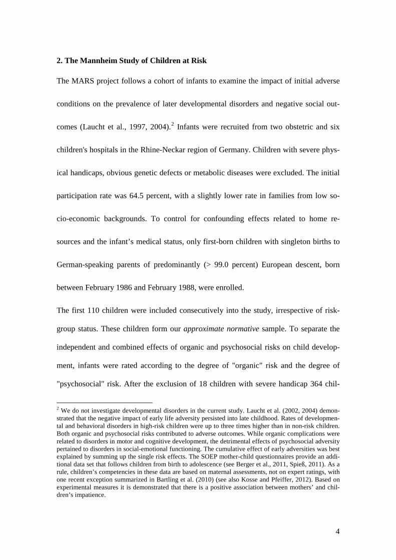
for the analysis. In the current paper, only the first five research waves are used (see
Figure 1) because the measurement of basic cognitive and motor competencies was
conducted in these waves only. These basic competencies seem to consolidate around
the age of ten years.
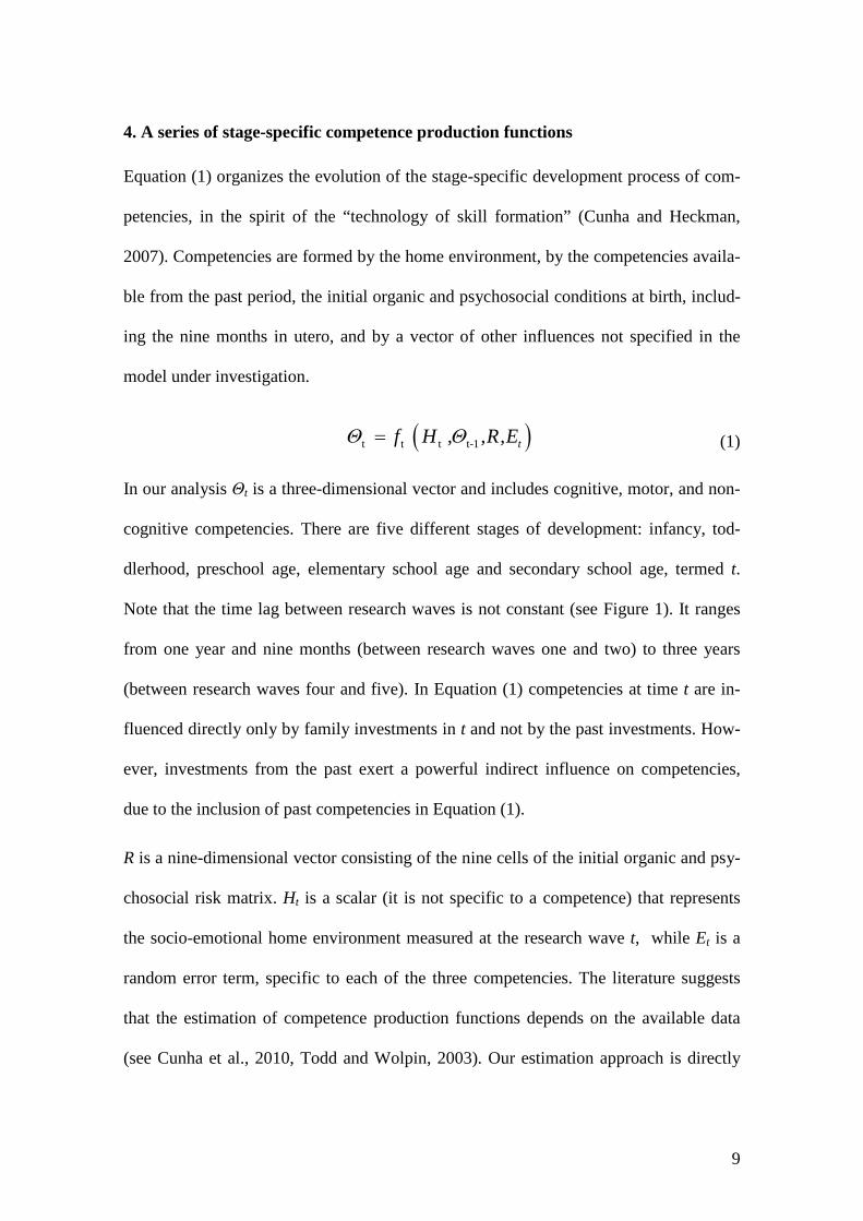
Psychometric assessments were conducted for the initial organic and psychosocial risk
matrix. Each risk factor was scaled as either non risk, moderate risk or high risk, result-
ing in a 3x3 design (Figure 1). All groups are roughly equal in size, with a slight over-
sampling in the high-risk combinations. Sex is distributed evenly in all subgroups.
Figure 1: The matrix design of the Mannheim Study of Children at Risk
Source: Laucht et al. (2004).
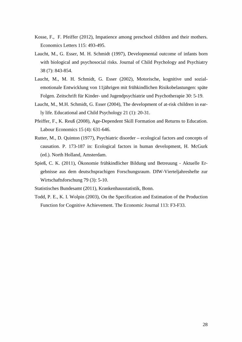
Organic risk is determined by the degree of pre-, peri- or neonatal complications. The
risk factors and their prevalence in the sample are shown in Table A1. Pre- and perinatal
variables were extracted from maternal obstetric and infant neonatal records and are
used for organic risk classification. Organic risk is classified as follows:
Risk
0 = no risk 1 = low risk 2 = high risk
1990 - 92
1986 - 88
T1
2 y
T2 4 ½ y
T3 8 y
T4 2
Research Waves 3 m
15 y Org
anic
Ris
k
1997 - 98 1994 - 96
11 y
T5
1 2
Psychosocial Risk
0
1 T6
1988 - 90
6
1. The non-risk group consists of infants who were born full-term, had normal birth
weight and no medical complications (items 1–4).
2. The moderate-risk group contains infants who had experienced premature births or
premature labor, or pre-eclampsia of the mother but no severe complications (items
5–7).
3. The high-risk group comprises infants who had very low birth weight or a clear case
of asphyxia with special care treatment or neonatal complications, such as seizures,
respiratory therapy or sepsis (items 8–10).
Psychosocial risk is determined according to a risk index proposed by Rutter and Quin-
ton (1977), which measures the presence of unfavorable family characteristics, for ex-
ample marital discord or low-skilled parents. The "enriched" family adversity index
includes eleven adverse family factors during a period of one year prior to birth, as re-
ported in Table A2. Information on the psychosocial risk rating was taken from a stand-
ardized parent interview conducted at the research wave at infancy (three months as-
sessment). Psychosocial risk is classified as follows:
1. The non-risk group includes infants who had none of the psychosocial risks.
2. The moderate-risk group contains infants with one or two of these factors.
3. The infants from the high-risk group came from a family dealing with 3 or more
of these risk factors.
Throughout this paper, the expression “competencies” summarizes basic abilities of
children, such as logical and verbal reasoning, or non-cognitive skills for instance per-
sistence. In MARS, comprehensive psychometric assessments were conducted for com-
petencies during infancy (three-month assessment), toddlerhood (two-year assessment),
7
preschool age (assessment at four and a half years), elementary school age (assessment
at the age of eight years) and secondary school age (assessment at the age of eleven
years), representing significant stages of development.
The terms cognitive, motor, and non-cognitive competencies indicate three different, yet
dependent, basic dimensions of human capability and are measured using psychometric
methods (see Blomeyer et al., 2009). Cognitive competencies include memory capacity,
information processing speed, linguistic and logic skills, and general problem-solving
abilities (IQ). Motor competencies are assessed as fine and gross motor skills and body
coordination (MQ). Our indicator of non-cognitive competencies is defined as persis-
tence (P). It measures the ability to pursue a particular activity and its continuation in
the face of distractors and obstacles.
The expression “home environment” summarizes the economic, emotional, and social
resources available for the child at home. There are two types of home environment
variables used to assess the children’s family living conditions, summarized under so-
cio-emotional home environment, H (HOME score, Bradley, 1989, Bradley et al., 2000,
Caldwell and Bradley, 1994), and one economic category, the monthly net income per
household member, Y (in real Euros, base year 1995). In comparison to our former
study (Blomeyer et al., 2009) the home environment indicates the original HOME
scales from Caldwell and Bradley (1984) without additional or enriched measures of
mother-child interaction. A comparison of econometric findings shall help to improve
our understanding of home resources and children’s outcomes.
Both measures of a child’s home resources (H and Y) decline steadily along with the
psychosocial risk dimension (Table 1). Within the group of children with high psycho-
social risk, Y is on average 67 percent of the value of the non-risk group in infancy. The
8
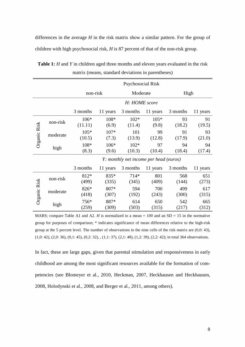
differences in the average H in the risk matrix show a similar pattern. For the group of
children with high psychosocial risk, H is 87 percent of that of the non-risk group.
Table 1: H and Y in children aged three months and eleven years evaluated in the risk
matrix (means, standard deviations in parentheses)
Psychosocial Risk
non-risk Moderate High
H: HOME score
3 months 11 years 3 months 11 years 3 months 11 years
Org
anic
Ris
k non-risk 106* (11.11)
108* (6.9)
102* (11.4)
105* (9.8)
93 (18.2)
91 (19.5)
moderate 105* (10.5)
107* (7.3)
101 (13.9)
99 (12.8)
91 (17.9)
93 (21.0)
high 108* (8.3)
106* (9.6)
102* (10.3)
97 (10.4)
94 (18.4)
94 (17.4)
Y: monthly net income per head (euros)
3 months 11 years 3 months 11 years 3 months 11 years
Org
anic
Ris
k non-risk 812* (499)
835* (335)
714* (345)
801 (409)
568 (144)
651 (273)
moderate 826* (418)
807* (307)
594 (192)
700 (243)
499 (300)
617 (315)
high 756* (259)
887* (309)
614 (503)
650 (315)
542 (217)
665 (312)
MARS; compare Table A1 and A2. H is normalized to a mean = 100 and an SD = 15 in the normative
group for purposes of comparison; * indicates significance of mean differences relative to the high-risk
group at the 5 percent level. The number of observations in the nine cells of the risk matrix are (0,0: 43),
(1,0: 42), (2,0: 36), (0,1: 45), (0,2: 32), , (1,1: 37), (2,1: 48), (1,2: 39), (2,2: 42); in total 364 observations.
In fact, these are large gaps, given that parental stimulation and responsiveness in early
childhood are among the most significant resources available for the formation of com-
petencies (see Blomeyer et al., 2010, Heckman, 2007, Heckhausen and Heckhausen,
2008, Holodynski et al., 2008, and Berger et al., 2011, among others).
9
4. A series of stage-specific competence production functions
Equation (1) organizes the evolution of the stage-specific development process of com-
petencies, in the spirit of the “technology of skill formation” (Cunha and Heckman,
2007). Competencies are formed by the home environment, by the competencies availa-
ble from the past period, the initial organic and psychosocial conditions at birth, includ-
ing the nine months in utero, and by a vector of other influences not specified in the
model under investigation.
(1)
In our analysis Θt is a three-dimensional vector and includes cognitive, motor, and non-
cognitive competencies. There are five different stages of development: infancy, tod-
dlerhood, preschool age, elementary school age and secondary school age, termed t.
Note that the time lag between research waves is not constant (see Figure 1). It ranges
from one year and nine months (between research waves one and two) to three years
(between research waves four and five). In Equation (1) competencies at time t are in-
fluenced directly only by family investments in t and not by the past investments. How-
ever, investments from the past exert a powerful indirect influence on competencies,
due to the inclusion of past competencies in Equation (1).
R is a nine-dimensional vector consisting of the nine cells of the initial organic and psy-
chosocial risk matrix. Ht is a scalar (it is not specific to a competence) that represents
the socio-emotional home environment measured at the research wave t, while Et is a
random error term, specific to each of the three competencies. The literature suggests
that the estimation of competence production functions depends on the available data
(see Cunha et al., 2010, Todd and Wolpin, 2003). Our estimation approach is directly
( )t t t t-1 tf H , ,R,EΘ Θ=

10
related to the design of our epidemiological data. The data contain comprehensive sets
of psychometric measures and expert ratings of the variables that are included in the
theoretical model.
A further assumption on the functional form is needed for performing the econometric
analysis. We assume that Equation (1) can be represented by a Cobb-Douglas function.
Taking the natural logarithm of all variables (lower case letters indicate the natural loga-
rithm), a set of three equations (2) for each research wave emerges:
(2)
where j, k, l are indices for the competencies IQ, MQ and P. i = 1, …, N is an index for
the child. r summarizes the nine cells of the two-dimensional risk matrix in MARS (in
the form of dummy variables). According to Equation (2) competencies can be pro-
duced continuously by the home environment and the stock of competencies available
from the past period. The relative contributions of ht and θt-1 in t will depend on the val-
ues of αt, the partial elasticity of the Cobb-Douglas function. While belonging to a risk
group may have lasting effects on the level of competencies, the functional form allows
that the competencies remain malleable in each period.
The Cobb-Douglas representation of competence formation has advantages and disad-
vantages. The main (and decisive) advantage arises from its flexibility and the low
number of parameters to assess the role of home resources, self-productivity, and syner-
gies in competence formation using a small data set. The main disadvantage is the as-
sumption that the elasticity of substitution between past competencies and current home
environment is one (in Cunha et al., 2010, the estimated elasticity is sometimes lower,
sometimes higher than one).
j j h, j j j k, j k l, j l jt ,i 0,t t t ,i t t 1,i t t 1,i t t 1,i t ,i* r hθ α α α θ α θ α θ ε− − −= + ⋅ + ⋅ + ⋅ + ⋅ +
11
A direct assessment of critical periods is not possible, only an indirect one. The esti-
mates are performed in each wave and the data define whether the parameters of interest
are significant, allowing indirectly investigating critical periods. For instance, if the par-
tial elasticity between the home environment and the IQ is different from zero in child-
hood (the first three research waves) but not different from zero in the last two research
waves, then one may conclude that the childhood period is a critical period for the de-
velopment of the IQ.
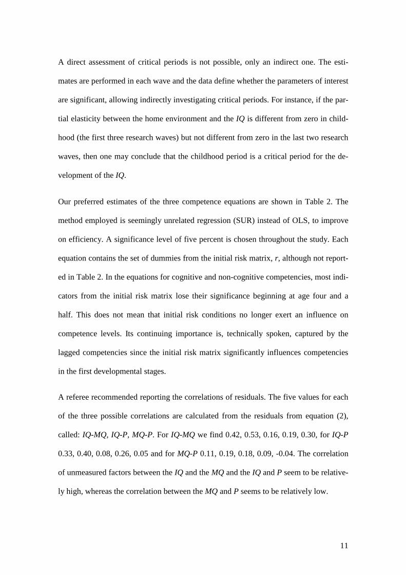
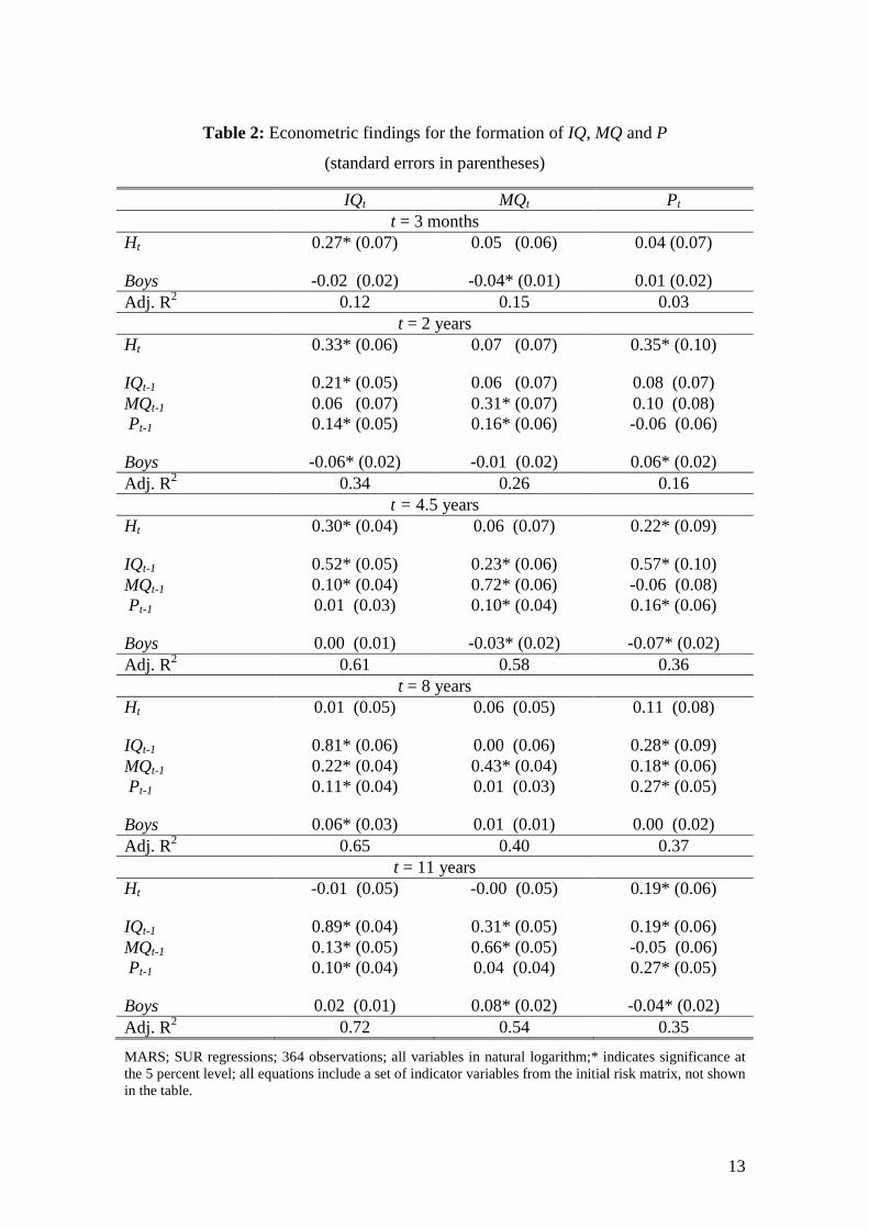
Our preferred estimates of the three competence equations are shown in Table 2. The
method employed is seemingly unrelated regression (SUR) instead of OLS, to improve
on efficiency. A significance level of five percent is chosen throughout the study. Each
equation contains the set of dummies from the initial risk matrix, r, although not report-
ed in Table 2. In the equations for cognitive and non-cognitive competencies, most indi-
cators from the initial risk matrix lose their significance beginning at age four and a
half. This does not mean that initial risk conditions no longer exert an influence on
competence levels. Its continuing importance is, technically spoken, captured by the
lagged competencies since the initial risk matrix significantly influences competencies
in the first developmental stages.
A referee recommended reporting the correlations of residuals. The five values for each
of the three possible correlations are calculated from the residuals from equation (2),
called: IQ-MQ, IQ-P, MQ-P. For IQ-MQ we find 0.42, 0.53, 0.16, 0.19, 0.30, for IQ-P
0.33, 0.40, 0.08, 0.26, 0.05 and for MQ-P 0.11, 0.19, 0.18, 0.09, -0.04. The correlation
of unmeasured factors between the IQ and the MQ and the IQ and P seem to be relative-
ly high, whereas the correlation between the MQ and P seems to be relatively low.
12
The parameter estimates in Table 2 indicate that H is positively related to cognitive and
non-cognitive competence formation at all developmental stages. However, the role of
socio-emotional home resources and the level of competencies from the past period for
competency formation changes in a way specific to age and competencies. The IQ is
positively related to H until the age of four and a half years, with an estimated partial
elasticity varying between 0.27 in infancy and 0.33 in toddlerhood. At school age, the
elasticity drops to 0.01 and is no longer significant.
P is positively associated with H at the stages of two, four and a half, and eleven years.
The partial elasticity reaches its highest value at the age of two years and is still signifi-
cant at the age of eleven. Although the partial elasticity between H and MQ is positive
(with the exception of stage eleven years), it always lacks statistical significance. There
appears to be a high degree of stability in interpersonal differences in the MQ during the
early life course. Motor abilities strongly depend on early organic and psychosocial
conditions (see Blomeyer et al., 2009) and only weakly on H during childhood.
During development, the socio-emotional home environment loses its strong relation-
ship with competencies and self- and cross-productivity increases (measured by the par-
tial elasticity of the past competencies). According to the estimates, only persistence is
associated with the socio-emotional home environment in adolescence. Although Cunha
et al. (2010) estimate a model with two broader developmental stages and do not in-
clude the MQ some of their results are comparable with ours. For instance, self-
productivity for cognitive competencies amounts to 0.487 in their first and 0.902 in their
second developmental stage (ditto p. 908, Table 1); according to our estimates, these
values are 0.52 at preschool age and 0.89 at secondary school age (Table 2), which is
nearly identical.
13
Table 2: Econometric findings for the formation of IQ, MQ and P
(standard errors in parentheses)
IQt MQt Pt t = 3 months
Ht 0.27* (0.07) 0.05 (0.06) 0.04 (0.07)
Boys -0.02 (0.02) -0.04* (0.01) 0.01 (0.02) Adj. R2 0.12 0.15 0.03
t = 2 years Ht 0.33* (0.06) 0.07 (0.07) 0.35* (0.10)
IQt-1 0.21* (0.05) 0.06 (0.07) 0.08 (0.07) MQt-1 0.06 (0.07) 0.31* (0.07) 0.10 (0.08) Pt-1 0.14* (0.05) 0.16* (0.06) -0.06 (0.06)
Boys -0.06* (0.02) -0.01 (0.02) 0.06* (0.02) Adj. R2 0.34 0.26 0.16
t = 4.5 years Ht 0.30* (0.04) 0.06 (0.07) 0.22* (0.09)
IQt-1 0.52* (0.05) 0.23* (0.06) 0.57* (0.10) MQt-1 0.10* (0.04) 0.72* (0.06) -0.06 (0.08) Pt-1 0.01 (0.03) 0.10* (0.04) 0.16* (0.06)
Boys 0.00 (0.01) -0.03* (0.02) -0.07* (0.02) Adj. R2 0.61 0.58 0.36
t = 8 years Ht 0.01 (0.05) 0.06 (0.05) 0.11 (0.08)
IQt-1 0.81* (0.06) 0.00 (0.06) 0.28* (0.09) MQt-1 0.22* (0.04) 0.43* (0.04) 0.18* (0.06) Pt-1 0.11* (0.04) 0.01 (0.03) 0.27* (0.05)
Boys 0.06* (0.03) 0.01 (0.01) 0.00 (0.02) Adj. R2 0.65 0.40 0.37
t = 11 years Ht -0.01 (0.05) -0.00 (0.05) 0.19* (0.06)
IQt-1 0.89* (0.04) 0.31* (0.05) 0.19* (0.06) MQt-1 0.13* (0.05) 0.66* (0.05) -0.05 (0.06) Pt-1 0.10* (0.04) 0.04 (0.04) 0.27* (0.05)
Boys 0.02 (0.01) 0.08* (0.02) -0.04* (0.02) Adj. R2 0.72 0.54 0.35 MARS; SUR regressions; 364 observations; all variables in natural logarithm;* indicates significance at the 5 percent level; all equations include a set of indicator variables from the initial risk matrix, not shown in the table.
14
Differences in competence formation between boys and girls seem to exist. However,
the estimated differences are stage-specific, and the positive and negative coefficients
roughly add to zero over time. In the IQ equation, the coefficient for Boys is -0.06 at the
age of two years, suggesting that boys lag 6 percent behind girls at that age. At school
age, the coefficient for Boys changes significantly and is 0.06, suggesting that boys are
ahead of girls by 6 percent. Gender-specific differences in competence development,
therefore, seem to be of only moderate importance over the early life course.
Compared to our previous study, Blomeyer et al. (2009), the estimated coefficients of
the partial elasticity of H for competencies are moderately lower in magnitude. Our
main conclusions do not change. These differences refer to the lack of scales showing
mother-child-interaction (authenticity, acceptance and reactivity in the parental behav-
iour towards the child) and language development in the original HOME, a result that
demonstrates the significant role of early mother-child interaction for development.
The relationship between family environment and children’s competencies may be re-
ciprocal. Parental responsiveness may follow complex ways. For example, parents may
try to compensate for low competencies of their child through higher H in order to sup-
port child development. Alternatively, parents may foster specifically the development
of their children with high competencies. If parents invest in such a way, then SUR es-
timates of Equation (2) may be biased.
Blomeyer et al. (2009) performed two-stage least squares (2SLS) to address this en-
dogeneity issue. The average household income per head during the first five research
waves was used as an instrument. They find higher values for the estimated coefficients
compared to OLS especially in childhood, although standard errors increased. For in-
15
stance, the elasticity of H with respect to the IQ was 2.36 (2SLS), compared to 0.55
(OLS), at three month, 1.52 (2SLS), compared to 0.38 (OLS) at two years and 0.53
(2SLS), compared to 0.38 (OLS) at 4.5 years. In later periods estimates are no longer
significant. Given that the average household income per head is a valid instrument
OLS estimates are biased downward. From our interpretation, OLS (or SUR) estimates
therefore constitute a lower bound for the parameters of interest. We will perform the
policy analysis in section 5 mainly on the basis of the OLS (or SUR) estimates in order
to compare the differences between the original H and the modified H and mention in
addition also some results from the 2SLS estimates.
4. Preschool competencies as predictors of social outcomes at school age
This section contributes to the empirical literature on dynamic complementarities during
the early life course. The association between cognitive, motor and non-cognitive com-
petencies at preschool age and popularity among peers, peer relations, the variety of
actively followed interests, interests and math grades is investigated.
Before we turn our attention to the estimates, we briefly summarize findings from the
initial risk matrix. Initial risk effects cumulate and all social adjustment scores decrease
with both dimensions of the risk matrix. The difference between the non-risk and the
high-risk groups amounts to roughly 25 percent. Math grades in the highest-risk group
are approximately one grade lower than grades in the non-risk group. A high psychoso-
cial risk is associated with the largest negative group effect. However, one exception is
worth mentioning. If there is no psychosocial risk, organic risks seem to lose their asso-
ciation with regard to interests and peers. The pursuit of interests and popularity with
peers is more affected by the initial psychosocial risk load and less by organic risks.
16
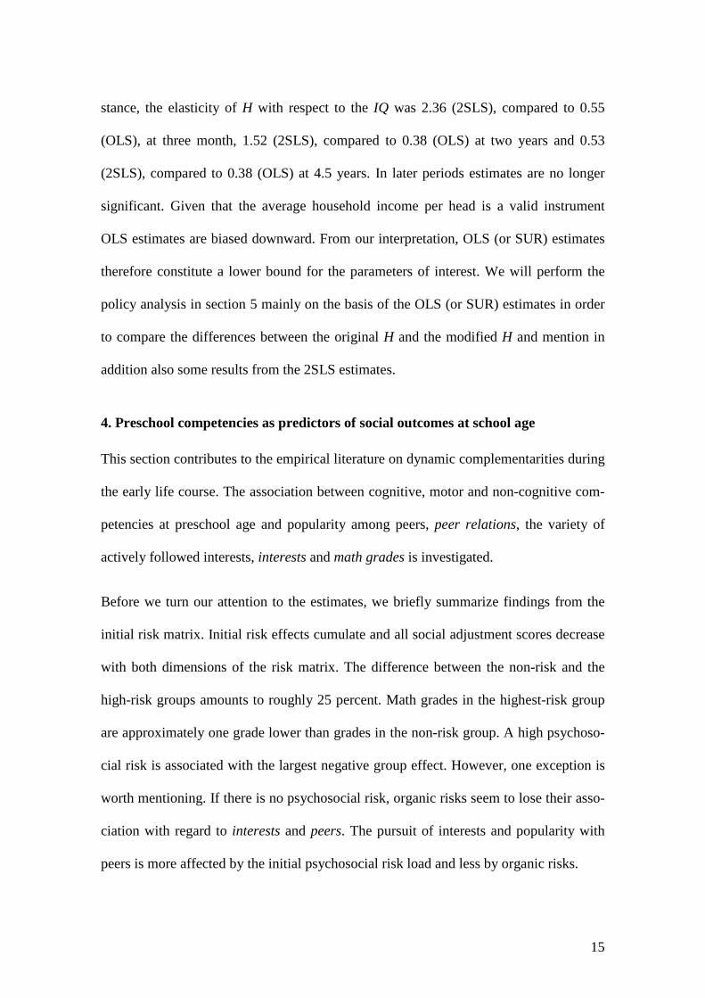
Table 3 reports findings from SUR estimates. On the right hand side, home resources,
H, and the level of IQ, MQ and P (measured at preschool age) are included. The esti-
mates can be interpreted in terms of partial elasticity, since the (natural) logarithm was
used for all variables in Table 3. Results demonstrate substantial complementarities be-
tween competencies acquired during childhood and social outcomes a child achieves at
elementary school age. Cognitive and non-cognitive competencies at preschool age pre-
dict interests at primary school age, and motor and non-cognitive abilities predict peer
relations. Contemporary H enhances popularity among peers (peer relations) and the
variety of actively followed interests (interests). Thus, children from adverse home en-
vironments seem to suffer twofold, due to poor investments in their competencies dur-
ing childhood and again due to insufficient support during school age.
Table 3: The partial elasticity of H and preschool competencies for social outcomes
at school age (eight years assessment)
interests peer relations math grades
Ht 0.55* 0.31* -0.08
IQt-1 0.45* 0.02 -0.75*
MQt-1 0.08* 0.15* -0.08
Pt-1 0.13* 0.19* -0.31*
Boy -0.02 -0.02 -0.11*
Adj. R² 0.58 0.28 0.20
N 325 325 325
MARS sample; SUR regressions; all variables in natural logarithm; social competence scores from expert ratings range from 1.0 (low), 1.1, … to 7.0 (high); grades in Germany range from 1 excellent to 6 insuffi-cient; each equation contains indicator variables for the full initial risk matrix not displayed in the table; correlation of residuals: (interests-peer relationship 0.25; interests-math grades -0.14; peer relationship-math grades -0.09). * significance at the 5 percent level.
The IQ and P measured at preschool age are significantly related to better grades in
math, while the MQ is not. Besides the IQ, P is an important predictor of achievement
17
in school, which is in line with Duckworth and Seligman (2005), among others. It is
worth mentioning that accruing to these estimates H is not related to the grades received
at age eight.
School choice in the German tracking system, as a rule, takes place after fourth grade, at
the age of ten. On average, 45 per cent of the children in the MARS attend a Gymnasi-
um at the age of 15, which is the highest-track/grammar school in Germany. In our data,
more children attend the higher-track secondary school compared to the average in Ba-
den-Wuerttemberg. The main reason is that only first-born children of German-speaking
parents are enrolled in MARS, meaning that children from immigrant families with poor
German language skills and later born children were not included in this sample. In
terms of selection to attend a grammar school, the initial risks are still important.
Among the highest-risk group, only 15 percent of the children attend the Gymnasium,
compared to 74 percent in the non-risk group. Average Gymnasium attendance decreas-
es (nearly) monotonically along the two dimensions of our risk design.
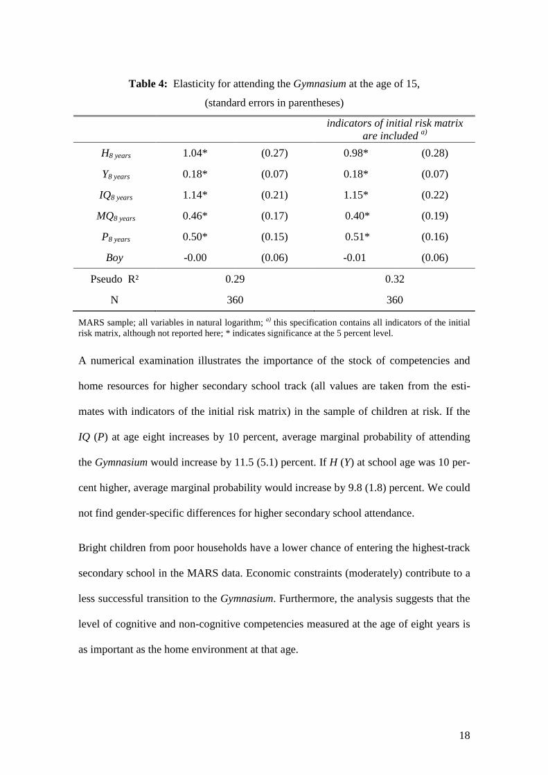
Findings from probit models predicting Gymnasium are summarized in Table 4. All
probit estimates for attending the Gymnasium include a gender dummy, the home re-
sources H and Y and the cognitive, motor and non-cognitive competencies. These are
measured at primary school age (eight years), two years before tracking takes place. In
the second specification, all indicators from the initial risk matrix are included in the
estimates. IQ, MQ and P at primary school age are significantly related to the probabil-
ity of attending the Gymnasium. The magnitude of P is lower compared to the IQ and
higher compared to the MQ. If all indicators of the initial risk matrix are included, re-
sults for the other variables do not change much. Being in the highest risk group signifi-
cantly lowers the probability of attending the Gymnasium (not displayed in the Table).
18
Table 4: Elasticity for attending the Gymnasium at the age of 15,
(standard errors in parentheses)
indicators of initial risk matrix are included a)
H8 years 1.04* (0.27) 0.98* (0.28)
Y8 years 0.18* (0.07) 0.18* (0.07)
IQ8 years 1.14* (0.21) 1.15* (0.22)
MQ8 years 0.46* (0.17) 0.40* (0.19)
P8 years 0.50* (0.15) 0.51* (0.16)
Boy -0.00 (0.06) -0.01 (0.06)
Pseudo R² 0.29 0.32
N 360 360
MARS sample; all variables in natural logarithm; a) this specification contains all indicators of the initial risk matrix, although not reported here; * indicates significance at the 5 percent level.
A numerical examination illustrates the importance of the stock of competencies and
home resources for higher secondary school track (all values are taken from the esti-
mates with indicators of the initial risk matrix) in the sample of children at risk. If the
IQ (P) at age eight increases by 10 percent, average marginal probability of attending
the Gymnasium would increase by 11.5 (5.1) percent. If H (Y) at school age was 10 per-
cent higher, average marginal probability would increase by 9.8 (1.8) percent. We could
not find gender-specific differences for higher secondary school attendance.
Bright children from poor households have a lower chance of entering the highest-track
secondary school in the MARS data. Economic constraints (moderately) contribute to a
less successful transition to the Gymnasium. Furthermore, the analysis suggests that the
level of cognitive and non-cognitive competencies measured at the age of eight years is
as important as the home environment at that age.
19
5. Policies to foster competencies and higher track school attendance
In this section, initial evidence on interventions during the early life course is provided.
The stage-specific estimates are used for assessing competency formation with counter-
factual investments based on some preliminary thought experiments. Our intention is to
highlight basic trade-offs in the timing of optimal educational policy interventions based
on the MARS data, not to make statements on interventions for a representative popula-
tion of children in Mannheim or Germany.
Assume that the government has two objectives. First, it aims at improving competen-
cies at secondary school age (eleven years) and, second, at increasing the share of chil-
dren attending the Gymnasium at the age of fifteen. The government either may help
children to overcome constraints resulting from poor socio-emotional home resources in
(early) childhood, or it may help the children later at school age through improved eco-
nomic and socio-emotional home resources, or both. Assume further that the govern-
ment is willing to raise Y by 10 percent at one or the first four developmental stages. For
the children in our sample, this would cost 66 Euros per household member per month
at the first research wave 1986/1987, and 73 Euros at the fifth research wave, 1997/1998
(real Euros, base year 1995).
If we assume that there are three household members and that it is necessary to increase
the annual (not only the monthly) income, 2.376 € would have been needed for each
household in the first research wave. The overall amount of money will depend on the
group of children selected. If ten percent of the 680 thousand (West-) German children
born in 1988 (Statistisches Bundesamt, 2011) would have been selected (68,000 house-
holds) this would have cost 161 million €, a manageable amount of money.
20
A 10-percent increase in Y has no direct implication for the formation of cognitive, mo-
tor, and non-cognitive competencies during childhood, but an indirect one. The child
will profit from an improved socio-emotional home environment, for instance from less
economic stress in the family. Parents who receive a cash transfer may have more time
to spend with their children and improve the socio-emotional home environment. When
a poor home environment has a negative impact on earnings capabilities, cash transfers
may help to overcome a vicious circle as well. For instance, research by Amarante et al.
(2011) indicates that cash transfers have the potential to improve birth outcomes; Gelber
and Isen (2012) show that public and family investments for children are complemen-
tary in nature.
In the data, a 10-percent increase in Y is partially related with a one-to-two percent in-
crease in H. This empirical relationship results from regressions of H on Y using the
log-values of Y and H, including a constant. Since we are not aware of other data to as-
sess a causal relationship between Y and H (the reason is that H is, as a rule, neither
available in official statistics nor in other survey data), in what follows the lower one-
percent finding is utilized for the following analysis.
We take all direct and indirect multiplier and accelerator effects from the stage-
dependent one-percent increase in H into account in the following way. In the first step,
a one-percent increase in H in a specific developmental stage is associated with im-
proved competencies (Table 2). In the second step, these higher competencies will in-
duce further effects in the following developmental stage through synergies in compe-
tence formation (estimated elasticity of self- and cross-productivity, Table 2). The se-
cond step is repeated for each of the remaining developmental stages.
21
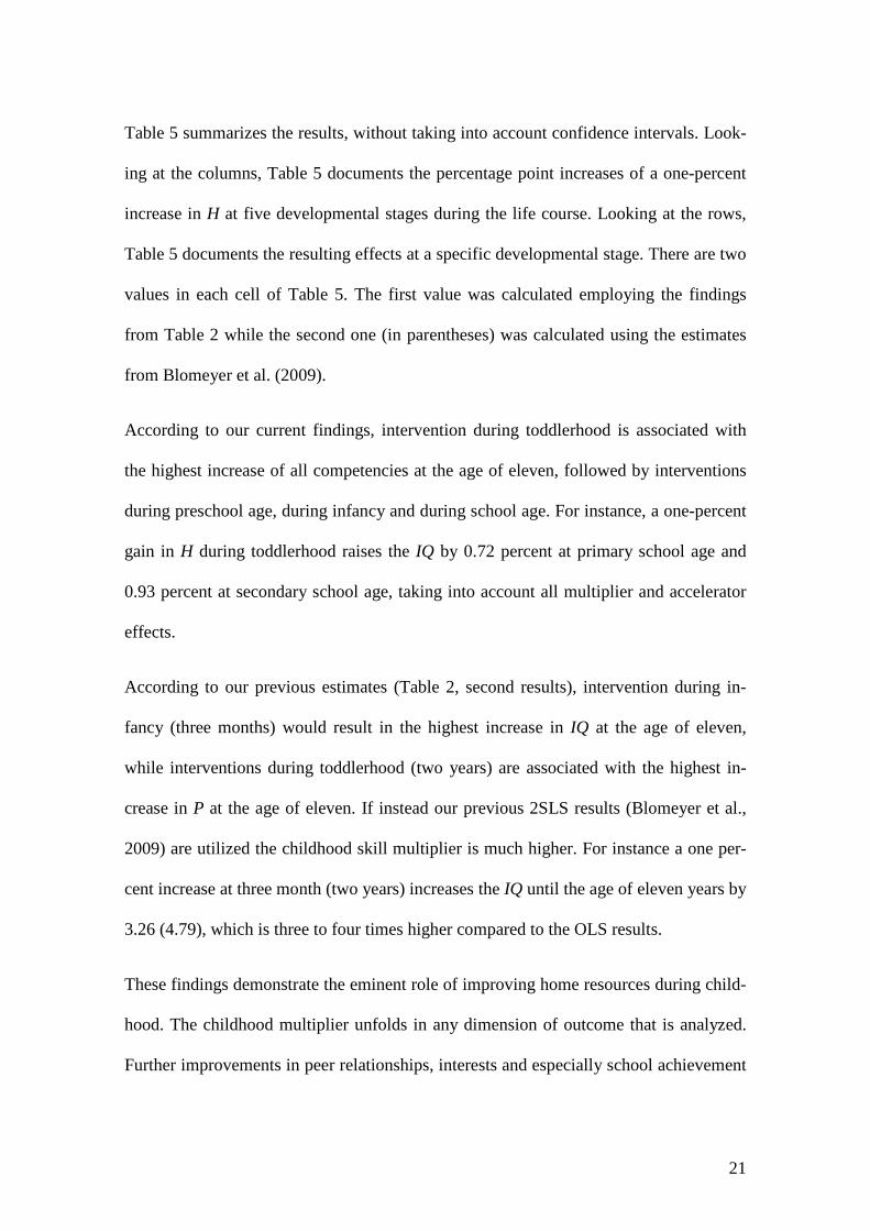
Table 5 summarizes the results, without taking into account confidence intervals. Look-
ing at the columns, Table 5 documents the percentage point increases of a one-percent
increase in H at five developmental stages during the life course. Looking at the rows,
Table 5 documents the resulting effects at a specific developmental stage. There are two
values in each cell of Table 5. The first value was calculated employing the findings
from Table 2 while the second one (in parentheses) was calculated using the estimates
from Blomeyer et al. (2009).
According to our current findings, intervention during toddlerhood is associated with
the highest increase of all competencies at the age of eleven, followed by interventions
during preschool age, during infancy and during school age. For instance, a one-percent
gain in H during toddlerhood raises the IQ by 0.72 percent at primary school age and
0.93 percent at secondary school age, taking into account all multiplier and accelerator
effects.
According to our previous estimates (Table 2, second results), intervention during in-
fancy (three months) would result in the highest increase in IQ at the age of eleven,
while interventions during toddlerhood (two years) are associated with the highest in-
crease in P at the age of eleven. If instead our previous 2SLS results (Blomeyer et al.,
2009) are utilized the childhood skill multiplier is much higher. For instance a one per-
cent increase at three month (two years) increases the IQ until the age of eleven years by
3.26 (4.79), which is three to four times higher compared to the OLS results.
These findings demonstrate the eminent role of improving home resources during child-
hood. The childhood multiplier unfolds in any dimension of outcome that is analyzed.
Further improvements in peer relationships, interests and especially school achievement
22
occur. If the government should decide to increase the cash transfer to 20 (30,...) percent
for specific groups, for instance for the children from the high risk group, one has to
multiply the resulting values for the childhood multiplier in Table 5 by two (three, …).
This is, technically spoken, a consequence of the logarithmic model specification. Gen-
eral equilibrium effects are not taken into account.
Table 5: The childhood competence multiplier: direct and indirect competence effects
of a one percent increase in H (in percent) (in parentheses: second set of results)
One percent increase in H at stage leads to an increase at stage (%) 3 months 2 years 4.5 years 8 years
3 months IQ 0.27 (0.55)
MQ 0.05 (0.15)
P 0.04 (0.28)
2 years IQ 0.34 (0.72) 0.33 (0.38)
MQ 0.09 (0.29) 0.07 (0.00)
P 0.06 (0.34) 0.35 (0.37)
4.5 years IQ) 0.37 (0.83) 0.51 (0.59) 0.30 (0.38)
MQ 0.13 (0.44) 0.23 (0.14) 0.06 (0.04)
P 0.10 (0.46) 0.59 (0.67) 0.22 (0.50)
8 years IQ 0.42 (0.96) 0.72 (0.82) 0.58 (0.74) 0.03 (0.19)
MQ 0.15 (0.50) 0.30 (0.19) 0.09 (0.06) 0.04 (0.12)
P 0.13 (0.55) 0.73 (0.84) 0.37 (0.76) 0.13 (0.43)
11 years IQ 0.47 (1.11) 0.93 (1.06) 0.84 (1.10) 0.04 (0.42)
MQ 0.17 (0.56) 0.42 (0.31) 0.20 (0.19) 0.11 (0.26)
P 0.14 (0.60) 0.79 (0.96) 0.44 (0.94) 0.12 (0.65)
Own calculations; all direct and indirect multiplier and accelerator effects are taken into account, see text; based on SUR estimates of equation (2) (Table 2); second set of results in parentheses: childhood multi-plier calculated from Blomeyer et al. (2009, OLS Table 2).

23
According to data (from Table 5, first set of results), a one-percent increase in H in tod-
dlerhood would increase the probability of entering the Gymnasium by 1.32 (1.32) per-
cent, taking into account the improved competencies at school age, multiplied with the
coefficients from the probit equation, see Table 4. This is termed policy one. An alterna-
tive intervention strategy, policy two, would be to increase Y at later developmental
stages. A 10-percent increase of Y at age eight would directly increase the probability of
attending the Gymnasium by 1.8 percent. If H additionally increases by one percent, the
probability of attending the Gymnasium would rise by additional 0.98 percent (Table 4).
In sum, the probability of attending the Gymnasium would increase by 2.8 percent in
policy two. If government aims at increasing the probability of attending the Gymnasi-
um by 2.8 percent with policy one, it would be necessary to raise Y in toddlerhood by 26
percent.
Support in childhood (policy one) and at school age (policy two) should be both suc-
cessful in raising the probability of entering the Gymnasium. Supporting children at
school age may help to overcome economic and socio-emotional constraints and could
therefore facilitate higher secondary school choice. However, we would expect the two
policies to differ in their success in improving competencies. Supporting children dur-
ing childhood might be more effective, particularly in fostering cognitive competencies.
As a result of dynamic complementarities in development, higher social and school
competencies would emerge.
An illustration of costs and returns may be helpful for understanding the economics of
alternative interventions. The cost per child for policy one stems from the 26 percent
increase in Y in toddlerhood. It is assumed that an annual increase is needed, which
would amount to 2,575.12 € (base year 1995) for each household member (or 7,725.36
24
€ for a household with three members). For policy two 848.84 € are required. Thus pol-
icy one is more expensive (1,726.28 € for each household member).
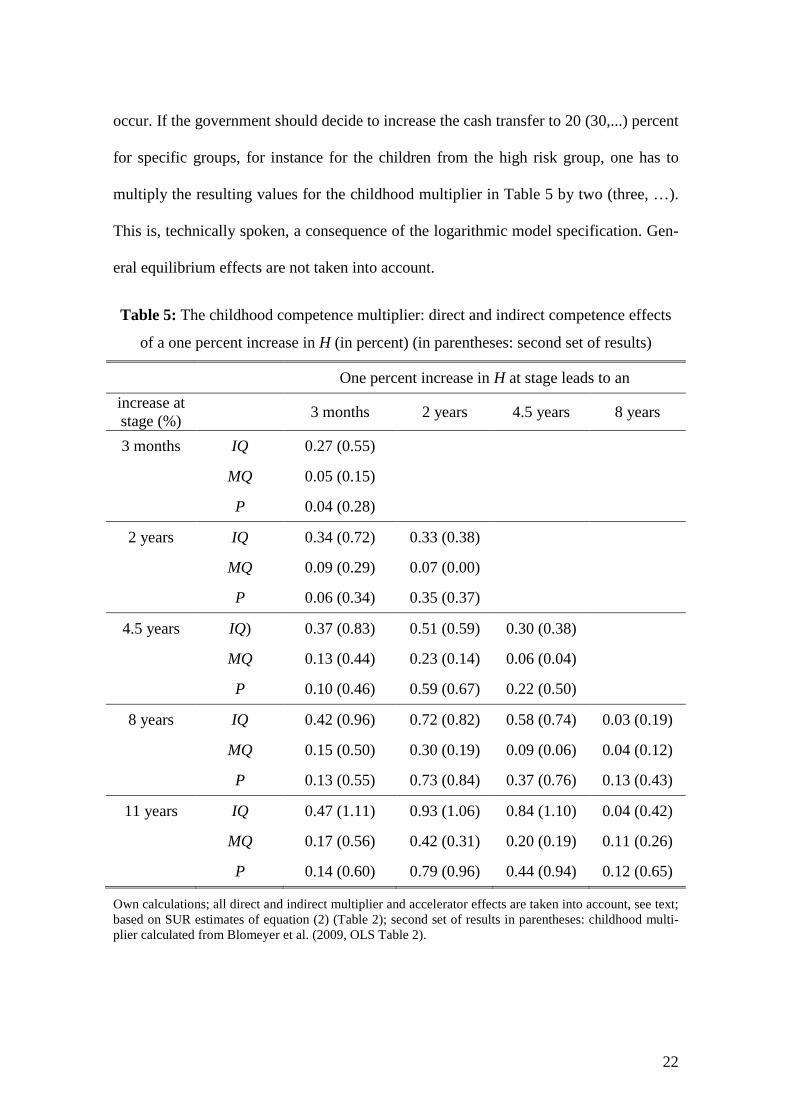
To assess the returns to higher competencies over the life cycle a sensitivity analysis
was performed, based on the idea that higher cognitive and non-cognitive competencies
increase labor market earnings (see Heineck and Anger, 2010 for a recent study with
German data). Table 6 displays the resulting discounted life cycle gains (for either 30 or
40 years) for an average worker in Germany, given that higher competencies (remember
that only policy one raises the IQ by 2.6 percent) increase annual earnings by 1, 2 or 3
percent. Results suggest that policy one would create significant returns to investments
in toddlerhood, if the income gains exceed one percent. For instance, if a 2.4 percent IQ
gain increases annual income by two percent, the expected return (for 30 years) of poli-
cy one will be 65 percent per child (((12,757.62 € - 7,725.36 €)/7,725.36€)-1)*100).
Table 6: Discounted lifetime earnings gains from a 1, 2, or 3 percent increase
in annual earnings
lifetime 1% 2% 3%
30 years 6,378.81 € 12,757.62 € 19,136.43 €
40 years 7,730.84 € 15,461.68 € 23,192.51 €
Source: Own calculations based on the average of real annual labor market earning (27.264 Euro in 1997, base year 1995; taken from Gernandt and Pfeiffer, 2007, Table A2) and a discount rate of 2 percent.
A third policy derived from the present results may aim at increasing Y and H during the
early life cycle. For instance, IQ growth until the age of eight would amount to 1.7 per-
cent (0.42+0.72+.055+0.01 percent; or 2.17 percent - 0.96+0.82+0.74+0.19 - according
to our previous findings). Such an intervention would increase the probability of enter-
ing Gymnasium by 5.7 (6.6) percent, through the boosting of competencies and re-
sources at school age. The third policy variant should be effective for improving equali-
25
ty of opportunity for children with low home resources during their early life cycle. Fu-
ture research should also investigate the costs and benefits of alternative policy inter-
ventions that take into account teaching. Improving the quality of teaching in secondary
schools may help to improve intelligence as well (see Becker et al., 2012).
8. Conclusions
This paper contributes to the understanding of competence formation and the comple-
mentarities between children’s early and later achievement in the early life cycle. Using
unique data from an epidemiological cohort study, findings demonstrate that the initial
risk matrix and the home environment are strongly related to competencies during
childhood and achievement in adolescence. Policy assessments based on the regression
results suggest that improving home resources during childhood should be an effective
way for fostering cognitive and non-cognitive competencies. Synergies in competence
formation boost social and school outcomes in adolescence as a positive side effect.
Although the evidence presented in this paper is conclusive, caveats remain and a num-
ber of research questions emerge. Since the study does not cover the population, more
research is needed with more representative data. The policy analysis utilizes the empir-
ical relationship between income per head and the socio-emotional home environment
in the data, not necessarily a causal relationship. More research should be devoted to
uncover causality between income, parental investment and the initial risk matrix. Our
measure of the home environment summarizes more than a hundred single factors that
should all be relevant for development on their own. The complex patterns of interac-
tions between these factors need further examination to understand the various facets of
the childhood multiplier for human capital formation and equality of opportunity.
26
References
Amarante, V., M. Manacorda, E. Miguel, A. Vigorito (2011), Do Cash Transfers Im-
prove Birth Outcomes? Evidence from Matched Vital Statistics, Social Security and
Program Data. NBER Working Paper No. 17690, Cambridge, MA.
Bartling, B., E. Fehr, B. Fischer, F. Kosse, M. Maréchal, F. Pfeiffer, D. Schunk, J.
Schupp, C. K. Spieß, G. G. Wagner (2010), Determinanten kindlicher Geduld – Er-
gebnisse einer Experimentalstudie im Haushaltskontext. Schmollers Jahrbuch - Jour-
nal of Applied Social Science Studies 130(3): 297-323.
Becker, M., O. Lüdtke, U. Trautwein, O. Köller, J. Baumert (2012), The Differential
Effects of School Tracking on Psychometric Intelligence: Do Academic-Track
Schools Make Students Smarter? Journal of Educational Psychology (in press).
Berger, E. M., F. H. Peter, C. K. Spieß (2011), Wie hängen familiale Veränderungen
und das mütterliche Wohlbefinden mit der frühkindlichen Bildung zusammen. DIW-
Vierteljahreshefte zur Wirtschaftsforschung 79 (3): 27-44.
Black, S. E., P. J. Devereux, K. Salvanes (2007), From the Cradle to the Labor Market?
The Effect of Birth Weight on Adult Outcomes. Quarterly Journal of Economics 122
(1): 409-439.
Blomeyer, D., K. Coneus, M. Laucht, F. Pfeiffer (2009), Initial Risk Matrix, Home Re-
sources, Ability Development and Children’s Achievement. Journal of the European
Economic Association 7(2-3): 638-648.
Blomeyer, D., M. Laucht, F. Pfeiffer, K. Reuß (2010), Mutter-Kind-Interaktion im
Säuglingsalter, Familienumgebung und Entwicklung früher kognitiver und nichtkog-
nitiver Fähigkeiten: Eine prospektive Studie. DIW-Vierteljahreshefte zur Wirt-
schaftsforschung 79 (3): 11-26.
Bradley, R. H. (1989), The Use of the HOME Inventory in Longitudinal Studies of
Child Development. P. 191-215 in: M. H. Bornstein, N. A. Krasnegar (Eds.), Stabil-
ity and continuity in mental development: Behavioral and biological perspectives.
Hillsdale, New Jersey: Lawrence Erlbaum.
Bradley, R. H., R.F.Corwyn, B.M. Caldwell, L. Whiteside-Mansell, G.A. Wassermann,
I.T. Mink (2000), Measuring the Home Environments of Children in Early Adoles-
cence. Journal of Research on Adolescence 10: 247-288.
27
Caldwell, B. M., R. H. Bradley (1984), Administration Manual (revised Edition) Home
observation for measurement of the environment. University of Arkansas at Little
Rock, Little Rock, Arkansas.
Coneus, K., M. Laucht, K. Reuß (2012), The Role of Parental Investments for cognitive
and noncognitive skill formation - Evidence for the first 11 years of life. Economics
and Human Biology 10: 189-209.
Cunha, F., J. J. Heckman (2007), The Technology of Skill Formation. The American
Economic Review 97 (2): 31-47.
Cunha, F., J. J. Heckman, S. M. Schennach (2010), Estimating the Technology of Cog-
nitive and Noncognitive Skill Formation. Econometrica 78 (3): 883-931.
Currie, J. (2011), Inequality at Birth: Some Causes and Consequences. American Eco-
nomic Review: Papers and Proceedings 101(3): 1-22.
Duckworth, A. M., M. E. P. Seligman (2005), Self-Discipline Outdoes IQ in Predicting
Academic Performance in Adolescents. American Psychological Society 16 (12):
939-944.
Gelber, A., A. Isen (2012), Children’s Schooling and Parents’ Investment in Children:
Evidence from the Head Start Study. NBER Working Paper No. w17704, Cam-
bridge, MA.
Gernandt, J., F. Pfeiffer (2007), Rising Wage Inequality in Germany. Journal of Eco-
nomics and Statistics 227 (4): 358-380.
Heckhausen, H., J. Heckhausen (2008), Motivation and Action. Cambridge, Cambridge
University Press.
Heckman, J. J. (2007), The Economics, Technology and Neuroscience of Human Capa-
bility Formation. Proceedings of the National Academy of Sciences 104 (3): 132250-
5.
Heineck, G., S. Anger (2010), The returns to cognitive abilities and personality traits in
Germany. Labour Economics 17 (3): 535-546.
Holodynski, M., F. Stallmann, D. Seeger (2008), Entwicklung als soziokultureller Lern-
prozess: Die Bildungsbedeutung von Bezugspersonen für Kinder. P. 91-129 in:
Frühkindliche Bildung und Betreuung, in T. Apolte, A. Funcke (Eds.), Nomos Ver-
lagsgesellschaft, Baden-Baden.
28
Kosse, F., F. Pfeiffer (2012), Impatience among preschool children and their mothers.
Economics Letters 115: 493-495.
Laucht, M., G. Esser, M. H. Schmidt (1997), Developmental outcome of infants born
with biological and psychosocial risks. Journal of Child Psychology and Psychiatry
38 (7): 843-854.
Laucht, M., M. H. Schmidt, G. Esser (2002), Motorische, kognitive und sozial-
emotionale Entwicklung von 11jährigen mit frühkindlichen Risikobelastungen: späte
Folgen. Zeitschrift für Kinder- und Jugendpsychiatrie und Psychotherapie 30: 5-19.
Laucht, M., M.H. Schmidt, G. Esser (2004), The development of at-risk children in ear-
ly life. Educational and Child Psychology 21 (1): 20-31.
Pfeiffer, F., K. Reuß (2008), Age-Dependent Skill Formation and Returns to Education.
Labour Economics 15 (4): 631-646.
Rutter, M., D. Quinton (1977), Psychiatric disorder – ecological factors and concepts of
causation. P. 173-187 in: Ecological factors in human development, H. McGurk
(ed.). North Holland, Amsterdam.
Spieß, C. K. (2011), Ökonomie frühkindlicher Bildung und Betreuung - Aktuelle Er-
gebnisse aus dem deutschsprachigen Forschungsraum. DIW-Vierteljahreshefte zur
Wirtschaftsforschung 79 (3): 5-10.
Statistisches Bundesamt (2011), Krankenhausstatistik, Bonn.
Todd, P. E., K. I. Wolpin (2003), On the Specification and Estimation of the Production
Function for Cognitive Achievement. The Economic Journal 113: F3-F33.
29
Table A1: Definition of organic risk
Items of the Risk Index Definition N Non-risk group: all of the items #1 to 4
1 normal birth weight 2.500–4.200 g 118
2 normal gestational age 38–42 weeks 118
3 no signs of asphyxia pHa ≥ 7.2
lactic acidb ≤ 3.5 mmol/l CTG
a score ≥ 8
118
4 no surgical delivery except elective 118
Moderate-risk group: one or more of the items #5 to #7
5 pre-eclampsia edemab proteinuriac hypertoniad
53
6 premature birth ≤ 37 weeks 151
7 signs of risk of premature birth premature labor tocolytic treatment cerclagee
43
High-risk group: one or more of the items #8 to #10
8 very low birth weight ≤ 1.500 g 46
9 clear case of asphyxia pHa ≤ 7.1
lactic acida ≥ 8.00 mmol/l CTG
b score ≤ 4
treated neonatally for ≥ 7 days
38
10 neonatal complications seizures respiratory therapy sepsis
83
aThe pH value measures an acid or basic effect of a hydrous solution. For individuals, a low pH value and lactic acid are indicators of low blood oxygen. A CTG (cardioto-cograph) measures the child’s heartbeat during pregnancy and labor, and through this, pathological values also indicate a lack of blood oxygen. bAn edema, also known as hydropsy, is the increase of interstitial fluid in any organ during swelling. cProteinuria is an indicator of possible severe damage to the metabolism or of kidney disease. dHyper-tonia is an indicator of a possible disease of the blood vessel system. eCerclage is an operative sealing of the cervix to prevent premature birth.

30
Table A2: Definition of psychosocial risk
Items of the Risk Index Definition N 1 Low educational level of a par-
ent Parent without completed school educa-tion or without skilled job training
74
2 Overcrowding More than 1.0 person per room or size of housing < 50 m2
34
3 Parental psychiatric disorder Moderate to severe axis I or II disorder according to DSM-III-Ra criteria (inter-viewer rating, kappa = .98)
76
4 History of parental broken home or delinquency
Institutional care of a parent / more than two changes of parental figures until the age of 18 or history of parental delin-quency
74
5 Marital discord Low quality of partnership in two out of three areas (harmony, communication, emotional warmth) (interviewer rating, kappa = 1.00)
43
6 Early parenthood Age of a parent < 18 years at child birth or relationship between parents lasting less than 6 months at time of conception
93
7 One-parent family At child birth 38
8 Unwanted pregnancy An abortion was seriously considered 57
9 Poor social integration and sup-port of parents
Lack of friends and lack of help in child care (interviewer rating, kappa = .71)
14
10 Severe chronic difficulties Affecting a parent lasting more than one year, such as unemployment, chronic disease (interviewer rating, kappa = .93)
104
11 Lack of coping skills Inadequate coping with stressful events of the past year e.g. denial of obvious problems, withdrawal, resignation, over-dramatization (interviewer rating, kappa = .67)
146
aThe DSM-III-R is the Diagnostic and Statistical Manual of Mental Disorders, third
edition, revised form.


![Pre Eclampsia Eclampsia[1]](https://cdn.vdocuments.site/doc/165x107/577cc41f1a28aba711982f27/pre-eclampsia-eclampsia1.jpg)


