
1
How to assess the fit of multilevellogit models with Stata?
Meeting of the German Stata User Group at theHumboldt University Berlin, June 23rd, 2017
?Models should not be true but it is important thatthey are applicable.”
John W. Tukey
Dr. Wolfgang LangerMartin-Luther-UniversitätHalle-WittenbergInstitut für Soziologie
Associate Assistant ProfessorUniversité du Luxembourg

2
Contents 1. What is the problem? 2. Summary of the econometric Monte-Carlo
studies for Pseudo R2s 3. The generalization of the McKelvey & Zavoina
Pseudo R2 for the binary and ordinal multilevellogit model
4. An application of the generalized M&Z Pseudo-and McFadden Pseudo R² in a drugconsumption study of juveniles and youngadults
5. Conclusions

3
1. What is the problem ?Current situation in applied research:
An increasing number of people uses multilevellogistic models for qualitative dependent variableswith binary and ordinal outcome
But users often complain that there are no fitmeasures for these models
Neither Stata 14 / 15 nor SPSS 24 offer any fitmeasure for these models
Let me demonstrate how to generalize the PseudoR2s for binary and ordinal logit model for themultilevel analysis

4
Which solutions does Stata provide?
Indeed Stata estimates multilevel logit models forbinary, ordinal and multinomial outcomes (melogit,meologit, gllamm) but it does not calculate anyPseudo R2. It provides only the information criteriaAIC and BIC (estat ic)
Stata provides a Wald-test for the fixed-effectsand a Likelihood-Ratio-χ2 test for the randomeffects of the exogenous variables
Even special purpose programs like HLM, MlwiN,MPLUS or SuperMix do not calculate any PseudoR2

5
Raudenbush & Bryk (2002), Heck & Thomas(2009) and Rabe-Hesketh & Skrondal (2013) donot mention Peudo R2s
Snijder & Bosker(2012) propose a variation ofMcKelvey & Zavoina Pseudo R2 for random-intercept- and intercept-as-outcome logit models.It is not implemented in any program
Hox (2010) discusses the McFadden, Cox & Snell,Nagelkerke and McKelvey & Zavoina Pseudo R2. He recommends the last one to assess the modelfit
What can we learn from multilevelliterature?

6
2. Summary of the econometric Monte-Carlo studies for testing Pseudo R2s
Econometricians made a lot of Monte-Carlostudies in the early 90s:
< Hagle & Mitchell 1992< Veall & Zimmermann 1992, 1993, 1994< Windmeijer 1995< DeMaris 2002
They tested systematically the mostcommon Pseudo-R²s for binary and ordinalprobit / logit models
7
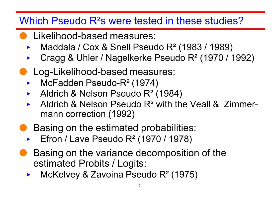
Which Pseudo R²s were tested in these studies? Likelihood-based measures:< Maddala / Cox & Snell Pseudo R² (1983 / 1989)< Cragg & Uhler / Nagelkerke Pseudo R² (1970 / 1992)
Log-Likelihood-based measures:< McFadden Pseudo-R² (1974)< Aldrich & Nelson Pseudo R² (1984)< Aldrich & Nelson Pseudo R² with the Veall & Zimmer-
mann correction (1992) Basing on the estimated probabilities:< Efron / Lave Pseudo R² (1970 / 1978)
Basing on the variance decomposition of theestimated Probits / Logits:
< McKelvey & Zavoina Pseudo R² (1975)

8
Results of the Monte-Carlo-Studies forbinary and ordinal logits or probits The McKelvey & Zavoina Pseudo R² is the best
estimator for the ?true R²” of the OLS regression The Aldrich & Nelson Pseudo R² with the Veall &
Zimmermann correction is the best approximation ofthe McKelvey & Zavoina Pseudo R²
Lave / Efron, Aldrich & Nelson, McFadden and Cragg& Uhler Pseudo R² severely underestimate the ?trueR²” of the OLS regression
My personal advice: < Use the McKelvey & Zavoina Pseudo R² to assess the fit
of binary and ordinal logit models
9
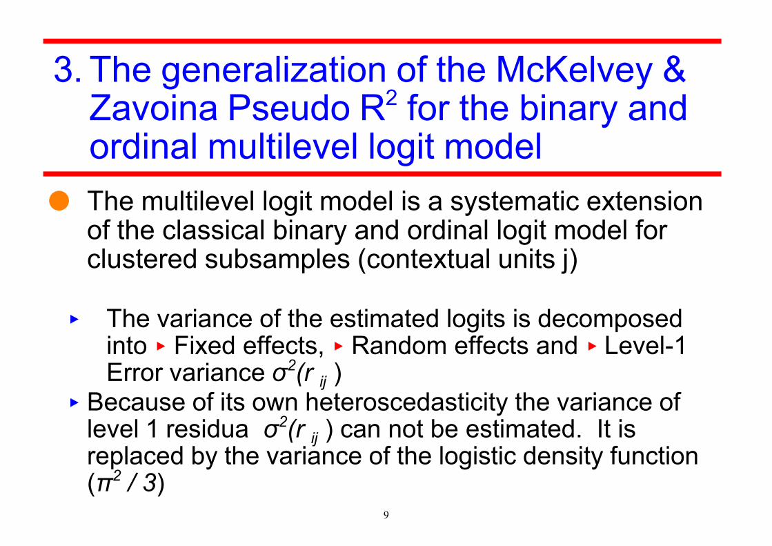
3. The generalization of the McKelvey & Zavoina Pseudo R2 for the binary andordinal multilevel logit model
The multilevel logit model is a systematic extensionof the classical binary and ordinal logit model for clustered subsamples (contextual units j)
< The variance of the estimated logits is decomposedinto < Fixed effects, < Random effects and < Level-1Error variance σ2(r ij )
< Because of its own heteroscedasticity the variance oflevel 1 residua σ2(r ij ) can not be estimated. It isreplaced by the variance of the logistic density function (π2 / 3)

2
2* *
1*2
* 2* *
13
ˆ ˆˆ
&ˆ ˆ ˆ
n
ii
n
ii
y yVar y nM Z Pseudo R
Var y Var y y
n
:*yi
:*y 2
3 :
Var y :*
10
McKelvey & Zavoina Pseudo R2 (M & Z Pseudo R2)
Let’s have a short look at the lucky winner
Range: 0 # M & Z-Pseudo R² #1Legend:
Expected value of the estimated logits
Estimated logit of case i
Variance of the logistic density function
Variance of the estimated logits (latent variable Y*)

11
Generalization to the 2-level logit model 2 Prediction of the latent variable Y* (estimated binary
or cumulative logit) in two ways< Population-Average Prediction with the fixed effects of
the exogenous variables (all random effects hold at zero)– Stata-command: predict newvar1 if e(sample), xb
< Unit-Specific Prediction of the fixed and random effectsof the exogenous variable– Stata-command: predict newvar2 if e(sample), eta
Therefore, the variance of the estimated logits (Y*)can be calculated in two different ways
< Only for the fixedeffects of the exogenous variables< For the fixed and random effects of the exogenous
variables

12
Generalization to the 2-level logit model 3
Therefore we get two different McKelvey &Zavoina Pseudo R2s
< ?Population-Average” M & Z Pseudo R2 (fixed effects)< ?Unit-Specific” M & Z PseudoR2 (fixed- & random
effects)
For the ?Unit-Specific” M & Z Pseudo R2 usesestimated fixed and random effects for prediction,it assesses the fit more realistically as its?Population-Average” counterpart
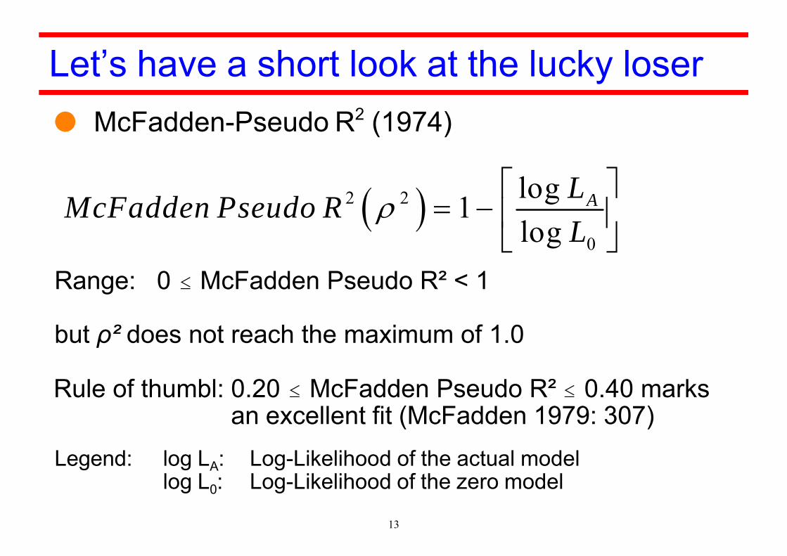
2 2
0
log1log
ALMcFadden Pseudo RL
13
McFadden-Pseudo R2 (1974)
Let’s have a short look at the lucky loser
Range: 0 # McFadden Pseudo R² < 1
but ρ² does not reach the maximum of 1.0
Legend: log LA: Log-Likelihood of the actual model log L0: Log-Likelihood of the zero model
Rule of thumbl: 0.20 # McFadden Pseudo R² # 0.40 marksan excellent fit (McFadden 1979: 307)
14
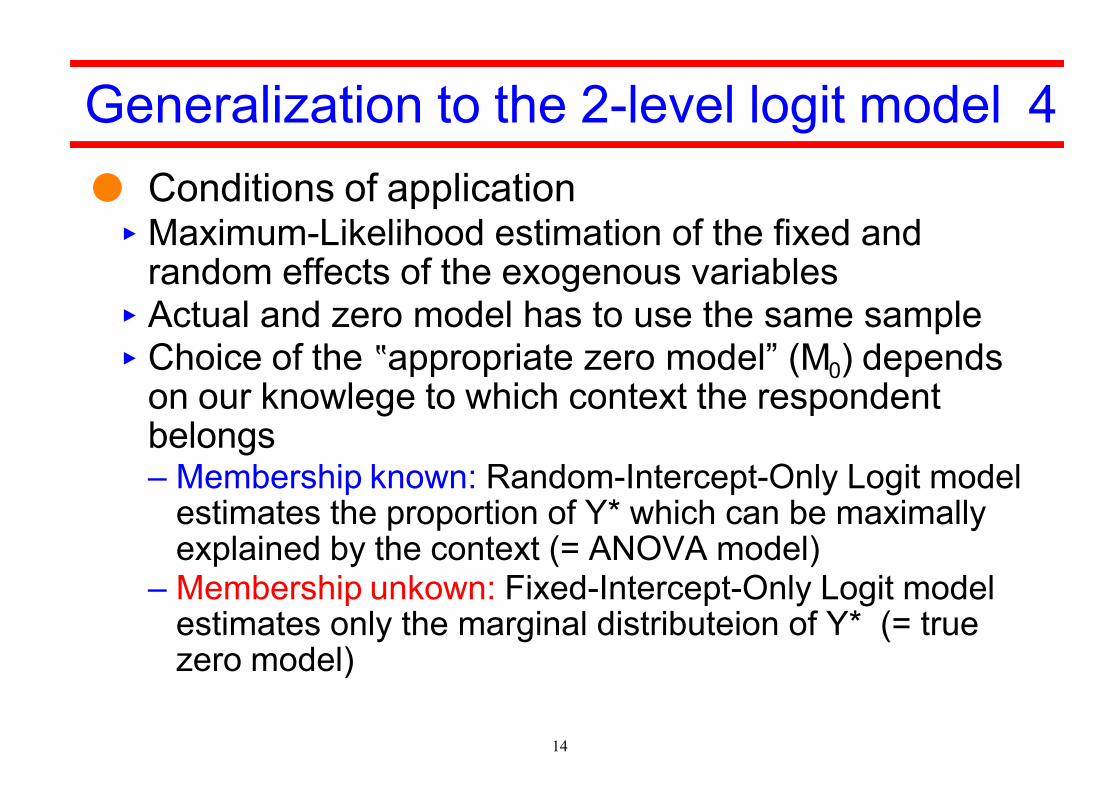
Generalization to the 2-level logit model 4 Conditions of application< Maximum-Likelihood estimation of the fixed and
random effects of the exogenous variables< Actual and zero model has to use the same sample < Choice of the ?appropriate zero model” (M0) depends
on our knowlege to which context the respondentbelongs– Membership known: Random-Intercept-Only Logit model
estimates the proportion of Y* which can be maximallyexplained by the context (= ANOVA model)
– Membership unkown: Fixed-Intercept-Only Logit modelestimates only the marginal distributeion of Y* (= truezero model)

15
Generalization to the 2-level logit model 5 Calculation of McFadden Pseudo R2 is possible in two
different ways using the following as a zero model< Random-Intercept-Only Logit-Model
– It measures the proportional reduction of the log likelihood ofthe actual model caused by the fixed effects of the exogen-ous variables in comparison to the RIOM
– Its Likelihood-Ratio χ2 test refers to all fixed effects of theexogenous level 1 and level 2 variables
< Fixed-Intercept-Only Logit-Model– It measures the proportional reduction of the log likelihood of
the actual model caused by fixed and random effects of allexogenous variables in comparison to the FIOM
– Its Likelihood-Ratio χ2 test refers to all fixed and randomeffects of the exogenous level 1 and level 2 variables

16
4. Example of application Flash Eurobarometer No 330 about youth
attitudes on drugs (2011)< WebCATI-Survey of nij = 12.313 respondents (aged
15 - 24) in n.j = 27 EU member states (contextualunits j)
< My focus: – prevalence of cannabis use by juveniles and young
adults (q10): Have you used cannabis by yourself?– 1) never – 2) more than 12 months ago– 3) less than 12 months ago– 4) in the last 30 days
< Let us have a look at the exogenous variables in thefollowing diagram
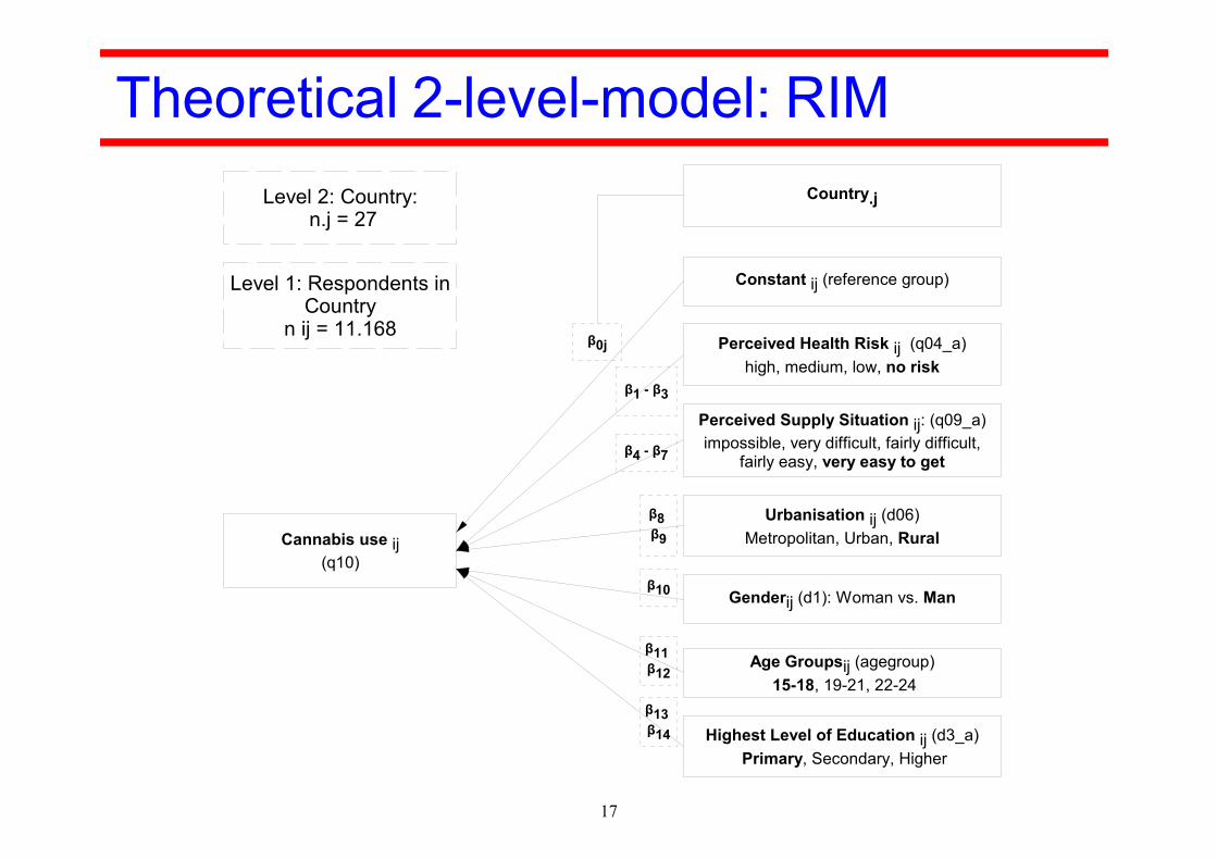
Cannabis use ij(q10)
Perceived Health Risk ij (q04_a)high, medium, low, no risk
Perceived Supply Situation ij: (q09_a)impossible, very difficult, fairly difficult,
fairly easy, very easy to get
Genderij (d1): Woman vs. Man
Age Groupsij (agegroup)15-18, 19-21, 22-24
Highest Level of Education ij (d3_a) Primary, Secondary, Higher
Urbanisation ij (d06)Metropolitan, Urban, Rural
Constant ij (reference group)
Country.j
β1 - β3
β4 - β7
β8 β9
β10
β11 β12
β0j
Level 2: Country: n.j = 27
Level 1: Respondents in Country
n ij = 11.168
β13 β14
17
Theoretical 2-level-model: RIM

18
Stata-OutputVersion14
LR test vs. ologit model: chibar2(01) = 222.09 Prob >= chibar2 = 0.0000------------------------------------------------------------------------------------------- var(_cons)| .2623196 .0849424 .1390597 .494835country |--------------------------+---------------------------------------------------------------- /cut3 | 1.857033 .1357061 13.68 0.000 1.591053 2.123012 /cut2 | .6715688 .133064 5.05 0.000 .4107681 .9323695 /cut1 | -.4269461 .1329725 -3.21 0.001 -.6875674 -.1663248--------------------------+---------------------------------------------------------------- higher education | -.0415283 .099673 -0.42 0.677 -.2368837 .1538271 secondary education | -.0345302 .0753855 -0.46 0.647 -.1822832 .1132227 d3_a | | 22 - 24 | .6847313 .0797637 8.58 0.000 .5283974 .8410652 19 - 21 | .4924681 .073827 6.67 0.000 .3477699 .6371663 agegroup | | female | -.4654088 .0504709 -9.22 0.000 -.5643298 -.3664877 d1 | | other town/urban centre | .196061 .0606935 3.23 0.001 .0771039 .315018 metropolitan zone | .3536598 .0713306 4.96 0.000 .2138545 .4934652 d6 | | fairly easy | -.6291072 .0553719 -11.36 0.000 -.7376341 -.5205803 fairly difficult | -1.555672 .0870857 -17.86 0.000 -1.726357 -1.384987 very difficult | -2.191986 .1207629 -18.15 0.000 -2.428677 -1.955295 impossible | -3.006983 .1899514 -15.83 0.000 -3.379281 -2.634685 q9_a | | low risk | -.7425748 .0611709 -12.14 0.000 -.8624676 -.622682 medium risk | -1.696693 .0730464 -23.23 0.000 -1.839861 -1.553525 high risk | -2.670499 .1092326 -24.45 0.000 -2.884591 -2.456407 q4_a |--------------------------+---------------------------------------------------------------- q10ord | Coef. Std. Err. z P>|z| [95% Conf. Interval]-------------------------------------------------------------------------------------------Log likelihood = -7410.7117 Prob > chi2 = 0.0000 Wald chi2(14) = 2142.78
Integration method: mvaghermite Integration pts. = 7
max = 490 avg = 413.6 min = 211 Obs per group:
Group variable: country Number of groups = 27Mixed-effects ologit regression Number of obs = 11,168
Fixed effects
Thresholds Random effect

19
What does Stata offer to assess the fit? Akaike (AIC) und Schwarz Bayesian Information
Criterion (BIC)< Decision rule:Choose the model with the lowest AIC or
BIC
< Looking at AIC and BIC, the rim fits best of all badmodels
< But we do not know how well the rim fits
Note: N=Obs used in calculating BIC; see [R] BIC note.----------------------------------------------------------------------------- rim | 11,168 . -7410.712 18 14857.42 14989.2 riom | 11,168 . -9033.234 4 18074.47 18103.75 fiom | 11,168 . -9326.802 3 18659.6 18681.57-------------+--------------------------------------------------------------- Model | Obs ll(null) ll(model) df AIC BIC-----------------------------------------------------------------------------
Akaike's information criterion and Bayesian information criterion
. estimates stats fiom riom rim

20
Assessing the fit by the McKelvey & Zavoina-PseudoR2s and the Intra-Class-Correlation
Output of my fit_melogit_2lev.ado 1
Intra-Class-Correlation (Level 2) = 0.1507 Just estimating the Random-/Fixed Intercept Only Logit-Model McKelvey&Zavoina-Pseudo-R2 (fixed effects only)= 0.4774 McKelvey&Zavoina-Pseudo-R2 (fixed&random effects)= 0.5137 Fit-measures for the MELOGIT/MEOLOGIT-model:. fit_meologit_2lev
21
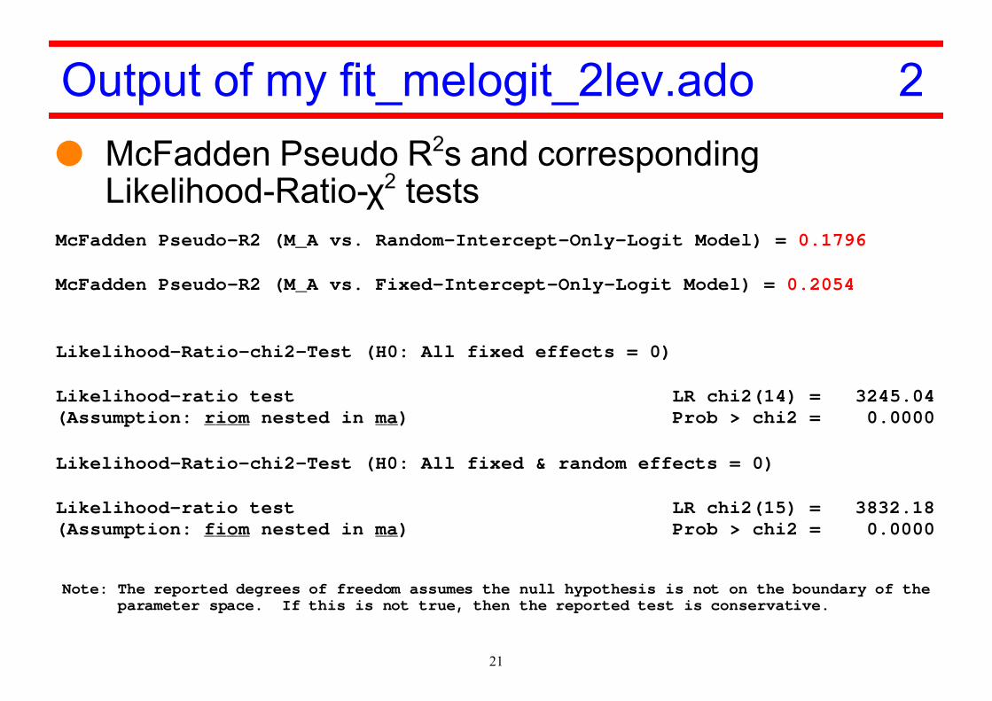
McFadden Pseudo R2s and correspondingLikelihood-Ratio-χ2 tests
Output of my fit_melogit_2lev.ado 2
parameter space. If this is not true, then the reported test is conservative.Note: The reported degrees of freedom assumes the null hypothesis is not on the boundary of the
(Assumption: fiom nested in ma) Prob > chi2 = 0.0000Likelihood-ratio test LR chi2(15) = 3832.18
Likelihood-Ratio-chi2-Test (H0: All fixed & random effects = 0) (Assumption: riom nested in ma) Prob > chi2 = 0.0000Likelihood-ratio test LR chi2(14) = 3245.04
Likelihood-Ratio-chi2-Test (H0: All fixed effects = 0) McFadden Pseudo-R2 (M_A vs. Fixed-Intercept-Only-Logit Model) = 0.2054 McFadden Pseudo-R2 (M_A vs. Random-Intercept-Only-Logit Model) = 0.1796

22
The baseline
How does the effects look like?
39.49%
26.7%
20.31%
13.51%
never more than 12 monthsless than 12 months last 30 days
Estimated probabilities of cannabis use for the reference group

23
The joint marginsplot for the 4 categories
Effects with Respect to
never more than 12 monthsless than 12 months last 30 days
Conditional Marginal Effects with 95% CIs

24
5. Conclusions 1
Known< The Monte-Carlo-simulation studies show that the
McKelvey & Zavoina Pseudo R² is the best fit measurefor binary and ordinal logit models
New< Generalization of the M & Z-Pseudo R2 to binary and
ordinal multilevel logit models. The prediction ofestimated logits bases upon the fixed effects only orupon fixed and random effects of exogenous variables
< The McFadden-Pseudo R2 bases upon the fixed effectsonly or upon fixed and random-effects of the exogenousvariables using a context-independent zero model

25
5. Conclusions 2
New< Simultaneous Likelihood-Ratio-χ2 test for the
estimated fixed effects using the random-intercept-only (RIOM) as the zero model
< Simultaneous Likelihood-Ratio-χ2 test for theestimated fixed and random effects using the fixed-intercept-only (FIOM) as the zero model
That’s why< I suggest to use my fit_meologit_2lev.ado and
fit_meologit_3lev.ado to assess the fit of 2- and 3-level logit models with binary and ordinal outcome

26
Closing words
Thank you for your attention
Do you have some questions?

27
Contact
Affiliation
< Dr.Wolfgang LangerUniversity of HalleInstitute of SociologyD 06099 Halle (Saale)
< Email: [email protected]

28
Stata code for fit_meologit_2lev.ado 1program fit_meologit_2lev, rclassversion 14
tempvar plgt1
quietly estimates store ma
quietly predict `plgt1' if e(sample), eta
quietly sum `plgt1'
display as text "Fit-measures for the MELOGIT/MEOLOGIT-model:"display as text " " display as text "McKelvey&Zavoina-Pseudo-R2 (fixed&random effects)= " as result %6.4f /// abs(r(Var)*r(N)-1) / ((r(N)*(_pi^2 / 3)+ (r(Var)*r(N)-1))) display as text " " drop ̀ plgt1'
tempvar plgt2quietly predict `plgt2' if e(sample), xb
quietly sum `plgt2'
display as text "McKelvey&Zavoina-Pseudo-R2 (fixed effects only)= " as result %6.4f /// abs(r(Var)*r(N)-1) / ((r(N)*(_pi^2 / 3)+ (r(Var)*r(N)-1)))
drop ̀ plgt2'
dis " "
capture drop llma
tempvar llma
gen llma=`e(ll)'
dis as text " "dis as text "Just estimating the Random-/Fixed Intercept Only Logit-Model"dis as text " "

29
Stata code for fit_meologit_2lev.ado 2* Schaetzung des RIOMquietly: `e(cmd2)' `e(depvar)' if e(sample), || `e(ivars)':
quietly: estimates store riom
* Berechnung der Intra-Class-Correlation (ICC)display as text "Intra-Class-Correlation (Level 2) = " as result %6.4f /// (_b[var(_cons[`e(ivars)']):_cons]) / (_b[var(_cons[`e(ivars)']):_cons] + (_pi^2 / 3))
dis as text " "dis as text "McFadden Pseudo-R2 (M_A vs. Random-Intercept-Only-Logit Model) = " /// as result %6.4f abs(1- (llma /`e(ll)'))dis as text " "
* Schätzung des FIOMquietly: `e(cmd2)' `e(depvar)' if e(sample)
quietly: estimates store fiom
dis as text "McFadden Pseudo-R2 (M_A vs. Fixed-Intercept-Only-Logit Model) = " /// as result %6.4f abs(1- (llma /`e(ll)'))dis as text " "
drop llma
dis as text " " dis as text "Likelihood-Ratio-chi2-Test (H0: All fixed effects = 0) "lrtest riom ma
dis as text " " dis as text "Likelihood-Ratio-chi2-Test (H0: All fixed & random effects = 0) "lrtest fiom ma
exit

30
Appendix

0j 01 . 0
1j 10 11 . 1
0 1j
Level2: Between-Context Regression2a)LogisticIntercept-as-Outcome-Model:
0
2b)LogisticSlope-as-Outcome-Model:
Level1: Within-Context Regression
P Y > 1) ln
P Y
j j
j j
j
Z u
Z u
kk
1
1
1
01 . 0 10 11 . 11
{ }
Single equation notation: 2a) and 2b) in 1)
P Y > ln 0 { }
P Y
k
ij k ijK
K
j j ij ij j j ij k ijk
X r
kZ u X X Z u X r
k
31
Multilevel ordered logit model 1 Equations of the 2-level-ordered logit model
Notation of Raudenbush&Bryk(2002):
γ: fixed-effect estimatorZ: exogenous level 2 variableβ: random-effect estimatorX: exogenous level 1 variableu0j: residuum random-interceptu1j: residuum random-sloperij: residuum of within-context-
logistic regressionδk: threshold for kategory k of Y
0 0 00 01 . 0 0
1 1 10 11 . 1 1
3 )
3 )
j j j j j
j j j j j
a u Z
b u Z
2
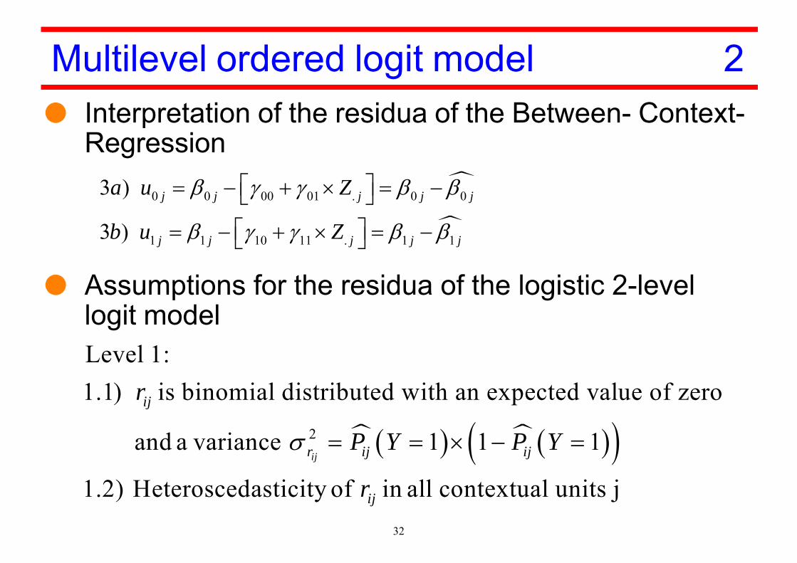
Level 1:1.1) is binomial distributed with an expected value of zero
and a variance 1 1 1
1.2) Heteroscedasticity of in all contextual units jij
ij
r ij ij
ij
r
P Y P Y
r
32
Multilevel ordered logit model 2 Interpretation of the residua of the Between- Context-
Regression
Assumptions for the residua of the logistic 2-level logit model

0 1
0 1
k j
0 0 0 0 1 2 20 0 1 1
1 1 0 1 1
, 1 0 0 1
2 .1) u is n o rm al d is trib u ted w ith an ex p ec ted va lu e o f ze ro an d
a co varian ce m atrix T o f th e res id u a
00
2 .2 ) T h e res id u a o f leve l1 an d
j j
j j
ju u
j
u u
uE
u
0 1, ,
leve l 2 are n o t co rre la ted :0
j ij j iju r u r
33
Multilevel ordered logit model 3
Residua of level 2
Implication for the level 1 residuum rij< Because of its own heteroscedasticity the variance σ2(rij)
can not be estimated. It is replaced by the variance of thelogistic density function (π2 / 3)

2 log 2
2 log log
Range: 00
complexitdevianc yof themode
:log
e
:::
l
A
A
M
M
AIC L k
BIC L N k
AICBIC
LegendLogarithmusnaturalis
k Numberof estimated parametersN Samplesize
34
Calculation of Akaike- (AIC) and Schwarz Bayesian-Information-Criteria (BIC)
Alternative in Stata: Information criteria

35
References– Aldrich, J.H. & Nelson, F.D. (1984):
Linear probability, logit, and probit models. Newbury Park: SAGE(Quantitative Applications in the Social Sciences, 45)
– Amemiya, T. (1981):Qualitative response models: a survey. Journal of Economic Literature, 21,pp.1483-1536
– Begg, C.B. & Gray, R. (1984):Calculation of polychotomous logistic regression parameters using individualizedregression. Biometrika, 71, pp.11-18
– Ben-Akiva,M. & S.R.Lerman 19914(1985): Discrete choice analysis. Theory andapplication to travel demand. Cambridge, Mass: MIT-Press
– Cox, D.R.& Snell, E.J. (1989): The analysis of binary data. London: Chapman&Hill– Cragg, S.G.& Uhler, R. (1970):
The demand for automobiles. Canadian Journal of Economics, 3, pp. 386-406– DeMaris, A.(2002):
Explained variances in logistic regression. A Monte Carlo study of proposedmeasures. Sociological Methods&Research, 11, 1, pp. 27-74
– Efron, B. (1978):Regression and Anova with zero-one data. Measures of residual variation. Journalof American Statistical Association, 73, pp. 113-121
– Hagle, T.M. & Mitchell II,G.E. (1992):Goodness of fit measures for probit and Logit. American Journal of PoliticalScience, 36, 3, pp. 762-784
– Heck, R.H.&Thomas S.L. (2009): An Introduction to Multilevel Modeling Techniques. New York, N.Y.: Routlege
– Hensher, D.A.& Johnson, L.W. (1981):Applied discrete choice modelling. London: Croom Helm

36
References 2
– Hensher, D.A., Rose, J.M. & Greene (2005): Applied choice analysis. A primer. Cambridge: Cambridge University Press
– Hox, J.J. (2010²): Multilevel Analysis. Techniques and Applications. New York, NY: Routledge– Huq, N.M.& Cleland, J. (1990): Bangladesh Fertility Surey 1989 (Main Report). Dhaka: National
Institute of Population Research and Training – Long, J.S. (1997):
Regression models for categorical and limited dependent variables. Thousand Oaks, Ca : Sage– Long, J.S. & Freese, J. (2000):
Scalar measures of fit for regression models. Bloomington, : Indiana University– Long, J.S. & Freese, J. (20032):
Regression models for categorical dependent variables using Stata. College Station, Tx: Stata– Maddala, G.S. (1983):
Limited-dependent and qualitative variables in econometrics. Cambridge: Cambridge University Press
– McFadden, D. (1979):Quantitative methods for analysing travel behaviour of individuals: some recent developments.
In: Hensher, D.A.& Stopher, P.R.: (eds):Behavioural travel modelling. London: CroomHelm, pp. 279-318
– McKelvey, R. & Zavoina, W. (1975):A statistical model for the analysis of ordinal level dependent variables. Journal of Mathematical
Sociology, 4, pp. 103-20– Nagelkerke, N.J.D. (1991):
A note on a general definition of the coefficient of determination. Biometrika, 78, 3, pp.691-693

37
References 3
– Ronning, G. (1991): Mikro-Ökonometrie. Berlin: Springer– Rabe-Hesketh, S. & Skrondal, A.(2012³): Multilevel and Longitudinal Modeling Using Stata. Volume II:
Categorical Responses, Counts, and Survival. Collage Station, Tx: Stata Press– Raudenbush, S.W. & Bryk, A.S. (2002²): Hierarchical Linear Models. Applications and Data Analysis
Methods. Thousand Oaks, CA: Sage– Snijders, T.A.B.&Bosker, R.J.(2012²): Multilevel Analysis. An Introduction to Basic and Advanced
Multilevel Modeling. Thousand Oaks, CA: Sage– Veall, M.R. & Zimmermann, K.F. (1992):
Pseudo-R2 in the ordinal probit model. Journal of Mathematical Sociology, 16, 4, pp. 333-342– Veall, M.R. & Zimmermann, K.F. (1994):
Evaluating Pseudo-R2's for binary probit models. Quality&Quantity, 28, pp. 151- 164– Windmeijer, F.A.G. (1995):
Goodness-of-fit measures in binary choice models. Econometric Reviews, 14, 1, pp. 101-116– Zimmermann, K.F. (1993):
Goodness of fit in qualitative choice models: review and evaluation. In: Schneeweiß, H. &Zimmermann, K. (eds): Studies in applied econometrics. Heidelberg: Physika, pp. 25-74


