Higher Spins & Strings
Matthias Gaberdiel
ETH Zürich
The Mathematics of CFT
ANU Canberra
13 July 2015
Based mainly on work with Rajesh Gopakumar,
1011.2986, 1106.1897, 1205.2472, 1305.4181,1406.6103, 1501.07236

AdS / CFT duality
Much recent progress in string theory has been related to AdS/CFT duality
AdS5 × S5
superstrings on SU(N) super Yang-Mills theory in 4 dimensions
=
4d non-abelian gauge theory similar to that appearing in the standard model of particle physics.
[Maldacena, ‘97, ...]

(
R
lPl
⇥4
= N
Relation of parameters
(
R
ls
⇥4
= g2
YMN = λgstring = g
2YM
The relation between the parameters of the two theories is
AdS radius in string units
‘t Hooft parameter
AdS radius in Planck units

Strong weak duality
For example, in the large N limit of gauge theory at large ‘t Hooft coupling
Supergravity (point particle) approximation is good for AdS description.
largelarge
(
R
lPl
⇥4
= N
(
R
ls
⇥4
= g2
YMN = λgstring = g
2YM
small
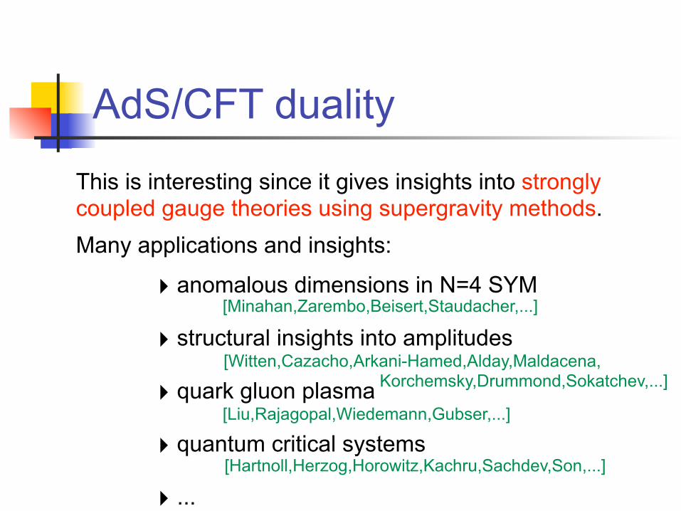
AdS/CFT duality
This is interesting since it gives insights into strongly coupled gauge theories using supergravity methods.
Many applications and insights:
‣ anomalous dimensions in N=4 SYM
‣ structural insights into amplitudes
‣ quark gluon plasma
‣ quantum critical systems
‣ ...
[Hartnoll,Herzog,Horowitz,Kachru,Sachdev,Son,...]
[Liu,Rajagopal,Wiedemann,Gubser,...]
[Witten,Cazacho,Arkani-Hamed,Alday,Maldacena, Korchemsky,Drummond,Sokatchev,...]
[Minahan,Zarembo,Beisert,Staudacher,...]

Conceptual understanding
However, at present, we are far from a conceptual understanding of why the duality works, and what ingredients are crucial for it, e.g. whether it requires
supersymmetry integrability ...
This is obviously an important question since in many applications these features are absent.

ls →∞
Weakly coupled gauge theory
In order to make progress in this direction analyse another corner of AdS/CFT: consider case where gauge theory is weakly coupled
small
`tensionless strings’[Sundborg, ‘01] [Witten, ‘01] [Sezgin,Sundell, ‘01]
(
R
lPl
⇥4
= N
(
R
ls
⇥4
= g2
YMN = λgstring = g
2YM
large

Higher spin theory
Resulting theory has an infinite number of massless higher spin fields, which generate a very large gauge symmetry.
maximally unbroken phase of string theory
effective description in terms of Vasiliev Higher Spin Theory.

Leading Regge trajectory
On the dual CFT side, the traces of bilinears of elementary Yang-Mills fields form closed subsector in free theory.
This subsector is believed to correspond to the leading Regge trajectory from the string point of view:
`vector-like’ HS -- CFT duality

[Chang, Minwalla, Sharma, Yin, ‘12] [MRG, Gopakumar, ‘14]
State of the Art
In the past this idea was taken as a general motivation to consider dualities relating
Vasiliev HS theory
on AdS
vector-like weakly coupled
CFT
However, recently interesting progress about how these dualities fit actually into stringy AdS/CFT correspondence has been made....

WN,k
λ =N
N + kand M
2 = −(1− λ2)
3d proposal
Concrete duality of this kind (somewhat similar to Klebanov & Polyakov proposal for AdS4/CFT3)
λ
AdS3: higher spin theory with a complex scalar of mass M
2d CFT: minimal models in large N ‘t Hooft limit with coupling
where
[MRG,Gopakumar, ‘10]

Outline
This version of the duality is bosonic, but can nevertheless be tested in quite some detail. In particular, we can match
‣ quantum symmetries
‣ spectrum
At the end I will also explain how this higher spin duality relates to stringy AdS3 -- CFT2 duality.

hs[λ] ⊕ C ⇠=U(sl(2))
hC2 −1
4(λ2 − 1)1i
sl(2,R) → hs[λ] ∼= sl(λ)
The HS theory on AdS3
Recall that pure gravity in AdS3: Chern-Simons theory based on [Achucarro, Townsend, ‘86]
[Witten, ‘88]
Higher spin description: replace [Prokushkin, Vasiliev, ‘98]
The AdS3 HS theory can be described very simply.
where [Bergshoeff et.al. ‘90]
[Pope, Romans, Shen, ‘90]
[Fradkin, Linetsky, ‘91]
[one spin field for each spin ]
sl(2, R)
s = 2, 3, . . .

V s
nwith |n| < s , s = 2, 3, . . .
hs[λ] :
Higher spin algebra
Generators of
`wedge algebra’
W∞[λ] algebra
For these higher spin theories asymptotic symmetry algebra can be determined following Brown & Henneaux, leading to classical
[Henneaux & Rey, ‘10] [Campoleoni et. al. ‘10] [MRG, Hartman, ‘11]

L0, L±1 → Ln , n ∈ Z
sl(2, R)
hs[λ] → W∞[λ]
s = 2, . . . ,∞, n ∈ Z
Asymptotic symmetry algebra
Asymptotic symmetry algebra extends hs algebra `beyond the wedge’:
pure gravity:
higher spin:
[Figueroa-O’Farrill et.al. ‘92]
(Virasoro)
generated by Vs
n

W∞[λ] = limN→∞
WN,k with λ =N
N + k.
Dual CFT
By the usual arguments, dual CFT should therefore have
Basic idea:
‘t Hooft limit of 2d CFT!
W∞[λ] symmetry.

WN,k :su(N)k ⊕ su(N)1
su(N)k+1
The minimal models
The minimal model CFTs are the cosets
General N: higher spin analogue of Virasoro minimal models. [Spin fields of spin s=2,3,..,N.]
e.g. Ising model (N=2, k=1) tricritical Ising (N=2, k=2) 3-state Potts (N=3,k=1),..
cN (k) = (N − 1)[
1−N(N + 1)
(N + k)(N + k + 1)
⇥
.
with central charge
[Bais et.al., ‘88] [Bouwknegt, Schoutens, ‘92]

W∞[λ]
Relation of symmetries
is a classical (commutative) Poisson algebra.
In order to understand relation to minimal model W-algebras, need to understand how to quantise it.
The asymptotic symmetry algebra
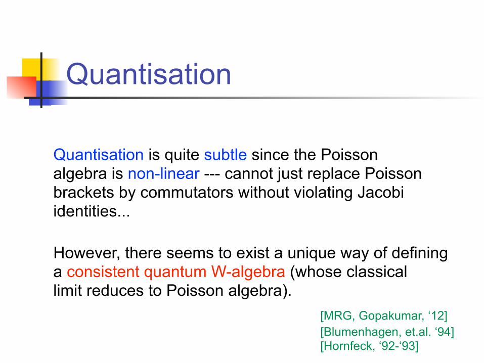
Quantisation
Quantisation is quite subtle since the Poisson algebra is non-linear --- cannot just replace Poisson brackets by commutators without violating Jacobi identities...
However, there seems to exist a unique way of defining a consistent quantum W-algebra (whose classical limit reduces to Poisson algebra).
[MRG, Gopakumar, ‘12]
[Blumenhagen, et.al. ‘94] [Hornfeck, ‘92-‘93]

[W 3m
, W 3n] = 2(m− n)W 4
m+n+
N3
12(m− n)(2m2 + 2n2
−mn− 8)Lm+n
+8N3
c(m− n) (LL)m+n +
N3c
144m(m2
− 1)(m2− 4)δm,−n
Quantum symmetry
[MRG, Gopakumar, ‘12]
There are two steps to this argument. To illustrate them consider an example. Naive quantisation of classical algebra leads to
spin-3 field
non-linear term

Jacobi identity
spin-3 field
non-linear term
[W 3m
, W 3n] = 2(m− n)W 4
m+n+
N3
12(m− n)(2m2 + 2n2
−mn− 8)Lm+n
+8N3
c(m− n) (LL)m+n +
N3c
144m(m2
− 1)(m2− 4)δm,−n

Λ(4)n
=X
p
: Ln−pLp : +15xnLn
[W 3m
, W 3n] = 2(m− n)W 4
m+n+
N3
12(m− n)(2m2 + 2n2
−mn− 8)Lm+n
+8N3
c + 225
(m− n) Λ(4)m+n
+N3c
144m(m2
− 1)(m2− 4)δm,−n
Jacobi identity
Jacobi identity determines quantum correction
where
Similar considerations apply for the other commutators.
[W 3m
, W 3n] = 2(m− n)W 4
m+n+
N3
12(m− n)(2m2 + 2n2
−mn− 8)Lm+n
+8N3
c(m− n) (LL)m+n +
N3c
144m(m2
− 1)(m2− 4)δm,−n

W(3)
· W(3)
∼
c
3· 1 + 2 · L +
32
(5c + 22)· Λ(4) + 4 · W
(4)
W(3)
· W(4)
∼ C433 · W
(3)+ · · ·
(
C4
33
)2=
64
5
λ2 − 9
λ2 − 4+ O( 1
c) .
Structure constants
The second step concerns structure constants. The fields can be rescaled so that
but then coupling constant
characterises algebra. Classical analysis determines
[MRG, Hartman, ‘11]

Structure constants
Classical analysis determines
(
C4
33
)2=
64
5
λ2 − 9
λ2 − 4+ O( 1
c) .

λ = N WN :
Structure constants
Classical analysis determines
Requirement that representation theory agrees for with
hs[λ]∣
∣
∣
λ=N
∼= sl(N, R)[Note: implies .] W∞[λ]|λ=N
= WN
(
C4
33
)2=
64
5
λ2 − 9
λ2 − 4+ O( 1
c) .
γ2≡
(
C4
33
)2=
64 (c+ 2) (λ− 3)(
c(λ+ 3) + 2(4λ+ 3)(λ− 1))
(5c+ 22) (λ− 2)(
c(λ+ 2) + (3λ+ 2)(λ− 1)) .

λ = 0 :
λ = 1 :
Explicit check
This formula has also been checked explicitly for the two special cases:
N complex bosons giving c=2N
N complex fermions with u(1) coset giving c = N-1
[MRG, Jin, Li, ‘13]
[Bakas, Kiritsis, ‘90]
[Bergshoeff et.al. ‘90]

Higher Structure Constants
Similarly, higher structure constants can be determined [Blumenhagen, et.al. ‘94 ]
[Hornfeck, ‘92-‘93]
C4
33C
4
44=
48(
c2(λ2− 19) + 3c(6λ3
− 25λ2 + 15) + 2(λ− 1)(6λ2− 41λ− 41)
)
(λ− 2)(5c+ 22)(
c(λ+ 2) + (3λ+ 2)(λ− 1))
(C5
34)2 =
25(5c+ 22)(λ− 4)(
c(λ+ 4) + 3(5λ+ 4)(λ− 1))
(7c+ 114)(λ− 2)(
c(λ+ 2) + (3λ+ 2)(λ− 1))
C5
45=
15
8(λ− 3)(c+ 2)(114 + 7c)(
c(λ+ 3) + 2(4λ+ 3)(λ− 1)) C
4
33
×
h
c3(3λ2
− 97) + c2(94λ3
− 467λ2− 483) + c(856λ3
− 5192λ2 + 4120)
+ 216λ3− 6972λ2 + 6756
i
.
C4
44=
9(c + 3)
4(c + 2)γ −
96(c + 10)
(5c + 22)γ−1
(C5
34)2 =
75(c + 7)(5c + 22)
16(c + 2)(7c + 114)γ2− 25
C5
45=
15 (17c + 126)(c + 7)
8 (7c + 114)(c + 2)γ − 240
(c + 10)
(5c + 22)γ−1
γ2≡
(
C4
33
)2
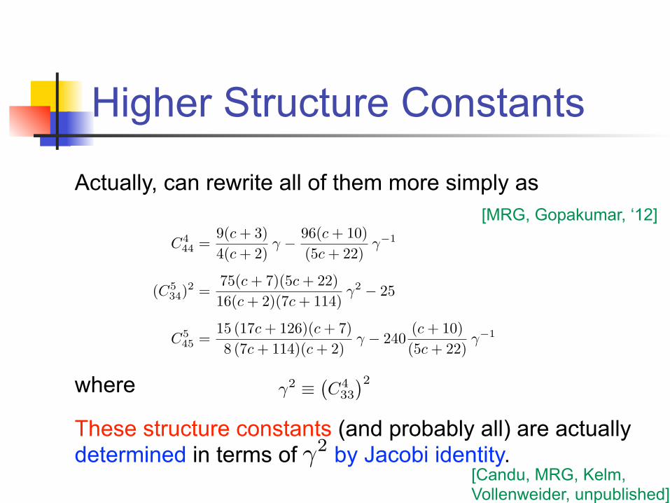
Higher Structure Constants
Actually, can rewrite all of them more simply as
where
These structure constants (and probably all) are actually determined in terms of by Jacobi identity.
[Candu, MRG, Kelm, Vollenweider, unpublished]
[MRG, Gopakumar, ‘12]
γ2

(C4
33)2 ≡ γ2 =
64(c + 2)(λ − 3)(
c(λ + 3) + 2(4λ + 3)(λ − 1))
(5c + 22)(λ − 2)(
c(λ + 2) + (3λ + 2)(λ − 1)) .
W∞[λ1] ∼= W∞[λ2] ∼= W∞[λ3] at fixed c
γ2 (rather than λ)
Quantum algebra
Thus full quantum algebra seems to be characterised by two free parameters: central charge c and
But
Thus there are three roots that lead to the same algebra:
[MRG, Gopakumar, ‘12]
`Triality’

W∞[N ] ∼= W∞[ N
N+k] ∼= W∞[− N
N+k+1] at c = cN (k)
Triality
In particular,
minimal model asymptotic symmetry algebra of hs theory
This is even true at finite N and k, not just in the ‘t Hooft limit!
This triality generalises level-rank duality of coset models of [Kuniba, Nakanishi, Suzuki, ‘91] and [Altschuler, Bauer, Saleur, ‘90].

hs[λ]
W∞[λ]
Symmetries
So the symmetries give strong evidence for the duality
HS on AdS3 2d CFT with
symmetry
=CS with
minimal models
=
(`, λ) (N, k)λ =
N
N + k
3`
4GN
= cN,ksize of AdS3 (sugra: c large)

Spectrum
Higher spin fields themselves correspond only to the vacuum representation of the W-algebra!
(Λ; 0)Contribution from all representations of the form is accounted for by adding to the hs theory a complex scalar field of mass
−1 ≤M2≤ 0 with M
2 = −(1− λ2) .
[Compatible with hs symmetry since hs theory has massive scalar multiplet with this mass.]
[Prokushkin, Vasiliev, ‘98]
[MRG, Gopakumar, ‘10]

Total 1-loop partition function
Z(1)pert =
∞∏
s=2
∞∏
n=s
1
|1− qn|2×
∞∏
l,l′=0
1
(1− qh+lq̄h+l′)2
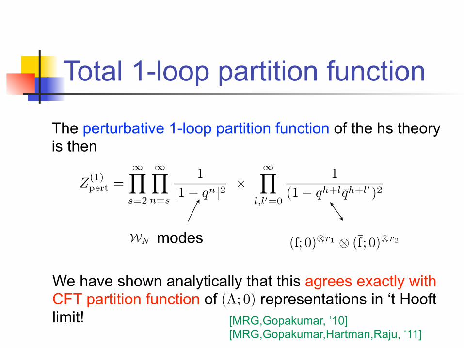
The perturbative 1-loop partition function of the hs theory is then
higher spin fields
scalar fields
Total 1-loop partition function
Z(1)pert =
∞∏
s=2
∞∏
n=s
1
|1− qn|2×
∞∏
l,l′=0
1
(1− qh+lq̄h+l′)2
The perturbative 1-loop partition function of the hs theory is then
(f; 0)⊗r1 ⊗ (̄f; 0)⊗r2modes
We have shown analytically that this agrees exactly with CFT partition function of representations in ‘t Hooft limit! [MRG,Gopakumar, ‘10]
[MRG,Gopakumar,Hartman,Raju, ‘11]
(Λ; 0)
WN

Zpert =
X
Λ
|χ(Λ,0)|2 .
Spectrum
(Λ; ν) with ν 6= 0
The remaining states, i.e. those of the form
seem to correspond to conical defect solutions (possibly dressed with perturbative excitations).
[Castro, Gopakumar, Gutperle, Raeymaekers, ‘11] [MRG, Gopakumar, ‘12] [Perlmutter, Prochazka, Raeymaekers, ‘12]
Thus

N = 4
λ =N
N + k + 2
Recent developments
In order to understand relation to string theory have studied supersymmetric version of duality, in particular, case with large superconformal symmetry.
hs theory based on
shs2[λ]Wolf space cosets
su(N + 2)k ⊕ so(4N + 4)1su(N)k+2 ⊕ u(1)κ
⊕ u(1)κ .
in ‘t Hooft limit with .
[MRG, Gopakumar, ‘13]

AdS3 × S3× S
3× S
1
Vir⊕ su(2)⊕ su(2)⊕ u(1)N = 4
Symmetries
The Wolf space coset CFTs have same symmetry as dual CFT of string theory on
with 4 supercharges
Large
[Boonstra, Peeters, Skenderis, ‘98; Elitzur, Feinerman, Giveon, Tsabar, ‘99;
de Boer, Pasquinucci, Skenderis, ‘99; Gukov, Martinec, Moore, Strominger, ‘04; ...]
N = 4
(
T4)⊗(N+1)
/SN+1
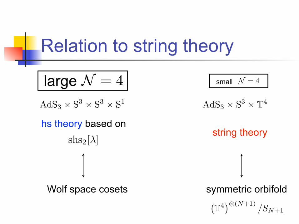
Relation to string theory
AdS3 × S3× T
4AdS3 × S
3× S
3× S
1
hs theory based on
Wolf space cosets
shs2[λ]string theory
symmetric orbifold
large N = 4small

λ =N
N + k + 2→ 0
Contraction
While we cannot compare these two dualities directly, the large superconformal symmetry contracts to the small superconformal symmetry in the limit in which the level k goes to infinity
Indeed, this just describes the case where the radius of one of the two 3-spheres goes to infinity, and hence the sphere approximates flat space.

⊂
hs theory in string theory
N = 4
AdS3 × S3× T
4AdS3 × S
3× S
3× S
1
hs theory based on
Wolf space cosets
shs2[λ]string theory
symmetric orbifold
large N = 4small
λ→0−→
SymN+1(T
4) ≡ (T4)⊗(N+1)/SN+1

su(N + 2)k ⊕ so(4N + 4)1su(N)k+2 ⊕ u(1)κ
⊕ u(1)κ .
Wolf space cosets
What happens to the Wolf space cosets in this limit?
[MRG, Suchanek, ‘11]
As in bosonic case, the `perturbative’ part of the spectrum can be identified with the U(N)-singlet sector
Hpert =M
Λ
(0; Λ)⊗ (0; Λ∗) =⇣
4(N + 1) free bosons4(N + 1) free fermions
⌘
/U(N)
[MRG, Gopakumar, ‘14]

bosons: 2 · (N,1)⊕ 2 · (N̄,1)⊕ 4 · (1,1)
fermions: (N,2)⊕ (N̄,2)⊕ 2 · (1,2)
Untwisted sector
Here the free bosons and fermions transform as
U(N) su(2)
The other coset representations can be interpreted
as twisted sectors (and descendants) of this continuous
orbifold — actually, can give very concrete identification....
[MRG, Gopakumar, ‘14] [MRG, Kelm, ‘14]

SN+1
bosons: 4 · (N+ 1,1) = 4 · (N,1)⊕ 4 · (1,1)
fermions: 2 · (N+ 1,2) = 2 · (N,2)⊕ 2 · (1,2)
Comparison
This now looks very similar to the untwisted sector of the symmetric orbifold
Indeed, this sector is generated by free bosons and fermions in
su(2)
SymN+1(T
4) ≡⇣
T4(N+1)
⌘
/SN+1

SN+1 ⊂ U(N)
Branching rule
In fact
and under this embedding, we have the branching rules
NU(N) → NSN+1N̄U(N) → NSN+1

bosons: 4 · (N,1)⊕ 4 · (1,1)
fermions: 2 · (N,2)⊕ 2 · (1,2)
Comparison
Wolf coset:
bosons: 2 · (N,1)⊕ 2 · (N̄,1)⊕ 4 · (1,1)
fermions: (N,2)⊕ (N̄,2)⊕ 2 · (1,2)
Symmetric orbifold:
Thus the action of the permutation group on the free bosons and fermions is induced from the U(N) action!

⊂
λ → 0
Subtheory
U(N) invariant states of free theory
untwisted sector of sym. orbifold
i.e. invariant states of free theory
perturbative part of CFT dual of hs theory for
(part of)
CFT dual of string theory in this limit
It therefore follows that
hs theory is closed subsector of string theory!
[MRG, Gopakumar, ‘14]
SN+1

SN+1
Stringy symmetry
From the hs point of view, the symmetric orbifold (i.e. the stringy CFT dual) is characterised by an extended chiral algebra.
multiplicity of singlet representation of
The character of this stringy algebra equals
Zstringy(q, y) =X
Λ
D(Λ)χ(0;Λ)(q, y)
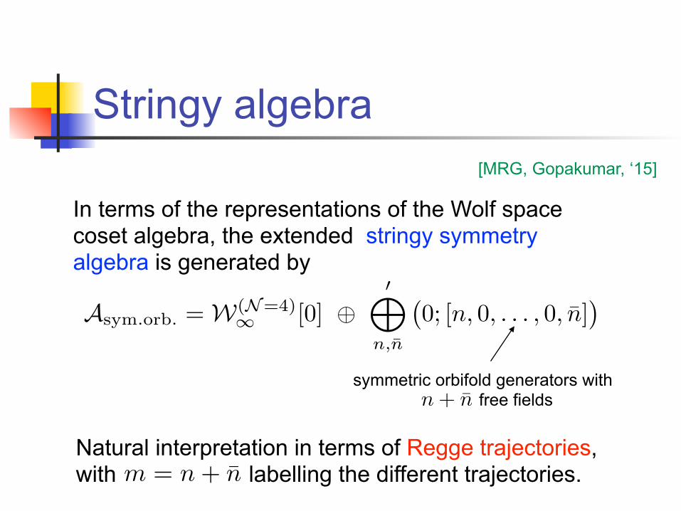
Stringy algebra
In terms of the representations of the Wolf space coset algebra, the extended stringy symmetry algebra is generated by
symmetric orbifold generators with free fields
Asym.orb. = W(N=4)1 [0] ⊕
0M
n,n̄
(
0; [n, 0, . . . , 0, n̄])
n+ n̄
Natural interpretation in terms of Regge trajectories, with labelling the different trajectories.m = n+ n̄
[MRG, Gopakumar, ‘15]

Tension perturbation
Study perturbation by exactly marginal operator that corresponds to switching on string tension — SO(4) inv. combination of moduli from 2-cycle twisted sector.
[MRG, Peng, Zadeh, ‘15]
Anomalous dimension from diagonalisation of mixing matrix
where
N (W (s)) =
bs+hΦc−1X
l=0
(−1)l
l!(L−1)
lW
(s)−s+1+l
Φperturbing
field
[Note: ] ∂z̄W(s) = g πN (W (s)) .
γij = hN (W i) , N (W j)i
cf. also [Hikida, Roenne, ‘15] [Creutzig, Hikida, ‘15]

Explicit results
spin
M2
spincubic terms
quadratic terms
Explicitly we find that
quartic terms
quintic terms
[MRG, Peng, Zadeh, ‘15]
◆ ◆ ◆ ◆ ◆ ◆ ◆ ◆ ◆ ◆◆◆◆◆◆××
××
××××
××
▲▲ ▲▲▲▲
××
×× ××××
■■ ■■ ■■
××
××××
▲▲××
1 2 3 4 5 6 7 8 9 11 13 15
1
2
3
4
56
8
10

Mixing and log behaviour
Generically, fields of the same unperturbed spin (incl. those from different columns) will mix, and the full diagonalisation problem is complicated.
[MRG, Peng, Zadeh, ‘15]
However, have good estimate for diagonal entries for the original higher spin fields,
and hence for associated dispersion relation
E(s) ' s+ a log s
γ(s)
' a log s
RR background
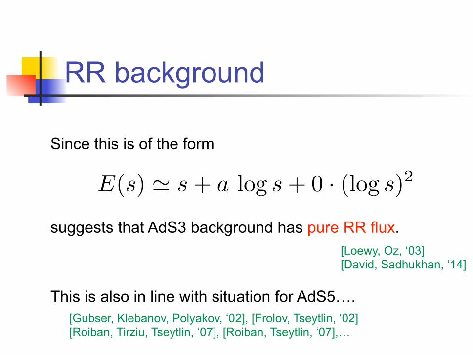
E(s) ' s+ a log s+ 0 · (log s)2
Since this is of the form
suggests that AdS3 background has pure RR flux.
[Loewy, Oz, ‘03] [David, Sadhukhan, ‘14]
This is also in line with situation for AdS5….
[Gubser, Klebanov, Polyakov, ‘02], [Frolov, Tseytlin, ‘02] [Roiban, Tirziu, Tseytlin, ‘07], [Roiban, Tseytlin, ‘07],…

λ → 0
Stringy completion
At stringy description characterised by extended chiral algebra (which could be directly obtained from symmetric orbifold).
It is natural to believe that the same idea should also work away from this special point --- this suggests a new avenue for how to find the CFT dual of string theory on
AdS3 × S3× S
3× S
1

Conclusions
‣ Explained evidence for bosonic minimal model holography and sketched large generalisation.
‣ In the supersymmetric case found natural embedding of CFT dual of hs theory into CFT dual of string theory.
‣ Gives first concrete realisation of idea that hs theory emerges as a subsector of string theory in tensionless limit.
N = 4

Open problems & future directions
HS viewpoint: new perspective on stringy CFT
‣ Find Lie algebra structure of stringy symmetry
‣ Find other stringy modular invariants
‣ higher dimensional analogue?
cf. [Beisert,Bianchi,Morales,Samtleben, ‘04]
‣ Interpretation from D1-D5 viewpoint
‣ Relation to spin chain picture
Open problems:
cf. [Chang, Minwalla, Sharma, Yin, ‘12]
[Borsato, Ohlsson Sax, Sfondrini, Stefanski, ‘14] [Babichenko, Stefanski, Zarembo, ‘09]


Interesting CFT problems
Prove that is consistent W-algebra for
all values of and c. W[λ]λ
Show that every W-algebra with this spin content
(one simple field for each spin s>1) is of this form.
Representation theory
Unitarity?
Supersymmetric generalisations, N=1, N=2, N=4.
Interesting Lie problems
Give good characterisation of stringy symmetry
algebra = wedge algebra of symmetric orbifold.
Relation to Yangian symmetry?
Representation theory
Constraints for perturbation theory via Wigner-Eckert
type argument.

Stringy chiral algebra
Explicitly, we find
This reproduces precisely vacuum character of symmetric orbifold (from DMVV).
Zstringy(q, y) = χ(0;0)(q, y) + χ(0;[2,0,...,0])(q, y) + χ(0;[0,0,...,0,2])(q, y)
+ χ(0;[3,0,...,0,0])(q, y) + χ(0;[0,0,0,...,0,3])(q, y)
+ χ(0;[2,0,...,0,1])(q, y) + χ(0;[1,0,0,...,0,2])(q, y)
+ 2 · χ(0;[4,0,...,0,0])(q, y) + 2 · χ(0;[0,0,0,...,0,4])(q, y)
+ χ(0;[0,2,0,...0,0])(q, y) + χ(0;[0,0,...0,2,0])(q, y)
+ χ(0;[3,0,...,0,1])(q, y) + χ(0;[1,0,0,...,0,3])(q, y)
+ 2 · χ(0;[2,0,0,...,0,2])(q, y) + · · ·

Light States
The stringy extension does not contain any of the `light’ states any longer since they do not give rise to allowed (untwisted) representations of the extended chiral algebra.
Spacetime intepretation: classical hs solutions do not all lift to string theory.


