
High Fidelity Readout
and Protection
of a 43Ca+ Trapped Ion Qubit
A thesis submitted for the degree of
Doctor of Philosophy
0 5 10 15 20 25 30 35 40 450
0.1
0.2
0.3
0.4
0.5
0.6
0.7
0.8
0.9
1
τ / ms
Fri
nge C
on
tra
st (
not
norm
ali
sed
)
0
1
1
3
5
6
6
6
10
20
20
No. of π pulses
David Szwer
Trinity Term
2009
St. Catherine’s College
Oxford


Abstract
High Fidelity Readout and Protection of a 43Ca+ Trapped Ion Qubit
A thesis submitted for the degree of Doctor of Philosophy
Trinity Term 2009
David Szwer
St. Catherine’s College, Oxford
This thesis describes theoretical and experimental work whose main aim is the develop-
ment of techniques for using trapped 43Ca+ ions for quantum information processing.
I present a rate equations model of 43Ca+, and compare it with experimental data.
The model is then used to investigate and optimise an electron-shelving readout method
from a ground-level hyperfine qubit. The process is robust against common experimental
imperfections. A shelving fidelity of up to 99.97% is theoretically possible, taking 100 µs.
The laser pulse sequence can be greatly simplified for only a small reduction in the
fidelity. The simplified method is tested experimentally with fidelities up to 99.8%. The
shelving procedure could be applied to other commonly-used species of ion qubit.
An entangling two-qubit quantum controlled-phase gate was attempted between a
40Ca+ and a 43Ca+ ion. The experiment did not succeed due to frequent decrystallisation
of the ion pair, and strong motional decoherence. The source of the problems was never
identified despite significant experimental effort, and the decision was made to suspend
the experiments and continue them in an improved ion trap which is under construction.
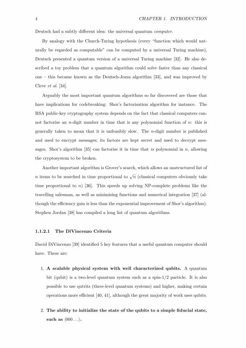
A sequence of π-pulses, inspired by the Hahn spin-echo, was derived that is capable
of greatly reducing dephasing of any qubit. If the qubit precession frequency varies with
time as an nth-order polynomial, an (n + 1) pulse sequence is theoretically capable of
perfectly cancelling the resulting phase error. The sequence is used on a 43Ca+ magnetic-
field-sensitive hyperfine qubit, with 20 pulses increasing the coherence time by a factor of
75 compared to an experiment without any spin-echo. In our ambient noise environment
the well-known Carr-Purcell-Meiboom-Gill dynamic-decoupling method was found to be
comparably effective.

Acknowledgements
A great many thanks are due to Dr. David Lucas, my supervisor. Without him this
work would not have been possible, and not just because he was the man with the
grant. His confidence and enthusiasm for all things ion, together with encyclopaedic
knowledge of the experiment, carried me through where guidance and inspiration alone
may have failed. This thesis is also grateful for his proofreading skills and helpful textual
suggestions. Many thanks to Prof. Andrew Steane for many useful conversations, and
to him and David for doing all the behind-the-scenes work that keeps the group going.
I must also thank Prof. Derek Stacey very much for his enviably deep understanding of
atomic physics, and his insatiable appetite for fittable scans.
To the rest of Team Ion: thank you. Both the past members (Dr. Paul Barton,
Dr. Charles Donald, Dr. Angel Ramos, Dr. Marek Sasura, Dr. John-Patrick Stacey, Dr.
David Stevens and Dr. Simon Webster) and the ones I have worked with (David Allcock,
Michael Curtis, Dr. Jonathan Home, Dr. Gergely Imreh, Dr. Ben Keitch, Norbert Linke,
Dr. Matt McDonnell, Alice Burrell, Dr. Eoin Phillips, Dr. Jeff Sherman, Dr. Nicholas
Thomas and Dr. Simon Webster again) have done so much to build up the apparatus into
the intricate physics machine it is today. Your moral and technical support have been
invaluable these past four years. Special mentions go to Gergely, Alice and Simon for
respectively being my ICAP, readout and lab buddies. Thanks also to Graham Quelch
for his help with electronics and other practical matters; and Rob Harris for making any
visit to the workshop a pleasure.
Thanks to all my friends in both halves of Oxbridge. They’ve given me a lot of fun
over the years, and I wouldn’t have been able to stay in the lab if I hadn’t known there
was a friendly world waiting for me outside it.
Finally, without the constant love and support of my family, especially my parents,
I would never have made it this far. I can never thank them enough.

vi ACKNOWLEDGEMENTS

Contents
Abstract iii
Acknowledgements v
1 Introduction 1
1.1 Background . . . . . . . . . . . . . . . . . . . . . . . . . . . . . . . . . . 1
1.1.1 Ion Trapping . . . . . . . . . . . . . . . . . . . . . . . . . . . . . 1
1.1.1.1 Laser-Based Studies . . . . . . . . . . . . . . . . . . . . 1
1.1.1.2 Laser-Free Studies . . . . . . . . . . . . . . . . . . . . . 2
1.1.2 Quantum Computing . . . . . . . . . . . . . . . . . . . . . . . . 3
1.1.2.1 The DiVincenzo Criteria . . . . . . . . . . . . . . . . . 4
1.1.2.2 Decoherence and Error Correction . . . . . . . . . . . . 5
1.1.2.3 Implementations . . . . . . . . . . . . . . . . . . . . . . 6
1.1.3 Quantum Computing with Trapped Ions . . . . . . . . . . . . . . 7
1.1.3.1 DiVincenzo Criteria applied to Trapped Ions . . . . . . 7
1.1.3.2 Other Progress with Trapped Ions . . . . . . . . . . . . 11
1.1.3.3 Scaling up . . . . . . . . . . . . . . . . . . . . . . . . . 12
1.2 Structure of this Thesis . . . . . . . . . . . . . . . . . . . . . . . . . . . 13
2 Apparatus 15
2.1 Calcium . . . . . . . . . . . . . . . . . . . . . . . . . . . . . . . . . . . . 15
2.1.1 Notation . . . . . . . . . . . . . . . . . . . . . . . . . . . . . . . . 15
2.1.2 Levels and Transitions . . . . . . . . . . . . . . . . . . . . . . . . 16
2.2 Trapping Ions . . . . . . . . . . . . . . . . . . . . . . . . . . . . . . . . . 17
2.2.1 Tickling . . . . . . . . . . . . . . . . . . . . . . . . . . . . . . . . 19
2.2.2 Loading . . . . . . . . . . . . . . . . . . . . . . . . . . . . . . . . 21
vii
viii CONTENTS
2.2.3 Vacuum . . . . . . . . . . . . . . . . . . . . . . . . . . . . . . . . 22
2.3 Computer Control . . . . . . . . . . . . . . . . . . . . . . . . . . . . . . 22
2.3.1 Laser Control Unit . . . . . . . . . . . . . . . . . . . . . . . . . . 24
2.4 Lasers . . . . . . . . . . . . . . . . . . . . . . . . . . . . . . . . . . . . . 24
2.4.1 Summary of Lasers . . . . . . . . . . . . . . . . . . . . . . . . . . 24
2.4.2 Beam Geometry and Polarisations . . . . . . . . . . . . . . . . . 25
2.4.3 Diagnostics . . . . . . . . . . . . . . . . . . . . . . . . . . . . . . 25
2.4.3.1 Frequency Diagnostics . . . . . . . . . . . . . . . . . . . 25
2.4.3.2 Intensity Diagnostics . . . . . . . . . . . . . . . . . . . 27
2.4.4 Locking . . . . . . . . . . . . . . . . . . . . . . . . . . . . . . . . 28
2.4.5 Switching and Fine Frequency Control . . . . . . . . . . . . . . . 29
2.4.6 Laser-Specific Details . . . . . . . . . . . . . . . . . . . . . . . . 30
2.4.6.1 397D40 and 397D43 . . . . . . . . . . . . . . . . . . . . 30
2.4.6.2 397 Master/Slave . . . . . . . . . . . . . . . . . . . . . 31
2.4.6.3 393 . . . . . . . . . . . . . . . . . . . . . . . . . . . . . 31
2.4.6.4 866 . . . . . . . . . . . . . . . . . . . . . . . . . . . . . 31
2.4.6.5 854Old and 854New . . . . . . . . . . . . . . . . . . . . 31
2.4.6.6 850 . . . . . . . . . . . . . . . . . . . . . . . . . . . . . 32
2.5 Coherent Manipulation . . . . . . . . . . . . . . . . . . . . . . . . . . . . 32
2.5.1 Magnetic Resonance . . . . . . . . . . . . . . . . . . . . . . . . . 32
2.5.2 Raman Transitions . . . . . . . . . . . . . . . . . . . . . . . . . . 33
2.5.3 Microwave Transitions . . . . . . . . . . . . . . . . . . . . . . . . 33
2.5.4 Synthesiser Network . . . . . . . . . . . . . . . . . . . . . . . . . 34
2.6 Imaging System . . . . . . . . . . . . . . . . . . . . . . . . . . . . . . . . 36
2.7 Ancillary Experiments . . . . . . . . . . . . . . . . . . . . . . . . . . . . 40
2.7.1 AOM Extinction . . . . . . . . . . . . . . . . . . . . . . . . . . . 40
2.7.1.1 RF Extinction of 850 nm AOM . . . . . . . . . . . . . . 40
2.7.1.2 Extinction of 397 nm beams . . . . . . . . . . . . . . . . 41
2.7.2 850 Polarisation . . . . . . . . . . . . . . . . . . . . . . . . . . . 44
3 Rate Equations 51
3.1 Basic Atomic Theory . . . . . . . . . . . . . . . . . . . . . . . . . . . . . 51
3.1.1 Rate Equations . . . . . . . . . . . . . . . . . . . . . . . . . . . . 51

CONTENTS ix
3.1.2 Forming M . . . . . . . . . . . . . . . . . . . . . . . . . . . . . . 53
3.1.2.1 Electric Dipole Transitions (E1) . . . . . . . . . . . . . 54
3.1.2.2 Electric Multipole Transitions . . . . . . . . . . . . . . 55
3.1.2.3 Magnetic Dipole Transitions (M1) . . . . . . . . . . . . 58
3.1.3 Hyperfine Energy Shifts . . . . . . . . . . . . . . . . . . . . . . . 59
3.2 The Transitions Suite . . . . . . . . . . . . . . . . . . . . . . . . . . . . 60
3.3 Atomic Constants . . . . . . . . . . . . . . . . . . . . . . . . . . . . . . 60
3.4 Simulations of Ion Fluorescence in 43Ca+ . . . . . . . . . . . . . . . . . 63
3.4.1 Bloch Equations . . . . . . . . . . . . . . . . . . . . . . . . . . . 69
3.4.2 397 nm, 850 nm and 854 nm Fluorescence . . . . . . . . . . . . . 71
3.5 Simulations of Far Off-Resonance . . . . . . . . . . . . . . . . . . . . . . 72
3.5.1 Effect on 43Ca+ of 397 nm radiation tuned to 40Ca+ . . . . . . . 72
3.5.2 Shelving Effect on 40Ca+ of 397 nm and 866 nm Light . . . . . . 73
3.5.3 Deshelving Effect on 40Ca+ of 850 nm and 866 nm . . . . . . . . 75
3.5.3.1 43Ca+ . . . . . . . . . . . . . . . . . . . . . . . . . . . . 75
3.6 Simulations of Optical Pumping into 43Ca+ Clock States . . . . . . . . . 77
4 Readout 81
4.0.1 Notation . . . . . . . . . . . . . . . . . . . . . . . . . . . . . . . . 83
4.1 Shelving 43Ca+ . . . . . . . . . . . . . . . . . . . . . . . . . . . . . . . . 84
4.1.1 Multi-pulse Shelving . . . . . . . . . . . . . . . . . . . . . . . . . 84
4.1.2 Single Pulse Shelving . . . . . . . . . . . . . . . . . . . . . . . . . 85
4.2 Optimisation Simulations . . . . . . . . . . . . . . . . . . . . . . . . . . 86
4.2.1 Optimisation Methods . . . . . . . . . . . . . . . . . . . . . . . . 87
4.2.2 Optimum Fidelity as a Function of Time . . . . . . . . . . . . . 91
4.2.2.1 Multi-pulse . . . . . . . . . . . . . . . . . . . . . . . . . 91
4.2.2.2 Single Pulse, Multiple 850 nm Beams . . . . . . . . . . 98
4.2.2.3 Single Pulse, Single 850 nm Beam . . . . . . . . . . . . 98
4.2.2.4 Clock States . . . . . . . . . . . . . . . . . . . . . . . . 107
4.2.2.5 Summary . . . . . . . . . . . . . . . . . . . . . . . . . . 107
4.2.3 Fidelity as a Function of Parameters . . . . . . . . . . . . . . . . 107
4.3 Experiments . . . . . . . . . . . . . . . . . . . . . . . . . . . . . . . . . . 118
4.3.1 850 nm Parallel to Magnetic Field . . . . . . . . . . . . . . . . . 118

x CONTENTS
4.3.2 850 nm at Small Angle to Magnetic Field . . . . . . . . . . . . . 119
4.3.2.1 Various Results . . . . . . . . . . . . . . . . . . . . . . 119
4.3.2.2 Population-Preparation Improvement . . . . . . . . . . 120
4.3.2.3 Some Trends . . . . . . . . . . . . . . . . . . . . . . . . 124
4.3.2.4 Effect of λ4 Waveplate Rotation . . . . . . . . . . . . . . 124
4.3.2.5 The Best Results . . . . . . . . . . . . . . . . . . . . . . 126
4.4 Future Directions . . . . . . . . . . . . . . . . . . . . . . . . . . . . . . . 129
4.5 Comparison with the Literature . . . . . . . . . . . . . . . . . . . . . . . 130
5 40-43 133
5.1 Introduction . . . . . . . . . . . . . . . . . . . . . . . . . . . . . . . . . . 134
5.1.1 Light-Motion Interaction . . . . . . . . . . . . . . . . . . . . . . 134
5.1.1.1 Resolved Sideband Interactions and Cooling . . . . . . 134
5.1.1.2 Optical Dipole Force . . . . . . . . . . . . . . . . . . . . 136
5.1.1.3 Same-Species Gate . . . . . . . . . . . . . . . . . . . . . 137
5.1.1.4 Mixed-Species Gate . . . . . . . . . . . . . . . . . . . . 139
5.1.2 Mixed-Isotope Readout . . . . . . . . . . . . . . . . . . . . . . . 139
5.1.3 Pulse Sequence . . . . . . . . . . . . . . . . . . . . . . . . . . . . 141
5.2 Crystal issues and Ion Ejection . . . . . . . . . . . . . . . . . . . . . . . 144
5.2.1 Crystallisation . . . . . . . . . . . . . . . . . . . . . . . . . . . . 144
5.2.2 Ion Ejection . . . . . . . . . . . . . . . . . . . . . . . . . . . . . . 145
5.3 Electrode Noise and RF Harmonics . . . . . . . . . . . . . . . . . . . . . 146
5.3.1 RF Correlation . . . . . . . . . . . . . . . . . . . . . . . . . . . . 146
5.3.2 RF Harmonics . . . . . . . . . . . . . . . . . . . . . . . . . . . . 147
5.3.3 Electrode Noise . . . . . . . . . . . . . . . . . . . . . . . . . . . . 147
5.4 Raman Motional Spectra . . . . . . . . . . . . . . . . . . . . . . . . . . 151
5.4.1 Observation of Radial Mode in Axial Raman Scans . . . . . . . . 151
5.4.2 Heating Rates . . . . . . . . . . . . . . . . . . . . . . . . . . . . . 151
5.4.3 Motional Coherence . . . . . . . . . . . . . . . . . . . . . . . . . 154
5.4.4 Schrodinger Cats . . . . . . . . . . . . . . . . . . . . . . . . . . . 155
5.5 Conclusion . . . . . . . . . . . . . . . . . . . . . . . . . . . . . . . . . . 157
6 Dynamic Decoupling 161
6.1 Theory . . . . . . . . . . . . . . . . . . . . . . . . . . . . . . . . . . . . . 162
CONTENTS xi
6.2 Proof that the UDD Sequence Solves the Equations . . . . . . . . . . . 165
6.2.1 A Lemma . . . . . . . . . . . . . . . . . . . . . . . . . . . . . . . 165
6.2.2 Useful Results . . . . . . . . . . . . . . . . . . . . . . . . . . . . 167
6.2.3 The Proof . . . . . . . . . . . . . . . . . . . . . . . . . . . . . . . 168
6.2.4 Optimality . . . . . . . . . . . . . . . . . . . . . . . . . . . . . . 170
6.3 The Literature . . . . . . . . . . . . . . . . . . . . . . . . . . . . . . . . 171
6.3.1 Theory . . . . . . . . . . . . . . . . . . . . . . . . . . . . . . . . 171
6.3.2 Experiment . . . . . . . . . . . . . . . . . . . . . . . . . . . . . . 172
6.4 Our Experiment . . . . . . . . . . . . . . . . . . . . . . . . . . . . . . . 174
6.4.1 AC Field Compensation . . . . . . . . . . . . . . . . . . . . . . . 174
6.4.2 Spin-Echo Sequences . . . . . . . . . . . . . . . . . . . . . . . . . 179
6.4.2.1 Conclusions . . . . . . . . . . . . . . . . . . . . . . . . . 183
7 Conclusion 189
7.1 Future Developments . . . . . . . . . . . . . . . . . . . . . . . . . . . . . 191
A Hyperfine Structure of 43Ca+ 193
B The Transitions Suite: Users’ Guide 197
B.1 Setting Up . . . . . . . . . . . . . . . . . . . . . . . . . . . . . . . . . . . 197
B.2 Adding and Using Lasers . . . . . . . . . . . . . . . . . . . . . . . . . . 198
B.3 Solving . . . . . . . . . . . . . . . . . . . . . . . . . . . . . . . . . . . . . 199
B.4 Utility Functions . . . . . . . . . . . . . . . . . . . . . . . . . . . . . . . 200
B.5 Example . . . . . . . . . . . . . . . . . . . . . . . . . . . . . . . . . . . . 201

xii CONTENTS

“Taking the attitude that the pursuit of as basic an ideal as a single
atomic particle at rest in space is a thoroughly worthwhile intellectual
endeavor we are undertaking experiments along these lines.”
Neuhauser, Hohenstatt, Toschek and Dehmelt [12]
Chapter 1
Introduction
1.1 Background
1.1.1 Ion Trapping
In 1979, not many decades since the very existence of atoms was a matter for debate
[1, 2], a team at Heidelberg University isolated and observed a single Ba+ ion [3].
Suspended by radio-frequency electric fields in a vacuum, illuminated by lasers and
laser-cooled to a few tens of millikelvin, such an atom is almost entirely free of the
influence of other matter and thus provides an ideal laboratory for testing fundamental
physical theories. The history of ion trapping goes back further, to Fischer’s trap of
1959 [4] and the quadrupole mass filter (essentially a linear Paul trap, like our own, but
with no endcaps) that was first used for mass-spectroscopy in 1955 by Paul and Raether
[5, 6]. But it is the ability to isolate individual atoms that makes the field so exciting
today.
As well as the all-electric Paul traps (in various geometries) many experiments are
performed with Penning traps, which use constant magnetic and electric fields to trap
orbiting ions. Dehmelt and Paul won (half of) the 1989 Nobel Prize for Physics for
inventing the Penning and Paul traps [7].
1.1.1.1 Laser-Based Studies
One major motivation for developing ion-trap technology is its potential for use in the
next generation of atomic clocks. Current caesium fountain clocks boast frequency
uncertainties of less than 10−15 [8], but only after about one day of averaging. This
1

2 CHAPTER 1. INTRODUCTION
is because they are based on a microwave transition at 9.2 GHz; a clock based on an
optical transition at ∼ 1014−1015 Hz could reach a similar level in just a few seconds. A
trapped ion is almost ideal as such an optical frequency standard: with extremely good
isolation, cooling to the ground state of motion and long interrogation time, Wineland
et al. say, “...it does not seem unreasonable to think that accuracies and measurement
precisions at or beyond 1 part in 1018 will be achieved” [9]. An example of progress is
that the ratio of two ultraviolet transitions, in 199Hg+ and 27Al+, has been measured
to a fractional uncertainty of 5.2 × 10⁻¹⁷ by Rosenband et al. [10]; many other projects
are underway using different ions [11, Section 3 and references therein].
Although not yet mature enough to provide a new definition of the second, optical
clock research is already producing results in fundamental physics. Frequency ratios,
such as that by Rosenband et al. above, depend on the fine structure constant α. By
repeatedly measuring the ratio over a period of time, changes in α could be detected
that are predicted by various theories beyond the standard model [13]. The first ion-
based measurement is by Rosenband et al. who deduce a (provisional) limit of αα =
−1.6(2.3) × 10−17 [10], consistent with zero and competitive with other bounds from,
for instance, the Oklo natural nuclear reactor [13].
Detailed quantum-mechanical calculation methods, such as multiconfiguration
Hartree-Fock [14], can be tested by calculating and measuring properties of trapped
ions. Excited state lifetimes [14, 15], isotope shifts and hyperfine structure [16] and gy-
romagnetic ratios [17] have all been used; ratios of light shifts of different levels of an ion
have been measured [18, 19] but not yet calculated. Such measurements, as well as mea-
suring transition frequencies, are also useful for calibrating astronomical observations
[20, 21].
Experiments have been proposed to measure parity non-conservation in trapped ions,
often Ba+ or Ra+. Studying violation of parity symmetry could both test the standard
model, even measuring the mass of the Higgs boson, and reveal new physics such as
supersymmetry [22, 23].
1.1.1.2 Laser-Free Studies
By forcing an ion to perform orbits, principally at the cyclotron frequency that is in-
versely proportional to its mass, a Penning trap can be used as an accurate and precise
mass spectrometer. One team in this area is the SMILETRAP group at Stockholm
1.1. BACKGROUND 3
University, which has weighed numerous ions to relative uncertainties below 10−9. Mea-
suring the masses of 3He and 3H gives the tritium β-decay energy which is needed for
measurements of the electron antineutrino mass; masses of silicon isotopes could con-
tribute to a redefinition of the kilogramme based on atomic quantities; masses of 76Ge
and 76Se help in the search for neutrinoless double β-decay which would violate the
standard model; and the mass of 133Cs allows a calculation of α (because the photon
recoil of caesium atoms has been measured [24]) [25].
A similar technique has been used with antimatter. The TRAP collaboration (and
later, ATRAP) at CERN has operated a succession of Penning traps over ten years, mea-
suring the relative masses of protons and antiprotons, and improving the experimental
precision by a millionfold over that time to show they are approximately equal to 90
parts-per-trillion [26]. The gyromagnetic ratio g ≈ 2 has been measured in electrons
and positrons, providing further tests of fundamental physics [27, 28].
1.1.2 Quantum Computing
Richard Feynman gave a keynote address at the 1981 MIT Physics of Computation
conference, and created a new area of physics [29]. He proposed a universal quantum
simulator – a quantum system that could simulate or calculate the behaviour of any
other system – and argued that such a thing was needed because the state space of an
interesting quantum system is in some senses too large for normal, classical computers.
For instance, suppose one wants to simulate a set of n interacting particles, each of
which can be in two states |1〉 or |0〉. For classical particles, we would simply choose
one of the 2n possible starting states and perform the simulation, and the problem
reduces to some kind of numerical integration or similar. But quantum particles can be
in superpositions such as (|1〉 + |2〉) /√
2, and the phenomenon of entanglement means
that the superposition must be considered over the system as a whole, rather than for
each particle individually. Thus the calculation must work with all of the 2n states of
the system: adding one extra particle doubles the calculation time.
Feynman believed the only solution was a computer that also played by quantum
rules: that harnessed the massive parallelism provided by superposition and entangle-
ment, and efficiently simulated quantum problems by scaling as fast as the problems
did. He didn’t know whether a universal quantum simulator was possible, and it wasn’t
shown to be true until Seth Lloyd proved it in 1996 [30, 31]. But in the meantime David
4 CHAPTER 1. INTRODUCTION
Deutsch had a subtly different idea: the universal quantum computer.
By analogy with the Church-Turing hypothesis (every “function which would nat-
urally be regarded as computable” can be computed by a universal Turing machine),
Deutsch presented a quantum version of a universal Turing machine [32]. He also de-
scribed a toy problem that a quantum algorithm could solve faster than any classical
one – this became known as the Deutsch-Jozsa algorithm [33], and was improved by
Cleve et al. [34].
Arguably the most important quantum algorithms so far discovered are those that
have implications for codebreaking: Shor’s factorisation algorithm for instance. The
RSA public-key cryptography system depends on the fact that classical computers can-
not factorise an n-digit number in time that is any polynomial function of n: this is
generally taken to mean that it is unfeasibly slow. The n-digit number is published
and used to encrypt messages; its factors are kept secret and used to decrypt mes-
sages. Shor’s algorithm [35] can factorise it in time that is polynomial in n, allowing
the cryptosystem to be broken.
Another important algorithm is Grover’s search, which allows an unstructured list of
n items to be searched in time proportional to√
n (classical computers obviously take
time proportional to n) [36]. This speeds up solving NP-complete problems like the
travelling salesman, as well as minimising functions and numerical integration [37] (al-
though the efficiency gain is less than the exponential improvement of Shor’s algorithm).
Stephen Jordan [38] has compiled a long list of quantum algorithms.
1.1.2.1 The DiVincenzo Criteria
David DiVincenzo [39] identified 5 key features that a useful quantum computer should
have. These are:
1. A scalable physical system with well characterized qubits. A quantum
bit (qubit) is a two-level quantum system such as a spin-1/2 particle. It is also
possible to use qutrits (three-level quantum systems) and higher, making certain
operations more efficient [40, 41], although the great majority of work uses qubits.
2. The ability to initialize the state of the qubits to a simple fiducial state,
such as |000 . . .〉.
1.1. BACKGROUND 5
3. Long relevant decoherence times, much longer than the gate operation
time.
4. A “universal” set of quantum gates. The general rule is that one must be
able to apply arbitrary single-qubit gates (rotations by any angle about any axis,
which can of course be synthesized from as few as two rotations), and at least one
two-qubit gate such as controlled-NOT or controlled-Z (in which a NOT gate or
a phase rotation, respectively, is applied to one qubit if-and-only-if the second,
control qubit is in state |1〉). A quantum computer might be more efficient if a
wider variety of gates (such as controlled-NOT with more than one control qubit)
is possible.
5. A qubit-specific measurement capability.
1.1.2.2 Decoherence and Error Correction
A classical computer has a negligible error rate for its fundamental operations, but
quantum computers will probably be much less robust. Peter Shor and Andrew Steane
independently developed quantum error correction: a set of subtle techniques for sep-
arating the error from the computer’s state, so that the error can be measured and
corrected without disturbing the delicate superpositions and entanglements of the state
itself. Nielsen and Chuang [42] has a detailed account of the subject.
The basic idea is to encode a single logical qubit (a |0〉+b |1〉) in several logical qubits.
The simplest scheme, for example, “copies”1 one logical qubit onto three physical qubits
a |0〉 + b |1〉 → a |000〉 + b |111〉. After being stored for a time, or transmitted along a
noisy channel, the encoding process is repeated and two of the qubits are measured.
The measurements obtained tell us whether or not one of the qubits was flipped, and
which one it was. This allows us to correct the remaining qubit if necessary, and restore
the original state. This scheme can only correct single bit-flip errors, but it is possible
to make more complex codes that can correct any general error, even complete loss of a
physical qubit.
Fault-tolerant quantum computing extends error-correction to the quantum gates.
1Of course, it is impossible to truly copy a qubit. (a |0〉 + b |1〉) |0〉 → (a |0〉 + b |1〉) (a |0〉 + b |1〉) is
banned by the no-cloning theorem ([43, 44] and [42, Box 12.1]); but (a |0〉 + b |1〉) |0〉 → (a |00〉 + b |11〉)
can be done, and is the basis of quantum error correction.

6 CHAPTER 1. INTRODUCTION
The logical qubits remain encoded throughout the computation, and each logical gate is
made up of many physical gates. The error rate of the logical gates can be made as low
as desired, provided that the physical-gate error probability is below some threshold.
The threshold is typically estimated to be around 10−4, well below the error rate of
current experimental gates.
1.1.2.3 Implementations
Numerous physical systems have been proposed for implementing quantum computing
(QC). Trapped ions are, of course, the main subject of this thesis and will be considered
separately. Other important systems include nuclear magnetic resonance (NMR), using
the spins of nuclei in (usually liquid) molcules as qubits. An NMR machine has used a
7-qubit molecule to perform Shor’s algorithm and factorise 15 [45], the largest number
of qubits so far used in any quantum algorithm. However there are doubts about its
ability to scale to larger processors [46].
Photons having, say, two orthogonal polarisation states, have been used as qubits,
with two groups having demonstrated 2-qubit Grover searches [47, 48]. Most QC propos-
als use the “circuit model”, where quantum gates, measurements etc. are consecutively
applied to the qubits. This turns out to be highly inefficient with photons because they
can only be entangled with a small probability [49]. Instead, the Grover implementa-
tions used “one-way” quantum computing: photons were created in a specific entangled
“cluster” state, and then the algorithm was performed just by measuring the photons
(carefully choosing which photons to measure, and in what basis). A recent review of
one-way QC is by Briegel et al. [50].
Solid-state systems, such as quantum dots in semiconductors or superconducting
circuits, are very attractive in terms of being potentially highly scalable. However,
they currently have very high decoherence rates. Recently a two-qubit superconducting
processor was used to perform the Deutsch-Jozsa and Grover’s algorithms [51].
There are also ideas such as topological QC, in which quasiparticle “anyons” are
moved around each other to perform gates that could be highly resistant to errors [52];
or adiabatic quantum computing, in which a Hamiltonian is slowly altered so that the
final ground state encodes the solution to the problem [53].

1.1. BACKGROUND 7
1.1.3 Quantum Computing with Trapped Ions
Ion trapping is one of the most advanced and promising implementations of quantum
computing. It is advanced because most of the DiVincenzo criteria have been demon-
strated, along with some simple algorithms; and it is promising because there is much
progress being made towards scaling up to a full scale computer, and reducing error rates
below the error-correction threshold. Haffner, Roos and Blatt have recently published
a comprehensive review of the subject [54].
1.1.3.1 DiVincenzo Criteria applied to Trapped Ions
A scalable physical system with well characterized qubits. A qubit is stored in
two Zeeman states of an ion’s ground energy level (using the electron’s spin); or in two
hyperfine-split levels (using the combined nuclear and electron spins); or in two energy
levels separated by an optical-frequency transition. Optical qubits have the disadvantage
that the upper level usually has a significant decay rate (e.g. 1/1.17 s for a qubit in the
S1/2 and D5/2 levels of Ca+ [55]), setting a hard limit to the coherence time.
If an ion has hyperfine structure, it is possible to choose two qubit states whose
separation becomes independent of the magnetic field (to first order) at some choice of
magnetic field. These are often called “clock states” because of their obvious application
in atomic clocks. Such a qubit is highly resistant to magnetic field noise. The states can
be in the ground level, or separated by an optical transition.
The ability to initialize the state of the qubits to a simple fiducial state,
such as |000 . . .〉. Ion qubits are easy to initialise by optical pumping – illuminating
the ion with light of a single polarisation or frequency so that the ion enters a dark
state. A naıve method, such as simply using polarised light, may not be able to reach
the fault-tolerance threshold (in that case, because even small amounts of polarisation
impurity can significantly reduce the fidelity). 99.9% accurate state preparation was
achieved by the Innsbruck ion-trap group by exploiting the frequency selectivity of a
narrow quadrupole transition [56].
Long relevant decoherence times, much longer than the gate operation time.
Qubits stored in ground-level clock states can have very long coherence times. In 171Yb+,
a T2 (phase-coherence) time of 2.5(3) s was measured [57], while our group used 43Ca+
8 CHAPTER 1. INTRODUCTION
and could detect no decoherence over 1 s [58]. Both experiments used spin-echo pulses
to compensate for static errors in the qubit frequency (Langer et al. [59] achieved T2 =
14.7(1.6) s in 9Be+ even without a spin-echo). In the extremely stable field of a Penning
trap, coherence times of several minutes have been observed [60] (the other experiments
were in Paul traps). These times are far longer than current experimental gate times
of 10−5-10−4 s (see below). As technology improves it seems very likely that gates will
get faster (as motional frequencies of traps increase) and coherence times longer (as
magnetic field stabilisation improves, or high-field clock states are used).
A “universal” set of quantum gates. Single-qubit gates seem straightforward:
a coherent pulse of laser light, microwaves or radio waves are applied to drive Rabi
oscillations between the qubit states. The difficulty comes with individually addressing
ions that may be separated by just a few µm. If using lasers, the beams can be tightly
focused on the ions; the ion spacing can be increased during certain portions of the
algorithm to make this easier [61, 62]. Longer-wavelength radiation cannot be focused so
the ions must be distinguished in frequency space, either by a magnetic field gradient [63,
64] or by using a laser beam to selectively light-shift a certain ion [65]. In a microtrap,
it may be possible to use DC voltages on the segmented electrodes to push selected ions
radially so that they experience micromotion; the resulting sidebands allow a laser to
selectively address them despite illuminating all ions in the string [66].
Multi-qubit gates (almost always two-qubit) require the ions to be coupled by a
“bus”: a single quantum mode that the ions can couple to in a controlled manner. In
most cases, two ions interact via their Coulomb repulsion and share a motional mode.
Lasers are used to state-selectively couple the ions to the mode, and the bus mediates a
phase shift or bit-flip.
There are three common two-qubit gates. The Cirac-Zoller gate was the first to be
invented [67] (effectively initiating the field of trapped ion QC), and the core steps were
experimentally demonstrated the same year [68]. One of the qubits is directly mapped
to the motional mode using a sideband π-pulse. The second qubit is then driven around
a complete 2π Rabi oscillation with some auxiliary energy state, this pulse being tuned
so that it only occurs if the ions’ motion is excited, and the ions pick up a differential
phase shift of π. Then another sideband pulse on the first ion undoes the motional
excitation. The upshot is a two-qubit phase gate, enough for universal QC. Cirac-Zoller
1.1. BACKGROUND 9
gates (with a modification to the 2π step) have been performed with 92.6(6)% fidelity at
Innsbruck [69] using optical qubits in 40Ca+, each gate taking 500 µs. The Cirac-Zoller
gate requires single-ion addressing and good ground-state cooling of the motional mode.
A Mølmer-Sørenson gate [70] is much less sensitive to the motional mode’s temper-
ature and does not need single-ion addressing. Two laser beams illuminate the ions
equally such that the light’s sum frequency is twice the qubit splitting, but with each
individual beam tuned close to (but not resonant with) a motional sideband (one to a red
sideband, the other to a blue). The effect is to produce Rabi oscillations of the collective
two-qubit state, and this leads to a universal two-qubit gate. Innsbruck have used this
gate to entangle two 40Ca+ optical qubits, with a fidelity of 99.3(1)% and a gate time
of 50 µs [71]; and also two 43Ca+ optical clock states, with a fidelity of 96.9(3)% and a
gate time of 100 µs [72]. The ion-trap group at the University of Michigan have created
all four Bell states with average fidelity 79% and a gate time of 80 µs [65]; they used
clock-state hyperfine qubits in 111Cd+.
The third common gate, called a “geometric phase gate” or “wobble gate”, is a vari-
ant of Mølmer-Sørenson – whereas the Mølmer-Sørenson gate minimises the excitation
of the motional mode at all times, the wobble gate causes a large motional excitation
but minimises its effect on the (populations of the) qubit states. The lasers are used to
apply a state-dependent force to the ions that forces them into a wobbling motion, as
the name suggests, and that motion causes a phase shift. I give a longer description in
section 5.1. The gate was first described and implemented by the National Institute of
Standards and Technology (NIST) in Boulder, Colorado. They produced an entangled
Bell state with 97% fidelity in 9Be+ hyperfine qubits [73], with a gate time of 39 µs. Our
group has achieved 83% fidelity with 40Ca+ Zeeman qubits [74, 75], using a gate time
of 88 µs. Wobble gates have the same advantages as Mølmer-Sørenson gates, and could
also be performed faster for a given fidelity. However the standard wobble gate will not
work with clock states [76], and although a variant [77] overcomes this problem it has
yet to be tested.
A bonus of both the wobble and Mølmer-Sørenson gates is that they can be used to
entangle multiple ions at the same time. NIST have used a Mølmer-Sørenson gate to
entangle up to four ions [78], and a wobble gate to entangle up to six [79]. Note however
that the Innsbruck group created entangled states of up to eight ions using individual
ion addressing, more like the Cirac-Zoller method [80].

10 CHAPTER 1. INTRODUCTION
Alternative gate methods have been performed or conjectured. For instance, a strong
magnetic-field gradient would allow the qubit and motional states to be coupled using
microwave radiation, leading to laserless two-qubit gates [81]. This eliminates photon-
scattering as a source of decoherence, and takes advantage of the fact that it is much
easier to generate and control highly-coherent microwaves than light.
A qubit-specific measurement capability. Almost all trapped-ion experiments
perform readout by fluorescence. Laser light is shone on the ion(s) such that one qubit
state scatters photons, and the other is dark. Viewing the ion with a photomultiplier
tube (PMT) or a camera allows the state to be deduced with extremely high accuracy.
For a 40Ca+ optical qubit our group achieved an average fidelity of 99.99% in 145 µs
[82]. That is an example where the dark state is a metastable level; that level is often
called the “shelf”. Electron-shelving was invented by Dehmelt [83], who proposed using
it to measure the frequency of the 202.2 nm transition in Tl+. To measure a Zeeman
or hyperfine qubit, it must first be mapped to an optical qubit. This thesis describes
readout of a 43Ca+ hyperfine qubit in this manner, with 99.77(3)% fidelity (Chapter
4) experimentally achieved with a 400 µs shelving pulse and simulations predicting that
both fidelity and speed can be greatly improved.
Several ions can be simultaneously read-out by imaging the fluorescing ions onto a
camera. The ions’ images, not being point-like, will overlap to some extent; but a well-
designed (classical) algorithm can deduce the states with the minimum of cross-talk.
Our group has used an electron-multiplying Charge-Coupled Device (CCD) camera to
read-out from four 40Ca+ optical qubits. Even though ≈ 4% of the signal at one ion
comes from its nearest-neighbours, an iterative maximum-likelihood analysis method
was developed such that cross-talk contributed only 1(1)×10−3% to the detection error
[84].
If readout is poor, a full-scale quantum computer could easily improve it by “copying”
one qubit onto several ancillae and measuring them all – relying on the high-fidelity of
multi-qubit gates. A variant of this process was demonstrated at NIST. The state
of a 27Al+ optical qubit, which cannot practically be read-out by a direct method, is
transferred to a 9Be+ ion using a motional bus, and then the beryllium ion’s state is
measured by fluorescence detection. Each cool/transfer/measure cycle takes 2 ms and
has ≈ 85% fidelity. But the aluminium qubit’s state is not affected by the transfer (other

1.1. BACKGROUND 11
than collapsing to one the qubit eigenstates, losing any entanglement or superposition it
had), so the process can be repeated for a maximum of 99.94% fidelity in ≈ 13 ms [85].
The speed of the above methods is fundamentally limited by the ion’s fluorescence
rate, but Stock and James [86] have proposed a method that avoids this problem for
rapid readout from Ca+. Monochromatic light near 397 nm, 383 nm or 403 nm could
drive a four-photon transition that ionises an ion in the 4S1/2 level, but has no effect
on the 3D3/2 and 3D5/2 levels. The electron released on ionisation is collected by an
electrode (under the influence of the ion-trap’s electric fields, which do not form a
trapping potential for an electron) and can be detected by electronics. They estimate
readout times of 3 ns and efficiencies > 99%.
1.1.3.2 Other Progress with Trapped Ions
Some simple algorithms have been demonstrated. Innsbruck, NIST and Michigan have
all demonstrated teleportation of quantum information between ions [87, 88, 89] with
respective fidelities 83(1)%, 78% and 90(2)%. The experiments show an interesting
contrast: the Innsbruck and NIST teams used two-qubit gates to make the entangled
pair that forms the quantum channel for the teleportation protocol. The Michigan team
stored two 171Yb+ hyperfine clock qubits in separate traps 1 m apart, collected photons
from the ions into optical fibres and performed Bell-state measurements on the photons:
this allowed teleportation from one ion to the other, but could also be generalised into
a (non-deterministic) two-qubit gate [90]. The entangling gate only succeeded when
a particular photon state was measured, which happened with probability ∼ 10−8,
although the post-selected fidelity was 89(2)%.
The basic three-qubit quantum error-correction protocol, described in Section
1.1.2.2, was implemented at NIST [61] on 9Be+ hyperfine qubits. Although extremely far
from the error-correction threshold (the procedure introduced infidelity of ∼ 20%), they
showed that it could correct bit flip errors. Repetitive error-correction – where a qubit
is kept alive for several rounds of correction – has not yet been demonstrated; nor has
any more advanced correction protocol. The same group have performed a three-qubit
“semiclassical Quantum Fourier Transform” (QFT) [62], a simplified version of the full
QFT that is used in Shor’s algorithm. Apart from the initial preparation, a three-qubit
entangling gate that also sets the input for the QFT to analyse, the semiclassical QFT
uses only measurements, classical communication and single-qubit gates.
12 CHAPTER 1. INTRODUCTION
Extremely basic quantum simulations have been performed. In Garching, two 25Mg+
hyperfine qubits were used to simulate a magnetic material changing from paramag-
netism to ferromagnetism [91]. The wobble gate was used to simulate the spin-spin
interaction.
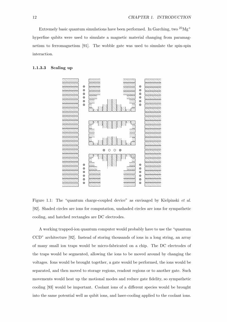
1.1.3.3 Scaling up
Figure 1.1: The “quantum charge-coupled device” as envisaged by Kielpinski et al.
[92]. Shaded circles are ions for computation, unshaded circles are ions for sympathetic
cooling, and hatched rectangles are DC electrodes.
A working trapped-ion quantum computer would probably have to use the “quantum
CCD” architecture [92]. Instead of storing thousands of ions in a long string, an array
of many small ion traps would be micro-fabricated on a chip. The DC electrodes of
the traps would be segmented, allowing the ions to be moved around by changing the
voltages. Ions would be brought together, a gate would be performed, the ions would be
separated, and then moved to storage regions, readout regions or to another gate. Such
movements would heat up the motional modes and reduce gate fidelity, so sympathetic
cooling [93] would be important. Coolant ions of a different species would be brought
into the same potential well as qubit ions, and laser-cooling applied to the coolant ions.
1.2. STRUCTURE OF THIS THESIS 13
The lasers would be far off-resonance from the qubits, and so would cause minimal
decoherence.
Many segmented traps have now been built and tested [94] (for instance, the NIST
error-correction and semiclassical QFT experiments were performed in one [61, 62]), and
some results have appeared for junctions [95, 96].
1.2 Structure of this Thesis
The general theme of this thesis is improving the fidelity of basic operations with trapped
ions. The problem is addressed directly, by simulating and implementing high-fidelity
readout and dynamical decoupling; and indirectly, by developing simulations and practi-
cal experience of the isotope 43Ca+. Until recently our group has worked with the most
common calcium isotope, 40Ca+, which has no hyperfine structure and so is simple to
work with. As mentioned above, 43Ca+ has hyperfine structure and so allows qubits with
long coherence times [58]. We thus expect to do many of our future experiments with
this isotope. So far our 43Ca+ work has been limited to coherence-time measurement
[58, 97] and sympathetic cooling [93].
Chapter 2 describes the apparatus that we have used – the trap itself, the control
system, lasers, signal generators and imaging system. I also present supplementary ex-
periments that measure the extinction provided by our optical switches, and observation
of unwanted polarisation variability in one of our beams.
Chapter 3 presents rate-equations simulations of 43Ca+. The background theory,
atomic data and computational details are presented, along with comparisons between
theory and experiment. I calculate certain off-resonant excitation processes that are
relevant to our experiments.
Chapter 4 describes high-fidelity readout of 43Ca+, with simulations and experi-
ments.
Chapter 5 describes an attempt to perform an entangling quantum gate between
one 40Ca+ ion and one 43Ca+ ion. This has potential value as part of a readout-free
quantum error-correction protocol. Unfortunately our attempt was unsuccessful, and
the rest of the chapter describes various noise problems with our apparatus.
Chapter 6 presents theoretical and experimental work on dynamical decoupling.
Dynamical decoupling is an extension of the basic spin-echo sequence that has recently

14 CHAPTER 1. INTRODUCTION
received much interest as a method of increasing the phase-coherence times of qubits.
Chapter 7 concludes and describes prospects for future work.

Chapter 2
Apparatus
Our experiments can be summarised as manipulating ions, and recording the results.
The ions themselves are singly-ionised calcium ions (Ca+, often written as Ca-II). They
are suspended by electric fields in ultra-high vacuum. Manipulations are performed with
up to ten lasers (and their attendant optics), microwaves and radio waves. Results are
recorded by collecting light from the ions with a series of lenses, and detecting the light
with a charge-coupled device (CCD) camera or photomultiplier tube (PMT). The lasers,
detection system etc. are all outside the stainless-steel vacuum chamber; the chamber
has windows and feedthroughs to allow light and electrical signals in and out. A personal
computer (augmented with specialist scientific electronics) controls the experiment and
saves the resulting data.
I shall start by introducing the calcium ion itself, and then go on to describe the ion
trap and the rest of the apparatus.
2.1 Calcium
2.1.1 Notation
P3/2, −1/2 specifies the (MJ = −1/2) Zeeman state of P3/2 in 40Ca+.
P4,+41/2 means the (F = 4, MF = +4) hyperfine state of P1/2 in 43Ca+.
P41/2 means the entire (F = 4) hyperfine manifold of P1/2 in 43Ca+.
P2;3;43/2 refers collectively to the (F = 2, F = 3, F = 4) hyperfine manifolds of P3/2 in
43Ca+.
I will refer to “levels”, by which I mean the fine-structure levels such as 4P1/2 and
3D5/2; “manifolds”, by which I mean the hyperfine-structure levels such as 4P41/2 or
15

16 CHAPTER 2. APPARATUS
3D15/2; and “states”, by which I mean states of specific magnetic quantum number such
as 4P4,+11/2 or 3D5/2, −3/2.
2.1.2 Levels and Transitions
4S1/2
3D5/2
t=1.168(7)s03
93
nm
Br=
93.4
7(3
)%
39
7n
mB
r=94
%
854n
m
Br=
5.87
(2)%
866n
m
Br=
6.0%
850n
m
Br=
0.66
1(4)
%
F=4
F=3
3226 MHz
3D3/2
t=1.176(11)s
4P3/2
t=6.924(19)ns
4P1/2
t=7.098(20)ns
MJ=-1/2
MJ=+1/22.8 MHz/G
43 +Ca
40 +Ca
Figure 2.1: The low lying energy levels of a Ca+ ion that are used in our experiments.
Lifetimes (τ) of the levels [14, 55, 98] and branching ratios (Br) of the transitions [20] are
labeled. 4S1/2 is labeled with the hyperfine splitting (for 43Ca+) or the Zeeman splitting
per gauss (for 40Ca+).
Figure 2.1 shows the energy levels and transitions of a calcium ion. They fall into
three broad groups depending on what we use them for:
S1/2 We use qubits which are stored in ground states of the ion. In 40Ca+, the two
Zeeman substates of S1/2 are the qubit states |↑〉 and |↓〉. In 43Ca+, the hyperfine
interaction splits S1/2 into two manifolds separated by 3.23 GHz. We can use any
of the pairs (S4,+41/2 ; S3,+3
1/2 ), (S4,-41/2 ; S3,-3
1/2 ) or (S4,01/2; S3,0
1/2) as a qubit. The latter choice
provides a “clock” qubit whose frequency is insensitive to the magnetic field to
first order, allowing quantum information to be stored for long periods with high

2.2. TRAPPING IONS 17
fidelity [58]; the other pairs are more prone to dephasing but are easier to prepare
in our experiment.
P1/2, D3/2, 397 nm, 866 nm The 397 nm transition is used in both isotopes for
Doppler cooling, qubit state preparation and fluorescence detection (see Chap-
ter 4). In 40Ca+, this transition is used for Raman transitions between the qubit
states to perform quantum logic gates and sub-Doppler cooling (see Section 5.1).
In 43Ca+, the Doppler cooling beam must have a 3.22 GHz sideband so that it
can excite from both hyperfine manifolds of S1/2 (see Section 3.4). The 866 nm
beam is required to repump from D3/2 – this level has a lifetime of 1.2 s, and P1/2
decays here once for every 15.7 scattered 397 nm photons (on average). The fluo-
rescence rate would be extremely low without effective repumping from this level
(see Section 3.4).
P3/2, D5/2, 393 nm, 850 nm, 854 nm These levels and transitions are used for read-
out: measuring which qubit state the ion is in. The general principle is to transfer
just one of the qubit states (say, |↑〉) to the long-lived D5/2 “shelf” level, and then
apply the Doppler beams – detecting fluorescence indicates that the ion was not
transferred to the shelf, and thus must have been in |↓〉. Chapter 4 describes the
process in more detail.
More details about the atomic structure constants of 43Ca+ can be found in Section
3.3, and Appendix A plots the hyperfine structure of its transitions.
2.2 Trapping Ions
The experiments described in this thesis were performed using a linear Paul trap. Paul
traps confine ions using an oscillating electric quadrupole1 field (usually at radio frequen-
cies, RF) – in the linear version, this field is produced by four long electrodes arranged in
a square (Figure 2.2). Each electrode is at the same RF phase as its diagonally opposite
partner; the pairs are in antiphase with each other. Averaged over a cycle of the field,
an ion feels a harmonic pseudopotential well centred on the null point of the field. The
RF null of a linear Paul trap is a line parallel to the electrodes – this defines the trap
axis z, and the RF confines the ion only in the perpendicular, radial directions.
1Higher-order multipoles can also be used as ion traps [99].
18 CHAPTER 2. APPARATUS
DC
DC
+RF
−RFz
1.01.21.6
1.3
4.2
1.22
Endcap
RF Electrode
DC Compensation
+RF
+RF
–RF
–RF
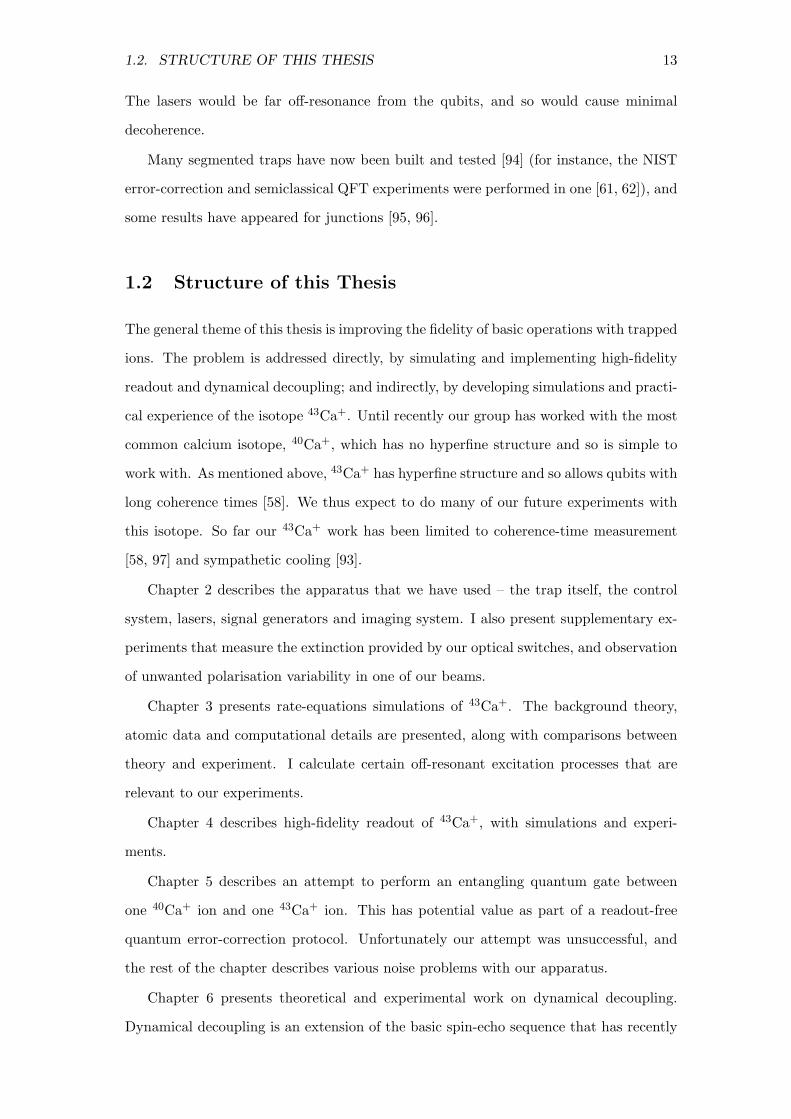
Figure 2.2: [Top] A perspective view of the RF and endcap electrodes. Ion pair not
to scale. [Bottom] Cross-sectional scale drawing of all the trap electrodes with their
dimensions in mm. Not shown, there are also 5.0 mm diameter support rods whose
centres lie on a square of side 18.4 mm. Also shown are the phases of the RF voltage.
Two endcap electrodes are placed at the ends of the trap, separated by 7.2 mm.
The endcaps are raised to a positive voltage (if, as in our case, the ion is positively
charged) producing a potential well that confines the ion in the z direction. The radial
(ωr) and axial (ωz) secular frequencies of the ion (i.e. the frequencies of the harmonic
pseudopotential wells) can be set separately within a wide range, although an ion of a
given charge:mass ratio will only be stably trapped for a certain range of voltages and
RF frequencies [100, 101].
Stray static electric fields are usually present and cause the equilibrium position of
the ion to be not quite at the RF null point. It hence feels an oscillating force from the RF
field, causing “micromotion” at the RF frequency that could be severely detrimental to
high fidelity quantum operations2. We balance out those stray fields using a further set
2In theory, because micromotion is coherent with the RF drive, the laser frequencies could be mod-
ulated to track the Doppler shift. Micromotion also manifests as sidebands on the laser transition and
a change in Rabi frequency, both of which can be measured and taken into account, or even be used
deliberately [102, 66]. But if more than one ion is trapped, micromotion can cause unwanted motional

2.2. TRAPPING IONS 19
of electrodes placed in a square outside, and parallel to, the RF electrodes. DC voltages
are applied to these to push the ion back into the RF null. In fact, we only need to
use the top two electrodes, the bottom pair being grounded (or used as a microwave
antenna, see Section 2.5.3). The procedure for setting the compensation voltages is
described in section 5.3.1.
The RF frequency is generated by a Colpitts oscillator with a fixed frequency of
6.4 MHz, with no further resonator or amplifier. It has two equal-amplitude outputs,
180 out-of-phase, that drive the two pairs of RF electrodes. This arrangement is atypi-
cal; linear Paul traps are often driven by oscillators with a single RF output, connected
to one diagonal pair of electrodes with the other pair grounded. Our oscillator’s am-
plitude can be varied manually (but not controlled by computer) up to ≈ 170 Vpk−pk.
The voltages on the endcaps and the top two compensation electrodes are independently
variable by computer up to ≈ 700 V, limited by breakdown of the vacuum feedthrough;
typical values 250-700 V for endcaps, < 100 V for compensation electrodes.
When various ion traps are compared [103, Figure 8 in preprint], the heating rate
of the ions is found to be approximately inversely proportional to the 4th power of the
trap size – usually defined as the smallest distance between an ion and any electrode
[104, 105]. In this trap the RF electrodes are closest to the ions, and the distance is
1.22 mm (Figure 2.2).
2.2.1 Tickling
The secular frequencies of an ion are most conveniently measured by “tickling”. We
apply an oscillating voltage to an endcap (to measure axial frequencies) or DC compen-
sation electrode (to measure radial frequencies), and scan its frequency while monitoring
the ion’s fluorescence. When the applied frequency is close to a motional frequency, the
ion will be driven into large oscillations that modify the ion’s fluorescence signal (or that
are visible with the camera). The quality factor of these oscillations is high (Q ∼ 2000)
so they can be measured precisely (to ± ∼ 0.2 kHz), but also care must be taken to avoid
driving the ion out of the trap. For the axial mode (the centre-of-mass mode, if there is
more than one ion), the resonance is just visible for tickle voltages ∼ 0.2 Vpk−pk; radial
modes are just visible at ∼ 1 Vpk−pk. Much larger amplitudes are used if the frequency
is unknown in advance, so that the resonance becomes visible in a coarse scan.
heating.
20 CHAPTER 2. APPARATUS
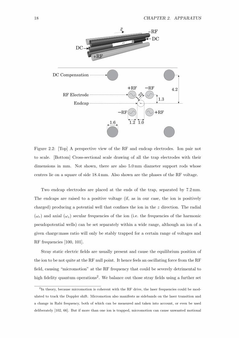
The radial pseudopotential is often assumed to be symmetrical, but we have been
able to measure two slightly different radial frequencies as shown in Figure 2.3. This
can happen due to accidental asymmetries in the construction of the trap, or stray
nonuniform DC electric fields. Non-degenerate radial frequencies are actually necessary:
if they were degenerate, then the principal axes of the radial modes can be in any
orientation. Applying a Doppler cooling laser beam can define these axes perpendicular
and parallel to the beam3. The ion can then remain hot in the direction perpendicular
to the beam. Ion trap designers often choose the radial modes to be non-degenerate,
and to have principal axes at 45 to the Doppler cooling beam. This forces the ion’s
radial vibrations to precess, and so both modes are cooled [12].
90 100 110 120 130 140 150 160 170300
400
500
600
700
800
900
1000
1100
Trap RF Voltage / Vpk−pk
Ra
dia
l S
ecu
lar
Fre
qu
en
cy /
kH
z
Lower mode: Data
Lower mode: Fit
Upper mode: Data
Upper mode: Fit
.
Figure 2.3: Radial secular frequencies of a single 40Ca+ as a function of trap RF ampli-
tude. Dotted lines indicate 50% confidence intervals of the linear fits. The micromotion
compensation was readjusted for every data point. The endcap voltages were constant
at 240 V and 238 V producing an axial frequency of 470 kHz for all the RF voltages.
3More precisely, parallel to the projection of the beam onto the trap’s x − y plane.

2.2. TRAPPING IONS 21
2.2.2 Loading
Near the trap is an oven, consisting of a thin-walled stainless-steel tube, loosely packed
with calcium granules and with a small hole in the side pointing towards the centre of
the trap. To load ions into the trap the tube is first heated by passing current (between
4 and 5 amps) through it; it heats up and sprays calcium atoms towards the trap. Two
lasers, at 423 nm and 389 nm, are used to ionise some of the atoms in a two-photon
process. The 423 nm beam (from a grating-stablised external-cavity diode laser) excites
the atoms on the 4s2 1S0 → 4s4p 1P1 transition. The natural width is 35 MHz, and
we take care to cross the atomic and laser beams at right angles to minimise Doppler
broadening: we observe the transition with a full-width half-maximum (FWHM) of
76 MHz. The smallest isotope shift of this transition (between Calcium-43 and Calcium-
44) is 160 MHz, so it is possible to excite predominantly one desired isotope. From
4s4p 1P1 an atom will be ionised by a photon of wavelength less than 389.8 nm; we
provide this light with an unstabilised 388.9 nm diode laser (with no external cavity).
If an atom is ionised near enough to the centre of the trap, and if correctly tuned
Doppler-cooling beams are applied, it will be caught.
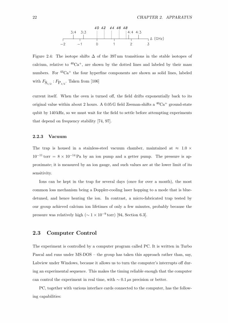
40Ca+, having 97% natural abundance, is relatively easy to load. 43Ca+ is much
more challenging because it makes up only 0.135% of natural calcium. We use much
higher intensity 389 nm light than for 40Ca+, and higher oven temperatures. We can
also ensure that only 43Ca+ ions are cooled by tuning the 397 nm Doppler laser just
red of the S41/2 → P4
1/2 hyperfine component of the transition, which is blue-detuned
from all other stable isotopes as shown in Figure 2.4 (the Doppler cooling laser must
have 3.22 GHz sidebands when working with 43Ca+; one sideband is red of all the other
isotopes in this situation, but its intensity is less than the carrier and so the net effect
is still to heat unwanted isotopes so they are not trapped). Full details of our loading
method can be found in Reference [106].
For the 40Ca+-43Ca+ experiments of Chapter 5, we would first load the 43Ca+. We
then retuned the ionisation and cooling lasers for 40Ca+, reducing the laser powers and
oven temperature so that the loading rate was ∼ 1 per minute, allowing us to load a
single ion.
While the oven is on, the magnetic field at the ion is altered (by ∼ 0.05 G), pre-
sumably because the hot metal becomes magnetised by ambient fields or by the oven
22 CHAPTER 2. APPARATUS
Figure 2.4: The isotope shifts ∆ of the 397 nm transitions in the stable isotopes of
calcium, relative to 40Ca+, are shown by the dotted lines and labeled by their mass
numbers. For 43Ca+ the four hyperfine components are shown as solid lines, labeled
with FS1/2: FP1/2
. Taken from [106]
current itself. When the oven is turned off, the field drifts exponentially back to its
original value within about 2 hours. A 0.05 G field Zeeman-shifts a 40Ca+ ground-state
qubit by 140 kHz, so we must wait for the field to settle before attempting experiments
that depend on frequency stability [74, 97].
2.2.3 Vacuum
The trap is housed in a stainless-steel vacuum chamber, maintained at ≈ 1.0 ×
10−11 torr = 8 × 10⁻¹⁴ Pa by an ion pump and a getter pump. The pressure is ap-
proximate; it is measured by an ion gauge, and such values are at the lower limit of its
sensitivity.
Ions can be kept in the trap for several days (once for over a month), the most
common loss mechanism being a Doppler-cooling laser hopping to a mode that is blue-
detuned, and hence heating the ion. In contrast, a micro-fabricated trap tested by
our group achieved calcium ion lifetimes of only a few minutes, probably because the
pressure was relatively high (∼ 1 × 10⁻⁹ torr) [94, Section 6.3].
2.3 Computer Control
The experiment is controlled by a computer program called PC. It is written in Turbo
Pascal and runs under MS-DOS – the group has taken this approach rather than, say,
Labview under Windows, because it allows us to turn the computer’s interrupts off dur-
ing an experimental sequence. This makes the timing reliable enough that the computer
can control the experiment in real time, with ∼ 0.1 µs precision or better.
PC, together with various interface cards connected to the computer, has the follow-
ing capabilities:
2.3. COMPUTER CONTROL 23
• It records photons that are detected by the PMT, counting how many fall within
definable-length time bins.
• It records analogue quantities such as photodiode measurements of laser powers.
• It sets and scans Digital-to-Analogue Converters (DACs) that control the trap DC
electrodes, laser frequencies, etc.
• It has “pseudo-DACs” for digitally controlling the frequencies and phases of our
high-precision synthesisers (for Raman or microwave transitions), using RS-232
serial ports.
• When necessary, it monitors the 50 Hz mains signal so that sequences can be
triggered at the same phase of the AC (to reduce magnetic field uncertainty, see
Section 6.4.1).
• When necessary, it monitors correlations between the trap RF and photon arrival
times, to allow micromotion compensation (see Section 5.3.1).
• It switches on/off laser beams via Acousto-Optic Modulators (AOMs) and shutters
(Section 2.4.5), and also microwaves and RF for magnetic resonance, in both cases
working through the Laser Control Unit described below.
• It switches on/off the oven, photoionisation beams and trap RF, for loading ions.
It has two main modes. The default is a continuous display of the PMT count
rate, photodiode readings and vacuum-system pressure. Lasers and other devices can
be switched and scanned manually. A “DAC scan” uses this mode while automatically
scanning a DAC over a pre-defined range, typically used to locate quickly the resonant
frequency for a laser.
In the second mode, the computer runs timed sequences. A “sequence” is a series
of instructions that mostly define laser or microwave/RF pulses, but can also change
DACs. A sequence typically initialises the ion(s) in the desired qubit state, performs
some quantum manipulations of the qubit(s), and finally performs a shelving read-out
(see Chapter 4) of the final qubit state(s). A sequence is repeated with identical settings,
usually between 200 and 1000 times, to obtain an estimate of the probability of the ion(s)
being shelved. This produces one data point. The computer changes something in the
sequence (either a DAC setting or a pulse time) according to the pre-defined scan range,

24 CHAPTER 2. APPARATUS
records the next point, and so on. The points collectively make up a “scan”. After
each sequence, the computer plots the number of photons counted and the photodiode
readings; this makes it easy for the experimenter to spot ion decrystallisations (see
Section 5.2.1) or laser frequency hops. In that case the scan can be paused while the
problem is fixed. At the end of the scan the data are saved.
A variant of the timed-sequence mode is “whizzo-interactive” mode. This allows
the sequence to be edited between each point, for optimising parameters or quickly
comparing different sequences.
2.3.1 Laser Control Unit
The Laser Control Unit (LCU) was designed and built by Ben Keitch [97]. It is the
interface between the computer and the physical devices, such as the switches that pass
or block the RF power to the AOMs. Most of the devices use standard 5 V TTL voltage
pulses, which the LCU supplies using buffer amplifiers to accommodate devices with
50 Ω input impedances. It provides accurate synchronisation of the pulses, with the
pulse times settable to 0.1 µs resolution. It also has a mechanical switch for each of the
16 channels, for convenient manual override.
2.4 Lasers
One of the advantages of using Ca+ is that we can use diode lasers to produce all
the necessary wavelengths, without frequency doubling. Short-wavelength laser diodes
(397 nm, 393 nm and 423 nm) have short lifetimes compared to those producing infra-
red (IR) light (in the ten years since the experiment was begun, we have had two of
our seven blue diodes fail, but none of the three IR diodes). They are not currently
manufactured, but when stocks run out it will be possible to produce those frequencies
by frequency-doubling light from IR laser diodes (indeed, this is necessary if beams of
more than ∼ 15 mW are required).
2.4.1 Summary of Lasers
Table 2.1 summarises our lasers. First I state whether the laser is a commercial Toptica
system or was built by the group, and whether it has a diffraction grating to provide
an extended laser cavity. Then I give the nominal maximum power output of the diode,
2.4. LASERS 25
after the grating if there is one (the output power of a diode is limited by its ability
to withstand the total optical power inside it, so if some light is reflected back into the
diode its own power output must be reduced). I briefly describe its uses, and state
what type of lock (if any) is used. Lasers are locked to temperature-stabilised, external
reference cavities, with ≤ 1 MHz/hr drift rates.
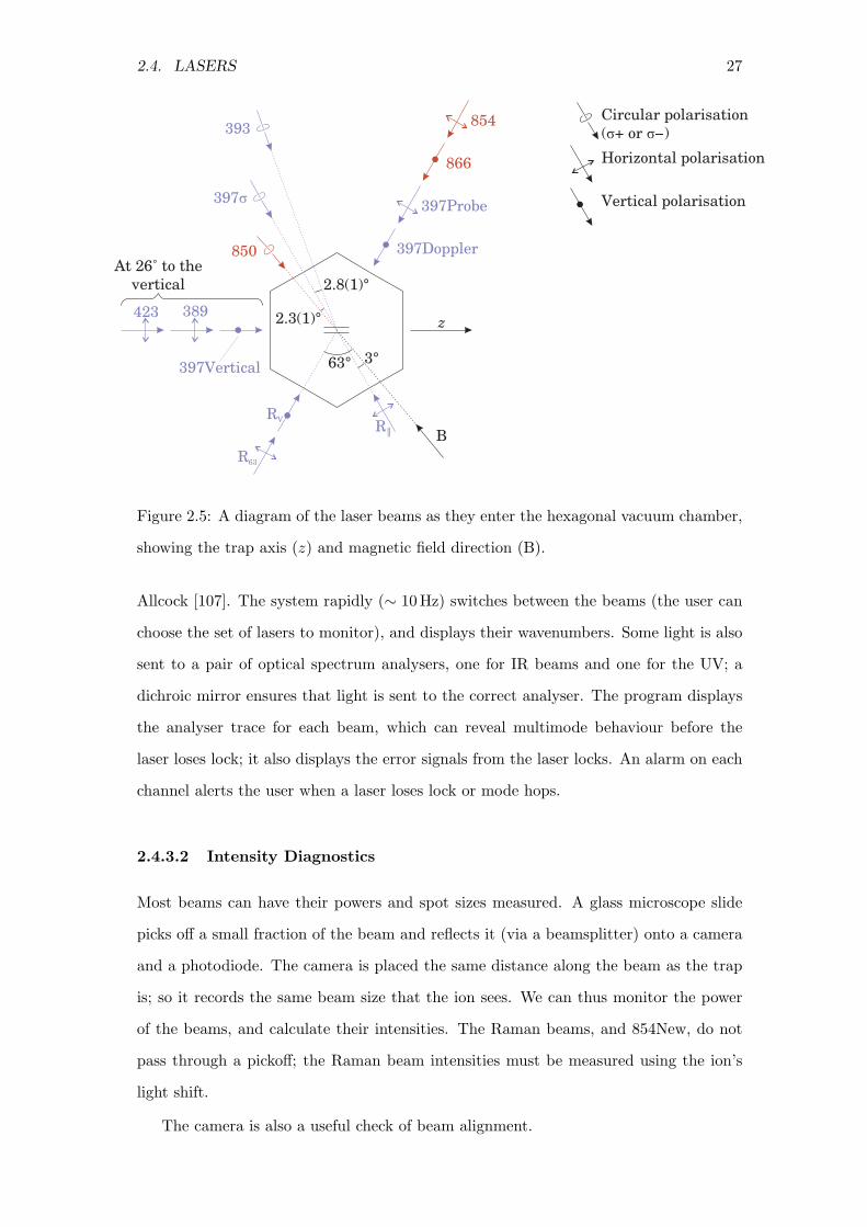
2.4.2 Beam Geometry and Polarisations
The geometry of the beams themselves, as they reach the ions, is shown in Figure
2.5. The four beams shown together in one line (397Doppler, 397Probe, 866 and 854)
are superposed using polarising beamsplitter (PBS) cubes and a dichroic mirror. R63
and RV are also superposed with a PBS cube; so is 397Vertical combined with the
photionisation beams (which come from the same optical fibre). Each of the circularly
polarised beams has a λ/4 waveplate to allow them to drive σ+ or σ− transitions, or
can be made linearly polarised to drive both.
The magnetic field B is shown as it would be set for experiments with 40Ca+ –
carefully aligned with the 850 nm beam for high σ polarisation purity at the ion, which
is needed for the EIT readout process in that isotope (summarised at the start of Chapter
4). Readout of 43Ca+ is actually improved if the 850 nm beam is slightly off the magnetic
field direction (Chapter 4), and so for experiments with this isotope we align B with the
397σ state-preparation beam.
The vertical beams (423, 389 and 397Vertical, which is only used to detect vertical
micromotion) enter the chamber through the same window that the imaging system looks
through. A small black-paper flag is placed just below the imaging system’s objective
lens, to prevent reflections of these beams entering the imaging system.
2.4.3 Diagnostics
2.4.3.1 Frequency Diagnostics
Every laser has a little light (20 µW to 2000 µW) split off from the beam into its own
multimode optical fibre (except the 389, which is not monitored because its frequency
is unimportant; the 423 and 850 lasers share a fibre with one beam blocked at any
time). The fibres are connected to a HighFinesse WS/7 wavemeter via an eight-channel
fibre switcher, both under the control of a Labview computer program written by David

26C
HA
PT
ER
2.
AP
PA
RA
TU
S
Name, Approx Max
Wavelength / nm Model Grating? Power / mW Uses and Notes Lock (see Section 2.4.4)
423 Toptica DL100 Yes 15 Isotope-selective excitation for photionisation. None
389 Home-made No 2 Non-selective second stage of photoionisation. None
397D40 Toptica DL100 Yes 15 Provides beams for Doppler cooling, state preparation and contin-
uous Raman cooling of 40Ca+ (which uses the beams 397σ and
397Probe).
PDH lock via EOM
397D43 Toptica DL100 Yes 15 Provides beams for Doppler cooling and state preparation of 43Ca+. PDH lock via current modula-
tion, with fast current feedback
866 Home-made Yes 50 Repumps from D3/2. Side-of-fringe lock
397 Master/Slave Toptica DL100 Yes 30 Produces the beams R‖, R63 and RV, used for Raman transitions in
40Ca+ (Rabi flopping, pulsed sideband cooling) and for the travelling
standing wave of Chapter 5. See Section 2.4.6.2 for details.
None
393 Toptica DL100 Yes 5 Shelves ions during readout. PDH lock via EOM
854Old Home-made Yes 25 Deshelves the ions, returning them to the ground level from D5/2
after readout is complete. The grating of this laser was replaced due
to falling power output, but has performed extremely poorly (it can
only be tuned a small amount before modehopping).
None
854New Toptica DL100 Yes 45 Temporary replacement for 854Old. This beam is delivered by optical
fibre from the laboratory next-door.
None
850 Home-made Yes 100 Used for readout. For 40Ca+, it creates a dark resonance so only one
of the qubit states is shelved. For 43Ca+, it repumps the ion if it falls
into D3/2 rather than D5/2. See Chapter 4 and Section 2.7.2.
Side-of-fringe lock
Table 2.1: Summary of the lasers used in the experiment.
2.4. LASERS 27
z
397Doppler
397Probe
866
854
R
R63
RV
B
850
397σ
393
2.8(1)°
2.3(1)°
63° 3°
Circular polarisation
( + or −)σ σ
Horizontal polarisation
Vertical polarisation
397Vertical
423 389
At 26˚ to the
vertical
Figure 2.5: A diagram of the laser beams as they enter the hexagonal vacuum chamber,
showing the trap axis (z) and magnetic field direction (B).
Allcock [107]. The system rapidly (∼ 10 Hz) switches between the beams (the user can
choose the set of lasers to monitor), and displays their wavenumbers. Some light is also
sent to a pair of optical spectrum analysers, one for IR beams and one for the UV; a
dichroic mirror ensures that light is sent to the correct analyser. The program displays
the analyser trace for each beam, which can reveal multimode behaviour before the
laser loses lock; it also displays the error signals from the laser locks. An alarm on each
channel alerts the user when a laser loses lock or mode hops.
2.4.3.2 Intensity Diagnostics
Most beams can have their powers and spot sizes measured. A glass microscope slide
picks off a small fraction of the beam and reflects it (via a beamsplitter) onto a camera
and a photodiode. The camera is placed the same distance along the beam as the trap
is; so it records the same beam size that the ion sees. We can thus monitor the power
of the beams, and calculate their intensities. The Raman beams, and 854New, do not
pass through a pickoff; the Raman beam intensities must be measured using the ion’s
light shift.
The camera is also a useful check of beam alignment.
28 CHAPTER 2. APPARATUS
2.4.4 Locking
We need many of our lasers to have better frequency stability than they achieve pas-
sively. In all these cases we lock each laser to its own Low-Drift Etalon (made by the
National Physical Laboratory, NPL). The mirrors in these cavities have “W” reflective
coatings – achieving high reflectivity for both our IR and UV wavelengths (giving fi-
nesses of ≈ 30 − 520, depending on the required linewidth). Their free spectral range
(the frequency separation of cavity resonances) is 1.5 GHz.
For a side-of-fringe lock, the transmitted power through the cavity is monitored.
That power has a narrow peak when the beam is resonant with the cavity. Feedback
electronics are engaged to keep the laser at the frequency corresponding to about half-
way up this peak – the point of maximum gradient providing narrowest laser linewidth.
A Pound-Drever-Hall (PDH) lock [97, 108] is more complicated but more robust than
side-of-fringe. It is not affected by a change in the power of the laser, as side-of-fringe
locks are vulnerable to. A PDH lock has a higher “capture range” of frequencies, so that
a laser that makes a sudden jump (up to ∼ 100 MHz) will be brought back to its set
point rather than break out of lock. Sidebands are put on the beam by modulating the
laser current, or by using an Electro Optic Modulator (EOM), and the locking signal is
reflected from the cavity.
In both cases, the locking electronics feed back and adjust the frequency of the laser.
All the locked lasers are grating stabilised, in the Littrow configuration. The beam
straight out of the diode hits a diffraction grating at an angle chosen to be the first
order diffraction angle for the desired wavelength. The first order diffracted beam is
thus reflected back into the diode, the grating acting as one mirror of the laser cavity.
The zeroth order is the laser’s output beam. Coarse frequency tuning is by rotating
the grating in the horizontal direction. Fine frequency tuning is by translating the
grating towards (away from) the laser to shorten (lengthen) the laser cavity and shorten
(lengthen) the wavelength. A piezo-electric actuator can perform this fine tuning, and
this is one way in which the lock controls the laser frequency. It also adjusts the current
supply to the laser diode, providing faster feedback (and hence narrower linewidth) as
well as reducing the probability that the laser hops to a different mode.
The 397D43 has an extra current feedback path to a field effect transistor (FET)
that can alter the diode supply current extremely fast (5 MHz bandwidth). This greatly

2.4. LASERS 29
reduces the laser jitter as deduced from the PDH error signal – from ±10 MHz to
±0.4 MHz. Testing using ion fluorescence, however, was unable to detect any differ-
ence in linewidth from using the FET feedback, and suggested that the linewidth was
always . 5 MHz.
The reference etalons have one mirror which can be translated with piezos. We can
thus change the resonant frequency of the cavity, and hence scan the laser: provided
it is scanned slowly compared with the lock bandwidth, the locked laser will follow the
cavity.
2.4.5 Switching and Fine Frequency Control
Beams are switched on and off by Acousto-Optic Modulators (AOMs). These are made
from crystals whose refractive index changes signifcantly when the material is com-
pressed. An acoustic wave (typically 80 MHz or 200 MHz) is passed through the crystal
(as a travelling wave, rather than a standing wave) to create a travelling diffraction
grating. When the wave is being driven, the ±1st-order diffracted beams are Doppler
shifted by ± the drive frequency. The input beam is carefully aligned to maximise the
strength of the chosen diffracted beam, and that beam then continues to the ion. The
zeroth order (and any others that may be present) is usually blocked; but sometimes
the zeroth order continues to the input of the next AOM (such as the 397 nm σ and
Doppler AOMs) or a diagnostic (854Old).
Even when an AOM is nominally switched off, the diffracted beam is not perfectly
extinguished. Two possible reasons include imperfect extinction of the RF drive, and
scattering from the AOM crystal. The former is believed to be dominant. Section 2.7
describes some experiments that investigated AOM extinction.
For the Raman beams (R‖, R63 and RV), and 397Probe, the switching AOMs are
also used to control the frequency. This is because the relative frequencies of the Raman
beams must be variable, as well as the frequency difference between 397Probe and
397σ (which are used for continuous Raman cooling of 40Ca+, but will not be called
“Raman beams” in this thesis). Usually, changing the frequency of an AOM causes
the deflection angle to change; we prevent this by placing a lens after each of these
AOMs (imaging the middle of the AOM onto the ion). The 397Probe AOM is powered
by a commercial IntraAction DE series AOM driver; this has a frequency modulation
input that is driven by a DAC from PC. The Raman beams are driven by versatile,

30 CHAPTER 2. APPARATUS
high-precision synthesisers via amplifiers.
2.4.6 Laser-Specific Details
2.4.6.1 397D40 and 397D43
The lasers 397D43 and 397D40 can be used to produce four different beams: 397Doppler,
397σ, 397Probe and 397Vertical. Their optics is therefore more complex than the other
beams (Figure 2.6), and so will be explained here.
“Master” AOM
(double-pass)
EOM
3.22 GHz
σ AOM
200 MHz
Doppler AOM
80 MHz
Probe AOM
200 MHz
λ
2
397D43
Laser
397D40
Laser
To wavemeter, optical spectrum
analyser and PDH lock.
Diffraction
grating
Diffraction
grating
Shutter
To wavemeter, optical spectrum
analyser and PDH lock.
50% beamsplitter
non-polarising
PBS
397
beam
σ
397Vertical
beam
397Doppler
and 397Probe
beams
Figure 2.6: A highly schematic diagram showing the 397 nm beams.
Both lasers, as well as having a diffraction grating as part of their laser cavity, have
a second grating to reduce the amount of amplified spontaneous emission (ASE) that
reaches the ion (otherwise these lasers would produce enough light at 393 nm to shelve
the ion ∼ once per second [100]). Additionally, for 397D43 this grating splits off beams
for the PDH lock and the frequency diagnostics. The beam from 397D40 passes twice
through a “Master” AOM to improve the extinction (to better than 1 : 30 000 = −45 dB
[109, Table 3.3]); however each pass only deflects ≈ 60% of the power. The beam
from 397D43 is switched using a mechanical shutter that gives perfect transmission and
extinction; however it requires careful timing when used in a timed sequence experiment
(see Section 2.7.1.2).
The beams then meet at a 50% beamsplitter cube. One output leads to the 397σ and

2.4. LASERS 31
397Doppler AOMs, the zeroth order of the former is the input to the latter because we
almost never need to use those beams at the same time. The other beamsplitter output
leads to the 397Probe AOM. The probe and Doppler beams are combined at a PBS
cube. The probe beam is transmitted because it is horizontally polarised. The Doppler
beam can be reflected or transmitted to any desired degree using the λ/2 waveplate,
allowing the use of the vertical beam when it is needed for micromotion compensation.
2.4.6.2 397 Master/Slave
The Master is a grating-stabilised 15 mW laser whose light is injected into the front
of the Slave diode. The Slave has no grating, but coherently amplifies the light from
the Master. The pair combines the low linewidth of grating-stabilisation with the high
power possible from a diode with no external cavity.
The individual beams it produces (R‖, R63 and RV) are each switched with single-
pass AOMs.
2.4.6.3 393
The 393 nm laser is switched by a double-pass AOM. There is a 1938 MHz EOM for
simultaneous shelving of 43Ca+ and 40Ca+ (see Section 5.1.2).
2.4.6.4 866
The 866 nm laser is switched by a double-pass AOM, and has a second diffraction grating
to greatly reduce the effect of ASE [55].
The 866 nm transitions of 40Ca+ and 43Ca+ are separated by an isotope shift of
3464 MHz, which is close to the S1/2 hyperfine shift of 43Ca+ (3226 MHz). This allows
us to drive a second EOM from the 3220 MHz oscillator that powers the 397D43 EOM;
and since the 866 nm transition of 43Ca+ is spread over 770 MHz of hyperfine shift, we
can obtain a reasonable fluorescence rate from both isotopes without retuning the laser.
This is vital for doing readout from both ions during a 40-43 experiment.
2.4.6.5 854Old and 854New
854Old is switched by a single-pass AOM. For sensitive experiments (such as the readout
experiments of Chapter 4) a shutter can be used as well. 854New is switched by a double-
pass AOM.
32 CHAPTER 2. APPARATUS
2.4.6.6 850
The 850 nm laser is switched by a single-pass AOM. The laser and AOM are on a different
optical table to the vacuum system, with the light being transferred by a polarisation-
maintaining optical fibre. In Section 2.7.1.1 I describe a measurement of the extinction
produced by the AOM when the beam is switched off, and Section 2.7.2 describes how the
optical fibre produces periodic changes in the polarisation of the beam (which translates
to power variability at the ion, because PBS cubes are used to polarise the beam after
the fibre).
2.5 Coherent Manipulation
There are three main methods we can use to perform coherent single qubit operations.
These are the Raman beams (in 40Ca+), magnetic resonance at ∼ 5 MHz (in 40Ca+)
and microwaves at ∼ 3.2 GHz (in 43Ca+).
We directly apply qubit rotations only if their axes are perpendicular to the z axis –
including σx and σy Pauli operators, for instance, but not phase shifts about the z axis.
Instead of applying a phase gate, we change the phase of the radiation that drives the
coherent manipulations. The x and y axes are essentially arbitrary, being fixed by the
phase of the first coherent pulse applied to the ion.
2.5.1 Magnetic Resonance
For us, “magnetic resonance” refers to driving the S1/2, +1/2 ↔ S1/2, −1/2 magnetic
dipole transition in 40Ca+ with an oscillating magnetic field. The Zeeman splitting
is 2.8 MHz/ G, which gives 4.8 MHz at 1.7 G. The field is produced by amplifying a syn-
thesizer output with a Frankonia FLL 25 amplifier, emitting up to 25 W = 44 dBm. The
amplifier output drives a 40-turn coil which is mounted just outside the large imaging
window of the vacuum chamber. The coil has two layers of 20 turns each, sits around
the imaging system tube and is conical in shape to allow the vertical laser beams to
pass outside it. Its resonance can be tuned from 4.1 MHz to 4.9 MHz using a variable
capacitor in series with the coil; the resonance width is ∼ 250 kHz [110]. The amplifier
is particularly robust and is not affected if the RF load is a short- or open-circuit, so we
do not impedance-match the coil to 50 Ω.
In practice the maximum power is limited by breakdown of the (air-spaced) variable

2.5. COHERENT MANIPULATION 33
capacitor, and because other pieces of equipment in the laboratory (such as laser locks)
start to pick up the radio signal at high powers. The highest Rabi frequency is ≈ 5 kHz
(π-time of 100 µs). Such slow Rabi-flopping means that single-qubit gates are highly
susceptible to magnetic field drift.
2.5.2 Raman Transitions
We achieve faster Rabi flops by driving Raman transitions between the Zeeman states.
Raman transitions use two far-detuned 397 nm laser beams, whose frequency difference
equals the Zeeman splitting. It is vital that the beams are coherent with each other, so
we derive them both from the 397 Master/Slave laser. In this case the beams do not
excite the ion to P1/2; instead, by a process called adiabatic elimination, coherent Rabi
oscillations are driven between the two ground states [74].
The 397 Master/Slave laser is typically set to a wavenumber ≈ 25190.3 cm−1, a
detuning of ≈ 40 GHz below the 397 nm resonance. The beams R63, RV and R‖ usually
have powers from 100 µW to 600 µW each, depending on the desired Rabi frequency for
the current experiment.
We used to use R63 and R‖ for Raman transitions. The difference wavevector of
these beams lies along the trap z axis – deliberately, so that they can be used for Raman
cooling. But this coupling with the ions’ motion means that at high temperatures, the
fidelity of Rabi oscillations is reduced (even if the difference frequency is tuned to the
carrier transition rather than a motional sideband).
For the work of Chapter 5 we changed to using the beams R63 and RV. They co-
propagate so we can drive qubit transitions without affecting or being affected by the
ion’s motion. Beam powers of 540 µW gave a Rabi frequency of 200 kHz (a π-time of
2.6 µs).
2.5.3 Microwave Transitions
In 43Ca+, the magnetic dipole transition between the qubit states (the hyperfine levels
of S1/2) are approximately 3.2 GHz, in the microwave region of the spectrum. Dr. Keitch
[97] studied the best way of driving these transitions. He tested four types of antennae
mounted outside the vacuum chamber, including a magnetic loop, a λ/2 dipole and a
cylindrical horn antenna. The horn was the best of these, and was successfully used
to detect the resonance of an ion. However, superior results were obtained when the

34 CHAPTER 2. APPARATUS
microwave signal was applied to one of the trap’s DC compensation electrodes (in the
vacuum chamber, of course) – the Rabi frequency increased by a factor of ∼ 100 due to
more efficient coupling from the antenna to the ion.
No effort was made to match impedance between the antenna and the 50 Ω output
of the amplifier. The power reflected to the amplifier is 7 dB (a factor of 5) lower than
the power emitted, and it is not known how much of this reflection is from the electrode
itself and how much is from the vacuum feedthrough. The amplifier is a Minicircuits
ZVE-8G that puts out nearly 29 dBm ≈ 750 mW, and we can drive Rabi oscillations at
up to 18 kHz (π-time of 30 µs).
2.5.4 Synthesiser Network
In Figure 2.7 I show the arrangement of switches and synthesisers that control the
coherent qubit operations. For the operations that demand the greatest flexibility and
frequency stability from their signal generators, we use Agilent ESG synthesisers. These
are either from the ESG-A series (E4422B) or the ESG-AP series (E4426B), the major
difference being that the APs have higher spectral purity. They all operate from 250 kHz
to 4 GHz, and have a wide range of control options. In particular, we use three methods
of controlling their output – manual (the front panel); digital, (RS-232 interface via the
serial/COM port on PC); and analogue (TTL on/off as well as modulation of amplitude,
phase, frequency, etc.). We use the digital interface to precisely set the synthesiser’s
frequency or phase from PC, but this is too slow to use within a timed-sequence and so
is limited to being changed between data points. Analogue control is fast enough to use
within a sequence (typical modulation bandwidths up to 1 MHz), for instance to change
the phase between the two π2 -pulses of a Ramsey experiment.
We ensure long-term stability by using a rubidium frequency reference (Stanford
Instruments FS725), whose frequency has an Allan variance of < 2×10⁻¹² over 100 s. It
produces a 10 MHz output that is used as the master clock by all our Agilent synthesizers.
Certain operations do not need such high specification synthesisers. Specifically,
when we perform pulsed Raman sideband cooling we drive one of the Raman beams with
Marconi 2019A signal generators. We set them manually to the desired frequency for a
stretch or centre-of-mass red sideband pulse, and do not need modulation or computer
control.

2.5. COHERENT MANIPULATION 35
Synth 1
ESG-A
VCO
VCO
Synth 5
ESG-AP
Synth 4
Marconi
Synth 3
Marconi
[Unused]
Synth 6
ESG-AP
Synth 2
ESG-A
Y(Two switches
controlled together)
X
PM
ΦM
COM
PM
ΦM
COM
00
0
0
1
1
1
1 0
1
0
1
0
1
0
1
1W R AOM63
R AOMV
R AOM
Microwave antenna(BR compensation electrode)
397D43 EOM
866 EOM
393 EOM
50:50 power
splitter
1W
200
200+fZ
200+ ±fZ δ
200+ − −f fZ Str Wδ
200+ −f fZ Str
200+ −f fZ CoM
1938
3220
fHf ±δ
Frequency
/ MHz
Synthesizerwith modulations
used
TTL SwitchesAmplifer
with max. power
or
1W
1W
1W
4W
4W
Figure 2.7: The network of synthesizers and switches as used for the experiments of
Chapter 5. fZ ≈ 4.7 MHz is the Zeeman splitting of the 40Ca+ qubit states; fHf ≈
3.2 GHz is the splitting of the 43Ca+ qubit states; fStr and fCoM are the frequencies of
the stretch and centre-of-mass motional modes; δW is the detuning of the “wobble” gate
pulse; and δ represents the detuning that may be applied during a scan over a Raman
or microwave resonance. The possible modulations are: pulse modulation (PM), a TTL
switch internal to the synthesizer; analogue phase modulation (ΦM); and digital control
of phase and frequency by RS-232 (COM).

36 CHAPTER 2. APPARATUS
2.6 Imaging System
We have two reasons for observing the ions. We must be able to count how many ions
are in the trap (and whether they are the desired isotope), and we must be able to
measure the state of the ion(s). We typically use different instruments for each purpose
– a camera is used to image the centre of the trap, allowing us to easily see individual
fluorescing ions; and a PMT counts UV photons scattered by the ions, allowing high
fidelity readout (as in Chapter 4, and in Myerson et al. [82]). Both devices receive light
from the ions via the same imaging system. In normal operation, light is collected by
a large aperture objective lens and travels up the imaging system’s light-tight tube to
the PMT. There is a pinhole just in front of the PMT to reduce background counts –
the lens(es) focuses an image of the ions onto this pinhole for maximum transmission.
A beamsplitter (power transmission 18% at 397 nm) can be rotated into place to reflect
most of the light to the camera, with the ions being imaged on the camera’s CCD.
Originally the objective focused the ions’ image several centimetres below the beam-
splitter. Here there was a movable aperture (700 µm× 870 µm[100]) and a shutter. The
shutter could be closed to protect the camera and PMT from bright light in the days
of electron-bombardment ionisation; it is obsolete now photoionisation is used. Then
there were three additional lenses before the beamsplitter, camera and PMT, which fo-
cused the light onto the instruments. Coloured-glass blue band-pass filters were used to
further reduce background light. Donald [100] calculated the collection efficiency to be
0.13(2)%, and measured it (by comparing the maximum count rate from a fluorescing
40Ca+ with a 3-level system rate-equations model) to be 0.11%, a figure confirmed by
later work.
The imaging system was significantly simplified partway through this work (2nd
April 2008) to improve the collection efficiency – each lens and filter absorbed or reflected
some of the ion fluorescence we try to observe, so removing them would increase the
photon count rate and make readout faster and more accurate. The movable aperture
and shutter were also removed. Both versions used the same objective lens (Nikon
ED PLAN 1.5x SM2-U, a compound lens with ≈ 70 mm focal length (although the
nominal value is 65 mm [100]). The system now contains only one lens (the objective),
no wavelength filters and just one spatial filter (the PMT pinhole).

2.6. IMAGING SYSTEM 37
Also, the objective lens was moved downwards by 4 mm4, which both increases the
light collection angle (and hence the collection efficiency, by ≈ 13%) and moves the
ions’ primary image upwards. The geometrical collection efficiency ǫg of the objective
is, according to the lens specifications, given by the radius ra = 17 mm of its effective
aperture and the distance from the bottom of the lens cowling to the ion rd = 66(2) mm.
Then we have
ǫg =πr2
a
4πr2d
= 0.0167(20) (2.1)
which is indistinguishable from the value in [100]. I have estimated the uncertainty as
being the difference between the equivalently-calculated value in Ref. [100] (0.016) and
a value measured in that work by using a known, variable aperture (0.018(2)).It is now
the primary image that is focused onto the camera CCD and PMT pinhole.
Figures 2.8 and 2.9 respectively show the old and new imaging systems.
I measured the transmission, at 397 nm, of the lenses and glass filters removed from
the imaging system. A power meter was used to measure the power of a beam before
and after an element, or set of elements. When using the lenses, care was taken that the
transmitted spot was placed in the same position, with approximately the same size, as
the laser spot measured before the lens. Results are shown in table 2.6. Combinations
Optical element (refer to Figure 2.8) Power transmission at 397 nm
Filter BG38 77.2(3)%
Filter BG37 83(2)%
Lens 50PS25 87.5(3)%
Lens 50DQ16 86.6(3)%
Lens 100DQ25 65.8(3)%
of the optical elements were also measured, suggesting that the filter and two lenses
in the PMT (camera) light path transmitted only 63(1)% (45(1)%) of the light from a
fluorescing ion. Previously the lenses’ transmission had been measured as 92% each at
397 nm [100].
We can estimate the total efficiency of the new imaging system by multiplying to-
gether:
4The lens was moved down by 4 mm relative to its position just before the rebuilding; but it is only
≈ 1 mm lower than shown in [100] and Figure 2.8.
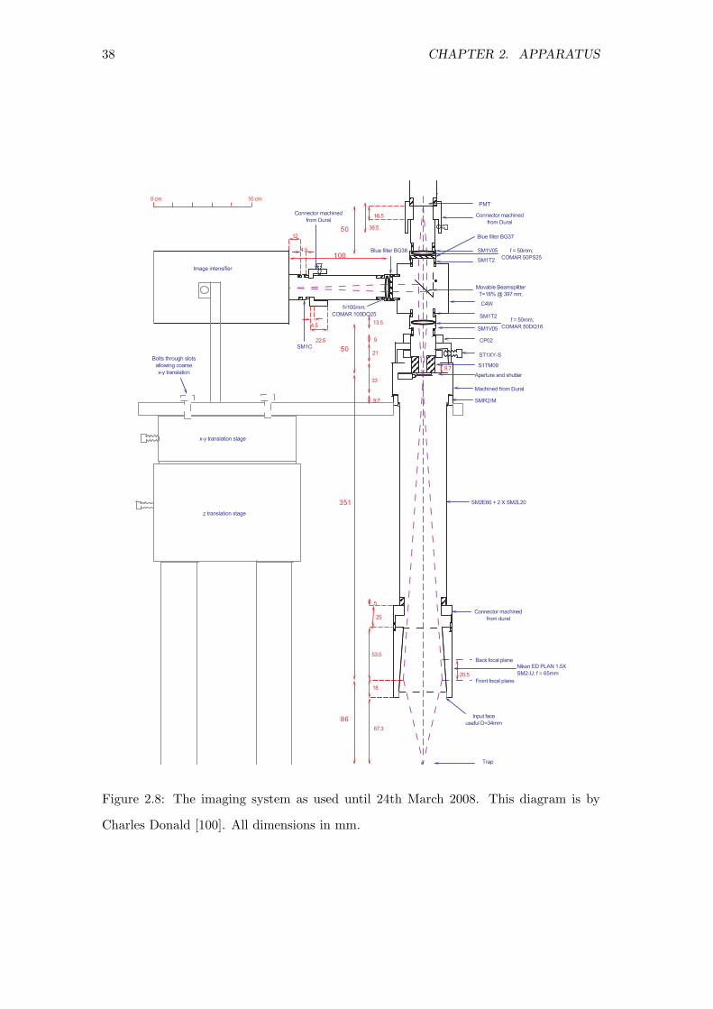
38 CHAPTER 2. APPARATUS
Figure 2.8: The imaging system as used until 24th March 2008. This diagram is by
Charles Donald [100]. All dimensions in mm.

2.6. IMAGING SYSTEM 39
Taken or deduced from CJD’s thesis, Fig 3.30Measured by DJS from actual system.
24
51
134
55.8
18
328
11
51
22.54.5
16.536.5
2520.5
5571.5
18
PMT
Connector(Machined from Dural)
C4W (Machined to make room forBeamsplitter, not shown)
Movable BeamsplitterT = 18% @ 397nm(Pivot not correctly positionedon diagram; illustration only)
SM2L20
SM2L20
SM2E60
SM1L20
SM1NT
2 x SM1NT
Mounting Plate(Machined from Dural)
Connector(Machined from Dural)
Nikon ED PLAN 1.5xSM2-U; f = 65mm (Nominal)( )Front and Back focal planes
Ion
Vacuum System Window(Top Surface)
Input Face(Useful D = 34mm)
Connector(Machined from Dural)
Andor CCD Camera(DU437-BU2)
X-Y Translation Stage
Z Translation Stage Inside coated withblack card toreduce reflection
Circle of black cardto reduce reflection
Pinhole
Bolts through slots allowcoarse X-Y translation
Figure 2.9: The imaging system as used after 2nd April 2008. All dimensions in mm.
Dimensions taken from or deduced from Donald [100] are shown in orange and sans-serif
font; those in serif font and dark red were measured by the current author.
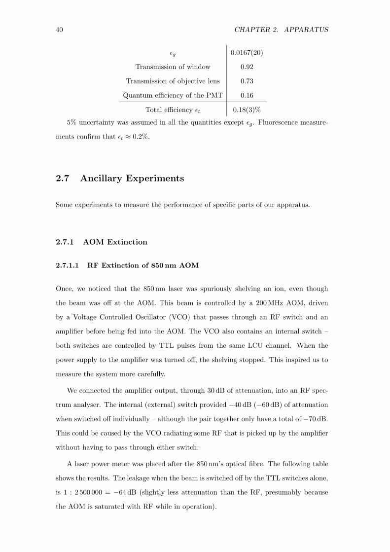
40 CHAPTER 2. APPARATUS
ǫg 0.0167(20)
Transmission of window 0.92
Transmission of objective lens 0.73
Quantum efficiency of the PMT 0.16
Total efficiency ǫt 0.18(3)%
5% uncertainty was assumed in all the quantities except ǫg. Fluorescence measure-
ments confirm that ǫt ≈ 0.2%.
2.7 Ancillary Experiments
Some experiments to measure the performance of specific parts of our apparatus.
2.7.1 AOM Extinction
2.7.1.1 RF Extinction of 850 nm AOM
Once, we noticed that the 850 nm laser was spuriously shelving an ion, even though
the beam was off at the AOM. This beam is controlled by a 200 MHz AOM, driven
by a Voltage Controlled Oscillator (VCO) that passes through an RF switch and an
amplifier before being fed into the AOM. The VCO also contains an internal switch –
both switches are controlled by TTL pulses from the same LCU channel. When the
power supply to the amplifier was turned off, the shelving stopped. This inspired us to
measure the system more carefully.
We connected the amplifier output, through 30 dB of attenuation, into an RF spec-
trum analyser. The internal (external) switch provided −40 dB (−60 dB) of attenuation
when switched off individually – although the pair together only have a total of −70 dB.
This could be caused by the VCO radiating some RF that is picked up by the amplifier
without having to pass through either switch.
A laser power meter was placed after the 850 nm’s optical fibre. The following table
shows the results. The leakage when the beam is switched off by the TTL switches alone,
is 1 : 2 500 000 = −64 dB (slightly less attenuation than the RF, presumably because
the AOM is saturated with RF while in operation).

2.7. ANCILLARY EXPERIMENTS 41
VCO Amplifier Switches Blocked
power power TTL with card Power
on on on no 3.62 mW
on on off no 1.5 nW
off off off no ≈ 0.8 nW
off off off yes ∼ 0.1 nW
The 1.5 nW could have been the cause of the shelving. However, the problem did
not recur so we did not attempt to improve the extinction.
2.7.1.2 Extinction of 397 nm beams
The beams produced by the 397D40 laser have two stages of extinction: the beam goes
through a double-pass “Master” AOM, then is split into the Doppler, σ and probe
beams each of which has its own, independently switched, single pass AOM. A double-
pass AOM is not expected to be as effective at blocking a beam as two separate AOMs,
because of RF leakage effects as described in the previous section. However, this ar-
rangement reduces leakage of resonant 397 nm light enough to allow coherence times up
to ∼ 1 s [97].
The 397D43 laser does not have a “Master” AOM – only the individual AOMs in
the three product beams. So to prevent leakage, a mechanical shutter is placed in the
beam path. This provides near-total extinction of the beam. However, the experimental
sequence must be carefully timed around it because it is prone to bouncing (blocking
the beam when it should be open, or vice-versa) and has a variable delay 1-4 ms between
receiving the open/close signal and acting.
For some of the readout experiments (see Section 4.3) a similar shutter was used in
the 854 nm beam. Figure 2.10 shows the control TTL signal sent to this shutter, and
the power of the beam as measured by a pick-off photodiode. Notice the wide time
variability of the shutter. The 397D43 shutter is similarly variable.
This variability makes shutters awkward to use in sequences. If long coherence
times are required (such as in the two-qubit gate experiments of Chapter 5, or the dy-
namic decoupling experiments of Chapter 6) then the shutter is essential to perfectly
block the beam between the state-preparation and fluorescence-detection stages of the
sequence. Otherwise photons can leak through an AOM and change the state of the
ion. But shorter experiments, or those that don’t need very high fidelity, can be con-

42 CHAPTER 2. APPARATUS
Figure 2.10: Screenshot from a mixed-channel oscilloscope that shows the pulse sequence
and beam powers as measured by pickoff photodiodes. The upper red line is the control
TTL signal “∼854S” sent to the 854 nm shutter (logic low means “open”). The lower
red region shows the 854 nm beam power (down means higher power). For the power
measurement, the scope was set to “persist” so that previous traces stayed on the screen
– that gives the lighter red area, while the darker line is the instantaneous reading. Note
where the shutter has previously bounced partially closed (circled in red). For scale, the
green vertical dashed lines are separated by 20 ms, the repetition period of the sequence.
veniently performed without the shutter. Unlike the 854 nm and 850 nm beams, the
397 nm Doppler AOM (and all the other 397 nm AOMs, except the Raman beams) are
driven by commercial AOM drivers. These devices have inputs for on/off (via TTL),
analogue frequency modulation (FM) and analogue amplitude modulation (AM) (as well
as amplitude and frequency offset knobs), all of which can be used to block a beam.
For instance, the microwave frequency scans of Section 6.4.1 (such as Figure 6.11)
were performed with the 397D43 shutter fixed open. The scans feature 500 µs-long
microwave π-pulses, and the result of each is a resonance “dip” with a certain contrast.
If a photon scatters off the ion during the pulse, the ion’s state will be randomised for
that run of the sequence, reducing the average contrast of the scan. When the 397 beam
was switched using TTL on/off alone, the contrast was very low (reducing the precision
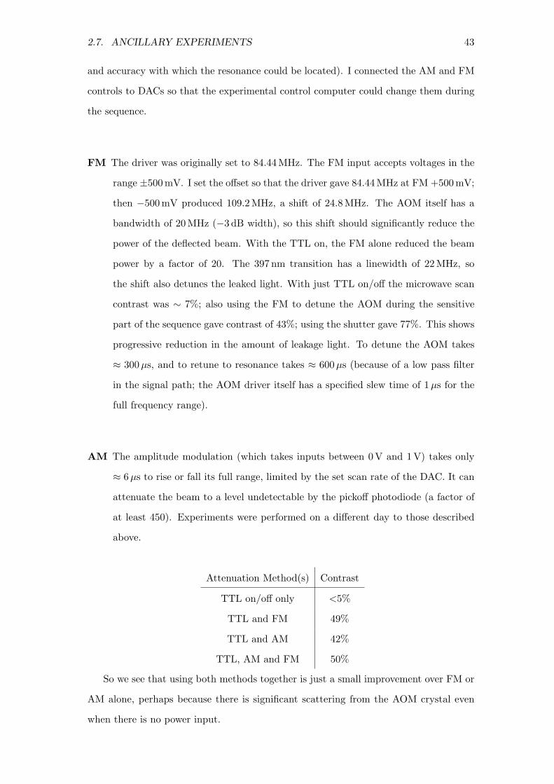
2.7. ANCILLARY EXPERIMENTS 43
and accuracy with which the resonance could be located). I connected the AM and FM
controls to DACs so that the experimental control computer could change them during
the sequence.
FM The driver was originally set to 84.44 MHz. The FM input accepts voltages in the
range ±500 mV. I set the offset so that the driver gave 84.44 MHz at FM +500 mV;
then −500 mV produced 109.2 MHz, a shift of 24.8 MHz. The AOM itself has a
bandwidth of 20 MHz (−3 dB width), so this shift should significantly reduce the
power of the deflected beam. With the TTL on, the FM alone reduced the beam
power by a factor of 20. The 397 nm transition has a linewidth of 22 MHz, so
the shift also detunes the leaked light. With just TTL on/off the microwave scan
contrast was ∼ 7%; also using the FM to detune the AOM during the sensitive
part of the sequence gave contrast of 43%; using the shutter gave 77%. This shows
progressive reduction in the amount of leakage light. To detune the AOM takes
≈ 300 µs, and to retune to resonance takes ≈ 600 µs (because of a low pass filter
in the signal path; the AOM driver itself has a specified slew time of 1 µs for the
full frequency range).
AM The amplitude modulation (which takes inputs between 0 V and 1 V) takes only
≈ 6 µs to rise or fall its full range, limited by the set scan rate of the DAC. It can
attenuate the beam to a level undetectable by the pickoff photodiode (a factor of
at least 450). Experiments were performed on a different day to those described
above.
Attenuation Method(s) Contrast
TTL on/off only <5%
TTL and FM 49%
TTL and AM 42%
TTL, AM and FM 50%
So we see that using both methods together is just a small improvement over FM or
AM alone, perhaps because there is significant scattering from the AOM crystal even
when there is no power input.

44 CHAPTER 2. APPARATUS
2.7.2 850 Polarisation
The 850 nm laser is on a different optical table from the vacuum system, with an optical
fibre carrying light between the tables. The fibre was designed for use at 876 nm [111]
and is monomode and (nominally) polarisation preserving. However, during our work
on readout (Chapter 4), we discovered that the polarisation of light coming from the
fibre varies on a timescale of minutes.
We found that the total power out of the fibre was constant to 0.2%; only the
polarisation varied. But since there was a PBS cube between the fibre output and the
trap, the power seen by the ion did vary, by ∼ 20% as shown in Figure 2.11. The
polarisation of the light entering the fibre was linear, and stable to ∼ 5 mrad, so the
variation must be caused by the fibre.
Figure 2.11 also shows the results of an optical pumping experiment, making a
40Ca+ ion fluoresce with the 397Doppler, 854 and 850 beams. The 850 was set to σ−
polarisation by setting the λ/4 waveplate, shown in Figure 2.12, to +45; both other
beams were linearly polarised as usual. The count rate from the ion was seen to vary over
a timescale of minutes, from ∼ 15 to ∼ 400 counts per second (cps) above background,
with higher counts at lower recorded power. At linear 850 polarisation (i.e. equal σ−
and σ+), the count rate was 16 000 cps.
A rate equations simulation showed that 400 cps can be caused by an extremely low
850 intensity, 0.015 I0. The total power was 18 000 I0 at the times of highest fluorescence,
suggesting that the polarisation impurity is ∼ 8 × 10⁻⁷. This is surprisingly good
given that PBS cubes typically transmit ∼ 10−3 of the incident light of the “wrong”
polarisation [112, Page 679]. By measuring the large PBS, we estimate that it transmits
0.8% of the incident vertically polarised light.
A second, “small” PBS cube was added to the beam path as shown in Figure 2.12.
The optical pumping experiment was repeated: with the waveplate at +45 the fluores-
cence was 60 cps independent of the 850 beam power (figures 2.13). When we set the
waveplate to −45, for σ+ polarisation, the pumping was worse (about 320 cps) and the
count rate was correlated with the Red PD reading (figures 2.14). However the count
rate increased when the PD reading increased which suggests that this might be purely
due to 850 intensity variation at the ion rather than the polarisation changing at the
ion, with the polarisation impurity coming from the waveplate.
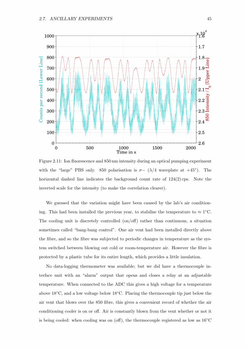
2.7. ANCILLARY EXPERIMENTS 45
0
100
200
300
400
500
600
700
800
900
1000C
ou
nts
per
seco
nd
[L
ow
er
Lin
e]
0 500 1000 1500 2000
1.6
1.7
1.8
1.9
2
2.1
2.2
2.3
2.4
2.5
2.6
x 104
Time in s
85
0 I
nte
nsi
ty /
I0 [
Up
per
Lin
e]
Figure 2.11: Ion fluorescence and 850 nm intensity during an optical pumping experiment
with the “large” PBS only. 850 polarisation is σ− (λ/4 waveplate at +45). The
horizontal dashed line indicates the background count rate of 124(2) cps. Note the
inverted scale for the intensity (to make the correlation clearer).
We guessed that the variation might have been caused by the lab’s air condition-
ing. This had been installed the previous year, to stabilise the temperature to ≈ 1C.
The cooling unit is discretely controlled (on/off) rather than continuous, a situation
sometimes called “bang-bang control”. One air vent had been installed directly above
the fibre, and so the fibre was subjected to periodic changes in temperature as the sys-
tem switched between blowing out cold or room-temperature air. However the fibre is
protected by a plastic tube for its entire length, which provides a little insulation.
No data-logging thermometer was available; but we did have a thermocouple in-
terface unit with an “alarm” output that opens and closes a relay at an adjustable
temperature. When connected to the ADC this gives a high voltage for a temperature
above 18C, and a low voltage below 18C. Placing the thermocouple tip just below the
air vent that blows over the 850 fibre, this gives a convenient record of whether the air
conditioning cooler is on or off. Air is constantly blown from the vent whether or not it
is being cooled: when cooling was on (off), the thermocouple registered as low as 16C
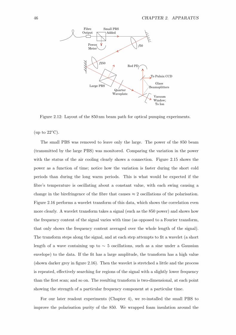
46 CHAPTER 2. APPARATUS
Fibre
OutputSmall PBS
Added
Power
Meterf50
f250
Large PBS
Quarter
Waveplate
Red PD
Vacuum
Window;
To Ion
Glass
Beamsplitters
To Pulnix CCD
Figure 2.12: Layout of the 850 nm beam path for optical pumping experiments.
(up to 22C).
The small PBS was removed to leave only the large. The power of the 850 beam
(transmitted by the large PBS) was monitored. Comparing the variation in the power
with the status of the air cooling clearly shows a connection. Figure 2.15 shows the
power as a function of time; notice how the variation is faster during the short cold
periods than during the long warm periods. This is what would be expected if the
fibre’s temperature is oscillating about a constant value, with each swing causing a
change in the birefringence of the fibre that causes ≈ 2 oscillations of the polarisation.
Figure 2.16 performs a wavelet transform of this data, which shows the correlation even
more clearly. A wavelet transform takes a signal (such as the 850 power) and shows how
the frequency content of the signal varies with time (as opposed to a Fourier transform,
that only shows the frequency content averaged over the whole length of the signal).
The transform steps along the signal, and at each step attempts to fit a wavelet (a short
length of a wave containing up to ∼ 5 oscillations, such as a sine under a Gaussian
envelope) to the data. If the fit has a large amplitude, the transform has a high value
(shown darker grey in figure 2.16). Then the wavelet is stretched a little and the process
is repeated, effectively searching for regions of the signal with a slightly lower frequency
than the first scan; and so on. The resulting transform is two-dimensional, at each point
showing the strength of a particular frequency component at a particular time.
For our later readout experiments (Chapter 4), we re-installed the small PBS to
improve the polarisation purity of the 850. We wrapped foam insulation around the

2.7. ANCILLARY EXPERIMENTS 47
100
125
150
175
200
225
250
275
300
325
350
375
400C
ou
nts
per
seco
nd
[L
ow
er
Lin
e]
1500 2000 2500 3000 3500
1.85
1.9
1.95
2
2.05
2.1
2.15
2.2
2.25
2.3
2.35
2.4
2.45
x 104
Time in s
85
0 I
nte
nsi
ty /
I0 [
Up
per
Lin
e]
Figure 2.13: Ion fluorescence and 850 nm intensity during an optical pumping experiment
with two PBS cubes. 850 polarisation is σ− (λ/4 waveplate at +45). The horizontal
dashed line indicates the background count rate of 109.3(5) cps. The fluorescence has
been smoothed with a moving average filter (covering 24 0.8332 s bins). Note the inverted
scale for the intensity. Figures 2.13 and 2.14 have the same (but shifted) axes scales for
comparison.
fibre where it passed closest to the vent, but power oscillation still occured. Simula-
tions showed the readout process to be insensitive to the 850 intensity, so it was not
worth drastically re-routing the fibre to eliminate the oscillations. It is possible that
slightly adjusting the polarisation of light into the fibre (perhaps making it a better
match to the fibre’s polarisation-maintaining axis) may reduce the variation. However,
in the laboratory next door Gergely Imreh has observed a similar phenomenon in a
polarisation-maintaining fiber at 866 nm despite carefully optimising the input polarisa-
tion [113].
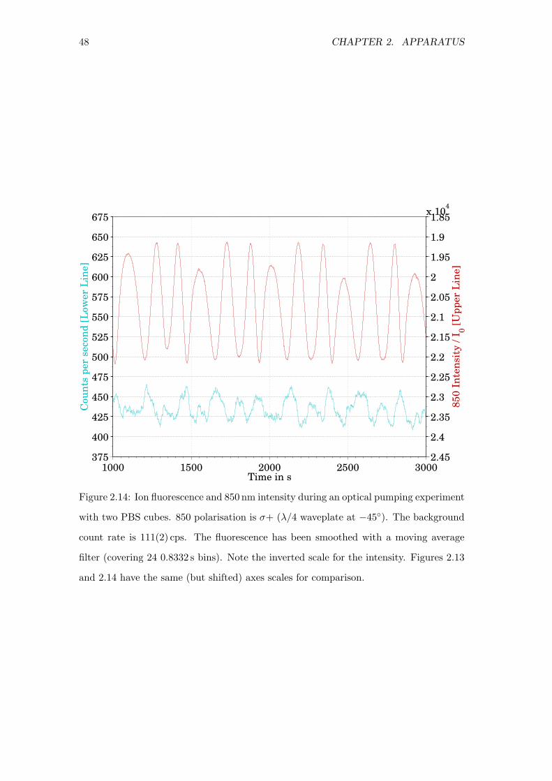
48 CHAPTER 2. APPARATUS
375
400
425
450
475
500
525
550
575
600
625
650
675
Cou
nts
per
seco
nd
[L
ow
er
Lin
e]
1000 1500 2000 2500 3000
1.85
1.9
1.95
2
2.05
2.1
2.15
2.2
2.25
2.3
2.35
2.4
2.45
x 104
Time in s
85
0 I
nte
nsi
ty /
I0 [
Up
per
Lin
e]
Figure 2.14: Ion fluorescence and 850 nm intensity during an optical pumping experiment
with two PBS cubes. 850 polarisation is σ+ (λ/4 waveplate at −45). The background
count rate is 111(2) cps. The fluorescence has been smoothed with a moving average
filter (covering 24 0.8332 s bins). Note the inverted scale for the intensity. Figures 2.13
and 2.14 have the same (but shifted) axes scales for comparison.

2.7. ANCILLARY EXPERIMENTS 49
Time / s
Pow
er /
mV
0 500 1000 1500 2000 2500 3000 3500
1000
1050
1100
1150
1200
1250
1300
1350
1400
Figure 2.15: 850 beam power measured with only the “large” PBS. The red shaded
areas show when the thermocouple has detected cold air from the vents.

50 CHAPTER 2. APPARATUS
Time / s
Wa
vele
t S
ca
le F
acto
r (
arb
. u
nit
s)
0 500 1000 1500 2000 2500 3000 350050
100
150
200
250
300
350
400
Figure 2.16: The 850 power data from figure 2.15 has been wavelet-transformed. The
horizontal axis is time; the vertical axis is period-of-oscillation in arbitrary units, lower
frequency is at the top. The contour plot shows, for each point in time, the magnitude
of each frequency present at that time, where darker is stronger. When the cooling is on
(red hatched areas), the 850 power is varying at higher frequency than when the cooling
is off.
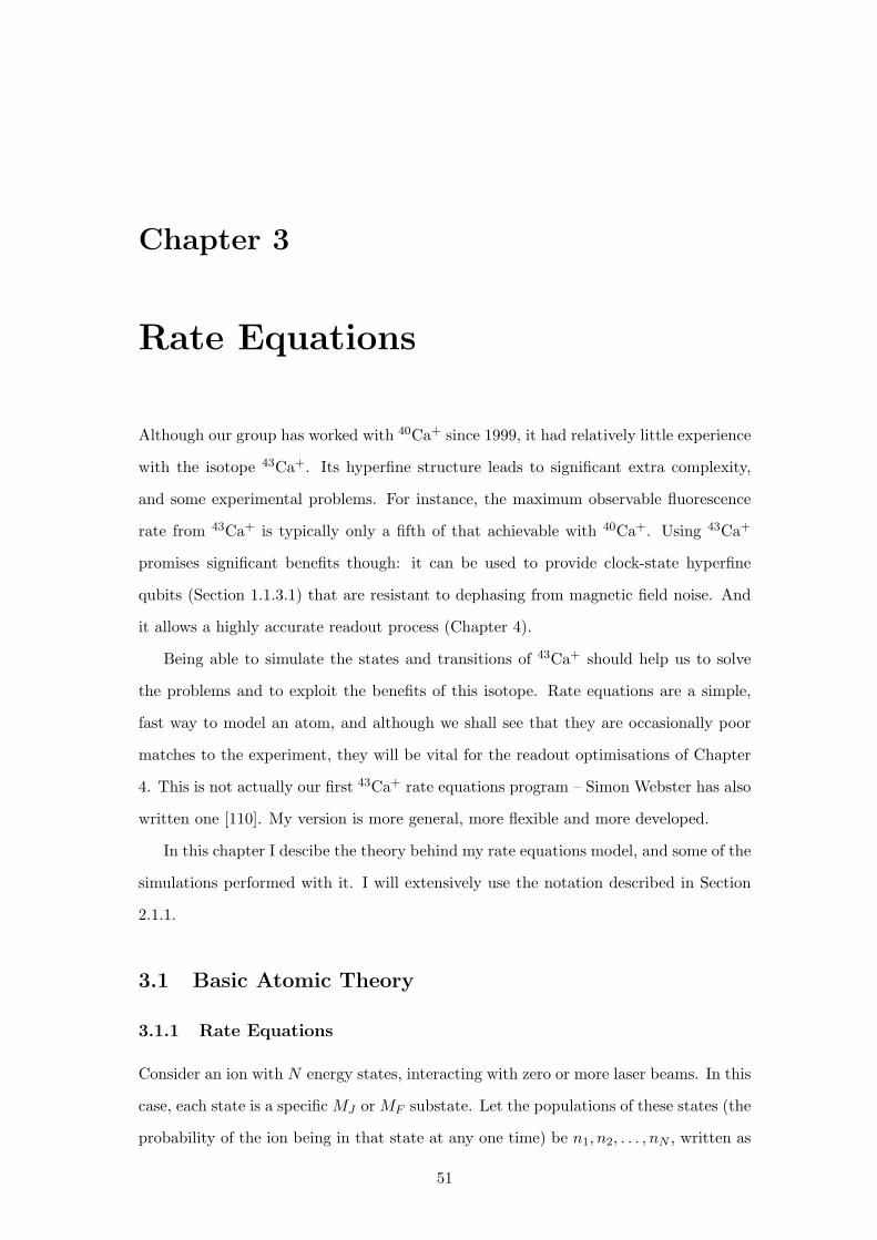
Chapter 3
Rate Equations
Although our group has worked with 40Ca+ since 1999, it had relatively little experience
with the isotope 43Ca+. Its hyperfine structure leads to significant extra complexity,
and some experimental problems. For instance, the maximum observable fluorescence
rate from 43Ca+ is typically only a fifth of that achievable with 40Ca+. Using 43Ca+
promises significant benefits though: it can be used to provide clock-state hyperfine
qubits (Section 1.1.3.1) that are resistant to dephasing from magnetic field noise. And
it allows a highly accurate readout process (Chapter 4).
Being able to simulate the states and transitions of 43Ca+ should help us to solve
the problems and to exploit the benefits of this isotope. Rate equations are a simple,
fast way to model an atom, and although we shall see that they are occasionally poor
matches to the experiment, they will be vital for the readout optimisations of Chapter
4. This is not actually our first 43Ca+ rate equations program – Simon Webster has also
written one [110]. My version is more general, more flexible and more developed.
In this chapter I descibe the theory behind my rate equations model, and some of the
simulations performed with it. I will extensively use the notation described in Section
2.1.1.
3.1 Basic Atomic Theory
3.1.1 Rate Equations
Consider an ion with N energy states, interacting with zero or more laser beams. In this
case, each state is a specific MJ or MF substate. Let the populations of these states (the
probability of the ion being in that state at any one time) be n1, n2, . . . , nN , written as
51
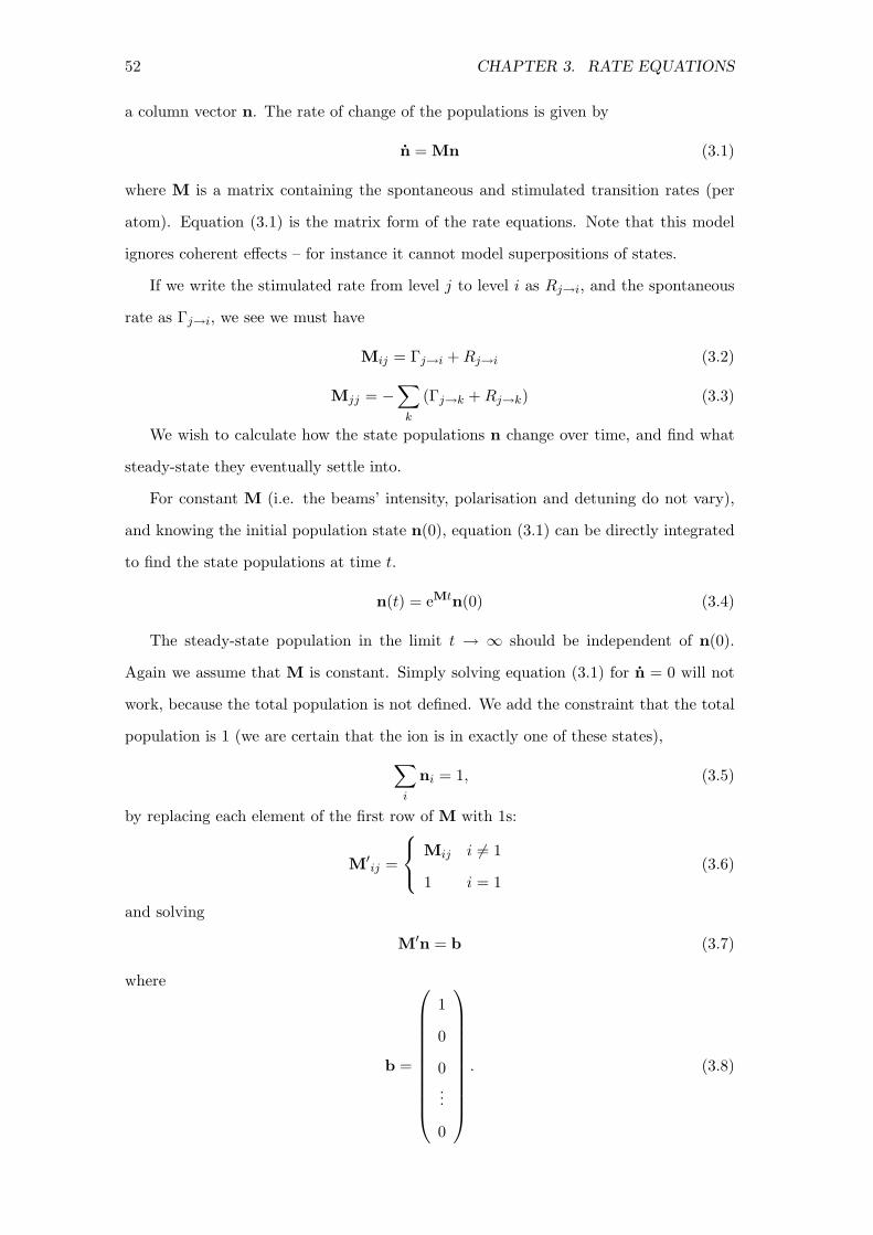
52 CHAPTER 3. RATE EQUATIONS
a column vector n. The rate of change of the populations is given by
n = Mn (3.1)
where M is a matrix containing the spontaneous and stimulated transition rates (per
atom). Equation (3.1) is the matrix form of the rate equations. Note that this model
ignores coherent effects – for instance it cannot model superpositions of states.
If we write the stimulated rate from level j to level i as Rj→i, and the spontaneous
rate as Γj→i, we see we must have
Mij = Γj→i + Rj→i (3.2)
Mjj = −∑
k
(Γj→k + Rj→k) (3.3)
We wish to calculate how the state populations n change over time, and find what
steady-state they eventually settle into.
For constant M (i.e. the beams’ intensity, polarisation and detuning do not vary),
and knowing the initial population state n(0), equation (3.1) can be directly integrated
to find the state populations at time t.
n(t) = eMtn(0) (3.4)
The steady-state population in the limit t → ∞ should be independent of n(0).
Again we assume that M is constant. Simply solving equation (3.1) for n = 0 will not
work, because the total population is not defined. We add the constraint that the total
population is 1 (we are certain that the ion is in exactly one of these states),
∑
i
ni = 1, (3.5)
by replacing each element of the first row of M with 1s:
M′ij =
Mij i 6= 1
1 i = 1(3.6)
and solving
M′n = b (3.7)
where
b =
1
0
0
...
0
. (3.8)
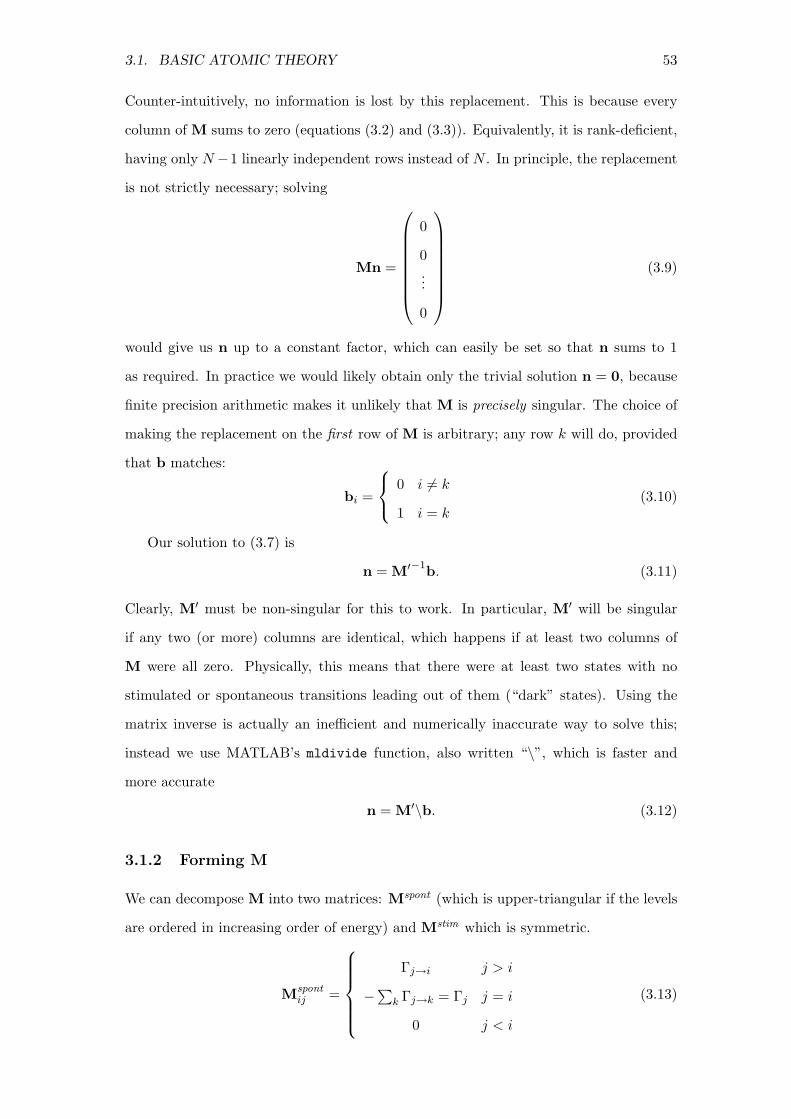
3.1. BASIC ATOMIC THEORY 53
Counter-intuitively, no information is lost by this replacement. This is because every
column of M sums to zero (equations (3.2) and (3.3)). Equivalently, it is rank-deficient,
having only N −1 linearly independent rows instead of N . In principle, the replacement
is not strictly necessary; solving
Mn =
0
0
...
0
(3.9)
would give us n up to a constant factor, which can easily be set so that n sums to 1
as required. In practice we would likely obtain only the trivial solution n = 0, because
finite precision arithmetic makes it unlikely that M is precisely singular. The choice of
making the replacement on the first row of M is arbitrary; any row k will do, provided
that b matches:
bi =
0 i 6= k
1 i = k(3.10)
Our solution to (3.7) is
n = M′−1b. (3.11)
Clearly, M′ must be non-singular for this to work. In particular, M′ will be singular
if any two (or more) columns are identical, which happens if at least two columns of
M were all zero. Physically, this means that there were at least two states with no
stimulated or spontaneous transitions leading out of them (“dark” states). Using the
matrix inverse is actually an inefficient and numerically inaccurate way to solve this;
instead we use MATLAB’s mldivide function, also written “\”, which is faster and
more accurate
n = M′\b. (3.12)
3.1.2 Forming M
We can decompose M into two matrices: Mspont (which is upper-triangular if the levels
are ordered in increasing order of energy) and Mstim which is symmetric.
Mspont
ij =
Γj→i j > i
−∑k Γj→k = Γj j = i
0 j < i
(3.13)

54 CHAPTER 3. RATE EQUATIONS
Mstimij =
Rj→i = Ri→j = Rij j 6= i
−∑k Rj→k j = i(3.14)
3.1.2.1 Electric Dipole Transitions (E1)
The Einstein A coefficient Aji is defined as the total probability per unit time of an
atom in a specific state j making a transition to any of the (2Ji + 1) states of the energy
level i. Aji depends on the quantum numbers n, L and J of the two levels (but not
on the M value of state j, due to isotropy). However we are interested in transitions
where both the initial and final magnetic sub-states are specific. The selection rules
and matrix elements depend on Clebsch-Gordon coefficients, here represented using 3-j
symbols (definitions and tables can be found in Cowan [114, Chapter 5 and Appendix
C]). Letting j and i represent specific states, the spontaneous transition rate is [110]
Γj→i = Aij(2Jj + 1)
Ji 1 Jj
−MJ,i q MJ,j
2
(3.15)
where q = MJ,i −MJ,j represents the polarisation of the emitted photon: 0 for a photon
linearly polarised parallel to the z-axis (π); +1 for a photon circularly polarised clockwise
(as seen from the positive z direction, for a photon emitted in that direction) (σ+); −1
for anticlockwise circular polarisation (σ−). The 3-j symbol is zero unless its bottom
row sums to zero – this selects for conservation of angular momentum.
When discussing transitions between hyperfine levels, rather than fine structure lev-
els, an additional factor involving a 6-j symbol is needed [114, Appendix D]. We need
to include the nuclear spin I in the formula (I = 7/2 for calcium-43), and work with
F = J + I as the ion’s total spin operator. The result is [110]
Γj→i = Aij(2Jj + 1)(2Fi + 1)(2Fj + 1)
×
Fi 1 Fj
−MF,i q MF,j
2
Ji I Fi
Fj 1 Jj
2
(3.16)
My MATLAB routines calculate the 3-j and 6-j symbols using “threej.m” and “sixj.m”
(both written by Simon Webster). The 3-j and 6-j symbols are highly symmetrical in
their inputs: for example the 3-j symbol is invariant under any cyclic permutation of its
columns, and the 6-j symbol is invariant under any permutation of its columns.
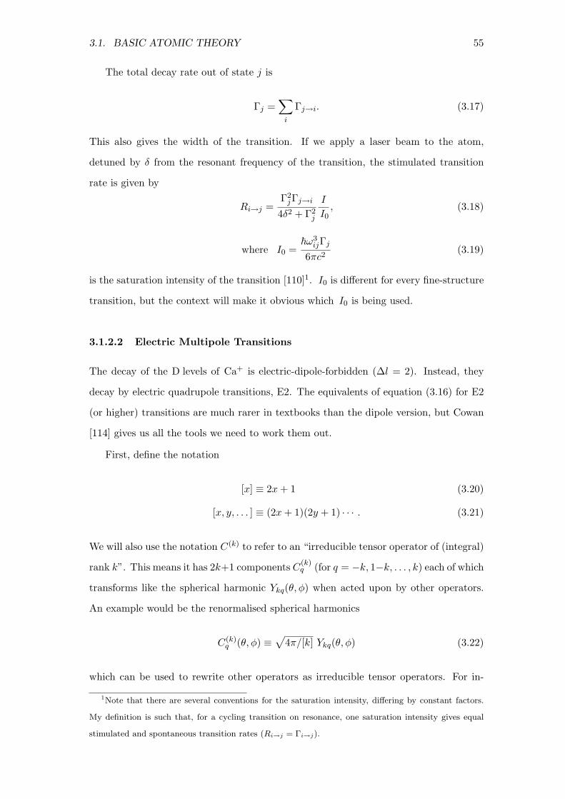
3.1. BASIC ATOMIC THEORY 55
The total decay rate out of state j is
Γj =∑
i
Γj→i. (3.17)
This also gives the width of the transition. If we apply a laser beam to the atom,
detuned by δ from the resonant frequency of the transition, the stimulated transition
rate is given by
Ri→j =Γ2
jΓj→i
4δ2 + Γ2j
I
I0, (3.18)
where I0 =~ω3
ijΓj
6πc2(3.19)
is the saturation intensity of the transition [110]1. I0 is different for every fine-structure
transition, but the context will make it obvious which I0 is being used.
3.1.2.2 Electric Multipole Transitions
The decay of the D levels of Ca+ is electric-dipole-forbidden (∆l = 2). Instead, they
decay by electric quadrupole transitions, E2. The equivalents of equation (3.16) for E2
(or higher) transitions are much rarer in textbooks than the dipole version, but Cowan
[114] gives us all the tools we need to work them out.
First, define the notation
[x] ≡ 2x + 1 (3.20)
[x, y, . . . ] ≡ (2x + 1)(2y + 1) · · · . (3.21)
We will also use the notation C(k) to refer to an “irreducible tensor operator of (integral)
rank k”. This means it has 2k+1 components C(k)q (for q = −k, 1−k, . . . , k) each of which
transforms like the spherical harmonic Ykq(θ, φ) when acted upon by other operators.
An example would be the renormalised spherical harmonics
C(k)q (θ, φ) ≡
√
4π/[k] Ykq(θ, φ) (3.22)
which can be used to rewrite other operators as irreducible tensor operators. For in-
1Note that there are several conventions for the saturation intensity, differing by constant factors.
My definition is such that, for a cycling transition on resonance, one saturation intensity gives equal
stimulated and spontaneous transition rates (Ri→j = Γi→j).

56 CHAPTER 3. RATE EQUATIONS
stance, a vector operator
r =
rx
ry
rz
=
r sin(θ) cos(φ)
r sin(θ) sin(φ)
r cos(θ)
(3.23)
becomes [114, Section 11-3]
r(1) = rC(1) (3.24)
where
r(1)1 = − 1√
2(rx + iry) = − r√
2sin(θ)eiφ
r(1)0 = rz = r cos(θ)
r(1)−1 =
1√2
(rx − iry) =r√2
sin(θ)e−iφ
(3.25)
are its components. If we assume r is the position operator of the outer electron of
Ca+, we immediately see that the electric dipole operator is also an irreducible tensor
operator
P (1) = −er(1) = −erC(1) (3.26)
as is the electric quadrupole operator
P (2) = −er(2) = −er2C(2). (3.27)
We will need the Wigner-Eckart Theorem: let T (k) be any irreducible tensor operator
acting in a space spanned by basis functions |αjm〉. These are eigenstates of J2 with
value j(j + 1), and Jz with value m, with α representing all other quantum numbers.
Then commutation relations between J± and T(k)q imply that [114, Section 11-4]
⟨
αjm∣
∣T (k)q
∣
∣α′j′m′⟩
= (−1)j−m
j k j′
−m q m′
⟨
αj∥
∥T (k)∥
∥α′j′⟩
(3.28)
where⟨
αj∥
∥T (k)∥
∥α′j′⟩
is a reduced matrix element and contains the rest of the physics
such as wavefunction overlap.
Now consider the product of two tensor operators, T (kt) and W (kw). Let
V(K)Q ≡ (T (kt) × W (kw))
(K)Q (3.29)
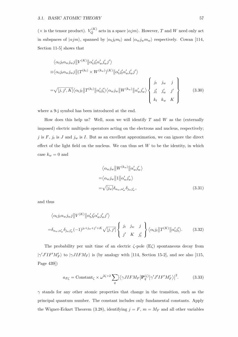
3.1. BASIC ATOMIC THEORY 57
(× is the tensor product). V(K)Q acts in a space |αjm〉. However, T and W need only act
in subspaces of |αjm〉, spanned by |αtjtmt〉 and |αwjwmw〉 respectively. Cowan [114,
Section 11-5] shows that
⟨
αtjtαwjwj∥
∥V (K)∥
∥α′tj
′tα
′wj′wj′
⟩
≡⟨
αtjtαwjwj∥
∥(T (kt) × W (kw))(K)∥
∥α′tj
′tα
′wj′wj′
⟩
=√
[j, j′, K]⟨
αtjt
∥
∥T (kt)∥
∥α′tj
′t
⟩⟨
αwjw
∥
∥W (kw)∥
∥α′wj′w
⟩
jt jw j
j′t j′w j′
kt kw K
(3.30)
where a 9-j symbol has been introduced at the end.
How does this help us? Well, soon we will identify T and W as the (externally
imposed) electric multipole operators acting on the electrons and nucleus, respectively;
j is F , jt is J and jw is I. But as an excellent approximation, we can ignore the direct
effect of the light field on the nucleus. We can thus set W to be the identity, in which
case kw = 0 and
⟨
αwjw
∥
∥W (kw)∥
∥α′wj′w
⟩
=⟨
αwjw
∥
∥1∥
∥α′wj′w
⟩
=√
[jw]δαw,α′wδjwj′w , (3.31)
and thus
⟨
αtjtαwjwj∥
∥V (K)∥
∥α′tj
′tα
′wj′wj′
⟩
=δαw,α′wδjwj′w(−1)jt+jw+j′+K
√
[j, j′]
jt jw j
j′ K j′t
⟨
αtjt
∥
∥T (K)∥
∥α′tj
′t
⟩
. (3.32)
The probability per unit time of an electric ζ-pole (Eζ) spontaneous decay from
|γ′J ′IF ′M ′F 〉 to |γJIFMF 〉 is (by analogy with [114, Section 15-2], and see also [115,
Page 439])
aEζ = Constantζ × ω2ζ+2∑
q
∣
∣
⟨
γJIFMF
∣
∣P(ζ)q
∣
∣γ′J ′IF ′M ′F
⟩∣
∣
2. (3.33)
γ stands for any other atomic properties that change in the transition, such as the
principal quantum number. The constant includes only fundamental constants. Apply
the Wigner-Eckart Theorem (3.28), identifying j = F , m = MF and all other variables

58 CHAPTER 3. RATE EQUATIONS
as α:
aEζ = Constantζ × ω2ζ+2∑
q
F ζ F ′
−MF q M ′F
2
×∣
∣
⟨
γJIF∥
∥P(ζ)∥
∥γ′J ′IF ′⟩∣
∣
2. (3.34)
Now we can use equation (3.32). Identify j = F , jt = J , jw = I, V(K) = T(K) = P(ζ);
set jw = j′w and αw = α′w because the light doesn’t couple to the nuclear spin; and we
obtain
aEζ = Constantζ × ω2ζ+2∑
q
F ζ F ′
−MF q M ′F
2
[F, F ′]
×
J I F
F ′ ζ J ′
2
∣
∣
⟨
γJ∥
∥P(ζ)∥
∥γ′J ′⟩∣
∣
2. (3.35)
It turns out that
∣
∣
⟨
γJ∥
∥P(ζ)∥
∥γ′J ′⟩∣
∣
2 × Constantζ × ω2ζ+2 = [J ′]A (3.36)
where A is the relevant Einstein A Coefficient. So
aEζ =∑
q
F ζ F ′
−MF q M ′F
2
[F, F ′, J ′]
J I F
F ′ ζ J ′
2
A (3.37)
which, setting ζ → 2, is the formula I use in my programs.
3.1.2.3 Magnetic Dipole Transitions (M1)
While a complete treatment of this subject would also consider magnetic dipole (and
perhaps magnetic multipole) transitions, they are not necessary for calculations with
Ca+. Sahoo et al. [15] calculated the lifetimes of the 3D levels of Ca+ using relativistic
coupled-cluster theory. M1 transitions are allowed from D3/2 → S1/2 and from D5/2 →
D3/2, but in both cases they make only very small contributions to the levels’ lifetimes.
For the former transition the M1 reduced matrix element is only 10−4 times the strength
of the E2 element; and the D5/2 → D3/2 M1 transition is suppressed because of the small
energy difference and the ω3 factor in the transition rate (its Einstein A coefficient is
calculated to be only 2.4 × 10⁻⁶ s−1 [116]). In Ba+, though, the D5/2 → D3/2 reduces
the lifetime of D5/2 by 16% compared to the E2 decay alone.

3.1. BASIC ATOMIC THEORY 59
3.1.3 Hyperfine Energy Shifts
Because the rate of a stimulated transition depends on the laser detuning δ, it is im-
portant to be able to accurately calculate the energy spacing of all the states. In 40Ca+
(which has zero nuclear spin I), the spacings are determined by the fine structure of
the ion, and the Zeeman shifts of individual states. 43Ca+ is the only stable isotope of
calcium with non-zero nuclear spin: I = 7/2. We will only be concerned with two ways
that the electrons’ wavefunctions can interact with the nucleus – the nucleus’s magnetic
dipole moment and its electric quadrupole moment2.
The effect of those moments is given by Woodgate [119, Second Edition, Section 9.5]:
Let K = F (F + 1) − J(J + 1) − I(I + 1) (3.38)
Then ∆E =AL,J
2K +
BL,J
4
32K(K + 1) − 2I(I + 1)J(J + 1)
I(2I − 1)J(2J − 1)(3.39)
where AL,J and BL,J are the hyperfine structure constants for the magnetic dipole and
electric quadrupole interactions respectively, and depend only on L and J (for a given
isotope). BL,J = 0 for J < 1 or I < 1. ∆E is the energy shift of a state relative to the
centre-of-gravity of a level. That is,
∑
F,MF
∆EL,J,F,MF= 0 ∀L, J. (3.40)
AL,J is not to be confused with an Einstein A coefficient! These energy shifts are plotted
in Appendix A.
The Zeeman energy shift due to an external magnetic field B is given by
∆EZ = gF MF µBB (3.41)
= gJ
(
F (F + 1) + J(J + 1) − I(I + 1)
2F (F + 1)
)
MF µBB (3.42)
=
(
3J(J + 1) + S(S + 1) − L(L + 1)
2J(J + 1)
)
×(
F (F + 1) + J(J + 1) − I(I + 1)
2F (F + 1)
)
MF µBB. (3.43)
This neglects the direct interaction between the nuclear moments and B; and is valid only
in the limit of low magnetic field when ∆EZ ≪ ∆E. This condition is generally fulfilled
2The nucleus’s electric dipole moment, and other odd electric moments and even magnetic moments,
are very close to zero. They would be precisely zero if either parity-reversal or time-reversal symmetries
held exactly; Weak interactions violate these symmetries but the effect is still unmeasurably small [117,
Section 2.2.8], even to specialised experiments [118].
60 CHAPTER 3. RATE EQUATIONS
in the experiments and simulations in this work. The exception is the D5/2 level, where
the Zeeman shifts become non-linear even for our typical fields of ∼ 2×10⁻⁴ T; however
my programs still use the linear model because the precise splittings are unimportant for
this work. Note that the formula (3.43) is still valid for isotopes with no nuclear spin –
the second bracketed term in the product becomes 1 when I = 0 and F ≡ J . Quantum
electrodynamic effects lead to gJ deviating from(
3J(J+1)+S(S+1)−L(L+1)2J(J+1)
)
, and for some
levels these have been measured to high precision as shown in Table 3.1. I do not use
these measurements and simply use the formula (3.43).
3.2 The Transitions Suite
“Transitions” is my suite of MATLAB functions. Their main purpose was to allow rate-
equations simulations of 43Ca+, although they include routines to calculate intermediate-
field Zeeman shifts and light shifts. They are written to be relatively general: simply
by changing one settings file, they can simulate other alkaline earth ions (e.g. Sr+),
neutral alkaline atoms (e.g. Rb) or other similar one-electron systems. Note however
that capability for M1 transitions may need to be added to work with species such as Ba+
(Section 3.1.2.3). The programs will not necessarily work with multi-electron systems
such as neutral alkaline earth atoms – this is because I have assumed the electron’s spin
S is 12 throughout. I have also assumed that the fine-structure splitting is always small
enough that levels with the same value of n and L, but different Js, are adjacent when
the levels are ordered by energy.
The detailed implementation of the model is described in the users’ manual in Ap-
pendix B.
3.3 Atomic Constants
These are some of the relevant atomic data for Ca+. Here I list the most precise values
I could find at the time of writing; early simulations may have been performed with less
precise numbers.
Nuclear Spin This is zero for all isotopes except 43Ca+, which has I = 72 .

3.3. ATOMIC CONSTANTS 61
Levels Each fine-structure level is listed separately and manually. They are identified
by their principal quantum number n, orbital angular momentum L and total angular
momentum J . n is not used in any calculations: its purpose is only to distinguish
between different levels with the same L and J , if such a situation were ever needed. For
each such level is recorded its hyperfine A and B coefficients. These are obviously non-
zero only for 43Ca+, and are recorded in Table 3.1. I also include gyromagnetic factors
gJ , if they have been measured, for reference only (currently my program calculates
them from the quantum numbers using Equation (3.43)).
Level A / MHz B / MHz Ref. gJ Ref.
4S1/2 −806.402 071 60(8) 0 [120] 2.002 256 64(9) [17]
4P1/2 −145.4(1) 0 [16]
4P3/2 −31.0(2) −6.9(1.7) [16]
3D3/2 −47.3(2) −3.7(1.9) [16]
3D5/2 −3.8(6) −3.9(6.0) [16]
3D5/2 −3.893 1(2) −4.241(4) [121, 122] 1.200 334 0(3) [123]
Table 3.1: The hyperfine structure constants for 43Ca+, and gyromagnetic ratios for
Ca+ in general. The more precise values for D5/2 were published after many of the
results in this thesis were calculated.
Transitions Transitions between hyperfine- or fine-structure-split levels are ignored
(there is no P3/2 → P1/2 for instance). Each transition we want to include is labeled by
the n, L and J values of the upper and lower levels, and for each I include its Einstein A
coefficient, the wavelength and the isotope shift between the same transition in 43Ca+
and 40Ca+. The same array is used to store the saturation intensity of the transition,
although this is calculated by the setup function rather than specified as a parameter.
The wavelength and isotope shift are stored in this array for reference and ease of access,
although they are not directly used in calculations. Table 3.2 shows the data.

62C
HA
PT
ER
3.
RA
TE
EQ
UA
TIO
NS
Transition Wavenumber Wavelength Frequency Ref. Isotope Shift Ref. Einstein A Ref. Saturation
/ cm−1 / nm / THz / MHz Coefficient / s−1 Intensity / W m−2
4S1/2 → 4P1/2 25 191.519 87(6) 396.958 978 8(9) 755.222 766 2(17) [21] 688(17) [106] 132 × 106 933.82
4S1/2 → 4P3/2 25 414.415 62(2) 393.477 471 6(3) 761.905 012 7(5) [124] 692(19) [106] 135.0(4) × 106 [20] 987.58
3D3/2 → 4P1/2 11 541.32 866.452 346.000 [125, 126] -3464.3(3.0) [16] 8.4 × 10⁶ 89.798
3D3/2 → 4P3/2 11 764.21 850.036 352.682 [125, 126] -3462.4(2.6) [16] 0.955(6) × 106 [20] 97.954
3D5/2 → 4P3/2 11 703.52 854.444 350.863 [125, 126] -3465.4(3.7) [16] 8.48(4) × 106 [20] 96.446
4S1/2 → 3D5/2 137 10.889 610 718 40(3) 729.347 276 793 955(2) 411.042 129 776 393 2(10) [123] 4134.713(5) [121] 0.856(5) [55] 9.181 × 10⁻⁷
4S1/2 → 3D3/2 13 650.19 732.591 409.222 [125, 126] 0.850(8) [98] 8.818 × 10⁻⁷
Table 3.2: Properties of the transitions between energy levels in 40Ca+. The isotope shift is νCentre of Gravity, Ca-43 − νCa-40.
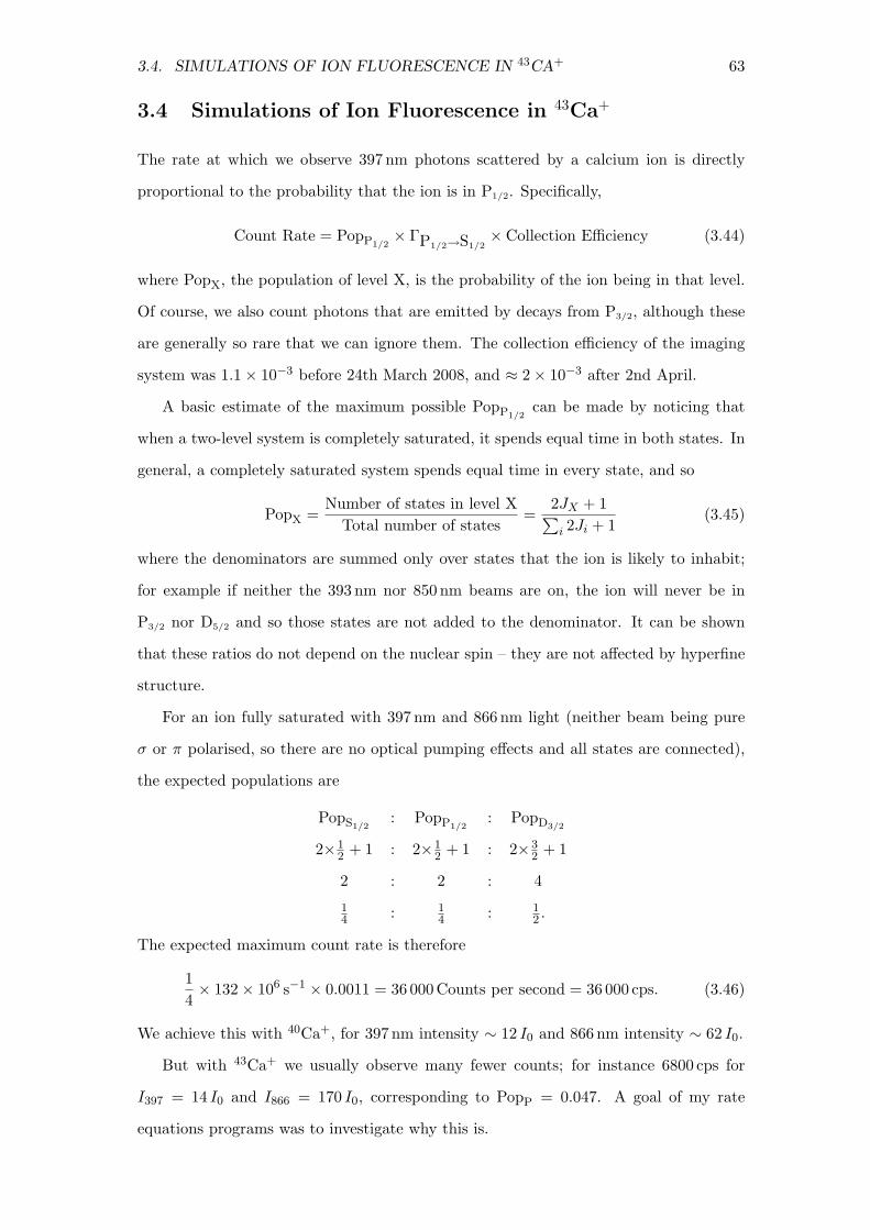
3.4. SIMULATIONS OF ION FLUORESCENCE IN 43CA+ 63
3.4 Simulations of Ion Fluorescence in 43Ca+
The rate at which we observe 397 nm photons scattered by a calcium ion is directly
proportional to the probability that the ion is in P1/2. Specifically,
Count Rate = PopP1/2× ΓP1/2→S1/2
× Collection Efficiency (3.44)
where PopX, the population of level X, is the probability of the ion being in that level.
Of course, we also count photons that are emitted by decays from P3/2, although these
are generally so rare that we can ignore them. The collection efficiency of the imaging
system was 1.1 × 10⁻³ before 24th March 2008, and ≈ 2 × 10⁻³ after 2nd April.
A basic estimate of the maximum possible PopP1/2can be made by noticing that
when a two-level system is completely saturated, it spends equal time in both states. In
general, a completely saturated system spends equal time in every state, and so
PopX =Number of states in level X
Total number of states=
2JX + 1∑
i 2Ji + 1(3.45)
where the denominators are summed only over states that the ion is likely to inhabit;
for example if neither the 393 nm nor 850 nm beams are on, the ion will never be in
P3/2 nor D5/2 and so those states are not added to the denominator. It can be shown
that these ratios do not depend on the nuclear spin – they are not affected by hyperfine
structure.
For an ion fully saturated with 397 nm and 866 nm light (neither beam being pure
σ or π polarised, so there are no optical pumping effects and all states are connected),
the expected populations are
PopS1/2: PopP1/2
: PopD3/2
2×12 + 1 : 2×1
2 + 1 : 2×32 + 1
2 : 2 : 4
14 : 1
4 : 12 .
The expected maximum count rate is therefore
1
4× 132 × 106 s−1 × 0.0011 = 36 000 Counts per second = 36 000 cps. (3.46)
We achieve this with 40Ca+, for 397 nm intensity ∼ 12 I0 and 866 nm intensity ∼ 62 I0.
But with 43Ca+ we usually observe many fewer counts; for instance 6800 cps for
I397 = 14 I0 and I866 = 170 I0, corresponding to PopP = 0.047. A goal of my rate
equations programs was to investigate why this is.

64 CHAPTER 3. RATE EQUATIONS
An early question is whether the lasers are tuned to the correct frequency. The
397 nm Doppler cooling laser must excite out of both the S31/2 and S4
1/2 hyperfine man-
ifolds. These are so far apart (3226 MHz compared to the 397 nm transition’s natural
linewidth of 22 MHz, Figure 2.1) that the fluorescence rate will almost vanish unless
sidebands are added to the beam, e.g. with an EOM. There are several choices for the
beam’s detuning and modulation. The carrier can address any one of the four transi-
tions, and a sideband can address either of the two transitions that excite from the other
S1/2 manifold (the other sideband is wasted). A rate equations fluorescence calculation
is shown in Figure 3.1 that simulates each of these eight choices. I assume parameters
(laser intensity, polarisation, sideband power distribution etc.) similar to the experi-
ment that found PopP = 0.047 – that result is marked on the graph for reference. The
simulation shows the P1/2 population as a function of 866 nm detuning – the experiment
was also a scan of this laser, and the 4.7% result was the peak of this scan.
It can be seen that the simulation achieves P populations above 7%, somewhat higher
than the experiment. Note that the count rate should increase slightly if we tuned the
397 nm carrier and sideband to S41/2 → P3
1/2 and S31/2 → P4
1/2. But the S41/2 → P3
1/2
transition is less than 600 MHz blue of the S41/2 → P4
1/2 line, so having a laser component
at that frequency would run a slightly higher risk of Doppler-heating the ion. We thus
prefer to use S41/2 → P4
1/2 and S31/2 → P4
1/2 as marked on the plot.
Depending on the P1/2 F -manifold(s) to which the 397 excites, the 866 will need
to repump from different D3/2 manifolds at different rates (for instance, if the 397 does
not excite to P31/2 then the ion will rarely fall into D2
3/2). Since the 866 hyperfine com-
ponents vary in strength (see Figure A.2, but note that that figure uses the opposite
labelling convention to Figure 3.1), the optimal 866 detuning depends on the choice of
397 frequencies.
The experiment required the ion to be continuously Doppler cooled by the lasers, so
the 397 nm carrier was red-detuned from resonance by approximately 12 MHz and the
sideband by 6 MHz. Feeding this into the simulation does indeed reduce PopP, but not
enough to match the experiment. The problem can be seen by comparing the simulation
with the actual data from the experimental scan, in Figure 3.3. We immediately see
three sharp dips in the experimental data: dark resonances. Dark resonances (also
known as electromagnetically induced transparency or coherent population trapping)
occur in a three-level system when the two laser beams have the same detuning (as

3.4. SIMULATIONS OF ION FLUORESCENCE IN 43CA+ 65
−1500 −1000 −500 0 500 1000 1500 20000
0.01
0.02
0.03
0.04
0.05
0.06
0.07
0.08
866 Frequency Relative to Centre of Gravity / MHz
Pop
ula
tion
of
P1
/2
Carrier on S1/2
3→ P
1/2
4; Sideband on S
1/2
4→ P
1/2
4
Carrier on S1/2
3→ P
1/2
4; Sideband on S
1/2
4→ P
1/2
3
Carrier on S1/2
3→ P
1/2
3; Sideband on S
1/2
4→ P
1/2
4
Carrier on S1/2
3→ P
1/2
3; Sideband on S
1/2
4→ P
1/2
3
Carrier on S1/2
4→ P
1/2
4; Sideband on S
1/2
3→ P
1/2
4 *
Carrier on S1/2
4→ P
1/2
3; Sideband on S
1/2
3→ P
1/2
4
Carrier on S1/2
4→ P
1/2
4; Sideband on S
1/2
3→ P
1/2
3
Carrier on S1/2
4→ P
1/2
3; Sideband on S
1/2
3→ P
1/2
3
Experimental P Population: 4.7%
3→44→4
5→42→3
3→34→3
Figure 3.1: Rate equations simulation of ion fluorescence as a function of 866 nm beam
detuning, for a variety of detunings and sideband modulations of the 397 nm beam.
I397 = 14 I0; Sideband:Carrier:Sideband intensity splitting = 13:74:13; I866 = 170 I0;
both beams are equally split between σ− and σ+ polarisations. This attempts to repli-
cate the experiment that produced maximum PopP of 4.7%; in the experiment the carrier
was tuned to S41/2 → P4
1/2, sideband to S31/2 → P4
1/2 (starred on plot). Here the 397 nm
components are set to be exactly resonant with the stated transitions. Solid/dotted
lines of the same colour show 397 choices that address the same transitions, but with
sidband and carrier swapped. Vertical lines show positions of the hyperfine components
of D3/2 → P1/2, labeled Flower → Fupper.

66 CHAPTER 3. RATE EQUATIONS
shown in Figure 3.2). One of the resulting dressed states contains only S1/2 and D3/2
and does not scatter photons. The ion then falls into the dark state by optical pumping.
S1/2
39
7n
m
86
6n
mD3/2
P1/2
δr δb
Figure 3.2: Three-level system representing the 397 nm and 866 nm transitions. A dark
resonance occurs when the detunings are equal: δb = δr.
Optical pumping to dark states can occur even when the two-beam resonance condi-
tion is not met. The most obvious situation is when pure circularly polarised (say, σ+)
397 nm light is applied to 43Ca+. No such transition exists from the state S4,+41/2 so that
state is dark and the ion will be optically pumped into it, no matter what is happening
on the 866 nm transition. If the laser is changed to any other polarisation, there exists
a superposition of Zeeman-states that is dark, and again the ion will eventually fall into
that state. In our experiment we apply a magnetic field to the ions. This field lifts
the degeneracy of the states, so the dark state is no longer stable and the ion precesses
out of it. However, the precession is relatively slow and so the fluorescence rate is still
reduced.
Dark states and resonances cannot in general be calculated using rate equations,
because they depend on coherent interactions between states and light fields that rate
equations do not include. Including coherences leads to the Bloch equations. Berkeland
and Boshier have used Bloch equations to study dark states, and methods for desta-
bilising them [127]. They consider modulations δ being applied to the system either
by magnetic field (in which δ is the Zeeman shift between states) or by modulation
of the polarisation of the laser (δ is the product of the modulation frequency and the
amplitude of the phase shift imparted between the polarisation components). Typically
they found that the fluorescence rate was maximised when δ was about half the Rabi
frequency Ω of a laser-stimulated transition; δ ≪ Ω allowed the system to spend too
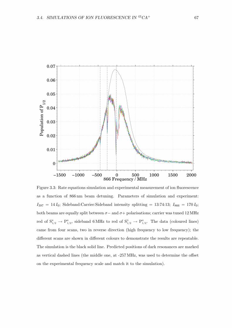
3.4. SIMULATIONS OF ION FLUORESCENCE IN 43CA+ 67
−1500 −1000 −500 0 500 1000 1500 2000
0
0.01
0.02
0.03
0.04
0.05
0.06
0.07
866 Frequency / MHz
Pop
ula
tion
of
P1
/2
Figure 3.3: Rate equations simulation and experimental measurement of ion fluorescence
as a function of 866 nm beam detuning. Parameters of simulation and experiment:
I397 = 14 I0; Sideband:Carrier:Sideband intensity splitting = 13:74:13; I866 = 170 I0;
both beams are equally split between σ− and σ+ polarisations; carrier was tuned 12 MHz
red of S41/2 → P4
1/2, sideband 6 MHz to red of S31/2 → P4
1/2. The data (coloured lines)
came from four scans, two in reverse direction (high frequency to low frequency); the
different scans are shown in different colours to demonstrate the results are repeatable.
The simulation is the black solid line. Predicted positions of dark resonances are marked
as vertical dashed lines (the middle one, at -257 MHz, was used to determine the offset
on the experimental frequency scale and match it to the simulation).
68 CHAPTER 3. RATE EQUATIONS
much time in the dark state for strong fluorescence, and δ ≫ Ω corresponded to the
laser being too far detuned. However, in systems with large angular momenta (such as
43Ca+) the fluorescence rate is relatively independent of δ [127, Section IV.C.].
In the experiment above, the Rabi frequencies of both the 397 nm and 866 nm tran-
sitions were ∼ 20 MHz, compared to Zeeman shifts of 0.6 MHz in S1/2, 0.2 MHz in P1/2
and ∼ 0.6 MHz in D3/2. Although we are in the regime of δ ≪ Ω we have been unable
to improve 43Ca+ count rates by reducing either laser intensity, presumably an effect of
the large number of states. In 40Ca+, however, count rate is maximised for an 866 nm
intensity of ∼ 30 I0. 40Ca+ has the additional benefit that the 397 nm transition is
Ji → Jj for Ji = Jj and Ji being a half-integer – in this case there are no dark states
except for pure σ polarisation [127].
The first-order Zeeman splitting of a manifold vanishes when F (F + 1) + J(J + 1) =
I(I + 1) (3.43). In 43Ca+ this happens when F = 3 and J = 3/2. δ is thus extremely
small for D33/2, and we may worry that this allows a dark state to easily form. A
crude simulation can be performed in rate equations, simply by setting the D33/2 → P3
1/2
transition rate to zero. We do not eliminate D33/2 → P4
1/2; there is no dark state for any
polarisation when the upper level has higher angular momentum than the lower. Figure
3.4 repeats Figure 3.3 with just this change, and we see that total elimination is overly
pessimistic. In practice the existence of the D33/2 → P4
1/2 transition partially prevents
the dark state becoming established.
Attempts have been made to follow the other recommendation of Berkeland and
Boshier [127]; polarisation modulation. A second 866 nm beam, and a second 397 nm
beam, both derived from separate lasers, were focussed on the ion with different polari-
sations and frequencies to the usual beams. The effect should have been for the ion to
feel a light field of constantly changing polarisation, destabilising the dark states and
increasing fluorescence. However, no improvement was found. The Innsbuck group has
also noted that 43Ca+ produces fewer counts than 40Ca+ [128]. Their 866 nm beam
has three frequency components, at 145 MHz and 390 MHz above the lowest component;
then they split the beam into two, and direct them to the ion at perpendicular directions
[129]. It is claimed that this increases the fluorescence, although no further details are
given.

3.4. SIMULATIONS OF ION FLUORESCENCE IN 43CA+ 69
−1500 −1000 −500 0 500 1000 1500 2000
0
0.01
0.02
0.03
0.04
0.05
0.06
0.07
866 Frequency / MHz
Pop
ula
tion
of
P1
/2
Unsilenced
3→3 Silenced
Figure 3.4: A repeat of Figure 3.3, except that the dashed curve shows the result of
setting the D33/2 → P3
1/2 transition rate to zero.
3.4.1 Bloch Equations
Derek Stacey is currently constructing a detailed Bloch equations model of 43Ca+. Our
group has previously used Bloch equations to study 40Ca+ [108], but the odd isotope is
considerably more challenging. There are 64 states in total in S1/2, P1/2 and D3/2, and
a rate equations model needs to work with 64-by-64 matrices for this system. Bloch
equations use the density matrix of the system, that is itself a 64-by-64 matrix; the
transitions thus (in principle) involve matrices with 644 = 16 777 216 elements. Many
fewer are needed in practice because the transitions matrix is highly sparse; if the
situation is simplified to include no π polarised light, there are 17 286 non-vanishing
matrix elements [130]. This is a tractable computer calculation. The simulation has
been tested against fluorescence data I recorded from the ion – an example is shown in
Figure 3.5.
A long-standing idea for improving the fluorescence is to add sidebands to the 866 nm
beam, allowing it to bridge some of the hyperfine structure in that transition. When
this was tried the result was highly dependent on the 866 nm detuning, having a forest

70 CHAPTER 3. RATE EQUATIONS
−1000 −800 −600 −400 −200 0 200 400 600 8000
0.005
0.01
0.015
0.02
0.025
0.03
866 Frequency / MHz
Pop
ula
tion
of
P1
/2
Bloch Equations
Rate Equations
Figure 3.5: Rate equations and Bloch equations simulations, and experimental mea-
surement, of ion fluorescence as a function of 866 nm beam detuning. The Bloch equa-
tions curve was fitted to the data in a least-squares sense, the fitted parameters being:
I397 = 3.66 I0; Sideband:Carrier:Sideband intensity splitting = 1:16.1:1; I866 = 197 I0;
both beams are equally split between σ− and σ+ polarisations. The 397 was red de-
tuned by 22 MHz. The experiment was performed deliberately with low 397 nm power
so that the bright resonances (a coherent effect that allows the fluorescence to be higher
than rate equations predict) would be prominent, as a test of the simulation.
of two-photon dark resonances. This would make for unstable fluorescence, especially as
dark resonances are often associated with Doppler heating if the frequencies lie on the
wrong slope of the resonance. Bloch equations simulations would more easily allow us to
find the best parameters. Unfortunately the equations become more complicated with
866 nm sidebands. They invalidate an implicit assumption in the Bloch equations: that
each transition is excited by no more than one laser frequency, and that the polarisa-
tion remains constant (397 nm sidebands are no problem, because they are so far apart
that they stimulate at negligible rates on the other transition). When this condition
holds, the Bloch equations can be written as a set of simultaneous, linear, first-order
differential equations with constant coefficients – an efficiently solvable system. When

3.4. SIMULATIONS OF ION FLUORESCENCE IN 43CA+ 71
the condition is invalid, the Bloch equations include exponential terms that prevent this
efficient solution (brute force integration is still possible, but currently computationally
infeasible for 43Ca+). Stacey [131] shows that we can often make an additional approx-
imation: if the frequency difference between the components is much greater than the
rate at which the populations and coherences vary, the troublesome exponential terms
average to zero and can be ignored. Thus the equations are once again linear, first-order
and efficiently solvable. This approach has been shown to accurately match experiments
with 40Ca+ [131]; the more complicated 43Ca+ program is under construction.
43Ca+ has been studied with Bloch equations before: Kajita et al. [132] use them to
study Doppler cooling (including motional effects) and preparation of the clock state S4,01/2.
They worked with only 25 states (S31/2, S4
1/2 and P41/2) but three 397 nm lasers (S3
1/2 → P41/2
π−polarised; S41/2 → P4
1/2 π−polarised; and S41/2 → P4
1/2 σ±−polarised), the lasers being
independently tunable. Their equations do not seem to make the simplifying assump-
tions that we do to make them efficiently solvable; instead they add in terms for the
Doppler shift and light pressure, and solve the equations with a Runge-Kutte method.
They showed that an ion could be cooled from 110 mK down to 700 µK(equivalent to
fifteen quanta in a 1 MHz one-dimensional trap) in 200 µs.
3.4.2 397 nm, 850 nm and 854 nm Fluorescence
For an ion fully saturated with 397 nm, 850 nm and 854 nm light (none of the beams
being pure σ or π polarised), we can expect to achieve nearly double the fluorescence
rate achieved with 397 nm and 866 nm (ignoring coherent effects). This is because the
ion spends most of its time equally spread between S1/2 and P1/2, so it scatters UV
photons at a rate a little below 12 × 132 × 106 s−1 × 0.0011 = 72 000 cps. PopP is not
quite half because every 15.7 (on average) spontanteous decays, the ion decays from P1/2
to D3/2; the saturated D3/2-D5/2-P3/2 system spends only 27 of its time in P3/2, so emits
UV photons at a relatively low rate.
For 40Ca+, modelling this in rate equations reveals PopP to be 47.9%, giving a count
rate of 70 000 cps (taking into account that the 393 nm decay is slightly faster than
397 nm). In an experiment we observed up to 50 400 cps, which approximately agrees
with a simulation (I397 = 8.4 I0, I850 = 5720 I0, I854 = 61 I0 based on measurements;
detunings assumed to be zero except for 397 nm which is assumed to be 12 MHz red-
detuned; polarizations taken to be equal σ±; predicts 50 700 cps).
72 CHAPTER 3. RATE EQUATIONS
Unlike fluorescence with 397 nm and 866 nm beams, the 397-850-854 scheme provides
a good approximation to a two-level system on the 397 nm transition. Our group has
recently used this observation to simplify measurements of heating rates in a surface
trap built by David Allcock [133]. It might also allow us to increase the Doppler-cooling
rate in future experiments, although it can not be used for improved fluorescence state-
detection because there is no “shelf” in this scheme.
3.5 Simulations of Far Off-Resonance
As seen above, rate equations neglect many important coherent effects. Nevertheless,
there are many situations where they are useful, e.g. in the case of far-off resonant lasers.
Below, we outline some examples.
3.5.1 Effect on 43Ca+ of 397 nm radiation tuned to 40Ca+
One idea for a 43Ca+ quantum computer is to sympathetically cool that ion with 40Ca+.
To perform Raman sideband cooling we need a resonant repumping 397 nm beam; by
using a 40Ca+ “coolant” ion rather than a 43Ca+ coolant, this beam is well detuned from
resonance with the 43Ca+ “logic” ions that are actually being used to store quantum
information. Decoherence of the qubits is thus low. We have performed experiments to
demonstrate that this works; details are in Home et al. [93].
The contribution of rate equations is to calculate the rate at which 43Ca+ scatters
photons in this repumping beam. One of the experiments was to measure the phase
acquired by a 43Ca+ clock-state qubit while this detuned repump beam was applied to
it (the beam was turned on for a pulse during the gap of a Ramsey sequence, and the
duration of the pulse was varied (See inset, Figure 3.6)). Cosine fringes were observed,
with an amplitude that decayed over time and a baseline that rose over time. The
fringe frequency revealed the light shift caused by the beam, and hence its intensity
was found by comparing it to a calculation I made using a Hamiltonian-diagonalisation
method. Then a rate equations simulation was set up using this information. The ini-
tial population was approximately equally spread over the substates of S31/2, by optical
pumping with a resonant, unpolarised 397 nm beam tuned to S41/2 → P4
1/2. The repump-
ing beam was then applied, at its calculated intensity and detuned by the isotope shift
between 40Ca+ and 43Ca+. The model’s result was the population of S41/2, just as in the

3.5. SIMULATIONS OF FAR OFF-RESONANCE 73
experiment.
After multiplying the simulation by a constant (that approximately accounts for the
fact that the real ion only spends ∼ 1314 of its time in S3
1/2 during the Ramsey gap), we
obtained a reasonable match to the rising baseline fitted to the data as shown in Figure
3.6. This helps confirm our analysis of noise sources in the experiment.
Figure 3.6: A Ramsey experiment using the S3,01/2 and S4,0
1/2 states of 43Ca+. The data
points have been fitted with a cosine that includes amplitude decay and a rising baseline.
The dashed line is the rate-equations simulation of the rising baseline. This figure is
from Home et al. [93].
3.5.2 Shelving Effect on 40Ca+ of 397 nm and 866 nm Light
In Myerson et al. [82] we describe a detailed investigation of high-fidelity readout for an
optical qubit in 40Ca+. An optical qubit has qubit states separated by energies of the
order of visible photons – in this case the levels S1/2 and D5/2 were used (usually the two
Zeeman states of S1/2 are used as the qubit; one of those states is transferred to D5/2 as
part of readout, mapping it to the optical qubit). When the ion is illuminated by 397 nm
and 866 nm light, the ion fluoresces if it is in S1/2 and not if it is in D5/2. The study
involved the demonstration and theory of time-resolved photon counting, and using
those counts to infer as accurately as possible the state of the qubit. When a number of
counts are obtained from the PMT, the state of the ion may be misidentified for various
reasons. A major problem is the finite lifetime of the D5/2 shelf – if it decays near the
start of the counting period, the ion will scatter many photons and the “bright” state
will be incorrectly inferred. Alternatively an ion, originally in the bright state, might be

74 CHAPTER 3. RATE EQUATIONS
shelved into D5/2 by the 397 nm (acting off-resonantly on the 393 nm transition) or the
866 nm (acting off-resonantly on the 850 nm transition). This will spuriously lead to a
“dark” result.
I used rate equations to estimate the rate of these bright→dark processes. By default
transitions does not include such far off-resonant effects. For instance, a 397 nm beam
in the model can only excite S1/2 → P1/2; never the 393 nm transition S1/2 → P3/2. To
calculate the effect of 397 nm beam on the 393 nm transition, we must add a 393 nm
beam to the model and set its detuning to be 223 cm−1 to the red.
I set up such a simulation with laser intensities relevant to the experiment (I397 =
7.6 I0; I866 = 6.3 I0), both with equal σ+ and σ− components. The off-resonant actions
of the beams on the 393 nm or 850 nm transitions could be included individually or
together; I also allowed the 866 nm beam to off-resonantly excite the 854 nm transition,
deshelving the ion (although as shown below, this has negligible effect compared to the
spontaneous decay rate). The ion started in S1/2, −1/2, and the state populations as a
function of time were calculated. The shelving rates are shown in Table 3.3. The shelving
rates are constant for pulse times from about 1 µs to 0.1 s, but are only approximately
linear with laser intensity (because they depend on the populations of the S1/2 or D3/2
levels, as well as the transition rate per unit population).
Beam / nm Intensity / I0 Shelving Rate at Given Intensity / s−1
397 7.6 2.6 × 10⁻⁵
866 6.3 1.7 × 10⁻⁷
Both 2.6 × 10⁻⁵
Table 3.3: Shelving rates due to off-resonant excitation by 397 nm and 866 nm light. In-
tensities are given in terms of saturation intensities of the 397 nm and 866 nm transitions
that the lasers are resonant with, rather than of the 393 nm or 850 nm transitions
Alice Burrell (nee Myerson) and David Lucas measured this experimentally. The
fluorescence of a 40Ca+ was monitored for several hours (with 397 nm and 866 nm lasers
applied). Several times the count rate suddenly dropped for ∼ 1 s – if all these events
corresponded to the ion being shelved to D5/2, their frequency would reveal the off-
resonant shelving rate as in the simulation. However, the ion may become invisible
for reasons other than shelving; for instance a collision with a gas molecule might give
it a large amount of energy. Doppler cooling is inefficient for such hot ions, leading

3.5. SIMULATIONS OF FAR OFF-RESONANCE 75
to (and because of) a very low photon scattering rate. These events could sometimes
be distinguished from shelving events because the fluorescence rises gradually as the
ion cools down; in contrast an ion decaying from the shelf will become bright again
suddenly. It is impossible to tell heating events from shelving events with certainty. But
the shelving rate is estimated to be of order 6 × 10⁻⁴ s−1.
The experimental value is larger than my simulation, with several possible explana-
tions. A laser diode emits some light as amplified spontaneous emission (ASE). This can
have a large wavelength spread, ± ∼ 5 nm, and so could excite off-resonant transitions
more rapidly than a monochromatic beam. Collisions with gas molecules could impart
enough energy to the ion to change its internal energy level (potentially shelving it), even
if the collision is not energetic enough to affect the ion’s motion. This rate is difficult to
estimate because pressure gauges are extremely unreliable at ultra-high vacuums such
as in our vacuum chamber.
3.5.3 Deshelving Effect on 40Ca+ of 850 nm and 866 nm Light
An ion in the D5/2 shelf is transferred out of it with 854 nm light. This transition can be
off-resonantly excited by either the 866 nm or 850 nm lasers. I do a similar simulation
to the previous section. A 40Ca+ ion is prepared in a state in D5/2, and a beam on
the 854 nm transition (but far detuned to correspond to an 866 nm or 850 nm laser) is
added to the model. The state populations are monitored as a function of time, and
the deshelving rates recorded in Table 3.4. As noted above, the spontaneous decay of
the D5/2 level dominates the simulation at low laser intensities (the rate is 0.856(5) s−1
[55]). I set to zero the Einstein A coefficients of the two quadrupole decays from D5/2
and D3/2 to leave only the stimulated rate. This was more convenient than subtracting
the spontaneous rate away from the simulation, but gave the same results to the given
precision. The results are slightly different for the different MJ state in which the ion
was prepared, because of the Clebsch Gordon coefficients. The deshelving rate is linear
with intensity over many orders of magnitude.
3.5.3.1 43Ca+
An experiment was performed with a 43Ca+ ion to measure this rate. The ion was
shelved with probability 99%, followed by a gap of 2 ms. An 850 nm beam was pulsed
on during that gap, and the time of the pulse was variable. After the gap came the

76 CHAPTER 3. RATE EQUATIONS
Beam / nm D5/2, MJ =? Deshelving Rate per Unit Intensity / s−1 I−10
866 ±52 1.3 × 10⁻⁵
866 ±32 7.6 × 10⁻⁶
866 ±12 5.1 × 10⁻⁶
850 ±52 9.8 × 10⁻⁵
850 ±32 5.9 × 10⁻⁵
850 ±12 3.9 × 10⁻⁵
Table 3.4: Deshelving rates due to off-resonant excitation by 850 nm and 866 nm light.
Intensities are given in terms of saturation intensities of the 866 nm and 850 nm transi-
tions that the lasers are resonant with, rather than of the 854 nm transition
usual fluorescence detection stage. For each value of the pulse time, the sequence was
run 1000 times. The whole experiment was performed twice; once with the 850 nm beam
σ− polarised, and once with it equally σ+ and σ−. The pulse time was scanned 0 ms to
≈ 2 ms. The probability of finding the ion shelved fell linearly in both cases (presumably
this was really an exponential decay, but this was not evident from the data). The decay
rates were 73(3) s−1 and 70(6) s−1 respectively: no noticeable difference.
Comparing this experiment to simulation is made more difficult because there is a
relatively large uncertainty for the intensity of the 850 nm beam. Measurement of beam
power and spot size imply that these experiments had intensities of 10 900 I0 and 9800 I0.
But an attempt to find the intensity directly, by comparing fluorescence scans with a
Bloch equations model, implies 16 500 I0 and 14 800 I0.
Using the last of these numbers, the 850 nm beam is calculated to deshelve the ion
at a rate of 1.2 s−1(2 s−1 including the natural D5/2 decay). This is clearly much less
than the experimental result; we attribute the excess deshelving rate in the experiment
to ASE. It would take only 8×10⁻⁶ I0 of resonant 854 nm light to give the experimental
decay rate. Figure 3.7 shows the experiment and the simulation.
The ASE could be greatly attenuated with a second diffraction grating in the beam
path. In a previous experiment to measure the lifetime of D5/2 in 40Ca+, a second grating
and iris were added to the 866 nm laser which reduced the effect of ASE at 854 nm by
five orders of magnitude [55].

3.6. SIMULATIONS OF OPTICAL PUMPING INTO 43CA+ CLOCK STATES 77
0 0.5 1 1.5 20.82
0.84
0.86
0.88
0.9
0.92
0.94
0.96
0.98
1
Time / ms
D5
/2 P
op
ula
tion
850 σ+ polarised
850 σ± polarised
Simulation
Figure 3.7: The decay of the D5/2 level stimulated by off-resonant 850 nm light. The
simulation, using I850 = 14 800 I0 split equally between σ±, shows a much lower decay
rate than the experiments, suggesting the effect of ASE. The dotted lines are weighted
linear fits to the experimental data. The simulation has been normalised to an initial
population of 0.984.
3.6 Simulations of Optical Pumping into 43Ca+ Clock
States
Another application of rate equations was to simulate state preparation by optical pump-
ing in 43Ca+. In most of our current experiments this means using circularly polarised
397 nm light, beamed parallel to the magnetic field to produce pure σ− (σ+) polarised
transitions at the ion, optically pumping the ion into S4,-41/2 (S4,+4
1/2 ). The prepared state
will not be pure if the beam is not parallel to the magnetic field or if it is not purely
circularly polarised.
Currently we cannot prepare the MF = 0 clock states. For experiments with a
field-insensitive qubit [58] we made do by preparing all of the S31/2 states with approx-
imately equal probability, by switching off the 3.2 GHz EOM to leave S41/2 → P4
1/2 (σ±
polarisation) as the only 397 nm beam.

78 CHAPTER 3. RATE EQUATIONS
But MF = 0 states can be prepared with a linearly polarised beam whose electric
field component is parallel to the applied magnetic field at the ion (the beam itself must
be at right angles to the magnetic field, a direction that is impossible in our current
experiment). This is because transitions with ∆F = 0 and MF,i = 0 → MF,j = 0
are forbidden, so applying S41/2 → P4
1/2 and S31/2 → P4
1/2 beams will cause population
to build up in the dark state S4,01/2. Unfortunately, whereas preparing S4,±4
1/2 is limited
entirely by the purity of the circularly polarised pumping beam, preparing a clock state
is fundamentally limited by the fact that S4,01/2 → P3,0
1/2 is not forbidden.
In Figure 3.8 I show the results of simulations of this process. A variety of 397 nm
intensities were chosen, each split equally between the two frequencies, tuned to reso-
nance and perfectly π polarised. The 866 nm intensity was fixed at 100 I0 (this does not
significantly affect the final result), split equally σ±. State-preparation pulses, lasting
for a particular time, were simulated for a range of 866 nm detunings, and the highest
S4,01/2 population was recorded. The pulse time was also scanned. Figure 3.8 thus shows
the best state preparation for a given time and 397 nm intensity.
10−7
10−6
10−5
10−4
10−3
10−2
10−1
0.99
0.9
0
Preparation Pulse Time / s
S1/2
4,
0 P
op
ula
tion
0.001
0.0031623
0.01
0.031623
0.1
0.31623
1
3.1623
10
I397
/ I0
Figure 3.8: Simulation of optical pumping into S4,01/2. At each point, the detuning of the
866 nm beam was optimised to the nearest 5 MHz.
Moderate fidelity is possible moderately rapidly; 98% in ∼ 20 µs. But even an

3.6. SIMULATIONS OF OPTICAL PUMPING INTO 43CA+ CLOCK STATES 79
unfeasibly slow pulse (0.1 s) can achieve only 98.93%. It is possible that this could be
increased by varying other parameters, although a great improvement seems unlikely.
Kajita et al. studied this form of optical pumping using their limited Bloch equations
model [132] (and see Section 3.4.1). They state 98.2% as the maximum S4,01/2 population,
although it is unclear whether this is a rigorous limit or simply the best value found by
their search.

80 CHAPTER 3. RATE EQUATIONS

Chapter 4
Readout
“Readout” refers to the process of measuring the state of a qubit. This is obviously
necessary to extract results from a quantum computer, but it has more general signifi-
cance too. The standard method of quantum error correction requires some qubits to be
measured at each correction step (allowing a classical computer to diagnose what error,
if any, occured, and choose single qubit gates to correct the error). If the measurement
is not of high enough fidelity, the correction will fail and errors will accumulate in the
calculation. Measurement does not have to be as accurate as two-qubit logic gates,
because many more gates are performed than measurements. For instance Steane esti-
mates 2-qubit gate error probability . 10−4 for a large-scale quantum computer, while
allowing 1-qubit gates and measurements to be ten times worse [134].
There is also work on one-way, or measurement-based, quantum computing [86].
An array of qubits would be mutually entangled in the computer’s initialisation phase,
and the calculation would proceed only by measurements and single-qubit gates. The
maximum allowable measurement error for fault-tolerant computation is thought to be
∼ 10−3 in this model [135].
Measurement of trapped-ion qubits almost always involves forcing the ion to fluoresce
if-and-only-if it is in a particular qubit state.1 The other state remains dark. The ion
is observed with a PMT or a camera, and the number of photons collected reveals the
original state. The simplest discriminant is to count for a fixed time, and if more photons
are detected than some fixed threshold, the ion is declared bright. General limits on
the accuracy of such a method have been investigated, and more efficient discriminants
1The proposed ionisation method of Stock and James [86] (mentioned in Section 1.1.3.1) is an ex-
ception.
81
82 CHAPTER 4. READOUT
have been developed that take account of the photon arrival times; see Myerson et al.
[82] and references therein.
Some ion trap groups (such as Innsbruck [71]) work with optical qubits – qubit states
separated by large energy gaps, the upper level being metastable and out of the usual
Doppler cooling transitions (in Ca+ the levels would be S1/2 and D5/2). In this case the
qubit states are intrinsically bright and dark. The upper level is often called a “shelf”.
A qubit stored in a hyperfine-split ground level may allow similarly straightforward
readout; if the splitting is large and a cycling transition is available for the bright
state [57, 136]. Where those conditions do not apply, or with Zeeman-split ground-level
qubits, the qubit states must be mapped to bright and dark states. Usually this means
selectively transferring ions in one qubit state to a shelf level; for instance the Innsbruck
group implements electron shelving from 43Ca+ hyperfine qubits using π-pulses on the
S1/2 → D5/2 quadrupole transition [128, 72].
Such a quadrupole laser is technologically demanding, so instead our group uses a
393 nm beam to shelve Ca+. This excites an ion in the ground level to P3/2, from whence
it can decay to D5/2. The branching ratio to the shelf is only 6.2% (Table 3.2) and the
ion will most likely fall back to S1/2; but after several photons have been scattered the
S1/2 population will be negligible.
In 40Ca+ the shelving is made state-selective by use of polarisation (Figure 4.1).
Suppose we want to shelve only from S1/2, +1/2. We polarise the 393 nm beam σ+, making
S1/2, +1/2 → P3/2, +3/2 a cycling transition (the ion will not decay into the other qubit
state). To prevent the other qubit state S1/2, −1/2 being shelved, a very intense 850 nm
σ− beam is shone onto the ion. When its detuning is correct, the 850 nm beam creates
a dark resonance with the 393 nm beam – but only for S1/2, −1/2 → P3/2, +1/2 because the
850 nm σ− beam does not interact with P3/2, +3/2. This is called Electromagnetically-
Induced Transparency (EIT). Excitation from S1/2, −1/2 is thus prevented, and we have
our state-selective shelving mechanism. We achieve up to 90% fidelity with this method.
See Matt McDonnell’s thesis [108] for a full discussion.
In 43Ca+ we have devised and implemented a state-selective shelving method that is
both more accurate than EIT shelving of 40Ca+, and more resilient against imperfections
such as drift of laser detuning, impure polarisation, large linewidth etc.

83
Figure 4.1: An illustration of EIT readout of 40Ca+, to accompany the explanation in
the text. Dashed lines indicate spontaneous decay. The decays P3/2, +3/2 → D3/2, +3/2 and
P3/2, +3/2 → D3/2, +1/2 are not shown (for clarity), but will reduce the shelving fidelity as
discussed for 43Ca+ (the 850 provides some repumping).
4.0.1 Notation
I will assume throughout this section that |1〉 is the qubit state to be shelved, and |0〉
the state to be left in the ground level.
Our measure of the accuracy of a readout process will be the fidelity F , equal to
1− ǫ where ǫ is the average error. F is the probability of measuring the state correctly,
assuming that |1〉 and |0〉 are equally likely to occur. Let ǫ|0〉 be the probability that we
shelve the ion when it was in state |0〉, and ǫ|1〉 the probability that is was not shelved
when it was in state |1〉. Then
ǫ =1
2
(
ǫ|0〉 + ǫ|1〉)
. (4.1)
Note that F = ǫ = 12 corresponds to entirely useless readout (such as if the result is
completely random for both states; or if the ion is always shelved from both states).
In the theory section of this chapter, I will use these terms purely for errors in the

84 CHAPTER 4. READOUT
shelving phase of readout. However in the experimental section I will use them more
loosely to refer to the whole readout process, including errors with state-preparation
and fluorescence-detection.
4.1 Shelving 43Ca+
We choose qubit state |1〉 to be in the S41/2 manifold, and |0〉 to be in S3
1/2. We usually
use the “stretch” states S4,+41/2 and S3,+3
1/2 as qubit states in experiments, because S4,+41/2 is
easy to prepare by optical pumping. The 3.2 GHz hyperfine splitting between the qubit
states allows us to selectively excite one of them – the other is far off resonance. We
use S41/2 → P5
3/2 as the shelving transition because P53/2 cannot decay to the other qubit
state S31/2.
At best, this shelving method still has ǫ|1〉 = 0.1012(6). This is because P3/2 can also
decay to D3/2. The probability of eventually shelving to D5/2 is
Br(P3/2→D5/2)
Br(P3/2→D5/2) + Br(P3/2→D3/2)=
0.0587(2)
0.0587(2) + 0.00661(4)= 0.8988(6) (4.2)
where Br(P3/2→DX) is the overall branching ratio [20]. We seek to improve ǫ|1〉 by re-
claiming most of the population in D3/2, using light at 850 nm. Figure 4.2 shows the
states involved.
The intensity and pulse length of the 393 nm beam must be carefully chosen. If too
intense (or applied for too long), errors will occur due to off-resonant shelving from S31/2;
yet it must be strong and long enough to effectively shelve from S41/2. It is generally
better to reduce the intensity and increase the time, to prevent the transition being
power-broadened.
4.1.1 Multi-pulse Shelving
Only three states in D3/2 can become populated after a pure σ+ 393 nm pulse: D5,+53/2 ,
D5,+43/2 and D4,+4
3/2 ; with 60%, 12% and 28% of the D3/2 population respectively. 850 nm
σ+ light will reclaim the population in MF = +4 through P5,+53/2 – the ion is thus unable
to fall back into the |0〉 qubit state. Once DMF = +4
3/2 are empty, 850 nm π polarised light
can be safely applied to reclaim D5,+53/2 through P5,+5
3/2 (to get pure π polarised light the
laser beam must be at right angles to the magnetic field; unfortunately our apparatus
does not have a window in the right place, so we cannot use this step in practice). σ−

4.1. SHELVING 43CA+ 85
Figure 4.2: The transitions involved in shelving from a stretched state in 43Ca+. Note
that 23.0 MHz is the linewidth of the 393 nm transition (and the 850 nm and 854 nm
transitions), rather than the decay rate on that transition (which is 2π × 23.0 MHz ×
Br(P3/2→S1/2) = 2π × 21.5 MHz).
polarised 850 nm light must be avoided, otherwise the ion could be excited through some
state that isn’t P5,+53/2 , ultimately allowing it to fall into S3
1/2 where it will appear to be
|0〉.
The three pulses 393 nm σ+, 850 nm σ+ and 850 nm π are repeated as many times
as desired, at each step reducing the unshelved population by a factor of (ideally) ten. It
is most efficient to finish with a final 393 nm pulse. The sequence can thus be described
as
(393σ+, 850σ+, 850π)n, 393σ+ (4.3)
where we need to determine a suitable number of repeats n.
4.1.2 Single Pulse Shelving
We discovered experimentally that we could achieve high-fidelity shelving with a single
pulse of 393 nm and 850 nm light together, when the 850 nm beam was at a small angle to
86 CHAPTER 4. READOUT
the magnetic field direction. Even if the 850 nm beam were perfectly circularly polarised,
it would still be able to excite π transitions.
To show this, it is convenient to decompose the light field at the ion into components
that drive π, σ+ and σ− transitions. The intensity of each component (Iπ, Iσ+, Iσ−) is
the absolute square of the amplitude of the oscillating electric field projected onto that
component (i.e. Iπ ∝ E2z , Iσ+ ∝ |Ex + iEy|2, Iσ− ∝ |Ex − iEy|2). For a right-circularly
polarised beam, propagating at an angle θ to the magnetic field (which is along the z
axis), we have
Iπ = I(sin θ)2
2Iσ+ = I
(1 + cos θ)2
4Iσ− = I
(1 − cos θ)2
4(4.4)
(from Webster [110, Section 4.5.1] or by considering Jones vectors and rotation matrices
[137]). If the beam is linearly polarised in the plane made by the beam itself and the
magnetic field direction, we have
Iπ = I(sin θ)2 Iσ+ = I(cos θ)2
2Iσ− = I
(cos θ)2
2; (4.5)
if it is linearly polarised perpendicular to that plane then
Iπ = 0 Iσ+ =I
2Iσ− =
I
2. (4.6)
In the case of our 850 nm circularly polarised beam, we take the small-θ approxima-
tion to Equations (4.4), and find
Iπ ≈ Iθ2
2Iσ+ ≈ I
(
1 − θ2
2
)
Iσ− ≈ Iθ4
16(4.7)
showing that the rate of π transitions increases much faster than the rate of unwanted
σ− transitions as θ increases. As seen in Figure 2.5, the 850 nm beam is nominally at
2.3 to the magnetic field direction so
Iπ : Iσ+ : Iσ−
= 8.1 × 10⁻⁴ : 0.99919 : 1.6 × 10⁻⁷.
(4.8)
This does not include any σ− light introduced through imperfect circular polarisation
of the beam itself.
4.2 Optimisation Simulations
Having decided broadly on the pulse sequence, we need to choose the intensities and
durations of each pulse, and the number of repeats n. I set up rate equations simulations
4.2. OPTIMISATION SIMULATIONS 87
of such a sequence as MATLAB functions. The functions take the pulse lengths and
intensities as inputs, and calculate log10
(
ǫ|0〉 + ǫ|1〉)
= log10 (2ǫ) that that sequence
would achieve. The functions are then used in one of MATLAB’s built-in optimisation
functions, that attempts to minimise ǫ (I take the logarithm to try to encourage the
optimisers to continue working even when the error ǫ is already very small). I constrain
the shelving sequence to take a fixed total amount of time.
To reduce the number of dimensions to the multi-pulse problem, I generally assume
all pulses of the same type are the same length and intensity. So the parameters to
optimise are t393, t850σ+ (t850π is then the remaining time).
The 393 nm frequency is of course tuned to S41/2 → P5
3/2, and the 850π to D53/2 → P5
3/2.
There is a bit more choice for the 850σ+ beam because it must reclaim from both D53/2
and D43/2 – I have chosen to include a frequency component at both D5
3/2 → P53/2 and
D43/2 → P5
3/2. Each of these components (separated by 160 MHz) has an independently
adjustable intensity. Experimentally it would be a little easier (and probably just as
effective) to use a single beam tuned between those two transitions, but this setup is
simpler to simulate, and possibly a more stable optimisation problem.
I have not included any far off-resonant effects for speed and simplicity. However,
deshelving caused by the 850 nm beam (Section 3.5.3) would be an extra source of error.
The optimal 850 intensities turn out to be . 104 I0, which in the worst case would
add ∼ 7 × 10⁻⁵ to ǫ|1〉 – just a small adjustment to my final results. This neglects
possible ASE in the 850 nm beam; ASE could be significantly reduced by adding a
second diffraction grating to that beam path [100].
4.2.1 Optimisation Methods
There are numerous ways to optimise a general function. I investigated several methods
to find the most effective. The obvious way is to use an algorithm with constraints, and
set the constraints to be “sum of pulse lengths is equal to total time”. This is rein-
forced by the MATLAB documentation, which states, [138, Page 4-47] “Fewer function
evaluations are usually taken when a problem has more constraints and bound limita-
tions because the optimization makes better decisions regarding step size and regions of
feasibility than in the unconstrained case. It is, therefore, good practice to bound and
constrain problems, where possible, to promote fast convergence to a solution.” I use
MATLAB’s fmincon for this, and in the figures below it is labeled “Constrained”.

88 CHAPTER 4. READOUT
There are other options though, and I tried a variety of methods over the course of
the project. One can use penalty functions to prevent unphysical values being used. For
instance, none of my optimisable parameters should be negative. I set my simulation
function to check that all the parameters it is passed are positive. If not, it returns the
absolute value of the most negative parameter: a positive number that “pushes” the
optimiser back into the feasible region (normally the function returns a negative result
because I take the logarithm of a quantity ≤ 1). In the figures below, this method is
labeled “Penalty”.
John D’Errico [139, Section 19] suggests, “The simple trick is to use a transformation
of variables. Allow the optimizer to leave your variable unconstrained, but then inside
the objective function you perform a transformation of the variable. If a variable must
be positive, then square it. If it must lie in a closed interval, then use a sine transfor-
mation to transform an unbounded variable into one which is implicitly bounded.” I
implemented this by optimising I ′393, t′393 and t′850σ+ where
I393 = I ′2393 t393 =tt
n + 1
(
arctan(t′393)
π+
1
2
)
t850σ+ =tt − (n + 1)t393
n
(
arctan(t′850σ+)
π+
1
2
)
.
(4.9)
We need not transform t850π, because it is still just the remainder of tt. The upshot is
that the primed optimisation parameters can freely vary from −∞ to ∞, and they get
transformed into times that fill up tt before the simulation runs. In the figures below,
this method is labeled “Transformed”.
An alternative idea is to split up the optimisation. I created a subfunction that
optimises the 393 nm intensity given a sequence with pulse times. This is a simple,
robust 1D optimisation. This subfunction is then taken as the input function to a
routine that optimises the pulse times. In the figures below, this method is labeled
“SOTI” for Separate Optimisation of Time and Intensity.
Figure 4.3 shows the optimised shelving fidelity predicted by the different methods,
and Table 4.1 shows how long they took. SOTI is by far the slowest yet is not the best
performer; the Penalty function method finds the highest Fidelities. The method with
Transformed variables performed worst. However, in other simulations different methods
seem to do best. In particular, the simulations of Section 4.2.2 used the Transformed
method. Its speed allowed a wide variety of starting guesses to be tried, the best result
being chosen later. Two of MATLAB’s optimisation routines were used in series (the

4.2. OPTIMISATION SIMULATIONS 89
0 1 2 3 4 5 6 7 8 9 10 11 12 13 14 15
0.9997
0.9996
0.9995
0.9994
0.99930.99920.99910.999
0.998
0.997
0.996
0.995
0.994
n
Fid
eli
ty 1
−ε
SOTI
Penalty
Transformed
Constrained
Figure 4.3: Rate equations optimisation simulation of a shelving sequence(
(393σ+, 850σ+, 850π)n, 393σ+)
. Four different approaches to optimisation have
been used, as described in Section 4.2.1. The 393 nm laser is tuned to S4,+41/2 → P5,+5
3/2 ;
850 nm σ+ is tuned to D4,+43/2 → P5,+5
3/2 ; 850 nm π is tuned to D5,+53/2 → P5,+5
3/2 . The two
850 nm beams are each assumed to have 1000 I0 intensity. Total time tt = 100 µs.
Optimisation Method Time Taken / minutes:seconds
SOTI 56:46
Penalty 9:00
Transformed 4:52
Constrained 6:45
Table 4.1: Computational time taken for the optimisations of Figure 4.3. Performed on
a 3 GHz Intel Pentium 4 CPU with 1 GB RAM.
first providing an initial guess to the second), which seemed to give better results than
using either routine singly.
Figure 4.5 shows that the optimised parameters can vary a lot even for similar final
fidelities. One possibility is that the optimiser halts too early because the fidelity is
highly insensitive to some parameters (Section 4.2.3). The tolerances on the routines

90 CHAPTER 4. READOUT
0 5 10 15
10−4
10−3
10−2
n
1−
P(S
helv
e S
1/2
F=
4)
= ε
|1
>
0 5 10 15
10−4
10−3
10−2
n
P(S
helv
e S
1/2
F=
3)
= ε
|0
>
SOTI
Penalty
Transformed
Constrained
Figure 4.4: Probabilities of shelving from individual qubit states, for the simulations of
Figure 4.3.
3
4
5
6
7
8
9x 10
−5
(n+
1)
× 3
93 P
uls
e T
ime /
s
1
2
3
4
5
6
x 10−5
n ×
850
σ+
Pu
lse T
ime /
s
1 3 5 7 9 11 13 150
0.25
0.5
0.75
1
1.25x 10
−5
n
n ×
850
π P
uls
e T
ime /
s
1 3 5 7 9 11 13 150.015
0.02
0.025
0.03
0.035
0.04
0.045
n
393 I
nte
nsi
ty /
I0
Figure 4.5: The optimised parameters for the simulations of Figure 4.3. The pulse times
have been multiplied by the number of pulses in the sequence, so the graph indicates
the total time in the sequence devoted to that laser.
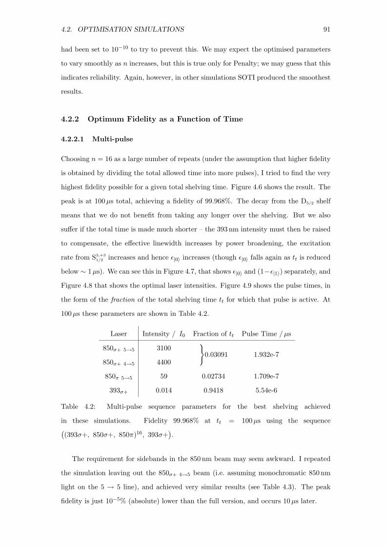
4.2. OPTIMISATION SIMULATIONS 91
had been set to 10−10 to try to prevent this. We may expect the optimised parameters
to vary smoothly as n increases, but this is true only for Penalty; we may guess that this
indicates reliability. Again, however, in other simulations SOTI produced the smoothest
results.
4.2.2 Optimum Fidelity as a Function of Time
4.2.2.1 Multi-pulse
Choosing n = 16 as a large number of repeats (under the assumption that higher fidelity
is obtained by dividing the total allowed time into more pulses), I tried to find the very
highest fidelity possible for a given total shelving time. Figure 4.6 shows the result. The
peak is at 100 µs total, achieving a fidelity of 99.968%. The decay from the D5/2 shelf
means that we do not benefit from taking any longer over the shelving. But we also
suffer if the total time is made much shorter – the 393 nm intensity must then be raised
to compensate, the effective linewidth increases by power broadening, the excitation
rate from S3,+31/2 increases and hence ǫ|0〉 increases (though ǫ|0〉 falls again as tt is reduced
below ∼ 1 µs). We can see this in Figure 4.7, that shows ǫ|0〉 and (1−ǫ|1〉) separately, and
Figure 4.8 that shows the optimal laser intensities. Figure 4.9 shows the pulse times, in
the form of the fraction of the total shelving time tt for which that pulse is active. At
100 µs these parameters are shown in Table 4.2.
Laser Intensity / I0 Fraction of tt Pulse Time / µs
850σ+ 5→5 3100
850σ+ 4→5 4400
0.03091 1.932e-7
850π 5→5 59 0.02734 1.709e-7
393σ+ 0.014 0.9418 5.54e-6
Table 4.2: Multi-pulse sequence parameters for the best shelving achieved
in these simulations. Fidelity 99.968% at tt = 100 µs using the sequence(
(393σ+, 850σ+, 850π)16, 393σ+)
.
The requirement for sidebands in the 850 nm beam may seem awkward. I repeated
the simulation leaving out the 850σ+ 4→5 beam (i.e. assuming monochromatic 850 nm
light on the 5 → 5 line), and achieved very similar results (see Table 4.3). The peak
fidelity is just 10−5% (absolute) lower than the full version, and occurs 10 µs later.

92 CHAPTER 4. READOUT
10−7
10−6
10−5
10−4
10−3
0.9999
0.999
0.99
0.9
0
tt / s
Fid
eli
ty
Maximum
Figure 4.6: Multipulse shelving simulation with n = 16, from stretch states, showing
only the highest fidelity at each value of total time tt.
10−7
10−6
10−5
10−4
10−3
10−4
10−3
10−2
10−1
100
tt / s
1−
P(S
helv
e S
1/2
F=
4)
= ε
|1
>
10−7
10−6
10−5
10−4
10−3
10−4
10−3
10−2
10−1
100
tt / s
P(S
helv
e S
1/2
F=
3)
= ε
|0
>
Figure 4.7: Shelving errors from each qubit state, for the simulations of Figure 4.6.

4.2. OPTIMISATION SIMULATIONS 93
10−14
10−10
10−6
10−2
102
106
1010
85
0σ
+ 5
→5
In
ten
sity
/ I
0
10−14
10−10
10−6
10−2
102
106
1010
85
0σ
+ 4
→5
In
ten
sity
/ I
0
10−7
10−6
10−5
10−4
10−3
10−10
10−6
10−2
102
106
1010
tt / s
85
0π 5
→5
In
ten
sity
/ I
0
10−7
10−6
10−5
10−4
10−3
10−3
10−2
10−1
100
101
102
tt / s
39
3 I
nte
nsi
ty /
I0
Figure 4.8: Optimal intensities for the simulations of Figure 4.6.
0.2
0.3
0.4
0.5
0.6
0.8
1
Fra
c.
of
tt u
sed
for 3
93
10−7
10−6
10−5
10−4
10−3
10−8
10−7
10−6
10−5
10−4
10−3
10−2
10−1
100
tt / s
Fra
c.
of
tt u
sed
for 8
50
σ+
10−7
10−6
10−5
10−4
10−3
10−8
10−7
10−6
10−5
10−4
10−3
10−2
10−1
100
tt / s
Fra
c.
of
tt u
sed
for 8
50
π
Figure 4.9: Optimal pulse times for the simulations of Figure 4.6.
94 CHAPTER 4. READOUT
The parameters plots Figures 4.8 and 4.9 are extremely noisy, demonstrating how
bad the optimiser is. In Figure 4.10 I show the fidelities that the optimiser achieved
when starting with various different guesses – Figure 4.6 is simply the best of these. The
starting guesses are fixed (I do not use the previous best solution as the guess for the
next point) and the found solution jumps as tt increases. This is presumably because
the basin of attraction2 has a complex shape that depends on tt, and thus a starting
guess lies in different basins for different values of tt. For many of the following graphs, I
was able to isolate a particular starting guess that consistently gave the best results for
almost the whole range of times; with the optimal parameter graphs also being smooth.
But this wasn’t true here. One possible reason why this set of simulations was so bad
is that it featured so many parameters: two independent times and four intensities.
Optimisation does become more difficult in higher dimensions. Another idea is that the
fidelity is relatively insensitive to the parameters in this simulation – the optimiser tries
to descend a gradient, and if the function is too flat the optimiser may stop too early.
At very short total times, the shelving is apparently improved by leaving out some
pulses altogether. Each coloured line on Figures 4.11-4.14 shows the optimal fidelities
and parameters for the sequence(
(393σ+, 850σ+, 850π)16, 393σ+)
, with some of the
beams being left out. As well as the result if all beams are allowed, we see(
393σ+)
alone;(
(393σ+, 850π)16, 393σ+)
; and(
(393σ+, 850σ+)16, 393σ+)
. Notice how 393σ+ alone
is best at times < 0.6 µs; 393 and 850π are best in the range 0.6 µs < tt < 1.4 µs; and
using all the beams is best for tt > 1.4 µs. The naıve explanation is that, at short times,
maximising t393 (and thus allowing the 393 intensity to be reduced) yields a greater
fidelity than using some of the time to repump from D3/2. However, we also find this
effect when shelving with a single pulse, so this might not be the correct explanation.
Another reason is suggested below.
It is not necessarily best to use n = 16 repeats. In Figures 4.15-4.18 I show the
optimal results achieved for n = 16, 8, 4, 2 and 1. We see that, while large n gives the
best fidelity overall, for short total times it is better to have a smaller number of repeats.
2When trying to find the roots (or extrema) of a function, using some iterative numerical method, the
basin of attraction of root xi is the set of starting guesses x0,i such that the successive approximations
x0,i, x1,i, x2,i, . . . converge to xi. Many beautiful fractals are based on basins of attraction for, for
instance, Newton’s method of root finding. See, for instance, Gleick [? ] or almost any other book about
chaos and fractals.
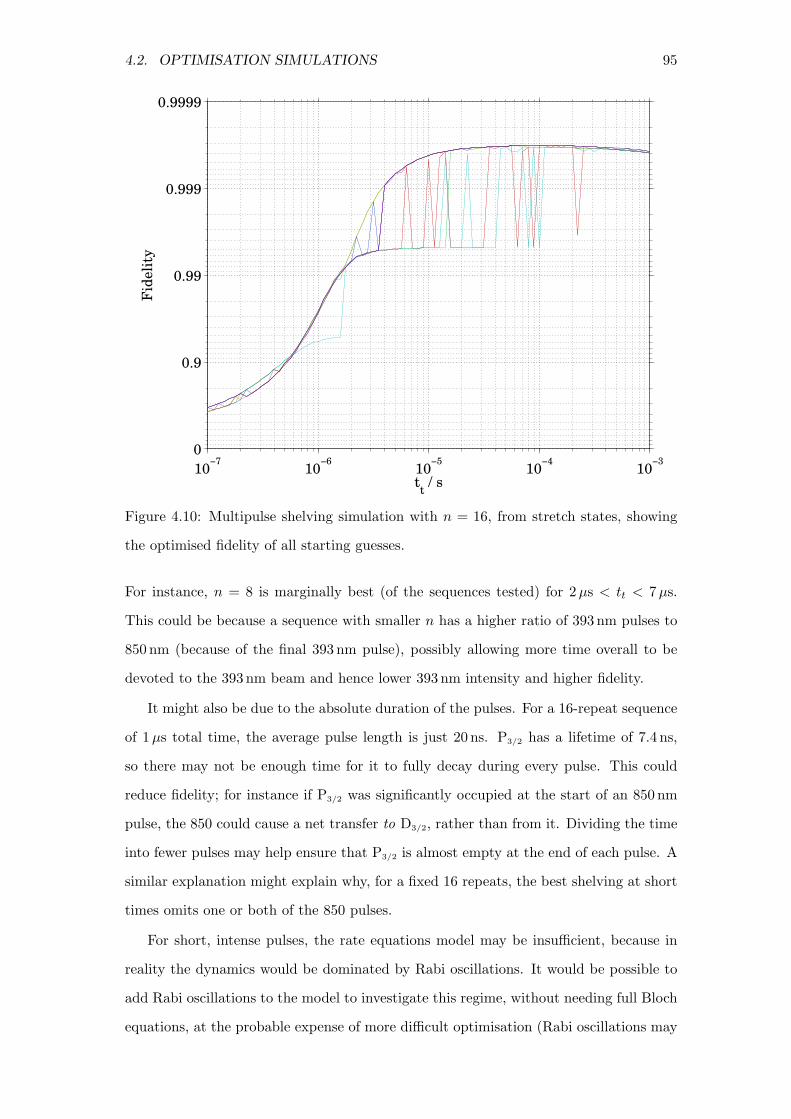
4.2. OPTIMISATION SIMULATIONS 95
10−7
10−6
10−5
10−4
10−3
0.9999
0.999
0.99
0.9
0
tt / s
Fid
eli
ty
Figure 4.10: Multipulse shelving simulation with n = 16, from stretch states, showing
the optimised fidelity of all starting guesses.
For instance, n = 8 is marginally best (of the sequences tested) for 2 µs < tt < 7 µs.
This could be because a sequence with smaller n has a higher ratio of 393 nm pulses to
850 nm (because of the final 393 nm pulse), possibly allowing more time overall to be
devoted to the 393 nm beam and hence lower 393 nm intensity and higher fidelity.
It might also be due to the absolute duration of the pulses. For a 16-repeat sequence
of 1 µs total time, the average pulse length is just 20 ns. P3/2 has a lifetime of 7.4 ns,
so there may not be enough time for it to fully decay during every pulse. This could
reduce fidelity; for instance if P3/2 was significantly occupied at the start of an 850 nm
pulse, the 850 could cause a net transfer to D3/2, rather than from it. Dividing the time
into fewer pulses may help ensure that P3/2 is almost empty at the end of each pulse. A
similar explanation might explain why, for a fixed 16 repeats, the best shelving at short
times omits one or both of the 850 pulses.
For short, intense pulses, the rate equations model may be insufficient, because in
reality the dynamics would be dominated by Rabi oscillations. It would be possible to
add Rabi oscillations to the model to investigate this regime, without needing full Bloch
equations, at the probable expense of more difficult optimisation (Rabi oscillations may

96 CHAPTER 4. READOUT
10−7
10−6
10−5
10−4
10−3
0.9999
0.999
0.99
0.9
0
tt / s
Fid
eli
ty
393, 850π and 850σ+
393 only
393 and 850π only
393 and 850σ+ only
Best
Figure 4.11: Multipulse shelving simulation with n = 16, from stretch states, showing
optimised shelving fidelity.
10−7
10−6
10−5
10−4
10−3
10−4
10−3
10−2
10−1
100
tt / s
1−
P(S
helv
e S
1/2
F=
4)
= ε
|1
>
10−7
10−6
10−5
10−4
10−3
10−4
10−3
10−2
10−1
100
tt / s
P(S
helv
e S
1/2
F=
3)
= ε
|0
>
Figure 4.12: Shelving errors from each qubit state, for the simulations of Figure 4.11.
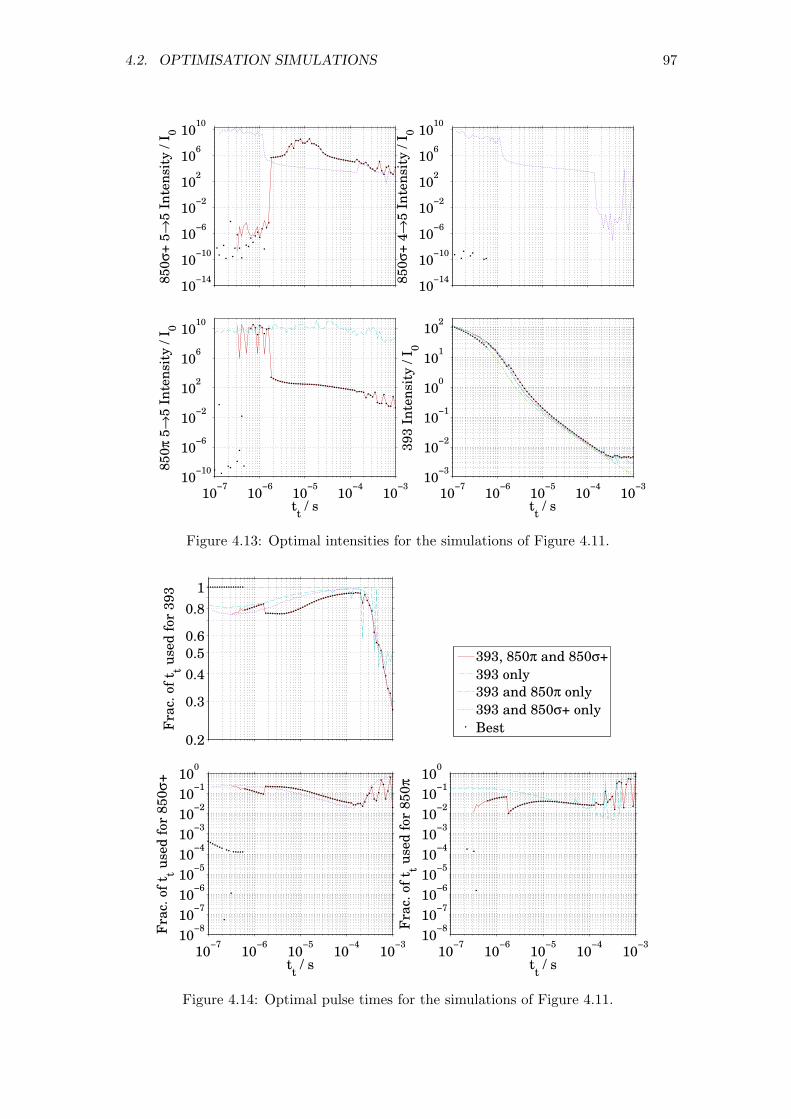
4.2. OPTIMISATION SIMULATIONS 97
10−14
10−10
10−6
10−2
102
106
1010
85
0σ
+ 5
→5
In
ten
sity
/ I
0
10−14
10−10
10−6
10−2
102
106
1010
85
0σ
+ 4
→5
In
ten
sity
/ I
0
10−7
10−6
10−5
10−4
10−3
10−10
10−6
10−2
102
106
1010
tt / s
85
0π 5
→5
In
ten
sity
/ I
0
10−7
10−6
10−5
10−4
10−3
10−3
10−2
10−1
100
101
102
tt / s
39
3 I
nte
nsi
ty /
I0
Figure 4.13: Optimal intensities for the simulations of Figure 4.11.
393, 850π and 850σ+
393 only
393 and 850π only
393 and 850σ+ only
Best0.2
0.3
0.4
0.5
0.6
0.8
1
Fra
c. o
f t t u
sed
for
39
3
10−7
10−6
10−5
10−4
10−3
10−8
10−7
10−6
10−5
10−4
10−3
10−2
10−1
100
tt / s
Fra
c. o
f t t u
sed
for
85
0σ
+
10−7
10−6
10−5
10−4
10−3
10−8
10−7
10−6
10−5
10−4
10−3
10−2
10−1
100
tt / s
Fra
c. o
f t t u
sed
for
85
0π
Figure 4.14: Optimal pulse times for the simulations of Figure 4.11.

98 CHAPTER 4. READOUT
lead to numerous local minima).
4.2.2.2 Single Pulse, Multiple 850 nm Beams
For the single pulse shelving method, I first assumed exactly the same laser situation
as in the previous section (three 850 nm beams, each with its intensity independently
optimised). But all four beams are switched on together during a pulse of length tt.
Figures 4.19-4.21 show the results.
We see that although the overall best fidelity is very slightly lower than for multipulse
shelving (99.965% rather than 99.968%) the biggest difference is that the fidelity takes
more than twice as long to reach the 99.9% level (8.4 µs rather than 3.5 µs). This could
be because the 850π beam is on while there is still significant population in D(4,5),+4
3/2 ,
exciting some population to P3/2 states that are not P5,+53/2 , whence it can ultimately fall
back to |0〉 and be lost. The optimiser has to choose the 850π intensity to compromise
between that process, and leaving population in D5,+53/2 ; while in the pulsed method the
intensity can be made much stronger.
Figures 4.8 and 4.21 show that all the 850 beams are stronger in the pulsed method
than in the single pulse method. Remember that very high-intensity 850 beams equalise
the populations of P3/2 and D3/2, and so could reduce the population of P3/2 and hence
the shelving rate. This might also explain why, at short times, it is best to leave some
of the 850 beams off altogether.
4.2.2.3 Single Pulse, Single 850 nm Beam
Here I simulate another single-pulse shelving method (850 and 393 on at the same time).
This time I use a single, monochromatic, circularly polarised 850 nm beam at angle θ
to the magnetic field direction – this is the situation in our experiment as described in
Section 4.1.2. Our experiment has θ = 2.3(1). For the simulation I take a range of
angles, starting at 90 and halving each time: 90, 45, 22.5, 11.25, 5.625, 2.8125,
1.40625, 0.703125 and 0.3515625. However, I used 2.3 rather than 2.8125 for better
comparison with the experiment. Optimisation is relatively easy now because there are
only three quantities to optimise: the 393 nm and 850 nm intensities, and the frequency
of the 850 nm beam. I optimised the frequency manually, running the optimisation
repeatedly while scanning the frequency and taking more closely-spaced points where
the results looked good. The automatic optimiser might have found only local optima.

4.2. OPTIMISATION SIMULATIONS 99
10−7
10−6
10−5
10−4
10−3
0.9999
0.999
0.99
0.9
0
tt / s
Fid
eli
ty
16
8
4
2
1
n =
Figure 4.15: Multipulse shelving simulation with various n, from stretch states, showing
optimised shelving fidelity.
10−7
10−6
10−5
10−4
10−3
10−4
10−3
10−2
10−1
100
tt / s
1−
P(S
helv
e S
1/2
F=
4)
= ε
|1
>
10−7
10−6
10−5
10−4
10−3
10−4
10−3
10−2
10−1
100
tt / s
P(S
helv
e S
1/2
F=
3)
= ε
|0
>
Figure 4.16: Shelving errors from each qubit state, for the simulations of Figure 4.15.
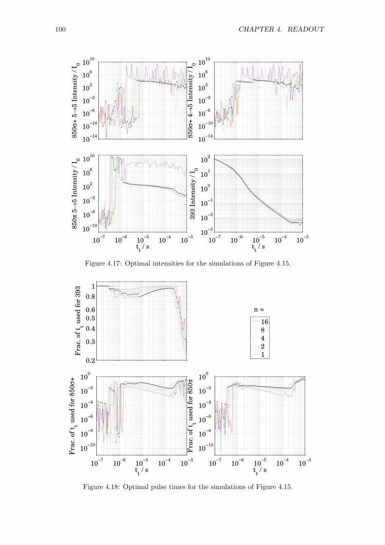
100 CHAPTER 4. READOUT
10−14
10−10
10−6
10−2
102
106
1010
85
0σ
+ 5
→5
In
ten
sity
/ I
0
10−14
10−10
10−6
10−2
102
106
1010
85
0σ
+ 4
→5
In
ten
sity
/ I
0
10−7
10−6
10−5
10−4
10−3
10−10
10−6
10−2
102
106
1010
tt / s
85
0π 5
→5
In
ten
sity
/ I
0
10−7
10−6
10−5
10−4
10−3
10−3
10−2
10−1
100
101
102
tt / s
39
3 I
nte
nsi
ty /
I0
Figure 4.17: Optimal intensities for the simulations of Figure 4.15.
16
8
4
2
1
n =
0.2
0.3
0.4
0.5
0.6
0.8
1
Fra
c.
of
tt u
sed
for 3
93
10−7
10−6
10−5
10−4
10−3
10−10
10−8
10−6
10−4
10−2
100
tt / s
Fra
c.
of
tt u
sed
for 8
50
σ+
10−7
10−6
10−5
10−4
10−3
10−10
10−8
10−6
10−4
10−2
100
tt / s
Fra
c.
of
tt u
sed
for 8
50
π
Figure 4.18: Optimal pulse times for the simulations of Figure 4.15.

4.2. OPTIMISATION SIMULATIONS 101
10−7
10−6
10−5
10−4
10−3
0.9999
0.999
0.99
0.9
0
tt / s
Fid
eli
ty
393, 850π and 850σ+
393 only
393 and 850π only
393 and 850σ+ only
Figure 4.19: Single pulse shelving simulation, from stretch states, showing optimised
shelving fidelity.
Figures 4.22-4.25 show the frequency scan for every second 850 angle. The frequen-
cies of the hyperfine components of the 850 nm transition have also been marked on,
and labeled with the notation: DF=?3/2 → PF=?
3/2 . (note this is the opposite direction to
the notation of Appendix A). Each coloured line shows the scan for a particular total
shelving time. The optimal frequency for each time is marked with a filled symbol. A
few scans had their maxima at detunings well outside the range shown; they can be seen
in Figure 4.28.
We see an interesting trend. At θ = 90 (the polarisation ratio at the ion is Iπ : Iσ+ :
Iσ− = 12 : 1
4 : 14), the best shelving occurs near the D4
3/2 → P53/2 component, and the
worst is near D53/2 → P4
3/2 (except at the shortest times). At 22.5 we see deep valleys at
D43/2 → P4
3/2, D43/2 → P3
3/2 and D53/2 → P4
3/2. As the angle narrows further, and the beam
becomes more purely σ+ polarised at the ion, the D53/2 → P5
3/2 component becomes more
and more favourable. Below 1.406 there is little further change.
The last observation is easiest to explain: the π component of the light becomes
weaker as θ falls, so to effectively repump from D5,+53/2 the beam must be tuned more
closely to D53/2 → P5
3/2. As θ becomes larger the π component becomes stronger and
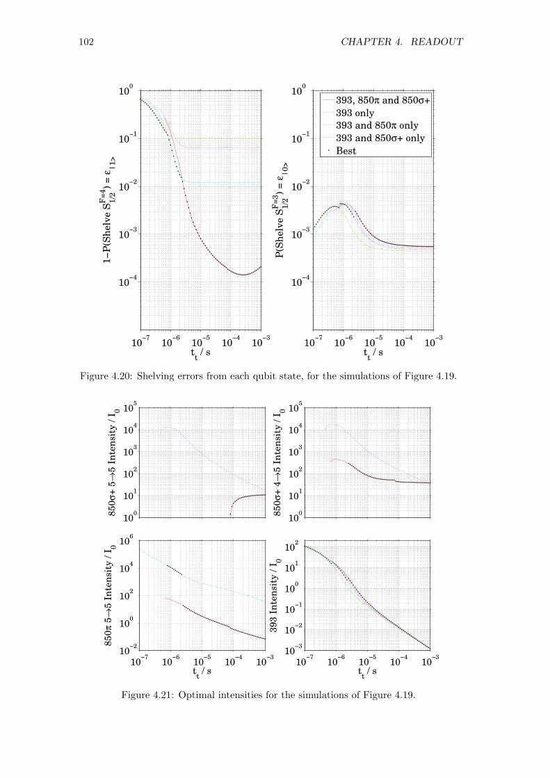
102 CHAPTER 4. READOUT
10−7
10−6
10−5
10−4
10−3
10−4
10−3
10−2
10−1
100
tt / s
1−
P(S
helv
e S
1/2
F=
4)
= ε
|1
>
10−7
10−6
10−5
10−4
10−3
10−4
10−3
10−2
10−1
100
tt / s
P(S
helv
e S
1/2
F=
3)
= ε
|0
>
393, 850π and 850σ+
393 only
393 and 850π only
393 and 850σ+ only
Best
Figure 4.20: Shelving errors from each qubit state, for the simulations of Figure 4.19.
100
101
102
103
104
105
85
0σ
+ 5
→5
In
ten
sity
/ I
0
100
101
102
103
104
105
85
0σ
+ 4
→5
In
ten
sity
/ I
0
10−7
10−6
10−5
10−4
10−3
10−2
100
102
104
106
tt / s
85
0π 5
→5
In
ten
sity
/ I
0
10−7
10−6
10−5
10−4
10−3
10−3
10−2
10−1
100
101
102
tt / s
39
3 I
nte
nsi
ty /
I0
Figure 4.21: Optimal intensities for the simulations of Figure 4.19.
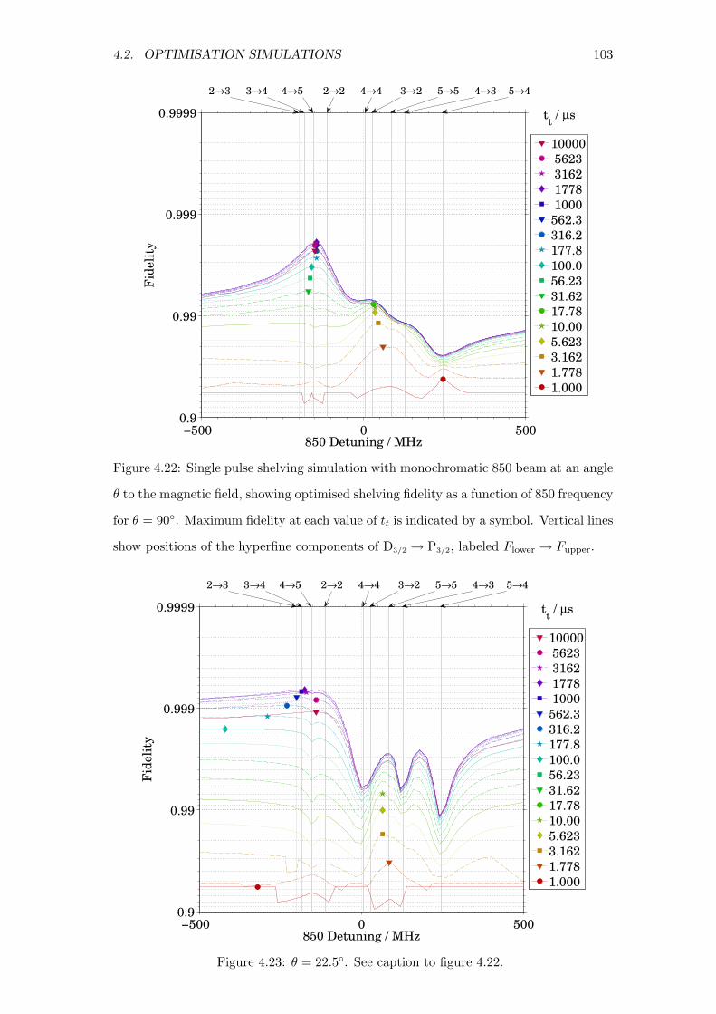
4.2. OPTIMISATION SIMULATIONS 103
−500 0 500
0.9999
0.999
0.99
0.9
850 Detuning / MHz
Fid
eli
ty
10000
5623
3162
1778
1000
562.3
316.2
177.8
100.0
56.23
31.62
17.78
10.00
5.623
3.162
1.778
1.000
tt / µs
2→3 3→4 4→5 2→2 4→4 3→2 5→5 4→3 5→4
Figure 4.22: Single pulse shelving simulation with monochromatic 850 beam at an angle
θ to the magnetic field, showing optimised shelving fidelity as a function of 850 frequency
for θ = 90. Maximum fidelity at each value of tt is indicated by a symbol. Vertical lines
show positions of the hyperfine components of D3/2 → P3/2, labeled Flower → Fupper.
−500 0 500
0.9999
0.999
0.99
0.9
850 Detuning / MHz
Fid
eli
ty
10000
5623
3162
1778
1000
562.3
316.2
177.8
100.0
56.23
31.62
17.78
10.00
5.623
3.162
1.778
1.000
tt / µs
2→3 3→4 4→5 2→2 4→4 3→2 5→5 4→3 5→4
Figure 4.23: θ = 22.5. See caption to figure 4.22.

104 CHAPTER 4. READOUT
−500 0 500
0.9999
0.999
0.99
0.9
850 Detuning / MHz
Fid
eli
ty
10000
5623
3162
1778
1000
562.3
316.2
177.8
100.0
56.23
31.62
17.78
10.00
5.623
3.162
1.778
1.000
tt / µs
2→3 3→4 4→5 2→2 4→4 3→2 5→5 4→3 5→4
Figure 4.24: θ = 5.625. See caption to figure 4.22.
−500 0 500
0.9999
0.999
0.99
0.9
850 Detuning / MHz
Fid
eli
ty
10000
5623
3162
1778
1000
562.3
316.2
177.8
100.0
56.23
31.62
17.78
10.00
5.623
3.162
1.778
1.000
tt / µs
2→3 3→4 4→5 2→2 4→4 3→2 5→5 4→3 5→4
Figure 4.25: θ = 1.40625. See caption to figure 4.22.

4.2. OPTIMISATION SIMULATIONS 105
accurate tuning becomes unnecessary, and the σ− component is also becoming stronger.
D43/2 → P3
3/2 and D53/2 → P4
3/2 have strong σ− components from D4,+43/2 and D5,(+4,+5)
3/2 which
the 850 beam had best avoid, else the shelving process loses its selection-rule protection
from falling back to |0〉. Similarly D43/2 → P4
3/2 has a strong π component from D4,+43/2 that
should be avoided. This explains the valleys in the 22.5 plot. It is not clear why the
D43/2 → P5
3/2 transition is favoured for θ = 90, but becomes a valley at smaller angles.
The overall optimised fidelities, shelving errors and parameters are shown in Figures
4.26-4.28. At 2.3 we should be able to shelve at 99.962% fidelity in 300 µs, at an entirely
reasonable 850 intensity of 190 I0 (the optimal 393 intensity is 0.004 I0). By chance, our
experimental beam is close to the optimal angle. For smaller angles, shelving becomes
much slower (limited by the low power in the π component). Notice that there are places
where the optimal 850 detuning (and 850 intensity) become extremely large; however
the best shelving at a given angle always occurs at such a time that it avoids those
anomalies.
10−6
10−5
10−4
10−3
10−2
0.9999
0.999
0.99
0.9
tt / s
Fid
eli
ty
0.352
0.703
1.406
2.3
5.625
11.25
22.5
45
90
850 Angle
/ Degrees
Figure 4.26: Single pulse shelving simulation with monochromatic 850 beam at an angle
θ to the magnetic field, showing optimised shelving fidelity.

106 CHAPTER 4. READOUT
10−6
10−5
10−4
10−3
10−2
10−4
10−3
10−2
10−1
100
tt / s
1−
P(S
helv
e S
1/2
F=
4)
= ε
|1
>
10−6
10−5
10−4
10−3
10−2
10−4
10−3
10−2
10−1
100
tt / s
P(S
helv
e S
1/2
F=
3)
= ε
|0
>
Figure 4.27: Shelving errors from each qubit state, for the simulations of Figure 4.26.
100
101
102
103
104
105
106
107
85
0 I
nte
nsi
ty /
I0
10−6
10−5
10−4
10−3
10−2
10−4
10−3
10−2
10−1
100
101
Total Time / s
39
3 I
nte
nsi
ty /
I0
10−6
10−5
10−4
10−3
10−2
−2000
−1500
−1000
−500
0
500
tt / s
85
0 D
etu
nin
g /
MH
z
0.352
0.703
1.406
2.3
5.625
11.25
22.5
45
90
850 Angle /
Degrees
Figure 4.28: Optimal intensities and 850 frequency for the simulations of Figure 4.26.

4.2. OPTIMISATION SIMULATIONS 107
4.2.2.4 Clock States
Future experiments with 43Ca+ will mostly use the MF = 0 clock states, because they
have a much lower susceptibility to magnetic field fluctuations than stretched states.
When using our shelving procedure from S4,01/2, we can no longer rely on using the ap-
proximate cycling transitions through P5,+53/2 , so we lose much of the protection against
decays to |0〉. There is some protection due to the 160 MHz hyperfine splitting between
P53/2 and P4
3/2: the 393 nm beam is tuned to excite to P53/2, and selection rules then
forbid a direct decay to S31/2. Figures 4.29-4.32 and 4.33-4.35 are the equivalents of
Figures 4.11-4.14 and 4.19-4.21 for shelving from a clock state qubit. The 16-pulse and
single-pulse methods both reach a fidelity of 99.64% – an error that is ten times that
for shelving from stretch states. This is almost entirely due to a rise in ǫ|1〉 rather than
ǫ|0〉, because unwanted decays to |0〉 are more likely than with stretch-state shelving.
There might be possible improvements – perhaps allowing extra beams with the
polarisations I have so far ignored. But in practice, it might be better to use four
microwave or Raman pulses to coherently transfer from clock state to stretch state; S4,01/2
to S4,+41/2 [128, Section III.C.2-3]. This becomes worthwhile if the transfer pulses each
have average error 8 × 10⁻⁴. General fault tolerance demands single-qubit gates with
errors of order 10−3 or better, and the same technology could almost certainly perform
this function too. However these transfer pulses would not be insensitive to magnetic
field fluctuations, and so would be more prone to error than operations between the
clock states.
4.2.2.5 Summary
Figure 4.36 compares the multipulse, single-pulse and 850-at-angle methods, summaris-
ing Figures 4.15, 4.19 and 4.26. Table 4.3 collects together some of the best optimised
results from this section.
4.2.3 Fidelity as a Function of Parameters
It is important to consider how the shelving fidelity is affected by perturbations in the
sequence. I have chosen the best of all the preceding simulations as an example, because
the perturbations should have a greater relative effect at higher fidelities. As a reminder,
this is the pulse sequence(
(393σ+, 850σ+, 850π)16, 393σ+)
, that achieved a fidelity

108 CHAPTER 4. READOUT
10−7
10−6
10−5
10−4
10−3
0.999
0.99
0.9
0
tt / s
Fid
eli
ty
393, 850π and 850σ+
393 only
393 and 850π only
393 and 850σ+ only
Figure 4.29: Multipulse shelving simulation with n = 16, from clock states (S4,01/2 and
S3,01/2), showing optimised shelving fidelity.
10−7
10−6
10−5
10−4
10−3
10−4
10−3
10−2
10−1
100
tt / s
1−
P(S
helv
e S
1/2
F=
4)
= ε
|1
>
10−7
10−6
10−5
10−4
10−3
10−4
10−3
10−2
10−1
100
tt / s
P(S
helv
e S
1/2
F=
3)
= ε
|0
>
Figure 4.30: Shelving errors from each qubit state, for the simulations of Figure 4.29.
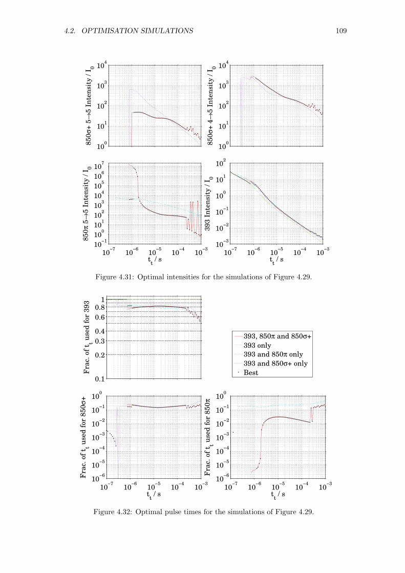
4.2. OPTIMISATION SIMULATIONS 109
100
101
102
103
104
85
0σ
+ 5
→5
In
ten
sity
/ I
0
100
101
102
103
104
85
0σ
+ 4
→5
In
ten
sity
/ I
0
10−7
10−6
10−5
10−4
10−3
10−1
100
101
102
103
104
105
106
107
tt / s
85
0π 5
→5
In
ten
sity
/ I
0
10−7
10−6
10−5
10−4
10−3
10−3
10−2
10−1
100
101
102
tt / s
39
3 I
nte
nsi
ty /
I0
Figure 4.31: Optimal intensities for the simulations of Figure 4.29.
393, 850π and 850σ+
393 only
393 and 850π only
393 and 850σ+ only
Best0.1
0.2
0.3
0.4
0.6
0.81
Fra
c. o
f t t u
sed
for
39
3
10−7
10−6
10−5
10−4
10−3
10−6
10−5
10−4
10−3
10−2
10−1
100
tt / s
Fra
c. o
f t t u
sed
for
85
0σ
+
10−7
10−6
10−5
10−4
10−3
10−6
10−5
10−4
10−3
10−2
10−1
100
tt / s
Fra
c. o
f t t u
sed
for
85
0π
Figure 4.32: Optimal pulse times for the simulations of Figure 4.29.

110 CHAPTER 4. READOUT
10−7
10−6
10−5
10−4
10−3
0.999
0.99
0.9
0
tt / s
Fid
eli
ty
393, 850π and 850σ+
393 only
393 and 850π only
393 and 850σ+ only
Figure 4.33: Single pulse shelving simulation, from clock states, showing optimised
shelving fidelity.
of 99.968% in 100 µs. Details were in Table 4.2.
First I look at intensity error. Keeping all other aspects of the simulation constant,
one of the beams in the sequence had its intensity scanned. The fidelity achieved as
a function of the intensity is shown in Figure 4.37. The intensity axis is shown as a
multiplier of the optimal intensity, so that x = 1 represents the optimal sequence for all
the lines. We see that shelving is highly insensitive to the 850 intensities – except for
having the 850π too weak, the intensities can be orders of magnitude different with very
little effect. The 393 intensity is (as expected) much more sensitive; but even so, it can
be a factor of three overpowered (or 40% underpowered) and still exceed 99.9% fidelity.
Next, I consider errors in the pulse times. Figure 4.38 shows the shelving fidelity as
a function of the fraction of the total time dedicated to a particular pulse. For instance,
at x = 0.6 the red 393 curve shows the result when the seventeen 393 pulses together
filled 60% of the total shelving time – the other 40% was divided among 850σ+ and 850π
in the same ratio as in the optimal sequence (1.13 : 1, shown as a diamond marker). As
in the previous graph, the shelving is resilient to changing the 850 pulses – as long as
neither pulse makes up less than ∼ 20% of the total 850 allowance, the fidelity is very

4.2. OPTIMISATION SIMULATIONS 111
10−7
10−6
10−5
10−4
10−3
10−4
10−3
10−2
10−1
100
tt / s
1−
P(S
helv
e S
1/2
F=
4)
= ε
|1
>
10−7
10−6
10−5
10−4
10−3
10−4
10−3
10−2
10−1
100
tt / s
P(S
helv
e S
1/2
F=
3)
= ε
|0
>
393, 850π and 850σ+
393 only
393 and 850π only
393 and 850σ+ only
Best
Figure 4.34: Shelving errors from each qubit state, for the simulations of Figure 4.33.
10−1
100
101
102
85
0σ
+ 5
→5
In
ten
sity
/ I
0
10−1
100
101
102
85
0σ
+ 4
→5
In
ten
sity
/ I
0
10−7
10−6
10−5
10−4
10−3
10−2
10−1
100
101
102
103
tt / s
85
0π 5
→5
In
ten
sity
/ I
0
10−7
10−6
10−5
10−4
10−3
10−3
10−2
10−1
100
101
102
tt / s
39
3 I
nte
nsi
ty /
I0
Figure 4.35: Optimal intensities for the simulations of Figure 4.33.

112 CHAPTER 4. READOUT
10−7
10−6
10−5
10−4
10−3
0.9999
0.999
0.99
0.9
0
tt / s
Fid
eli
ty
Multipulse (any n)
Single pulse, multiple 850
Single pulse, 850 at angle
Figure 4.36: The best fidelities available for shelving from stretch states, for the three
major methods discussed in this section, as a function of total shelving time. For
multipulse, the maximum over the number n of repeats has been taken; for 850-at-
angle, the maximum over all angles has been taken.
Method Qubit Optimal Optimal ǫ at
ǫ tt / µs tt = 10 µs
Multipulse (n = 16) Stretch 3.21 × 10⁻⁴ 100 4.16 × 10⁻⁴
n = 16, without 850σ+ 4→5 Stretch 3.21 × 10⁻⁴ 110 4.18 × 10⁻⁴
Single pulse, multiple 850 Stretch 3.50 × 10⁻⁴ 300 8.60 × 10⁻⁴
Single pulse, 850 at angle Stretch 3.68 × 10⁻⁴ 300 1.60 × 10⁻³
Multipulse (n = 16) Clock 3.57 × 10⁻³ 200 4.03 × 10⁻³
Single pulse, multiple 850 Clock 3.64 × 10⁻³ 600 5.32 × 10⁻³
Table 4.3: Summary of the best optimised shelving simulations from Section 4.2.2. The
very lowest error achieved with each method is listed, along with the total shelving time
required. I also state the error that can be reached with just 10 µs shelving (the time
that Steane allows for readout in [134]).

4.2. OPTIMISATION SIMULATIONS 113
10−4
10−3
10−2
10−1
100
101
102
103
104
0.9999
0.999
0.99
0.9
0
Intensity Multiplier
Fid
eli
ty
393
850σ+ 5→5
850σ+ 4→5
850π 5→5
Changed Beam
Figure 4.37: Multipulse shelving simulation with n = 16, from stretch states, varying
the intensities from the optimum.
near its optimum. Again, the 393 pulse is much more sensitive, but not too much. As
long as the 393 is on for between 62% and 99.6% of the sequence, the fidelity is at least
99.9%. The 393 pulses are each 5.5 µs long; a 0.1 µs timing error would increase the
shelving error by only 10−6 absolute.
Figure 4.39 shows the effect of detuning the lasers from resonance (recall that the 393
is tuned to S41/2 → P5
3/2, and the 850 has components at D53/2 → P5
3/2 and D43/2 → P5
3/2).
As may be expected, the 393 is most frequency-sensitive, but an error of & 2 MHz is
needed to significantly reduce the fidelity.
I calculated the effect of polarisation impurity in the laser beams, in Figure 4.40. I
have assumed in every case that the impurity appears as σ− polarised light (I did not
simulate, for instance, a mis-set waveplate), with an intensity that makes up the stated
fraction of the relevant beam. The correctly polarised intensity is reduced to match,
so that at a polarisation impurity of 1 the relevant beam is entirely σ− polarised. For
the 850σ+ beam, I assume both frequency components are affected to the same extent.
This time the 850σ+ is the most sensitive beam, and 850π the least. Notice that even
in the worst of these cases, a pure σ− 393 beam, the fidelity is still above 94%.

114 CHAPTER 4. READOUT
0 0.1 0.2 0.3 0.4 0.5 0.6 0.7 0.8 0.9 1
0.9999
0.999
0.99
0.9
0
Pulse Time Fraction
Fid
eli
ty
t393
/ (t393
+t850σ+
+t850π
) [Marker indicates optimum]
t850σ+
/ (t850σ+
+t850π
) [Marker indicates optimum]
Figure 4.38: Multipulse shelving simulation, from stretch states, varying the pulse times
from the optimum.
100
101
102
103
0.9999
0.999
0.99
0.9
0
Frequency Error / MHz
Fid
eli
ty
393
850σ+ 5→5
850σ+ 4→5
850π 5→5
Changed Beam
Figure 4.39: Multipulse shelving simulation, from stretch states, varying the laser fre-
quencies.

4.2. OPTIMISATION SIMULATIONS 115
10−5
10−4
10−3
10−2
10−1
100
0.9999
0.999
0.99
0.9
Polarisation Impurity
Fid
eli
ty
393
850σ+
850π
σ− Impurity in
Figure 4.40: Multipulse shelving simulation, from stretch states, varying the polarisation
impurities of the beams.
Finally, the simulations were repeated for the best single shelving pulse (the peak
of Figure 4.19). Figures 4.41-4.43 show a similar robustness to the multipulse method;
with the exceptions that this time the fidelity is significantly harmed by having too much
850 power, and the single-pulse method is less sensitive to 850σ+ polarisation impurity.

116 CHAPTER 4. READOUT
10−4
10−3
10−2
10−1
100
101
102
103
104
0.9999
0.999
0.99
0.9
0
Intensity Multiplier
Fid
eli
ty
393
850σ+ 5→5
850σ+ 4→5
850π 5→5
Changed Beam
Figure 4.41: Single pulse shelving simulation, from stretch states, varying the intensities
from the optimum.
100
101
102
103
0.9999
0.999
0.99
0.9
0
Frequency Error / MHz
Fid
eli
ty
393
850σ+ 5→5
850σ+ 4→5
850π 5→5
Changed Beam
Figure 4.42: Single pulse shelving simulation, from stretch states, varying the laser
frequencies.
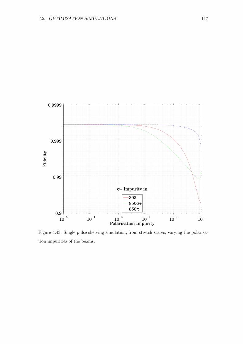
4.2. OPTIMISATION SIMULATIONS 117
10−5
10−4
10−3
10−2
10−1
100
0.9999
0.999
0.99
0.9
Polarisation Impurity
Fid
eli
ty
393
850σ+
850π
σ− Impurity in
Figure 4.43: Single pulse shelving simulation, from stretch states, varying the polarisa-
tion impurities of the beams.

118 CHAPTER 4. READOUT
4.3 Experiments
4.3.1 850 nm Parallel to Magnetic Field
In an early experiment, the sequence (393, 850, 393, 850, 393) was implemented, on
an ion prepared in S4,+41/2 . The 393 nm pulse time was 100 µs; the 850 nm pulse time
was scanned. This time, the magnetic field had been aligned along the 850 nm beam
direction, so the 850 nm π component was very weak. The results, and a simulation
of them, are shown in Figure 4.44. The simulation fits the data only if ∼ 2% of the
850 nm beam is set to be σ− polarised; also the simulation assumes 1% initialisation
error (prepared in S3,+31/2 ). This initialisation error also includes fluorescence-detection
errors. The best seven data points (t850 ≥ 300 µs) have an average of 97.7(2)% shelving.
Notice that, as the polarisation impurity of the 850 nm beam increases, the shelving
becomes much faster for only a small decrease in shelving. But it is only a small decrease
compared to the large overall shelving error. [Speed-up???]
10−6
10−5
10−4
10−3
0.9
0.91
0.92
0.93
0.94
0.95
0.96
0.97
0.98
0.99
Time of each 850 nm Pulse / s
Pro
ba
bil
ity o
f D
ete
ctin
g I
on
as
Sh
elv
ed
50% σ− in 850
4% σ− in 850
2% σ− in 850
1% σ− in 850
Figure 4.44: Experiment (black points) and simulation of shelving sequence (393, 850,
393, 850, 393). I393 = 0.0097 I0, I850 = 2680 I0. Simulation assumes 1% preparation
impurity. Error bars on the experimental data points are statistical only.

4.3. EXPERIMENTS 119
4.3.2 850 nm at Small Angle to Magnetic Field
In an attempt to improve the state preparation, we realigned the magnetic field along
the 397 nm σ beam (improving the purity of σ+ light at the ion). Since the 850 nm
beam was now at a small angle to the magnetic field, we discovered that it excited
π transitions at the ion strongly enough to effectively reclaim from D5,+53/2 – even after
we added a second polarising-beam-splitter (PBS) to the 850 nm beam to improve its
polarisation purity.
4.3.2.1 Various Results
The major aim of the experiments was to achieve the best possible fidelity, rather than to
test rate equations theory. So we made many trials individually, with various parameters
altered, rather than a series of experiments varying only one parameter at a time. The
only feasible way to present such results is as a table, and so Table 4.4 shows a selection of
results from our final set of experiments. In the next few sections I will select particular
rows from the table and explain their significance
Explanation of fields:
Row: An index number for reference.
Date: The date is in DDMMYY format.
File: Usually the data file is “CA43.xxx” where xxx is this number.
Fidelity, ǫ|0〉and 1 − ǫ|1〉: These are the fidelities and error probabilities as deduced by
detecting fluorescence. Photon counting may give an erroneous reading even if the
shelving were perfect, and no attempt is made here to subtract this contribution
to the infidelity; typically the contribution is 0.1% infidelity.
S4,+41/2 Preparation: As described below, the fidelity of population preparation depends
on the frequency of the 397 nm σ beam. This column shows whether the carrier
frequency of this beam was tuned to S41/2 → P4
1/2 or S31/2 → P4
1/2 (the sideband
excites out of the other hyperfine level of S1/2 in both cases). For 3 → 4, the usual
optical pumping pulse can be followed by a pulse with this same beam, with the
EOM switched off, which should improve the preparation as discussed below.
t393 and t850: For multipulse sequences, these are the times per pulse. For single-pulse
experiments, the time of the combined 393/850 pulse is given as t393.

120 CHAPTER 4. READOUT
I393 and I850: On 290507, a microscope slide pickoff (that reflected some light for
spot-size and beam-power measurement) was removed from the σ beams’ paths,
to improve polarisation purity. From this point on, the listed intensities are less
reliable because the beam powers were measured by different sensors.
Sequence: If the entry is a number, that number is n representing the shelving pulse se-
quence(
(393 nm, 850 nm)n, 393 nm)
; “Single” refers to a single pulse during which
both the 393 nm and 850 nm lasers were switched on.
854 nm Shutter: When the shutter was not used (“N”), the 854 was switched off only
using its AOM; leakage through the AOM could contribute to ǫ|1〉 by deshelving
the ion. When the shutter was used (“Y”), the laser was blocked completely during
the shelving and fluorescence detection phases.
4.3.2.2 Population-Preparation Improvement
For the early experiment of Figure 4.44, the 397 nm laser had its carrier tuned to
S41/2 → P4
1/2, the sideband to S31/2 → P4
1/2. This allowed S31/2 to be prepared simply
by turning the EOM off. But we discovered that the population preparation was im-
proved by exchanging the frequencies of carrier and sideband. The carrier is the more
intense component, so the new tuning increased excitation from S31/2 and so reduced its
population. Also, the impact of any polarisation impurity (exciting out of the desired
state P4,+41/2 ) is reduced. This configuration also allowed us to turn the EOM off briefly
at the end of state preparation, to pump any remaining population from S31/2 to S4
1/2.
We performed an experiment that measured the rate at which the 397 nm σ beam
pumped out of S4,+41/2 . Together with simulations, I deduce that the nominally σ+ beam
contains 0.9(2)% σ− impurity (assuming all the depumping is due to this beam; in
fact there is also a large contribution from the 397 nm Doppler beam leaking through
its AOM, but the particular source of the impurity is irrelevant for these purposes).
This improved from an earlier figure of 1.86(11)% before the pickoff was removed. If
the carrier were tuned to S41/2 → P4
1/2, 0.9% polarisation impurity in the beam would
prepare S4,+41/2 just 95.0% of the time (S4
1/2 at 96.1%) . Retuning the carrier to S31/2 → P4
1/2
immediately improves these figures to 98.7% and 99.85% respectively. Switching the
EOM off for 100 µs prepares S41/2 with probability 99.9979% (but the purity of S4,+4
1/2
barely changes; indeed, the “EOM off” pulse pumps out of S4,+41/2 if it is left on for more

4.3
.E
XP
ER
IME
NT
S121
Row Date File Fidelity ǫ|0〉 1 − ǫ|1〉 S4,+41/2 Preparation I393 I850 t393 t850 Sequence 854 nm Notes
F Method / I0 / I0 / µs / µs Shutter
1 200407 007 94.4(3)% 4 → 4 0.028 3000 200 100 2 Y
2 200407 007 93.3(3)% 4 → 4 0.028 3000 200 100 2 N
3 200407 008 96.4(2)% 1.3(2)% 94.1(2)% 4 → 4 0.028 3000 200 100 2 Y
4 200407 009 96.7(2)% 0.98(12)% 94.3(3)% 4 → 4 0.028 3000 200 100 2 Y
5 010507 003 82.6(6)% 4 → 4 0.046 8100 20 50 0 [393 only] Y
6 010507 003 94.0(4)% 4 → 4 0.046 8100 20 50 1 Y
7 010507 003 95.8(2)% 4 → 4 0.046 8100 20 50 2 Y
8 010507 003 95.95(10)% 4 → 4 0.046 8100 20 50 3 Y
9 010507 003 95.7(2)% 4 → 4 0.046 8100 20 50 4 Y
10 020507 011 95% 4 → 4 0.032 9400 20 0→50 3 N
11 020507 012 96% 4 → 4 0.032 940 20 0→50 3 N
12 020507 013 96% 4 → 4 0.032 940 100 0→50 3 N
13 020507 014 96% 4 → 4 0.032 99 100 0→50 3 N
14 020507 015 96% 4 → 4 0.032 28 100 10→25 3 N
15 020507 015 97% 4 → 4 0.032 28 100 30→50 3 N
Table 4.4: Selected results obtained by shelving experiments using a circularly polarised 850 nm beam at 2.3(1)to the magnetic field. Columns are
explained in the main text. Table continues on the following two pages.
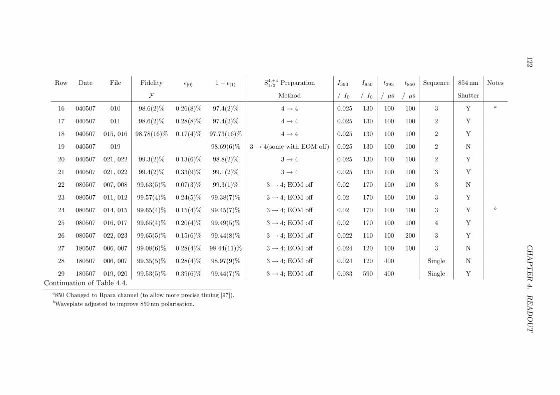
122C
HA
PT
ER
4.
RE
AD
OU
T
Row Date File Fidelity ǫ|0〉 1 − ǫ|1〉 S4,+41/2 Preparation I393 I850 t393 t850 Sequence 854 nm Notes
F Method / I0 / I0 / µs / µs Shutter
16 040507 010 98.6(2)% 0.26(8)% 97.4(2)% 4 → 4 0.025 130 100 100 3 Y a
17 040507 011 98.6(2)% 0.28(8)% 97.4(2)% 4 → 4 0.025 130 100 100 2 Y
18 040507 015, 016 98.78(16)% 0.17(4)% 97.73(16)% 4 → 4 0.025 130 100 100 2 Y
19 040507 019 98.69(6)% 3 → 4(some with EOM off) 0.025 130 100 100 2 N
20 040507 021, 022 99.3(2)% 0.13(6)% 98.8(2)% 3 → 4 0.025 130 100 100 2 Y
21 040507 021, 022 99.4(2)% 0.33(9)% 99.1(2)% 3 → 4 0.025 130 100 100 3 Y
22 080507 007, 008 99.63(5)% 0.07(3)% 99.3(1)% 3 → 4; EOM off 0.02 170 100 100 3 N
23 080507 011, 012 99.57(4)% 0.24(5)% 99.38(7)% 3 → 4; EOM off 0.02 170 100 100 3 Y
24 080507 014, 015 99.65(4)% 0.15(4)% 99.45(7)% 3 → 4; EOM off 0.02 170 100 100 3 Y b
25 080507 016, 017 99.65(4)% 0.20(4)% 99.49(5)% 3 → 4; EOM off 0.02 170 100 100 4 Y
26 080507 022, 023 99.65(5)% 0.15(6)% 99.44(8)% 3 → 4; EOM off 0.022 110 100 200 3 Y
27 180507 006, 007 99.08(6)% 0.28(4)% 98.44(11)% 3 → 4; EOM off 0.024 120 100 100 3 N
28 180507 006, 007 99.35(5)% 0.28(4)% 98.97(9)% 3 → 4; EOM off 0.024 120 400 Single N
29 180507 019, 020 99.53(5)% 0.39(6)% 99.44(7)% 3 → 4; EOM off 0.033 590 400 Single Y
Continuation of Table 4.4.
a850 Changed to Rpara channel (to allow more precise timing [97]).bWaveplate adjusted to improve 850 nm polarisation.

4.3
.E
XP
ER
IME
NT
S123
Row Date File Fidelity ǫ|0〉 1 − ǫ|1〉 S4,+41/2 Preparation I393 I850 t393 t850 Sequence 854 nm Notes
F Method / I0 / I0 / µs / µs Shutter
30 290507 009 99.03(6)% 0.14(3)% 98.2(1)% 4 → 4 0.0052 100 400 Single N a
31 290507 010 99.12(6)% 0.12(3)% 98.35(12)% 4 → 4 0.0052 100 400 Single Y
32 290507 010, 011 99.59(4)% 0.12(3)% 99.30(8)% 3 → 4; EOM off 0.0052 100 400 Single Y
33 290507 010, 012 99.68(3)% 0.12(3)% 99.47(6)% 3 → 4; EOM off 0.0052 100 400 Single Y b
34 290507 016, 017 99.70(3)% 0.17(4)% 99.58(6)% 3 → 4; EOM off 0.0052 100 400 Single Y c
35 300507 014 99.7(1)% 3 → 4; EOM off 0.0053 110 400 Single N
36 300507 014 99.5(1)% 3 → 4; EOM off 0.0053 110 100 100 3 N
37 300507 015, 016 99.1(2)% 0.1(1)% 98.2(4)% 3 → 4; EOM off 0.0053 120 400 Single Y
38 300507 017, 018 99.0(2)% 0.4(2)% 98.3(4)% 3 → 4; EOM off 0.011 230 250 Single Y
39 300507 019, 020 98.1(3)% 0.3(2)% 96.5(6)% 3 → 4; EOM off 0.021 480 150 Single Y
40 300507 021, 022 97.0(4)% 0.1(1)% 94.0(8)% 3 → 4; EOM off 0.037 880 70 Single Y
41 300507 024, 025 99.7(2)% 0.0(0)% 99.3(3)% 3 → 4; EOM off 0.0053 120 500 Single Y
42 300507 026, 027 99.7(1)% 0.2(1)% 99.5(2)% 3 → 4; EOM off 0.00027 55 1000 Single Y
43 310507 002, 003 99.77(4)% 0.11(3)% 99.64(6)% 3 → 4; EOM off 0.011 120 400 Single Y
44 310507 004, 005 99.68(3)% 0.21(3)% 99.58(5)% 3 → 4; EOM off 0.011 120 400 Single Y
45 310507 009, 010 99.70(3)% 0.18(3)% 99.58(5)% 3 → 4; EOM off 0.011 120 400 Single Y
Continuation of Table 4.4.
aExtra 850 PBS cube inserted; Pickoff removed.b397 nm Probe beam blocked. Leakage of mixed σ± light through this AOM could have contributed to optical pumping infidelities.cWaveplates adjusted to improve 397 nm σ polarisation.

124 CHAPTER 4. READOUT
than ∼ 300 µs). Although this “EOM off” pulse is of little use in qubit preparation,
it greatly reduces the contribution of S41/2 manifold preparation errors to the readout
infidelity we measure.
4.3.2.3 Some Trends
The most noticeable trend in Table 4.4 is that the greatest fidelity improvement came
from improving the population preparation (changing from 4 → 4 to 3 → 4), rather than
the readout itself. Between rows 31 and 34 ǫ|1〉 improved from 1.65(12)% to 0.42(6)%,
just by improving the state preparation; each improvement increased the fidelity. Pairs
22-23 and 30-31 are consistent with the 854 nm shutter reducing ǫ|1〉 by (a marginally
significant) ∼ 0.1% (rows 35 and 37 show an opposite, much larger effect; although
there was an hour’s gap between these two experiments and so some other parameter
could have drifted in between them). It is better to have long, low intensity pulses
than short bright ones: compare rows 38-40 with 41-44. The pulse times for rows 37-42
had been increased until ǫ|1〉 stopped improving, to ensure that they were long enough
to effectively shelve the ion. The pairs 27-28 and 35-36 suggest that the single pulse
method is more accurate than multi-pulse, although the simulations of Section 4.2 imply
that this could reverse if the sequences were properly optimised. Note that the 850 nm
beam is on for longer in total for the 400 µs single pulse than in the three 100 µs pulses
of the multi-pulse sequence. What it does show is that there are no adverse coherent
effects (such as EIT) between the 393 nm and 850 nm beams when they are on together
(at least at the 0.1% level), supporting the use of rate equations as a model.
High fidelities are seen in rows 22-26 (pulsed method, average fidelity for that day
99.63%); rows 32-34 (average 99.67%); 41-42 (99.7%) and 43-45 (99.71%). The first of
these sets used multipulse sequences, the others were single 393+850 pulses. The last of
these sets is discussed in detail in Section 4.3.2.5.
4.3.2.4 Effect of λ4 Waveplate Rotation
On 290507, the λ4 waveplates in each of the σ beams was adjusted to improve their
polarisation purity. As part of this process ǫ|1〉was recorded for a variety of waveplate
angles, for each beam in turn.
The 397 nm σ adjustment was made between rows 33 and 34 of Table 4.4. Initially
the waveplate was at 28; the best position was found to be 27 in an experiment with

4.3. EXPERIMENTS 125
25 30 350.97
0.975
0.98
0.985
0.99
0.995
1
Angle of 397σ
λ/4 Waveplate / °
Pro
babil
ity o
f D
ete
ctin
g I
on
as
Sh
elv
ed
45 55 65 75 85 95
Angle of 393
λ/4 Waveplate / °
300 310 320 330
Angle of 850
λ/4 Waveplate / °
Original Tilt
Tilted ∼5° Anticlockwise
Tilted ∼10° Anticlockwise
Figure 4.45: (1 − ǫ|1〉) as a function of waveplate angle for the three σ beams. In
all cases: the preparation method was “3 → 4; EOM off”, the 854 nm shutter was in
use, I393 = 0.0052 I0, I850 = 100 I0 and there was a single 400 µs combined 393 nm
and 850 nm shelving pulse (i.e. parameters are as rows 33 and 34 of Table 4.4). Data
points at the same waveplate angle have been displaced horizontally for clarity. The
angles are accurate to ± ∼ 1.5. For 393 and 850, simulations are shown as a curve
assuming perfect tilt. The simulations have been scaled so that the upper levels match
the experiment.
preparation method “4 → 4”. The state preparation was extremely sensitive in this
case: at 27 the probability of seeing the ion as shelved was 97.0(2)%, while 28 and 26
achieved only 96.2(3)% each. However, we see in Figure 4.45 that tuning the 397 nm
to 3 → 4, and using an EOM off pulse, greatly reduces the sensitivity to polarisation
impurity.
The 393 nm and 850 nm adjustments were made just after the experiment of row
34. The 393 nm waveplate was originally at 70, and 80 was found to be a slight
improvement – the waveplate was left in that position. The shelving seems insensitive
to the 393 nm polarisation purity (or else the purity of the beam is poor even at the
best waveplate angle). However, an earlier experiment showed that ǫ|1〉 rose by up to

126 CHAPTER 4. READOUT
10% (in that case, to 14%) when the 393 nm beam was completely σ− polarised.
For the 850 nm beam, we tried tilting the waveplate around an axis perpendicular to
the beam direction (in this case, a vertical axis). Such tilting is a well-known technique
to optimise the retardation of a waveplate. Specifically, a waveplate designed to give a
specific retardation (in this case 14 of a wavelength) can be tilted about its fast (slow)
optical axis to increase (decrease) the relative retardation [140, Section 8.7.1]. As seen
in Figure 4.45, a small anticlockwise tilt (estimated to be 5, although the rotation was
completely uncalibrated) gave an improvement of 0.25(9)% (= 99.54(6)%− 99.29(7)%).
The waveplate rotation angle was set to 314, which was its original setting.
The 393 and 850 experiments were simulated, with the laser parameters set as de-
scribed in the caption. The simulations significantly underestimate the shelving error
when the waveplate rotation is far off its optimum, particularly for the 850, for reasons
we do not understand. It might be a symptom of inaccurate power measurements, or
perhaps of the waveplates not being at the best tilt angle.
4.3.2.5 The Best Results
The highest experimentally-achieved fidelity was 99.77(4)% (row 43). This result is
statistically significantly different from rows 44 and 45 (99.68(3)% and 99.70(3)%), so
we may be justified in claiming the higher figure by itself (Figure 4.46). The experiments
of 43 and 44 were separated by ∼ 15 minutes, and we know that the 850 nm power or
polarisation purity fluctuate over this sort of timescale – the laser parameters could have
been different for the two runs, leading to the different fidelities. If we do combine the
three data sets, we obtain readout errors:
ǫ|0〉 = 0.18(2)%; ǫ|1〉 = 0.41(3)%; F = 99.706(18)%. (4.10)
This approaches the estimated target of 99.9% for an operational quantum computer
[134], although at 400 µs (plus fluorescence time) it is significantly slower than Steane
assumes in that reference (10 µs). For each of these rows, the data were collected in 40
sets of 1000 sequences (500 for row 43), 20 sets for each qubit state. Figure 4.46 shows
the errors calculated from each set individually, and it can be seen that they agree with
each other within their uncertainties. The average errors for each row are also displayed.
The optical qubit/fluorescence detection phase of the readout used a collection time
of 2 ms, a bright-state photon count rate of 7600 s−1 and a detection threshold of 3.5

4.3. EXPERIMENTS 127
0
0.002
0.004
0.006
0.008
0.01
0.012
0.014
0.016
0.018
0.021−
P(S
helv
e S
1/2
F=
4)
= ε
|1
>
0
1
2
3
4
5
6
7
8
9x 10
−3
P(S
helv
e S
1/2
F=
3)
= ε
|0
>
Row 43: F = 0.9977(4)
Row 44: F = 0.9968(3)
Row 45: F = 0.9970(3)
Figure 4.46: Readout errors from rows 43, 44 and 45 of Table 4.4, both overall (filled
symbols, to the right of the vertical gridline) and for each data subset (small dots, to
the left). The statistical uncertainties (assuming binomial distribution) are also shown
as errorbars.
photons – sequences that resulted in more counts than this were designated as “bright”.
Figure 4.47 shows the photon histograms from the experiments of row 45.
We measured the fluorescence detection using 393 nm, 866 nm and 397 nm beams
together, shelving the ion with high probability from both qubit states. The error prob-
ability was 0.04(2)% when measuring an unshelved ion and 0.16(3)% for a shelved one,
giving a total of 99.903(17)% fidelity. Removing these numbers from the results above
(all three combined), we obtain the error rate for just the shelving and state-preparation
phases:
ǫ|0〉 = 0.14(3)%; ǫ|1〉 = 0.26(4)%; F = 99.80(2)%. (4.11)
From Section 4.2.2.3 we can read directly off Figures 4.26-4.28 to see that the the-
oretical optimal shelving, for a single 400 µs pulse with the 850 nm beam at 2.3to the
magnetic field, is much higher fidelity than the experiment:
ǫ|0〉 = 0.056%; ǫ|1〉 = 0.021%; F = 99.962%. (4.12)

128 CHAPTER 4. READOUT
0 5 10 15 20 25 30 3510
0
101
102
103
104
Number of Photons Detected
Nu
mber
of
Sequ
en
ces
Prepare S1/2
3
Poisson, λ = 0.175
Prepare S1/2
4,+4
Poisson, λ = 15.2
Figure 4.47: Photon count histograms from row 45, using 2 × 10⁴ sequences for each
of S31/2 and S4,+4
1/2 . The black vertical dashed line indicates the optimum threshold. The
coloured curves show the ideal Poisson distributions, with just one free parameter (the
mean number of counts λ). The departure from the theoretical Poisson distributions
is due to a combination of shelving errors, power or frequency fluctuations of the fluo-
rescence lasers, and non-Poissonian dark-count processes in the PMT (including cosmic
rays [82]).
The intensities are I393 = 0.00320 I0 and I850 = 182 I0.
I set the simulation to use the intensities measured in the experiment (I393 = 0.011 I0
and I850 = 120 I0), and also simulated the 393 nm beam being at 2.79 to the magnetic
field, again as measured. Of these, the 393 nm intensity has by far the greatest effect.
We obtain:
ǫ|0〉 = 0.205%; ǫ|1〉 = 0.014%; F = 99.891%. (4.13)
There is still significant discrepancy with the experiment. One solution would be to
add a 16% σ− polarisation impurity to the 393 nm beam, that produces a reasonable
match to the experiment (ǫ|0〉 = 0.19%, ǫ|1〉 = 0.21%, F = 99.80%), but this seems like
an unrealistically large impurity.

4.4. FUTURE DIRECTIONS 129
We can replicate the experimental results just by changing I393 to 0.0076 I0 (30%
below the measured value, possible if the beam was misaligned, but still twice the
theoretical optimum), and adding 0.13% σ− impurity to the 850 nm beam. Both imper-
fections are very reasonable, and they are upper limits because I have assumed perfect
state preparation.
4.4 Future Directions
To further improve the experimental fidelity of readout, we would need to overcome
the current uncertainty about the experimental conditions (laser polarisations, inten-
sities etc.). We can take inspiration from Biercuk et al. [141], who demonstrate the
optimisation of a dynamic-decoupling sequence using experimental results (generated
on demand in real time) as the quantity to be optimised. A similar approach could be
used to optimise the readout fidelity, replacing the rate equations simulations.
We would need to improve the laser polarisation impurities, especially the 397 nm
σ beam. Polarisers are available (Glan-Taylor or Glan-Thompson polarisers [142]) with
claimed extinction ratios of 100 000 : 1 (compared to polarising beamsplitter cubes such
as we currently use, with claimed extinction ratios of 1000 : 1). Our polarisation purity
may in fact be limited by birefringence in the viewports of our vacuum system, but we
might be able to counteract this using carefully-set λ2 and λ
4 plates in each beam, after
the polariser. Or we might not be able to – the birefringence could change over time;
or if it varies spatially over the window, different parts of the beam would experience
different polarisation changes (on average, the polarisation state of the beam would
become mixed).
We would also need to stabilise the laser intensities. Re-routing and thermally
insulating the 850 nm fibre would help, but it may also be necessary to use noise-eaters
(the power of a beam is monitored, and this feeds back to the AOM driver to keep the
power constant). Improving the AOM extinctions (such as by detuning and reducing
the power of the driver at the same time as operating the driver’s TTL switch) would
also help.
The final requirement is a carefully thought-out optimisation procedure that can
cope with noise in the function to be optimised. Biercuk et al. [141] successfully used
the Nelder-Mead method, an optimisation algorithm that does not calculate the gradient

130 CHAPTER 4. READOUT
of the function it is optimising and is hence quite robust.
Such efforts may not be justified given that the operation of a quantum computer is
thought to be much less sensitive to the readout fidelity than to the gate fidelity.
4.5 Comparison with the Literature
In 2007 Hume, Rosenband and Wineland [85] experimentally achieved a readout fi-
delity of 99.94%, from an aluminium ion. This is almost as high as the best optimised
simulations I performed in Section 4.2.2, which assumed ideal conditions and perfect
fluorescence-detection. But the methods I have developed here are still valuable for
their simplicity and robustness. In Section 4.2.3 we saw that the multipulse shelving
method was highly resistant to changes in the 850 pulse lengths and intensities, and
relatively resistant to errors in the 393 too. The procedure can be greatly simplified, to
a single pulse with just two monochromatic laser beams, while the fidelity is barely af-
fected. The processes do not depend on coherent beams or narrow linewidths (although
the laser linewidths should not be significantly larger than the natural linewidths). And
the shelving is fast, taking just a few microseconds to reduce the the average error below
10−3.
In contrast, methods that depend on coherent processes, such as that of Hume et
al., require complex and precise pulse sequences (and in their case, a second ion). The
particular method of Hume et al. is also very slow, taking 2 ms per cycle with each cycle
having only 85% fidelity (an average of 6.5 cycles were needed to achieve their high
fidelity).
Optical qubits can be detected with very high fidelity. In 40Ca+, our group has
distinguished S1/2 from D5/2 with a fidelity of 99.9913(11)% from 40Ca+, taking ∼ 1 ms.
The 99.9% level is reached after 200 µs, and if we use an adaptive method (that only
collects data for as long as it takes to reach the desired fidelity) it is even faster [82].
The fidelity is limited by the photon collection efficiency and the D5/2 lifetime. In Ba+,
that lifetime is so long that Kurz et al. could, “completely rule out the possibility of
incorrect state determination”, by using a very long (100 ms) detection period [143].
Other experimental readout fidelities, from hyperfine ground-level qubits, that have
been reported are significantly lower than achieved in this work. One method, used
in 171Yb+ (Olmschenk et al. [57]) and 111Cd+ (Acton et al. [136], both groups at the

4.5. COMPARISON WITH THE LITERATURE 131
University of Michigan), directly applies fluorescence-detection to the qubit. Both ions
have large hyperfine splittings (12.6 GHz and 14.5 GHz in their respective S1/2 levels),
and so off-resonant excitation of the “dark” qubit state is low; and in Cd+ there are no
low-lying D-states and so a closed cycling transition can be used. There are low-lying D-
states in Yb+ but 171Yb+ has nuclear spin I = 12 , so Olmschenk et al. can repump cleanly
back to the “bright” qubit state by exploiting the fact that Fi = 0 → Fj = 0 transitions
are forbidden [57]. 111Cd+ also has I = 12 , and that selection rule (together with large
hyperfine splittings of ≈ 2 GHz in P1/2) is vital in both ions to allow a cycling transition
from clock-state qubits. Olmschenk et al. report readout with 97.9(2)% fidelity in 1 ms
[57]. Acton et al. report > 99.4% in 15 ms, and also derive theoretical results for other
ions [136]. Both methods would improve if higher photon collection efficiencies were
possible.
For ions with metastable shelves, rapid adiabatic passage is a method for directly
driving the qubit→shelf transition, with improved robustness compared to a basic π-
pulse. It works by “chirping” the shelving pulse – scanning the laser frequency over the
resonance while the amplitude is smoothly raised and lowered (e.g. a Gaussian envelope)
[144]. Wunderlich et al. used this method on S1/2 → D5/2 in 40Ca+, and achieved 99(1)%
shelving transfer in 150 µs. However they have not yet attempted state-selective shelving
from 43Ca+. A similar method is being developed with 137Ba+; so far only 60% transfer
has been achieved, but the laser is still being stabilised [145]. Benhelm notes that a
π-pulse shelving method can be made more accurate by using several pulses, each tuned
to transfer the desired qubit state to a different state in D5/2 achieving better than 99%
fidelity overall [128, 72].
The methods of this chapter – both the readout process itself and the optimi-
sation simulations – should work for other common ion species, provided that they
have low-lying D-states and a hyperfine ground-state qubit. 87Sr+, 137Ba+ and 199Hg+
might all be investigated; 137Ba+ is especially interesting because of its large S1/2 hy-
perfine splitting (8.0 GHz [145]), favourable branching ratios (Br(P3/2→D5/2) = 22%;
Br(P3/2→D3/2) = 3% [143]) and long D5/2 lifetime (≈ 33 s [146, 147]).

132 CHAPTER 4. READOUT

Chapter 5
40-43
Our group is working towards an entangling quantum phase gate between a 40Ca+ ion
and a 43Ca+ ion. The motivations behind this experiment are as follows:
• An alternative to the standard “measure-the-syndrome-and-classically-correct”
paradigm of quantum error correction involves performing classical AND gates
directly on the ions. We have designed methods to convert a 40-43 phase gate
into such an AND gate. Demonstrating the phase gate would lead naturally to an
attempt on the AND gate, and then to error-correction experiments.
• It might turn out to be preferable to use 40Ca+ rather than 43Ca+ for certain
quantum operations; but 43Ca+ clock-state qubits will almost certainly be the best
way to store quantum information as a memory. Being able to transfer quantum
information between ions of the different isotopes would be necessary in such a
case.
• With the previous 40-40 gate [75], the states |↑↓〉 and |↓↑〉 were indistinguishable.
40Ca+ and 43Ca+ can be read out independently and so complete state tomography
becomes possible [148].
To give detailed descriptions of the theory behind such a gate is beyond the scope of
this thesis [149, 150, 151, 74]. Instead I shall take a practical perspective, and describe
early experiments towards this goal. Despite significant experimental effort to realise
this gate, our attempts were unsuccessful. Diagnostic experiments to investigate the
reasons for this are described in this chapter. The eventual result was to show that our
present trap has significant failings regarding this project, and this has motivated us to
133

134 CHAPTER 5. 40-43
design and build a new apparatus for future experiments.
5.1 Introduction
Our “wobble” gate uses the method of Leibfried et al. [73], which is based on ideas from
Milburn, Schneider and James [152] and Wang, Sørensen and Mølmer [70, 153]. A more
detailed discussion can be found in [74], in the context of a two-40Ca+ ion gate; I shall
describe it qualitatively here.
5.1.1 Light-Motion Interaction
The coherent couplings between light and ion-motion can be divided into two types,
although this represents a convenient distinction of notation and imagery rather than
different physical processes (they are both derived from the same Hamiltonian [74, Sec-
tion 3.2]).
5.1.1.1 Resolved Sideband Interactions and Cooling
The first variety is the quantised simple harmonic oscillator. Each vibrational normal
mode (with angular frequency ωz) splits each existing state into a ladder of energy levels
separated by ~ωz. An atomic transition of frequency ω0 gains sidebands, of frequency
ω0 + mωz for integer m. If m > 0 (m < 0) it is a blue (red) sideband and the transition
connects |↓, n〉 with |↑, n + m〉. An example is given in Figure 5.1 that illustrates the
technique of resolved Raman sideband cooling.
The lowest temperature to which an ion can be cooled is ultimately limited by the
ion’s atomic properties [154]. The Doppler limit TD is the minimum that can be reached
by simple Doppler cooling, approximating the ion as a two-level system. The recoil limit
TR is a lower bound for any laser-cooling method, corresponding to the random recoil
“kick” the ion experiences during the spontaneous relaxation phase. For Ca+ cooled on
the 397 nm transition, and assuming an isotropic trapping potential of 500 kHz (to work
out the mean motional excitation):
TD =~
2τkB= 0.54 mK ≈ 7 quanta (5.1)
TR =h2
mλ2kB= 3.0 µK ≈ 0.04 quanta (5.2)
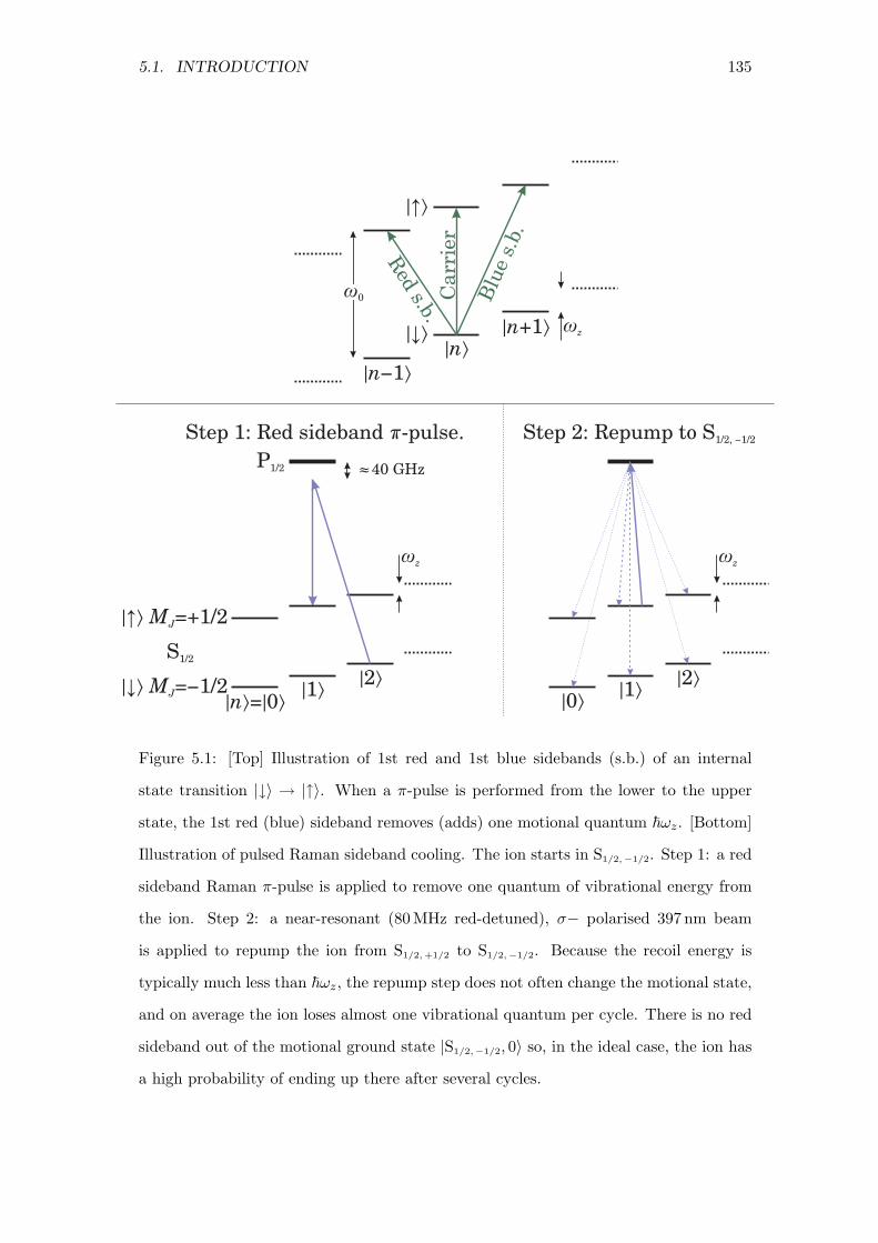
5.1. INTRODUCTION 135
Figure 5.1: [Top] Illustration of 1st red and 1st blue sidebands (s.b.) of an internal
state transition |↓〉 → |↑〉. When a π-pulse is performed from the lower to the upper
state, the 1st red (blue) sideband removes (adds) one motional quantum ~ωz. [Bottom]
Illustration of pulsed Raman sideband cooling. The ion starts in S1/2, −1/2. Step 1: a red
sideband Raman π-pulse is applied to remove one quantum of vibrational energy from
the ion. Step 2: a near-resonant (80 MHz red-detuned), σ− polarised 397 nm beam
is applied to repump the ion from S1/2, +1/2 to S1/2, −1/2. Because the recoil energy is
typically much less than ~ωz, the repump step does not often change the motional state,
and on average the ion loses almost one vibrational quantum per cycle. There is no red
sideband out of the motional ground state |S1/2, −1/2, 0〉 so, in the ideal case, the ion has
a high probability of ending up there after several cycles.

136 CHAPTER 5. 40-43
where m is the mass of an ion, τ is the lifetime of P1/2 and λ = 397 nm. Our Doppler
cooling actually achieves much higher temperatures than the limit suggests, because
we typically are not tuned precisely to the (optimal) half-fluorescence point, and use
intensities much greater than the saturation intensity, broadening the transition.
5.1.1.2 Optical Dipole Force
The second picture describes the optical dipole force. Suppose that an ionic state is
shifted by δE due to the light shift from an optical field (with a particular frequency and
polarisation). Then if the strength of the field varies with position, an ion in that state
will feel a force proportional and parallel to the amplitude gradient of the field (towards
the stronger (weaker) field if δE < 0 (δE > 0)). An example of such a spatially-varying
light field is the standing wave set up by two intersecting non-parallel laser beams of
the same frequency (see also Figure 5.2).
We use two beams derived from the same laser (397 master/slave) to ensure the
beams are mutually coherent. In fact, we set up a travelling standing wave by setting
the beams to slightly different frequencies (using the AOMs). The two beams have a
difference wavevector that lies along the trap axis, so the standing wave travels in that
direction and only affects the axial motional mode(s) of the ion(s). For now consider
just one ion with mass m (assumed to start in the ground state of motion), and suppose
the Raman beams have a difference frequency that is close to the axial frequency ωz
(detuned from it by δz). The travelling standing wave will sweep over the ion such that
the ion feels a force oscillating at frequency ωz + δz. The damping of the axial mode
is negligible and so we can treat the mode as a classical undamped simple harmonic
oscillator subject to a periodic, slightly off-resonant driving force. The ion oscillates at
ωz with amplitude modulation at δz, so it returns to rest at time t = tr = 2πδz
. We call
this a “wobble” pulse, because of the ion’s motion.
The quantum description [74, 155] is that the ion is in a coherent state |α〉, the state
that best resembles classical harmonic oscillators. Coherent states are eigenstates of the
annihilation operator a:
a |α〉 = α |α〉 , (5.3)
where α takes complex values α = |α|eiφ. The mean number of quanta in a coherent

5.1. INTRODUCTION 137
state is
〈α| N |α〉 = 〈α| a†a |α〉 = |α|2. (5.4)
The position and momentum (here using the operators in the Heisenberg picture) have
expectation values
〈α| z(t) |α〉 = 〈α|√
~
2mωz(a†eiωzt + ae−iωzt) |α〉 = 2|α|z0 cos(ωzt − φ) (5.5)
〈α| p(t) |α〉 = 〈α| i√
m~ωz
2(a†eiωzt − ae−iωzt) |α〉 = −2|α|z0mωz sin(ωzt − φ) (5.6)
where
z0 =
√
~
2mωz, (5.7)
which shows how the coherent state resembles the classical harmonic oscillator.
As the ion is driven by the travelling standing wave wobble pulse, α(t) travels round
a circle in the complex plane (equivalently, round a circle in z-p phase space, in a frame
rotating at ωz). It starts at zero (the ground state), returning to zero at time tr = 2πδz
.
The ion’s overall wavefunction gains a phase Φ proportional to the area of this circle:
after a single complete cycle we have
Φ(tr) = −π
2
(
Fm
δz
)2
. (5.8)
The amplitude of the dipole force is Fm = ηΩ = δkz0Ω where η is the Lamb-Dicke
parameter, δk is the difference between the wavevectors of the two beams, and Ω is the
Rabi frequency.
By itself this phase is uninteresting, because global phases are irrelevant in quantum
mechanics. But we could start with the ion in a superposition of states, such that each
state feels a different light shift and thus a different value of Fm. Each component of the
superposition picks up a different phase shift, and so the travelling standing wave acts
as a single-qubit phase gate. Of course, simpler phase gates are available that are faster
and have higher fidelities – such as applying a single laser beam to provide a constant
differential light shift between the qubit states. But the above process generalises easily
to a two-qubit controlled-phase gate.
5.1.1.3 Same-Species Gate
Two 40Ca+ ions are trapped in the same potential, so there are now two axial modes
of the ions moving collectively: centre-of-mass motion (CoM) with frequency ωz and

138 CHAPTER 5. 40-43
stretch motion (Str) at ωz
√3. Each of these modes behaves as described above. The
light field is set up so that S1/2, +1/2 and S1/2, −1/2 experience opposite light shifts. The
ion spacing is carefully set so that it is an integer number of wavelengths of the standing
wave (Figure 5.2). So at any time, the ions feel forces of equal magnitude – in the same
direction if both ions are in the same internal state, in opposite directions if they are in
different internal states. The Raman beams’ difference frequency is chosen to be close
to the Str frequency (ωz
√3 + δz) – being far off resonant from the CoM mode means
that only the Str is significantly excited. And the Str mode is only excited when the
ions feel oppositely directed forces, when they are in different states. Only in that case
will the travelling standing wave be able to drive the Str oscillation, and thus give the
ions (collectively) a phase shift Φ as given by (5.8). Careful choice of δz provides Φ = π2 ,
and so we achieve the controlled phase gate
G40−40 =
1 0 0 0
0 i 0 0
0 0 i 0
0 0 0 1
. (5.9)
In previous work our group implemented this gate with fidelity 83% [75].
Figure 5.2: Illustration of two ions in a travelling standing wave, spaced a whole number
of wavelengths apart. In this case they are assumed to be in the same internal state,
and so experience equal forces F in the same direction. White arrows indicate the beam
directions.

5.1. INTRODUCTION 139
There are several subtleties to implementing the gate; such as ensuring that the
static light shifts induced by each Raman beam are equal for both qubit states (to
reduce single-qubit phase shifts). To cancel out other single-ion phase shifts (such as
magnetic field drift, or the static two-photon light shift), we do a spin-echo sequence
on both ions. The wobble pulse is divided into halves, placed symmetrically on either
side of the spin-echo π-pulse (similar to Figure 5.6). The π-pulse reverses the direction
with which the qubits precess with respect to single-ion light shifts, unwinding the
accumulated unwanted phase. But the collective effect of the wobble pulse depends on
the relative spin-state of the ions (both the same or both different), and so the wobble
phase is summed over both pulses and the two-qubit gate works. See Dr. Home’s thesis
for very full details [74].
5.1.1.4 Mixed-Species Gate
The two-qubit gate G can be applied to a mixed crystal of 40Ca+ and 43Ca+. In this case
the ions have different atomic structure – in particular, very different qubit frequencies
of ∼ 5 MHz and ∼ 3 GHz respectively. Nevertheless, the gate should still work because
the oscillating force is applied close to the trap frequency 1.702ωz1, and is independent
of the qubit frequencies. The ions will respond differently to the light field; the forces are
different in magnitude for each ion, and for each of the four possible two-qubit states.
It also becomes impossible to cancel out the single qubit phase shifts: assuming typical
beam parameters, if the 40Ca+ light shifts are balanced then the 43Ca+ qubit states
are differentially shifted by ∼ 30 kHz [149]. But by separating two gate pulses with
single-qubit carrier π-pulses, we can ensure that the gate reduces to G40−40.
5.1.2 Mixed-Isotope Readout
To show that our gate leaves the ions entangled, we must be able to read-out from
both ions at the end of each sequence. The large isotope shift between the ions, and
the hyperfine structure of 43Ca+, allow us to stimulate and detect fluorescence from
each ion separately. 40Ca+ fluoresces ∼ 5 times more strongly than 43Ca+ under the
experimental conditions, and so uses a shorter counting period; 40Ca+ fluorescence is
1The Str frequency for two 40Ca+ ions is ωz
√3 ≈ 1.732ωz, where ωz is the centre-of-mass frequency;
the small mass difference between 40Ca+ and 43Ca+ changes the vibrational modes slightly. For the
40-43 crystal, the Str frequency ωs,40−43 = 1.702ωz and the CoM frequency ωc,40−43 = 0.981ωz [149].

140 CHAPTER 5. 40-43
done first to minimise error due to decay of the D5/2 shelf.
The ions are shelved using a single pulse containing both 393 nm σ+ and 850 nm
σ−. 1.938 GHz sidebands are imposed on the 393 nm beam using an EOM so that when
the carrier frequency is resonant with 40Ca+, the upper sideband excites the S41/2 → P5
3/2
transition in 43Ca+. This allows it to shelve from both ions simultaneously. The 850 nm
beam is tuned and polarised for EIT readout of 40Ca+ (see Figure 4.1), and the pulse time
is set for highest fidelity from that ion (up to ∼ 90%). Then the 43Ca+ readout fidelity
reaches ∼ 90% without further adjustment. It seems likely that further optimisation
would allow higher fidelities. Figure 5.3 shows a test with simultaneous Rabi oscillations
of 43Ca+ and 40Ca+.
At the end of each sequence, the ions are deshelved by the 854 nm beam tuned
in-between the isotopes’ resonances.
0 5 10 15 200
0.1
0.2
0.3
0.4
0.5
0.6
0.7
0.8
0.9
Microwave or Raman Pulse Time
Fra
ctio
n o
f P
op
ula
tion
Sh
elv
ed
40Ca
+; Time / µs
43Ca
+; Time / 10µs
Figure 5.3: Independent carrier oscillations of 43Ca+ (using microwaves) and 40Ca+ (us-
ing Raman laser beams) with Rabi frequencies 5.4 kHz and 95 kHz respectively, testing
the simultaneous readout. The horizontal time axis is shared by both plots, but note
the ×10 scaling factor for 43Ca+.

5.1. INTRODUCTION 141
5.1.3 Pulse Sequence
Figures 5.4-5.6 show an experimental pulse sequence for testing the 40-43 wobble gate.
The sequence has several phases.
Dop
ple
r co
oli
ng
(Low
39
7 p
ow
er)
Con
tin
ou
s R
am
an
cooli
ng
Pu
lsed
Ra
ma
n c
ooli
ng (
*)
Sta
te p
rep
ara
tion
Ga
te e
xp
eri
men
t (*
*)
Sh
elv
ing
Flu
ore
scen
ce d
ete
ctio
n (
Ca
)4
0+
Sh
utt
er
op
en
dela
y
Flu
ore
scen
ce d
ete
ctio
n (
Ca
)4
3+
Desh
elv
e
Ch
eck
flu
ore
scen
ce
1. Cooling 2. Experiment 3. Readout
Figure 5.4: Pulse sequence for a 40-43 experiment. See Figures 5.5 and 5.6 for expanded
views of the sections marked (*) and (**).
1. Cooling
(a) Doppler cooling. To reduce the final temperature achieved by Doppler
cooling, the 40Ca+ 397Doppler beam is reduced in power narrowing the effec-
tive linewidth. It is returned to normal at the end of this 1.5 ms pulse (using
the “Set DAC (fixed)” instruction).

142 CHAPTER 5. 40-43
Con
tin
ou
s R
am
an
cooli
ng
Sta
te p
rep
ara
tion
CoM
red
sid
eban
d
π-p
uls
e
Rep
um
p
Str
red
sid
eban
d
π-p
uls
e
Rep
um
p
Figure 5.5: Detail of Figure 5.4, showing the pulse sequence for pulsed Raman sideband
cooling.
(b) Continuous Raman cooling. We cannot perform pulsed Raman cooling
immediately after Doppler cooling, because the Doppler temperature is not
low enough. The ions could have a high motional excitation that could not be
efficiently cooled by the pulsed method. So we use 5 ms of continuous Raman
sideband cooling. The 397 Probe and Sigma AOMs (Figure 2.6) have their
frequencies set so that the beams can drive the CoM and Str red sidebands.
The 397σ beam itself repumps out of S1/2, +1/2 (Figure 5.1); it is ≈ 90 MHz
red-detuned, so the rate is small enough that the Raman transitions can
occur. By applying the beams continously, this method can efficiently cool
from a wide range of initial motional states.
(c) Pulsed Raman cooling. Continuous cooling reduces the Com and Str

5.1. INTRODUCTION 143
Sta
te p
rep
ara
tion
Flu
ore
scen
ce d
ete
ctio
n (
Ca
)40
+
43
+C
aR
ab
i fl
op
pin
g
(va
ria
ble
len
gth
02
π)
→
40
+C
aπ
/2-p
uls
e
40
+C
aπ
/2-p
uls
e (
va
ria
ble
ph
ase
)
40
+C
aa
nd
spin
-ech
oπ
-pu
lses
43
+C
a
Fir
st h
alf
of
“wob
ble
”ga
te p
uls
e
Seco
nd
ha
lf o
f“w
ob
ble
”ga
te p
uls
e
43
+C
aπ
/2-p
uls
e
Sh
elv
ing
Figure 5.6: Detail of Figure 5.4, showing the pulse sequence for a wobble gate test.
excitations to n . 3, and it is feasible to perform pulsed Raman cooling. We
repeatedly apply the following sequence ∼ 20 times:
i. CoM red sideband ∼π-pulse (18–38 µs)
ii. 397σ repump
iii. Str red sideband ∼π-pulse (35–50 µs)
iv. 397σ repump
The sideband pulses are driven by R‖ and R63 (see Figure 2.5). The fre-
quencies are measured in advance by a scan similar to Figure 5.12 below; the
Marconi synthesizers (3 and 4, Figure 2.7) are set to these frequencies and
the X and Y switches are used to select the relevant frequency for each pulse.

144 CHAPTER 5. 40-43
The π-pulse times are then measured on each sideband, and the sequence
set appropriately. Since the Rabi frequency falls as n falls, we add cooling
pulses to the sequence in groups of five, measure the π-time after each change
and use the result as the pulse time of the next group. We get best results
by interleaving CoM and Str pulses. Figure 5.5 shows the pulsed cooling se-
quence from Figure 5.4 in more detail. During these experiments we achieved
temperatures down to n ∼ 0.1 (although n ∼ 0.3 was more common).
Note that both Raman cooling methods act only on the 40Ca+ ion; the 43Ca+
is a mostly inert spectator. More information about this “sympathetic” cool-
ing can be found in [93].
2. Experiment. In this phase we perform the actual experiment, which could be a
measurement of motional coherence or heating rate, or a test of the wobble pulse
as shown in Figure 5.6. The wobble pulse is split into two parts, applied either
side of a spin-echo π-pulse on each ion, to cancel out single-ion phase shifts. The
variable-length microwave pulse allows the 43Ca+ state to be chosen, and then
the gate attempts to transfer the state to the 40Ca+ so that Ramsey interference
fringes are observed as the microwave pulse length is scanned. Also shown are the
“Set DAC” instructions that allow us to scan the phase of the final π2 -pulses, for
tomography of the entangled state [74].
3. Readout. As described in Section 5.1.2.
5.2 Crystal issues and Ion Ejection
5.2.1 Crystallisation
Crystallising a 40-43 pair has always been difficult, and it subjectively seemed much
worse during the time of these experiments. On good days, the ions would be in a linear
axial crystal but would swap positions with frequency of order once per 3 minutes. We
normally try to keep the ions in the same position during an experiment, so that they
feel the same laser intensities (it is often easy to tell what position they are in, because
they give different count rates even with the PMT). Sometimes it will subjectively be
very hard to crystallise the ions – they will exist in a cloud, or in a “pseudo-crystal”
such as the cigar shape described below. “Pseudo-crystals” appear well localised on the
5.2. CRYSTAL ISSUES AND ION EJECTION 145
camera, as opposed to clouds that are often almost invisibly diffuse. They also have
much higher count rates than clouds – sometimes as much as an axial crystal if the
397 nm Doppler beam is a little red-detuned.
Left-Hand and Right-Hand Crystals These are the desired axial crystals, named
for the position of the 40Ca+ ion as seen on the camera images.
Cigars “Cigars” is the name we have given to various pseudo-crystals that lie axially
like a proper crystal, but in which the ions are in motion so that the camera
shows a single elliptical blob. Cigars come in various lengths, and they might be
qualitatively different: we watched short (≈ 5 pixels on camera) cigars turn into
longer ones (≈ 6 pixels), with the latter having 30% higher fluorescence, and the
change between the two configurations taking 7 s one time and ∼ 0.5 s another.
Sometimes long cigars look peanut-shaped.
Line of Sight Pseudo-Crystal The ions appear to be aligned radially in the trap,
one behind the other in the line-of-sight of the imaging system. They look like a
single blob on the camera, slightly larger than a single ion appears, at the location
expected for a single ion. If the fluorescence laser is switched between exciting
40Ca+ and 43Ca+, the blob is visible for both isotopes and it does not move
significantly (i.e. it is not the case that one of the ions is hot and in a large orbit
that is not visible). We cannot tell whether, if this pseudo-crystal was viewed from
the side, it would look like a proper crystal or like a cigar.
Figure 5.7 shows some of these situations.
5.2.2 Ion Ejection
In the week starting 25th August 2008, we had great trouble loading the trap. Ions
would vanish for very little reason. It was very hard to add a single 40Ca+ to a 43Ca+;
we often got two 40Ca+ ions (which very rarely happens normally). Then, for a few
days, 40Ca+ ions would often vanish from the trap while leaving the 43Ca+. There
would often be no noticeable problem with any lasers, and we could not satisfactorily
pin the problems on variability of the RF trap drive amplitude (which we monitored).
It was during this period that I made the electrode noise measurements of Section
5.3. Over the next few days, the problem gradually went away, until by 9th September

146 CHAPTER 5. 40-43
Approximate
trap centreTrap axis ( )z
Figure 5.7: Some images of crystals and pseudo-crystals, for 40-43. Endcap voltages
240 V and 238 V; RF amplitude 140 Vpk−pk (≈ 700 mVpk−pk on monitor); axial frequency
ωz ≈ 2π × 475 kHz; radial frequency ωr ∼ 2π × 700 kHz.
2008 we were doing single-40Ca+ Raman pulsed sideband cooling (heating rate a few
hundred quanta/s).
5.3 Electrode Noise and RF Harmonics
5.3.1 RF Correlation
If a trapped ion is not located precisely at the null point of the radio-frequency (RF)
electric field, it will experience an oscillating force at that frequency. The resultant
motion is called micromotion, and we avoid it by using DC electric fields to adjust the
position of the ion onto the null point. We detect micromotion by photon arrival-time
correlation. The ion is made to fluoresce with the Doppler cooling beams, with the

5.3. ELECTRODE NOISE AND RF HARMONICS 147
397 nm beam detuned near the half-fluorescence point. The computer records the time-
of-arrival of photons detected by the PMT, and counts them in bins based on the phase
of the trap RF at the arrival time. When micromotion forces the ion towards (away
from) the oncoming beam, it will be Doppler-shifted closer to (further from) resonance
and the count rate will increase (decrease). The computer plots a graph of counts vs. RF
phase, and the shape of the graph allows us to tune the voltage on the DC compensation
electrodes to minimise the micromotion. As well as the usual horizontal 397 nm Doppler
beam, we have a vertical beam so that we can detect micromotion along both radial
axes (we expect negligible micromotion along the axial direction).
During this series of experiments, RF correlation scans showed a high frequency,
small amplitude oscillation (Figure 5.8, bottom). This is seen in horizontal and vertical
directions, even when optimally compensated, with single 40Ca+ and with 40-43, and for
both Left- and Right-Hand crystals and Line-of-Sight. Fitting sine functions to various
correlation scans shows that this is an oscillation at five times the RF frequency (i.e.
32 MHz). It must be phase-coherent with the RF to show up in the scans.
5.3.2 RF Harmonics
We have looked at the trap RF, and the DC electrodes, using oscilloscopes and a spec-
trum analyser to look for harmonics of the RF. The RF does have harmonics, but the
fifth harmonic is not especially strong (19 dB below the fundamental, Figure 5.9) as the
correlation results might suggest. The DC electrodes also seem to pick up the RF and
harmonics – with the harmonics relatively stronger. For instance, using a spectrum anal-
yser connected (via a 500 Hz high-pass filter) to the cable between the high-voltage DC
supply and the feedthrough, the fundamental and third harmonic both reach −10 dBm
(Figure 5.10).
5.3.3 Electrode Noise
In 2003 Jonathan Home [156] used a spectrum analyser to measure noise near the trap
axial frequency (500 kHz) picked up by the trap’s DC electrodes from the trap RF. I
repeated this measurement on 29th August 2008, and found that noise levels had not
increased.
The spectrum analyser’s 50 Ω input was connected to the BR/BL cable – this is a
coaxial cable whose central conductor is attached to the BR trap DC electrode, and the

148 CHAPTER 5. 40-43
0 50 100 1500
50
100
150
200
250
Time relative to trap RF cycle / ns
PM
T C
ou
nts
0 50 100 1500
500
1000
1500
2000
2500
3000
3500
Time relative to trap RF cycle / ns
PM
T C
ou
nts
Horizontal Beam
Vertical Beam
Figure 5.8: RF Correlation scans for a single 40Ca+ ion. There is ≈ 3% uncertainty
in the horizontal axis scale. Trap RF period is 157 ns. [Top] Normal scan (horizontal
Doppler beam) showing oscillation at the RF frequency fRF. The ion’s vertical position
is not optimal. [Bottom] Scans with horizontal and vertical beams, showing anomalous
5 × fRF oscillation. No visible oscillation at fRF because the ion is well compensated.

5.3. ELECTRODE NOISE AND RF HARMONICS 149
−10 −8 −6 −4 −2 0 2 4 6 8
x 10−7
−100
−50
0
50
100
Time / s
Volt
age / V
pk
−p
k
100
101
102
103
10−1
100
101
102
103
104
Frequency / MHz
Rela
tive A
mp
litu
de
Figure 5.9: [Top] Trap RF Monitor output sampled by oscilloscope. [Bottom] Fourier
transform of trap RF. The RF frequency is 6.364(10) MHz – this frequency and its
harmonics are marked as solid black vertical lines.
shield to the BL electrode. The BR electrode is usually used as the microwave antenna
(the microwave amplifier was disconnected for this test). For each value of the trap RF
amplitude, the spectrum analyser was set to a variety of resolution bandwidths (10 Hz
to 10 kHz) and the power at 500 kHz was measured. This procedure was repeated for
several settings of the trap RF, and also with the analyser’s 50 Ω input terminated –
this latter measurement shows the analyser’s noise floor, which was subtracted from all
the other measurements.
I made two measurements with the RF switched off. They were almost indistinguish-
able from the noise floor, so they are not included with the rest of the results in Table
5.1 and Figure 5.11. The power per unit bandwidth was found by fitting straight lines
to a log-log plot of the data: let P be the power measurement and b be the bandwidth,
then the fit
log10(P ) = m log10(b) + c (5.10)
implies
P = 10cbm (5.11)

150 CHAPTER 5. 40-43
−100
−80
−60
−40
−20
0
Pow
er
/ d
Bm
100
101
102
−100
−80
−60
−40
−20
0
Frequency / MHz
Pow
er
/ d
Bm
RF On
RF Off
Figure 5.10: Trap RF and harmonics as picked up by the Near Endcap and measured
with a spectrum analyser. RF amplitude was 145 Vpk−pk. Four sweeps were made with
the analyser, for different frequency ranges (the different coloured lines). A −20 dB
attenuator was used for the two ranges highest in frequency – their traces have been
adjusted for this. The measurements were made for RF on and off. The RF frequency
(6.364 MHz) and its harmonics are marked as solid black vertical lines.
where 10c is the power per unit bandwidth. m was equal to 1 within the uncertainty
of the fit for all the data except for 160 Vpk−pk (m = 1.08(3)) and the noise floor
(m = 1.015(11)).
Jonathan performed measurements up to 180 Vpk−pk, whereas the maximum RF
amplitude I could obtain was ≈ 166 Vpk−pk. This could possibly be a sign of degradation
of the Colpitts oscillator that drives the RF. But since there is perhaps less noise now
than in 2003, it seems that the oscillator is not to blame for our current problems.

5.4. RAMAN MOTIONAL SPECTRA 151
RF Voltage in Vpk−pk Power per unit bandwidth = 10c / aW Hz−1
Jonathan Home [156] This Work
0 1.1
60 1.9(7)
90 4.7 3.7(8)
110 5.1(7)
160 7.7(1.3)
180 21
Table 5.1: Noise power as picked up by the trap’s DC electrodes. The spectrum anal-
yser’s noise floor (2.01(14) aW/Hz for this work; 3.97 aW/Hz for [156]) has been sub-
tracted.
5.4 Raman Motional Spectra
5.4.1 Observation of Radial Mode in Axial Motion-Coupling Raman
Scans
During previous experiments, a “mystery-mode” was sometimes observed in Raman
sideband frequency scans, when a mixed crystal or two 40Ca+ ions were being used. We
observed this mode during the current experiments, both in a mixed crystal and with
a single 40Ca+. An example scan is shown in Figure 5.12. We have good evidence that
this is the radial oscillation mode – it varies with the trap’s RF voltage, and matches
radial secular frequencies found by tickling (see Section 2.2.1).
We do not understand how we manage to excite the radial mode with Raman beams
that should be very well aligned with the trap axis (∼ ±3). It has of order half the
Rabi frequency of the axial modes (e.g. a single 40Ca+ with ωr = 2π × 580 kHz and
ωz = 2π×470 kHz: radial sideband π-pulse time tπ,r = 35 µs and axial sideband π-pulse
time tπ,z = 14 µs with continuous Raman sideband cooling only; tπ,z = 24 µs when
nz ≈ 0.16).
5.4.2 Heating Rates
The temperature of a vibrational mode can be measured from Raman sideband scans
such as Figure 5.12. Let R be the height of the red sideband peak divided by the height
of the blue sideband peak (the heights are measured above the shelving baseline in that

152 CHAPTER 5. 40-43
0 20 40 60 80 100 120 140 160 1800
0.005
0.01
0.015
0.02
0.025
Trap RF / V pk−pk
Pow
er
per
un
it B
an
dw
idth
at
50
0k
Hz i
n f
W/H
z
Nois
e F
loor
Su
btr
act
ed
DJS 29th August 2008
JPH 2003
Figure 5.11: Noise power as picked up by the trap’s “BR” DC compensation electrode.
The spectrum analyser’s noise floor (2.01(14) aW/Hz for this work; 3.97 aW/Hz for [156])
has been subtracted. Similar recordings were made from the endcap electrodes.
part of the scan). Then the mean occupation of that mode is n quanta where [74]
n =R
1 − R. (5.12)
By doing one scan with the measurement immediately after sub-Doppler cooling, and
another scan with a delay between the cooling and the measurement, we can measure the
rate at which the ion heats up. Such heating can be caused by noise on the electrodes,
photon scattering, collisions with gas molecules etc.
During the last three months of 2005, the heating rate of a single 40Ca+ ion was
measured more than thirty times [74]. The heating rate was usually less than 10 quanta
per second (qps). Sometimes, for reasons unexplained, it would rise to 10s of qps, the
highest measured rate being ≈ 200 qps.
We measured the heating rate of a 40-43 crystal on 24th July 2008. The Str (CoM)
mode heating rate was found to be ≈ 180 qps (≈ 570 qps). A similar, measurement on
20th August found ∼ 150 qps (∼ 200 qps). We qualitatively expect the Str mode to be
less susceptible to heating than the CoM, because the ions are so close together that

5.4. RAMAN MOTIONAL SPECTRA 153
−800 −600 −400 −200 0 200 400 600 8000
0.1
0.2
0.3
0.4
0.5
0.6
0.7
Raman Difference Frequency / kHz
Fra
ctio
n S
helv
ed
Data
Radial Frequency
Axial Frequency
Figure 5.12: Raman sideband scan of a single 40Ca+ ion, showing axial and radial
sidebands. The ion was first cooled with forty sideband cooling pulses, and then prepared
in the unshelved qubit state. A Raman probe pulse of tπ,z = 28 µs was then applied,
followed by readout. 200 sequences were performed for each frequency setting of the
Raman probe. The carrier (no motional component) is at 0 kHz and highly overdriven.
The dashed vertical lines show the location of the axial sidebands at ±470 kHz (measured
using the blue sideband; the red sideband is not visible because the ion is cold, mean
axial vibrational excitation nz < 0.3). The solid vertical lines show the positions of the
radial sidebands, measured by tickling to be 604 kHz. The sidebands are approximately
equal heights, showing that the radial mode is hotter than nr & 3.

154 CHAPTER 5. 40-43
small changes in the electric field affect them equally
For a single 40Ca+ ion, three measurements found the ion heating rate to be ≈
200 qps, ≈ 20 qps and ≈ 80 qps on 9th and 11th September. The heating rate thus
seems to be greater than in 2005.
5.4.3 Motional Coherence
It is possible to measure the coherence time of the vibrational states using a Ramsey
sequence. The ion is cooled, prepared in an equal superposition of qubit states, and
has a blue sideband π-pulse applied. After a variable delay time, the sideband pulse is
applied again. Then we apply a carrier π2 -pulse whose phase is scanned, and finally the
state is read out. The result is Ramsey fringes whose amplitude (as a function of the
delay time) reveal the decoherence rate. See [74] for details.
For a single 40Ca+, our measurement of the coherence time was ≈ 6 ms for axial
frequency 470 kHz (The figure in [74] was 76(30) ms – more than ten times better). We
also did this for a mixed crystal (coherent manipulations were only applied to 40Ca+,
with 43Ca+ being a spectator). Then the Str (CoM) mode had coherence times of
0.186(7) ms (160(60) ms). This contrasts sharply with the heating rate measurements,
where the CoM was found to heat more strongly than the Str mode. We would also
expect the CoM to decohere faster. We do not know what could cause the CoM coherence
to be so much longer in this measurement (based on delays of up to 10 ms), nor why our
single 40Ca+ measurement is much worse than previously.
One source of decoherence of the Str mode is given by Roos et al. [157]. They
show that the ions’ radial motion – specifically the antiphase “rocking” modes – couples
to the axial motion in a mathematically similar way to Kerr nonlinearities in optics.
The ampltitude of the rocking motion affects the ions’ mean separation, and hence the
Coulomb force between them. Each additional quantum in a rocking mode changes the
Str frequency, and Roos et al. detected this in experiments. Specifically: let the radial
trap frequency be ωx = ωy; let the angular frequencies of the CoM, Str and rocking
modes be ωz, ωs = ωz
√3 and ωk =
√
ω2x − ω2
z respectively; let nk,x and nk,y be the
numbers of phonons in the two perpendicular rocking modes; let α be the fine structure
constant, m be the ionic mass and c the speed of light; then the “cross-Kerr coupling

5.4. RAMAN MOTIONAL SPECTRA 155
constant” χ is
χ = −ωs
(
1 +ω2
s
8ω2k − 2ω2
s
)
ωz
ωk
(
2~ωz
α2mc2
) 13
(5.13)
and the shift in the Str frequency is
δωs = (nk,x + nk,y + 1) χ. (5.14)
Their experiments found the shift to be significantly lower than this theory predicts.
For our experiments, taking ωz = 2π × 460 kHz and ωx = 2π × 750 kHz, we get χ =
−11 Hz × 2π. To give a coherence time of ≈ 0.2 ms would require the rocking modes
to have a total of ∼ 200 quanta, while we expect Doppler-cooling to leave the ions at
0.5–2 mK implying 6–25 quanta in these modes.
5.4.4 Schrodinger Cats
Let us return to the single-qubit geometric phase gate described in Section 5.1.1.2.
Previously we only considered the case where the coherent state returned to |α = 0〉 at
the end of the wobble pulse that creates the travelling standing wave. But suppose the
wobble pulse duration t did not equal the return time tr = 2πδz
. Then the two parts of the
wavefunction (that were originally the qubit states |↑〉 and |↓〉) will have very different
values of |α〉. Such a state – being superpositions of two states that are “far apart” in
some parameter – is often called a Schrodinger Cat state. The overlap integral between
the parts will be small if they have large motional excitations. Therefore, if the wobble
pulse is placed in the gap of a Ramsey experiment, the fringe contrast will be low except
for t ≈ tr.
We performed Schrodinger Cat experiments to try to diagnose possible problems
with our wobble pulses when we could not make the two-qubit gate work. A Ramsey
spin-echo sequence (scanning the phase of the final π2 -pulse) had a detuned wobble pulse
of length t in its first gap. For a single 40Ca+, plotting Ramsey fringe contrast A against
t gives Figures 5.13 and 5.14. Both sets of data are fitted with the function [74]:
A = ne−γte−2|αA|2
(
sin(
δefft
2
))
(5.15)
where: n is a normalisation constant (that includes imperfect readout etc.); γ is a
phenomenological decay constant; |αA| =√
n + 1/2|∆α| indicates how far apart the
superposed states become in phase space; δeff is approximately the detuning of the

156 CHAPTER 5. 40-43
travelling standing wave from the motional frequency (it is not exact because large
motions cause the ions to leave the Lamb-Dicke regime [158]); tr,eff = 2πδeff
. Table 5.2,
and the figures that follow, show the data and the fits.
Figure Ion(s) Set δ/2π γ / s−1 |αA| δeff/2π tr,eff
/ kHz / kHz / µs
5.13 40Ca+ 10 1800(300) 1.72(2) 11.680(10) 85.6
5.14 40Ca+ 15 2900(400) 1.257(16) 16.28(6) 61.4
5.15 40Ca+&43Ca+ 10 9700(300) 0.668(7) 9.94(15) 100
5.16 40Ca+&43Ca+ 10 22200(500) 1.26(4) 11.50(14) 87
5.17 40Ca+&43Ca+ 34 7400(600) 0.93(4) 12.28(10) 81
Table 5.2: Parameters from recent Schrodinger cat experiments. The first two rows use
single 40Ca+ ions; the last three rows used 40Ca+–43Ca+ two-ion crystals.
0 20 40 60 80 100 1200
0.05
0.1
0.15
0.2
0.25
0.3
0.35
0.4
t / µs
Fri
nge C
on
tra
st
Figure 5.13: Schrodinger cat experiment with a single 40Ca+ ion. δ = 2π × 10 kHz.
The single 40Ca+ experiments are of a similar quality to those in [74]. For instance,
in two experiments with δ = 2π × 10 kHz he finds γ = 3500 s−1 and γ = 2000 s−1, and
αA = 1.49 and αA = 1.44; which are all of the same order as the first two rows of Table
5.2.

5.5. CONCLUSION 157
0 10 20 30 40 50 60 70 800
0.05
0.1
0.15
0.2
0.25
0.3
0.35
0.4
t / µs
Fri
nge C
on
tra
st
Figure 5.14: Schrodinger cat experiment with a single 40Ca+ ion. δ = 2π × 15 kHz.
However, it is immediately apparent that the 40-43 experiments are extremely poor.
The return of coherence, seen so clearly in the single ion results, is of much lower ampli-
tude, presumably because of the very high decoherence rate of the Str mode compared
to a single ion. Also note that for the final row (Figure 5.17), where δ = 2π × 34 kHz
from the Str mode, the second peak is expected at ∼ 30 µs. Instead it seems delayed
until ∼ 80 µs.
5.5 Conclusion
The Str coherence time of ∼ 200 µs is too short to allow high-fidelity motional operations
with the 40-43 crystal, and is probably responsible for the failure of our attempts at the
gate. A serious practical problem is decrystallisation of 40-43 pairs. This impedes all
work with the ions, including experiments to find the source of the motional decoherence.
Our current opinion is that some unknown electrical problem causes decrystallisation,
and possibly the decoherence too. We have tried grounding the electrode power sup-
plies to various different positions, or leaving them floating, in attempts to eliminate
ground loops. We were unable to produce a consistent improvement. Also, physically

158 CHAPTER 5. 40-43
0 20 40 60 80 100 1200
0.05
0.1
0.15
0.2
0.25
0.3
0.35
0.4
t / µs
Fri
nge C
on
tra
st
Figure 5.15: Schrodinger cat experiment with a 40-43 pair. δ = 2π × 10 kHz from Str.
manipulating the coaxial cables to the DC electrodes was often enough to eliminate the
pickup of low-frequency noise from that electrode, or cause the ions’ crystallisation state
to change.
For some time, the group has aimed to replace the current trap with a new one
(as described in Section 7.1). This would be of the same basic design but a factor of
2.4 smaller (ion to RF electrode distance), allowing tighter confinement of the ions. In
particular, we expect to be able to reach higher axial frequencies (allowing easier ground-
state cooling, without the need for continuous Raman cooling) and have a tighter radial
potential to reduce decrystallisation. We have decided to invest our efforts on this new
apparatus rather than attempt to solve the problems in the current system.
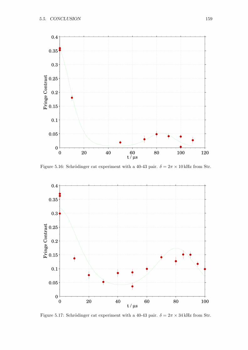
5.5. CONCLUSION 159
0 20 40 60 80 100 1200
0.05
0.1
0.15
0.2
0.25
0.3
0.35
0.4
t / µs
Fri
nge C
on
tra
st
Figure 5.16: Schrodinger cat experiment with a 40-43 pair. δ = 2π × 10 kHz from Str.
0 20 40 60 80 1000
0.05
0.1
0.15
0.2
0.25
0.3
0.35
0.4
t / µs
Fri
nge C
on
tra
st
Figure 5.17: Schrodinger cat experiment with a 40-43 pair. δ = 2π × 34 kHz from Str.

160 CHAPTER 5. 40-43

Chapter 6
Dynamic Decoupling
The use of spin-echoes [159] to improve the coherence of a quantum state is well known
[58, 62]. A set of qubits, each in a superposition state, will accumulate phase offset
errors if they precess at slightly different frequencies. This decoherence (or, more pre-
cisely, dephasing), is clearly a problem if the qubits are part of some quantum memory.
Inserting a π-pulse in the middle of the storage time can “unwind” the excess phase
acquired due to this frequency difference, and restore the quantum information at the
end of that time. However, if the frequency offsets vary with time, the acquired phases
will no longer be equal-and-opposite in the two halves of the storage delay, and there
will be uncorrected errors in the stored information.
In this chapter I derive a pulse sequence that can correct for such time-varying
frequency errors. In the literature this is called “dynamic decoupling”, to distinguish it
from the situation that often obtains in NMR experiments where only a static frequency
error needs to be compensated for. The phrase “bang-bang decoupling” is often used in
this context [160], emphasizing that a (ideal) π-pulse causes a step change to the system
(as opposed to some form of continuous adjustment to the Hamiltonian).
With n specifically timed π-pulses, I prove that we can cancel out all the dephasing
that would be caused by the magnetic field varying as an (n − 1)th order polynomial
function of time. It turns out that this pulse sequence has been independently derived
before, for a different dephasing model, and has been extensively studied especially in
the solid-state qubit community. Recently it has also been applied to an ensemble of
trapped-ion qubits in a Penning trap [141]. I review the relevant literature.
Finally I describe the experiments I performed to implement the sequence on a
single 43Ca+ ion, demonstrating that 20 π-pulses can increase the coherence time of a
161

162 CHAPTER 6. DYNAMIC DECOUPLING
magnetic-field sensitive qubit ∼ 75-fold (compared to an experiment with no protection).
6.1 Theory
A convenient way to measure the phase acquired by a qubit is to use a Ramsey experi-
ment [161]. The basic Ramsey experiment, illustrated in Figure 6.1, starts with a qubit
initialised in an eigenstate (say, |0〉). A coherent pulse with area π2 puts the qubit in
the equal superposition |R〉 = (|0〉 − i |1〉) /√
2 (I assume that all the π2 -pulses are about
the x axis). The qubit freely precesses for time τ , the precession being approximately
tracked by the oscillator that drives the pulses. If the oscillator is very close to the same
frequency as the qubit splitting (δ ≪ 1τ , where δ is the frequency detuning between
qubit and oscillator), the second π2 -pulse will transfer the qubit to state |1〉. However,
if δ is moderate, that second pulse will still leave the qubit in a superposition of |0〉 and
|1〉. In a real experiment the phase φ of the second π2 -pulse is varied, yielding fringes
that reveal the phase difference accumulated during τ . The probability of measuring
the state |0〉 is(
sin( τδ+φ2 )
)2.
π
2π
2
τ
Figure 6.1: The basic Ramsey sequence.
Measuring a single qubit only yields |0〉 or |1〉, so we must average over many repeats
of the sequence with the same φ to measure the probability and obtain a single data point
of the fringe. If δ changes significantly during the averaging, we will obtain fringes with
reduced contrast. Adding a π-pulse at time τ2 (Figure 6.2) causes any phase difference
acquired during the first half of the sequence, to be cancelled out by an equal and
opposite phase difference in the second half. This needs δ to remain constant over the
timescale of τ , but it can now vary between successive sequences (provided δ is much
less than the Rabi frequency).
By inspection, one notices that if τ is divided by two π-pulses into intervals in the
ratio 1:2:1 (Figure 6.3), the qubit becomes immune to a frequency error that varies
linearly with time. The graphical interpretation is, of course, just an expression of an

6.1. THEORY 163
π
2π
2π
τ
2τ
2τ
Figure 6.2: A single spin-echo sequence.
integral:
φerr =
∫ 14
0δ(t) dt −
∫ 34
14
δ(t) dt +
∫ 1
34
δ(t) dt (6.1)
where t = timeτ . We can prove that φerr = 0 if the frequency error is an arbitrary straight
line δ(t) = a + bt:
φerr =
∫ 14
0δ(t) dt −
∫ 34
14
δ(t) dt +
∫ 1
34
δ(t) dt
=
[
at +b
2t2] 1
4
0
−[
at +b
2t2] 3
4
14
+
[
at +b
2t2]1
34
= a
(
1
4− 3
4+
1
4+ 1 − 3
4
)
+b
2
(
1
16− 9
16+
1
16+ 1 − 9
16
)
= 0 .
(6.2)
π
2π
2π
τ
2τ
4τ
4τ
π
Figure 6.3: [Top] Two spin-echo π-pulses can compensate for a linearly varying frequency
error. [Bottom] The phase accumulated is shown graphically.
To generalise spin-echos, I started with a guess that a sequence with n π-pulses could
compensate for δ(t) being an (n − 1)th order polynomial δ(t) = p0 + p1t + p2t2 + · · · +

164 CHAPTER 6. DYNAMIC DECOUPLING
pn−1tn−1. Perfect, instantaneous π-pulses occur at times α1τ , α2τ , . . . , αnτ , where
0 < α1 < α2 < · · · < αn < 1. We must then solve
0 = φerr
=
∫ α1
0δ(t) dt −
∫ α2
α1
δ(t) dt + · · · + (−1)n∫ 1
αn
δ(t) dt
=[
p0t +p1
2t2 + · · · +
pn−1
ntn]α1
0−[
p0t +p1
2t2 + · · · +
pn−1
ntn]α2
α1
+ · · ·
+ (−1)n[
p0t +p1
2t2 + · · · +
pn−1
ntn]1
αn
= p0 (α1 − α2 + α1 + α3 − α2 + · · · + (−1)n (1 − αn)) +
p1
2
(
α21 − α2
2 + α21 + α2
3 − α22 + · · · + (−1)n (1 − α2
n
))
+ · · ·pn−1
n(αn
1 − αn2 + αn
1 + αn3 − αn
2 + · · · + (−1)n (1 − αnn))
=n−1∑
j=0
pj
j + 1
(
(−1)n − 2n∑
i=1
(−1)iαji
)
(6.3)
Equation 6.3 must be independently true for each pj , because they can take any (real)
value. So we obtain a set of simultaneous equations for the times αi.
(−1)n − 2n∑
i=1
(−1)iαji = 0 ∀j = 1, 2, . . . , n. (6.4)
The solution is by no means obvious, but for individual cases of n (up to 8) Mathematica
can solve the equations exactly in terms of polynomial roots. For n ≤ 5 the solutions
are particularly simple (Table 6.1).
n α1 α2 α3 α4 α5
1 12
2 14
34
3 14
(
2 −√
2)
12
14
(
2 +√
2)
4 18
(
3 −√
5)
18
(
5 −√
5)
18
(
3 +√
5)
18
(
5 +√
5)
5 14
(
2 −√
3)
14
12
34
14
(
2 +√
3)
Table 6.1: The timing of the π-pulses for n-pulse Uhrig spin-echo sequences, for n up to
5. The π2 pulses are at t = 0 and t = 1. These numbers are plotted in Figure 6.4
In Figure 6.4 I plot the times of the π-pulses, for n up to 8. I also discovered that
plotting the αi against in+1 seems to lay all the points on the same curve – highlighted
in Figure 6.5. This curve is rotationally symmetric about(
12 , 1
2
)
, and seems to tend to
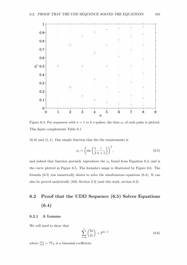
6.2. PROOF THAT THE UDD SEQUENCE SOLVES THE EQUATIONS 165
0 1 2 3 4 5 6 7 8 9
0
0.1
0.2
0.3
0.4
0.5
0.6
0.7
0.8
0.9
1
αi
n
Figure 6.4: For sequences with n = 1 to 8 π-pulses, the time αi of each pulse is plotted.
This figure complements Table 6.1.
(0, 0) and (1, 1). One simple function that fits the requirements is
αi =
(
sin
(
π
2
i
n + 1
))2
, (6.5)
and indeed that function precisely reproduces the αi found from Equation 6.4, and is
the curve plotted in Figure 6.5. The formula’s usage is illustrated by Figure 6.6. The
formula (6.5) was numerically shown to solve the simultaneous equations (6.4). It can
also be proved analytically [162, Section 2.3] (and this work, section 6.2).
6.2 Proof that the UDD Sequence (6.5) Solves Equations
(6.4)
6.2.1 A Lemma
We will need to show thatn∑
r=0
(
2n
2r
)
= 22n−1 (6.6)
where(
nk
)
= nCk is a binomial coefficient.

166 CHAPTER 6. DYNAMIC DECOUPLING
0 0.2 0.4 0.6 0.8 10
0.1
0.2
0.3
0.4
0.5
0.6
0.7
0.8
0.9
1
i/(n+1)
αi
1
2
3
4
5
6
7
8
Number n
of π Pulses
Figure 6.5: αi plotted against in+1 seems to lay all the points on the same curve. Equa-
tion (6.5) is shown as a dotted curve.
π
2π
2π
τ
πππ
104π
τ sin2( )
10π
τ sin2( )
103π
τ sin2( )
102π
τ sin2( )
Figure 6.6: A 4-pulse UDD spin-echo sequence whose timings are taken from Equation
(6.5).
It is well known that
(1 + x)m =
m∑
k=0
(
m
k
)
xk. (6.7)

6.2. PROOF THAT THE UDD SEQUENCE SOLVES THE EQUATIONS 167
Replacing m with 2n, and splitting odd and even terms we get
(1 + x)2n =2n∑
k=0
(
2n
k
)
xk (6.8)
=n∑
r=0
(
2n
2r
)
x2r +n−1∑
r=0
(
2n
2r + 1
)
x2r+1 (6.9)
Consider setting x to −1. Then
(1 + −1)2n =n∑
r=0
(
2n
2r
)
(−1)2r +n−1∑
r=0
(
2n
2r + 1
)
(−1)2r+1. (6.10)
0 =
n∑
r=0
(
2n
2r
)
−n−1∑
r=0
(
2n
2r + 1
)
(6.11)
so
n∑
r=0
(
2n
2r
)
=
n−1∑
r=0
(
2n
2r + 1
)
. (6.12)
Now consider setting x to 1. Then
22n =n∑
r=0
(
2n
2r
)
+n−1∑
r=0
(
2n
2r + 1
)
. (6.13)
But we have already shown that the two sums are equal, so
n∑
r=0
(
2n
2r
)
=n−1∑
r=0
(
2n
2r + 1
)
=1
222n (6.14)
= 22n−1 (6.15)
QED.
6.2.2 Useful Results
(sin(z))2n = 2−2n
(
2n
n
)
+ 21−2nn−1∑
k=0
(−1)n−k
(
2n
k
)
cos (2(n − k)z) n ∈ N+ (6.16)
n∑
k=0
(−1)k cos(ak) =cos(
12 (a + n(a + π))
)
cos(
n2 (a + π)
)
cos(
a2
) (6.17)
n∑
k=0
(−1)k sin(ak) =cos(
12 (a + n(a + π))
)
sin(
n2 (a + π)
)
cos(
a2
) (6.18)
These forms are from Wolfram Functions [163, 164, 165]. They can be derived using the
complex exponential forms of sine and cosine.
cos(A + B) = cos(A) cos(B) − sin(A) sin(B) (6.19)
is the standard cosine Double Angle Formula.

168 CHAPTER 6. DYNAMIC DECOUPLING
6.2.3 The Proof
We wish to prove that
(−1)n − 2n∑
i=1
(−1)iαji = 0 ∀j = 1, 2, . . . , n (6.20)
is solved by
αi =
(
sin
(
π
2
i
n + 1
))2
, (6.21)
which I shall do by proving the convenient rearrangement
U =n−1∑
I=0
(−1)I
(
sin
(
π
2
I + 1
n + 1
))2j
= −1
2(−1)n ∀j = 1, 2, . . . , n (6.22)
I present a direct, but longwinded, proof. A less direct but much shorter proof can be
found in Ref [162].
We start by expanding the power of sine in (6.22), using (6.16).
U =n−1∑
I=0
(−1)I
(
2
4j
j−1∑
m=0
(−1)j−m
(
2j
m
)
cos
(
π(j − m)I + 1
n + 1
)
+1
4j
(
2j
j
)
)(6.23)
Exchange the order of summation, and rearrange.
=(−1)j
4j
(
2
j−1∑
m=0
(−1)m
(
2j
m
) n−1∑
I=0
(−1)I cos
(
π(j − m)I + 1
n + 1
)
+ (−1)j
(
2j
j
) n−1∑
I=0
(−1)I
)(6.24)
=(−1)j
4j
(
2
j−1∑
m=0
(−1)m
(
2j
m
) n−1∑
I=0
(−1)I cos
(
π(j − m)I + 1
n + 1
)
+ (−1)j
(
2j
j
)
0 n even
1 n odd
)(6.25)
Use the cosine Double Angle Formula, to expand.
=(−1)j
4j
(
2
j−1∑
m=0
(−1)m
(
2j
m
) n−1∑
I=0
(−1)I
·(
cos
(
πj − m
n + 1
)
cos
(
πIj − m
n + 1
)
− sin
(
πj − m
n + 1
)
sin
(
πIj − m
n + 1
))
+ (−1)j
(
2j
j
)
0 n even
1 n odd
)
(6.26)

6.2. PROOF THAT THE UDD SEQUENCE SOLVES THE EQUATIONS 169
Use the summation formulae (6.17) and (6.18).
=(−1)j
4j
(
2
j−1∑
m=0
(−1)m
(
2j
m
)
·(
cos
(
πj − m
n + 1
)
cos
(
πn − 1
2
(
j − m
n + 1+ 1
)) cos(
π2
(
j−mn+1 + (n − 1)
(
j−mn+1 + 1
)))
cos(
π2
j−mn+1
)
− sin
(
πj − m
n + 1
)
sin
(
πn − 1
2
(
j − m
n + 1+ 1
)) cos(
π2
(
j−mn+1 + (n − 1)
(
j−mn+1 + 1
)))
cos(
π2
j−mn+1
)
)
+ (−1)j
(
2j
j
)
0 n even
1 n odd
)
(6.27)
Use the cosine Double Angle Formula again, but this time contracting.
=(−1)j
4j
(
2
j−1∑
m=0
(−1)m
(
2j
m
)
· cos
(
πn − 1
2
(
j − m
n + 1+ 1
)
+ πj − m
n + 1
) cos(
π2
(
j−mn+1 + (n − 1)
(
j−mn+1 + 1
)))
cos(
π2
j−mn+1
)
+ (−1)j
(
2j
j
)
0 n even
1 n odd
)
(6.28)
=(−1)j
4j
(
2
j−1∑
m=0
(−1)m
(
2j
m
)
·cos(
π2 (j − m + n − 1)
)
cos(
π2
(
j − m + n − 1 − j−mn+1
))
cos(
π2
j−mn+1
)
+ (−1)j
(
2j
j
)
0 n even
1 n odd
)
(6.29)
And one final use of a Double Angle Formula (in expansion).
=(−1)j
4j
(
2
j−1∑
m=0
(−1)m
(
2j
m
)
· cos(
π2 (j − m + n − 1)
)
cos(
π2
j−mn+1
)
(
cos(π
2(j − m + n − 1)
)
cos
(
π
2
j − m
n + 1
)
+ sin(π
2(j − m + n − 1)
)
sin
(
π
2
j − m
n + 1
))
+ (−1)j
(
2j
j
)
0 n even
1 n odd
)
(6.30)

170 CHAPTER 6. DYNAMIC DECOUPLING
Now, if j −m + n− 1 is odd, then sin(
π2 (j − m + n − 1)
)
= 0. But if j −m + n− 1
is even, then cos(
π2 (j − m + n − 1)
)
= 0 and the whole term vanishes. So
U =(−1)j
4j
(
2
j−1∑
m=0
(−1)m
(
2j
m
)
(
cos(π
2(j − m + n − 1)
))2
+ (−1)j
(
2j
j
)
0 n even
1 n odd
)(6.31)
Notice that when m = j,
cos(π
2(j − m + n − 1)
)
=
0 n even
1 n odd. (6.32)
So we can absorb the final term into the main summation, because(
nr
)
=(
nn−r
)
.
U =(−1)j
4j
2j∑
m=0
(−1)m
(
2j
m
)
(
cos(π
2(j − m + n − 1)
))2(6.33)
=(−1)j
4j
2j∑
m=0
(−1)m
(
2j
m
)
0 j − m + n even
1 j − m + n odd(6.34)
=−(−1)j(−1)j+n
4j
2j∑
m=0
(
2j
m
)
0 j − m + n even
1 j − m + n odd(6.35)
=−(−1)n
4j
∑jk=0
(
2j2k
)
j + n odd∑j−1
k=0
(
2j2k+1
)
j + n even(6.36)
Use (6.15)
=−(−1)n
4j× 1
24j (6.37)
U = −1
2(−1)n (6.38)
QED.
6.2.4 Optimality
I have not formally proved that the UDD pulse sequence is optimal – i.e. I have not
proved that to cancel out an (n − 1)th order polynomial requires n pulses; only that n
are sufficient. However, the following argument suggests that n pulses are necessary in
general.
The polynomial is described by n real numbers pj that must be independently can-
celled by the sequence. So all n of the equations (6.4) are needed. To solve n simultane-

6.3. THE LITERATURE 171
ous equations generally requires one to solve for n variables. Here, these are the times
of the n pulses; so n pulses are required.
It seems likely that the UDD sequence is the only solution to the equations, and
hence is optimal for cancelling magnetic field drifts in the polynomial model.
6.3 The Literature
6.3.1 Theory
The pulse sequence defined by (6.5), and illustrated in Figure 6.6, had been previously
discovered by Gotz S. Uhrig [166]. He derived it in the context of a qubit that interacts
with a bath of bosons via the Hamiltonian
H =∑
i
ωib†ibi +
1
2σz
∑
i
λi
(
b†i + bi
)
+ E (6.39)
where λi and ωi are properties of the bath that define its spectral density; b(†)i are
(creation) annihilation operators for quanta in the bath; E is an energy offset; and
σz is a Pauli spin operator acting on the qubit (assumed to be a spin-half particle).
The sequence was found to provide optimal protection from decoherence in that model,
and numerical simulations showed that it outperformed the standard CPMG sequence
(6.40, below). The detailed derivation [162] treats a sequence of π-pulses as a filter in
the frequency domain. Uhrig demands that the first n derivatives of the filter function
vanish in the low frequency limit, which leads to Equations (6.4). The general technique
of using a sequence of pulses to protect a qubit (which originated in the field of Nuclear
Magnetic Resonance) is called Dynamical Decoupling (DD); the sequence of Equation
(6.5) has become known as Uhrig DD (UDD).
Since this first appearance in the literature, UDD has been shown to have other re-
markable properties. Lee, Witzel and Das Sarma [167] showed that UDD is the optimal
decoupling process for any dephasing Hamiltonian, provided that τ is short compared
to the timescale of the noise. They claim that, with each added pulse, UDD cancels
out successive powers of τ in the decoherence of the spin-echo signal. However, their
chosen formalism (expanding the time evolution operator as a double sum of products
of Hamiltonians) leads to a set of simultaneous nonlinear equations that grows exponen-
tially with n – as opposed to the linearly growing set in [162] and this work. They are
therefore able to algebraically prove the claim only for n ≤ 9, with numerical “proof”
172 CHAPTER 6. DYNAMIC DECOUPLING
for n ≤ 14. Similarly, Dhar et al. [168] had earlier derived UDD sequences for n ≤ 4 but
did not find the general formula (although their 5-pulse sequence disagrees with UDD).
Other authors [169, 141, 170] continue with the treatment of UDD as a filter.
Cywinski in particular [169] lists the filter functions of a variety of DD pulse sequences,
and shows numerically and algebraically that UDD is by far the best in the limit ωτ ≪ n.
Biercuk et al. [170] derive the filter function for UDD where the π-pulses have non-zero
length (rather than being idealised δ-functions).
However, for longer times τ or higher noise frequencies, UDD is not the best [169]. In
particular it is overtaken by the simpler Carr-Purcell-Meiboom-Gill (CPMG) sequence,
in which the π-pulse times are given by
αi =12 + i − 1
n(6.40)
for i = 1, . . . , n. See also Figure 6.7. CPMG has been used for many years in NMR
experiments [171], although not usually in the context of a quantum memory. The
Meiboom-Gill contribution to CPMG is that each π-pulse has a phase shift of π2 (or −π
2 ,
although it should be the same for each pulse) relative to the π2 -pulses. The sequence
can be described as 90x, 180y, 180y, . . . , 90x where the subscript indicates the axis of
rotation in the Bloch sphere. This does not improve the noise-filtering properties of the
sequence, but it prevents imperfections in the π-pulses from accumulating. This may
be useful to improve the contrast in our experiments (without biasing the measurement
of the coherence time). But it probably won’t help in practical usage of the sequence –
in a quantum computer we want to be able to dynamically decouple any initial qubit
state, not just (|0〉 − i |1〉) /√
2 that is prepared here, and in the general situation the
Meiboom-Gill phase shift gives no benefit on average.
6.3.2 Experiment
Biercuk et al. have provided the only experimental implementation of UDD so far
[141, 170, 172]. They used a 4.5 T superconducting-magnet Penning trap and an
ensemble of ∼ 1000 9Be+ ions, with qubit states in S1/2 (|mI = 3/2, mJ = 1/2〉 and
|mI = 3/2, mJ = −1/2〉). The qubit splitting is ≈ 124 GHz with field sensitivity
≈ 28 MHz/mT, and they achieve π times of ≈ 185 µs.
In Ref [170] they show (in simulation and experiment) that UDD is much more
robust than CPMG against detuned or wrong-length pulses. They also experimented

6.3. THE LITERATURE 173
π
2π
2π
τ
πππ
83τ
85τ
87τ
8τ
4τ
4τ
4τ
8τ
Figure 6.7: A 4-pulse CPMG spin-echo sequence whose timings are taken from Equation
6.40.
with injecting magnetic field noise with various power spectra. When they injected noise
whose power spectrum is proportional to frequency (S(ω) ∝ ω), UDD maintained high
phase coherence for much longer than CPMG. However, they also tried noise with power
inversely proportional to frequency (S(ω) ∝ ω−1) – although UDD still won at short
times, the coherence fell sharply while CPMG was still maintaining some coherence.
With their ambient noise (power spectrum S(ω) ∝ ω−4) CPMG is almost as good as
(or better than) UDD for most times, to within the experimental precision.
In a later paper, they show [141] that pulse sequences can be optimised for any
given, specific noise spectrum that may exist in some experiment. Such a sequence
can outperform both CPMG and UDD, even in the high-fidelity (low noise/short time)
regime where UDD is more generally optimal. They are able to perform the optimisation
experimentally, where at each step of the algorithm the proposed sequence is applied to
the ions and the coherence measured.
In fact, their third paper [172] makes such optimisation much simpler. They use
numerical modelling to minimise the integral of an n-pulse sequence’s filter function
over some range of frequencies [0, ωc], where ωc is some high-frequency cut-off of the
noise spectrum. Note that only the filter is involved in this optimisation – the noise is
still unknown. The optimum sequence depends on τ ′ ≡ ωcτ , a spectrum-independent
measure of the total sequence time. UDD is taken as the inital guess at τ ′ = 0, and
the sequence diverges away from it as τ ′ increases. Having calculated a large number
of sequences, for a variety of values of τ ′, they start their experiment. As before, they
do an optimisation procedure using the experimental results as the feedback. But this
time, the sequences are selected only from the pre-calculated set, optimising in just
174 CHAPTER 6. DYNAMIC DECOUPLING
one dimension (τ ′). This is far easier than the n-dimensional task of optimising each
pulse location individually. Once the sequence has been selected, it is simply scaled
uniformly to match the desired qubit storage time. Surprisingly the procedure is shown
(in simulation) to perform very nearly as well as full optimisation, outperforming the
fixed sequences UDD and CPMG. Their experiment also shows it preserving coherence
better than CPMG and UDD for synthesised noise. However, it is worse for their ambient
magnetic field noise that does not have a sharp high-frequency cutoff.
6.4 Our Experiment
6.4.1 AC Field Compensation
I have used our hyperfine 43Ca+ stretch-state qubit to verify that UDD (and CPMG)
are highly effective at lengthening the coherence time of a single ion qubit. Our group
has already measured the coherence time of a clock-state qubit to be T2 = 1.2(2) s [58];
if a single spin-echo pulse were used, no decoherence was detectable (at the 1% level)
in a 1 second Ramsey gap. It would thus be intolerably slow to use clock states in
this experiment, combined with the fact that we can only prepare those states with
probability ∼ 17 .
An initial worry was that the qubit frequency varies with time due to the 50 Hz
mains. Ben Keitch [97] found that the frequency varied by ≈ 10 kHz pk-pk over a whole
AC cycle. We can drive the qubit at a Rabi frequency of up to 18 kHz; a 10 kHz detuning
would thus significantly degrade the fidelity of a π-pulse. Increasing the power of the
microwaves is the obvious solution, but more powerful amplifiers at GHz frequencies
are expensive. We currently use a Minicircuits ZVE-8G that puts out nearly 29 dBm ≈
750 mW (nominally 33 dBm ≈ 1.8 W at the 1 dB compression point) and costs more
than $1000. The ZVE-3W-83 costs $200 more for an extra 1 dB – a factor of 1.26. Since
the Rabi frequency is proportional to the amplitude of the oscillating magnetic field
at the ion, which is proportional to the square root of the radiated microwave power,
the Rabi frequency would rise by only 12%. A 20 W amplifier would increase the Rabi
frequency by a factor of 5, at a cost of ≈ £1500.
Keitch attempted to use a Spicer SC-20 field-cancelling system [97]. This is a com-
mercial system that measures the magnetic field with two sensors, each measuring the
field along three perpendicular axes. It uses a feedback circuit to try to keep the field be-

6.4. OUR EXPERIMENT 175
tween the sensors constant by sending current through three large, perpendicular coils.
The user can adjust the gain of the feedback loop and the relative weighting of each
sensor separately for each axis. But although he tried a wide variety of settings, the
unit was unable to reliably cancel out field fluctations, including the 50 Hz mains.
The AC line field should be easy to cancel because it is regular and stable. One idea
is to use a line-locked 50 Hz signal to frequency-modulate the microwave synthesizer (on
an analogue channel). The microwaves would thus follow the ion’s frequency, and the
base microwave frequency could still be set by communication with the computer via the
RS-232 serial port. However, we must also be able to use analogue phase modulation
so that we can alter the phase of the final π2 -pulse in Ramsey experiments, and our
synthesisers do not allow frequency and phase modulation at the same time.
Instead, I installed a 20-turn coil to allow a deliberate 50 Hz field to be driven to
oppose the AC line field. A 10(2) µF capacitor is connected in parallel with the coil,
as a crude low-pass filter. The coil’s resistance is 0.135(5) Ω (from a four-terminal
measurement) so the approximate cutoff frequency of the filter is 12πRC = 120(20) kHz.
The coil is placed with its axis parallel to the fixed magnetic field (which is parallel
with the σ-polarised beams), close to the window through which R‖ enters the vacuum
system (see Figure 2.5).
First I tried to drive the coil directly from the mains (with step-down transformers
including a variable one), but this leads to the “correction” field being out of phase
with the ambient field, and the phase is not adjustable. The eventual solution was to
drive the coil with a signal generator (Stanford Research Systems DS345). We could,
of course, use a phase-locked-loop to keep the signal synchronised with the mains, but
instead I choose a simpler method.
The Stanford has a mode in which it emits a burst (an integer number of periods) of
signal in response to some trigger, and then waits for the next trigger. While it waits, the
output voltage is held constant at its value at the end of the burst. The trigger options
include triggering from the mains. This gives us a 50 Hz signal that accurately follows
the mains, provided that one can be sure that the Stanford finishes its cycle before
the next trigger (otherwise it misses the next cycle completely). We must therefore set
the signal frequency to just over 50 Hz: 50.2 Hz seems to work well with the following
settings.
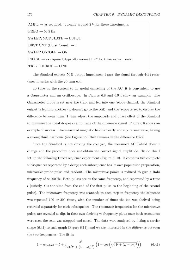
176 CHAPTER 6. DYNAMIC DECOUPLING
AMPL → as required, typically around 2 V for these experiments.
FREQ → 50.2 Hz
SWEEP/MODULATE → BURST
BRST CNT (Burst Count) → 1
SWEEP ON/OFF → ON
PHASE → as required, typically around 100 for these experiments.
TRIG SOURCE → LINE
The Stanford expects 50 Ω output impedance; I pass the signal through 44 Ω resis-
tance in series with the 20-turn coil.
To tune up the system to do useful cancelling of the AC, it is convenient to use
a Gaussmeter and an oscilloscope. In Figures 6.8 and 6.9 I show an example. The
Gaussmeter probe is set near the trap, and fed into one ’scope channel; the Stanford
output is fed into another (it doesn’t go to the coil); and the ’scope is set to display the
difference between them. I then adjust the amplitude and phase offset of the Stanford
to minimise the (peak-to-peak) amplitude of the difference signal. Figure 6.8 shows an
example of success. The measured magnetic field is clearly not a pure sine wave, having
a strong third harmonic (see Figure 6.9) that remains in the difference trace.
Since the Stanford is not driving the coil yet, the measured AC B-field doesn’t
change and the procedure does not obtain the correct signal amplitude. To do this I
set up the following timed sequence experiment (Figure 6.10). It contains two complete
subsequences separated by a delay; each subsequence has its own population preparation,
microwave probe pulse and readout. The microwave power is reduced to give a Rabi
frequency of ≈ 960 Hz. Both pulses are at the same frequency, and separated by a time
t (strictly, t is the time from the end of the first pulse to the beginning of the second
pulse). The microwave frequency was scanned; at each step in frequency the sequence
was repeated 100 or 200 times, with the number of times the ion was shelved being
recorded separately for each subsequence. The resonance frequencies for the microwave
pulses are revealed as dips in their own shelving vs frequency plots; once both resonances
were seen the scan was stopped and saved. The data were analysed by fitting a carrier
shape (6.41) to each graph (Figure 6.11), and we are interested in the difference between
the two frequencies. The fit is:
1 − nShelved = b + aΩ2
2 (Ω2 + (ω − ω0)2)
(
1 − cos(
√
Ω2 + (ω − ω0)2))
(6.41)
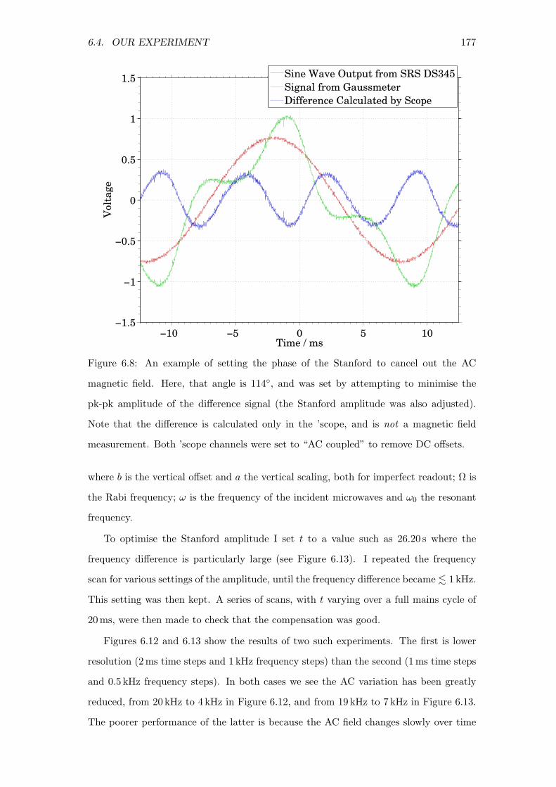
6.4. OUR EXPERIMENT 177
−10 −5 0 5 10−1.5
−1
−0.5
0
0.5
1
1.5
Time / ms
Volt
age
Sine Wave Output from SRS DS345
Signal from Gaussmeter
Difference Calculated by Scope
Figure 6.8: An example of setting the phase of the Stanford to cancel out the AC
magnetic field. Here, that angle is 114, and was set by attempting to minimise the
pk-pk amplitude of the difference signal (the Stanford amplitude was also adjusted).
Note that the difference is calculated only in the ’scope, and is not a magnetic field
measurement. Both ’scope channels were set to “AC coupled” to remove DC offsets.
where b is the vertical offset and a the vertical scaling, both for imperfect readout; Ω is
the Rabi frequency; ω is the frequency of the incident microwaves and ω0 the resonant
frequency.
To optimise the Stanford amplitude I set t to a value such as 26.20 s where the
frequency difference is particularly large (see Figure 6.13). I repeated the frequency
scan for various settings of the amplitude, until the frequency difference became . 1 kHz.
This setting was then kept. A series of scans, with t varying over a full mains cycle of
20 ms, were then made to check that the compensation was good.
Figures 6.12 and 6.13 show the results of two such experiments. The first is lower
resolution (2 ms time steps and 1 kHz frequency steps) than the second (1 ms time steps
and 0.5 kHz frequency steps). In both cases we see the AC variation has been greatly
reduced, from 20 kHz to 4 kHz in Figure 6.12, and from 19 kHz to 7 kHz in Figure 6.13.
The poorer performance of the latter is because the AC field changes slowly over time

178 CHAPTER 6. DYNAMIC DECOUPLING
−0.05 −0.04 −0.03 −0.02 −0.01 0 0.01 0.02 0.03 0.04 0.05
0
Time / s
Ma
gn
eti
c F
ield
/
Arb
itra
ry U
nit
s
0 50 150 250 350 450 550 650 750 850 950 1050 1150 125010
−3
10−2
10−1
100
101
102
Frequency / Hz
Am
pli
tud
e /
Arb
itra
ry U
nit
s
Figure 6.9: [Top] A 0.1 s sample of the AC line field, as measured by the Gaussmeter.
Arbitrary vertical units. [Bottom] Fourier Transform of the AC line field measured by
Gaussmeter; from a 1 s sample.
(for instance, if mains-powered devices are switched on or off), and the scan was done
seven days after setting the phase and amplitude. Notice also that, while the uncancelled
data does not perfectly resemble the Gaussmeter-measured field in Figure 6.8, there is
a third harmonic residual clearly visible in the field-cancelled data. The Stanford is also
an arbitrary waveform generator, so it would probably be possible to cancel that and
other hamonics if necessary.
A π-pulse with Rabi frequency 2π × 18 kHz, assumed to have perfect fidelity at zero
detuning, has 95% fidelity at a detuning of 4 kHz; 82% at 8 kHz; and only 23% at 20 kHz.
These are the respective approximate worst case fidelities of π-pulses with the coil well-
tuned (Figure 6.12), with the coil imperfectly tuned (Figure 6.13) and with no coil in
use. Without using the coil, some π-pulses would have extremely low fidelities and the
experiment would be impossible.

6.4. OUR EXPERIMENT 179
Figure 6.10: The sequence of pulses used to measure how the ion’s microwave resonance
frequency varies due to the magnetic field due to AC mains currents. The sequence is
triggered to always start at the same point in the mains cycle.
6.4.2 Spin-Echo Sequences
To implement DD sequences (mostly Uhrig, but also CPMG for comparison), I inserted
an appropriately-timed series of π-pulses in the gap of a Ramsey experiment. The qubit
was initially prepared in (|0〉 − i |1〉) /√
2 by a π2 -pulse, left for a delay τ (including
the refocussing π-pulses, if any), and measured with a second π2 -pulse. The phase
of the second pulse was scanned, using the analogue phase modulation control of the
Agilent synths and a DAC channel. The fringes obtained were fit by a sine function,
whose frequency was constrained to ±15% of the average frequency obtained from an
unconstrained fit. We are only interested in the amplitude of that sine, which is the
contrast of the fringes and is plotted in the graphs.
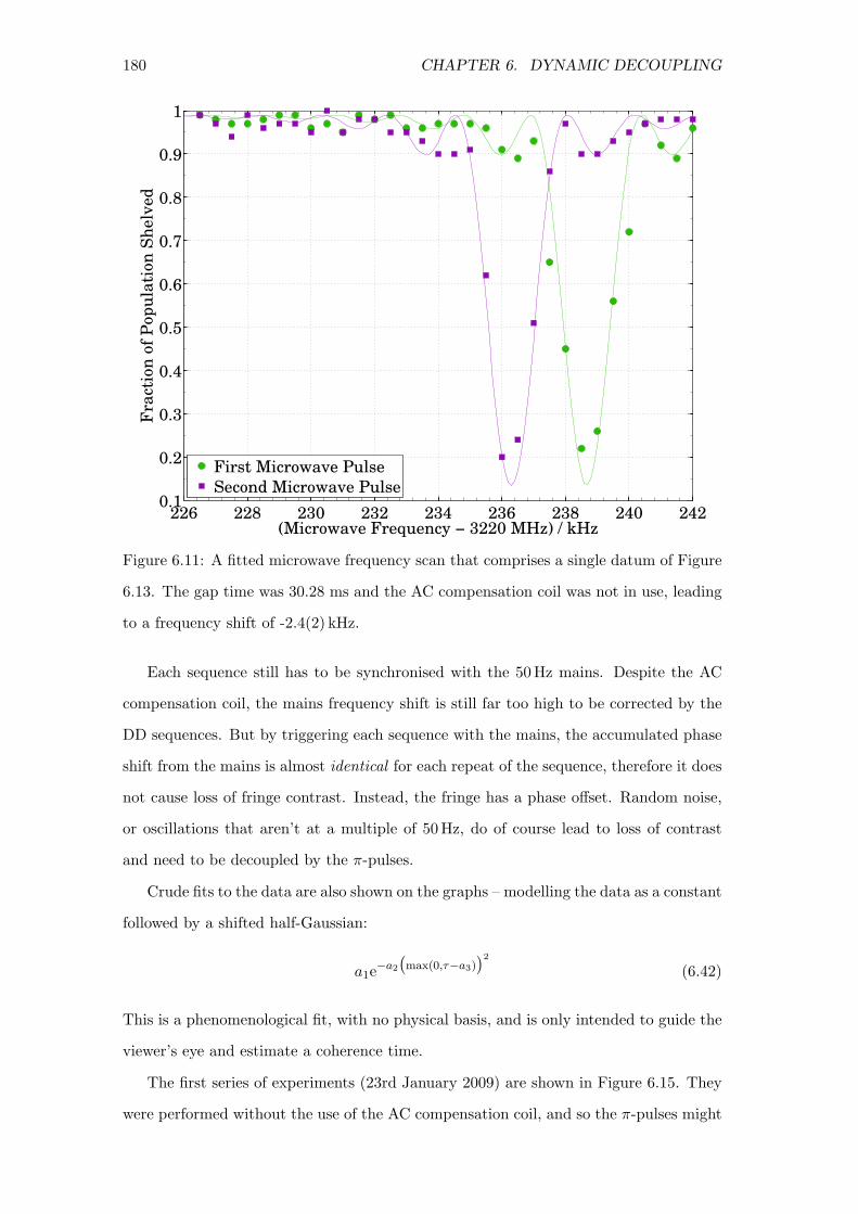
180 CHAPTER 6. DYNAMIC DECOUPLING
226 228 230 232 234 236 238 240 2420.1
0.2
0.3
0.4
0.5
0.6
0.7
0.8
0.9
1
(Microwave Frequency − 3220 MHz) / kHz
Fra
ctio
n o
f P
op
ula
tion
Sh
elv
ed
First Microwave Pulse
Second Microwave Pulse
Figure 6.11: A fitted microwave frequency scan that comprises a single datum of Figure
6.13. The gap time was 30.28 ms and the AC compensation coil was not in use, leading
to a frequency shift of -2.4(2) kHz.
Each sequence still has to be synchronised with the 50 Hz mains. Despite the AC
compensation coil, the mains frequency shift is still far too high to be corrected by the
DD sequences. But by triggering each sequence with the mains, the accumulated phase
shift from the mains is almost identical for each repeat of the sequence, therefore it does
not cause loss of fringe contrast. Instead, the fringe has a phase offset. Random noise,
or oscillations that aren’t at a multiple of 50 Hz, do of course lead to loss of contrast
and need to be decoupled by the π-pulses.
Crude fits to the data are also shown on the graphs – modelling the data as a constant
followed by a shifted half-Gaussian:
a1e−a2
(
max(0,τ−a3))2
(6.42)
This is a phenomenological fit, with no physical basis, and is only intended to guide the
viewer’s eye and estimate a coherence time.
The first series of experiments (23rd January 2009) are shown in Figure 6.15. They
were performed without the use of the AC compensation coil, and so the π-pulses might

6.4. OUR EXPERIMENT 181
0 5 10 15 20 25−4
−2
0
2
4
6
8
10
12
14
16
Gap Time / ms
Fre
qu
en
cy S
hif
t /
kH
z
Coil used
Coil not used
Figure 6.12: Comparison of the shift in the qubit frequency due to the 50 Hz mains,
with and without the compensation coil. The Stanford’s phase and amplitude had just
been adjusted.
have very low fidelity at certain times in the AC mains cycle.
The second set of experiments (6th March 2009) used the AC compensation coil,
which allowed me to use long sequences with confidence that the π-pulses would remain
at high fidelity. Sometimes, when a scan gave a poorer contrast than expected for the
delay time, I would check the microwave resonant frequency and find it had shifted,
requiring the DD scan to be repeated. I also started using the Meiboom-Gill phase shift
for the π-pulses, because preliminary experiments implied a small improvement (but see
Figure 6.17).
The third set of experiments (12th and 13th March 2009) used the compensation
coil, and to maintain a constant, high fidelity for the π-pulses I checked and set the
microwave frequency before every scan. This set included the data of Figure 6.16, which
used CPMG and UDD sequences with the same number of π-pulses.
The fourth set of experiments (16th and 17th April 2009) included five-pulse se-
quences perfomed with and without the Meiboom-Gill phase shift. This is essen-
tially equivalent to testing the Uhrig sequence for both |R〉 = (|0〉 − i |1〉) /√
2 and
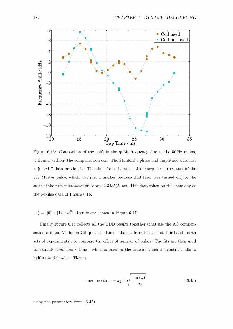
182 CHAPTER 6. DYNAMIC DECOUPLING
10 15 20 25 30 35−12
−10
−8
−6
−4
−2
0
2
4
6
8
Gap Time / ms
Fre
qu
en
cy S
hif
t /
kH
z
Coil used
Coil not used
Figure 6.13: Comparison of the shift in the qubit frequency due to the 50 Hz mains,
with and without the compensation coil. The Stanford’s phase and amplitude were last
adjusted 7 days previously. The time from the start of the sequence (the start of the
397 Master pulse, which was just a marker because that laser was turned off) to the
start of the first microwave pulse was 2.3485(5) ms. This data taken on the same day as
the 6-pulse data of Figure 6.16.
|+〉 = (|0〉 + |1〉) /√
2. Results are shown in Figure 6.17.
Finally Figure 6.18 collects all the UDD results together (that use the AC compen-
sation coil and Meiboom-Gill phase shifting – that is, from the second, third and fourth
sets of experiments), to compare the effect of number of pulses. The fits are then used
to estimate a coherence time – which is taken as the time at which the contrast falls to
half its initial value. That is,
coherence time = a3 +
√
− ln(
12
)
a2(6.43)
using the parameters from (6.42).

6.4. OUR EXPERIMENT 183
Figure 6.14: A 20-pulse Uhrig sequence. This one has 40 ms between the two π2 -pulses.
6.4.2.1 Conclusions
All the experiments show that dynamic decoupling is extremely effective at prolonging
the phase coherence of the qubit. In a basic Ramsey experiment with no π-pulses, the
contrast stays above half its initial value for ≈ 0.45 ms. With just a single π-pulse,
the standard spin-echo sequence increases this to ≈ 2 ms. Six pulses keep coherence
for ≈ 12 ms, and twenty pulses, ≈ 28 ms. Notice also that the contrast does not decay
exponentially; instead it seems to fall linearly with time, or even have a plateau of high
contrast at short delays and then a sharp drop. This tells us that the noise in our
trap is highly correlated over these timescales; Cywinski [169, Section III] says that
signal ∝ e− τ
T2 only occurs when the noise autocorrelation time is much smaller than T2.
One more thing to notice from Figure 6.18 is that the results are reliably similar from
day to day.

184 CHAPTER 6. DYNAMIC DECOUPLING
0 1 2 3 4 5 6 7 80
0.1
0.2
0.3
0.4
0.5
0.6
0.7
0.8
0.9
1
τ / ms
Fri
nge C
on
tra
st (
not
norm
ali
sed
)
0
1
2
3
No. of π pulses
Figure 6.15: UDD sequences with from zero to three π-pulses. AC compensation coil is
not used.
The amplitude of the magnetic field noise can be estimated, even though we have
been unable to calculate it precisely from detailed simulations and fits to the data1.
Consider, for instance, the n = 0 Ramsey experiments. The coherence vanished for
τ & 0.8 ms, so in 0.8 ms the spurious accumulated phase was ∼ π and the angular
frequency error was δ ≈ π/τ ≈ 4 kHz. This corresponds to a magnetic field of ≈ 1.5 mG.
The sequence was repeated identically 200 times for each point of the Ramsey fringe,
taking 4 s for each point, and it is the change in magnetic field over this timescale that
gives measurable dephasing. So we see that the magnetic field fluctuation at the 4 s
timescale is ≈ 1.5 mG.
The average fidelity of each π-pulse is approximately 98% for n = 3 to 20 pulses,
which is what we may expect given the residual field variations of Figures 6.12 and 6.13.
Figure 6.16 shows that the CPMG sequence is just as good, if not better, at main-
taining fringe contrast as UDD. This matches the findings of Cywinski [169] in the long
time or high noise regime.
1An example of such a calculation is from [169], but it requires measurements with large n and small
τ that we are currently unable to perform

6.4. OUR EXPERIMENT 185
0 5 10 15 20 25 30 35 40 450
0.1
0.2
0.3
0.4
0.5
0.6
0.7
0.8
0.9
1
τ / ms
Fri
nge C
on
tra
st (
not
norm
ali
sed
)
20 [Uhrig]
20 [CPMG]
6 [Uhrig]
6 [CPMG]
No. of π pulses
Figure 6.16: Comparing UDD and CPMG sequences for six and twenty π-pulses. Hollow
symbols are anomalous data points excluded from the fits. AC compensation coil in use.
Unfortunately I have not been able to test the sequences’ effectiveness in the short
time regime. This is partly because the large variability in the fringe contrasts I measured
would obscure any subtle variability due to real effects; and partly because our finite π
time imposes a minimum τ that can be tested for a given number of pulses. To speed
up the experiments, it would be desirable to emulate Biercuk et al. [141, 170] and not
do a phase scan at all. They scanned only the delay time, and simply recorded the
probability of shelving after the final π2 -pulse. Unfortunately that may not be practical
for us; our fringes also have different phase offsets for different Ramsey delays. This is
probably due to the residual AC mains field, which is constant for every experimental
run and hence does not reduce the fringe contrast, but could give the qubit a phase
shift that varies with the delay time. The Biercuk method would confuse this for loss of
phase contrast.
Figure 6.17 shows data with and without the Meiboom-Gill phase shift. Preliminary
experiments suggested that the Meiboom-Gill phase shift improves the initial contrast,
although it was not expected to affect the decoherence time. In fact, it seems to make
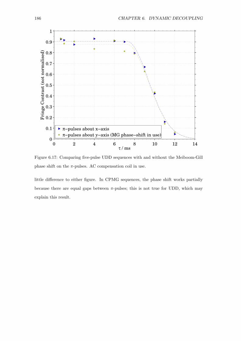
186 CHAPTER 6. DYNAMIC DECOUPLING
0 2 4 6 8 10 12 140
0.1
0.2
0.3
0.4
0.5
0.6
0.7
0.8
0.9
1
τ / ms
Fri
nge C
on
tra
st (
not
norm
ali
sed
)
π−pulses about x−axis
π−pulses about y−axis (MG phase−shift in use)
Figure 6.17: Comparing five-pulse UDD sequences with and without the Meiboom-Gill
phase shift on the π-pulses. AC compensation coil in use.
little difference to either figure. In CPMG sequences, the phase shift works partially
because there are equal gaps between π-pulses; this is not true for UDD, which may
explain this result.

6.4. OUR EXPERIMENT 187
0 5 10 15 20 25 30 35 40 450
0.1
0.2
0.3
0.4
0.5
0.6
0.7
0.8
0.9
1
τ / ms
Fri
nge C
on
tra
st (
not
norm
ali
sed
)
0
1
1
3
5
6
6
6
10
20
20
No. of π pulses
0 2 4 6 8 10 12 14 160
0.1
0.2
0.3
0.4
0.5
0.6
0.7
0.8
0.9
1
τ / ms
Fri
nge C
on
tra
st (
not
norm
ali
sed
)
0
1
1
3
5
6
6
6
No. of π pulses
Figure 6.18: Comparing UDD sequences with from 0 to 20 π-pulses [top] or 0 to 6
π-pulses [bottom]. The different symbols denote the number of π-pulses used for that
sequence; different colours for the same symbol indicate data from different days. Hollow
symbols are anomalous data points excluded from the fits. AC compensation coil in use.

188 CHAPTER 6. DYNAMIC DECOUPLING
0 5 10 15 200
5
10
15
20
25
30
35
Number of π−Pulses
Coh
ere
nce
Tim
e /
ms
Linear fit, 0−10 pulses
Linear fit, 0−20 pulses
Figure 6.19: The coherence time, as measured by (6.43), is plotted against the number
of UDD π-pulses. A straight line provides a reasonable fit to the data, especially if the
point at 20 pulses is excluded from the fit.

Chapter 7
Conclusion
This thesis described work concerned with detection and protection of quantum bits,
focussing on trapped ions and 43Ca+ in particular.
The first stage was to develop a full rate equations model of the states and transitions
of a 43Ca+ ion. It includes the 4S, 4P and 3D levels and automatically calculates
hyperfine structure. While such simulations do not include coherent effects such as dark
resonances, and thus disagree with experimental data in some circumstances, they are
accurate enough to predict and explain the results of experiments with far off-resonant
laser beams. This is relevant for readout and sympathetic cooling.
The speed of rate-equations simulations allows them to be used to optimise an
electron-shelving readout method in 43Ca+. The procedure uses pulses of tuned, σ+
polarised 393 nm light to transfer ions from S41/2 to D5/2, while causing as few transfers
as possible from S31/2. Approximately 10% of the time, the ion is transferred to D3/2
instead; the procedure repumps back to S41/2 with pulses of 850 nm light, carefully tuned
and polarised to minimise unwanted transfer to S31/2. The predicted maximum fidelity
of the process was 99.968% at a time of 100 µs. Restricting the time to 10 µs allows
99.958% fidelity.
The shelving method could be simplified while retaining high fidelity by using a
single pulse in which all three laser beams (393σ+, 850σ+, 850π) are switched on. This
achieves up to 99.965% fidelity, but is significantly slower than the multipulse method.
Even simpler, a single circularly-polarised 850 nm beam at a small angle (∼ 2) to the
magnetic field direction achieves up to 99.963% fidelity in 300 µs. The shelving was
shown to be robust against errors of pulse timing, laser intensity and beam polarisation.
Experimentally, a readout fidelity of up to 99.77(4)% was performed, including all
189
190 CHAPTER 7. CONCLUSION
error sources. We remove the measured error due to fluorescence detection (0.097(17)%)
to obtain the fidelity for shelving alone: F = 99.87(2)% in 400 µs. Despite the method’s
predicted robustness, this is an error five times larger than the theoretical optimum –
possibly due to setting the 393 intensity twice as high as is ideal, and having 0.13% σ−
impurity in the 850 beam.
Experiments were performed with a mixed pair of ions, 40Ca+ and 43Ca+. In contrast
with the pure 40Ca+ case, we discovered high heating and motional decoherence rates, as
well as frequent decrystallisation and other problems. This prevented us from reaching
our aim – an entangling phase gate between the two isotopes. As I describe below, we
will soon make several major improvements to the apparatus. We decided it would not
be efficient to spend any more time tracking down the problems, since the trap would
soon be replaced anyway.
Dephasing of qubits is a major source of errors in quantum information processing. A
spin-echo pulse sequence was derived that can eliminate phase errors when the dephasing
is caused by a frequency drift that is an arbitrary polynomial in time. If its highest-order
term is tn−1, then n π-pulses are required and should be spaced at times
τ sin2(
π2
1n+1
)
, τ sin2(
π2
2n+1
)
, . . . , τ sin2(
π2
nn+1
)
where the qubit’s original state is recovered at t = τ . The derived sequence is the same
as the one that had previously been derived by Uhrig, by treating the sequence as a filter
function; I have reviewed the relevant literature on this dynamical decoupling method.
The sequence was implemented on a single trapped 43Ca+ ion. But first, to improve
the π-pulse fidelity, a coil was installed to cancel out the (50 Hz component of the)
magnetic field of the mains. The sequence was then tested. Using 0, 1, 3, 5, 6, 10 and
20 π-pulses gave coherence times of, respectively, 0.4 ms, 1.9 ms, 5.7 ms, 9.8 ms, 12 ms,
18 ms and 30 ms. Twenty pulses gave a 75-fold enhancement, using the ambient noise
environment of our experiment. The simpler CPMG pulse sequence was equally effective,
which suggests that our ambient noise is outside the low-frequency regime where UDD
would be optimal. We saw no significant change between performing π-pulses about the
x or y-axes.

7.1. FUTURE DEVELOPMENTS 191
7.1 Future Developments
We have begun constructing a new trap and vacuum chamber, with several benefits
over the current apparatus. The trap will be a linear Paul trap like our current one,
but ≈ 40% of the size (ion-electrode distance = 0.5 mm). We hope to reach secular
frequencies up to ωr = 2π × 3.6 MHz and ωz = 2π × 2 MHz. The vacuum chamber
will be based on an octagon rather than the current hexagon – this will allow laser
access both parallel and perpendicular to the magnetic field, so that π-polarised light is
available for optical pumping into clock states, or testing the faster shelving methods.
The new trap’s higher secular frequency will make ground-state cooling significantly
easier than it is currently, because the Doppler limit will then be nz ≈ 2. We should be
able to omit the slow continuous sideband cooling step in motional experiments. We will
be able to use higher aspect ratios (much stronger radial than axial potential), without
reducing axial frequency, compared with in our current trap, which should improve the
crystallisation of 40-43 pairs. We will be able to make a better study of mixed crystals
than described in this work, and aim to implement the mixed-species quantum logic gate
and use it for a classical AND gate. Furthermore, we have recently purchased a pair
of Toptica TA-SHG110 lasers producing 130 mW at 397 nm for use as a Raman laser
with 43Ca+. Higher Raman beam intensities allow the beams to be further detuned for
a given Rabi frequency, reducing gate decoherence due to photon scattering.
The chamber and trap electrodes will be made out of 316 stainless steel, which
is less magnetisable than standard stainless steel; we expect this to reduce the stray
magnetic fields at the ion. Two coaxial feedthroughs will be included for more efficient
transfer of microwave signals to the ion. The feedthroughs will be connected inside the
chamber, allowing microwaves both in and out (passing the ion on the way): this gives
us the flexibility to terminate the transmission line with a 50 Ω absorber, a reflective
open/closed circuit or some other terminator, whichever turns out to give the highest
Rabi frequency.
Even though multi-well microtraps will become increasingly important in the future
for demonstrating the scalablity of ion-trap quantum computing, a simple, low-heating-
rate trap such as this will remain useful for many interesting experiments.

192 CHAPTER 7. CONCLUSION

Appendix A
Hyperfine Structure of 43Ca+
The following graphs show the hyperfine structure of the transitions of 43Ca+. Each
hyperfine component is drawn as a thick black solid vertical line. Its x-position indi-
cates the frequency of the component, and the height shows the branching ratio of that
component. The branching ratio from an upper state j to a lower state i is given by:
Brj→i =Γj→i
∑
k Γj→k=
Γj→i
Γj(A.1)
where Γj→i is the spontaneous transition rate from j to i, and Γj is the total decay
rate out of j to any level. The branching ratio also indicates the strength of stimulated
transitions between i and j (see Section 3.1.2.1).
Each hyperfine component is labeled as Fj → Fi (upper to lower). Also shown for
397 nm and 393 nm are the positions of the 40Ca+ resonance, as a dotted line (the height
of this line is not significant). Note that the 850 nm component P33/2 → D3
3/2 is forbidden.
193

194 APPENDIX A. HYPERFINE STRUCTURE OF 43CA+
−2500 −2000 −1500 −1000 −500 0 500 1000 1500 20000
0.1
0.2
0.3
0.4
0.5
0.6
0.7
0.8
Frequency detuning in MHz relative to the centre of gravity
Bra
nch
ing r
ati
o
397 nm 4P1/2
→ 4S1/2
40Ca
+
3 → 3
4 → 3
3 → 4
4 → 4
Figure A.1:
−500 −400 −300 −200 −100 0 100 200 300 4000
0.005
0.01
0.015
0.02
0.025
0.03
0.035
0.04
Frequency detuning in MHz relative to the centre of gravity
Bra
nch
ing r
ati
o
866 nm 4P1/2
→ 3D3/2
3 → 2
3 → 3
4 → 3
3 → 4
4 → 4
4 → 5
Figure A.2:

195
−2000 −1500 −1000 −500 0 500 1000 1500 20000
0.1
0.2
0.3
0.4
0.5
0.6
0.7
0.8
0.9
1
Frequency detuning in MHz relative to the centre of gravity
Bra
nch
ing r
ati
o
393 nm 4P3/2
→ 4S1/2
40Ca
+
2 → 3
3 → 3
4 → 3
3 → 4
4 → 4
5 → 4
Figure A.3:
−250 −200 −150 −100 −50 0 50 100 150 200 2500
0.5
1
1.5
2
2.5
3
3.5
4
4.5
5x 10
−3
Frequency detuning in MHz relative to the centre of gravity
Bra
nch
ing r
ati
o
850 nm 4P3/2
→ 3D3/2
2 → 23 → 2
2 → 3
3 → 3
4 → 3
3 → 4
4 → 4
5 → 44 → 5
5 → 5
Figure A.4:
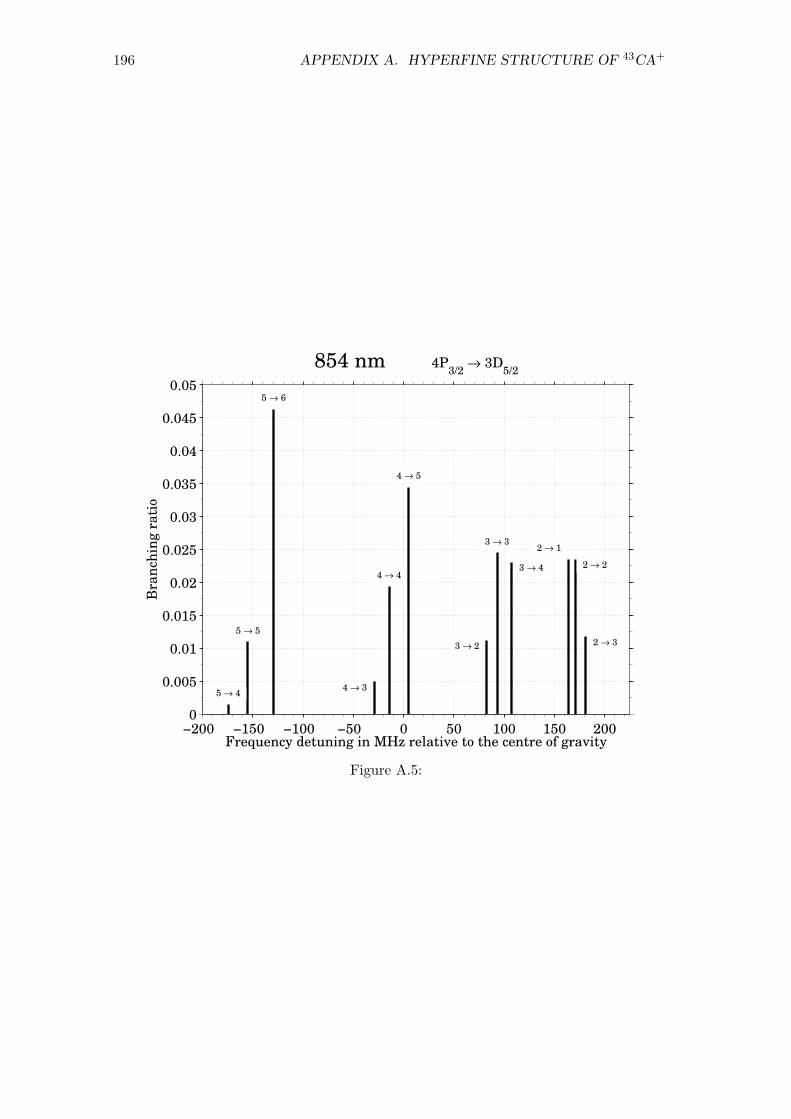
196 APPENDIX A. HYPERFINE STRUCTURE OF 43CA+
−200 −150 −100 −50 0 50 100 150 2000
0.005
0.01
0.015
0.02
0.025
0.03
0.035
0.04
0.045
0.05
Frequency detuning in MHz relative to the centre of gravity
Bra
nch
ing r
ati
o
854 nm 4P3/2
→ 3D5/2
2 → 1
2 → 2
3 → 2 2 → 3
3 → 3
4 → 3
3 → 44 → 4
5 → 4
4 → 5
5 → 5
5 → 6
Figure A.5:
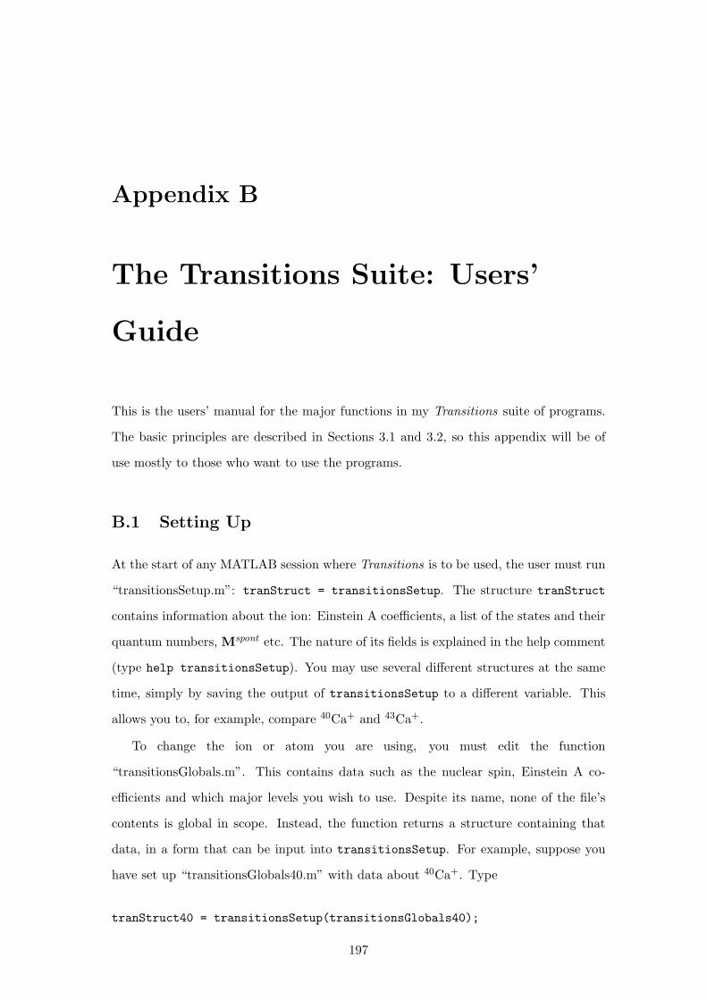
Appendix B
The Transitions Suite: Users’
Guide
This is the users’ manual for the major functions in my Transitions suite of programs.
The basic principles are described in Sections 3.1 and 3.2, so this appendix will be of
use mostly to those who want to use the programs.
B.1 Setting Up
At the start of any MATLAB session where Transitions is to be used, the user must run
“transitionsSetup.m”: tranStruct = transitionsSetup. The structure tranStruct
contains information about the ion: Einstein A coefficients, a list of the states and their
quantum numbers, Mspont etc. The nature of its fields is explained in the help comment
(type help transitionsSetup). You may use several different structures at the same
time, simply by saving the output of transitionsSetup to a different variable. This
allows you to, for example, compare 40Ca+ and 43Ca+.
To change the ion or atom you are using, you must edit the function
“transitionsGlobals.m”. This contains data such as the nuclear spin, Einstein A co-
efficients and which major levels you wish to use. Despite its name, none of the file’s
contents is global in scope. Instead, the function returns a structure containing that
data, in a form that can be input into transitionsSetup. For example, suppose you
have set up “transitionsGlobals40.m” with data about 40Ca+. Type
tranStruct40 = transitionsSetup(transitionsGlobals40);
197

198 APPENDIX B. THE TRANSITIONS SUITE: USERS’ GUIDE
to use it. If transitionsSetup is given no input, it uses “transitionsGlobals.m” by
default. Currently, “transitionsGlobals.m” is set up for 43Ca+.
The command tranStruct.levData = transitionsZeemanData
(tranStruct, B) will apply a magnetic field B to the ion. B is in Tesla: 1 T = 104 G.
You may use this command as often as you wish to change the field. Only the linear
Zeeman shifts are calculated, and no attempt is made to mix the states.
B.2 Adding and Using Lasers
Initially, no laser light exists in the model. Lasers are stored in matrices, with each row
representing a laser. Suppose you already have a list of lasers, called lasers (if you
don’t, simply define it as the empty matrix [] or ), that you wish to add to. Use the
command:
lasers = transitionsAddLaser(tranStruct, lasers, ...
newName oldName intensity detuning);
where newName is a string that you wish to call the new laser; intensity is the intial
intensity of the laser in saturation intensities; detuning is the frequency difference, in
s−1 (angular units), between the laser and the centre-of-gravity of the sublevels of the
level addressed by the laser. oldName is a string specifying a template on which to
base your laser. An oldName of ’866+’ causes your new laser to be 866 nm with a
polarisation of σ+. ’397|’ or ’850-’ define 397 nm π polarised or 850 nm σ− polarised
lasers respectively. 854 nm and 393 nm are available as well. A laser of a particular
wavelength is assumed to address one fine-structure line only, e.g. using ’866+’ means
that your laser will only affect the 4P1/2 ↔ 3D3/2 transition (but all the hyperfine
components of it) no matter what its detuning. To define new template lasers (e.g. for
using a different type of ion), edit “transitionsGlobals.m”.
The newName given to a laser when it was created allows you to change its detuning
or intensity at any time. Use
lasers = transitionsChangeDetuning(lasers, name, detuning);
to change the detuning of the laser called name, stored in the matrix lasers, to detuning
s−1 (use detuning*2e6*pi to specify detuning in MHz).
lasers = transitionsChangeIntensity(lasers, name, intensity);

B.3. SOLVING 199
works similarly for intensity in I0.
Although Mspont is generated by transitionsSetup and stored in tranStruct, you
must keep track of Mstim yourself. The matrix of stimulated transitions due to the set
of lasers lasers is calculated by
stimMatrix = transitionsGenStim(tranStruct, lasers);
It is a good idea to keep at least two different laser lists and Mstims: one for lasers that
you keep fixed, and one for lasers being scanned. This will make your simulation faster.
B.3 Solving
This code finds the steady state sublevel populations:
transMatrix = spontMatrix + stimMatrix1 + stimMatrix2 + ...;
solution = transitionsSteadySolve(transMatrix);
The vector solution contains the population of each sublevel. You do not need to worry
about adding the normalisation constraint manually: transitionsSteadySolve does it
for you.
There is no special function for handling time-dependent modelling, but we only
need MATLAB’s own matrix exponential function expm. Given a time in seconds, and
an initial vector of populations initial the code
pulseMatrix = expm(transMatrix*time);
final = pulseMatrix * initial;
returns final, the population vector that results from evolving initial for time sec-
onds.
Sometimes we want to keep transMatrix constant and calculate how the populations
change over time. In this case we can gain a significant speed-up by splitting the matrix
exponential into two parts (algorithm by Simon Webster). First run
[v,d]=eig(transMatrix);
once to calculate the eigenvectors v and eigenvalues d. Then, inside the loop that scans
the time, we can use
pulseMatrix = real(v*diag(exp(diag(d*time)))/v);
The speed gain is a factor of ∼ 2.
200 APPENDIX B. THE TRANSITIONS SUITE: USERS’ GUIDE
B.4 Utility Functions
The indices corresponding to each level are listed in Table B.1.
Level Starts at Row Ends at Row
4S1/2 1 16
3D3/2 17 48
3D5/2 49 96
4P1/2 97 112
4P3/2 113 144
Table B.1: Indices of the 43Ca+ levels in the matrices and vectors produced by the
Transitions functions
The routine transitionsLevFind can be used to find the indices of a particular set
of states. For instance,
transitionsLevFind(tranStruct, 4, [1,0], 1/2, 3, 0)
tells you that the 4S3,01/2 and 4P3,0
1/2 substates can be found at indices 4 and 100 (NOT
necessarily respectively). The order of arguments (after the data structure) is n, L, J ,
F , MF . Any of the arguments can be scalar, vector or matrix. One or more of the
rightmost arguments may be omitted to allow that quantum number to take any value.
E.g.
transitionsLevFind(tranStruct, [3,4], [0,1,2], 3/2)
finds the indices of all states with n = 3 or 4, L = 0, 1 or 2 and J = 3/2. It can also
understand spectroscopic notation:
transitionsLevFind(tranStruct, ’4P_1/2(4,4)’)
The underscore “_” or the braces “” can be omitted. But if hyperfine components are
specified they must be in parentheses “()”. The function transitionsSpecNote (by
Andrew Steane) converts between spectroscopic notation and [n, L, J , F , MF ] lists, in
either direction.
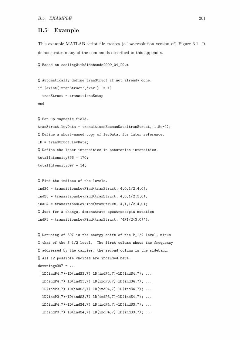
B.5. EXAMPLE 201
B.5 Example
This example MATLAB script file creates (a low-resolution version of) Figure 3.1. It
demonstrates many of the commands described in this appendix.
% Based on coolingWithSidebands2009_04_29.m
% Automatically define tranStruct if not already done.
if (exist(’tranStruct’,’var’) ~= 1)
tranStruct = transitionsSetup
end
% Set up magnetic field.
tranStruct.levData = transitionsZeemanData(tranStruct, 1.5e-4);
% Define a short-named copy of levData, for later reference.
lD = tranStruct.levData;
% Define the laser intensities in saturation intensities.
totalIntensity866 = 170;
totalIntensity397 = 14;
% Find the indices of the levels.
indS4 = transitionsLevFind(tranStruct, 4,0,1/2,4,0);
indS3 = transitionsLevFind(tranStruct, 4,0,1/2,3,0);
indP4 = transitionsLevFind(tranStruct, 4,1,1/2,4,0);
% Just for a change, demonstrate spectroscopic notation.
indP3 = transitionsLevFind(tranStruct, ’4P1/2(3,0)’);
% Detuning of 397 is the energy shift of the P_1/2 level, minus
% that of the S_1/2 level. The first column shows the frequency
% addressed by the carrier; the second column is the sideband.
% All 12 possible choices are included here.
detunings397 = ...
[lD(indP4,7)-lD(indS3,7) lD(indP4,7)-lD(indS4,7); ...
lD(indP4,7)-lD(indS3,7) lD(indP3,7)-lD(indS4,7); ...
lD(indP3,7)-lD(indS3,7) lD(indP4,7)-lD(indS4,7); ...
lD(indP3,7)-lD(indS3,7) lD(indP3,7)-lD(indS4,7); ...
lD(indP4,7)-lD(indS4,7) lD(indP4,7)-lD(indS3,7); ...
lD(indP3,7)-lD(indS4,7) lD(indP4,7)-lD(indS3,7); ...
202 APPENDIX B. THE TRANSITIONS SUITE: USERS’ GUIDE
lD(indP4,7)-lD(indS4,7) lD(indP3,7)-lD(indS3,7); ...
lD(indP3,7)-lD(indS4,7) lD(indP3,7)-lD(indS3,7); ...
lD(indP4,7)-lD(indS3,7) lD(indP3,7)-lD(indS3,7); ...
lD(indP3,7)-lD(indS3,7) lD(indP4,7)-lD(indS3,7); ...
lD(indP4,7)-lD(indS4,7) lD(indP3,7)-lD(indS4,7); ...
lD(indP3,7)-lD(indS4,7) lD(indP4,7)-lD(indS4,7)];
% Frequency values to plot in MHz. Change the number between the
% colons to change the resolution. I used 5 for my plot in the
% thesis.
freqs = -1500:50:2000;
% Predefine the array that will hold the results, for efficiency.
results = zeros(length(freqs),12);
% Loop over all choices of 397 carrier and sideband frequency.
for itD = 1:12
detuning397c = detunings397(itD,1);
detuning397s = detunings397(itD,2);
% Carrier: has 74% of the total 397 intensity.
lasersFixed = [];
lasersFixed = transitionsAddLaser(tranStruct, lasersFixed, ...
’397c+’,’397+’, totalIntensity397*0.74/2, detuning397c);
lasersFixed = transitionsAddLaser(tranStruct, lasersFixed, ...
’397c-’,’397-’, totalIntensity397*0.74/2, detuning397c);
% Sideband: has 13% of the total 397 intensity.
lasersFixed = transitionsAddLaser(tranStruct, lasersFixed, ...
’397s+’,’397+’, totalIntensity397*0.13/2, detuning397s);
lasersFixed = transitionsAddLaser(tranStruct, lasersFixed, ...
’397s-’,’397-’, totalIntensity397*0.13/2, detuning397s);
% Calculate the stimulated transitions matrix for the fixed 397nm
% laser.
stimMatrixFixed = transitionsGenStim(tranStruct, lasersFixed);
% The spontaneous decay matrix is also constant, so we can add
% these two fixed matrices together now to reduce the amount of
% work the program does at each data point.
transMatrixFixed = (stimMatrixFixed + tranStruct.spontMatrix);
B.5. EXAMPLE 203
lasersScanned = [];
% 866 beam. Its detuning is initially set to 0, because we’ll
% scan it soon.
lasersScanned = transitionsAddLaser(tranStruct, lasersScanned,...
’866+’,’866+’, totalIntensity866/2, 0);
lasersScanned = transitionsAddLaser(tranStruct, lasersScanned,...
’866-’,’866-’, totalIntensity866/2, 0);
for itF = 1:length(freqs)
% Change detuning.
freq = freqs(itF);
lasersScanned=transitionsChangeDetuning(lasersScanned, ...
’866+’, (freq)*2*pi*1e6);
lasersScanned=transitionsChangeDetuning(lasersScanned, ...
’866-’, (freq)*2*pi*1e6);
stimMatrixScan = transitionsGenStim(tranStruct, lasersScanned);
transMatrix = transMatrixFixed + stimMatrixScan;
% Actually find the steady-state populations here.
solutionVector = transitionsSteadySolve(transMatrix);
% Add together the populations of all of the P_1/2 states, and
% save as a result.
results(itF,itD) = sum(solutionVector(97:112));
end
end
%%
% Plot a graph of the results
figure1 = figure(’Color’,[1 1 1], ’Visible’,’on’);
figure(figure1);
axes1 = axes(’Parent’,figure1);
% Choose some pretty colours.
coloursSat = 1;

204 APPENDIX B. THE TRANSITIONS SUITE: USERS’ GUIDE
coloursVal = 0.75;
colours = [0 coloursSat coloursVal; 1/4 coloursSat coloursVal; ...
1/2 coloursSat coloursVal; 3/4 coloursSat coloursVal];
plot(axes1, freqs’,results(:,1),’-’,’Color’,hsv2rgb(colours(1,:)));
hold(’on’)
plot(axes1, freqs’,results(:,2),’-’,’Color’,hsv2rgb(colours(2,:)));
plot(axes1, freqs’,results(:,3),’-’,’Color’,hsv2rgb(colours(3,:)));
plot(axes1, freqs’,results(:,4),’-’,’Color’,hsv2rgb(colours(4,:)));
plot(axes1, freqs’,results(:,5),’:’,’Color’,hsv2rgb(colours(1,:)));
plot(axes1, freqs’,results(:,6),’:’,’Color’,hsv2rgb(colours(2,:)));
plot(axes1, freqs’,results(:,7),’:’,’Color’,hsv2rgb(colours(3,:)));
plot(axes1, freqs’,results(:,8),’:’,’Color’,hsv2rgb(colours(4,:)));
% Add a horizontal line indicating the experimental result, 4.7%
plot(axes1, [freqs(1) freqs(end)],[0.047 0.047],’--k’);
set(axes1, ’XGrid’,’on’, ’YGrid’,’on’, ...
’XMinorTick’,’on’, ’YMinorTick’,’on’)
xlabel(axes1, ’866 Frequency Relative to Centre of Gravity / MHz’);
ylabel(axes1, ’Population of P_1/2’);
% Define the legend that explains the colour code of the lines.
% Sorry it looks such a mess; each line of the legend had to be
% chopped in half to fit LaTeX’s line-length limit.
legend(...
[’Carrier on S_1/2^3\rightarrow P_1/2^4;’...
’ Sideband on S_1/2^4\rightarrow P_1/2^4’], ...
[’Carrier on S_1/2^3\rightarrow P_1/2^4;’...
’ Sideband on S_1/2^4\rightarrow P_1/2^3’], ...
[’Carrier on S_1/2^3\rightarrow P_1/2^3;’...
’ Sideband on S_1/2^4\rightarrow P_1/2^4’], ...
[’Carrier on S_1/2^3\rightarrow P_1/2^3;’...
’ Sideband on S_1/2^4\rightarrow P_1/2^3’], ...
[’Carrier on S_1/2^4\rightarrow P_1/2^4;’...
’ Sideband on S_1/2^3\rightarrow P_1/2^4’], ...
[’Carrier on S_1/2^4\rightarrow P_1/2^3;’...
’ Sideband on S_1/2^3\rightarrow P_1/2^4’], ...

B.5. EXAMPLE 205
[’Carrier on S_1/2^4\rightarrow P_1/2^4;’...
’ Sideband on S_1/2^3\rightarrow P_1/2^3’], ...
[’Carrier on S_1/2^4\rightarrow P_1/2^3;’...
’ Sideband on S_1/2^3\rightarrow P_1/2^3’], ...
’Experimental P Population: 4.7%’)

206 APPENDIX B. THE TRANSITIONS SUITE: USERS’ GUIDE
Bibliography
Numbers at the end of each bibliography item indicate the page(s) on which that refer-
ence is cited.
[1] C. Oseen, “The Nobel prize in physics 1926,” December 1926. [Online]. Available:
http://nobelprize.org/nobel prizes/physics/laureates/1926/press.html 1
[2] G. Patterson, “Jean Perrin and the triumph of the atomic doctrine,” Endeavour,
vol. 31, no. 2, pp. 50 – 53, 2007. [Online]. Available: http://www.sciencedirect.
com/science/article/B6V81-4P2S220-1/2/0c574722958fd3fec878bc3ccea0c88b 1
[3] W. Neuhauser, M. Hohenstatt, P. E. Toschek, and H. Dehmelt, “Localized visible
Ba+ mono-ion oscillator,” Physical Review A, vol. 22, no. 3, pp. 1137–1140, Sep
1980. [Online]. Available: http://link.aps.org/abstract/PRA/v22/e1137 1
[4] E. Fischer, “Die dreidimensionale Stabilisierung von Ladungstragern in einem
Vierpolfeld,” Zeitschrift Fur Physik, vol. 156, no. 1, pp. 1–26, 1959. [Online].
Available: http://www.springerlink.com/content/rv3p37027u78442k/ 1
[5] W. Paul and M. Raether, “Das elektrische massenfilter,” Zeitschrift Fur Physik,
vol. 140, no. 3, pp. 262–273, 1955. [Online]. Available: http://www.springerlink.
com/content/h0g58v83t33m5331/ 1
[6] W. Paul, “Electromagnetic traps for charged and neutral particles,” in Nobel
Lectures, Physics 1981-1990, G. Ekspang, Ed. World Scientific Publishing Co.,
Singapore, 1993. [Online]. Available: http://nobelprize.org/nobel prizes/physics/
laureates/1989/paul-lecture.pdf 1
[7] “The Nobel prize in physics 1989,” October 1989. [Online]. Available: http://
nobelprize.org/nobel prizes/physics/laureates/1989/press.html 1
207

208 BIBLIOGRAPHY
[8] S. R. Jefferts, T. P. Heavner, T. E. Parker, and J. H. Shirley, “NIST cesium
fountains - current status and future prospects,” in Time and Frequency
Metrology, ser. Proceedings of the Society of Photo-Optical Instrumentation
Engineers (SPIE), R. Jones, Ed., vol. 6673. SPIE-Int Soc Optical Engineering,
2007, Proceedings Paper, p. 67309, Conference on Time and Frequency
Metrology, San Diego, CA, AUG 29-30, 2007. [Online]. Available: http://tf.nist.
gov/timefreq/general/pdf/2254.pdf 1
[9] D. J. Wineland, W. M. Itano, J. C. Bergquist, and R. G. Hulet, “Laser-cooling
limits and single-ion spectroscopy,” Physical Review A, vol. 36, no. 5, pp.
2220–2232, Sep 1987. [Online]. Available: http://link.aps.org/abstract/PRA/
v36/e2220 2
[10] T. Rosenband, D. B. Hume, P. O. Schmidt, C. W. Chou, A. Brusch, L. Lorini,
W. H. Oskay, R. E. Drullinger, T. M. Fortier, J. E. Stalnaker, S. A. Diddams,
W. C. Swann, N. R. Newbury, W. M. Itano, D. J. Wineland, and J. C. Bergquist,
“Frequency ratio of Al+ and Hg+ single-ion optical clocks; metrology at the
17th decimal place,” Science, vol. 319, no. 5871, pp. 1808–1812, MAR 28 2008.
[Online]. Available: http://www.sciencemag.org/cgi/content/abstract/319/5871/
1808 2
[11] P. Gill, “Optical frequency standards,” Metrologia, vol. 42, no. 3, pp. S125–S137,
2005. [Online]. Available: http://stacks.iop.org/0026-1394/42/S125 2
[12] W. Neuhauser, M. Hohenstatt, P. Toschek, and H. Dehmelt, “Optical-sideband
cooling of visible atom cloud confined in parabolic well,” Physical Review Letters,
vol. 41, no. 4, pp. 233–236, Jul 1978. [Online]. Available: http://link.aps.org/
abstract/PRL/v41/e233 1, 20
[13] T. Dent, S. Stern, and C. Wetterich, “Competing bounds on the present-day
time variation of fundamental constants,” Physical Review D, vol. 79, no. 8, art.
no. 083533, 2009. [Online]. Available: http://link.aps.org/abstract/PRD/v79/
e083533 2
[14] J. Jin and D. Church, “Precision lifetimes for the Ca+ 4p 2P levels – experiment
challenges theory at the 1-percent level,” Physical Review Letters, vol. 70, no. 21,

BIBLIOGRAPHY 209
pp. 3213–3216, MAY 24 1993. [Online]. Available: http://link.aps.org/abstract/
PRL/v70/e3213 2, 16
[15] B. K. Sahoo, M. R. Islam, B. P. Das, R. K. Chaudhuri, and D. Mukherjee,
“Lifetimes of the metastable 2D3/2,5/2 states in Ca+, Sr+, and Ba+,” Physical
Review A, vol. 74, no. 6, art. no. 062504, Dec 2006. [Online]. Available: http://
link.aps.org/abstract/PRA/v74/e062504 2, 58
[16] W. Nortershauser, K. Blaum, K. Icker, P. Muller, A. Schmitt, K. Wendt, and
B. Wiche, “Isotope shifts and hyperfine structure in the 3d 2DJ → 4p 2PJ
transitions in calcium II,” European Physical Journal D, vol. 2, no. 1, pp.
33–39, May 1998. [Online]. Available: http://www.springerlink.com/content/
jw7a64lgrpuy3fme/ 2, 61, 62
[17] G. Tommaseo, T. Pfeil, G. Revalde, G. Werth, P. Indelicato, and J. Desclaux,
“The g(J)-factor in the ground state of Ca+,” European Physical Journal
D, vol. 25, no. 2, pp. 113–121, Aug 2003. [Online]. Available: http://www.
springerlink.com/content/lr6hnnr16y17vj5u/ 2, 61
[18] J. A. Sherman, T. W. Korber, A. Markhotok, W. Nagourney, and E. N. Fortson,
“Precision measurement of light shifts in a single trapped Ba+ ion,” Physical
Review Letters, vol. 94, no. 24, art. no. 243001, Jun 2005. [Online]. Available:
http://link.aps.org/abstract/PRL/v94/e243001 2
[19] J. A. Sherman, A. Andalkar, W. Nagourney, and E. N. Fortson, “Measurement
of light shifts at two off-resonant wavelengths in a single trapped Ba+ ion and
the determination of atomic dipole matrix elements,” Physical Review A, vol. 78,
no. 5, art. no. 052514, 2008. [Online]. Available: http://link.aps.org/abstract/
PRA/v78/e052514 2
[20] R. Gerritsma, G. Kirchmair, F. Zaehringer, J. Benhelm, R. Blatt, and C. F.
Roos, “Precision measurement of the branching fractions of the 4p 2P3/2 decay
of Ca II,” European Physical Journal D, vol. 50, no. 1, pp. 13–19, Nov 2008.
[Online]. Available: http://www.springerlink.com/content/fm87711l4x780363/ 2,
16, 62, 84
210 BIBLIOGRAPHY
[21] A. L. Wolf, S. A. van den Berg, C. Gohle, E. J. Salumbides, W. Ubachs, and
K. S. E. Eikema, “Frequency metrology on the 4s 2S1/2–4p 2P1/2 transition in
40Ca+ for a comparison with quasar data,” Physical Review A, vol. 78, no. 3, art.
no. 032511, Sep 2008. [Online]. Available: http://link.aps.org/abstract/PRA/
v78/e032511 2, 62
[22] N. Fortson, “Possibility of measuring parity nonconservation with a single
trapped atomic ion,” Physical Review Letters, vol. 70, no. 16, pp. 2383–2386, Apr
1993. [Online]. Available: http://link.aps.org/abstract/PRL/v70/e2383 2
[23] L. W. Wansbeek, B. K. Sahoo, R. G. E. Timmermans, K. Jungmann, B. P. Das,
and D. Mukherjee, “Atomic parity nonconservation in Ra+,” Physical Review A,
vol. 78, no. 5, art. no. 050501, 2008. [Online]. Available: http://link.aps.org/
abstract/PRA/v78/e050501 2
[24] D. Weiss, B. Young, and S. Chu, “Precision measurement of h/mCs based
on photon recoil using laser-cooled atoms and atomic interferometry,” Applied
Physics B, vol. 59, no. 3, pp. 217–256, Sep 1994. [Online]. Available: http://
www.springerlink.com/content/w2703mp20t144426/ 3
[25] I. Bergstrom, C. Carlberg, T. Fritioff, G. Douysset, J. Schonfelder, and
R. Schuch, “SMILETRAP – a Penning trap facility for precision mass
measurements using highly charged ions,” Nuclear Instruments and Methods in
Physics Research Section A, vol. 487, no. 3, pp. 618 – 651, 2002. [Online].
Available: http://www.sciencedirect.com/science/article/B6TJM-44T51MJ-8/2/
968a349c77ff47f271667a43156b9734 3
[26] G. Gabrielse, “Antiproton mass measurements,” International Journal of
Mass Spectrometry, vol. 251, no. 2-3, pp. 273 – 280, 2006. [Online].
Available: http://www.sciencedirect.com/science/article/B6VND-4JN2KP5-1/
2/a9f2c409cbd28763bc4764c3253c93e2 3
[27] R. S. Van Dyck, P. B. Schwinberg, and H. G. Dehmelt, “New high-precision
comparison of electron and positron g factors,” Physical Review Letters, vol. 59,
no. 1, pp. 26–29, Jul 1987. [Online]. Available: http://link.aps.org/abstract/
PRL/v59/e26 3

BIBLIOGRAPHY 211
[28] D. Hanneke, S. Fogwell, and G. Gabrielse, “New measurement of the electron
magnetic moment and the fine structure constant,” Physical Review Letters,
vol. 100, no. 12, art. no. 120801, 2008. [Online]. Available: http://link.aps.org/
abstract/PRL/v100/e120801 3
[29] R. P. Feynman, “Simulating physics with computers,” International Journal of
Theoretical Physics, vol. 21, no. 6-7, pp. 467–488, 1982. [Online]. Available:
http://www.springerlink.com/content/t2x8115127841630/ 3
[30] S. Lloyd, “Universal quantum simulators,” Science, vol. 273, no. 5278, pp.
1073–1078, 1996. [Online]. Available: http://www.sciencemag.org/cgi/content/
abstract/273/5278/1073 3
[31] S. Lloyd, “Universal quantum simulators: Correction,” Science, vol. 279, no.
5354, pp. 1113h–1117, 1998. [Online]. Available: http://www.sciencemag.org/
cgi/content/short/279/5354/1113h 3
[32] D. Deutsch, “Quantum theory, the Church-Turing principle and the universal
quantum computer,” Proceedings of the Royal Society of London. Series A,
Mathematical and Physical Sciences, vol. 400, no. 1818, pp. 97–117, 1985.
[Online]. Available: http://www.jstor.org/stable/2397601 4
[33] D. Deutsch and R. Jozsa, “Rapid solution of problems by quantum computation,”
Proceedings: Mathematical and Physical Sciences, vol. 439, no. 1907, pp. 553–558,
1992. [Online]. Available: http://www.jstor.org/stable/52182 4
[34] R. Cleve, A. Ekert, C. Macchiavello, and M. Mosca, “Quantum algorithms
revisited,” Proceedings: Mathematical, Physical and Engineering Sciences, vol.
454, no. 1969, pp. 339–354, 1998. [Online]. Available: http://www.jstor.org/
stable/53169 4
[35] P. W. Shor, “Polynomial-time algorithms for prime factorization and discrete
logarithms on a quantum computer,” SIAM Journal on Computing, vol. 26,
no. 5, pp. 1484–1509, 1997. [Online]. Available: http://link.aip.org/link/?SMJ/
26/1484/1 4

212 BIBLIOGRAPHY
[36] L. K. Grover, “Quantum mechanics helps in searching for a needle in a haystack,”
Physical Review Letters, vol. 79, no. 2, pp. 325–328, Jul 1997. [Online]. Available:
http://link.aps.org/abstract/PRL/v79/e325 4
[37] E. Novak, “Quantum complexity of integration,” Journal of Complexity, vol. 17,
no. 1, pp. 2 – 16, 2001. [Online]. Available: http://www.sciencedirect.com/
science/article/B6WHX-45BC224-11/2/d150612b685c45d796026a0ab5211f18 4
[38] S. P. Jordan, “Quantum algorithm zoo,” May 2009, adapted from the first
chapter of the author’s PhD thesis (Quantum Computation Beyond the Circuit
Model, http://arxiv.org/abs/0809.2307). [Online]. Available: http://www.its.
caltech.edu/∼sjordan/zoo.html 4
[39] D. DiVincenzo, “The physical implementation of quantum computation,”
Fortschritte der Physik, vol. 48, no. 9-11, pp. 771–783, 2000. [Online]. Available:
http://www3.interscience.wiley.com/journal/74000505/abstract 4
[40] T. C. Ralph, K. J. Resch, and A. Gilchrist, “Efficient toffoli gates using qudits,”
Physical Review A (Atomic, Molecular, and Optical Physics), vol. 75, no. 2, art.
no. 022313, 2007. [Online]. Available: http://link.aps.org/abstract/PRA/v75/
e022313 4
[41] B. P. Lanyon, M. Barbieri, M. P. Almeida, T. Jennewein, T. C. Ralph, K. J.
Resch, G. J. Pryde, J. L. O’Brien, A. Gilchrist, and A. G. White, “Simplifying
quantum logic using higher-dimensional hilbert spaces,” Nature Physics, vol. 5,
no. 2, pp. 134–140, Feb 2009. [Online]. Available: http://www.nature.com/
nphys/journal/v5/n2/abs/nphys1150.html 4
[42] M. A. Nielsen and I. L. Chuang, Quantum Computation and Quantum Informa-
tion. 5
[43] W. Wootters and W. Zurek, “A single quantum cannot be cloned,” Nature, vol.
299, no. 5886, pp. 802–803, 1982. [Online]. Available: http://www.nature.com/
nature/journal/v299/n5886/abs/299802a0.html 5
[44] D. Dieks, “Communication by epr devices,” Physics Letters A, vol. 92, no. 6,
pp. 271 – 272, 1982. [Online]. Available: http://www.sciencedirect.com/science/
article/B6TVM-46R3NRJ-12W/2/361098ee0d55c300114ee9ad7cff6aab 5
BIBLIOGRAPHY 213
[45] L. Vandersypen, M. Steffen, G. Breyta, C. Yannoni, M. Sherwood, and
I. Chuang, “Experimental realization of Shor’s quantum factoring algorithm using
nuclear magnetic resonance,” Nature, vol. 414, no. 6866, pp. 883–887, DEC 20
2001. [Online]. Available: http://www.nature.com/nature/journal/v414/n6866/
abs/414883a.html 6
[46] “A quantum information science and technology roadmap,” April 2004. [Online].
Available: http://qist.lanl.gov/qcomp map.shtml 6
[47] P. Walther, K. Resch, T. Rudolph, E. Schenck, H. Weinfurter, V. Vedral,
M. Aspelmeyer, and A. Zeilinger, “Experimental one-way quantum computing,”
Nature, vol. 434, no. 7030, pp. 169–176, MAR 10 2005. [Online]. Available:
http://www.nature.com/nature/journal/v434/n7030/abs/nature03347.html 6
[48] R. Prevedel, P. Walther, F. Tiefenbacher, P. Bohl, R. Kaltenbaek, T. Jennewein,
and A. Zeilinger, “High-speed linear optics quantum computing using active feed-
forward,” Nature, vol. 445, no. 7123, pp. 65–69, JAN 4 2007. [Online]. Available:
http://www.nature.com/nature/journal/v445/n7123/abs/nature05346.html 6
[49] J. L. O’Brien, “Optical quantum computing,” Science, vol. 318, no. 5856, pp.
1567–1570, 2007. [Online]. Available: http://www.sciencemag.org/cgi/content/
abstract/318/5856/1567 6
[50] H. J. Briegel, D. E. Browne, W. Duer, R. Raussendorf, and M. Van den Nest,
“Measurement-based quantum computation,” Nature Physics, vol. 5, no. 1, pp.
19–26, JAN 2009. [Online]. Available: http://www.nature.com/nphys/journal/
v5/n1/abs/nphys1157.html 6
[51] L. DiCarlo, J. M. Chow, J. M. Gambetta, L. S. Bishop, B. R. Johnson,
D. I. Schuster, J. Majer, A. Blais, L. Frunzio, S. M. Girvin, and R. J.
Schoelkopf, “Demonstration of two-qubit algorithms with a superconducting
quantum processor,” Nature, vol. 460, no. 7252, pp. 240–244, JUL 9 2009.
[Online]. Available: http://www.nature.com/nature/journal/v460/n7252/abs/
nature08121.html 6

214 BIBLIOGRAPHY
[52] S. Das Sarma, M. Freedman, and C. Nayak, “Topological quantum computation,”
Physics Today, vol. 59, no. 7, pp. 32–38, Jul 2006. [Online]. Available: http://dx.
doi.org/10.1063/1.2337825 6
[53] D. Aharonov, W. van Dam, J. Kempe, Z. Landau, S. Lloyd, and
O. Regev, “Adiabatic quantum computation is equivalent to standard quantum
computation,” SIAM Review, vol. 50, no. 4, pp. 755–787, Dec 2008. [Online].
Available: http://dx.doi.org/10.1137/080734479 6
[54] H. Haffner, C. F. Roos, and R. Blatt, “Quantum computing with trapped
ions,” Physics Reports, vol. 469, no. 4, pp. 155–203, Dec 2008. [Online].
Available: http://www.sciencedirect.com/science/article/B6TVP-4TJTX51-1/2/
20e335f01bd298a35ec14f54a234ea19 7
[55] P. Barton, C. Donald, D. Lucas, D. Stevens, A. Steane, and D. Stacey,
“Measurement of the lifetime of the 3d 2D5/2 state in 40Ca+,” Physical Review
A, vol. 62, no. 3, art. no. 032503, Sep 2000. [Online]. Available: http://link.aps.
org/abstract/PRA/v62/e032503 7, 16, 31, 62, 75, 76
[56] C. F. Roos, M. Chwalla, K. Kim, M. Riebe, and R. Blatt, “ ‘Designer atoms’
for quantum metrology,” Nature, vol. 443, no. 7109, pp. 316–319, SEP 21
2006. [Online]. Available: http://www.nature.com/nature/journal/v443/n7109/
abs/nature05101.html 7
[57] S. Olmschenk, K. C. Younge, D. L. Moehring, D. N. Matsukevich, P. Maunz,
and C. Monroe, “Manipulation and detection of a trapped Yb+ hyperfine qubit,”
Physical Review A, vol. 76, no. 5, art. no. 052314, Nov 2007. [Online]. Available:
http://link.aps.org/abstract/PRA/v76/e052314 7, 82, 130, 131
[58] D. M. Lucas, B. C. Keitch, J. P. Home, G. Imreh, M. J. McDonnell, D. N.
Stacey, D. J. Szwer, and A. M. Steane, “A long-lived memory qubit on a
low-decoherence quantum bus,” arXiv, art. no. 0710.4421v1, Oct. 2007. [Online].
Available: http://arxiv.org/abs/0710.4421 8, 13, 17, 77, 161, 174
[59] C. Langer, R. Ozeri, J. Jost, J. Chiaverini, B. DeMarco, A. Ben-Kish,
R. Blakestad, J. Britton, D. Hume, W. Itano, D. Leibfried, R. Reichle,
T. Rosenband, T. Schaetz, P. Schmidt, and D. Wineland, “Long-lived qubit
BIBLIOGRAPHY 215
memory using atomic ions,” Physical Review Letters, vol. 95, no. 6, art. no.
060502, AUG 5 2005. [Online]. Available: http://link.aps.org/abstract/PRL/
v95/e060502 8
[60] J. Bollinger, D. Heinzen, W. Itano, S. Gilbert, and D. Wineland, “A
303-MHz frequency standard based on trapped Be+ ions,” IEEE Transactions on
Instrumentation and Measurement, vol. 40, no. 2, pp. 126–128, Apr 1991. [Online].
Available: http://ieeexplore.ieee.org/search/wrapper.jsp?arnumber=1032897 8
[61] J. Chiaverini, D. Leibfried, T. Schaetz, M. Barrett, R. Blakestad, J. Britton,
W. Itano, J. Jost, E. Knill, C. Langer, R. Ozeri, and D. Wineland, “Realization
of quantum error correction,” Nature, vol. 432, no. 7017, pp. 602–605, DEC 2
2004. [Online]. Available: http://www.nature.com/nature/journal/v432/n7017/
abs/nature03074.html 8, 11, 13
[62] J. Chiaverini, J. Britton, D. Leibfried, E. Knill, M. Barrett, R. Blakestad,
W. Itano, J. Jost, C. Langer, R. Ozeri, T. Schaetz, and D. Wineland,
“Implementation of the semiclassical quantum fourier transform in a scalable
system,” Science, vol. 308, no. 5724, pp. 997–1000, MAY 13 2005. [Online].
Available: http://www.sciencemag.org/cgi/content/abstract/308/5724/997 8, 11,
13, 161
[63] M. Johanning, A. Braun, N. Timoney, V. Elman, W. Neuhauser, and
C. Wunderlich, “Individual addressing of trapped ions and coupling of motional
and spin states using rf radiation,” Physical Review Letters, vol. 102, no. 7, art.
no. 073004, 2009. [Online]. Available: http://link.aps.org/abstract/PRL/v102/
e073004 8
[64] S. X. Wang, J. Labaziewicz, Y. Ge, R. Shewmon, and I. L. Chuang, “Individual
addressing of ions using magnetic field gradients in a surface-electrode ion trap,”
Applied Physics Letters, vol. 94, no. 9, p. 094103, 2009. [Online]. Available:
http://link.aip.org/link/?APL/94/094103/1 8
[65] P. Haljan, P. Lee, K. Brickman, M. Acton, L. Deslauriers, and C. Monroe,
“Entanglement of trapped-ion clock states,” Physical Review A, vol. 72, no. 6,
art. no. 062316, Dec 2005. [Online]. Available: http://link.aps.org/abstract/
PRA/v72/e062316 8, 9

216 BIBLIOGRAPHY
[66] D. Leibfried, “Individual addressing and state readout of trapped ions utilizing rf
micromotion,” Physical Review A, vol. 60, no. 5, pp. R3335–R3338, Nov 1999.
[Online]. Available: http://prola.aps.org/abstract/PRA/v60/i5/pR3335 1 8, 18
[67] J. Cirac and P. Zoller, “Quantum computations with cold trapped ions,” Physical
Review Letters, vol. 74, no. 20, pp. 4091–4094, MAY 15 1995. [Online]. Available:
http://link.aps.org/abstract/PRL/v74/e4091 8
[68] C. Monroe, D. M. Meekhof, B. E. King, W. M. Itano, and D. J. Wineland,
“Demonstration of a fundamental quantum logic gate,” Phys. Rev. Lett., vol. 75,
no. 25, pp. 4714–4717, Dec 1995. [Online]. Available: http://link.aps.org/
abstract/PRL/v75/e4714 8
[69] M. Riebe, K. Kim, P. Schindler, T. Monz, P. O. Schmidt, T. K. Korber,
W. Hansel, H. Haffner, C. F. Roos, and R. Blatt, “Process tomography of ion
trap quantum gates,” Physical Review Letters, vol. 97, no. 22, art. no. 220407,
DEC 1 2006. [Online]. Available: http://link.aps.org/abstract/PRL/v97/e220407
9
[70] A. Sørensen and K. Mølmer, “Entanglement and quantum computation with ions
in thermal motion,” Physical Review A, vol. 62, no. 2, art. no. 022311, Aug 2000.
[Online]. Available: http://link.aps.org/abstract/PRA/v62/e022311 9, 134
[71] J. Benhelm, G. Kirchmair, C. F. Roos, and R. Blatt, “Towards fault-tolerant
quantum computing with trapped ions,” Nature Physics, vol. 4, no. 6, pp.
463–466, Jun 2008. [Online]. Available: http://www.nature.com/nphys/journal/
v4/n6/abs/nphys961.html 9, 82
[72] G. Kirchmair, J. Benhelm, F. Zahringer, R. Gerritsma, C. F. Roos, and R. Blatt,
“High-fidelity entanglement of 43Ca+ hyperfine clock states,” Physical Review A,
vol. 79, no. 2, art. no. 020304, 2009. [Online]. Available: http://link.aps.org/
abstract/PRA/v79/e020304 9, 82, 131
[73] D. Leibfried, B. DeMarco, V. Meyer, D. Lucas, M. Barrett, J. Britton, W. Itano,
B. Jelenkovic, C. Langer, T. Rosenband, and D. Wineland, “Experimental
demonstration of a robust, high-fidelity geometric two ion-qubit phase gate,”
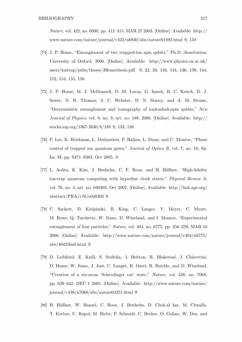
BIBLIOGRAPHY 217
Nature, vol. 422, no. 6930, pp. 412–415, MAR 27 2003. [Online]. Available: http://
www.nature.com/nature/journal/v422/n6930/abs/nature01492.html 9, 134
[74] J. P. Home, “Entanglement of two trapped-ion spin qubits,” Ph.D. dissertation,
University of Oxford, 2006. [Online]. Available: http://www.physics.ox.ac.uk/
users/iontrap/pubs/theses/JHomethesis.pdf 9, 22, 33, 133, 134, 136, 139, 144,
152, 154, 155, 156
[75] J. P. Home, M. J. McDonnell, D. M. Lucas, G. Imreh, B. C. Keitch, D. J.
Szwer, N. R. Thomas, S. C. Webster, D. N. Stacey, and A. M. Steane,
“Deterministic entanglement and tomography of ion–spin qubits,” New
Journal of Physics, vol. 8, no. 9, art. no. 188, 2006. [Online]. Available: http://
stacks.iop.org/1367-2630/8/188 9, 133, 138
[76] P. Lee, K. Brickman, L. Deslauriers, P. Haljan, L. Duan, and C. Monroe, “Phase
control of trapped ion quantum gates,” Journal of Optics B, vol. 7, no. 10, Sp.
Iss. SI, pp. S371–S383, Oct 2005. 9
[77] L. Aolita, K. Kim, J. Benhelm, C. F. Roos, and H. Haffner, “High-fidelity
ion-trap quantum computing with hyperfine clock states,” Physical Review A,
vol. 76, no. 4, art. no. 040303, Oct 2007. [Online]. Available: http://link.aps.org/
abstract/PRA/v76/e040303 9
[78] C. Sackett, D. Kielpinski, B. King, C. Langer, V. Meyer, C. Myatt,
M. Rowe, Q. Turchette, W. Itano, D. Wineland, and I. Monroe, “Experimental
entanglement of four particles,” Nature, vol. 404, no. 6775, pp. 256–259, MAR 16
2000. [Online]. Available: http://www.nature.com/nature/journal/v404/n6775/
abs/404256a0.html 9
[79] D. Leibfried, E. Knill, S. Seidelin, J. Britton, R. Blakestad, J. Chiaverini,
D. Hume, W. Itano, J. Jost, C. Langer, R. Ozeri, R. Reichle, and D. Wineland,
“Creation of a six-atom ‘Schrodinger cat’ state,” Nature, vol. 438, no. 7068,
pp. 639–642, DEC 1 2005. [Online]. Available: http://www.nature.com/nature/
journal/v438/n7068/abs/nature04251.html 9
[80] H. Haffner, W. Hansel, C. Roos, J. Benhelm, D. Chek-al kar, M. Chwalla,
T. Korber, U. Rapol, M. Riebe, P. Schmidt, C. Becher, O. Guhne, W. Dur, and

218 BIBLIOGRAPHY
R. Blatt, “Scalable multiparticle entanglement of trapped ions,” Nature, vol. 438,
no. 7068, pp. 643–646, DEC 1 2005. [Online]. Available: http://www.nature.
com/nature/journal/v438/n7068/abs/nature04279.html 9
[81] F. Mintert and C. Wunderlich, “Ion-trap quantum logic using long-wavelength
radiation,” Physical Review Letters, vol. 87, no. 25, art. no. 257904, DEC 17
2001. [Online]. Available: http://link.aps.org/abstract/PRL/v87/e257904 10
[82] A. H. Myerson, D. J. Szwer, S. C. Webster, D. T. C. Allcock, M. J. Curtis,
G. Imreh, J. A. Sherman, D. N. Stacey, A. M. Steane, and D. M. Lucas,
“High-fidelity readout of trapped-ion qubits,” Physical Review Letters, vol. 100,
no. 20, art. no. 200502, MAY 23 2008. [Online]. Available: http://link.aps.org/
abstract/PRL/v100/e200502 10, 36, 73, 82, 128, 130
[83] H. Dehmelt, “Proposed 1014δν > ν laser fluorescence spectroscopy on Tl+ mono-
ion oscillator ii,” Bulletin of the American Physical Society, vol. 20, no. 1, p. 60,
1975. 10
[84] A. H. Burrell, D. J. Szwer, S. C. Webster, and D. M. Lucas, “Scalable simultaneous
multi-qubit readout with 99.99% single-shot fidelity,” 2009, In preparation. 10
[85] D. B. Hume, T. Rosenband, and D. J. Wineland, “High-fidelity adaptive qubit
detection through repetitive quantum nondemolition measurements,” Physical
Review Letters, vol. 99, no. 12, art. no. 120502, SEP 21 2007. [Online]. Available:
http://link.aps.org/abstract/PRL/v99/e120502 11, 130
[86] R. Stock and D. F. V. James, “Scalable, high-speed measurement-based quantum
computer using trapped ions,” Physical Review Letters, vol. 102, no. 17, art.
no. 170501, 2009. [Online]. Available: http://link.aps.org/abstract/PRL/v102/
e170501 11, 81
[87] M. Riebe, M. Chwalla, J. Benhelm, H. Haffner, W. Hansel, C. F. Roos, and
R. Blatt, “Quantum teleportation with atoms: quantum process tomography,”
New Journal of Physics, vol. 9, no. 7, art. no. 211, 2007. [Online]. Available:
http://stacks.iop.org/1367-2630/9/211 11
[88] M. Barrett, J. Chiaverini, T. Schaetz, J. Britton, W. Itano, J. Jost, E. Knill,
C. Langer, D. Leibfried, R. Ozeri, and D. Wineland, “Deterministic quantum
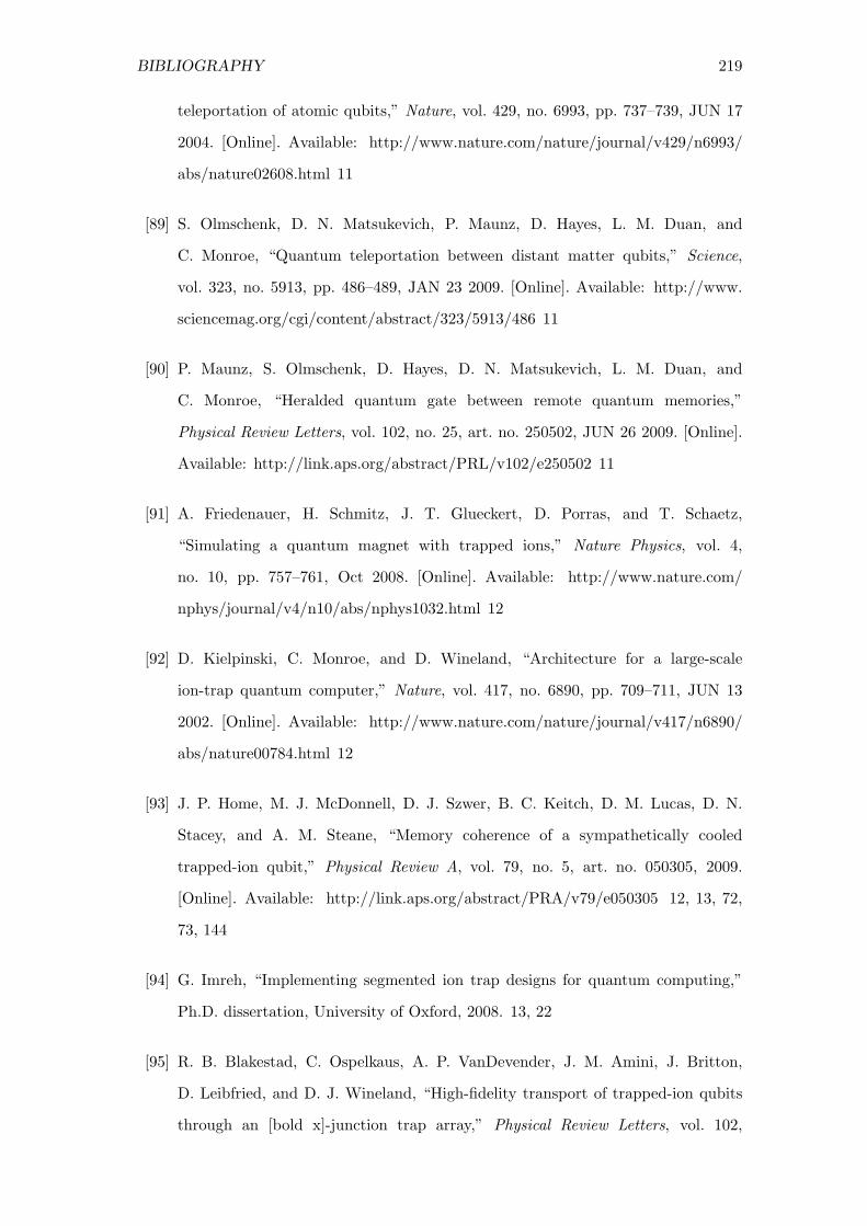
BIBLIOGRAPHY 219
teleportation of atomic qubits,” Nature, vol. 429, no. 6993, pp. 737–739, JUN 17
2004. [Online]. Available: http://www.nature.com/nature/journal/v429/n6993/
abs/nature02608.html 11
[89] S. Olmschenk, D. N. Matsukevich, P. Maunz, D. Hayes, L. M. Duan, and
C. Monroe, “Quantum teleportation between distant matter qubits,” Science,
vol. 323, no. 5913, pp. 486–489, JAN 23 2009. [Online]. Available: http://www.
sciencemag.org/cgi/content/abstract/323/5913/486 11
[90] P. Maunz, S. Olmschenk, D. Hayes, D. N. Matsukevich, L. M. Duan, and
C. Monroe, “Heralded quantum gate between remote quantum memories,”
Physical Review Letters, vol. 102, no. 25, art. no. 250502, JUN 26 2009. [Online].
Available: http://link.aps.org/abstract/PRL/v102/e250502 11
[91] A. Friedenauer, H. Schmitz, J. T. Glueckert, D. Porras, and T. Schaetz,
“Simulating a quantum magnet with trapped ions,” Nature Physics, vol. 4,
no. 10, pp. 757–761, Oct 2008. [Online]. Available: http://www.nature.com/
nphys/journal/v4/n10/abs/nphys1032.html 12
[92] D. Kielpinski, C. Monroe, and D. Wineland, “Architecture for a large-scale
ion-trap quantum computer,” Nature, vol. 417, no. 6890, pp. 709–711, JUN 13
2002. [Online]. Available: http://www.nature.com/nature/journal/v417/n6890/
abs/nature00784.html 12
[93] J. P. Home, M. J. McDonnell, D. J. Szwer, B. C. Keitch, D. M. Lucas, D. N.
Stacey, and A. M. Steane, “Memory coherence of a sympathetically cooled
trapped-ion qubit,” Physical Review A, vol. 79, no. 5, art. no. 050305, 2009.
[Online]. Available: http://link.aps.org/abstract/PRA/v79/e050305 12, 13, 72,
73, 144
[94] G. Imreh, “Implementing segmented ion trap designs for quantum computing,”
Ph.D. dissertation, University of Oxford, 2008. 13, 22
[95] R. B. Blakestad, C. Ospelkaus, A. P. VanDevender, J. M. Amini, J. Britton,
D. Leibfried, and D. J. Wineland, “High-fidelity transport of trapped-ion qubits
through an [bold x]-junction trap array,” Physical Review Letters, vol. 102,
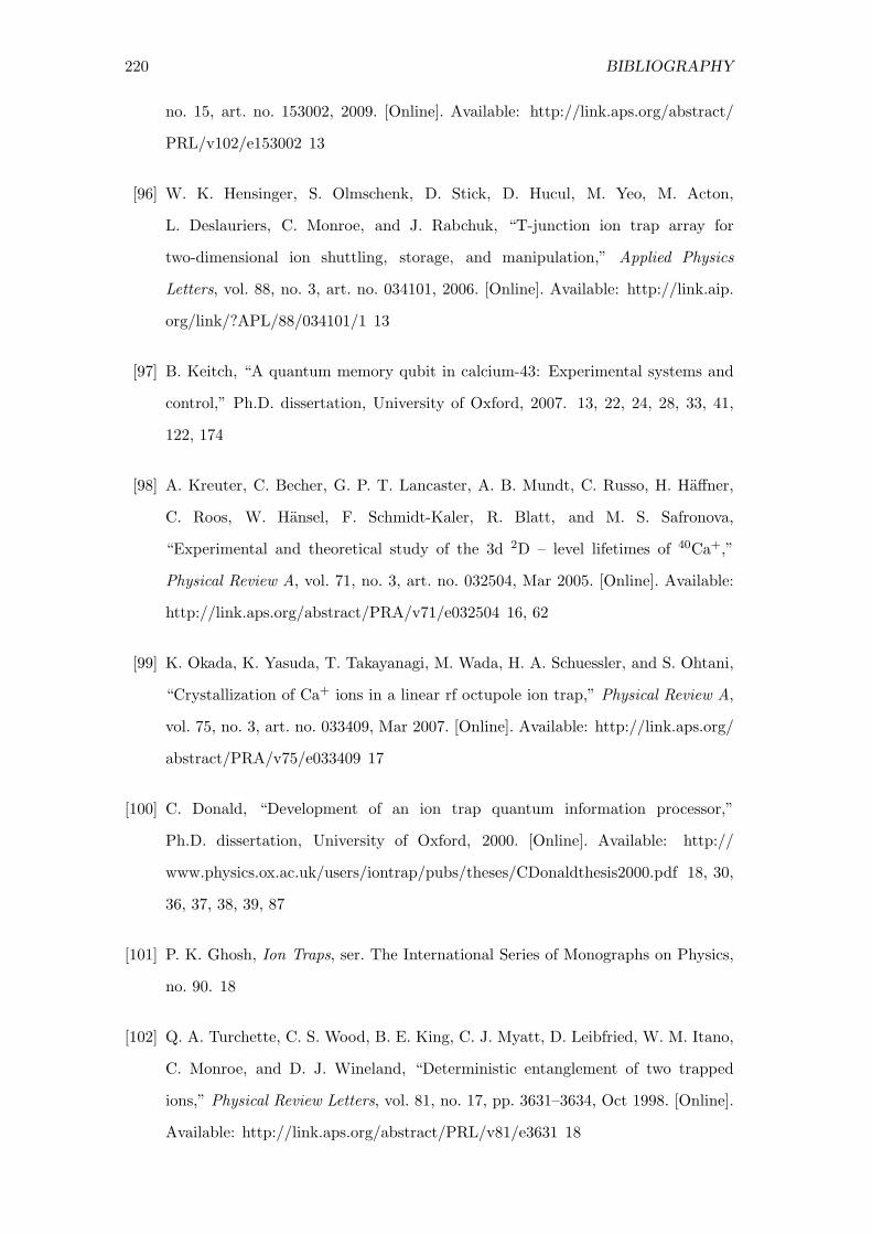
220 BIBLIOGRAPHY
no. 15, art. no. 153002, 2009. [Online]. Available: http://link.aps.org/abstract/
PRL/v102/e153002 13
[96] W. K. Hensinger, S. Olmschenk, D. Stick, D. Hucul, M. Yeo, M. Acton,
L. Deslauriers, C. Monroe, and J. Rabchuk, “T-junction ion trap array for
two-dimensional ion shuttling, storage, and manipulation,” Applied Physics
Letters, vol. 88, no. 3, art. no. 034101, 2006. [Online]. Available: http://link.aip.
org/link/?APL/88/034101/1 13
[97] B. Keitch, “A quantum memory qubit in calcium-43: Experimental systems and
control,” Ph.D. dissertation, University of Oxford, 2007. 13, 22, 24, 28, 33, 41,
122, 174
[98] A. Kreuter, C. Becher, G. P. T. Lancaster, A. B. Mundt, C. Russo, H. Haffner,
C. Roos, W. Hansel, F. Schmidt-Kaler, R. Blatt, and M. S. Safronova,
“Experimental and theoretical study of the 3d 2D – level lifetimes of 40Ca+,”
Physical Review A, vol. 71, no. 3, art. no. 032504, Mar 2005. [Online]. Available:
http://link.aps.org/abstract/PRA/v71/e032504 16, 62
[99] K. Okada, K. Yasuda, T. Takayanagi, M. Wada, H. A. Schuessler, and S. Ohtani,
“Crystallization of Ca+ ions in a linear rf octupole ion trap,” Physical Review A,
vol. 75, no. 3, art. no. 033409, Mar 2007. [Online]. Available: http://link.aps.org/
abstract/PRA/v75/e033409 17
[100] C. Donald, “Development of an ion trap quantum information processor,”
Ph.D. dissertation, University of Oxford, 2000. [Online]. Available: http://
www.physics.ox.ac.uk/users/iontrap/pubs/theses/CDonaldthesis2000.pdf 18, 30,
36, 37, 38, 39, 87
[101] P. K. Ghosh, Ion Traps, ser. The International Series of Monographs on Physics,
no. 90. 18
[102] Q. A. Turchette, C. S. Wood, B. E. King, C. J. Myatt, D. Leibfried, W. M. Itano,
C. Monroe, and D. J. Wineland, “Deterministic entanglement of two trapped
ions,” Physical Review Letters, vol. 81, no. 17, pp. 3631–3634, Oct 1998. [Online].
Available: http://link.aps.org/abstract/PRL/v81/e3631 18

BIBLIOGRAPHY 221
[103] J. M. Amini, J. Britton, D. Leibfried, and D. J. Wineland, Atom Chips, ch.
Microfabricated Chip Traps for Ions. [Online]. Available: http://arxiv.org/abs/
0812.3907 19
[104] Q. Turchette, D. Kielpinski, B. King, D. Leibfried, D. Meekhof, C. Myatt,
M. Rowe, C. Sackett, C. Wood, W. Itano, C. Monroe, and D. Wineland,
“Heating of trapped ions from the quantum ground state,” Physical Review A,
vol. 61, no. 6, art. no. 063418, Jun 2000. [Online]. Available: http://prola.aps.
org/abstract/PRA/v61/i6/e063418 19
[105] L. Deslauriers, S. Olmschenk, D. Stick, W. K. Hensinger, J. Sterk, and
C. Monroe, “Scaling and suppression of anomalous heating in ion traps,” Physical
Review Letters, vol. 97, no. 10, art. no. 103007, SEP 8 2006. [Online]. Available:
http://link.aps.org/abstract/PRL/v97/e103007 19
[106] D. M. Lucas, A. Ramos, J. P. Home, M. J. McDonnell, S. Nakayama, J.-P. Stacey,
S. C. Webster, D. N. Stacey, and A. M. Steane, “Isotope-selective photoionization
for calcium ion trapping,” Physical Review A, vol. 69, art. no. 012711, 2004.
[Online]. Available: http://link.aps.org/abstract/PRA/v69/e012711 21, 22, 62
[107] D. Allcock, “A multi-channel laser diagnostic system for trapped-ion quantum
computing experiments,” University of Oxford, Tech. Rep., 2007. 27
[108] M. McDonnell, “Two-photon readout methods for an ion trap quantum
information processor,” Ph.D. dissertation, University of Oxford, 2003.
[Online]. Available: http://www.physics.ox.ac.uk/users/iontrap/pubs/theses/
McDonnellthesis2003.pdf 28, 69, 82
[109] J.-P. Stacey, “Stabilization and control in a linear ion trap,” Ph.D. dissertation,
University of Oxford, 2003. [Online]. Available: http://www.physics.ox.ac.uk/
users/iontrap/pubs/theses/JPStaceythesis.pdf 30
[110] S. Webster, “Raman sideband cooling and coherent manipulation or trapped
ions,” DPhil thesis, University of Oxford, 2005. [Online]. Available: http://
www.physics.ox.ac.uk/users/iontrap/pubs/theses/SWebsterthesis2005.pdf 32, 51,
54, 55, 86

222 BIBLIOGRAPHY
[111] K. P. Zetie, “Parity non-conservation in atomic bismuth,” Ph.D. dissertation,
University of Oxford, 1991. 44
[112] ThorLabs Catalogue, 18th ed., ThorLabs, Inc, 2006. 44
[113] G. Imreh, “Polarization maintaining fiber,” University of Oxford, Tech. Rep., Jan-
uary 2007. 47
[114] R. D. Cowan, The Theory of Atomic Structure and Spectra, ser. Los Alamos Series
in Basic and Applied Sciences. 54, 55, 56, 57
[115] B. W. Shore and D. H. Menzel, Principles of Atomic Spectra. 57
[116] M. Melendez, M. A. Bautista, and N. R. Badnell, “Atomic data
from the IRON project - LXIV. radiative transition rates and collision
strengths for CaII,” Astronomy & Astrophysics, vol. 469, no. 3, pp.
1203–1209, Jul 2007. [Online]. Available: http://www.aanda.org/index.php?
option=article&access=doi&doi=10.1051/0004-6361:20077262 58
[117] N. A. Jelley, Fundamentals of Nuclear Physics. 59
[118] M. V. Romalis, W. C. Griffith, J. P. Jacobs, and E. N. Fortson, “New limit
on the permanent electric dipole moment of 199Hg,” Physical Review Letters,
vol. 86, no. 12, pp. 2505–2508, Mar 2001. [Online]. Available: http://link.aps.
org/abstract/PRL/v86/e2505 59
[119] G. K. Woodgate, Elementary Atomic Structure, 2nd ed. 59
[120] F. Arbes, M. Benzing, T. Gudjons, F. Kurth, and G. Werth, “Precise
determination of the ground-state hyperfine-structure splitting of Ca-43-II,”
Zeitschrift Fur Physik D, vol. 31, no. 1-2, pp. 27–30, Aug 1994. [Online].
Available: http://www.springerlink.com/content/r87801u3467l61k7/ 61
[121] J. Benhelm, G. Kirchmair, U. Rapol, T. Korber, C. F. Roos, and R. Blatt,
“Measurement of the hyperfine structure of the S1/2–D5/2 transition in 43Ca+,”
Physical Review A, vol. 75, no. 3, art. no. 032506, Mar 2007. [Online]. Available:
http://link.aps.org/abstract/PRA/v75/e032506 61, 62
[122] J. Benhelm, G. Kirchmair, U. Rapol, T. Korber, C. F. Roos, and R. Blatt,
“Erratum: Measurement of the hyperfine structure of the S1/2–D5/2 transition in

BIBLIOGRAPHY 223
43Ca+ (vol 75, pg 032506, 2007),” Physical Review A, vol. 75, no. 4, art. no.
049901, Apr 2007. [Online]. Available: http://link.aps.org/abstract/PRA/v75/
e049901 61
[123] M. Chwalla, J. Benhelm, K. Kim, G. Kirchmair, T. Monz, M. Riebe, P. Schindler,
A. Villar, C. F. Roos, W. Hansel, and R. Blatt, “Absolute frequency measurement
of 40Ca+ in a paul trap,” in 2008 Conference On Precision Electromagnetic Mea-
surements Digest, A. Cookson and T. Winter, Eds., 2008, pp. 94–95, conference
on Precision Electromagnetic Measurements, Broomfield, CO, JUN 08-13, 2008.
61, 62
[124] A. L. Wolf, S. A. van den Berg, W. Ubachs, and K. S. E. Eikema, “Direct
frequency comb spectroscopy of trapped ions,” Physical Review Letters, vol. 102,
no. 22, art. no. 223901, JUN 5 2009. [Online]. Available: http://link.aps.org/
abstract/PRL/v102/e223901 62
[125] Y. Ralchenko, A. . Kramida, J. Reader, and NIST ASD Team, “NIST atomic
spectra database (version 3.1.5),” 2008. [Online]. Available: http://physics.nist.
gov/asd3 62
[126] B. Edlen and P. Risberg, “The spectrum of singly-ionized calcium, Ca-II,” Arkiv
For Fysik, vol. 10, no. 6, pp. 553–566, 1956. 62
[127] D. J. Berkeland and M. G. Boshier, “Destabilization of dark states and optical
spectroscopy in Zeeman-degenerate atomic systems,” Physical Review A, vol. 65,
art. no. 033413, 2002. [Online]. Available: http://link.aps.org/abstract/PRA/
v65/e033413 66, 68
[128] J. Benhelm, G. Kirchmair, C. F. Roos, and R. Blatt, “Experimental quantum-
information processing with 43Ca+ ions,” Physical Review A, vol. 77, no. 6, art.
no. 062306, Jun 2008. [Online]. Available: http://link.aps.org/abstract/PRA/
v77/e062306 68, 82, 107, 131
[129] J. Benhelm, “Precision spectroscopy and quantum information processing
with trapped calcium ions,” Ph.D. dissertation, University of Innsbruck, May
2008. [Online]. Available: http://heart-c704.uibk.ac.at/publications/dissertation/
benhelm diss.pdf 68

224 BIBLIOGRAPHY
[130] D. Stacey, “Summary of progress on solving the Bloch equations for 43Ca,” Uni-
versity of Oxford, Tech. Rep., 2007. 69
[131] D. Stacey, “Fitting Ca43 scans from 14th November 2008,” University of Oxford,
Tech. Rep., 2009. 71
[132] M. Kajita, Y. Li, K. Matsubara, K. Hayasaka, and M. Hosokawa, “Prospect of
optical frequency standard based on a 43Ca+ ion,” Physical Review A, vol. 72,
no. 4, art. no. 043404, Oct 2005. [Online]. Available: http://link.aps.org/
abstract/PRA/v72/e043404 71, 79
[133] D. T. C. Allcock, J. A. Sherman, M. J. Curtis, G. Imreh, A. H. Burrell
(nee Myerson), D. J. Szwer, D. N. Stacey, A. M. Steane, and D. M.
Lucas, “Implementation of a symmetric surface electrode ion trap with field
compensation using a modulated Raman effect,” arXiv, art. no. 0909.3272, 2009.
[Online]. Available: http://arxiv.org/abs/0909.3272 72
[134] A. M. Steane, “How to build a 300 bit, 1 giga-operation quantum computer,”
Quantum Information & Computation, vol. 7, no. 3, pp. 171–183, Mar
2007. [Online]. Available: http://www.physics.ox.ac.uk/users/iontrap/pubs/
Steane 2004.pdf 81, 112, 126
[135] R. Raussendorf, J. Harrington, and K. Goyal, “A fault-tolerant one-way quantum
computer,” Annals of Physics, vol. 321, no. 9, pp. 2242 – 2270, 2006. [Online].
Available: http://www.sciencedirect.com/science/article/B6WB1-4JRVD64-1/2/
7874b1702eb19a942b8b71dbbcf299b7 81
[136] M. Acton, K. A. Brickman, P. C. Haljan, P. J. Lee, L. Deslauriers, and
C. Monroe, “Near-perfect simultaneous measurement of a qubit register,”
Quantum Information & Computation, vol. 6, no. 6, pp. 465–482, Sep 2006.
[Online]. Available: http://arxiv.org/abs/quant-ph/0511257 82, 130, 131
[137] S. Huard, Polarization of Light. 86
[138] Optimization Toolbox 4 Users Guide, Version 4.2 (release 2009a) ed., The
MathWorks, Inc, March 2009. [Online]. Available: http://www.mathworks.com/
access/helpdesk/help/pdf doc/optim/optim tb.pdf 87

BIBLIOGRAPHY 225
[139] J. D’Errico, “Optimization tips and tricks,” December 2006. [Online]. Available:
http://www.mathworks.com/matlabcentral/fileexchange/8553 88
[140] E. Hecht and A. Zajac, Optics, 1st ed. 126
[141] M. J. Biercuk, H. Uys, A. P. VanDevender, N. Shiga, W. M. Itano, and J. J.
Bollinger, “Optimized dynamical decoupling in a model quantum memory,”
Nature, vol. 458, no. 7241, pp. 996–1000, APR 23 2009. [Online]. Available:
http://www.nature.com/nature/journal/v458/n7241/abs/nature07951.html 129,
161, 172, 173, 185
[142] (2009) ThorLabs online catalogue. Electronic. [Online]. Available: http://www.
thorlabs.com/navigation.cfm?Guide ID=24 129
[143] N. Kurz, M. R. Dietrich, G. Shu, R. Bowler, J. Salacka, V. Mirgon, and B. B.
Blinov, “Measurement of the branching ratio in the 6P3/2 decay of Ba II with
a single trapped ion,” Physical Review A, vol. 77, no. 6, art. no. 060501, 2008.
[Online]. Available: http://link.aps.org/abstract/PRA/v77/e060501 130, 131
[144] C. Wunderlich, T. Hannemann, T. Korber, H. Haffner, C. Roos, W. Hansel,
R. Blatt, and F. Schmidt-Kaler, “Robust state preparation of a single trapped ion
by adiabatic passage,” Journal of Modern Optics, vol. 54, no. 11, pp. 1541–1549,
2007. [Online]. Available: http://www.informaworld.com/smpp/content∼db=all?
content=10.1080/09500340600741082 131
[145] M. R. Dietrich, A. Avril, R. Bowler, N. Kurz, J. S. Salacka, G. Shu, and B. B.
Blinov, “Barium ions for quantum computation,” arXiv, art. no. 0905.2701v1,
May 2009. [Online]. Available: http://arxiv.org/abs/0905.2701 131
[146] W. Nagourney, J. Sandberg, and H. Dehmelt, “Shelved optical electron amplifier:
Observation of quantum jumps,” Physical Review Letters, vol. 56, no. 26, pp.
2797–2799, Jun 1986. [Online]. Available: http://prola.aps.org/abstract/PRL/
v56/i26/p2797 1 131
[147] A. A. Madej and J. D. Sankey, “Quantum jumps and the single trapped barium
ion: Determination of collisional quenching rates for the 5d 2D5/2 level,” Physical
Review A, vol. 41, no. 5, pp. 2621–2630, Mar 1990. [Online]. Available: http://
prola.aps.org/abstract/PRA/v41/i5/p2621 1 131
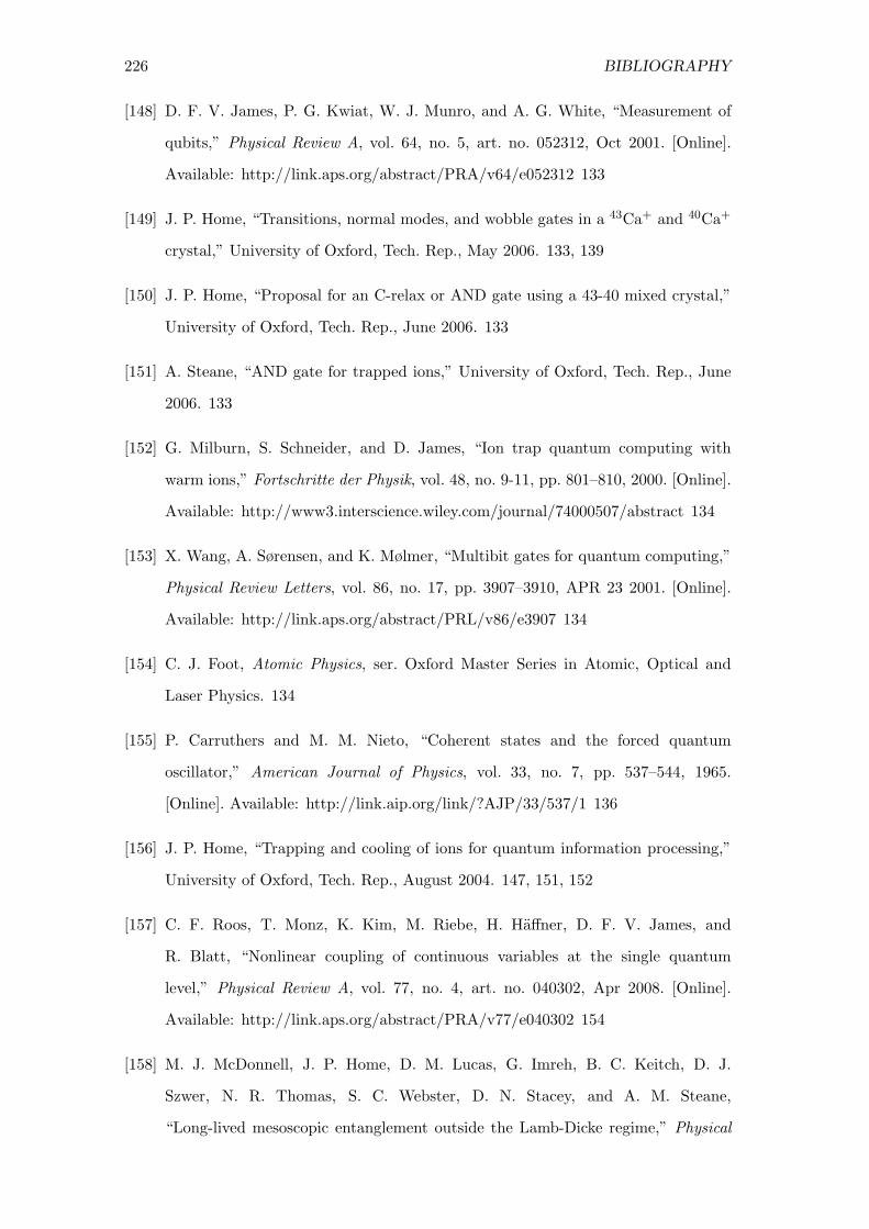
226 BIBLIOGRAPHY
[148] D. F. V. James, P. G. Kwiat, W. J. Munro, and A. G. White, “Measurement of
qubits,” Physical Review A, vol. 64, no. 5, art. no. 052312, Oct 2001. [Online].
Available: http://link.aps.org/abstract/PRA/v64/e052312 133
[149] J. P. Home, “Transitions, normal modes, and wobble gates in a 43Ca+ and 40Ca+
crystal,” University of Oxford, Tech. Rep., May 2006. 133, 139
[150] J. P. Home, “Proposal for an C-relax or AND gate using a 43-40 mixed crystal,”
University of Oxford, Tech. Rep., June 2006. 133
[151] A. Steane, “AND gate for trapped ions,” University of Oxford, Tech. Rep., June
2006. 133
[152] G. Milburn, S. Schneider, and D. James, “Ion trap quantum computing with
warm ions,” Fortschritte der Physik, vol. 48, no. 9-11, pp. 801–810, 2000. [Online].
Available: http://www3.interscience.wiley.com/journal/74000507/abstract 134
[153] X. Wang, A. Sørensen, and K. Mølmer, “Multibit gates for quantum computing,”
Physical Review Letters, vol. 86, no. 17, pp. 3907–3910, APR 23 2001. [Online].
Available: http://link.aps.org/abstract/PRL/v86/e3907 134
[154] C. J. Foot, Atomic Physics, ser. Oxford Master Series in Atomic, Optical and
Laser Physics. 134
[155] P. Carruthers and M. M. Nieto, “Coherent states and the forced quantum
oscillator,” American Journal of Physics, vol. 33, no. 7, pp. 537–544, 1965.
[Online]. Available: http://link.aip.org/link/?AJP/33/537/1 136
[156] J. P. Home, “Trapping and cooling of ions for quantum information processing,”
University of Oxford, Tech. Rep., August 2004. 147, 151, 152
[157] C. F. Roos, T. Monz, K. Kim, M. Riebe, H. Haffner, D. F. V. James, and
R. Blatt, “Nonlinear coupling of continuous variables at the single quantum
level,” Physical Review A, vol. 77, no. 4, art. no. 040302, Apr 2008. [Online].
Available: http://link.aps.org/abstract/PRA/v77/e040302 154
[158] M. J. McDonnell, J. P. Home, D. M. Lucas, G. Imreh, B. C. Keitch, D. J.
Szwer, N. R. Thomas, S. C. Webster, D. N. Stacey, and A. M. Steane,
“Long-lived mesoscopic entanglement outside the Lamb-Dicke regime,” Physical

BIBLIOGRAPHY 227
Review Letters, vol. 98, no. 6, art. no. 063603, FEB 9 2007. [Online]. Available:
http://link.aps.org/abstract/PRL/v98/e063603 156
[159] E. L. Hahn, “Spin echoes,” Physical Review, vol. 80, no. 4, pp. 580–594, Nov
1950. [Online]. Available: http://prola.aps.org/abstract/PR/v80/i4/p580 1 161
[160] L. Viola and S. Lloyd, “Dynamical suppression of decoherence in two-state
quantum systems,” Physical Review A, vol. 58, no. 4, pp. 2733–2744, Oct 1998.
[Online]. Available: http://prola.aps.org/abstract/PRA/v58/i4/p2733 1 161
[161] N. F. Ramsey, “A new molecular beam resonance method,” Physical Review,
vol. 76, no. 7, p. 996, Oct 1949. [Online]. Available: http://prola.aps.org/
abstract/PR/v76/i7/p996 1 162
[162] G. S. Uhrig, “Exact results on dynamical decoupling by π pulses in quantum
information processes,” New Journal of Physics, vol. 10, no. 8, art. no. 083024,
2008. [Online]. Available: http://stacks.iop.org/1367-2630/10/083024 165, 168,
171
[163] Sin[z]ˆ(2 n). Wolfram Research, Inc. [Online]. Available: http://functions.
wolfram.com/01.06.16.0103.01 167
[164] Sum[(–1)ˆk cos[a k], k, 0, n]. Wolfram Research, Inc. [Online]. Available:
http://functions.wolfram.com/01.07.23.0002.01 167
[165] Sum[(–1)ˆk sin[a k], k, 0, n]. Wolfram Research, Inc. [Online]. Available:
http://functions.wolfram.com/01.06.23.0002.01 167
[166] G. S. Uhrig, “Keeping a quantum bit alive by optimized π-pulse sequences,”
Physical Review Letters, vol. 98, no. 10, art. no. 100504, MAR 9 2007. [Online].
Available: http://link.aps.org/abstract/PRL/v98/e100504 171
[167] B. Lee, W. M. Witzel, and S. Das Sarma, “Universal pulse sequence to minimize
spin depahasing in the central spin decoherence problem,” Physical Review
Letters, vol. 100, no. 16, art. no. 160505, APR 25 2008. [Online]. Available:
http://link.aps.org/abstract/PRL/v100/e160505 171
[168] D. Dhar, L. Grover, and S. Roy, “Preserving quantum states using inverting
pulses: a super-Zeno effect,” Physical Review Letters, vol. 96, no. 10, art. no.

228 BIBLIOGRAPHY
100405, MAR 17 2006. [Online]. Available: http://link.aps.org/abstract/PRL/
v96/e100405 172
[169] L. Cywinski, R. M. Lutchyn, C. P. Nave, and S. Das Sarma, “How to enhance
dephasing time in superconducting qubits,” Physical Review B, vol. 77, no. 17,
art. no. 174509, May 2008. [Online]. Available: http://link.aps.org/abstract/
PRB/v77/e174509 172, 183, 184
[170] M. J. Biercuk, H. Uys, A. P. VanDevender, N. Shiga, W. M. Itano, and
J. J. Bollinger, “Experimental Uhrig dynamical decoupling using trapped ions,”
Physical Review A, vol. 79, no. 6, art. no. 062324, 2009. [Online]. Available:
http://link.aps.org/abstract/PRA/v79/e062324 172, 185
[171] R. Freeman, Spin Choreography: Basic Steps in High Resolution NMR. 172
[172] H. Uys, M. J. Biercuk, and J. J. Bollinger, “Optimized noise filtration through
dynamical decoupling,” Physical Review Letters, vol. 103, no. 4, art. no. 040501,
2009. [Online]. Available: http://link.aps.org/abstract/PRL/v103/e040501 172,
173


![See beyond the Bridge…. and further still...600mmF2.4-4 large-aperture high-magnification zoom lens • High-fidelity capture of image detail and fast readout with 20.1MP[ii] 1.0-type](https://cdn.vdocuments.site/doc/165x107/60e5d5038ef8343b0a1d10a8/see-beyond-the-bridge-and-further-still-600mmf24-4-large-aperture-high-magnification.jpg)


