JPL Publication 88-35
High-Dynamic GPS Tracking Final Report
S. Hinedi J. 1. Statman
December 15,1988
Prepared for
U.S. Air Force Systems Command Armament Division
National Aeronautics and Space Administration by
Jet Propulsion Laboratory
Through an agreement with
California Institute of Technology Pasadena, California
https://ntrs.nasa.gov/search.jsp?R=19890010742 2019-03-26T08:02:17+00:00Z
The research described in this publication was carried out by the Jet Propulsion Laboratory, California Institute of Technology, and was sponsored by the United States Air Force Systems Command, Armament Division through an agreement with the National Aeronautics and Space Administration.
Reference herein to any specific commercial product, process, or service by trade name, trademark, manufacturer, or otherwise, does not constitute or imply its endorsement by the United States Government or the Jet Propulsion Laboratory, California Institute of Technology.
ABSTRACT
This report presents the results of comparing four different frequency estimation schemes in the presence of high dynamics at low carrier-to-noise ratios.
The comparison is based on measured data from a hardware demonstration. The tested algorithms include a digital phase-locked loop, a cross-product automatic frequency tracking loop, an extended Kalman filter, and finally, an FFT-aided cross-product frequency tracking loop. The tracking algorithms are compared on their frequency error performance and their ability to maintain lock during severe maneuvers at various carrier-to-noise ratios.
The measured results are shown to agree with simulation results carried out and reported previously.
iii
ACKNOWLEDGMENT
We wish to express our deepest thanks to the many people who contributed to the work presented in this report. At JPL these include Dr. William Hurd, who led the work in the early stages, Dr. Sergio Aguirre, who developed the ODAFC algorithm, simulated the FFT-CPAFC loop, assisted on analysis of other schemes and helped set up the experiment in the early stages, Dr. Unjeng Cheng, who analyzed fast acquisition techniques and the DPLL, Dr. Rajandra Kumar who developed ALS techniques, Dr. Victor Vilnrotter who analyzed the MLE, tested the FFT-CPAFC loop, and provided the calibration analysis, Ms. Beatrice Siev who coded the real-time experiment software and documented it in Appendix C, Mr. Jay Rabkin, Mr. David Brown, Mr. Gary Stevens, and Dr. Craig Cheetam who kept the experiment functioning, and Ms. Gail Huddleston who documented it all. At Interstate Electronics Corporation (IEC) we wish to thank Mr. Larry Wells and Mr. Ken Blankshain for their assistance with the FFT-aided algorithm and for several figures. Last, but not least, we thank RAJPO, especially Mr. Thomas Hancock, Cap. Steve Shaffer, and Dr. Sultan Mahmood for their on-going support.
iv
Table of Contents Abstract ................................................................................. iii
Acknowledgment ......................................................................... iv
Table of Contents ......................................................................... v
List of Figures ........................................................................... vii
List of Tables ............................................................................ ix
1 Summary ................................................................................. 1 1.1 Executive Summary .................................................................. 1 1.2 Objectives and Approach ............................................................. 2 1.3 Results ............................................................................... 3 1.4 Conclusions and Recommendations .................................................... 3
2 Purpose and Scope ........................................................................ 5 2.1 Purpose .............................................................................. 5 2.2 Scope ................................................................................. 5
3 Introduction .............................................................................. 6 3.1 History ............................................................................... 6 3.2 Outline of Completed Research ....................................................... 6 3.3 Definition Of High-Dynamic Trajectory ............................................... 7
4 Algorithm Descriptions ................................................................... 12 4.1 Maximum Likelihood Estimator (MLE) .............................................. 12 4.2 Extended Kalman Filter (EKF) ...................................................... 13 4.3 Cross-Product AFC (CPAFC) Loop .................................................. 13 4.4 Digital Phase-Locked Loop (DPLL) .................................................. 14 4.5 Overlapping DFT AFC (ODAFC) Loop .............................................. 14 4.6 Frequency Extended Kalman Filter (FEKF) .......................................... 14
4.8 Adaptive Least Squares (ALS) ....................................................... 17 Fast Frequency Acquisition .................................................... 17
4.8.2 Differential Sampling for Fast Acquisition ...................................... 17
4.7 FFT-CPAFC LOOP .................................................................. 15
4.8.1
4.9 Signal Acquisition Algorithms ....................................................... 17 18 4.10 Performance Comparison via Simulations ...........................................
5 Description of Experimental Setup ....................................................... 22 5.1 Advanced Receiver Block Diagram ................................................... 22 5.2 Modifications to the ARX ........................................................... 24
5.2.1 Hardware Modifications ....................................................... 24 5.2.2 Software Modifications ........................................................ 24
V
6 Algorithm Evaluation .................................................................... 28 6.1 Static Test Results .................................................................. 30
6.1.1 DPLL ......................................................................... 30 6.1.2 CPAFC ....................................................................... 32
6.1.4 FFT-CPAFC .................................................................. 35 6.2 Dynamic Test Results ............................................................... 39
6.2.1 DPLL ......................................................................... 39 6.2.2 CPAFC ....................................................................... 39
6.2.4 FFT-CPAFC .................................................................. 47 6.3 Comparison and Discussion .......................................................... 47
7 Conclusions .............................................................................. 58
6.1.3 EKF .......................................................................... 32
6.2.3 EKF .......................................................................... 39
Appendices
A Description and Analysis of the FFT-CPAFC Loop ....................................... 59 A.l Simulation Results .................................................................. 59 A.2 Nonlinear Analysis .................................................................. 64
A.2.1 Static Case ................................................................... 64 A.2.2 Dynamic Case ................................................................ 68
B Calibration Measurements ............................................................... 71 B.l Mathematical Model ................................................................ 71 B.2 Estimator Structure ................................................................. 73 B.3 Numerical Results ................................................................... 75
C ARX Software Modifications ............................................................. 78
D Glossary ................................................................................. 81
E References ............................................................................... 83
vi
List of Figures
1.1 RMS frequency errors for a 100-g/s trajectory . . . . . . . . . . . . . . . . . . 4 3.2.1 8 3.3.1 Simulated 70-g/s trajectory . . . . . . . . . . . . . . . . . . . . . . . . . . . . 10 3.3.2 Simulated 100-g/s trajectory . . . . . . . . . . . . . . . . . . . . . . . . . . . . 11 4.7.1 FFT-CPAFC block diagram (figure courtesy IEC) . . . . . . . . . . . . . . . . 16 4.9.1 Fast acquisition diagram . . . . . . . . . . . . . . . . . . . . . . . . . . . . . . . 19 4.9.2 Acquisition time versus Doppler uncertainty . . . . . . . . . . . . . . . . . . . 20 5.1.1 ARX signal processing diagram . . . . . . . . . . . . . . . . . . . . . . . . . . 23 5.2.1.1 ARX hardware block diagram . . . . . . . . . . . . . . . . . . . . . . . . . . . 26 5.2.1.2 Trajectory generation hardware . . . . . . . . . . . . . . . . . . . . . . . . . . 27 6.1 Demonstration data flow . . . . . . . . . . . . . . . . . . . . . . . . . . . . . . 29 6.2 Equivalent loop gain model . . . . . . . . . . . . . . . . . . . . . . . . . . . . 30 6.1.1.1 DPLL static test results . . . . . . . . . . . . . . . . . . . . . . . . . . . . . . 31
6.1.2.2 Bias at 53 MHz . . . . . . . . . . . . . . . . . . . . . . . . . . . . . . . . . . . 34 6.1.3.1 Implementation loss in the EKF . . . . . . . . . . . . . . . . . . . . . . . . . . 36 6.1.3.2 EKF static test results . . . . . . . . . . . . . . . . . . . . . . . . . . . . . . . 37 6.1.4.1 FFT-CPAFC loop static test results . . . . . . . . . . . . . . . . . . . . . . . 38 6.2.1.1 DPLL transient response (CNR = 73 dB-Hz) . . . . . . . . . . . . . . . . . . 40 6.2.1.2 DPLL transient response (CNR = 60 dB-Hz) . . . . . . . . . . . . . . . . . . 41 6.2.1.3 DPLL dynamic test results (RMS frequency errors versus CNR) . . . . . . . . 42
43 44
. . . . 45 6.2.2.3 CPAFC loop dynamic test results (probability of loss-of-lock versus CNR) . . 46 6.2.3.1 EKF transient response (CNR = 60 dB-Hz): (a) simulation results with 100-
g/s jerk; and (b) ARX response to 100-g/s jerk . . . . . . . . . . . . . . . . . 48 49
. . . . . . 50 51
6.2.4.2 FFT-CPAFC dynamic test results (probability of loss-of-lock versus CNR) . . 52
. . . . . . 54 6.3.1 CPAFC - impact of amplitude attenuation on (a) RMS frequency error; and
(b) loss-of-lock probability . . . . . . . . . . . . . . . . . . . . . . . . . . . . . 56 A.l.1.a Transient response to 100-g/s trajectory (CNR = 30 dB-Hz) . . . . . . . . . . 60
Tracking scenario using GPS frequency translators (figure courtesy IEC) . . .
6.1.2.1 CPAFC loop static test results . . . . . . . . . . . . . . . . . . . . . . . . . . 33
6.2.1.4 DPLL dynamic test results (probability of loss-of-lock versus CNR) . . . . . . 6.2.2.1 CPAFC loop transient response (CNR = 60 dB-Hz) . . . . . . . . . . . . . . . 6.2.2.2 CPAFC loop dynamic test results (RMS frequency error versus CNR)
6.2.3.2 EKF dynamic test results (RMS frequency error versus CNR) . . . . . . . . . 6.2.3.3 EKF dynamic test results (probability of loss-of-lock versus CNR) 6.2.4.1 FFT-CPAFC dynamic test results (RMS frequency error versus CNR)
6.2.4.3 FFT-CPAFC transient response (CNR = 30 dB-Hz) . . . . . . . . . . . . . . 53 6.2.4.4 FFT-CPAFC loop response to jerk of 70 g/s, 100 g/s, and 150 g/s
. . . .
vii
A.l.l.bTransient response to 100-g/s trajectory (CNR = 25 dB-Hz) . . . . . . . . . . 61 A.l.1.c Transient response to 100-g/s trajectory (CNR = 22 dB-Hz) . . . . . . . . . . 62 A.l.1.d Transient response to 100-g/s trajectory (CNR = 50 dB-Hz) . . . . . . . . . . 63 A.1.2 RMS frequency error versus CNR for a 100-g/s trajectory . . . . . . . . . . . 65 A.1.3 Probability of loss-of-lock for a 100-g/s trajectory . . . . . . . . . . . . . . . . 66 A.2.1.1 Noise spectral density . . . . . . . . . . . . . . . . . . . . . . . . . . . . . . . 69 A.2.1.2 RMS frequency error versus CNR . . . . . . . . . . . . . . . . . . . . . . . . . 70 B.l.l Phase-locked loop block diagram . . . . . . . . . . . . . . . . . . . . . . . . . 72 B.2.1 Error envelopes as functions of CNR . . . . . . . . . . . . . . . . . . . . . . . 76 B.3.1 Calibration curve . . . . . . . . . . . . . . . . . . . . . . . . . . . . . . . . . . 77
viii
List of Tables
4.1 Performance Comparison via Simulations . . . . . . . . . . . . . . . . . . . . 21 6.1 Dynamic Test Results - RMS Frequency Error (Hz) . . . . . . . . . . . . . . 57 6.2 Dynamic Test Results - Threshold CNR . . . . . . . . . . . . . . . . . . . . . 57
ix
Chapter 1
S u m m a r y
1.1 Executive Summary
Results from this task have established that several algorithms for tracking high-dynamic Global Positioning System (GPS) signals meet the tracking requirements of the GPS Range Application Joint Program Office (RAJPO) [l]. These algorithms include several frequency trackers developed at the Jet Propulsion Laboratory (JPL) as well as the frequency tracker used by Interstate Elec- tronics Co. (IEC) in RAJPO’s Translator Processing System (TPS). All the algorithms presented here were evaluated via software simulations, and key algorithms were evaluated with hardware in real-time using a breadboard version of NASA’s Deep Space Network (DSN) Advanced Telemetry Receiver (ARX).
The algorithms were tested in an environment which simulates the high dynamics and low carrier signal-to-noise ratios (CNR) that are typical of critical mission stages encountered in RAJPO applications. The highest dynamic stress is an acceleration ramp of 50 g in 0.5 s, or jerk (derivative of acceleration) of 100 g/s. This is an upper bound on the performance of some modern agile missiles. The CNR scenario requires tracking well below 30 dB-Hz, representing reception of GPS signals with antenna gain of -10 dB and a receiver front-end noise figure of 3.5 dB [2]. This low CNR is often forced by the small physical size of the host vehicle and by possible nulls, or low-gain zones, in the receiving antenna. Under such high dynamics and low CNR conditions, typical GPS receivers are incapable of tracking the Doppler frequency of the carrier. The algorithms presented here, as well as the algorithm developed and demonstrated by JPL in a preceding task [a] , are capable of maintaining tracking under these conditions with a frequency error of a few Hertz. Once the high-dynamic maneuver is completed, carrier tracking by the receiver’s phase-locked loop (PLL) can be resumed.
A related issue is the initial acquisition of GPS signals under high dynamics. Acquisition is usually measured in terms of Time To First Fix (TTFF), which is the time from receiver warm-up and signal presence until a reliable position solution is available. In some missions a TTFF of less than 5 seconds is required, either to satisfy range safety needs or t o accommodate vehicles with very short mission durations. The TPS accomplishes a low TTFF by utilizing a parallel search
1
in the code-lag domain. We present results here which show that even lower TTFFs are feasible via parallel searches in both the code-lag and frequency domains. The latter utilizes Fast Fourier Transform (FFT) processing.
1 .2 Objectives and Approach
The first objective of this task is to expand the high-dynamics tracking techniques developed under a preceding task [2] and to investigate and validate other related tracking and acquisition techniques. A second and equally important objective is to transfer the resulting technology to application in the industrial sector through RAJPO’s contractor, IEC.
To accomplish these objectives, several algorithms were developed and documented. Key algorithms were:
1. Maximum Likelihood Estimator (MLE) - an FFT-based method that is an extension of the method demonstrated in the preceding task;
2. Extended Kalman Filter (EKF) - a phase and frequency tracker that utilizes near-optimal recursive estimation techniques;
3. Automatic Frequency Control (AFC) Loops - in particular we consider three types of loops: a Cross-Product AFC (CPAFC), an Overlapping Discrete Fourier Transform AFC (ODAFC), and a Frequency Extended Kalman Filter (FEKF);
4. FFT-CPAFC - an algorithm developed by IEC and used in the TPS;
5. Adaptive Least Squares (ALS) - algorithms that apply optimum estimation techniques to the tracking of bi-phase shift keying (BPSK) modulation signals, e.g., when GPS data-aiding is not available; and
6. Fast acquisition algorithms using FFTs.
These algorithms were evaluated via analysis and software simulation, and performance comparisons were derived. Some of these algorithms were also evaluated on a breadboard version of NASA’s ARX, hence demonstrating their real-time practicality.
Finally, progress in this work was reported to RAJPO, and through RAJPO to IEC, so as to ac- complish technology transfer. The TPS, under development for RAJPO by IEC, incorporates a FFT-CPAFC loop and meets RAJPO’s present acquisition and tracking requirements. Other tech- niques presented here are applicable to future equipment that may require even higher dynamics, lower CNRs, or shorter TTFF.
2
I
1 1.3 Results
Algorithm performance was verified via analysis, simulations, and real-time hardware experiment I I
1 where possible. Results of the three evaluation approaches are in close agreement, and exceed RAJPO’s requirements for the TPS.
The tracking algorithms were extensively evaluated using two trajectories. The first trajectory has maximum dynamics of 100-g/s jerk, implemented as a 50-g change in 0.5 s, and repeated twice, while the second trajectory, used in testing the FFT-CPAFC (IEC’s algorithm), has maximum dynamics of 70-g/s jerk, implemented as 70-g change in 1 s. Both trajectories represent more severe dynamics than RAJPO’s specification of 50 g/s for 1 s. Results were compared in terms of root-mean-square (rms) frequency error and probability of loss-of-lock.
I
Results are presented here in terms of CNR at the output of the code correlators which, when code lock exists, are modeled as 2-ms integrators. Since RAJPO’s documents specify the CNR at the output of the GPS receiving antenna we assume in this report that a 3-dB loss occurs in the system ahead of the code correlator output, Le., in the quantizers, bandpass filters, code correlator, etc. Hence, RAJPO’s typical CNR specifications of 31 dB-Hz and 38 dB-Hz appear here as 28 dB- Hz and 35 dB-Hz, respectively. This assumption must be included in all comparisons to external specifications for consistency.
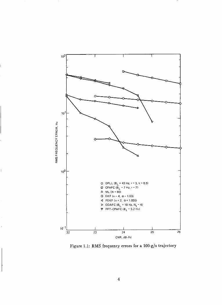
Figure 1.1 presents simulated rms frequency error as a function of CNR for the DPLL, MLE, FFT- CPAFC, EKF, ODAFC, FEKF, and CPAFC algorithms with 100-g/s jerk. RAJPO’s specification for maximum allowed rms error, 51.2 Hz (32 ft/s) at 28 and 35 dB-Hz and 50-g acceleration, is clearly met by all the algorithms evaluated. The conversion factor from ft/s to Hz is 1.6 Hz/(ft/s), based on the Doppler effect at GPS L1 frequency. All the algorithms simulated present virtually no loss-of-lock at 28 dB-Hz under the specified dynamics. One must note that RAJPO’s specification is for 50-g dynamics with unspecified dynamics before and after the maneuver, while our results are for the particular trajectory defined later.
Acquisition algorithms were evaluated for various dynamics. The critical dynamics parameter here is the maximum (unknown) velocity, which corresponds to the size of the frequency domain area that must be searched. Results show that RAJPO’s specifications, TTFF of 5.3 s at CNR of 28 dB-Hz and 3.9 s at 35 dB-Hz for dynamics of 6150 ft/s, are met by the two-dimensional search algorithm, and that the portion of TTFF allocated to channel acquisition can be reduced to less than 0.5 s. The part of TTFF that is allocated to settling of the navigation Kalman filter is not affected.
1.4 Conclusions and Recommendations
Results presented here show that the high-dynamics tracking algorithm implemented in the TPS meets all of RAJPO’s requirements. Other algorithms presented here provide improved perfor- mance in terms of both tracking and acquisition capabilities. These should be considered for implementation for future suitable applications.
3
102
10'
N I a'
a
t 0 2 W 3
a: U ln
s W
?I
z 1 oc
lo- '
0 DPLL ( B L = 43 Hz, r = 3, k z 0 . 5 ) 0 CPAFC (BL = 7 Hz, r = 2) A M L ( N = 8 0 ) 0 EKF (n = 4, Q = 1.03) a FEKF (n = 2, a = 1.005) D O D A F C ( B L = ~ O H Z , N ~ = ~ ) 0 FFT-CPAFC (BL = 5.2 Hz)
22 23 24 25 L
CNR. dB-Hz
Figure 1.1: RMS frequency errors for a lOO-g/s trajectory
4
Chapter 2
Purpose and Scope
2.1 Purpose
The purpose of this final report is t o document the GPS high-dynamic tracking concepts that have been developed under the task plan, to evaluate the performance of these methods, and to present performance comparisons between the different algorithms, including the FFT-CPAFC loop used in the TPS procurred by RAJPO. This report fulfills deliverable item (e) of JPL’s Task Plan RE-182, Amendment 452A, “High Dynamic GPS Range Instrumentation Receiver” [3], sponsored by the U.S. Air Force System Command, Armament Division.
2.2 Scope
This report documents the concepts, testing, results, and conclusions per the task plan. Chapter 3 presents a historical perspective of this task and a definition of the high-dynamic environment model used in the remainder of this report for both simulations and measurement. Chapter 4 briefly describes the various high-dynamic tracking algorithms developed at JPL and IEC. (Detailed algorithm descriptions are included in the references.) Chapter 5 describes the experimental setup used at JPL to evaluate real-time performance. Chapter 6 presents results of algorithm evaluation both in software simulations and using the experimental setup. Chapter 7 concludes this report by highlighting some of the significant results of this task.
5
Chapter 3
Introduct ion
3.1 History
JPL has pioneered the development of high-dynamic parameter estimation techniques for GPS receivers and related applications. This effort began in 1983 when JPL received a contract from RAJPO to validate a proposed concept for tracking high-dynamic vehicles without the use of inertial aiding. The problem arises because high dynamics introduce correspondingly high Doppler frequency shifts on the GPS RF carrier signals. When these Doppler shifts are large enough, the receiver’s PLL (actually a Costas loop) cannot maintain lock, and carrier tracking is lost. Since carrier tracking provides the navigation solution with accurate measurements of range rate, the quality of the range and velocity estimate is degraded. In addition, the loss of carrier tracking prevents recovery of the 50-Hz data modulation. The JPL concept was to apply an MLE approach to carrier frequency tracking, using an FFT processor. This approach allows for recovery of range and range rate estimates even in the presence of very high dynamics. Range can also be recovered from the code delay locked loop.
In 1984-85, JPL developed a breadboard single-channel simulation system and verified performance of this concept with actual hardware. The design was mostly digital so that a proposed receiver architecture was suitable to miniaturization using VLSI technology. Breadboard tests showed that both pseudorange and range rate could be tracked simultaneously in the presence of 50-g to 100-g accelerations at CNRs as low as 28 dB-Hz, without inertial aiding. These results were also confirmed via analyses and extensive simulations. Results of that work are documented in [2] and [4].
3.2 Outline of Completed Research
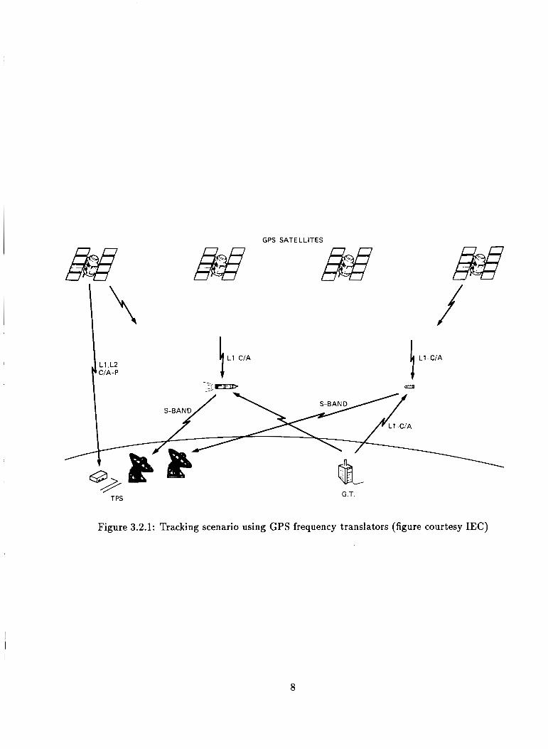
Subsequent JPL activity carried out under this task plan focused in two areas: tracking of high- dynamic GPS signals in the presence of data-wipe and tracking of BPSK-modulated signals. Data- wipe consists of the use of a secondary channel to remove the 50-Hz data modulation from the GPS signal. This can be performed in RAJPO’s environment when a translator is used (Figure
6
3.2.1). In this case, the high-dynamic vehicle carries a frequency translator that receives the GPS signals in L-band, translates them t o a different frequency band, and then transmits them to a ground station. The GPS signal is also received from the GPS satellites directly at the ground system and the 50-Hz data is recovered using a separate GPS receiver. The recovered 50-Hz data is then applied t o the re-transmitted signal (from the translator) with appropriate delay t o “wipe” the data modulation. This approach, if properly implemented, results in the reception of a Doppler unmodulated tone, rather than a harder-to-track BPSK-modulated sine wave. The second area of JPL’s work was improved tracking of BPSK-modulated signals using differential techniques.
Several frequency trackers were evaluated for the data-wipe case. These included extensions of the MLE concepts proven in the preceding task, a novel application of the EKF, ramifications of the CPAFC loop, and a DPLL. The fine tuning and performance of these frequency estimators were shown to depend on the signal dynamics, and were related to the maximum allowable observation time and highest-order derivative of the frequency process. Software simulations showed that both the MLE and the EKF can track trajectories that include 100-g/s jerk pulses with estimation errors of only a few Hertz at CNRs as low as 24 dB-Hz. In addition, the MLE maintained lock with 90 percent probability over this severe trajectory even at 23 dB-Hz.
After simulations of these algorithms were completed [5], several of these algorithms were demon- strated using a modified version of NASA’s Advanced Receiver breadboard as a testbed. As the Advanced Receiver breadboard was not originally designed for this purpose, several hardware and software modifications were required. These modifications are described in Chapter 5. The PLL, CPAFC, EKF and a hybrid algorithm developed by IEC, denoted an FFT-CPAFC algorithm, were implemented and tested on the breadboard, confirming the analyses and simulations.
In the second area, tracking of BPSK-modulated carriers, work was based on various ALS al- gorithms. These algorithms use optimal estimation techniques and are rather computationally intensive, but provide superior performance.
3.3 Definition Of High-Dynamic Trajectory
A fundamental question in developing techniques for the tracking of high-dynamic vehicles is “What are high dynamics?” Usually, one interprets this as high values for velocity and its derivatives. In the preceding task [2], two high-dynamic trajectories were used: one that simulated circular motion, or turns, the other simulating linear acceleration. In the first trajectory the velocity and its derivatives are sine waves, corresponding to motion in a circle with a period of 6 to 8 s, and with radial acceleration of 50 g. This trajectory exibits an infinite number of derivatives and is hard to track with an algorithm that assumes a polynomial model for the velocity. The second trajectory assumed that the acceleration is constant throughout, except for a step change of 50 g. Both trajectories represented hard-to-track environments.
In this task, the performance of the various estimators was evaluated on the basis of their ability to track a common trajectory. The trajectory chosen for both the simulation and the hardware demonstration experiments is derived from RAJPO’s specification (11 and uses step jerk (derivate of acceleration) as the most stressing dynamic. The FFT-CPAFC, used in the TPS, was evaluated
7
GPS SATELLITES
f
G.T. TPS
Figure 3.2.1: Tracking scenario using GPS frequency translators (figure courtesy IEC)
8
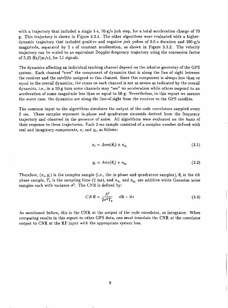
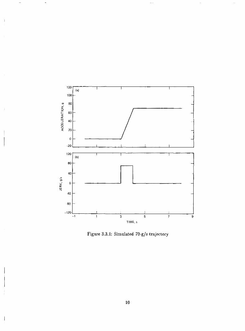
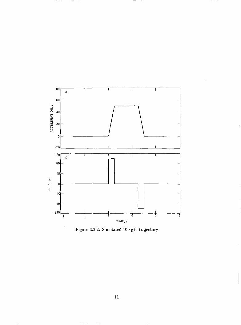
with a trajectory that included a single 1-s, 70-g/s jerk step, for a total acceleration change of 70 g. This trajectory is shown in Figure 3.3.1. The other algorithms were evaluated with a higher- dynamic trajectory that included positive and negative jerk pulses of 0.5-s duration and 100-g/s magnitude, separated by 2 s of constant acceleration, as shown in Figure 3.3.2. The velocity trajectory can be scaled to an equivalent Doppler-frequency trajectory using the conversion factor of 5.25 Hz/(m/s), for L1 signals.
The dynamics affecting an individual tracking channel depend on the relative geometry of the GPS system. Each channel “sees” the component of dynamics that is along the line of sight between the receiver and the satellite assigned to this channel. Since this component is always less than or equal to the overall dynamics, the stress on each channel is not as severe as indicated by the overall dynamics, i.e., in a 50-g turn some channels may “see” no acceleration while others respond to an acceleration of some magnitude less than or equal to 50 g. Nevertheless, in this report we assume the worst case: the dynamics are along the line-of-sight from the receiver to the GPS satellite.
The common input to the algorithms simulates the output of the code correlators sampled every 2 ms. These samples represent in-phase and quadrature sinusoids derived from the frequency trajectory and observed in the presence of noise. All algorithms were evaluated on the basis of their response to these trajectories. Each 2-ms sample consisted of a complex number defined with real and imaginary components, 2; and y;, as follows:
(3.2) y; = Asin(&) -+ nYi
Therefore, (xi, y;) is the complex sample (i.e., the in-phase and quadrature samples), 8; is the ith phase sample, T, is the sampling time (2 ms), and nZi and ny, are additive white Gaussian noise samples each with variance u2. The CNR is defined by:
dB - HZ A2 2u2T,
C N R = - (3.3)
As mentioned before, this is the CNR at the output of the code correlator, or integrator. When comparing results in this report to other GPS data, one must translate the CNR at the correlator output to CNR at the RF input with the appropriate system loss.
9
120
100
80 i 0 a I- (r W 1 w u 0 a
v) . m
J a W 7
(a) I I I I
-
-
120
80
-80 -401
I I I b)
I
-
120 I I I 1 I - 1 1 3 5 7 9
TIME, s
Figure 3.3.1: Simulated 70-g/s trajectory
10
80
60 m
120
80
40
-40
-80
40
20
0
-20
I 1 1 (b) c
- -
- -
0 - -
- -
- - L
- 1 1 3 5 7 9
TIME, s
Figure 3.3.2: Simulated 100-g/s trajectory
11
Chapter 4
Algorithm D escriptions
In this chapter, various tracking and acquisition algorithms are presented. Descriptions of most of the algorithms have already been published in the literature in one form or another, so no attempt is made here to reproduce the analysis. Instead, a brief description is given and the reader is directed to the appropriate publications for more detailed information. Algorithms are presented in three different categories. First, we present frequency tracking algorithms for data-wipe environments, i.e, MLE, EKF, DPLL, CPAFC, ODAFC, FEKF, and FFT-CPAFC. Then, algorithms for frequency tracking that apply ALS algorithms are presented. Finally, algorithms for fast initial acquisition of GPS signals are discussed.
4.1 Maximum Likelihood Estimator (MLE)
The structure and performance of the MLE of frequency in the presence of dynamics and additive noise is detailed in [5] . Here we present a brief description of the basic operations carried out by this estimator and summarize its performance by means of estimated rms estimation errors and estimated loss-of-lock probabilities.
The MLE bases its estimate of frequency (and its time derivatives) on a vector of N consecutive in-phase and quadrature samples. The estimator structure is based on the maximization of the likelihood function, derived from the conditional joint density of the observed samples, conditioned on the relevant signal parameters. It is shown in [5 ] that even for severe dynamics characterized by 100-g/s jerk pulses, it is sufficient to carry out the maximization of the likelihood function over the two-dimensional frequency-frequency rate plane, without incurring large estimation errors near the operating threshold. Thus, to first order, the effects of jerk (the rate of frequency rate) can often be ignored. However, the simultaneous estimation of both frequency and frequency rate is crucial, even though only the frequency estimates are of interest.
The maximum likelihood estimator can be implemented by evaluating the likelihood function over a grid of points in the frequency-frequency rate plane, with spacing fine enough to resolve the likeli- hood function near its peak. This implementation can be reduced to a sequence of FFTs performed
12
on a suitably weighted input sequence, where the complex weights depend on the frequency-rate coordinate. Rough estimates of frequency and frequency rate are simply the coordinates of the peak, which can be refined by means of interpolation algorithms as needed.
The simulation results are summarized in [5]. The rms estimation errors exhibit a well-defined threshold, below which a rapid increase in the estimation error occurs. This is also the region where loss-of-lock begins to be a problem (loss-of-lock is a condition in which the frequency estimates become independent of the true frequency). Here we define the loss-of-lock threshold as that CNR at which the estimator loses lock ten percent of the time. For N = 80 ( N is the number of samples used in the FFT before zero-padding), simulation results were also obtained using the true value of jerk, in order to bound the possible improvement in the frequency estimates and loss-of- lock performance if the jerk was estimated as well. Apparently, no improvement is possible near threshold. Above threshold, however, rms frequency estimation errors could be reduced by the simultaneous estimation of jerk, acceleration, and velocity components. With the given trajectory, a CNR threshold of 23 dB-Hz was achieved with N = 50, resulting in a 7-Hz rms error.
4.2 Extended Kalman Filter (EKF)
Kalman filters have been shown to be the optimum estimators when the received signals are lin- ear functions of the unknown parameters and are observed in the presence of Gaussian noise [6]. However, when the observables are nonlinear functions of the parameters, extended Kalman filters (EKF) are employed which basically linearize the functions locally around the current estimate. As a result, EKFs are not the optimum estimators in the absolute sense.
For the current application, both third- and fourth-order EKFs were analyzed and simulated. Unlike the MLE, the EKF provides frequency estimates every 2 ms rather than an averaged estimate. Additionally, both phase and frequency rate estimates are provided. The transient response of the EKF was improved by including an additional exponential coefficient to weight past data. For the given trajectory, weighting the past 40 samples was found to provide the best performance. The details of the equations are all included in [5] along with the performance curves for different filters and parameters. Frequency threshold attained by the fourth-order E K F is about 24 dB-Hz with a 3-Hz rms error. Although phase is of secondary importance in the current application, its threshold was only 0.5-dB higher at 24.5 dB-Hz with a 0.4-rad rms error.
4.3 Cross-Product AFC (CPAFC) Loop
A simple sub-optimal method of estimating the frequency of a sinusoidal signal embedded in noise and subject to severe dynamics is the CPAFC loop. Basically, frequency discrimination is obtained by employing a cross-product between the in-phase and quadrature signals, thus removing the phase. The error signal is then filtered and fed to a numerically controlled oscillator (NCO). Even though the CPAFC loop permits operation at low CNRs where a PLL is inoperative, it also increases the rms frequency error.
13
In the presence of time-varying Doppler, the loop bandwidth needs to be adjusted such that a balance is reached between noise immunity (obtained with small loop bandwidth) and dynamic tracking (typically requiring larger loop bandwidth). Both second- and third-order loop filters were tested for the given jerk [5]. A threshold of 24.7 dB-Hz was achieved with an 8-Hz loop bandwidth and second-order filter. However, the frequency estimation error was 31 Hz rms at 26- dB-Hz CNR. Using a third-order filter with loop bandwidth of 5.5 Hz can achieve a slightly lower threshold (approximately 0.3-dB lower) with almost no impact on rms frequency error.
4.4 Digital Phase-Locked Loop (DPLL)
Frequency estimation can be achieved with traditional DPLLs by processing the phase estimates. However, in regions where the DPLL is inoperative due to cycle slipping, no frequency information can be derived; hence, the frequency operation threshold is dominated by the phase behavior, which typically requires higher CNRs.
A type-I11 DPLL was simulated [5] and it was found that a nominal loop bandwidth of 43 Hz minimized the probability of loss-of-lock for our trajectory. A threshold around 26 dB-Hz was achieved with an rms frequency error on the order of 26 Hz.
4.5 Overlapping DFT AFC (ODAFC) Loop
Frequency discrimination can be achieved in several ways, one of which is to perform a simple cross-product between the in-phase and the quadrature signals as we have seen before. However, it is straightforward to show [7] that the cross-product is equivalent to a 2-point overlapping DFT.
A generalization would be to employ an N-point DFT where N can be optimized t o offer good noise reduction while tracking dynamics. In order to maintain the loop update rate at 2 ms, overlapping DFTs are used, offering better performance. Analysis and performance of this improved loop are presented in [7]. For the 100-g/s trajectory, a 4-point FFT implementation with 10-Hz loop achieves a 22.5-dB-Hz CNR threshold and rms frequency error of 17 Hz. Using an 8-point DFT and increasing the loop bandwidth to 14 Hz reduces rms frequency error t o 14 Hz with an increase in threshold CNR to 23 dB-Hz.
4.6 Frequency Extended Kalman Filter ( F E K F )
Tracking algorithms that ignore phase information appear to have a lower threshold CNR (as frequency trackers) than their counterparts that also estimate phase. This is certainly the case when comparing the DPLL and the CPAFC loop considered above. However, improvement in threshold CNR is achieved at the expense of degraded performance in terms of frequency rms error.
14
This situation provides the basis for the frequency EKF which performs a cross-product on the data in order to remove the phase. This modified set of data is then used in an EKF with a reduced order. This system can also be thought of as a CPAFC loop with an optimized loop filter. The analysis of such an algorithm is presented in [8] along with computer simulations. A second-order FEKF was able to achieve a 22.5-dB-Hz CNR threshold for the given trajectory with a 41-Hz rms frequency error. This certainly outperforms the CPAFC loop described earlier in terms of lowest
I
I operating CNR.
4.7 FFT-CPAFC LOOP
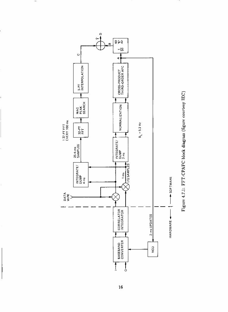
A block diagram of the CPAFC loop with FFT measurement correction as implemented by IEC is shown in Figure 4.7.1. This frequency estimator relies on a robust CPAFC loop to maintain lock, even in the presence of severe dynamics and additive noise. Although AFC loops can often maintain lock in extremely noisy environments, the rms estimation errors produced by these loops during dynamics are generally quite high. The central idea behind the IEC implementation is that if the instantaneous estimation errors could be estimated accurately and subsequently subtracted from the initial CPAFC estimates, then perhaps the total rms estimation error could be reduced. To this end, an FFT-based frequency estimator is employed to measure the residual error present in the in-phase and quadrature samples following the data-wipe operation, and prior to taking the cross-product. At this point, the 1-ms samples are converted to 2-ms samples within the CPAFC loop, and to 4-ms samples in the FFT estimator. Thus, the maximum frequency error possible within the CPAFC loop without loss-of-lock is f250 Hz, while the maximum range of the FFT estimator is f125 Hz. The output of the CPAFC drives the NCO, whose output closes the loop. An averaged version of the CPAFC output is also available every 100 ms for combining with the FFT estimates.
The FFT estimator operates as follows: every 100 ms, 25 4-ms samples are collected, 7 zeros appended, and a 32-point FFT performed. A sinusoidal component in the samples gives rise to an impulse in the FFT output near the proper frequency, with a resolution of roughly 8 Hz (250/32). Thus, the magnitude of the FFT is computed, and the frequency corresponding to the location of the peak declared to be a rough estimate of the AFC frequency error. A refined estimate is obtained by performing 3-point quadratic interpolation. This refined estimate is then combined with the averaged CPAFC loop estimate synchronously every 100 ms to obtain the final frequency estimate.
The perfomance of this hybrid frequency estimator has been evaluated by means of simulation, nonlinear analysis, and hardware experiments. The results of the hardware evaluation are presented in Section 6.1.4, while the simulation resuts and the analysis are presented in Appendix A.
15
N I
2 I1 1
m
V R
, P
16
4.8 Adaptive Least Squares (ALS)
Several algorithms were investigated under the collective title of Adaptive Least Squares. These algorithms are recursive in nature and require higher computational complexity than the previously described methods, but have potentially better performance. An ideal application for these algo- rithms is the post-mission processing of data. The following paragraphs describe these algorithms briefly, with more detailed descriptions in [9] and [lo].
4.8.1 Fast Frequency Acquisition
This algorithm provides for fast carrier acquisition in a data-wipe environment. The received signal is first demodulated by a carrier reference signal of known frequency and phase and by its 90-degree phase shifted version. The basic equations for the measurement express the noisy samples as a truncated (nth order) series involving the unknown frequency and phase, the sampling times, and the noise samples. The equations [9] are put in linear form involving a matrix of parameters that depends on the frequency and phase, and from which the frequency and phase can be determined.
The algorithm obtains the matrix of parameters from a sequence of N pairs of measurements using least squares estimation. This requires inversion of an N x N matrix that contains terms dependent on the sampling times and that can be precomputed and then multiplied by a matrix formed from the measurements. The matrix to be inverted has a specific structure that makes it possible to use a rapid algorithm for the solution. As a result, the desired matrix of parameters can be obtained in about 6Nlog2N operations, much fewer than the number of operations required for the “brute-force” calculations of a general matrix equation of similar form.
4.8.2 Differential Sampling for Fast Acquisition
This is an extension of the previous algorithm using a differential signal model along with appropri- ate sampling techniques. The algorithm is recursive in measurements and thus the computational requirements increase only linearly with the number of measurements.
The dimension of the state vector in the proposed algorithm does not depend on the number of measurements and is quite small, typically around four. This is an advantage compared to the previous algorithm where the dimension of the state vector increases monotonically with the product of frequency uncertainty and observation period. Further details are provided in [lo].
4.9 Signal Acquisition Algorithms
The initial acquisition of a GPS signal consists of two phases: first the individual tracking channels estimate pseudorange and range rate to the respective satellites, then, when sufficient channels
17
have acquired signals, a state (position, velocity, and time) solution is derived. Results presented here are concentrated on the first phase, channel acquisition.
The problem can be viewed as a twedimensional search, as shown in Figure 4.9.1. The unknown pseudorange is plotted on the horizontal axis, while the unknown range rate is plotted on the vertical axis. Pseudorange is obtained by searching for the appropriate C/A code lag that maximizes the code correlator output. Since the C/A code has 1023 lags, this search requires 1023 correlations with one-chip spacing or 2046 correlations with half-chip spacing. (The latter allows operation at lower CNR.) The search can be performed serially, i.e., sequential dwells for each possible code lag, using a single correlator, or in parallel, i.e., obtain all correlations during a single dwell by use of a bank of correlators. Parallel searching is feasible with today’s technology using VLSI. As an example, the TPS uses two VLSI chips to perform all 1023 correlations.
The second search is for range rate. Unknown range rate is due to two factors: uncertainty as to the center frequency, e.g., crystal frequency offset, and unknown Doppler due to the mutual dynamics of the vehicle and GPS satellite. Here also the search can be performed serially or in parallel. In the sequential search, used in the TPS, each step covers a frequency range that is inversely proportional t o the integration time. The TPS integration time is 1 ms, hence the frequency coverage of a single search step is approximately from -500 Hz to 500 Hz, with significant CNR degradation at higher frequencies. In each step of the serial search, the channel’s carrier NCO is positioned to a different center frequency so the search is for a range around that center frequency. In a parallel search, correlator outputs are sampled at a much higher rate and processed via FFT processors, hence a significantly higher frequency range can be covered. If total integration time remains fixed, then sampling the correlator output at 32 times per integration time will result in a searched frequency range that is 32 times larger than that covered by a serial frequency search. However, this improvement is at the cost of additional hardware complexity.
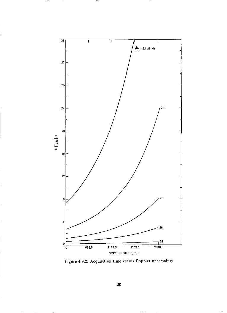
Algorithms for fully parallel searches are presented and analyzed in [ll] and [12]. A summary of results is presented in Figure 4.9.2. The figure illustrates channel acquisition time as function of Doppler uncertainty, for various CNR. We observe that for RAJPO’s specification of a Doppler uncertainty of 6150 ft/s and a CNR of 28 dB-Hz (using the 3-dB loss assumption), the channel acquisition time is less than 0.5 s. Even when adding the settling time of the navigation filter, this approach can save approximately 1 s from RAJPO’s TTFF specification.
The comparison of rms frequency error is somewhat unfair to the phase tracking algorithms. When the estimates are averaged over long time intervals, the rms frequency error becomes much better for the phase tracking algorithms. This is because the improvement is linear in time when phase tracking, but is proportional to the square root of time when not phase tracking.
4.10 Performance Comparison via Simulations
We conclude this chapter by comparing the different frequency tracking algorithms for the “data wipe” environment, using the trajectory described earlier in Section 3.3.
Table 4.1 summarizes the simulation results for the frequency tracking schemes. The comparison
18
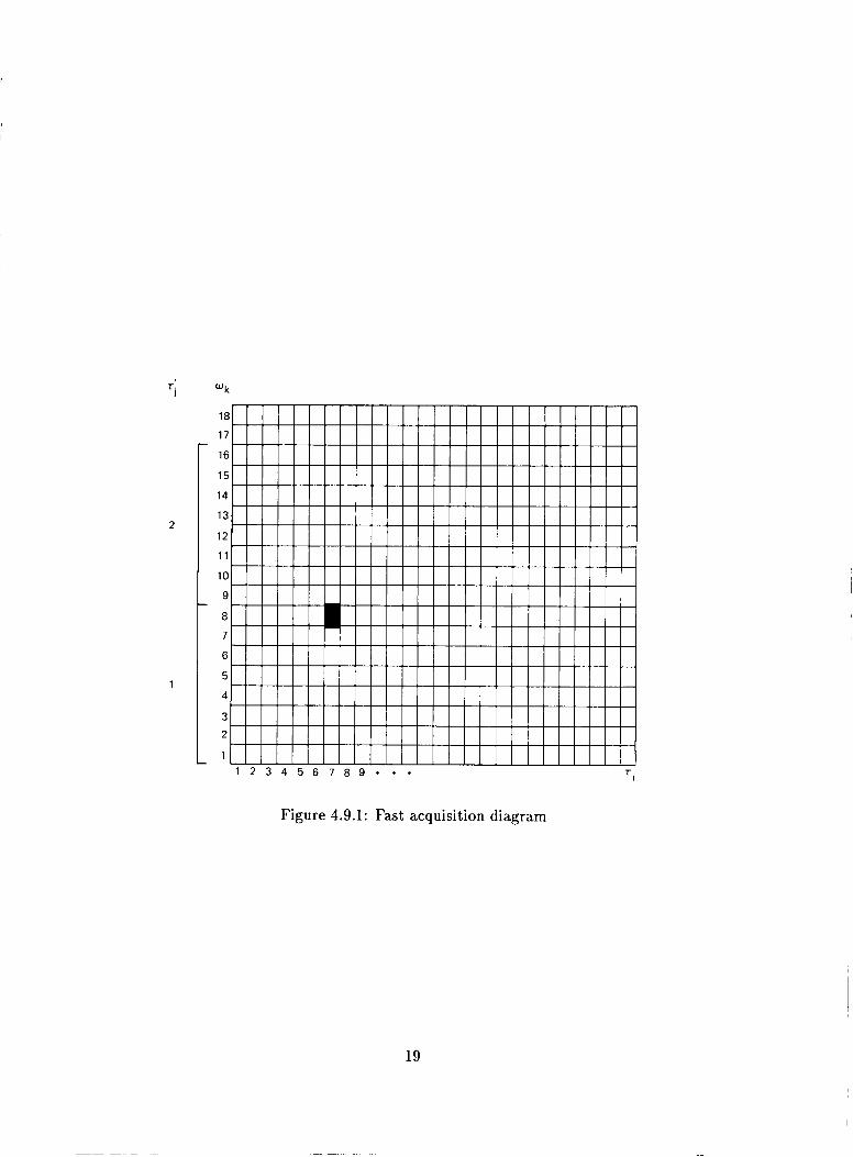
Figure 4.9.1: Fast acquisition diagram
19
36
32
28
1 6 = 23 dB-Hz
I I I S No = 23 dB-Hz
24 -
-
20 -
16 -
0 586.5 1 173.0 1759.5 2346.0
DOPPLER SHIFT, m/s
Figure 4.9.2: Acquisition time versus Doppler uncertainty
20
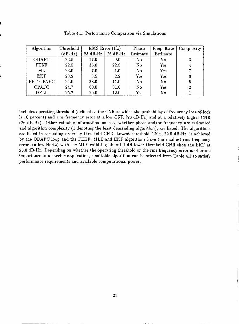
Table 4.1: Performance Comparison via Simulations
Phase Estimate
No N o No Yes No No Yes
ODAFC FEKF
ML EKF
CPAFC DPLL
FFT-CPAFC
Freq. Rate Estimate
N o Yes Yes Yes No Yes No
Threshold (dB-Hz)
22.5 22.5 23.0 23.9 24.0 24.7 25.7
23 dB-Hz 17.0 36.0 7.0 3.5
38.0 60.0 20.0
26 dB-Hz 9.0
22.5 1.0 2.2
11.0 31.0 12.0
includes operating threshold (defined as the CNR at which the probability of frequency loss-of-lock is 10 percent) and rms frequency error at a low CNR (23 dB-Hz) and at a relatively higher CNR (26 dB-Hz). Other valuable information, such as whether phase and/or frequency are estimated and algorithm complexity (1 denoting the least demanding algorithm), are listed. The algorithms are listed in ascending order by threshold CNR. Lowest threshold CNR, 22.5 dB-Hz, is achieved by the ODAFC loop and the FEKF. MLE and EKF algorithms have the smallest rms frequency errors (a few Hertz) with the MLE exibiting almost l-dB lower threshold CNR than the EKF at 23.0 dB-Hz. Depending on whether the operating threshold or the rms frequency error is of prime importance in a specific application, a suitable algorithm can be selected from Table 4.1 t o satisfy performance requirements and available computational power.
21
Chapter 5
Description of Experimental Se tup
The setup of the GPS high-dynamic receiver is considered and presented in this chapter. The breadboard Advanced Receiver (ARX) is described first since it constitutes the testbed for the GPS demonstration. Software as well as hardware modifications to the ARX are then discussed with emphasis on signal generation, as the latter contains the dynamics of interest.
The ARX is used as a testbed because it represents hardware typical of modern GPS receivers, specifically the TPS. The ARX obtains digital I and Q samples at a high rate (5 MHz for the ARX versus 2 MHz for the TPS), integrates the samples to reduce the data rate (1-ms integration for the TPS versus variable integration time in the ARX), and performs most of the remaining pro- cessing in software (Intel 80286 in the ARX versus Motorola 68000 in the TPS). Hence, algorithms demonstrated on the ARX have practical application to the TPS.
5.1 Advanced Receiver Block Diagram
The ARX is a hybrid analog/digital receiver which has been designed for use in NASA’s Deep Space Network (DSN). It uses intermediate frequency sampling and DPLL’s to perform carrier tracking, subcarrier tracking, and symbol synchronization [13].
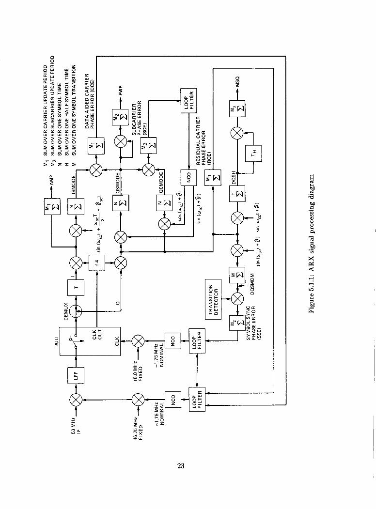
Figure 5.1.1 shows the ARX signal processing diagram. The receiver uses the open loop IF signal at 53 MHz from the RF front end. This signal is then passed through a total power automatic gain control (AGC) circuit before entering the carrier loop. The reference signal is produced by mixing a constant 46.25-MHz signal with the output of the carrier NCO (nominal 1.875 MHz) frequency. The output from this mixing passes through a lowpass filter and is digitized. The clock driving the A/D is derived from the symbol synchronization loop NCO and has a nominal value of 19.75 MHz. This technique ensures a fixed number of samples per symbol when the signal is BPSK modulated. The digitized 5-MHz signal (sampled at roughly 20 MHz) is then split into in-phase and quadrature components (each with a 10-MHz rate). Conversion to baseband is accomplished digitally using a 5-MHz signal phase locked to the sampling clock. The 10-MHz rates are then lowered to the
22
I
1
X 3
E D r
If q
rN w
I I-
IC
n
Iw <Q +
+-
- Y
a z ~
a w
-4- A
23
appropriate loop update rates using digital accumulators to perform carrier tracking, subcarrier tracking, and symbol synchronization. The various loop filters can also be set independently in software with different parameters, including loop order and loop bandwidth.
5.2 Modifications t o the ARX
In the current application, the received signal consists of a pure sine wave with a time-varying frequency driven by the prescribed trajectory. The amplitude of the tone is set such that the required CNR is achieved with fixed noise power. Subcarrier and symbol synchronization are not used since they are not required for tracking the frequency of an unmodulated tone.
The required software modifications constituted a significant part of the work, which included algorithm implementation, system programming, and performance evaluation. Hardware changes were required mainly in the signal generation subsystem for the purpose of generating the dynamics.
5.2.1 H a r d w a r e Modifications
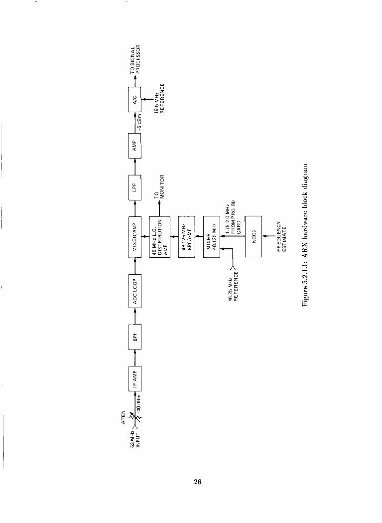
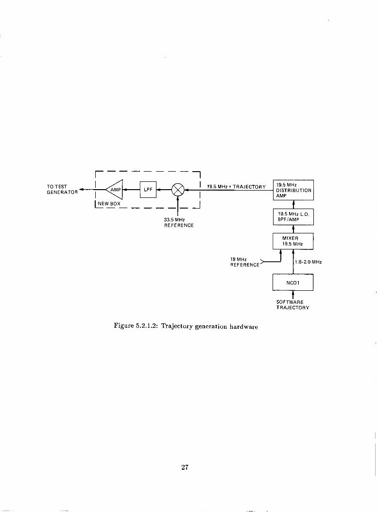
Modifications in the system’s hardware were essential due to the nature of the experiment. The A/D clock was set to a fixed 19.5 MHz derived directly from a frequency synthesizer. As for the signal generation, the software-generated trajectory was driving an NCO with a 1.5-MHz nominal frequency, its output was mixed with a fixed 18-MHz reference, band-pass filtered, and then up- converted again to 53 MHz using a fixed 33.52-MHz reference. The center frequency of 53.02 MHz was chosen to avoid a bias observed at 53 MHz. This bias will later be described and characterized in more detail. The new configuration is depicted in Figure 5.2.1.1 with the signal generation path shown in Figure 5.2.1.2.
5.2.2 Software Modifications
The Advanced Receiver software program (ARX) is a menu-driven system that allows the operator to set parameters such as bandwidth, symbol-to-noise ratio (SNR), carrier and subcarrier update rates, etc. It also allows the operator to choose from several possible displays for the CRT monitor and, upon operator request, will log statistical data on a disk. The ARX, upon request, performs either preacquisition or tracking.
The ARX is divided into sixteen sections called modules. Eight of these sixteen modules had to be modified to accommodate the differences in the requirements of the ARX and the Global Positioning Satellite (GPS) demonstration. The eight modules that needed modification are:
1. ADRCF-the foreground module that acquires the in-phase and quadrature (I and Q) samples from the A/D convertors, solves the loop filter equations, drives the NCO (see Figure 5.2.1.1) and acquires data for displaying or logging.
24
2. ARPRINT-the background module that performs the data reduction, writes to the CRT monitor and logs to the disk.
3. ARFAST-the module that performs all of the communication with the array processor board (AP-4) for FFT processing as part of frequency error estimation.
4. ARPCALC-the module that calculates all of the parameters necessary to initialize the hard- ware (i.e., the count registers that control I and Q update rates), the loop filter coefficients, and the gains and constants needed for data reduction.
5. ARINITL-the module that sets the default values to parameters and clears memory areas where required.
6. ARPENTR-the module that accepts and translates the operator inputs for setting param- eters and controlling the execution of the software.
7. ARMENUS-the module with the monitor displays of the menus.
8. ARGLOB-the insert module that defines all of the globally used parameters.
The changes to each of the eight modules of the ARX to effectively simulate the GPS are described in Appendix C.
25
0
0 $ 5 H E -.- a
0 Ncp
m U
Y
26
a H a
a z E + W
a
x I
,
I 19.5 MHz +TRAJECTORY LPF
I I TO TEST I GENERATOR
Figure 5.2.1.2: Trajectory generation hardware
19.5 MHz D ISTR I BUT ION AMP
27
NEW BOX L - - - - - - t 19.5 MHz L.O.
_I - 33.5 MHz REF E RENCE
B P FIAM P
t MIXER 19.5 MHz
R E F E RENCE'
~
Chapter 6
Algorithm Evaluation
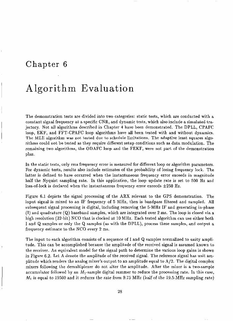
The demonstration tests are divided into two categories: static tests, which are conducted with a constant signal frequency at a specific CNR, and dynamic tests, which also include a simulated tra- jectory. Not all algorithms described in Chapter 4 have been demonstrated. The DPLL, CPAFC loop, EKF, and FFT-CPAFC loop algorithms have all been tested with and without dynamics. The MLE algorithm was not tested due to schedule limitations. The adaptive least squares algo- rithms could not be tested as they require different setup conditions such as data modulation. The remaining two algorithms, the ODAFC loop and the FEKF, were not part of the demonstration plan.
In the static tests, only rms frequency error is measured for different loop or algorithm parameters. For dynamic tests, results also include estimates of the probability of losing frequency lock. The latter is defined to have occurred when the instantaneous frequency error exceeds in magnitude half the Nyquist sampling rate. In this application, the loop update rate is set to 500 Hz and loss-of-lock is declared when the instantaneous frequency error exceeds f 2 5 0 Hz.
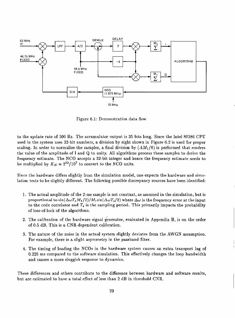
Figure 6.1 depicts the signal processing of the ARX relevant to the GPS demonstration. The input signal is mixed to an IF frequency of 5 MHz, then is bandpass filtered and sampled. All subsequent signal processing is digital, including removing the 5-MHz IF and generating in-phase (I) and quadrature (Q) baseband samples, which are integrated over 2 ms. The loop is closed via a high resolution (32-bit) NCO that is clocked at 10 MHz. Each tested algorithm can use either both I and Q samples or only the Q samples (as with the DPLL), process these samples, and output a frequency estimate to the NCO every 2 ms.
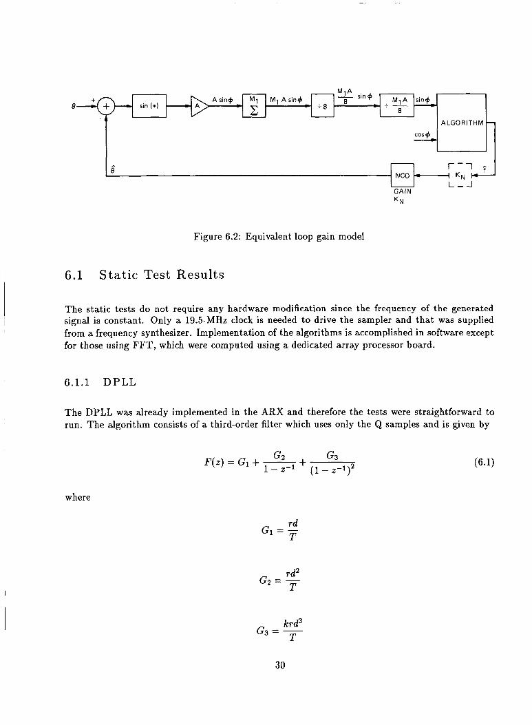
The input to each algorithm consists of a sequence of I and Q samples normalized to unity ampli- tude. This can be accomplished because the amplitude of the received signal is assumed known to the receiver. An equivalent model for the signal path to determine the various loop gains is shown in Figure 6.2. Let A denote the amplitude of the received signal. The reference signal has unit am- plitude which renders the analog mixer’s output to an amplitude equal to A/2. The digital complex mixers following the demultiplexer do not alter the amplitude. After the mixer is a twesample accumulator followed by an MI-sample digital summer to reduce the processing rate. In this case, MI is equal to 19500 and it reduces the rate from 9.75 MHz (half of the 19.5-MHz sampling rate)
28
IF
LPF - AID T t - p - 3 - A
46.25 MHz FIXED
1 ) I 1 c - 4
19.5 MHz FIXED
v
Figure 6.1: Demonstration data flow
ALGORITHM
to the update rate of 500 Hz. The accumulator output is 35 bits long. Since the Intel 80286 CPU used in the system uses 32-bit numbers, a division by eight shown in Figure 6.2 is used for proper scaling. In order t o normalize the samples, a final division by ( A M 1 / 8 ) is performed that renders the value of the amplitude of I and Q to unity. All algorithms process these samples to derive the frequency estimate. The NCO accepts a 32-bit integer and hence the frequency estimate needs to be multiplied by K N = 232/107 to convert to the NCO units.
Since the hardware differs slightly from the simulation model, one expects the hardware and simu- lation tests t o be slightly different. The following possible discrepancy sources have been identified:
1. The actual amplitude of the 2-ms sample is not constant, as assumed in the simulation, but is proportional to sin(AwT,M~/2)/M~sin(AwT,/2) where ALJ is the frequency error at the input to the code correlator and T, is the sampling period. This primarily impacts the probability of loss-of-lock of the algorithms.
/ 2. The calibration of the hardware signal generator, evaluated in Appendix B, is on the order
of 0.5 dB. This is a CNR-dependent calibration.
3. The nature of the noise in the actual system slightly deviates from the AWGN assumption. For example, there is a slight asymmetry in the passband filter.
4. The timing of loading the NCOs in the hardware system causes an extra transport lag of 0.225 ms compared to the software simulation. This effectively changes the loop bandwidth and causes a more sluggish response to dynamics.
These differences and others contribute to the difference between hardware and software results, but are estimated to have a total effect of less than 2 dB in threshold CNR.
29
Asin+ M i MI A sin+ 8 8
C t8 c ; cos + - ALGORITHM -
Figure 6.2: Equivalent loop gain model
4 e
6.1 S ta t ic Test Results
r - i 4 KN NCO 4
L L-J
The static tests do not require any hardware modification since the frequency of the generated signal is constant. Only a 19.5-MHz clock is needed to drive the sampler and that was supplied from a frequency synthesizer. Implementation of the algorithms is accomplished in software except for those using FFT, which were computed using a dedicated array processor board.
6.1.1 D P L L
The DPLL was already implemented in the ARX and therefore the tests were straightforward to run. The algorithm consists of a third-order filter which uses only the Q samples and is given by
where
rd G1 = - T
krd3 G3 = - T
30
2c
15
$ Le
a
> Ly
p 10
s z
Y 3
Le LL v)
5
0
I I I
PLL (STATIC TESTS) THIRD-ORDER LOOP ( r = 3, k = 0.5) - SIMULATION POINTS \ 3 0 MEASURED POINTS
-20 . I 1 I
25 30 35 40 45 , CNR, dB-Hz
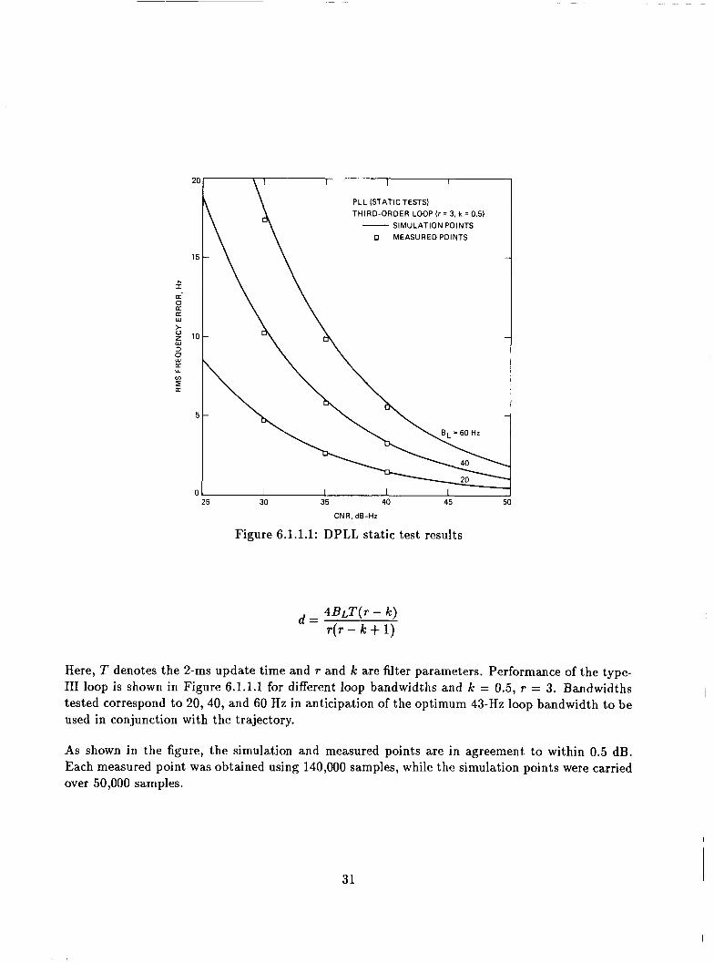
Figure 6.1.1.1: DPLL static test results
4B#( T - k) d = T ( T - k + 1)
Here, T denotes the 2-ms update time and T and k are filter parameters. Performance of the type- 111 loop is shown in Figure 6.1.1.1 for different loop bandwidths and k = 0.5, T = 3. Bandwidths tested correspond to 20,40, and 60 Hz in anticipation of the optimum 43-Hz loop bandwidth to be used in conjunction with the trajectory.
As shown in the figure, the simulation and measured points are in agreement to within 0.5 dB. Each measured point was obtained using 140,000 samples, while the simulation points were carried over 50,000 samples.
31
6 . 1 . 2 CPAFC
The CPAFC frequency discriminator uses both the I and Q samples in tracking the received fre- quency. The discriminator output is represented by
V ( k ) = I(k - 1 ) Q ( k ) - Q ( k - l ) I ( k )
where k denotes discrete time. This is followed by a filter with transfer function
G2 F ( z ) = - G1 + 1 - z-1 (1 - z-1)2
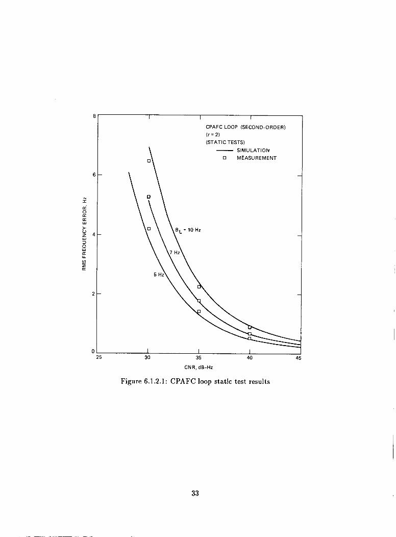
where G1 and G2 were given previously. Test results are shown in Figure 6.1.2.1 for a second-order loop ( T = 2) with an update rate of 500 Hz. The bandwidths tested correspond to 5, 7, and 10 Hz in anticipation of the optimum 7.5-Hz loop bandwidth to be used in conjunction with the trajectory.
As shown in Figure 6.1.2.1, simulation and measured points are in agreement to within 0.5 dB. Each measured point was obtained using 200,000 samples while the simulation points were carried over 500,000 samples.
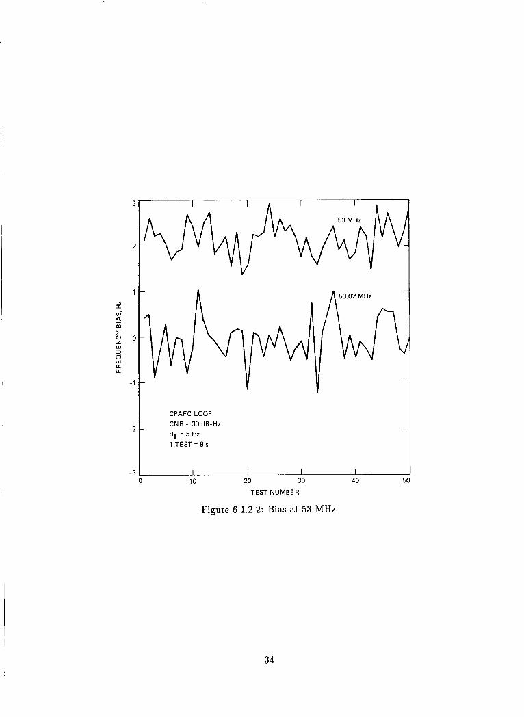
The tests were carried out at 53.02 MHz, a 20-kHz deviation from the nominal center. The deviation was necessary to reduce the effects of a bias, nonzero mean frequency error, encountered at 53 MHz. The cause of the bias has not been determined, but the bias was both CNR and center frequency dependent. Figure 6.1.2.2 depicts the bias at CNR = 30 dB-Hz for a 5-Hz loop bandwidth for both 53- and 53.02-MHz center frequencies. As shown, the estimation error is biased at 53 MHz, and for all practical purposes, unbiased at 53.02 MHz.
6 . 1 . 3 EKF
The EKF was implemented with steady-state gains to reduce the computational burden of com- puting and updating several vectors and matrices. For a fourth-order filter, the algorithm is given by
32
I I I
CPAFC LOOP (SECOND-ORDER) (r = 2) (STATIC TESTS)
SI MU LAT ION 0 MEASUREMENT
I 1 I > 30 35 40
CNR, dB-HZ
Figure 6.1.2.1: CPAFC loop static test results
33
3
2
1 N I vi 4 m > 0 0 2 3 W
2 [r U
-1
-2
-3
CPAFC LOOP CNR = 30 dB-Hz 8 ~ ~ 5 HZ 1 TEST = 8 s
I I I I 0 10 20 30 40
TEST NUMBER
Figure 6.1.2.2: Bias at 53 MHz
34
where p(k ) is the quadrature sample normalized by F a . The frequency fed to the NCO is derived from g( k) as
where k1, k2, k3, and k4 constitute the first column of the steady-state error covariance matrix given in [8]. Setting k4 to zero results in a third-order filter. It is worthwhile noting that the
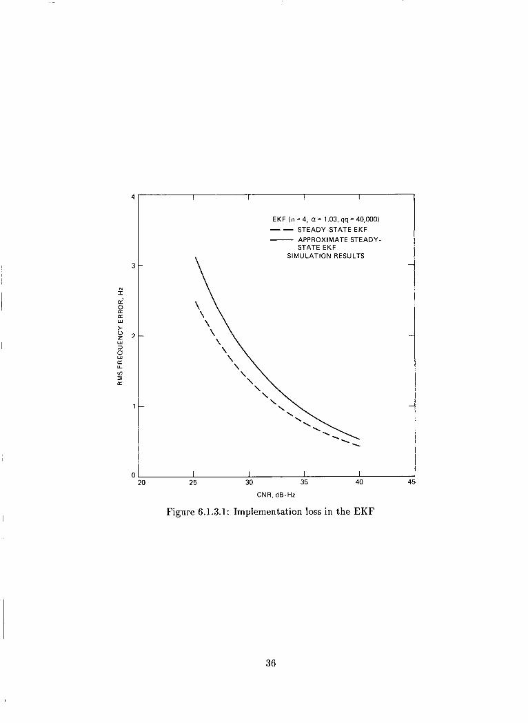
implementation corresponds to an approximation of the steady-state EKF in the sense that the signal controlling the NCO was set to be the difference between two consecutive phase estimates, whereas strictly speaking, the EKF requires mixing the received I and Q samples with an exact phase. The loss due to that approximation is shown in Figure 6.1.3.1 and is about 1.7 dB. For that reason, the measured threshold in the presence of dynamics will be at least 1.7 dB worse than previously predicted in [8].
-
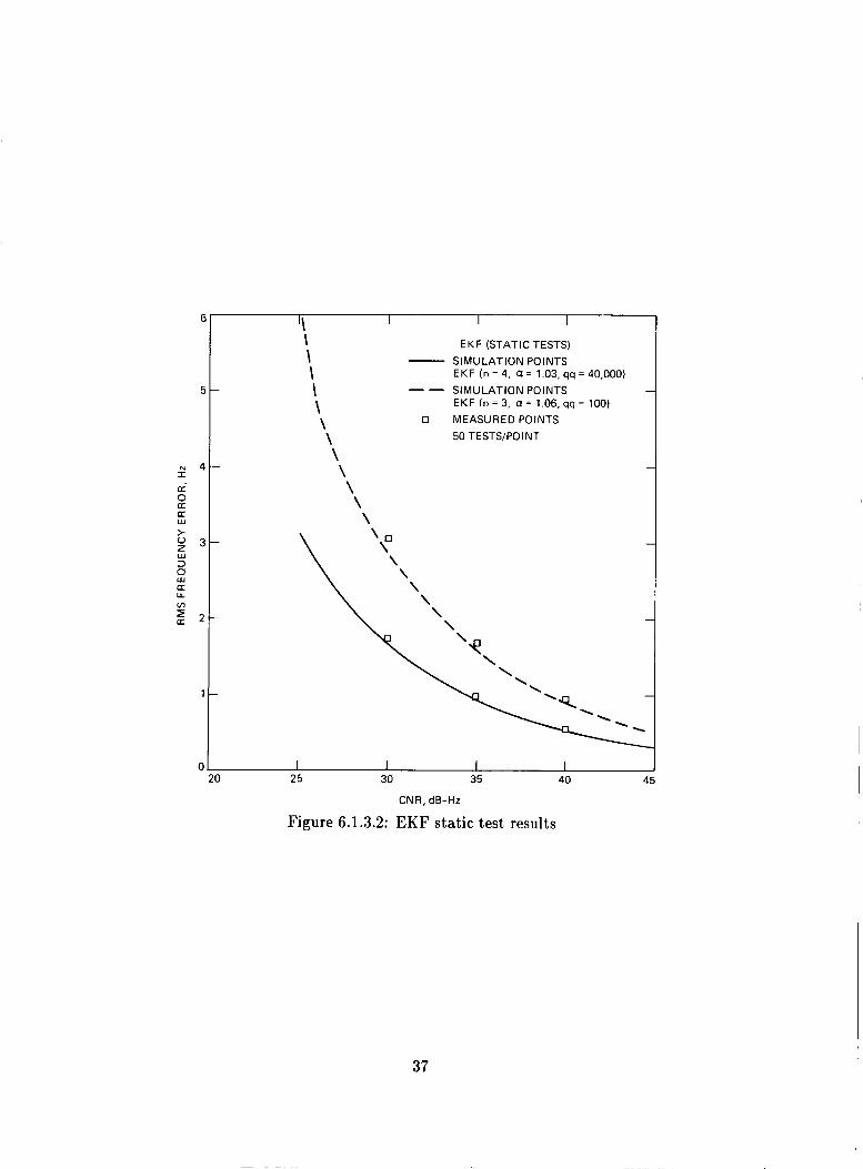
In Figure 6.1.3.2, the simulation and measured points are compared for both filter orders and are found to be in agreement. The phase, frequency, frequency rate, and the derivative of the frequency rate are given by z l ( k ) , 52(k) , ~ ( k ) , and z 4 ( k ) , respectively in units of rad, rad/s, etc.
6.1.4 FFT-CPAFC
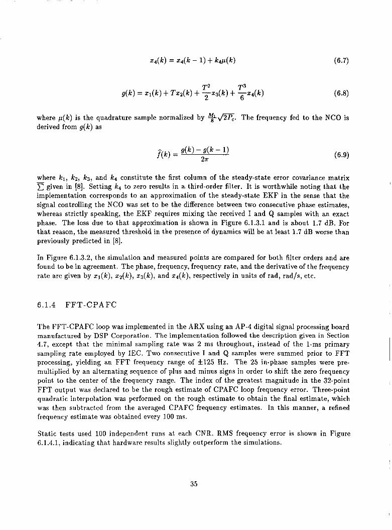
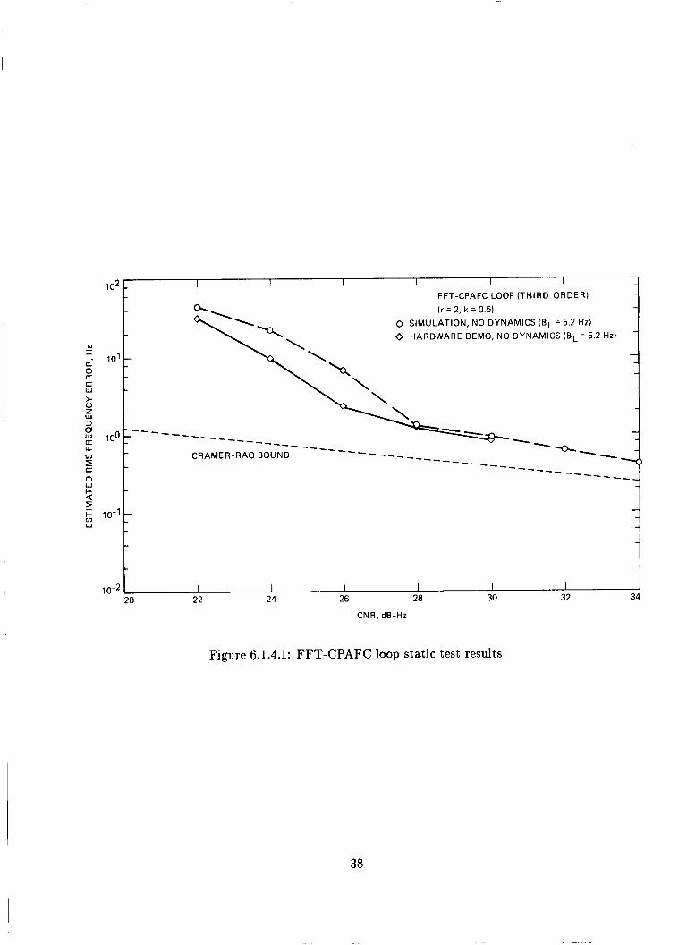
The FFT-CPAFC loop was implemented in the ARX using an AP-4 digital signal processing board manufactured by DSP Corporation. The implementation followed the description given in Section 4.7, except that the minimal sampling rate was 2 ms throughout, instead of the l-ms primary sampling rate employed by IEC. Two consecutive I and Q samples were summed prior to FFT processing, yielding an FFT frequency range of f 1 2 5 Hz. The 25 in-phase samples were pre- multiplied by an alternating sequence of plus and minus signs in order to shift the zero frequency point to the center of the frequency range. The index of the greatest magnitude in the 32-point FFT output was declared to be the rough estimate of CPAFC loop frequency error. Three-point quadratic interpolation was performed on the rough estimate to obtain the final estimate, which was then subtracted from the averaged CPAFC frequency estimates. In this manner, a refined frequency estimate was obtained every 100 ms.
Static tests used 100 independent runs at each CNR. RMS frequency error is shown in Figure 6.1.4.1, indicating that hardware results slightly outperform the simulations.
35
I I I I
EKF (n = 4, CI = 1.03, qq = 40,000) -- STEADY -STATE E K F
- APPROXIMATE STEADY- STATE EKF
SI MU LAT ION R ESU LTS
I I I I 3 25 30 35 40 45
CNR, dB-Hz
36
E
E
N 4
a'
a
I
s
g 3 z 5 2
w t
w 3
a U v)
1
0
I I\ \ \ \ \ \ \ \ \ \ \ \
I I
EKF (STATIC TESTS) S IMU LAT ION PO I NTS EKF (n = 4, Q = 1.03, qq = 40,000)
SI M U LATlO N PO I NTS EKF ( n = 3, Q = 1.06, qq = 100)
- -- 0 MEASURED POINTS
50 TESTS/POINT
I I 1 I 20 25 30 35 40 45
CNR, dB-HZ
Figure 6.1.3.2: EKF static test results
37
N r a
a w
t,
2
z
z w 3
a U v)
D w I- a E I- v)
w
Fimire 6.1.4.1: FFT-CPAFC ~ O O D static test results
38
6.2 Dynamic Test Results
Generation of the trajectory for the dynamic tests was accomplished by coding in software a subrou- tine that generates the frequency of the Doppler at 2-ms intervals, adds it to the 1.5-MHz nominal frequency of NCOl (Figure 5.2.1.1), converts it t o a 32-bit integer, and finally outputs it to the NCO. The test trajectory is described in Chapter 3.
6.2.1 D P L L
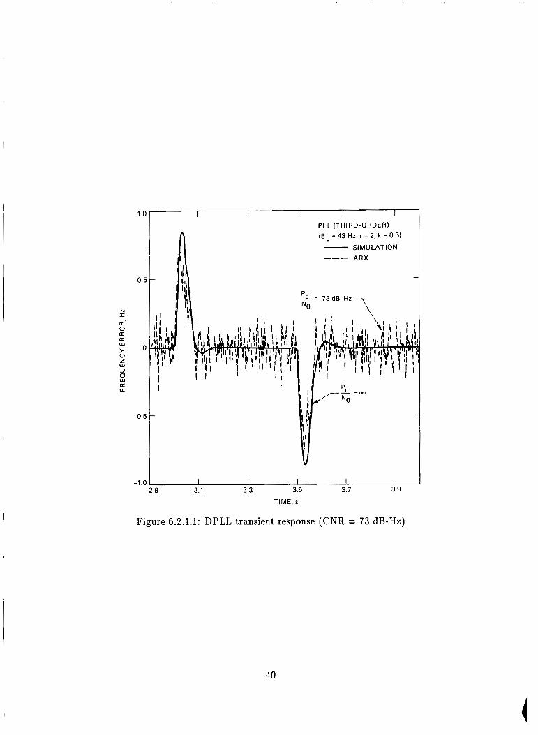
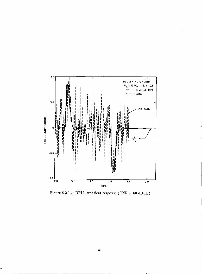
DPLL dynamic tests were conducted for different CNRs, using a 43-Hz loop bandwidth. Results are shown in the attached figures for a third-order loop with an update rate of 500 Hz ( B L = 43 Hz, r = 2, k = 0.5).
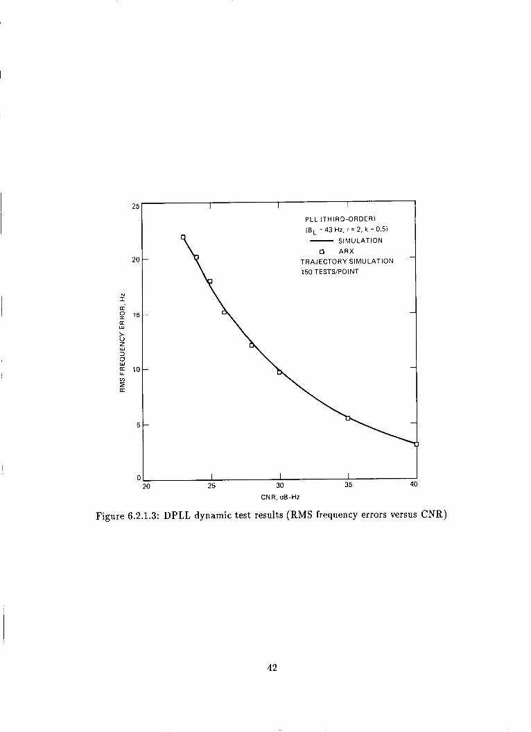
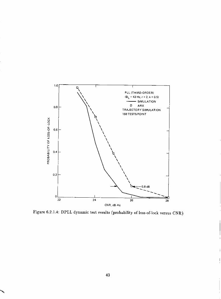
Transient frequency error versus time is plotted at very high CNR (73 dB-Hz in Figure 6.2.1.1 and 60 dB-Hz in Figure 6.2.1.2), showing steady-state error due to jerk at about 0.8 Hz. Measurement data are in agreement with the simulations (carried out without any noise) shown in solid line. Measured and simulated frequency rms error and probability of loss-of-lock are shown in Figures 6.2.1.3 and 6.2.1.4 versus CNR. The measured threshold (CNR at which frequency looses lock with 0.1 probability) occurred at 26 dB-Hz, while the simulated threshold occured at 25 dB-Hz. As for the rms values, they are in agreement to within 0.8 dB, as shown in Figure 6.2.1.3.
6.2.2 C P A F C
Tests were run with a second-order filter using an 8-Hz loop bandwidth and T = 2. For the given trajectory and filter, these parameters were found by simulation to minimize the CNR at which loss-of-lock occurred with a 10 percent probability.
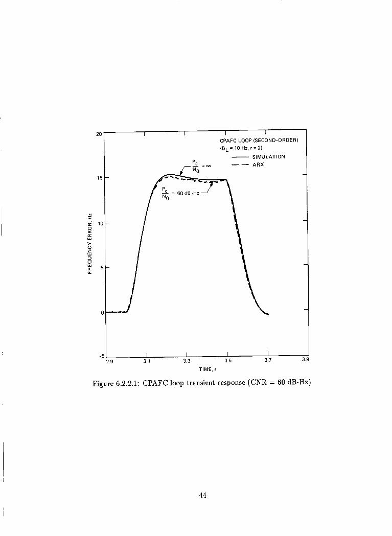
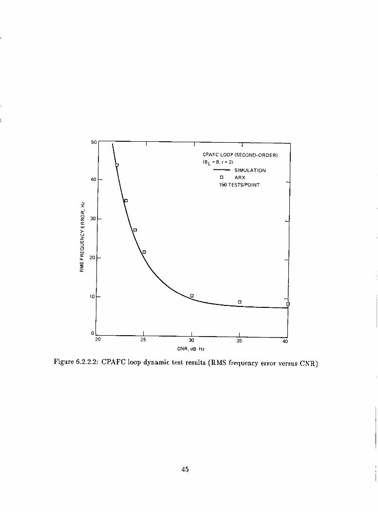
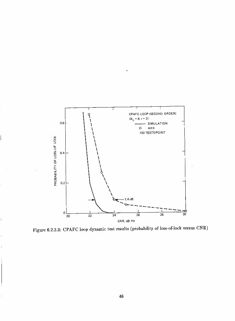
Figure 6.2.2.1 presents transient frequency error versus time at very high CNR (60 dB-Hz) to show the steady-state error due to jerk, which is about 14.5 Hz. Measurement and simulation data are in close agreement. Frequency rms error and the probability of loss-of-lock versus CNR are shown in Figures 6.2.2.2 and 6.2.2.3, respectively. Measured rms error is in close agreement with the simulations but the measured threshold is about 1.4 dB higher at roughly 24 dB-Hz.
6.2.3 E K F
Both the third- and fourth-order EKFs were tested in the presence of dynamics (the fourth-order EKF has been shown by simulation to possess a lower CNR threshold).
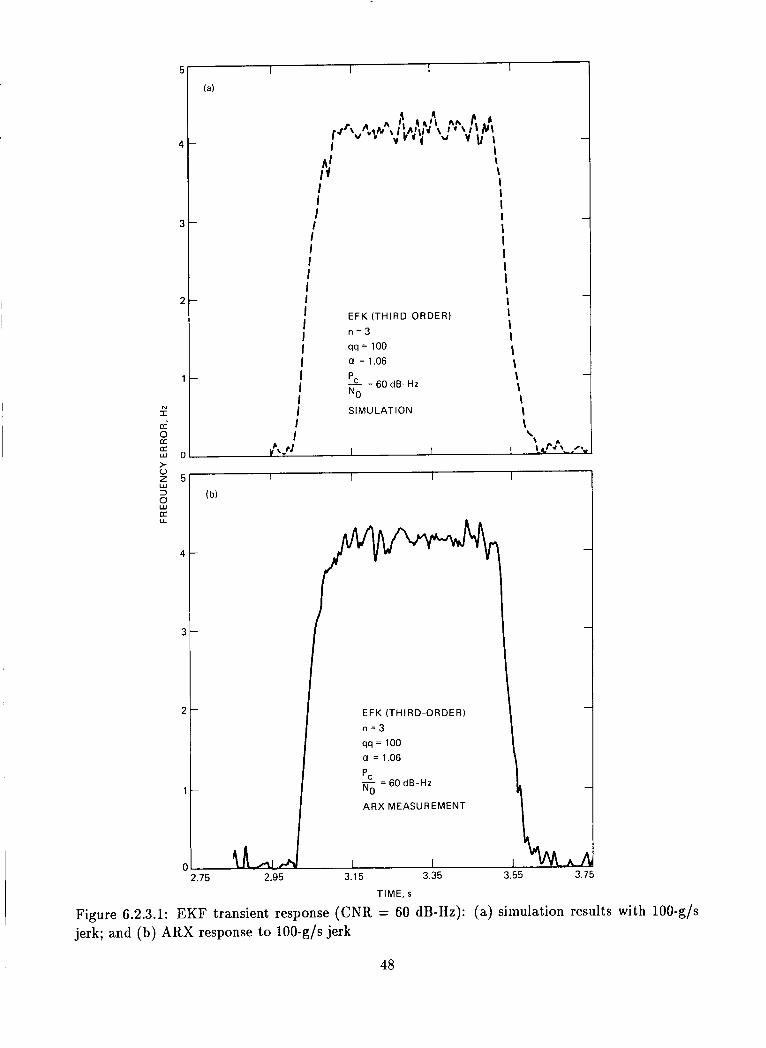
Figure 6.2.3.1 shows frequency error versus time at 60 dB-Hz, with maximum error due to jerk of 4.2 Hz for a third-order EKF. The measured points agree well with the simulations (also carried out at 60 dB-Hz) shown in dotted line. Frequency rms error and the probability of loss-of-lock
39
N I n 0 a a w > 0 Z
3 w
El a U
1 .o
0.5
0
-0.5
-1.c
I I I I I I
n PLL (THIRDORDER) (BL = 43 Hz, r = 2, k = 0.5)
I \ - SIMULATION I
11
t’ I
I I I I I .9 3.1 3.3 3.5 3.7 3.9
TIME, s
Figure 6.2.1.1: DPLL transient response (CNR = 73 dB-Hz)
40
N I a-
a w > 0 z w 3
x
E a U
I I I I PLL (THIRD-ORDER) (BL = 43 Hz, r = 2, k = C.5)
1 .o
SIMULATION - I ARX --- I " I
I ! I 1
I
I I I
I -1.01 I I I I I
2.9 3.1 3.3 3.5 3.7 3.9 TIME, s
Figure 6.2.1.2: DPLL transient response (CNR = 60 dB-Hz)
41
'.,
25
20
N I a'
15 a: w t 0 2 w 3
2 a 10
H U v)
a:
5
C
I I I PLL (THIRD-ORDER)
(EL = 43 Hz, r = 2, k = 0.5) - SIMULATION 0 ARX
TRAJECTORY SI MU LATlON 150 TESTS/POINT
I I I 0 25 30 35
CNR, dB-Hz
I
Figure 6.2.1.3: DPLL dynamic test results (RMS frequency errors versus CNR)
42
1 .I
0.f
Y 0 s + 0.f v) v)
3 U. 0 >- k J
0.4 Q m 0 n n
0.2
0
I 9 PLL (TH I RD-OR DE R ) (BL = 43 Hz, r = 2, k = 0.5)
SIMULATION - 0 ARX
TRAJECTORY SI MU LAT ION 150 TESTS/POINT
\ ' \
CNR, dB-Hz
Figure 6.2.1.4: DPLL dynamic test results (probability of loss-of-lock versus CNR)
43
I I I I CPAFC LOOP (SECOND-ORDER) (EL = 10 Hz, r = 2)
- SIMULATION ARX --
I I I I .9 3.1 3.3 3.5 3.7
TIME, s
Figure 6.2.2.1: CPAFC loop transient response (CNR = 60 dB-Hz)
44
51
4(
N I a'
a
> 0 Z
3
g 3( W
W
t ," 20 v) 5 a
10
0
I I
CPAFC LOOP (SECOND-ORDER) (EL = 8. r = 2) - S IMU LATl ON
0 ARX 150 TESTS/POINT - -
Figure 6.2.2.2: CPAFC loop dynamic test results (RMS frequency error versus CNR)
45
0.6
Y 0 s 4 s U
% 0.4
U 0 > k m J - 2 x 0.; a
(
CPAFC LOOP (SECOND-ORDE R )
(EL = 8, r = 2) - SIMULATION 0 ARX 150 TESTYPOINT
-3, G 1 . 4 d B -\
I I I I --- --- ----- --
22 24 26 28 20
I
CNR, dB-HZ
Figure 6.2.2.3: CPAFC loop dynamic test results (probability of loss-of-lock versus CNR)
46
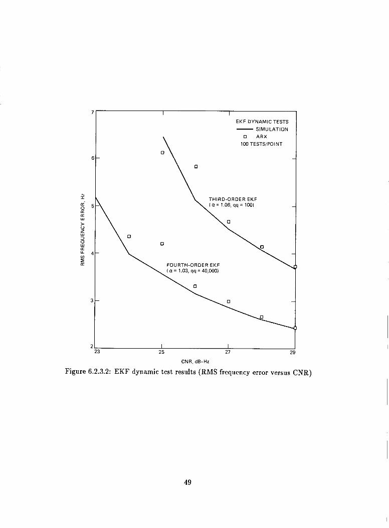
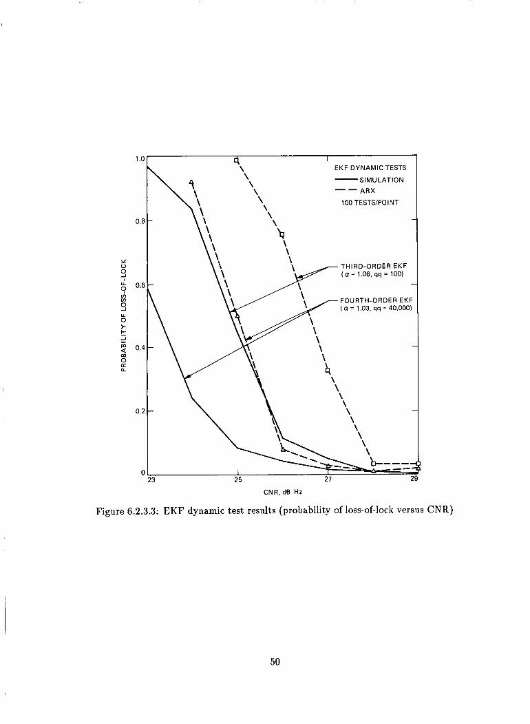
versus CNR are shown in Figures 6.2.3.2 and 6.2.3.3. The measured rms error is in close agreement with the simulations but the measured threshold of the approximate fourth-order EKF is about 1 dB higher at roughly 26 dB-Hz. I
I
I 6.2.4 FFT-CPAFC
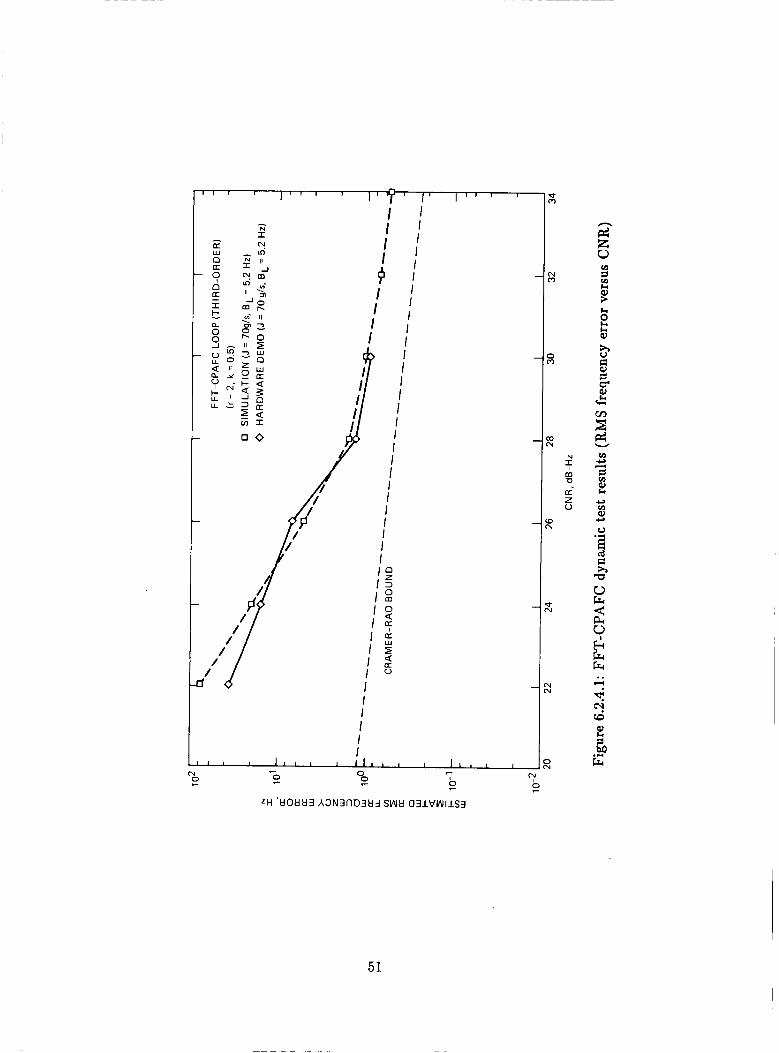
Dynamic tests were carried out using the IEC trajectory, described in Chapter 3. Sample statistics were obtained at various CNRs between 20 and 30 dB-Hz. Results are shown in Figure 6.2.4.1, where good agreement between experiment and theory is apparent.
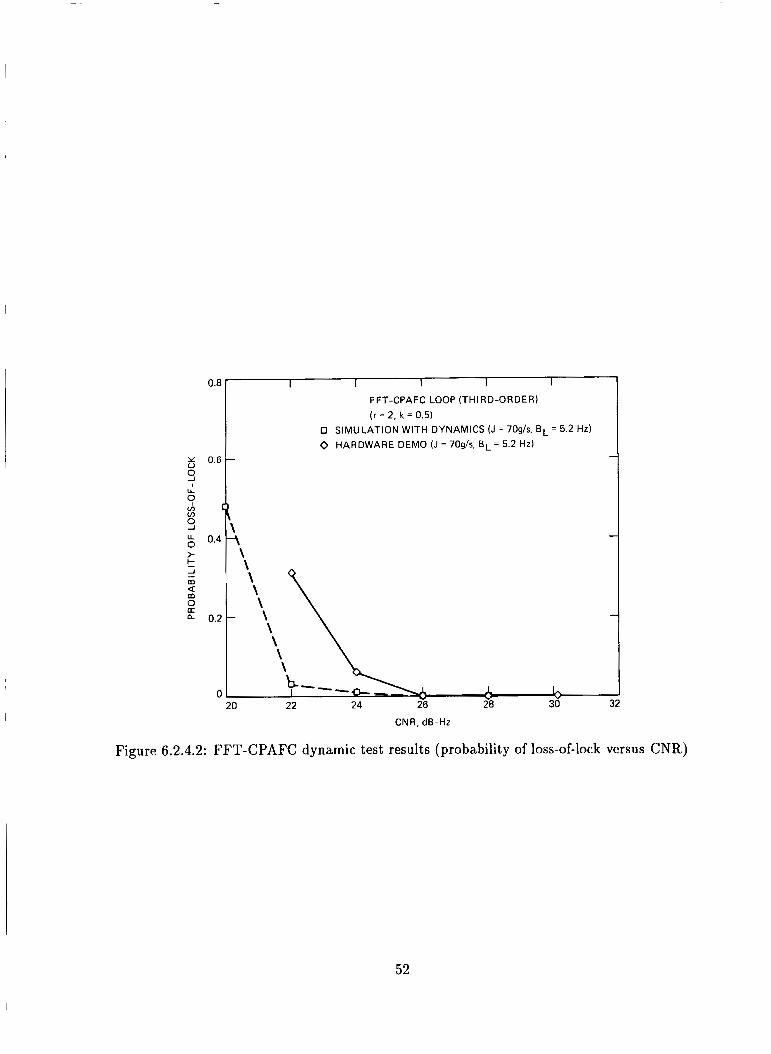
The probability of loss-of-lock was also estimated for the dynamic case. Loss-of-lock occurs when the instantaneous CPAFC error exceeds A250 Hz. Estimated loss-of-lock probabilities are shown in Figure 6.2.4.2, along with the simulated results. The simulation indicates that loss-of-lock becomes a problem near 22 dB-Hz, while for the experiment, this threshold is closer to 24 dB-Hz. This is attributed to amplitude attenuation that is unmodeled in the simulations (see Section 6.3).
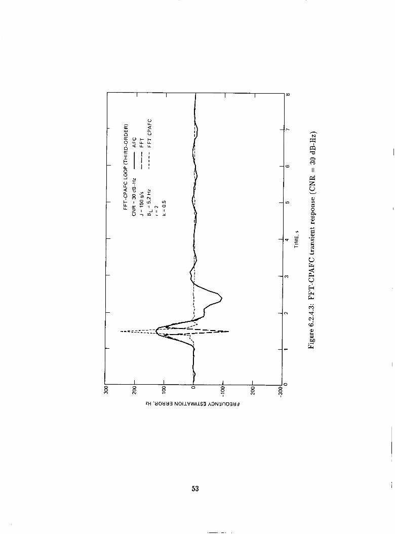
Performance of the third-order CPAFC (and other third-order loops) is very sensitive to loop bandwidth. Since maximum transient error due to jerk is roughly inversely proportional to the third power of the bandwidth, small changes in bandwidth result in large changes in peak error. Since the CPAFC loses lock when the instantaneous frequency error is over 250 Hz, 125 Hz for the FFT, small changes in bandwidth or input dynamics can result in major changes in the performance curves. An example is shown in Figure 6.2.4.3, which is a plot of the instantaneous frequency error of the CPAFC (solid curve) when 150-g/s jerk is applied, along with the FFT estimate (long dashes), and the combined frequency error (short dashes). At roughly 1.5 seconds into the test, the CPAFC error exceeds 125 Hz, which is the upper limit of the FFT estimator. This results in aliasing, whereby the FFT peak suddenly shifts to -125 Hz, yielding an error of roughly 250 Hz in the final estimate. This phenomenon can lead to catastrophic performance degradation, as shown in Figure 6.2.4.4. The situation is easily remedied by increasing the loop bandwidth somewhat (in this case to 7 Hz) in order to reduce the CPAFC’s dynamic excursions.
6.3 Comparison and Discussion I
Performance of the tested algorithms are compared in this section for static and dynamic tests. Performance measures consist of rms frequency error and probability of loss-of-frequency-lock in the presence of dynamics only. Comparisons are made on the basis of measured data, without the application of the calibration curve of Appendix B.
I I
Table 6.1 shows results of rms frequency error comparisons for dynamic tests. Hardware demon- stration and simulation results for the various algorithms are in close agreement, within 5 percent, as shown in this table and in previous figures. The fourth-order EKF performed with the lowest rms frequency error, 3.2 Hz at 26 dB-Hz, but its operating threshold was at 25.8 dB-Hz.
Results for threshold CNR, shown in Table 6.2, exhibit an average 1.4-dB difference between
47
5
4
3
2
1
N I Cc- 2 LT w c t 0 2 5 w 3
LT t U
4
3
2
1
I I I I (a)
I :: I I I I I I I I I I I I I I I I I I I I I
I \ \ I I I I I I I I I I I I I I \ I
EF K (TH I RD-OR DE R ) n = 3 qq = 100 a = 1.06 P L- = 60 dB-Hz
S IMU LAT I ON
NO
I \ \ I \ \
C 2.75 2.95
qq = 100
pc NO
a = 1.06
- = 60 dB-HZ
I ARX MEASUREMENT
3.15 3.35 3.55 3.75
TIME, s
Figure 6.2.3.1: EKF transient response (CNR = 60 dB-Hz): (a) simulation results with 100-g/s jerk; and (b) ARX response to 100-g/s jerk
48
7
E
N I
a' 5 2 a w > V z w 3
a U J
EI
z u 4
3
2 I I
CNR, dB-HZ
23 25 27
Figure 6.2.3.2: EKF dynamic test results (RMS frequency error versus CNR)
49
CNR, dB-HZ
Figure 6.2.3.3: EKF dynamic test results (probability of loss-of-lock versus CNR)
50
I I I
I
51
0.8
0 o.6 t
I I 1 1 I
FFT-CPAFC LOOP (THI RD-ORDER) (r = 2, k = 0.5)
0 SIMULATION WITH DYNAMICS (J = 70g/s, EL = 5.2 HZ) 0 HARDWARE DEMO (J = 7 0 g / ~ , E L = 5.2 HZ)
1
CNR, dB-Hz
Figure 6.2.4.2: FFT-CPAFC dynamic test results (probability of loss-of-lock versus CNR)
52
53

I
I I I I I 4
/ f o a o o
P 7'
4; 1 1
1 1 1 1
I I I I I
I
54
hardware and simulation results, with hardware threshold exceeding simulated (software) values. (Adding calibration data raises the difference to 1.9 dB.) The lowest measured threshold CNR, 23.8 dB-Hz, was achieved by the CPAFC loop, while the highest was in the third-order EKF. The DPLL CNR threshold of 26 dB-Hz is 2.2 dB higher than the CPAFC loop.
The fact that hardware and software agree well in rrns frequency error while showing inferior hardware performance in CNR threshold can be traced to the effect of the amplitude attenuation of input samples due to the digital accumulators that was not modeled in the software simulations. This effect is significant only when the instantaneous frequency error is a large fraction of 250 Hz. To validate this hypothesis we re-tested a third-order CPAFC with a bandwidth of 5.2 Hz, using the 70-g/s trajectory. Figure 6.3.1.a shows the rms frequency error when the amplitude attenuation effect is present and absent, with no significant difference in rms frequency error. Figure 6.3.1.b shows that, for the same configuration, amplitude attenuation degrades CNR threshold by 1-2 dB. This attenuation affects the various algorithms in different ways, depending on the frequency error during the maneuvering. For instance, the DPLL has a 0.8-dB difference between simulated and measured CNR threshold because of its smaller frequency error in the presence of jerk, as shown in Figure 6.2.1.1. Depending on the algorithm in question, it is believed that the effect of amplitude attenuation is 0.8 dB to 1.8 dB in CNR threshold.
Simulated threshold CNRs in Table 6.2 are also slightly different than those of Table 4.1 because of the different trajectories involved. The initial trajectory of Table 4.1 included Doppler rate at the start of the simulations, while the trajectory of Table 6.1 contains a constant initial frequency.
In conclusion, the tested algorithms performed within 0.5 dB of simulations in rms frequency error and within 1.5 dB of simulations in loss-of-lock threshold. The CPAFC loop exibited the lowest threshold and the EKF achieved the smallest rms frequency error.
55
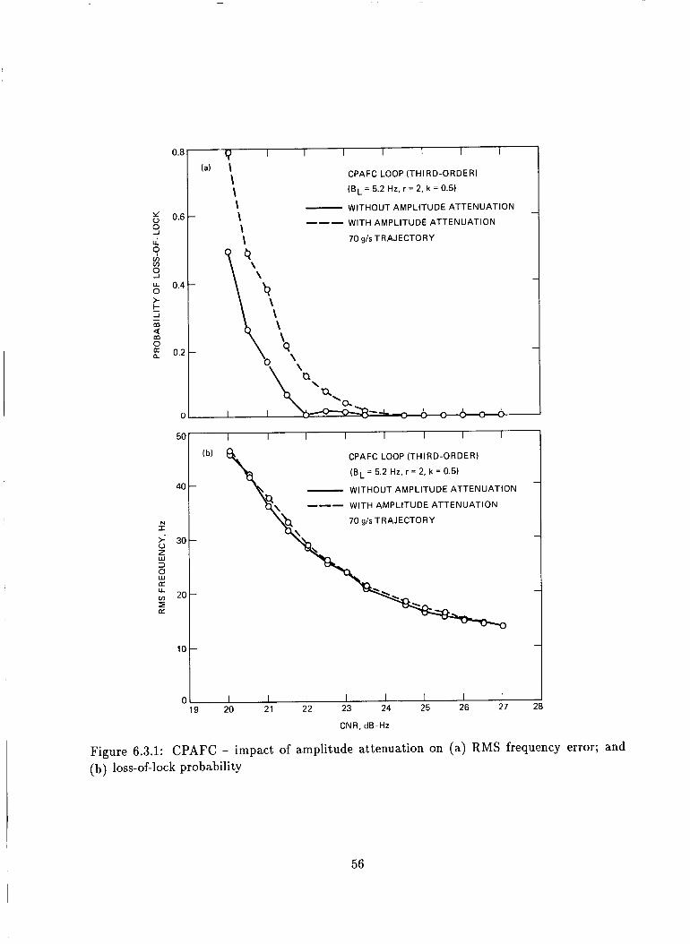
0.8
5 0.6 9 9 I!
U
v) v)
u 0.4 0 > k m
0
-I - 2
0.2
0
50 I I I I I I I I
(b) CPAFC LOOP (THIRD-ORDER)
(BL = 5.2 Hz, r = 2, k = 0.5) - - WITHOUT AMPLITUDE ATTENUATION
--- WITH AMPLITUDE ATTENUATION
40 -
70 g/s TRAJECTORY fl 8 30- -
2 w 3
n t : 2 0 -
z -
10 - -
Q I I I I I I I (a) \
\ \
CPAFC LOOP (THIRD-ORDER)
( B ~ = 5 . 2 H z , r = 2 , k = 0 . 5 )
- WITHOUT AMPLITUDE ATTENUATION
--- WITH AMP L l TU DE ATTENUATION
\ \ \ \ 70 g/s TRAJECTORY
CNR, dB-Hz
Figure 6.3.1: CPAFC - impact of amplitude attenuation on (a) RMS frequency error; and (b) loss-of-lock probability
56
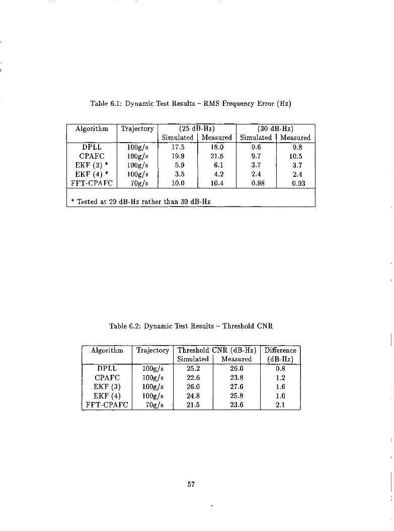
Table 6.1: Dynamic Test Results - RMS Frequency Error (Hz)
Algorithm
DPLL CPAFC
EKF (4) * FFT-CPAFC
EKF (3) *
Trajectory (25 dB-Hz) (30 dB-Hz) Simulated Measured Simulated Measured
lOOg/s 17.5 18.0 9.6 9.8 lOOg/s 19.9 21.6 9.7 10.5
lOOg/s 3.5 4.2 2.4 2.4 lOOg/s 5.9 6.1 3.7 3.7
7Og/s 10.0 10.4 0.98 0.93
* Tested at 29 dB-Hz rather than 30 dB-Hz
Algorithm Trajectory
DPLL lOOg/s
EKF (3) lOOg/s CPAFC lOOg/s
EKF (4) lOOg/s FFT-CPAFC 70g/s
Table 6.2: Dynamic Test Results - Threshold CNR
Threshold CNR (dB-Hz) Difference Simulated Measured (dB-Hz)
25.2 26.0 0.8 22.6 23.8 1.2 26.0 27.6 1.6 24.8 25.8 1 .o 21.5 23.6 2.1
57
Chapter 7
Conclusions
Frequency tracking at low CNRs and in the presence of high dynamics has been the goal of this research effort. Several novel schemes have been introduced, analyzed, and tested in order to validate their performances. These algorithms meet RAJPO’s requirements for operation of the TPS, and offer potential improvements to the existing techniques.
58
Appendix A
Description and Analysis of t h e FFT-CPAFC LOOP
This appendix is devoted to the description, evaluation, and nonlinear analysis of the FFT-CPAFC loop used in the TPS. Simulation results are presented in Section A.l, and the nonlinear perfor- mance analysis is the subject of Section A.2.
A . 1 Simulation Results
The simulation follows the block diagram of Figure 4.7.1, except that 2-ms update rates are used in the CPAFC loop instead of IEC’s multi-rate implementation, and data-wipe is assumed. A type-I11 CPAFC loop was simulated with a single-sided loop bandwidth of 5.2 Hz, and with loop parameters T = 2, k = 0.5. Estimator performance is evaluated using the 100-g/s trajectory described in Section 3.3, and the effects of additive noise are incorporated by adding independent Gaussian noise samples to the signal samples in the I and Q channels. The noise variance is adjusted to yield the desired CNR. Instantaneous frequency estimation errors were recorded at the output of the CPAFC loop (point B in Figure 4.7.1), the output of the FFT error estimator (point C), and the combined estimator output (point D). A characteristic sample sequence of instantaneous estimation errors is shown in Figure A.l.1.a at a CNR of 30 dB-Hz. Note that at this CNR the FFT estimates the CPAFC loop error accurately, yielding a combined rms error of only a few Hertz rms. At lower CNRs, the FFT estimator begins to suffer from outliers, as can be seen in Figure A.l.1.b (CNR = 25 dB-Hz), resulting in degraded performance. At still lower CNR, the CPAFC loop begins to lose lock with high probability. An example of loss-of-lock behavior is shown in Figure A.l.1.c. Loss-of-lock becomes a serious problem below about 22 dB-Hz for this trajectory. At very high CNRs, the dominant error component in the combined estimate is due to dynamics, as shown in Figure A.l.1.d. Therefore, we expect the rms estimation error for the entire trajectory to become independent of CNR for CNRs well above 30 dB-Hz.
The combined frequency estimation error for the entire trajectory was estimated at CNRs ranging
59
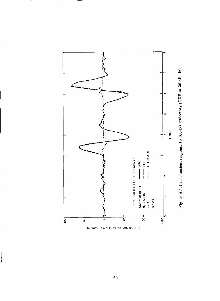
ZH ' t lO t l t l 3 N O I I V W I l S 3 A3N3nD3tld
0 Y
60
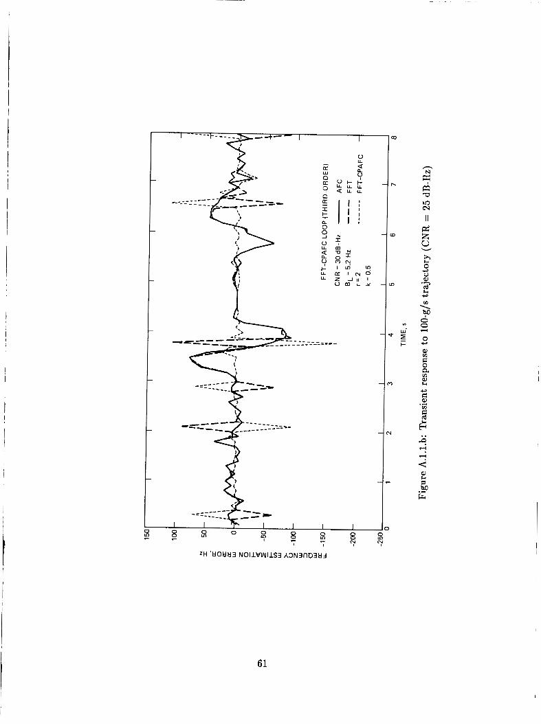
61
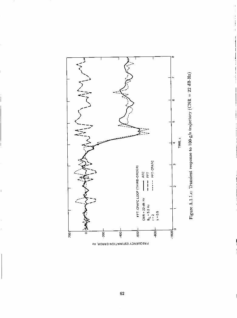
62
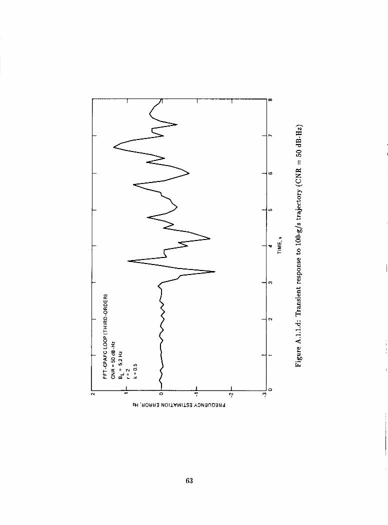
d E
8 I I- 1
9 +
63
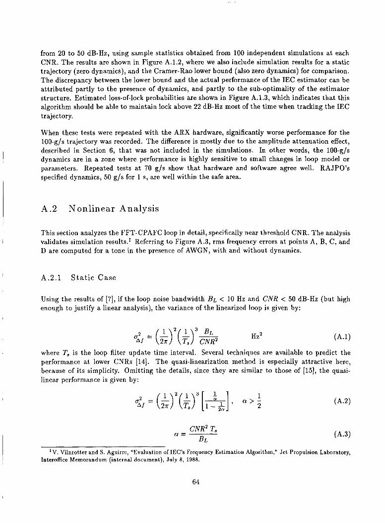
from 20 to 50 dB-Hz, using sample statistics obtained from 100 independent simulations at each CNR. The results are shown in Figure A.1.2, where we also include simulation results for a static trajectory (zero dynamic$), and the Cramer-Rao lower bound (also zero dynamics) for comparison. The discrepancy between the lower bound and the actual performance of the IEC estimator can be attributed partly to the presence of dynamics, and partly to the sub-optimality of the estimator structure. Estimated loss-of-lock probabilities are shown in Figure A.1.3, which indicates that this algorithm should be able to maintain lock above 22 dB-Hz most of the time when tracking the IEC trajectory.
When these tests were repeated with the ARX hardware, significantly worse performance for the lOO-g/s trajectory was recorded. The difference is mostly due to the amplitude attenuation effect, described in Section 6, that was not included in the simulations. In other words, the 100-g/s dynamics are in a zone where performance is highly sensitive to small changes in loop model or parameters. Repeated tests at 70 g/s show that hardware and software agree well. RAJPO’s specified dynamics, 50 g/s for 1 s, are well within the safe area.
A .2 Nonlinear Analysis
This section analyzes the FFT-CPAFC loop in detail, specifically near threshold CNR. The analysis validates simulation results.’ Referring to Figure A.3, rms frequency errors at points A, B, C , and D are computed for a tone in the presence of AWGN, with and without dynamics.
A . 2 . 1 Sta t i c Case
Using the results of [7], if the loop noise bandwidth BL < 10 Hz and CNR < 50 dB-Hz (but high enough to justify a linear analysis), the variance of the linearized loop is given by:
Hz2
where T, is the loop filter update time interval. Several techniques are available to predict the performance at lower CNRs [14]. The quasi-linearization method is especially attractive here, because of its simplicity. Omitting the details, since they are similar to those of [15], the quasi- linear performance is given by:
1 g2, = (&)2(&)3 [-I >
CNR2 T, BL
a =
V. Vilnrotter and S. Aguirre, “Evaluation of IEC’s Frequency Estimation Algorithm,” Jet Propulsion Laboratory, Interoffice Memorandum (internal document), July 8, 1988.
64
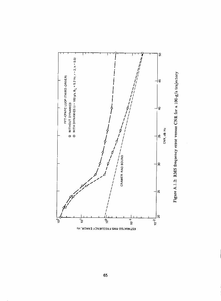
I 1 I I I ' I I I I I ' y ' I I ,
h - I
65
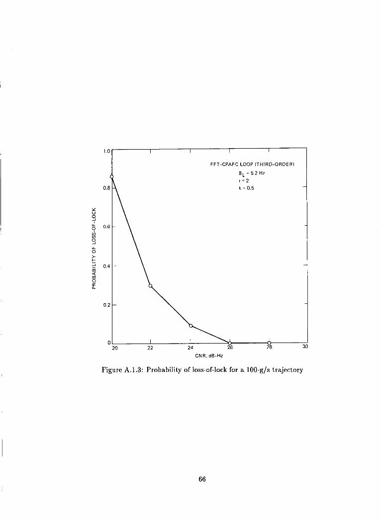
1 .o
I
0.8
Y 0 s 9
s 0.6
VI v)
L L
0 t k 2 0.4 m
0 n n
2
0.2
0
FFT-CPAFC LOOP (THIRD-ORDER)
BL = 5.2 HZ r = 2 k = 0.5
CNR. dB-HZ
Figure A.1.3: Probability of loss-of-lock for a 100-g/s trajectory
66
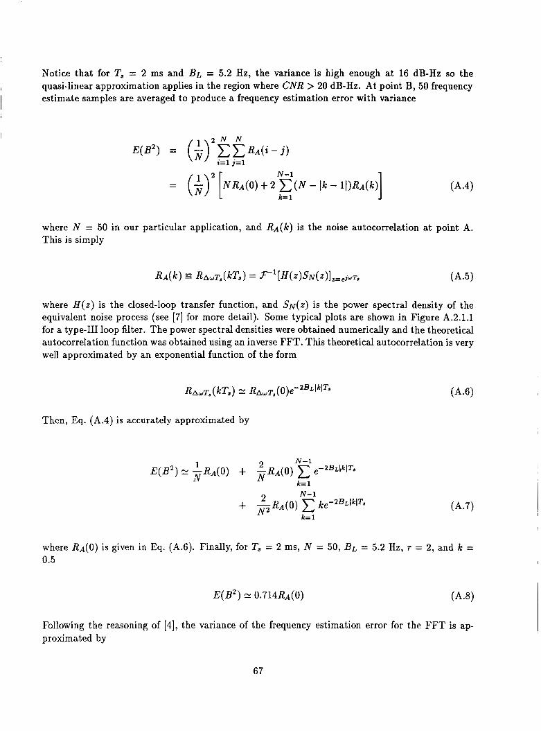
Notice that for T, = 2 ms and BL = 5.2 Hz, the variance is high enough at 16 dB-Hz so the I quasi-linear approximation applies in the region where CNR > 20 dB-Hz. At point B, 50 frequency
estimate samples are averaged to produce a frequency estimation error with variance I
where N = 50 in our particular application, and &(k) is the noise autocorrelation at point A. This is simply
where H ( z ) is the closed-loop transfer function, and S N ( Z ) is the power spectral density of the equivalent noise process (see [7] for more detail). Some typical plots are shown in Figure A.2.1.1 for a type-I11 loop filter. The power spectral densities were obtained numerically and the theoretical autocorrelation function was obtained using an inverse FFT. This theoretical autocorrelation is very well approximated by an exponential function of the form
Then, Eq. (A.4) is accurately approximated by
where RA(O) is given in Eq. (A.6). Finally, for T, = 2 ms, N = 50, BL = 5.2 Hz, T = 2, and k = 0.5
Following the reasoning of [4], the variance of the frequency estimation error for the FFT is ap- proximated by
67
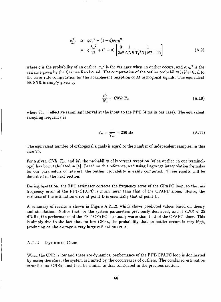
2 a,, N
where q is the probability of an outlier, au2 is the variance when an outlier occurs, and U C R ~ is the variance given by the Cramer-Rao bound. The computation of the outlier probability is identical to the error rate computation for the noncoherent reception of M orthogonal signals. The equivalent bit SNR is simply given by
(A.lO)
where T,, = effective sampling interval at the input to the EFT (4 ms in our case). The equivalent sampling frequency is
( A . l l )
The equivalent number of orthogonal signals is equal to the number of independent samples, in this case 25.
For a given CNR, T,,, and M, the probability of incorrent reception (of an outlier, in our terminol- ogy) has been tabulated in [4]. Based on this reference, and using Lagrange interpolation formulas for our parameters of interest, the outlier probability is easily computed. These results will be described in the next section.
During operation, the FFT estimator corrects the frequency error of the CPAFC loop, so the rms frequency error of the FFT-CPAFC is much lower than that of the CPAFC alone. Hence, the variance of the estimation error at point D is essentially that of point C.
A summary of results is shown in Figure A.2.1.2, which shows predicted values based on theory and simulation. Notice that for the system parameters previously described, and if CNR < 25 dB-Hz, the performance of the FFT-CPAFC is actually worse than that of the CPAFC alone. This is simply due to the fact that for low CNRs, the probability that an outlier occurs is very high, producing on the average a very large estimation error.
A.2.2 Dynamic Case
When the CNR is low and there are dynamics, performance of the FFT-CPAFC loop is dominated by noise; therefore, the system is limited by the occurrences of outliers. The combined estimation error for low CNRs must then be similar to that considered in the previous section.
68
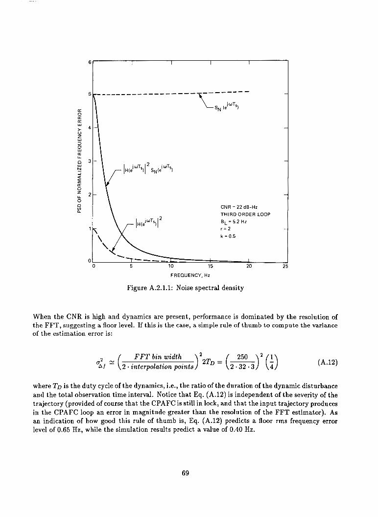
E
5
a 2 > 4
El
a W
0 z W 3
a
0 3 2 Q E a 0
0
n
LL
W
J
t 2
2
1
0
I THIRD ORDER LOOP BL = 5.2 HZ r = 2
\ A k = 0.5
I 1 5 10 15 20
FREQUENCY, Hz
Figure A.2.1.1: Noise spectral density
When the CNR is high and dynamics are present, performance is dominated by the resolution of the FFT, suggesting a floor level. If this is the case, a simple rule of thumb to compute the variance of the estimation error is:
u2 21 ( FFT bin width ) 2 2 T ~ = ( 250 )'(a) Af 2 interpolation points 2 . 3 2 - 3
(A.12)
where TD is the duty cycle of the dynamics, i.e., the ratio of the duration of the dynamic disturbance and the total observation time interval. Notice that Eq. (A.12) is independent of the severity of the trajectory (provided of course that the CPAFC is still in lock, and that the input trajectory produces in the CPAFC loop an error in magnitude greater than the resolution of the FFT estimator). As an indication of how good this rule of thumb is, Eq. (A.12) predicts a floor rms frequency error level of 0.65 Hz, while the simulation results predict a value of 0.40 Hz.
69
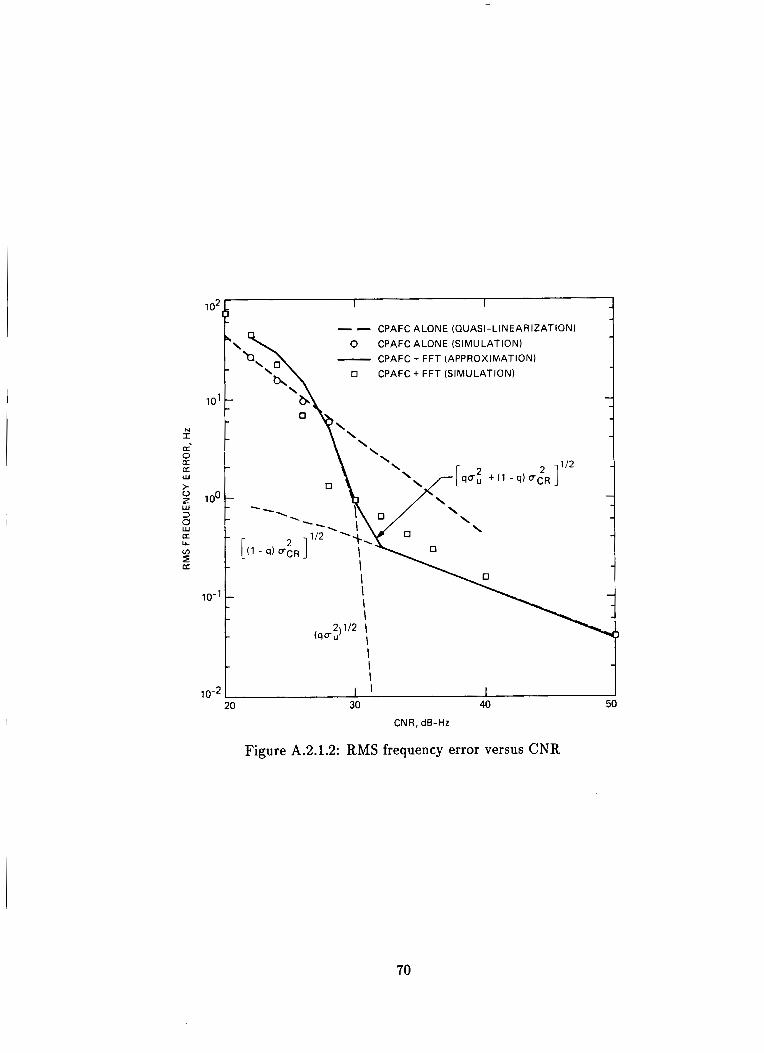
Figure A.2.1.2: RMS frequency error versus CNR
70
Appendix B
C alib r at ion Measurements
In order to make meaningful comparisons between theoretical, experimental, and simulated perfor- mance, accurate calibration of the test equipment is essential. Specifically, the CNR presented to each algorithm must be known. Although the CNR at the output of the signal generator assembly (SGA) is beleived to be known to within 0.1 dB, the various losses due to cabling, attenuation, mixing, filtering, and A/D conversion are not well understood. Thus, the CNR of the sampled sequence presented to the algorithms may differ markedly from the nominal settings on the SGA. Therefore, we seek to develop a procedure for determining the CNR of the digital sequence directly from the complex samples generated by the A/D converter. Our approach will be to estimate the signal amplitude and noise variance first, and subsequently obtain a CNR estimate from these quantities.
B .1 Mathematical M ode1
When operating in the PLL configuration, the GPS testbed can be modeled as in Figure B.l.l. The in-phase samples xi and quadrature samples yj can be represented as
2; = A COS(+^) -+ nzi (B.la)
yj = A sin($;) i- nyi (B.lb)
where $i is the phase error, A the signal amplitude, and n,, and nyi are independent zero mean Gaussian random variables with variance a2 = N0/2TS. Since the in-phase samples are proportional t o A for small $j, it is convenient to use them for estimating A and No, while adjusting the loop bandwidth to effectively eliminate the effects of the phase error 4;. In this way, sample statistics can be used to estimate the signal amplitude and noise variance to virtually any desired accuracy.
71
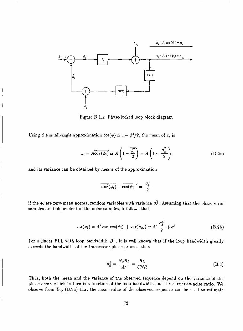
Jli
Figure B. 1.1: P hase-locked loop block diagram
Using the small-angle approximation cos(q5) N 1 - cj2/2, the mean of 5; is
- 2; = A c o s ( ~ ; ) 21
and its variance can be obtained by means of the approximation
(B.2a)
if the 4; are zero-mean normal random variables with variance u$. Assuming that the phase error samples are independent of the noise samples, it follows that
2 4 2 var(2;) = A2var [cos(&)] -t var(n,,) A - + Q 2 (B.2b)
For a linear PLL with loop bandwidth BL, it is well known that if the loop bandwidth greatly exceeds the bandwidth of the transceiver phase process, then
Thus, both the mean and the variance of the observed sequence depend on the variance of the phase error, which in turn is a function of the loop bandwidth and the carrier-to-noise ratio. We observe from Eq. (B.2a) that the mean value of the observed sequence can be used to estimate
72
the signal amplitude directly, provided the phase-error variance is reduced to an acceptable level. In principle, this can be achieved at any CNR by making the loop bandwidth sufficiently small. Suppose we wish to limit the bias term u24/2 to a value no greater than 6. Then for any CNR, the loop bandwidth that achieves this limit is
For example, at CNR = 30 dB-Hz, BL 5 2 Hz guarantees that 6 5 O . l % , while at CNR = 20 dB-Hz, BL 5 0.2 Hz guarantees the same percentage bias. As long as this bias is substantially smaller than the rms estimation error, its effect on the amplitude estimate can be ignored.
The expression for the variance of the observables in Eq. (B.2b) can also be simplified when operat- ing with narrow bandwidths at high CNRs. Using Eq. (B.3) in Eq. (B.2b), and defining B, = l/Ts, it follows that
for BL << B, and BL/CNR < 1. As long as the above conditions are satisfied, we can use the approximations
5i 2i A (B.6a)
var(x;) 2i u2 (B.6b)
These approximations help to simplify the determination of estimator performance, and will be assumed in the following analysis.
B .2 Estimator S t ruc ture
The following estimator was chosen for determining CNR from the in-phase samples: the sample mean is used to estimate the signal amplitude A, while the sample variance is used to determine NO. The ratio of the mean-value squared to noise spectral level is used to estimate CNR. Thus we have
. N (B.7a)
73
(B.7b)
(B.7c)
If the loop bandwidth has been selected to effectively eliminate the bias term, the variance of the resulting estimates may be obtained by assuming that the rms estimation errors for both the signal amplitude and the noise spectral level are small compared to the estimates. Then we can write
A ^ = A + E A (B.8a)
(B.8c)
where EA and C N ~ are taken to be zero-mean random variables. The variance of the resulting estimation error may be bounded by means of the sample statistics, but care must be taken to account for correlations in the error terms. These correlations arise because the sample variance formula makes use of the sample mean. With the help of the inequality ( E A E N ~ I 5 ffAaNo we can bound the variance of the CNR estimate as
In order to obtain numerical answers, the components of the bound must be determined. First consider the variance of the amplitude estimate, A . Using the model of Eq. (B.6), it follows that the variance of the sample mean is
(B.lO) u2 02 = var(EA) N -
A N
The variance of the sample variance involves the fourth central moment, p4, of the population distribution. Since for zero-mean normal random variables p4 = 3a4, it follows that
4Ts2 N - 3 8TS2 a4 3a - (-)a41 - N - - [ N N - 1 u 5 3 var(ENo) = No
(B. l l )
74
for the case N >> 3. Direct substitution into Eq. (B.9) yields
(B.12)
Referring to Eq. (B.8c), we note that the ratio C 'NR/CNR = 1 + 6, where 6 is a zero-mean random variable whose variance is bounded by the right-hand-side of Eq. (B.12). Denoting the upper bound on the standard deviation of this random variable as o,", we can approximately bound C 'NR/CNR in the interval (1 - oe", 1 + o ~ " ) . Since ueu is itself a function of CNR, the width of these intervals varies as shown in Figure B.2.1, where the upper and lower envelopes are expressed in dB to facilitate comparison with the numerical results that follow.
I
B .3 Numerical Results
Numerical calibration results were obtained using the ARX in the PLL configuration. A loop bandwidth of BL = 0.1 Hz was selected to ensure that the bias term remains less than 0.1 percent in the range of interest (20 5 CNR 5 30 dB-Hz). Since the resulting bias in the CNR estimates is insignificant compared to the roughly 0.2-dB estimation error envelope, the effects of bias on the CNR estimates can indeed be ignored.
The calibration curve of Figure B.3.1 was obtained by processing N = 4000 in-phase samples in the manner described above, at 1-dB intervals in the range 20 5 CNR 5 30 dB-Hz. This particular value of N was chosen because it yielded adequate performance, and because the framework already existed for recording 4000 in-phase and quadrature samples (there are exactly 4000 samples in the 8-s common trajectory used for evaluating the algorithms). Note that the spread of the data- points around the best-fit line is consistent with the error envelopes shown in Figure B.3.1. It can be concluded from the correction curve that a positive correction should be applied at all CNRs within the range of interest, from roughly 0.1 dB at 30 dB-Hz to nearly 0.8 dB at 20 dB-Hz. The reason for this miscalibration is not well understood at this time.
75
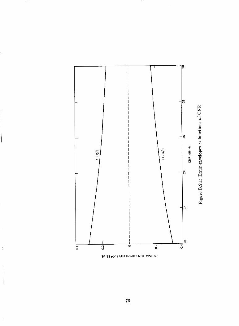
BP 'S3d013AN3 t lOt l t l3 NOIIVVUIlS3
I
I
I
N
F m
a* 0
2 0
r
v v
3
76
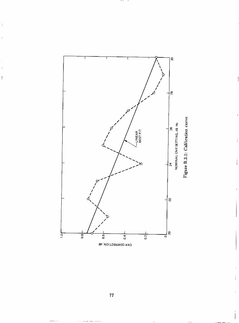
BP 'N01133klkl03 k l N 3
0 m
P N
0
b v
rl rl
> J
77
Appendix C
A R X Software Modifications
This appendix describes the modifications to the ARX software that were implemented in order to test the various algorithms.
In ADRCF, the subcarrier and symbol synchronization loop filters have been removed. A trajectory was added to the NCOl command (see Figure 5.2.1.1). The trajectory insertion is requested by the operator. The operator also requests the specific algorithm for generating the NC02 command. The NC02 command is the frequency estimate from the algorithm chosen. These added algorithms are the DPLL, which is the same as that used in the carrier loop of the ARX, the CPAFC loop, the EKF, and the FFT-CPAFC. The ARX data acquisition was totally replaced by the GPS data acquisition. For the purpose of analysis, the ARX acquires I, Q, power, and SNR samples for different sampling intervals. These samples are continuously acquired during tracking. A tracking period can be any length of time. The ARX attempts to compute statistics and display them in real time. When the ARX computations fail to keep up with the sampling, sample acquisition is halted temporarily and the sample loss is noted.
For the purpose of analysis, the data that the GPS acquires depend on the algorithm that has been chosen by the operator. The choice of the DPLL and CPAFC algorithms will cause acquisition of I, Q, NCOl command, NC02 command, the output of the cross-product, and the output of the cross-product integrator. The choice of the EKF algorithm will cause acquisition of I, Q, the NC02 command, and the state vector of the Kalman filter. The choice of the FFT-CPAFC algorithm will cause acquisition of the NCOl command and the NC02 command. The GPS sampling interval is fixed at 2 ms and the period of acquisition during the track is 8 s. By assigning a 4000-element buffer (500 samples per second times eight seconds) for each test, no samples are lost.
The acquisition of I and Q samples for performing the FFTs was also modified. The ARX needs the I and Q samples to compute FFT for preacquisition, which does not have the time constraint imposed by the GPS. It does, however, require that the number of FFTs performed be open ended so that this number can be chosen by the operator; the system always performs 80 FFTs for each test run. The ARX toggles between two buffers, each with the length needed to compute one FFT. It waits until a buffer has been freed by the program that performs the FFT before refilling that buffer. The GPS has 80 buffers assigned, and the last sample of any buffer is contiguous with the
78
first sample of the next buffer. The operator defines the FFT size in both systems. Additionally, the GPS allows the operator t o set the number of data points to be transformed.
~ In ARPRINT, the monitor display sections and the logging sections associated with the subcarrier and symbol synchronization loops were excised. Added to the monitor display were frequency estimation errors from the FFT and the EKF algorithm, and indicators showing which algorithm is currently in effect. Logic was added to control program flow associated with FFT requests and program flow associated with multiple test runs. A test run is one 8-s track. The GPS has five sections for data reduction and disk logging, as described below.
Section 1 is for the FFT-CPAFC loop. It has two subsections depending on whether the operator has requested all 80 estimates of each test run or statistics. The statistics are the rms and mean frequency errors and lock condition for each test run and the average rms, mean, and probability of loss-of-lock for multiple test runs. The number of test runs are requested by the operator. The remaining sections are for all other algorithms. Section 2 handles the case with no dynamics. It generates 4000 entries of raw data and does not do multiple test runs. Section 3 handles the caseJ with no dynamics. It computes statistics and can perform multiple test runs. Section 4 handles the case with dynamics and generates 4000 entries of raw data. It does not do multiple test runs. Section 5 handles the case with dynamics. It computes statistics and can do multiple test runs. In Sections 2, 3 , 4 , and 5 there are some differences in the data reduction and disk logging capability depending on the algorithm in effect.
Section 1, the output of the FFT-CPAFC algorithm, comprises 5 columns of 80 entries per column. Column 1 is the sample number (number 1 to 80). Column 2 is the average of 50 samples of the command to NC02. Column 3 is the estimate from the FFT. Column 4 is the difference between Columns 2 and 3. Column 5 is the sum of Columns 4 and the average of 50 commands to NCO1. The statistics are performed on the command to NC02 plus the command to NCOl minus the estimate from the FFT.
Section 2 produces one output for the EKF algorithm and another for the CPAFC and DPLL algorithms. Both outputs have 4000 entries. The EKF algorithm has 7 columns and the CPAFC and DPLL algorithms have 6 columns. For the EKF algorithm, Column 1 is the sample number k for k = 1, . . ., 4000, Column 2 is p(k), Column 3 is z t ( k ) , Column 4 is z ~ ( k ) , Column 5 is ~ ( k ) , Column 6 is q(k) and Column 7 is g(k). For the CPAFC and DPLL algorithms, Column 1 is the sample number, Column 2 is the discriminator output, Column 3 is the integrator output (Columns 2 and 3 are zero for the PLL algorithm), Column 4 is the command to NC02, Column 5 is I, and Column 6 is Q .
Section 3 produces 3 columns of 4000 entries. Column 1 is the sample number, Column 2 is the command to NCO1, and Column 3 is the command to NC02. If the EKF algorithm is in effect, Column 2 is the average of two consecutive commands to NCO1.
Section 4 computes and produces the statistics on both frequency estimate (the command to NC02) and phase estimate (Q).
Section 5 computes and produces statistics on the error in frequency estimation. This error is the difference between the command to NCOl and the command to NC02. If the EKF algorithm is
79
in effect, the average of two consecutive NCOl commands is used to compute the difference. If the difference exceeds 250 Hz or is less than -250 Hz, an out-of-lock condition is recorded.
In ARFAST, the averaging of FFTs that the ARX requires was removed. The 200-ms delay for each AP-4 access was also removed. The ARX requires a greater update rate from the A/D convertors than the GPS and thereby needs to reduce traffic on the multibus. The GPS requires a greater speed in computing FFTs. Several AP-4 commands were added so that the GPS can do a vector multiplication. Buffer handling was changed to conform with the changes in ADRCF. Logic was added to accumulate 80 FFT estimates. The power spectrum, peak search, and quadratic interpolation to improve the estimates are the same in both systems.
In ARPCALC, the changes were minimal. The calculations associated with the subcarrier and symbol synchronization loops were simply ignored rather than removed. One gain was added for use in the EKF algorithm.
In ARINITL, the initializing of the parameters used by excised portions of the software were ignored rather than removed. The parameters used by the real-time software are initialized and the trajec- tory generated. The parameter values that ARINITL reads from a disk file, upon operator request, were modified to reflect the added parameters of the GPS system (compatible with ARPENTR).
In ARPENTR, the ARX portions associated with the subcarrier and symbol synchronization loops were excised. A section was added to accept operator inputs for algorithm selection. Should the operator select the FFT-CPAFC algorithm, ARPENTR asks the operator to request the number of I and Q samples, and the FFT size. Should the operator select the EKF algorithm, ARPENTR asks the operator to input the Kalman filter steady-state gains. The parameter values that ARPENTR writes to a disk file, upon operator request, were modified to reflect the added parameters of the GPS system (compatible with ARINITL).
In ARMENUS, the statements associated with the subcarrier and symbol synchronization loops were excised and the statement concerning preacquisition was removed. Statements were added to accommodate algorithm selection.
In ARGLOBS, the global variables not applicable to the GPS were ignored rather than removed. All newly defined global variables were added.
80
Appendix D
Glossary
S
ms Hz
m m/s
g AFC ALS ARX BPSK CPAFC CNR CRT DFT DPLL DSN EKF FEKF FFT GPS IEC JPL MLE NASA NCO ODAFC PLL RAJPO RMS
- second - millisecond - Hertz - meter per second - meter - gravity acceleration factor - Automatic Frequency Control (loop) - Adaptive Least Squares - (NASA’s) Advanced Receiver - Bi-Phase Shift Keying - Cross-Product Automatic Frequency Control (loop) - Carrier (power) to Noise Ratio - Cathode Ray Tube (terminal) - Discrete Fourier Transform - Digital PLL - (NASA’s) Deep Space Network - Extended Kalman Filter - Frequency Extended Kalman Filter - Fast Fourier Transform - Global Positioning System - Interstate Electronics Co. - Jet Propulsion Laboratory - Maximum Likelihood Estimator - National Aeronautics and Space Administration - Numerically Controlled Oscillator - Overlapping DFT-based AFC - Phase-Locked Loop - (GPS) Range Applications Joint Program Office - Root Mean Square
81
SGA I TPS
TTFF VLSI
- Signal Generator Assembly - Translator-Transdigitizer Processing System - Time To First Fix - Very Large Scale Integration
82
Appendix E
References
1. “System Specification For Global Positioning System (GPS) Based Translator Processing System (TPS), Type A,” RAJPO Specification 7383826, USAF AD/YI, Eglin AFB, FL, March 31, 1987.
2. W. Hurd, J. Statman, and V. Vilnrotter, High Dynamic GPS Receiver Validation Demon- stmtion Final Report, JPL Publication 85-74, Jet Propulsion Laboratory, Pasadena, CA, September 1985.
3. Contract NAS7-918, Task Order RE-182, Amendment 452A, “High Dynamics GPS Range Instrumentation Receiver,” Jet Propulsion Laboratory, November 1985.
4. W. Hurd, J. Statman, and V. Vilnrotter, “High Dynamic GPS Receiver Using Maximum Likelihood Estimation and Frequency Tracking,” IEEE Zhnsactions on A ES, AES-23, No. 4, July 1987.
5. V. A. Vilnrotter, S. Hinedi, and R. Kumar, A Comparison o f h q u e n c y Estimation Techniques for High Dynamic Zhjectories, JPL Publication 88-21, Jet Propulsion Laboratory, Pasadena, CA, September 15, 1988.
6. B. D. 0. Andersen and J. B. Moore, Optimal Filten’ng, Prentice Hall, Englewood Cliffs, NJ, 1979.
7. S. Aguirre, “An Automatic Frequency Control Loop Using Overlapping DFTs,” TDA Progress Report 42-94, pp. 222-231, Jet Propulsion Laboratory, Pasadena, CA, June 15, 1988.
8. S. Hinedi, “An Extended Kalman Filter Based Automatic Frequency Control Loop,” TDA Progwss Report 42-95, pp. 219-228, Jet Propulsion Laboratory, Pasadena, CA, November 15, 1988.
9. R. Kumar, “Fast Frequency Estimation via Adaptive Least Squares Algorithm,” TDA Progress Report 42-85, pp. 53-61, Jet Propulsion Laboratory, Pasadena, CA, May 15, 1986.
10. R. Kumar, “Differential Sampling for Fast Frequency Acquisition via Adaptive Extended Least Squares Algorithm,” Proceedings of the International Telemetering Conference, San Diego, pp. 191-201, October 1987.
83
11. U. Cheng, “Performance of a Class of Parallel Spread Spectrum Code Acquisition Schemes in the Presence of Data Modulation,” IEEE Zhnsactions on Communications, Volume 36, No. 5, pp. 596-604, May 1988.
12. U. Cheng, W. Hurd, and J. Statmam, “Spread Spectrum Code Acquisition in the Presence of Doppler Shift and Data Modulation,” accepted for publication in the IEEE Zhnsactions on Communications.
13. D. H. Brown and W. J. Hurd, “DSN Advanced Receiver: Breadboard Description and Test Results,” TDA Pmgess Report 42-89, pp. 48-66, Jet Propulsion Laboratory, Pasadena, CA, May 15, 1987.
14. W. C. Lindsey, Synchmnization Systems in Communication and Control, Prentice Hall, En- glewood Cliffs, NJ, 1972.
15. J. A. Develet, “A Threshold Criterion for Phase-Lock Demodulation,” IRE Pmedings , Vol. 51, No. 2, pp. 349-356, February 1963.
16. W. C. Lindsey and M. Simon, Telecommunication Systems Engineering, Prentice Hall, En- glewood Cliffs, N J , 1973.
84
TECHNICAL REPORT STANDARD TITLE PAGE
1. Report No. 88-35 2. Government Accession No.
High-Dynamic GPS Tracking (Final Report)
17. Key Words (Selected by Author($)) GPS, high dynamic tracking, low C N R , P P L , E K F , FFT, CPAFC
7. Author(s) Hinedi, S . and Statman, J .
18. Distribution Statement
Unclassified -- Unlimited
~ ~~ ~~ ~
9. Performing Organization Name and Address JET PROPULSION LABORATORY California Institute of Technology 4800 Oak Grove Drive Pasadena, California 91109
19. Security Classif. (of this report)
Unc 1 ass i f i ed
12. Sponsoring Agency Name and Address
NATIONAL AERONAUTICS AND SPACE ADMINISTRATION Washington, D.C. 20546
20. Security Clarsif. (of this page) 21. No. of Pages 22. Price
Uncl a s s i f i ed 93
3. Recipient's Catalog No.
5. Report Date
6. Performing Organization Code December 15, 1988
8. Performing Organization Report No,
IO. Work Unit No.
1 1 . Contract or Grant No.
13. Type of Report and Period Covered NAS7-9 18
14. Sponsoring Agency Code
15. Supplementary Notes
16. Abstract This report presents the r e su l t s of comparing four d i f f e ren t frequency timation schemes in the presence of high dynamics and low carr ier- to-noise r a t io s .
The comparison i s based on measured data from a hardware demonstration. The tes ted algorithms include a d i g i t a l phase-locked loop, a cross-product automatic frequency tracking loop, and extended Kalman f i l t e r , and f i n a l l y , an FFT-aided cross-product frequency tracking loop. error performance and t h e i r a b i l i t y t o maintain lock during severe maneuvers a t various carr ier- to-noise r a t i o s .
The tracking algorithms a r e compared on t h e i r frequency
The measured results a r e shown t o agree with simulation r e su l t s car r ied o u t and reported previously.