Genome Rearrangement PhylogenyGenome Rearrangement Phylogeny
Robert K. JansenSchool of Biology
University of Texas at Austin
Bernard M.E. MoretDepartment of Computer Science
University of New Mexico
Li-San Wang Tandy WarnowDepartment of Computer Sciences
University of Texas at Austin

2
Outline
• Introduction• Genome rearrangement phylogeny
reconstruction• Application• Other methods• Future research
3
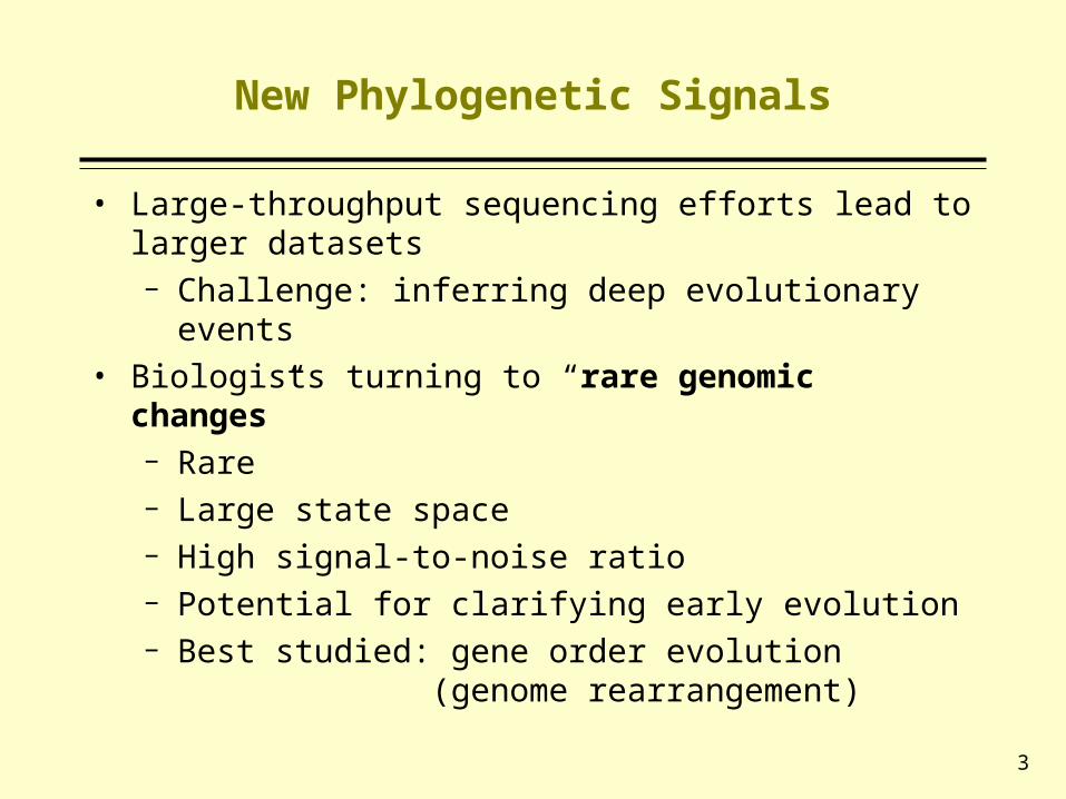
New Phylogenetic Signals
• Large-throughput sequencing efforts lead to larger datasets− Challenge: inferring deep evolutionary events
• Biologists turning to “rare genomic changes”− Rare− Large state space− High signal-to-noise ratio− Potential for clarifying early evolution− Best studied: gene order evolution
(genome rearrangement)

4
Genomes As Signed Permutations
1 –5 3 4 -2 -6 or5 –1 6 2 -4 -3 etc.
5
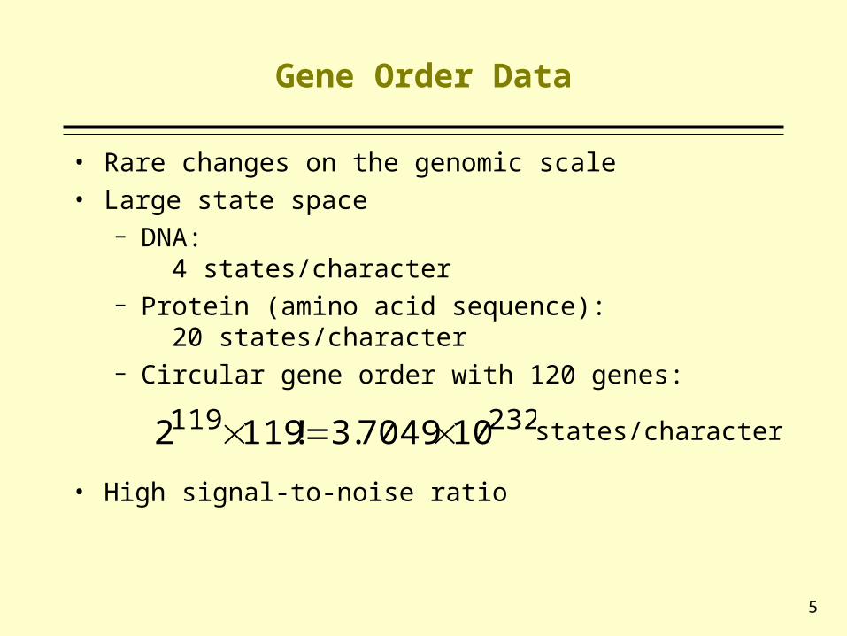
Gene Order Data
• Rare changes on the genomic scale• Large state space
− DNA: 4 states/character
− Protein (amino acid sequence): 20 states/character
− Circular gene order with 120 genes:
• High signal-to-noise ratio
232119 107049.3!1192 states/character
6
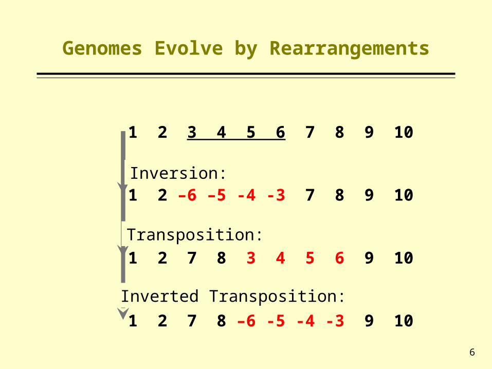
Genomes Evolve by Rearrangements
1 2 3 4 5 6 7 8 9 10
1 2 –6 –5 -4 -3 7 8 9 10
1 2 7 8 3 4 5 6 9 10
1 2 7 8 –6 -5 -4 -3 9 10
Inversion:
Transposition:
Inverted Transposition:

7
Edit Distances Between Genomes
• (INV) Inversion distance [Hannenhalli & Pevzner 1995]
− Computable in linear time [Moret et al 2001]• (BP) Breakpoint distance [Watterson et al. 1982]
− Computable in linear time− NJ(BP): [Blanchette, Kunisawa, Sankoff, 1999]
1 2 3 4 5 6 7 8 9 10
1 2 3 -8 -7 -6 4 5 9 10
A =
B =
BP(A,B)=3

8
Our Model: the Generalized Nadeau-Taylor Model [STOC’01]
• Three types of events: − Inversions (INV)− Transpositions (TRP)− Inverted Transpositions (ITP)
• Events of the same type are equiprobable• Probabilities of the three types have fixed ratio
• We focus on signed circular genomes in this talk.
9
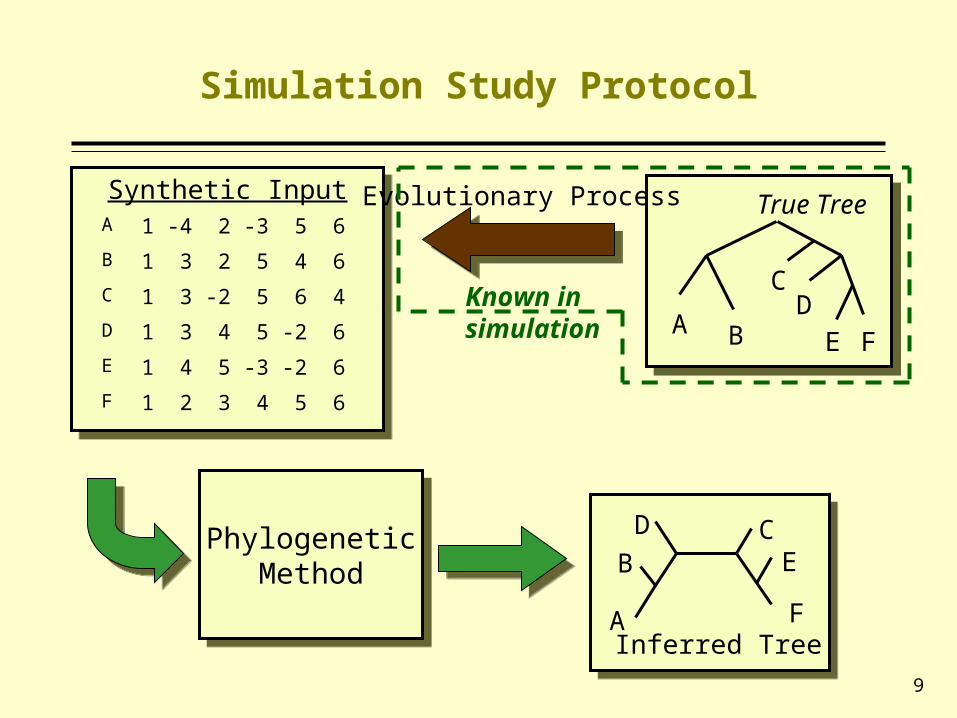
Simulation Study Protocol
Synthetic InputSynthetic Input
PhylogeneticMethod
PhylogeneticMethod
DB
A
CE
FInferred Tree
A B
CD
E F
True TreeEvolutionary Process
Known in simulation
A 1 -4 2 -3 5 6
B 1 3 2 5 4 6
C 1 3 -2 5 6 4
D 1 3 4 5 -2 6
E 1 4 5 -3 -2 6
F 1 2 3 4 5 6

10
Quantifying Error
FN: false negative (missing edge)
1/3=33.3% error rate
A B
CD
E F
True Tree
A B
CD
E F
True Tree
A B
CD
E F
True Tree DB
A
CE
F
Inferred Tree
DB
A
CE
F
DB
A
CE
F
Inferred Tree

11
Outline
• Genome rearrangement evolution• Genome rearrangement phylogeny
reconstruction• Application• Other methods• Future research

12
Gene Order Parsimony
Length (T) = min AX+BX+XY+CY+YZ+DZ+YW+EW+FW
X,Y,Z,W
A
B
C
D
E
F
X
Y
Z W
A
B
C
D
E
F
X
Y
Z W
A
B
C
D
E
F

13
Breakpoint Phylogeny[Sankoff & Blanchette 1998]
• “Maximum Parsimony”-style problem:− Find tree(s), leaf-labeled by genomes, with
shortest breakpoint length
• NP-hard problem on two levels:− Find the shortest tree (the space of trees has
exponential size)− Given a tree, find its breakpoint length
(Even for a tree with 3 leaves, but can be reduced to TSP)
• BPAnalysis [Sankoff & Blanchette 1998] − Takes 200 years to compute our 13-taxon
dataset on a Sun workstation

14
X
Y
Z W
A
B
C
D
E
F
X
Y
Z W
A
B
C
D
E
F
BPAnalysis
• Tree length evaluation for EVERY tree• Given a fixed tree topology, evaluate the tree
length:− Iteratively evaluate the median problem (tree
length for a 3-leaf tree)
A
BY
X’C
Z
Y’X’
15
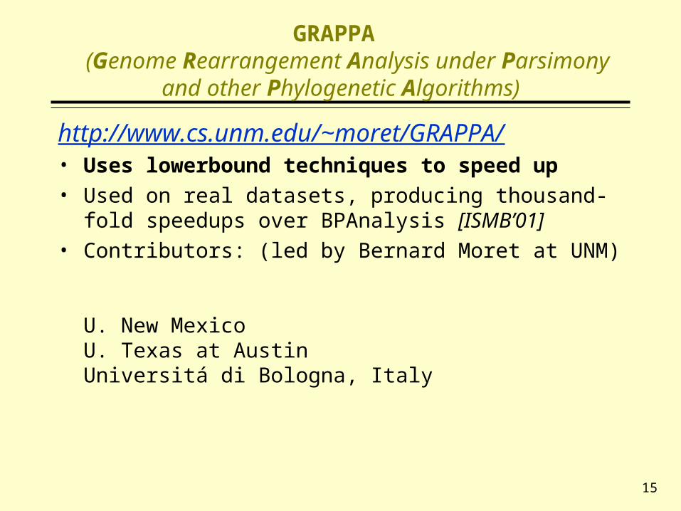
GRAPPA (Genome Rearrangement Analysis under
Parsimony and other Phylogenetic Algorithms)
http://www.cs.unm.edu/~moret/GRAPPA/• Uses lowerbound techniques to speed up• Used on real datasets, producing thousand-fold
speedups over BPAnalysis [ISMB’01]• Contributors: (led by Bernard Moret at UNM)
U. New MexicoU. Texas at AustinUniversitá di Bologna, Italy
16
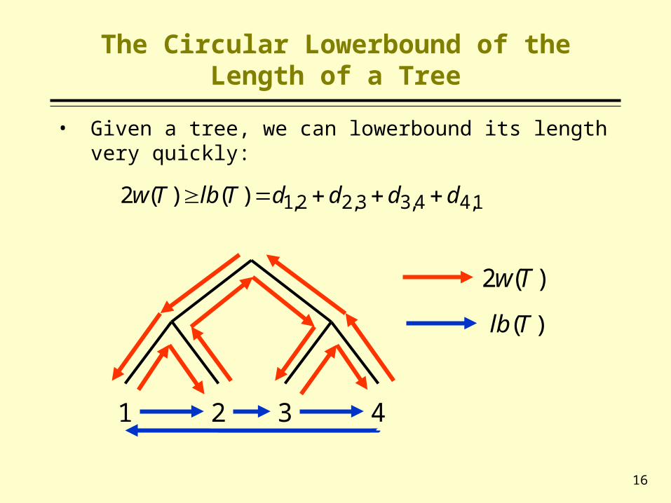
The Circular Lowerbound of the Length of a Tree
• Given a tree, we can lowerbound its length very quickly:
1 2 3 4
1,44,33,22,1)()(2 ddddTlbTw
)(2 Tw
)(Tlb
17
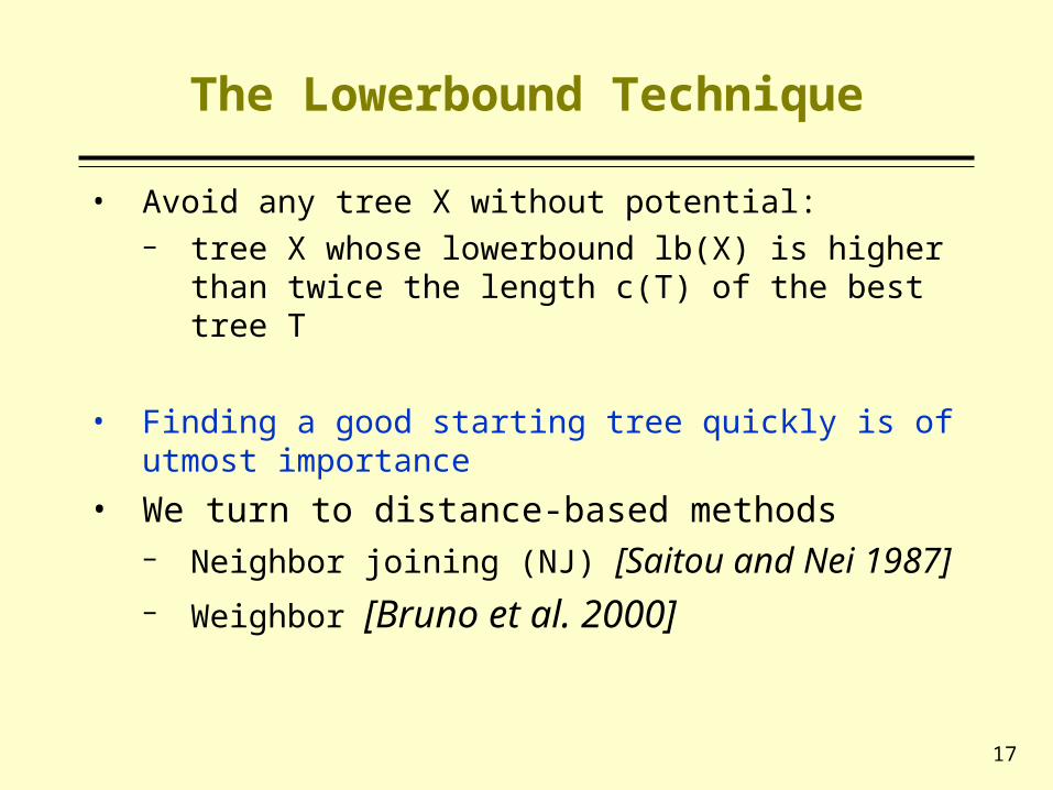
The Lowerbound Technique
• Avoid any tree X without potential:− tree X whose lowerbound lb(X) is higher than
twice the length c(T) of the best tree T
• Finding a good starting tree quickly is of utmost importance
• We turn to distance-based methods− Neighbor joining (NJ) [Saitou and Nei 1987]− Weighbor [Bruno et al. 2000]

18
Additive Distance Matrix and True Evolutionary Distance (T.E.D.)
S2 S3 S4 S5
S1 0 9 15 14 17S2 0 14 13 16S3 0 13 16S4 0 13 13
75
4
5
8
S1
S2
S3
S4
S5
S1
S5 0
Theorem [Waterman et al. 1977] Given an m×m additive distance matrix, we can reconstruct a tree realizing the distance in O(m2) time.

19
Error Tolerance of Neighbor Joining
Theorem [Atteson 1999]Let {Dij} be the true evolutionary distances, and {dij} be the estimated distances for T. Let be the length of the shortest edge in T. If for all taxa i,j, we have
then neighbor joining returns T.
2
1|| ijij dD

20
BP and INV
INV vs K(120 genes)
(K: Actual number of inversions) (Inversion-only evolution)
BP/2 vs K

21
NJ(BP) [Blanchette, Kunisawa, Sankoff 1999] and NJ(INV)
120 genes, 160 leavesUniformly Random Tree
Transpositions/inverted transpositions only
Inversion only

22
Estimate True Evolutionary DistancesUsing BP
BP/2 vs K (120 genes)
(K: Actual number of inversions) (Inversion-only evolution)
To use the scatter plot to estimate the actual number of events (K):
1. Compute BP/2
2. From the curve, look up the corresponding valueof K
(1)
(2)

23
True Evolutionary Distance (t.e.d.) Estimators for Gene Order Data
T.E.D. Estimator
Exact-IEBP [WABI’01]
Approx-IEBP [STOC’01]
EDE [ISMB’01]
Based on the Expectation of
Breakpoint distance (Exact)
Breakpoint distance (Approx.)
Inversion distance (Approx.)
Derivation Analytical Analytical Empirical
Model knowledge
Required Required Inversion-only
IEBP: Inverting the Expected BreakPoint distanceEDE: Empirically Derived Estimator

24
True Evolutionary Distance Estimators
Exact-IEBP vs K(120 genes)
(K: Actual number of inversions) (Inversion-only evolution)
BP vs K

25
Variance of True Evolutionary Distance Estimators
• There are new distance-based phylogeny reconstruction methods (though designed for DNA sequences) − Weighbor [Bruno et al. 2000]
These methods use the variance of good t.e.d.’s, and yield more accurate trees than NJ.
• Variance estimates for the t.e.d.s [Wang WABI’02]− Weighbor(IEBP),
Weighbor(EDE) K vs Exact-IEBP (120 genes)

26
Using T.E.D. Helps
120 genes160 leavesUniformly random treeTranspositions/invertedtranspositions only(180 runs per figure)
5%
27
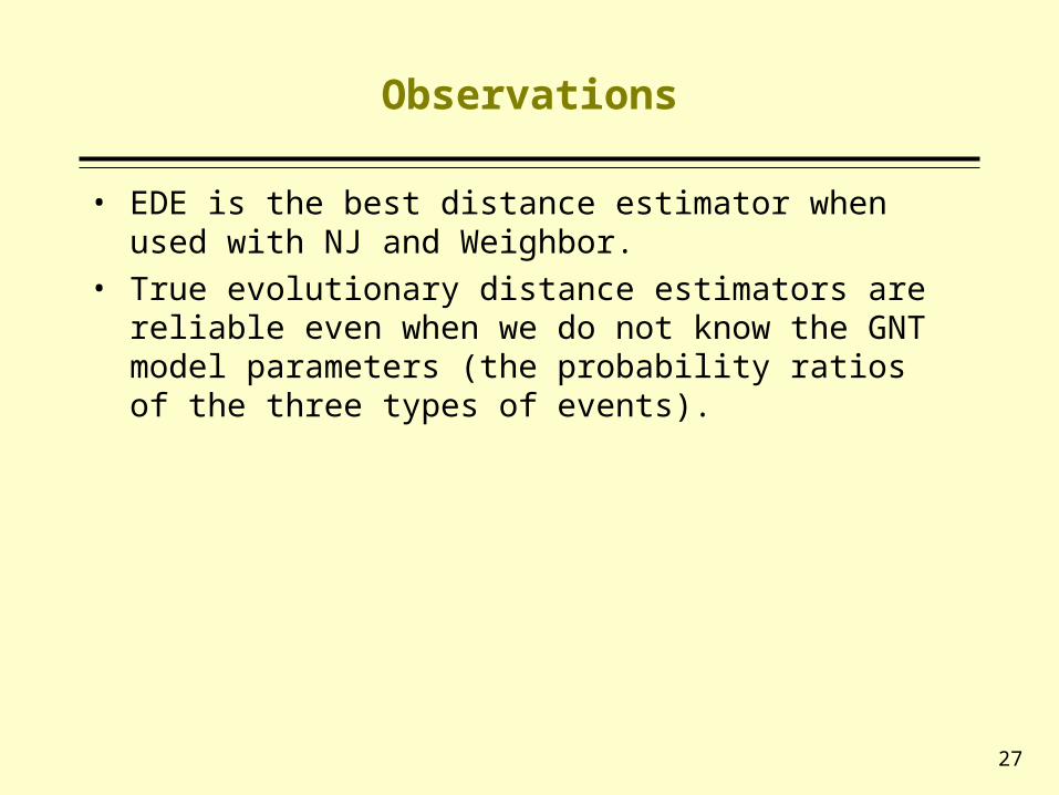
Observations
• EDE is the best distance estimator when used with NJ and Weighbor.
• True evolutionary distance estimators are reliable even when we do not know the GNT model parameters (the probability ratios of the three types of events).

28
Outline
• Genome rearrangement evolution• Genome rearrangement phylogeny reconstruction• Application• Other methods• Future research

29
Percentage of Trees Eliminated Through Bounding [ISMB’01]
edge length=2
# taxa 10 20 40 80 160
10 0 0 0 1% 1%
20 0 80% 91% 1% 1%
40 91% 100% 100% 100% 100%
80 99% 100% 100% 100% 100%
160 100% 100% 100% 100% 100%
320 100% 100% 100% 100% 100%
#genes Uses NJ(EDE) as starting tree

30
Campanulaceae cpDNA
• 13 taxa (tobacco as outlier)• 105 gene segments• GRAPPA finds 216 trees with shortest breakpoint
length (out of 654,729,075 trees)
• Running Time:− BPAnalysis takes 2 centuries on a Sun
workstation− GRAPPA takes 1.5 hours on a 512-node
supercluster− About 2300-fold speedup on a single node

31
Campanulaceae [Moret et al. ISMB 2001]
Strict consensus of 216 optimal trees found by GRAPPA
Tob
acco
Pla
tyco
don
Cya
nant
hus
Cod
onop
sis M
erci
era
Wah
lenb
ergi
a
Tri
odan
is
Asy
neum
a Leg
ousi
a
Sym
phan
dra
Ade
noph
ora
Cam
panu
la Tra
chel
ium
6 out of 10 max. edges found

32
Outline
• Genome rearrangement evolution• Genome rearrangement phylogeny reconstruction• Application• Other methods• Future research
33
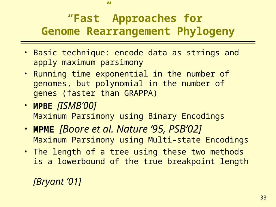
“Fast” Approaches for Genome Rearrangement Phylogeny
• Basic technique: encode data as strings and apply maximum parsimony
• Running time exponential in the number of genomes, but polynomial in the number of genes (faster than GRAPPA)
• MPBE [ISMB’00]Maximum Parsimony using Binary Encodings
• MPME [Boore et al. Nature ’95, PSB’02]Maximum Parsimony using Multi-state Encodings
• The length of a tree using these two methods is a lowerbound of the true breakpoint length [Bryant ’01]
34
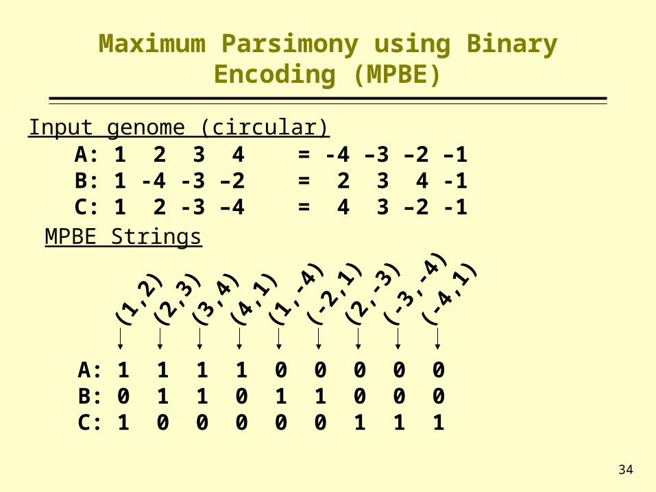
Maximum Parsimony using Binary Encoding (MPBE)
A: 1 2 3 4 = -4 –3 –2 –1B: 1 -4 -3 –2 = 2 3 4 -1C: 1 2 -3 –4 = 4 3 –2 -1
MPBE Strings
Input genome (circular)(1,2)
(2,3)
(3,4)
(4,1)
(1,-4)
(-2,1)
(2,-3)
(-3,-4)
(-4,1)
A: 1 1 1 1 0 0 0 0 0B: 0 1 1 0 1 1 0 0 0C: 1 0 0 0 0 0 1 1 1

35
Maximum Parsimony using Multistate Encoding (MPME)
MPME Strings
Input genome (circular)
A: 2 3 4 1 –4 –1 –2 -3B: -4 3 4 –1 2 1 –2 -3C: 2 –3 -2 3 4 –1 -4 1
1 2 3 4 -1 –2 –3 -4
A: 1 2 3 4 = -4 –3 –2 –1B: 1 -4 -3 –2 = 2 3 4 -1C: 1 2 -3 –4 = 4 3 –2 -1
We use PAUP to solve Maximum Parsimony
=> Constraint: number of states per site cannot exceed 32

36
NJ vs MP (120 genes, 160 genomes)
All three event types equiprobable(datasets that exceed 32-state limit for MPME are dropped)

37
Inversion Phylogeny
• Inversion median has higher running time than breakpoint median
• Inversion phylogeny overall has shorter running time than breakpoint phylogeny, and returns more accurate trees [Moret et al. WABI ’02]

38
• Disk-Covering Method: divide the original problem into subproblems [Huson, Nettles, Parida, Warnow and Yooseph, 1998]
• Uses inversion distance• DCM-GRAPPA: can now process thousands of
genomes, each having hundreds of genes
DCM-GRAPPA [Moret & Tang 2003]

39
Ongoing and Future Research
• Genome rearrangement phylogeny with unequal gene content (duplications, deletions, etc.)
• Non-uniform genome rearrangement models(Segment-length dependent model, hotspots)

40
Acknowledgements
• University of Texas Tandy Warnow (Advisor) Robert K. Jansen Stacia Wyman Luay Nakhleh Usman Roshan Cara Stockham Jerry Sun
• University of New Mexico Bernard M.E. Moret David Bader Jijun Tang Mi Yan
• Central Washington University Linda Raubeson

41
PhylolabDepartment of Computer Sciences
University of Texas at Austin
Please visit us athttp://www.cs.utexas.edu/users/phylo/


