
Notes on “General Relativity” (Wald, 1984)
Robert B. Scott,1,2∗
1Institute for Geophysics, Jackson School of Geosciences, The University of Texas at Austin,
Austin, Texas, USA2Department of Physics, University of Brest,
Brest, France
∗To whom correspondence should be addressed; E-mail: [email protected].
March 10, 2012

2

Part I
Fundamentals
3


Chapter 1
Introduction
5

6
Chapter 2
Manifolds and Tensor Fields
2.5 Problems
Problem 1 (a) Show that the overlap functions, discussed in § 2.1 in theproof that the 2-sphere is a manifold, are smooth.
The overlap functions are
f±i ◦ (f±j )−1
where f±i is the projection, for example:
f+1 (x, y, z) = (y, z)
on the domain x > 0. Let’s construct a particular overlap function. For
f+2 (x, y, z) = (x, z)
This projects the hemisphere y > 0 onto the x − z plane. Its inverse takespoints in the x− z plane and projects them back onto the 2-sphere surface:
(f+2 )−1(x, z) = (x,+
√1− x2 − z2, z)
where the positive root corresponds to the domain of f+2 . The composite
with f+1 will project these points onto the y − z plane.
f+1 ◦ (f+
2 )−1(x, z) = (√
1− x2 − z2, z)
7

8
We must show that this function is C∞.
Problem 1 (b) Construct two coordinate systems that cover the 2-sphere.
We use spherical coordinates being careful to avoid the singularities atthe poles. But remember that the charts must map from open subsets of themanifold into open subsets of <n, so we cannot just use the two hemispheressince the Equator would be omitted.
For the first coordinate system, ψ1, use spherical coordinates and avoidthe poles by restricting π/6 < θ < 5π/6. Then the subset of the manifold S2
that’s covered is
O1 =
{(x1, x2, x3) ∈ S2
∣∣∣∣∣−√
3
2< x3 <
√3
2
}So the first chart
ψ1 : O1 → U1 ⊂ <2
is specifically
ψ1(x1, x2, x3) = (θ, φ) (2.1)
with
θ = arccos(z)
φ = arctan(y/x) (2.2)
To fill the holes near the poles, we construct another coordinate systemwith a similar chart, ψ2. We simply replace x3 with x1 so that the poles ofthe second spherical coordinate system lie on the x−axis. These cover
O2 =
{(x1, x2, x3) ∈ S2
∣∣∣∣∣−√
3
2< x1 <
√3
2
}and we see our coordinates cover the manifold.
It seems to me that we should also check the regularity of the coordinates,(Faber, 1983, § 1.3), although it wasn’t clear to me that Wald discusses this.This amounts to inverting the function (2.1),
ψ−1(θ, φ) = (x1, x2, x3)
9
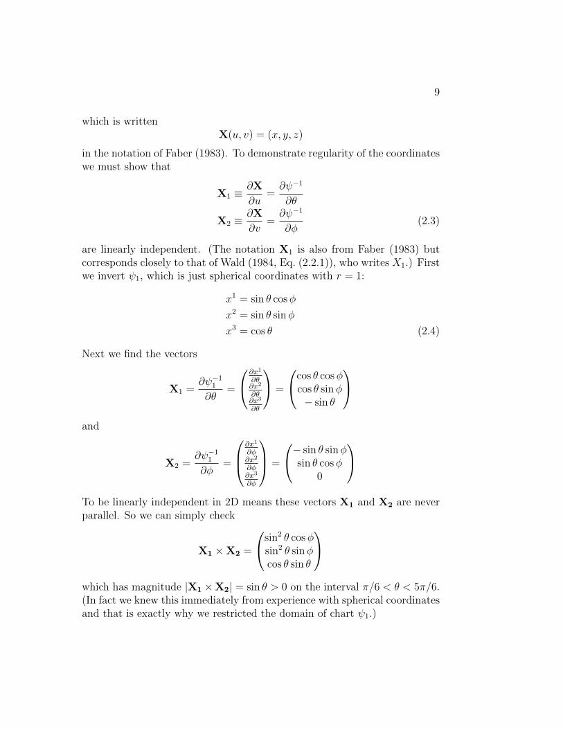
which is writtenX(u, v) = (x, y, z)
in the notation of Faber (1983). To demonstrate regularity of the coordinateswe must show that
X1 ≡∂X
∂u=∂ψ−1
∂θ
X2 ≡∂X
∂v=∂ψ−1
∂φ(2.3)
are linearly independent. (The notation X1 is also from Faber (1983) butcorresponds closely to that of Wald (1984, Eq. (2.2.1)), who writes X1.) Firstwe invert ψ1, which is just spherical coordinates with r = 1:
x1 = sin θ cosφ
x2 = sin θ sinφ
x3 = cos θ (2.4)
Next we find the vectors
X1 =∂ψ−11
∂θ=
∂x1
∂θ∂x2
∂θ∂x3
∂θ
=
cos θ cosφcos θ sinφ− sin θ
and
X2 =∂ψ−11
∂φ=
∂x1
∂φ∂x2
∂φ∂x3
∂φ
=
− sin θ sinφsin θ cosφ
0
To be linearly independent in 2D means these vectors X1 and X2 are neverparallel. So we can simply check
X1 ×X2 =
sin2 θ cosφsin2 θ sinφcos θ sin θ
which has magnitude |X1×X2| = sin θ > 0 on the interval π/6 < θ < 5π/6.(In fact we knew this immediately from experience with spherical coordinatesand that is exactly why we restricted the domain of chart ψ1.)

10
Problem 2 Prove that any smooth function F : <n → R can be writtenin the form equation (2.2.2).
Let’s first make sense of the identity provided in the hint,
F (x)− F (a) = (x− a)
∫ 1
0
F ′[t(x− a) + a]dt (2.5)
Let’s take the antiderivative of the integrand F ′,∫F ′[t(x− a) + a]dt =
1
(x− a)F [t(x− a) + a]
which is easily verified by taking the derivative of both sides with respect tot. And then simply substitute this into the RHS:
F (x)− F (a) = (x− a)
∫ 1
0
F ′[t(x− a) + a]dt
= F [t(x− a) + a]t=1t=0
= F (x)− F (a). (2.6)
So the identity clearly holds when x ∈ <. Now let’s extend it to x ∈ <n.First define a vector
yµ = t(xµ − aµ)
Then by the chain rule,
dF
dt=∑µ
∂F
∂yµdyµ
dt=∑µ
F ′(xµ − aµ)
And
F (x)− F (a) =
∫ 1
0
dF
dtdt
=
∫ 1
0
∑µ
F ′(xµ − aµ)dt
=∑µ
(xµ − aµ)
∫ 1
0
F ′dt
=∑µ
(xµ − aµ)Hµ
(2.7)
11
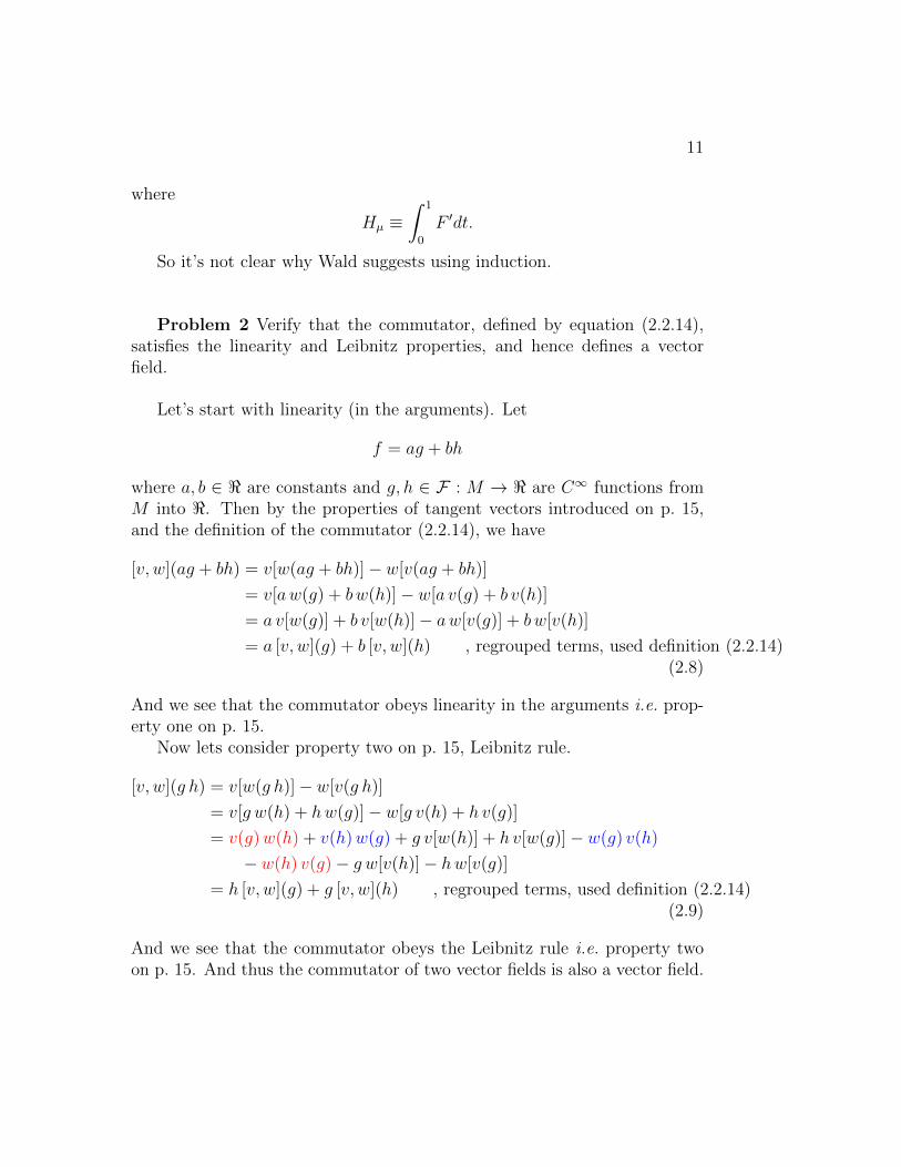
where
Hµ ≡∫ 1
0
F ′dt.
So it’s not clear why Wald suggests using induction.
Problem 2 Verify that the commutator, defined by equation (2.2.14),satisfies the linearity and Leibnitz properties, and hence defines a vectorfield.
Let’s start with linearity (in the arguments). Let
f = ag + bh
where a, b ∈ < are constants and g, h ∈ F : M → < are C∞ functions fromM into <. Then by the properties of tangent vectors introduced on p. 15,and the definition of the commutator (2.2.14), we have
[v, w](ag + bh) = v[w(ag + bh)]− w[v(ag + bh)]
= v[aw(g) + bw(h)]− w[a v(g) + b v(h)]
= a v[w(g)] + b v[w(h)]− aw[v(g)] + bw[v(h)]
= a [v, w](g) + b [v, w](h) , regrouped terms, used definition (2.2.14)(2.8)
And we see that the commutator obeys linearity in the arguments i.e. prop-erty one on p. 15.
Now lets consider property two on p. 15, Leibnitz rule.
[v, w](g h) = v[w(g h)]− w[v(g h)]
= v[g w(h) + hw(g)]− w[g v(h) + h v(g)]
= v(g)w(h) + v(h)w(g) + g v[w(h)] + h v[w(g)]− w(g) v(h)
− w(h) v(g)− g w[v(h)]− hw[v(g)]
= h [v, w](g) + g [v, w](h) , regrouped terms, used definition (2.2.14)(2.9)
And we see that the commutator obeys the Leibnitz rule i.e. property twoon p. 15. And thus the commutator of two vector fields is also a vector field.

12

Part II
Advanced Topics
13

Chapter 10
Initial Value Formulation
Wants to argue that GR admits a well posed initial value problem. For him,this means that it should permit “reasonable specification” of the initial con-ditions, and that Einstein’s equations uniquely predict the future evolution.[emphasis added].
Then he adds two additional conditions for what it takes for the EinsteinEquations to be well posed. Amazingly, we considers sensitivity to initialconditions to render the problem ill-posed:
First, in an appropriate sense, “small changes” in initial datashould produce only correspondingly “small changes” in the so-lution over any fixed compact region of spacetime. If this propertywere not satisfied, the theory would lose essentially all predictivepower, since initial conditions can be measured only to finite ac-curacy. It is generally assumed that the pathological behaviourthat would result from the failure of this property does not occurin physics.
(Wald, 1984, p. 244)
A second condition for the initial value problem to be well-posed is thatchanges to the initial conditions in a region S should only lead to changes inthe casual future of S, that is J+(S). Otherwise, we would have faster thanlight signals.
He will be expressing the Einstein equations as 2nd order hyperbolicsystems. (Other expressions are possible.)
15

16
10.1 Initial Value Formulation of Particles and
Fields
Gives the example of n particles governed by Newtonian mechanics, a systemthat admits an initial value formulation.
Gives the Klein-Gordon equations as another example. Argues that if theinitial conditions are specified with analytic functions, then the Klein-Gordonsystem admits an initial value formulation – that is we can specify arbitraryinitial conditions of φ and its first temporal derivative on a hyper surface ofconstant time Σ0. Then the solution is uniquely determined for later times.He shows that in principle the solution at later times can be written as aTaylor series about the initial time, and one can in principle build all termsin the Taylor series. (In essence because the governing equation gives onethe 3rd derivative in terms of the first, the 4th in terms of the 2nd, etc.
The Cauchy-Kolwaleski, proven in say Courant and Hilbert, states thatthe power series [sounds like a Taylor series to me] solution has a “finite radiusof convergence”. In the theorem they state there is an open neighbourhoodO of the initial time t0 hyper surface such that within O there is a uniqueanalytical solution of the Klein-Gordon equations.
According to Wald, the Cauchy-Kolwaleski theorem is not enough for ourpurposes for two reasons. (1) It doesn’t guarantee the that the map from(analytical) initial conditions to the solution at finite time will be continuous.(2) When the initial conditions are given by analytic functions, then theinitial conditions over the entire initial time t0 hyper surface are determinedby the initial conditions within an open region [because from the informationwithin the open region one could form all the derivatives and then build theTaylor series and describe the analytical function everywhere on the hypersurface.] But then if we change the initial conditions within some openregion we must in fact change the initial conditions everywhere. Apparentlythis violates the causality requirement! Wald says therefore that we mustconsider initial conditions given by non-analytical functions! [This is amazingto me! Personally, I think it means that you cannot arbitrarily change initialconditions.].
Part III
Appendices
17

Chapter 11
Topological Spaces
Compact: Every open cover of a set has a finite sub cover. The open interval(0, 1) in the standard topology of the reals is not compact since it has anopen cover provided by the sets On = (1/n, 1) with n = 2, 3, . . . that doesn’tallow a finite subcover.
THEOREM A.8 A subset of Rn is compact if and only if it is closed andbounded.
19

20

Bibliography
Faber, R. L., 1983: Differential geometry and relativity theory: An Introduc-tion. Marcel Dekker. 255 + X pp.
Wald, R. M., 1984: General Relativity . The University of Chicago Press.
21


