
From the Samuelson Volatility Effect to a Samuelson Correlation Effect: An
Analysis of Crude Oil Calendar Spread Options
Lorenz SCHNEIDERa, Bertrand TAVINa,∗
aEMLYON Business School, Ecully, France
Abstract
We introduce a multi-factor stochastic volatility model based on the CIR/Heston stochastic volatility process.
In order to capture the Samuelson effect displayed by commodity futures contracts, we add expiry-dependent
exponential damping factors to their volatility coefficients. The model leads to stochastic correlation between
the returns of two futures contracts. The pricing of single underlying European options on futures contracts
is straightforward and can incorporate the volatility smile or skew observed in the market. We calculate the
joint characteristic function of two futures contracts in the model in analytic form and use it to price calendar
spread options. We then propose analytical expressions to obtain the copula and copula density directly
from the joint characteristic function of a pair of futures. These expressions are convenient to analyze the
term-structure of dependence between the two futures produced by the model. In an empirical application
we calibrate the model to volatility surfaces of vanilla options on WTI and provide evidence that the model
is able to produce the desired stylized facts in terms of volatility and dependence. In particular, we observe
that the returns of two futures are less dependent the greater the time-interval between their maturities is.
In analogy to the classic Samuelson volatility effect, we call this effect the Samuelson correlation effect.
Keywords: Multi-factor stochastic volatility, Futures curve modelling, Option pricing, Crude oil, Fourier
inversion methods
JEL: C02, G13
1. Introduction
Crude oil is by far the world’s most actively traded commodity. It is usually traded on exchanges in the
form of futures contracts. The two most important benchmark crudes are West Texas Intermediate (WTI),
traded on the NYMEX, and Brent, traded on the ICE. In the S&P Goldman Sachs Commodity Index, WTI
has a weight of 24.71% and Brent a weight of 22.34%, for a combined total of almost half the index. Another
widely quoted index, Jim Rogers’ RICI, has weights of 21% for WTI and 14% for Brent. The crude oil
derivatives market is also the most liquid commodity derivatives market. Popular products are European,
American, Asian, and calendar spread options on futures contracts.
∗Corresponding author: EMLYON Business School, 23 Avenue Guy de Collongue, 69130 Ecully, France. Tel.: +33(0)478337800 Fax: +33 (0)478336169.
Email addresses: [email protected] (Lorenz SCHNEIDER), [email protected] (Bertrand TAVIN)
September 21, 2015

An important empirical feature of crude oil markets is the absence of seasonality, which is in marked
contrast to, say, agricultural commodities markets. A second empirical feature is stochastic volatility of
futures contracts, which is clearly reflected in the oil volatility index (OVX), or “Oil VIX”, introduced on
the CBOE in July 2008. A third feature is known as the Samuelson effect (Samuelson, 1965; Bessembinder
et al., 1996; Brooks, 2012), i.e. the empirical observation that a given futures contract increases in volatility
as it approaches its maturity date. Finally, European and American options on futures tend to show a more
or less strongly pronounced volatility smile, the shape of which depends on the option’s maturity.
European and American options depend on the evolution of just one underlying futures contract. In
contrast to these, calendar spread options have a payoff that is calculated from the difference of two futures
contracts with different maturities. Therefore, a mathematical analysis and evaluation of calendar spread
options must be carried out in a framework that models the joint stochastic behaviour of several futures
contracts.
In this article, we propose a multi-factor stochastic volatility model for the crude oil futures curve. Like
the popular Clewlow and Strickland (1999b,a) models, the model is futures-based, not spot-based, which
means it can exactly match any given futures curve by accordingly specifying the futures’ initial values
without “using up” any of the other model parameters. The variance processes are based on the Cox et al.
(1985) and Heston (1993) stochastic variance process. However, in order to capture the Samuelson effect,
we add expiry dependent exponential damping factors. As in the Heston (1993) model, futures returns
and variances are correlated, so that volatility smiles of American and European options observed in the
market can be closely matched. The instantaneous correlation of the returns of two futures contracts is also
stochastic in our multi-factor model, since it is calculated from the stochastic variances.
Our first result is the calculation of the joint characteristic function of the log-returns of two futures con-
tracts in analytic form. Using this function, calendar spread option prices can be obtained via 1-dimensional
Fourier integration as shown by Caldana and Fusai (2013) or the 2-dimensional Fast Fourier Transform
(FFT) algorithm of Hurd and Zhou (2010). The fast speed of these algorithms is of great importance when
calibrating the model to these products.
Our second result is to describe the dependence structure of two futures prices in terms of copulas
obtained from the joint characteristic function of the model. In many studies, the measure chosen to describe
dependence is Pearson’s rho, which, however, depends on the marginal distributions. In our study, the use
of copulas completely insulates our analysis from the influence of the marginals. Then, via the copula,
dependence and concordance measures such as Spearman’s rho and Kendall’s tau are straightforward to
compute.
Copula functions can also be used to give a rigorous definition of the implied correlation of calendar spread
options. The traditional definition assumes a bivariate Black-Scholes-Merton model for the two underlyings,
which assumes in particular that the marginal distributions are log-normal. In contrast, here, using the
actual marginal distributions of the model, we consider the implied correlation for a given calendar spread
2

option price as the value of the correlation parameter in the bivariate Gaussian copula that reproduces this
price.
In an empirical section we calibrate the two-factor version of our model to market data from three different
dates. We show that the model can fit European and American option prices very closely. The model can
therefore be used by a price maker in a crude oil market to provide consistent and arbitrage free prices to
other market participants. Furthermore, we observe that, for a fixed time-horizon, the returns of two futures
become less dependent as the maturity of the second underlying futures contract increases and moves away
from that of the first underlying contract. In analogy to the classic Samuelson volatility effect, we call this
effect the Samuelson correlation effect.
A detailed exposition of commodity models is given by Clark (2014). One of the most important and still
widely used models is the Black (1976) futures model, which is set in the Black-Scholes-Merton framework.
Contracts with different maturities can have different volatilities in this model, but for each contract the
volatility is constant. Therefore, Black’s model doesn’t capture the Samuelson effect. Also, all contracts are
perfectly correlated in this model, since they are driven by the same Brownian motion.
Clewlow and Strickland (1999b,a) propose one-factor and multi-factor models of the entire futures curve
with deterministic time-dependent volatility functions. A popular specification for these functions is with
exponential damping factors. Since this specification still leads to log-normally distributed futures prices,
there is no volatility smile or skew in this model. In the one-factor model, the instantaneous returns of
contracts with different maturities are perfectly correlated; in the multi-factor model, however, these returns
are not perfectly, but deterministically correlated.
Stochastic volatility models have been proposed by Scott (1987, 1997), Hull and White (1987), Heston
(1993), Bakshi et al. (1997) and Schoebel and Zhu (1999) among others. Christoffersen et al. (2009) study
the stochastic correlation between the stock return and variance in a multi-factor version of the Heston
(1993) model. Duffie et al. (2000) define a general class of jump-diffusions, into which the model presented
in this paper fits. Trolle and Schwartz (2009) introduce a two-factor spot based model, with, in addition,
two stochastic volatility factors as well as two stochastic factors for the forward cost-of-carry. The main
focus of their study is on unspanned stochastic volatility of single-underlying options on futures contracts.
Spread options have been well studied in a two-factor Black-Scholes-Merton framework. Margrabe (1978)
gives an exact formula when the strike K equals zero, and Kirk (1995), Carmona and Durrleman (2003),
Bjerksund and Stensland (2011) and Venkatramanan and Alexander (2011) give approximation formulas
for any K. Caldana and Fusai (2013) have recently proposed a very fast one-dimensional Fourier method
that extends the approximation given by Bjerksund and Stensland (2011) to any model for which the joint
characteristic function is known.
The rest of the paper proceeds as follows. In Section 2 we define the proposed model and provide the
associated joint characteristic function. Section 3 deals with spread options and the structure of dependence
produced by the model. Section 4 presents an empirical analysis based on different market situations. Section
3
5 concludes.
2. A Model with Stochastic Volatility for Crude Oil Futures
2.1. The Financial Framework and the Model
We begin by giving a mathematical description of our model under the risk-neutral measure Q. Let n ≥ 1
be an integer, and let B1, ..., B2n be Brownian motions under Q. Let Tm be the maturity of a given futures
contract. The futures price F (t, Tm) at time t, 0 ≤ t ≤ Tm, is assumed to follow the stochastic differential
equation (SDE)
dF (t, Tm) = F (t, Tm)n∑
j=1
e−λj(Tm−t)√
vj(t)dBj(t), F (0, Tm) = Fm,0 > 0. (1)
The processes vj , j = 1, ..., n, are CIR/Heston square-root stochastic variance processes assumed to follow
the SDE
dvj(t) = κj (θj − vj(t)) dt+ σj
√
vj(t)dBn+j(t), vj(0) = vj,0 > 0. (2)
For the correlations, we assume
〈dBj(t), dBn+j(t)〉 = ρjdt,−1 < ρj < 1, j = 1, ..., n, (3)
and that otherwise the Brownian motions Bj , Bk, k 6= j, j+n, are independent of each other. As we will see,
this assumption has as a consequence that the characteristic function factors into n separate expectations.
For fixed Tm, the futures log-price lnF (t, Tm) follows the SDE
d lnF (t, Tm) =
n∑
j=1
(
e−λj(Tm−t)√
vj(t)dBj(t)−1
2e−2λj(Tm−t)vj(t)dt
)
, lnF (0, Tm) = lnFm,0. (4)
Integrating (4) from time 0 up to a time T, T ≤ Tm, gives
lnF (T, Tm)− lnF (0, Tm) =
n∑
j=1
∫ T
0
e−λj(Tm−t)√
vj(t)dBj(t)−1
2
n∑
j=1
∫ T
0
e−2λj(Tm−t)vj(t)dt. (5)
We define the log-return between times 0 and T of a futures contract with maturity Tm as
Xm(T ) := ln
(
F (T, Tm)
F (0, Tm)
)
.
In the following, the joint characteristic function φ of two log-returns X1(T ), X2(T ) will play an important
role. For u = (u1, u2) ∈ C2, φ is given by
φ(u) = φ(u;T, T1, T2) = EQ
[
exp
(
i
2∑
k=1
ukXk(T )
)]
. (6)
The joint characteristic function Φ of the futures log-prices lnF (T, T1), lnF (T, T2) is then given by
Φ(u) = exp
(
i
2∑
k=1
uk lnF (0, Tk)
)
· φ(u). (7)
4

Note that futures prices in our model are not mean-reverting, and that the log-price lnF (t, Tm) at time t
and the log-return lnF (T, Tm)− lnF (t, Tm) are independent random variables. In the following proposition,
we show how the joint characteristic function φ is given by a system of two ordinary differential equations
(ODE).
Proposition 1. The joint characteristic function φ at time T ≤ T1, T2 for the log-returns X1(T ), X2(T ) of
two futures contracts with maturities T1, T2 is given by
φ(u) = φ(u;T, T1, T2)
=
n∏
j=1
exp
(
iρj
σj
{
κjθj
λj
(fj,1(u, 0)− fj,1(u, T ))− fj,1(u, 0)vj(0)
})
exp (Aj(0, T )vj(0) +Bj(0, T )) ,
where
fj,1(u, t) =
2∑
k=1
uke−λj(Tk−t), fj,2(u, t) =
2∑
k=1
uke−2λj(Tk−t),
qj(u, t) = iρjκj − λj
σj
fj,1(u, t)−1
2(1− ρ2j )f
2j,1(u, t)−
1
2ifj,2(u, t),
and the functions Aj : (t, T ) 7→ Aj(t, T ) and Bj : (t, T ) 7→ Bj(t, T ) satisfy the two differential equations
∂Aj
∂t− κjAj +
1
2σ2jA
2j + qj = 0,
∂Bj
∂t+ κjθjAj = 0,
with Aj(T, T ) = iρj
σjfj,1(u, T ), Bj(T, T ) = 0.
The single characteristic function φ1 at time T ≤ T1 for the log-return X1(T ) of a futures contract with
maturity T1 is given by setting u2 = 0 in the joint characteristic function.
The statement regarding the single characteristic function immediately follows from the definition of the
joint characteristic function. The joint characteristic function is calculated in Section 6.
In the next proposition, we show how this ODE system can be solved analytically. A closed form
expression for Aj is found thanks to a computer algebra software and Bj is proportional to the integral of
Aj on [0, T ].
Proposition 2. Dropping the references to j, the function A : (t, T ) 7→ A(t, T ) is given in closed form as
A(t, T ) =1√2zσ
· ((M−(t)−M+(t))X0 +X1U
+(t))C1 − 2 (M+(t)X0 −X1U+(t)) (C3 − iC2)e
λt
M+(t)X0 −X1U+(t)
+1
σ2· ((κ− λ)M+(t) + (κ+ λ)M−(t))X0 − ((κ− λ)U+(t)− 2λU−(t))X1
M+(t)X0 −X1U+(t),
with z =√C2 + iC3 and C1, C2, C3 constants with respect to t, defined as
C1 = ρκ− λ
σ
2∑
k=1
uke−λTk , C2 = −1
2(1− ρ2)
(
2∑
k=1
uke−λTk
)2
, C3 = −1
2
2∑
k=1
uke−2λTk ,
5
X0 = 2Y U+(T ) + 4zλU−(T ),
X1 = 2YM+(T )− 2
(
z(λ+ κ) + σ√2C1
2
)
M−(T ),
Y = σ√2
(
C1
2− ieλTC2 + eλTC3
)
− z (κ− λ− iρf1(T )σ) ,
M±(t) = M
(
κz − σ√2
2 C1
2zλ± 1
2,κ+ λ
λ,σ√2
λizeλ t
)
,
U±(t) = U
(
κz − σ√2
2 C1
2zλ± 1
2,κ+ λ
λ,σ√2
λizeλ t
)
.
The functions M and U are the confluent hypergeometric functions.
A description of M and U functions as well as useful properties for their implementation can be found in
Appendix A.
The models of Clewlow and Strickland (1999b,a) are useful benchmarks, so we give a description of them
and calculate their joint characteristic function. In the risk-neutral measure Q, the futures price F (t, Tm) is
modelled with deterministic time-dependent volatility functions σj(t, Tm):
dF (t, Tm) = F (t, Tm)
n∑
j=1
σj(t, Tm)dBj(t), (8)
where B1, ..., Bn are independent Brownian motions. A popular specification for the volatility functions is
σj(t, Tm) := e−λj(Tm−t)σj (9)
for fixed parameters σj , λj ≥ 0, so that the volatility of a contract a long time away from its maturity is
damped by the exponential factor(s).
Proposition 3. In the Clewlow and Strickland model defined by (8) and (9), the joint characteristic function
φ at time T ≤ T1, T2 for the log-returns X1(T ), X2(T ) of two futures contracts with maturities T1, T2 is given
by
φ(u) = φ(u;T, T1, T2)
=
n∏
j=1
exp
(
−σ2j
4λj
(e2λjT − 1){
i(u1e−2λjT1 + u2e
−2λjT2) + (u1e−λjT1 + u2e
−λjT2)2}
)
.
The single characteristic function φ1 at time T ≤ T1 for the log-return of a futures contract with maturity
T1 is given by setting u2 = 0 in the joint characteristic function.
We prove this result in Section 6.
This result can also be used to add non-stochastic volatility factors to the model by multiplying the joint
characteristic function of Proposition 1 with one or more factors from Proposition 3. Since each “Clewlow-
Strickland” factor depends on only two parameters λj and σj , it does not add a significant burden to the
calibration to market data, while allowing for increased flexibility when fitting the model to the observed
volatility term structure.
6

2.2. Pricing Vanilla Options
European options on futures contracts can be priced using the Fourier inversion technique as described in
Heston (1993) and Bakshi and Madan (2000), or the FFT algorithm of Carr and Madan (1999). Alternatively,
they can be priced by Monte Carlo simulation using discretizations of (1) (Euler scheme) or (4) (Log-Euler
scheme) and of (2).
Let K denote the strike and T the maturity of a European call option on a futures contract F with
maturity Tm ≥ T , and let the single characteristic function Φ1 of the futures log-price lnF (T, Tm) be given
by Φ1(u) = eiu lnF (0,Tm)φ1(u). In the general formulation of Bakshi and Madan (2000), the numbers
Π1 :=1
2+
1
π
∫ ∞
0
ℜ[
e−iu lnKΦ1(u− i)
iuΦ1(−i)
]
du, (10)
Π2 :=1
2+
1
π
∫ ∞
0
ℜ[
e−iu lnKΦ1(u)
iu
]
du, (11)
represent the probabilities of F finishing in-the-money at time T in case the futures F itself or a risk-
free bond is used as numeraire, respectively. The price C of a European call option is then obtained
with the formula C = e−rT (F (0, T1)Π1 −KΠ2) . European put options can be priced via put-call parity
C − P = e−rT (F (0, T1)−K).
American call and put options can be evaluated via Monte-Carlo simulation using the method of Longstaff
and Schwartz (2001). Alternatively, the early exercise premium can be approximated with the formula of
Barone-Adesi and Whaley (1987). Trolle and Schwartz (2009) address the issue of estimating European
prices from American prices. Chockalingam and Muthuraman (2011) study the problem of pricing American
options with stochastic volatility models, including the Heston model; quite possibly their method can be
adapted to the model presented here.
A typical WTI volatility surface displays high implied volatilities at the short end and low implied
volatilities at the long end. This is in line with the Samuelson effect. Furthermore, there is usually a
strongly pronounced smile at the short end, and a weak smile at the long end.
3. Calendar Spread Options and Analysis of Dependence
In this section we review the pricing of calendar spread options and the notion of implied correlation.
Then we introduce analytic results to obtain the copula function and its density from the joint characteristic
function.
3.1. Calendar Spread Options written on WTI futures
Calendar spread options (CSO) are very popular options in commodities markets. There are two types of
these options: calendar spread calls (CSC) and calendar spread puts (CSP). Like spread options in equities
derivatives markets, their payoff depends on the price difference of two underlying assets. A call spread option
on two equity shares S1 and S2 gives the holder, at time T , the payoff max (S1(T )− S2(T )−K, 0) , and a
7
put the payoff max (K − (S1(T )− S2(T )) , 0) . In the case of calendar spread options, the two underlyings
are two futures contracts on the same commodity, but with different maturities T1 and T2. Examples of
CSOs are the NYMEX calendar spread options on WTI crude oil. A WTI CSC (CSP) represents an option
to assume a long (short) position in the first expiring futures contract in the spread and a short (long)
position in the second contract. There are also so-called financial CSOs traded on the NYMEX, which are
cash settled. For pricing purposes we will not distinguish between these two settlement types in this paper.
There is usually very good liquidity on 1-month spreads (for which T2 − T1 = 1 month), whereas options on
2, 3, 6 and 12-month spreads are less liquid.
Let two futures maturities T1, T2, an option maturity T , and a strike K (which is allowed to be negative)
be fixed. Then the payoffs of calendar spread call and put options, CSC and CSP , are respectively given
by
CSC(T ) = (F (T, T1)− F (T, T2)−K)+, (12)
CSP (T ) = (K − (F (T, T1)− F (T, T2)))+. (13)
To evaluate such options with a pricing model, the discounted expectation of the payoff must be calculated
in the risk-neutral measure. Assuming a continuously-compounded risk-free interest rate r, we have at time
t0 = 0:
CSC(0, T, T1, T2,K) = e−rTE0
[
(F (T, T1)− F (T, T2)−K)+]
, (14)
CSP (0, T, T1, T2,K) = e−rTE0
[
(K − (F (T, T1)− F (T, T2)))+]
. (15)
Note that there is a model-independent put-call parity for calendar spread options:
CSC(0)− CSP (0) = e−rT (F (0, T1)− F (0, T2)−K) . (16)
Apart from Monte-Carlo simulation (where simulation of the CIR/Heston process is well-understood),
we are aware of three efficient methods to price spread options. The first two are suitable when the joint
characteristic function is available. The third one is more direct but needs the marginals and joint distribution
function of the underlying futures.
The formula of Bjerksund and Stensland (2011) for a joint Black-Scholes-Merton model is generalized by
Caldana and Fusai (2013) to models for which the joint characteristic function is known. Strictly speaking,
these methods give a lower bound for the spread option price. However, our tests lead us to agree with
the above authors that this lower bound is very close to the actual price (typically the first three digits
after the comma are the same), and we therefore regard this lower bound as the spread option’s price
itself. Furthermore, in case K = 0 the formula is exact (exchange option case). This method relies on a
one-dimensional Fourier inversion and appears to be the most suitable to our model and setup. We give
additional details on its implementation in Appendix B.
An alternative method that also works with the joint characteristic function of the log-returns has been
proposed by Hurd and Zhou (2010). In their paper, the transform of the calendar spread payoff function
8

with a strike of K = 1 is calculated analytically, and the price of the corresponding option is then deduced
from this result. This method needs a double integral to be evaluated numerically using the two-dimensional
Fast Fourier Transform (2d FFT).
Methods working with distribution functions instead of characteristic functions are also available to price
calendar spread options. The most direct approach is to evaluate a double integral of the payoff function
times the joint density of the two underlying futures contracts. However, we can write calendar spread option
prices as single integrals over the marginal and joint distribution functions. The calendar spread call and
put option prices are given, at t = 0 and for K ≥ 0, by
CSC(0,K, T, T1, T2) =
∫ +∞
0
(G2(x, T, T2)−G(x, x+K,T, T1, T2)) dx, (17)
CSP (0, T, T1, T2,K) =
∫ +∞
0
(G1(x+K,T, T1)−G(x, x+K,T, T1, T2)) dx, (18)
where G1 and G2 are the marginal distribution functions of X1 and X2, respectively, and G is their joint
distribution function. The case K < 0 is treated as a calendar spread option written on the reverse spread
F (T, T2)− F (T, T1) with the opposite strike −K.
In our model, the distribution functions involved in (17) and (18) are not readily available. However, it
is possible to calculate G1 and G2 from the joint characteristic function φ of (X1, X2) using direct inversion
formulas given by
G1(x, T, T1) =eax
2π
∫ +∞
−∞e−iuxφ(u+ ia, 0, T, T1, T2)
a− iudu, (19)
G2(x, T, T2) =eax
2π
∫ +∞
−∞e−iuxφ(0, u+ ia, T, T1, T2)
a− iudu, (20)
with a proper choice of the smoothing parameter a > 0. A detailed proof of these inversion results can be
found in Le Courtois and Walter (2015). The joint distribution function G can be recovered in a similar way
using a direct two-dimensional inversion formula.
Lemma 4.
G(x1, x2, T, T1, T2) =ea1x1+a2x2
4π2
∫ +∞
−∞
∫ +∞
−∞e−i(u1x1+u2x2)
φ(u1 + ia1, u2 + ia2, T, T1, T2)
(a1 − iu1)(a2 − iu2)du1du2. (21)
The proof of this expression follows along the same lines as the one for the univariate case given by Le
Courtois and Walter (2015). It is given in Section 6.
Inversion formulas (19),(20) and (21) are suitable for the use of FFT methods in one and two dimensions.
We refer to Appendix D and Appendix E for more details about the implementation of these formulas.
For completeness, we note that the joint density g(., T, T1, T2) of X(T ) = (X1(T ), X2(T )) is given by
g(x1, x2, T, T1, T2) =1
4π2
∫ +∞
−∞
∫ +∞
−∞e−i(u1x1+u2x2)φ(u1, u2, T, T1, T2)du1du2. (22)
9

The marginal densities g1(., T, T1) and g2(., T, T2) of X1(T ) and X2(T ), respectively, are recovered as
g1(x1, T, T1) =1
π
∫ +∞
0
Re[
e−iux1φ(u, 0, T, T1, T2)]
du, (23)
g2(x2, T, T2) =1
π
∫ +∞
0
Re[
e−iux2φ(0, u, T, T1, T2)]
du. (24)
3.2. Implied Correlation for Calendar Spread Options
Given the price of a CSO, it is possible to extract an implied correlation reflecting the level of dependence
embedded in the given price. This implied correlation can be defined as the parameter of the Gaussian copula
that reproduces the observed price. It exists whenever the observed price is free of arbitrage. This copula-
based definition has the advantage that it disentangles the impact of the marginals on the price of a CSO
from the dependence structure.
For ρ ∈ [−1, 1], we denote by CGρ the bivariate Gaussian copula with parameter ρ. Special cases are
CGρ=+1 (u1, u2) = C+ (u1, u2) and CG
ρ=−1 (u1, u2) = C− (u1, u2), for (u1, u2) ∈ [0, 1]2, where C+ and C−
are the usual upper and lower Frechet-Hoeffding bounds. For definitions and general theory about copula
functions we refer to Nelsen (2006) and Mai and Scherer (2012).
When the chosen dependence structure is given by a Gaussian copula with correlation parameter ρ, and
its marginals are G1 and G2, the price of the strike K calendar spread call option is denoted by CSCG and
is given by, for ρ ∈]− 1,+1[,
CSCG(0, T, T1, T2,K, ρ) = e−rT
∫ +∞
0
(
G1(x, T )− CGρ (G1(x, T ), G2(x+K,T ))
)
dx, (25)
and, for ρ = ±1
CSCG(0, T, T1, T2,K, ρ = +1) = CSC+0 (K) = e−rT
∫ 1
0
(
G−12 (u, T )−G−1
1 (u, T )−K)+
du,
CSCG(0, T, T1, T2,K, ρ = −1) = CSC−0 (K) = e−rT
∫ 1
0
(
G−12 (u, T )−G−1
1 (1− u, T )−K)+
du,
where CSC+ and CSC− denote the prices obtained for the calendar spread option when the chosen depen-
dence structures are respectively C+ and C−.
The implied correlation ρ∗ is now defined as the value of the correlation parameter in (25) that reproduces
the observed market price. For a CSP, it is defined via put-call parity (16). One can easily show that for
any arbitrage-free price, ρ∗ exists and is unique. Note that implied correlation depends on both the strike
and the maturity of the CSO. By analogy with implied volatility, these phenomena are referred to as implied
correlation smile (or frown) and implied correlation term-structure.
3.3. Analysis of the Dependence Structure Between two Futures
We now turn to the analysis of the dependence between futures prices at a future time horizon in by our
model. As we have seen, it is possible to recover the marginal and joint density and distribution functions
from the joint characteristic function. Here we show how to obtain the copula function and its density.
10
Let C(., T ) denote the copula function between the log-returns X1(T ) and X2(T ) of two futures contracts.
Note that, expressed as a copula (or a copula density), the dependence between the log-returns is the same
as the dependence between the prices themselves. For readability, we drop the explicit reference to T1 and
T2 in the expressions in the remainder of the section.
Proposition 5. The copula function C describing the dependence between X1(T ) and X2(T ) and the cor-
responding copula density c can be recovered, for (v1, v2) ∈ [0, 1]2, as
C(v1, v2, T ) =ea1G
−1
1(v1,T )+a2G
−1
2(v2,T )
4π2
·∫ +∞
−∞
∫ +∞
−∞
e−i(u1G−1
1(v1,T )+u2G
−1
2(v2,T ))φ(u1 + ia1, u2 + ia2, T )
(a1 − iu1)(a2 − iu2)du1du2, (26)
c(v1, v2, T ) =
∫ +∞−∞
∫ +∞−∞ e−i(u1G
−1
1(v1,T )+u2G
−1
2(v2,T ))φ(u1, u2, T )du1du2
∫ +∞−∞ e−iuG−1
1(v1,T )φ(u, 0, T )du
∫ +∞−∞ e−iuG−1
2(v2,T )φ(0, u, T )du
, (27)
where G−11 and G−1
2 are the inverse cumulative distribution functions of X1(T ) and X2(T ).
We prove this result in Section 6.
The dependence structure created by the model between X1(T ) and X2(T ) is entirely described by the
copula function C(., T ). This copula function depends on the chosen time horizon T , and we therefore
have a term-structure of dependence that can be obtained from φ. The indexing by T of the copula C
should be understood as a time-horizon, since it describes, seen from t = 0, the distribution of the random
vector (G1(X1(T ), T ), G2(X2(T ), T )). The chosen model produces a term-structure of dependence (i.e. a
term-structure of copulas) which should not be confused with a time dependent copula.
Figure 1 plots the copula function and copula density between two futures prices obtained with the SV2F
model and parameters as given in Table 1. The chosen futures respective maturities are T1 = 0.25 years and
T2 = 0.75 years, and the chosen time horizon is T = 0.25 years.
11

0
0.2
0.4
0.6
0.8
1
0
0.2
0.4
0.6
0.8
1
0
0.2
0.4
0.6
0.8
1
u1
u2 u
1
u2
0.1 0.2 0.3 0.4 0.5 0.6 0.7 0.8 0.9
0.1
0.2
0.3
0.4
0.5
0.6
0.7
0.8
0.9
0.1
0.2
0.3
0.4
0.5
0.6
0.7
0.8
0.9
0
0.2
0.4
0.6
0.8
1
0
0.2
0.4
0.6
0.8
1
0
5
10
15
20
25
30
35
u1
u2 u
1
u2
0.1 0.2 0.3 0.4 0.5 0.6 0.7 0.8 0.9
0.1
0.2
0.3
0.4
0.5
0.6
0.7
0.8
0.9
5
10
15
20
25
30
Figure 1: Copula function and copula density representing the dependence structure between F (T, T1) and F (T, T2), for
T = T1 = 0.25 years and T2 = 0.75 years, obtained with SV2F model and parameters as given in Table 1.
κ1 κ2 θ1 θ2 ρ1 ρ2 σ1 σ2 v1(0) v2(0) λ1 λ2
1.00 1.00 0.16 0.09 0.00 0.00 0.25 0.20 0.16 0.09 0.10 2.00
Table 1: Model parameters used to illustrate the dependence structure between two futures in Section 3.3.
To assess the dependence between X1(T ) and X2(T ) with a single number instead of a function one can
rely on concordance and dependence measures. Two well-known concordance measures are Kendall’s tau
and Spearman’s rho. For (X1(T ), X2(T )) these measures are denoted by τK(X1, X2, T ) and S(X1, X2, T ),
respectively. Two well-known dependence measures are Schweizer-Wolf’s sigma and Hoeffding’s phi. For
(X1(T ), X2(T )) these measures are denoted by σSW (X1, X2, T ) and ΦH(X1, X2, T ), respectively. Concor-
dance and dependence measures can be expressed as double integrals on the unit square [0, 1]2 of the copula of
(X1(T ), X2(T )) and its density. We refer to Nelsen (2006) for statements of these expressions and properties
of these measures.
4. Calibration to Market Data and Empirical Considerations
In this section we consider empirical data for WTI. We calibrate the two factor version of our model
on different dates corresponding to different market situations. We then analyze the term-structure of
12

dependence produced by the calibrated model and the implied correlations obtained when pricing calendar
spread options.
4.1. Data
We use three sets of WTI market data. Each data-set corresponds to a cross-section of futures and
options closing prices on a given date. We have chosen three dates as representatives of different market
situations. The first date is December 10, 2008; it reflects the financial crisis, as it was just months after
the default of Lehman Brothers. Implied volatilities of short-maturity WTI vanilla options were above 80%
and the OVX index rose above 90%. The second date is March 9, 2011 and corresponds to a market that is
recovering from the deepest states of the crisis. The third date is April 9, 2014 that can be seen as a “back
to normal” market situation, at least from the standpoint of market prices. Interest rates data and closing
prices for futures as well as vanilla options were obtained from Bloomberg and Datastream.
4.2. Calibration to Vanilla Options
Models considered in this paper, namely SV2F (two-factor version of the proposed stochastic volatility
model) and CS2F (two-factor version of the Clewlow-Strickland model), can be fitted to a cross-section
of observed vanilla options prices. For each data-set we calibrate these models by minimizing the sum of
squared errors between model and observed prices. For a given data-set, the calibrated model parameter set
θ∗ is obtained as
θ∗ = argminθ∈Θ
NT∑
i=1
NK∑
j=1
(
O(Kj , Ti, Ti; θ)−OObs(Kj , Ti, Ti))2, (28)
where Θ is the set of feasible model parameters, NT the number of maturities in the options set, NK the
number of strikes for each maturity (without loss of generality we consider the same number of strikes
to be available for each maturity). O(.; θ) denotes the option price obtained using the chosen model with
parameter θ and OObs(.) denotes the corresponding observed price. In the considered data-sets we work with
five maturities, ranging from two months to four years (hence NT = 5), and seven strikes for each maturity,
that are specified in terms of moneyness with respect to the corresponding futures price. Specifically, these
strikes are 60%, 80%, 90%, 100%, 110%, 120% and 150% (hence NK = 7).
Once the minimization programs have been solved, the quality of the obtained calibration can be measured
as mean absolute error (MAE) or root mean squared error (RMSE) on prices, which are calculated as
MAE =
NT∑
i=1
NK∑
j=1
∣
∣O(Kj , Ti; θ∗)−OObs(Kj , Ti)
∣
∣
NKNT
,
RMSE =
√
√
√
√
NT∑
i=1
NK∑
j=1
(O(Kj , Ti; θ∗)−OObs(Kj , Ti))2
NKNT
.
Table 2 presents, for each data-set, these error measures obtained with the calibrated models. Due to the
presence of implied volatility smiles along the strike-axis, the CS2F model is not able to closely match the
13
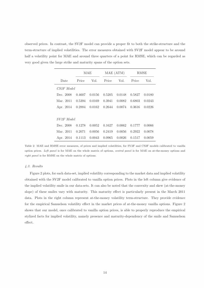
observed prices. In contrast, the SV2F model can provide a proper fit to both the strike-structure and the
term-structure of implied volatilities. The error measures obtained with SV2F model appear to be around
half a volatility point for MAE and around three quarters of a point for RMSE, which can be regarded as
very good given the large strike and maturity spans of the option sets.
MAE MAE (ATM) RMSE
Date Price Vol. Price Vol. Price Vol.
CS2F Model
Dec. 2008 0.4607 0.0156 0.5205 0.0148 0.5827 0.0180
Mar. 2011 0.5394 0.0169 0.3941 0.0082 0.6803 0.0243
Apr. 2014 0.2884 0.0162 0.2644 0.0074 0.3616 0.0226
SV2F Model
Dec. 2008 0.1278 0.0052 0.1627 0.0062 0.1777 0.0066
Mar. 2011 0.2071 0.0056 0.2419 0.0056 0.2922 0.0078
Apr. 2014 0.1113 0.0043 0.0965 0.0026 0.1517 0.0059
Table 2: MAE and RMSE error measures, of prices and implied volatilities, for SV2F and CS2F models calibrated to vanilla
option prices. Left panel is for MAE on the whole matrix of options, central panel is for MAE on at-the-money options and
right panel is for RMSE on the whole matrix of options.
4.3. Results
Figure 2 plots, for each data-set, implied volatility corresponding to the market data and implied volatility
obtained with the SV2F model calibrated to vanilla option prices. Plots in the left column give evidence of
the implied volatility smile in our data-sets. It can also be noted that the convexity and skew (at-the-money
slope) of these smiles vary with maturity. This maturity effect is particularly present in the March 2011
data. Plots in the right column represent at-the-money volatility term-structure. They provide evidence
for the empirical Samuelson volatility effect in the market prices of at-the-money vanilla options. Figure 2
shows that our model, once calibrated to vanilla option prices, is able to properly reproduce the empirical
stylized facts for implied volatility, namely presence and maturity-dependency of the smile and Samuelson
effect.
14

30 40 50 60 70 80 90 100 1100
0.1
0.2
0.3
0.4
0.5
0.6
0.7
0.8
0.9
1
K
WTI 2008
0 0.5 1 1.5 2 2.5 3 3.5 4 4.5 50
0.1
0.2
0.3
0.4
0.5
0.6
0.7
0.8
0.9
1
T
WTI 2008
60 80 100 120 140 160 1800.1
0.2
0.3
0.4
0.5
0.6
K
WTI 2011
0 0.5 1 1.5 2 2.5 3 3.5 4 4.5 50.1
0.2
0.3
0.4
0.5
0.6
T
WTI 2011
40 60 80 100 120 140 1600.05
0.1
0.15
0.2
0.25
0.3
0.35
0.4
0.45
K
WTI 2014
0 0.5 1 1.5 2 2.5 3 3.5 4 4.5 50.05
0.1
0.15
0.2
0.25
0.3
0.35
0.4
0.45
T
WTI 2014
Figure 2: Implied volatilities corresponding to market quotes and obtained with SV2F model calibrated to vanilla options. Left
column: implied volatility smiles. Right column: at-the-money implied volatility term-structure.
Figure 3 plots, for the data-sets of December 2008 and March 2011, measures of concordance and de-
pendence between two futures prices produced by the calibrated SV2F model. This figure represents a type
of dependence term-structure that is of interest for WTI futures market participants. It corresponds to the
case where the time horizon and the first futures expiry are both held constant, while the difference between
futures expiries varies. We observe that, as the difference between expiries increases, the pair of futures
becomes less dependent which is in line with the intuition one can have a priori. We call this phenomenon
the Samuelson correlation effect. This phenomenon is a desirable feature for a model to be used by a price
maker quoting and trading a range of products written on WTI. The presented empirical applications show
it is properly reproduced by the proposed model.
Figure 4 plots, for the data-sets of December 2008 and March 2011, measures of concordance and depen-
15

dence between two futures prices produced by the calibrated SV2F model. It corresponds to the case where
the time horizon varies while the difference between futures expiries is held constant. For the December 2008
case, the level of dependence between the futures is little affected by the time-horizon. For the March 2011
case, as the time-horizon increases, the pairs of futures with 6-month difference between their maturities
become more dependent. Here the intuition does not lead to a particular structure that is desirable, namely
increasing or decreasing as the time horizon varies.
0.2 0.3 0.4 0.5 0.6 0.7 0.8 0.9 10.1
0.2
0.3
0.4
0.5
0.6
0.7
0.8
0.9
1
T2-T
1
0.2 0.3 0.4 0.5 0.6 0.7 0.8 0.9 10
0.1
0.2
0.3
0.4
0.5
0.6
0.7
0.8
0.9
T2-T
1
Figure 3: Term-structure of concordance and dependence measures between F (T, T1) and F (T, T2) produced by the SV2F
model calibrated market data. Left panel corresponds to December 2008 data and right panel corresponds to March 2011 data.
Time horizon T and first futures expiry T1 are fixed at 3 months, T2−T1 ranges from 3 months to 1 year. Dependence measures
are τK and S (respectively, green and blue lines). Concordance measures are σSW and ΦH (respectively, red and black lines).
0.2 0.3 0.4 0.5 0.6 0.7 0.8 0.9 10
0.1
0.2
0.3
0.4
0.5
0.6
0.7
0.8
0.9
1
T
0.2 0.3 0.4 0.5 0.6 0.7 0.8 0.9 10
0.1
0.2
0.3
0.4
0.5
0.6
0.7
0.8
0.9
1
T
Figure 4: Term-structure of concordance and dependence measures between F (T, T1) and F (T, T2) produced by the SV2F
model calibrated market data. Left panel corresponds to December 2008 data and right panel corresponds to March 2011 data.
Time horizon T and first futures expiry T1 range from 3 months to 1 year. T2 − T1 is held fixed at 6 months. Dependence
measures are τK and S (respectively, green and blue lines). Concordance measures are σSW and ΦH (respectively, red and
black lines).
Figure 5 plots the implied correlation strike and maturity structures from spread option prices obtained
with the SV2F model calibrated to the data-sets of December 2008 and March 2011. The considered spread
options have fixed maturity and first futures expiry, while the difference between the two underlying futures
expiries varies. For each pair of underlying futures, the five strikes correspond to a set of shifts applied to the
16

at-the-money spread F (0, T1) − F (0, T2). These shifts are −10,−5,−2.5, 0,+2.5,+5 and +10. We observe
that the obtained term-structures are decreasing. This observation is in line with the intuition and with
what is observed in Figure 3, i.e. with the Samuelson correlation effect. For the March 2011 case, the model
produces a non-constant strike structure of implied correlation. We observe that for larger strikes (out-of-
the-money call spread options) implied correlations are lower than at-the-money. Lower implied correlations
in turn correspond to higher option prices. For the December 2008 case, the model produces a rather flat
strike structure of implied correlation. Hence, in this case, the prices produced by the model are close to
prices that could have been produced using Gaussian copulas for the dependence between futures prices.
Figure 6 plots the implied correlation strike and maturity structures from spread option prices obtained
with the SV2F model calibrated to the data-sets of December 2008 and March 2011. The considered spread
options have maturity and first futures expiry that vary, while the difference between the two underlying
futures expiries is held constant. For each pair of underlying futures, the five strikes correspond to a set of
shifts applied to the at-the-money spread F (0, T1)−F (0, T2). These shifts are the same as for Figure 5. We
observe that the obtained term-structures are decreasing. The obtained term-structure for December 2008
is rather flat which is consistent with the term-structure of concordance and dependence presented in Figure
4. For the March 2011 case, the implied correlation term-structure is increasing which is again consistent
with concordance and dependence measures in Figure 4. For the March 2011 case, the model produces a
non-constant strike structure of implied correlation. For the December 2008 case, the model produces a
rather flat strike structure of implied correlation. These strike structures are similar to those found in Figure
5 and the same comments apply.
17

-10 -5 0 5 10 15 200.5
0.6
0.7
0.8
0.9
1
K
WTI 2008
0.2 0.3 0.4 0.5 0.6 0.7 0.8 0.9 10.5
0.6
0.7
0.8
0.9
1
T2-T
1
WTI 2008
-10 -5 0 5 100.5
0.6
0.7
0.8
0.9
1
K
WTI 2011
0.2 0.3 0.4 0.5 0.6 0.7 0.8 0.9 10.5
0.6
0.7
0.8
0.9
1
T2-T
1
WTI 2011
Figure 5: Implied correlations from spread option prices obtained with the SV2F model calibrated to market data of December
2008 and March 2011. The considered spread options have a maturity T and first underlying futures expiry T1 fixed at 3
months. T2 − T1, the difference between the underlying futures expiries, ranges from 3 months to 1 year. Left column: implied
correlation smiles. Right column: at-the-money implied correlation term-structure.
18

-10 -5 0 5 10 150.5
0.6
0.7
0.8
0.9
1
K
WTI 2008
0.2 0.3 0.4 0.5 0.6 0.7 0.8 0.9 10.5
0.6
0.7
0.8
0.9
1
T
WTI 2008
-10 -5 0 5 100.5
0.6
0.7
0.8
0.9
1
K
WTI 2011
0.2 0.3 0.4 0.5 0.6 0.7 0.8 0.9 10.5
0.6
0.7
0.8
0.9
1
T
WTI 2011
Figure 6: Implied correlations from spread option prices obtained with the SV2F model calibrated to market data of December
2008 and March 2011. The considered spread options have a maturity T and first underlying futures expiry T1 varying from
3 months to 1 year. T2 − T1, the difference between the underlying futures expiries, is held fixed at 6 months. Left column:
implied correlation smiles. Right column: at-the-money implied correlation term-structure.
5. Conclusion
We propose a multi-factor stochastic volatility model for commodity futures contracts. In order to
capture the Samuelson effect displayed by commodity futures contracts, we add expiry-dependent exponential
damping factors to their volatility coefficients. The pricing of single underlying European options on futures
contracts is straightforward and can incorporate the volatility smile or skew observed in the market. We
calculate the joint characteristic function of two futures contracts in the model and use the one-dimensional
Fourier inversion method of Caldana and Fusai (2013) to price calendar spread options. Furthermore, we
analyze the term-structure of dependence between pairs of futures in the model. We do this by showing
how to obtain the copula and copula density functions directly from the joint characteristic function. When
calibrated to vanilla options, the model is found to be able to produce stylized facts such as Samuelson effect
and implied volatility smile as well as a decreasing term-structure of dependence and implied correlation
smile for spread options.
19

6. Proofs
Proof. (Proposition 1)
We have
φ(u) = φ(u;T, T1, T2) = E
[
exp
(
i
2∑
k=1
ukXk(T )
)]
= E
exp
i
2∑
k=1
uk
n∑
j=1
∫ T
0
e−λj(Tk−t)√
vj(t)dBj(t)−1
2
n∑
j=1
∫ T
0
e−2λj(Tk−t)vj(t)dt
=
n∏
j=1
Ej(u, T ),
where Ej is a function of u and T given by
Ej(u, T ) = E
[
exp
(
i
2∑
k=1
uk
{
∫ T
0
e−λj(Tk−t)√
vj(t)dBj(t)−1
2
∫ T
0
e−2λj(Tk−t)vj(t)dt
})]
that otherwise depends only on the j-th model parameters λj , κj , θj , σj , vj,0, ρj .
We now calculate the function Ej . Since we are considering a fixed value of j, we drop this subscript
in the following calculations. We also write B for Bn+j , the Brownian motion driving the j-th variance
process. Then we can decompose B = Bj , whose correlation with B = Bn+j is given in equation (3) by
〈Bj , Bn+j〉 = ρjdt = ρdt, as B = ρB +√
1− ρ2B, where B is uncorrelated with B. Define the functions
f1, f2 and q given by
f1(u, t) =2∑
k=1
uke−λ(Tk−t), f2(u, t) =
2∑
k=1
uke−2λ(Tk−t),
q(u, t) = iρκ− λ
σf1(u, t)−
1
2(1− ρ2)f2
1 (u, t)−1
2if2(u, t).
For simplicity, we write f1(t) for f1(u, t), f2(t) for f2(u, t) and q(t) for q(u, t) in the following.
We first need an auxiliary result in order to calculate the characteristic function.
Lemma 6.
σ
∫ T
0
f1(t)√
v(t)dB(t) =
[
f1(t)
{
v(t)− κθ
λ
}]T
0
+ (κ− λ)
∫ T
0
f1(t)v(t)dt. (29)
Proof. (Lemma 6)
Multiplying equation (2) by f1(t) and then integrating from 0 to T gives
∫ T
0
f1(t)dv(t) =
∫ T
0
f1(t)κ(θ − v(t))dt+ σ
∫ T
0
f1(t)√
v(t)dB(t). (30)
Using Ito-integration by parts (see Øksendal (2003)), we also have
∫ T
0
f1(t)dv(t) = [f1(t)v(t)]T0 −
∫ T
0
v(t)df1(t) = [f1(t)v(t)]T0 − λ
∫ T
0
f1(t)v(t)dt. (31)
20

Equating the right hand sides of equations (30) and (31) gives
σ
∫ T
0
f1(t)√
v(t)dB(t) = [f1(t)v(t)]T0 − λ
∫ T
0
f1(t)v(t)dt−∫ T
0
f1(t)κ(θ − v(t))dt
= [f1(t)v(t)]T0 − κθ
∫ T
0
f1(t)dt+ (κ− λ)
∫ T
0
f1(t)v(t)dt
=
[
f1(t)
{
v(t)− κθ
λ
}]T
0
+ (κ− λ)
∫ T
0
f1(t)v(t)dt,
which proves the lemma.
We now calculate E(u, T ).
E(u, T ) =
[
exp
(
i
2∑
k=1
uk
{
∫ T
0
e−λ(Tk−t)√
v(t)dB(t)− 1
2
∫ T
0
e−2λ(Tk−t)v(t)dt
})]
= E
[
exp
(
i
∫ T
0
f1(t)√
v(t)dB(t)− 1
2i
∫ T
0
f2(t)v(t)dt
)]
= E
[
exp
(
iρ
∫ T
0
f1(t)√
v(t)dB(t) + i√
1− ρ2∫ T
0
f1(t)√
v(t)dB(t)− 1
2i
∫ T
0
f2(t)v(t)dt
)]
= E
[
exp
(
iρ
∫ T
0
f1(t)√
v(t)dB(t)− 1
2(1− ρ2)
∫ T
0
(f1(t))2v(t)dt− 1
2i
∫ T
0
f2(t)v(t)dt
)]
= E
[
exp(
iρ
σ
[
f1(t)
{
v(t)− κθ
λ
}]T
0
+ iρκ− λ
σ
∫ T
0
f1(t)v(t)dt
− 1
2(1− ρ2)
∫ T
0
(f1(t))2v(t)dt− 1
2i
∫ T
0
f2(t)v(t)dt)]
= exp
(
iρ
σ
{
κθ
λ(f1(0)− f1(T ))− f1(0)v(0)
})
· E[
exp
(
iρ
σf1(T )v(T ) +
∫ T
0
q(t)v(t)dt
)]
.
The expectation in the last line can be computed using the Feynman-Kac theorem (see Øksendal (2003)).
Define the function h given by
h(t, v) = E
[
exp
(
iρ
σf1(T )v(T ) +
∫ T
t
q(s)v(s)ds
)]
.
Then h satisfies the PDE
∂h
∂t(t, v) + κ(θ − v(t))
∂h
∂v(t, v) +
1
2σ2v(t)
∂2h
∂v2(t, v) + q(t)v(t)h(t, v) = 0, (32)
with terminal condition h(T, v) = exp(
i ρσf1(T )v(T )
)
. We know from Duffie et al. (2000) that h has affine
form
h(t, v) = exp (A(t, T )v(t) +B(t, T )) , (33)
with A(T, T ) = i ρσf1(T ), B(T, T ) = 0. Putting (33) in (32) gives
Bt +Atv + κ(θ − v)A+1
2σ2vA2 + qv = 0,
21

and collecting the terms with and without v leads to the two ODEs
At − κA+1
2σ2A2 + q = 0, (34)
Bt + κθA = 0. (35)
This completes the proof of the proposition.
Proof. (Proposition 3)
We calculate the joint characteristic function in the Clewlow and Strickland (1999a) model as follows.
φ(u) = φ(u;T, T1, T2)
= E
[
exp
(
i
2∑
k=1
ukXk(T )
)]
= E
exp
i
2∑
k=1
uk
n∑
j=1
∫ T
0
e−λj(Tk−t)σjdBj(t)−1
2
n∑
j=1
∫ T
0
e−2λj(Tk−t)σ2jdt
=
n∏
j=1
E
[
exp
(
i
2∑
k=1
uk
{
∫ T
0
e−λj(Tk−t)σjdBj(t)−1
2
∫ T
0
e−2λj(Tk−t)σ2jdt
})]
=
n∏
j=1
exp
(
i
2∑
k=1
uk
{
−1
2
∫ T
0
e−2λj(Tk−t)σ2jdt
})
E
[
exp
(
i
2∑
k=1
uk
{
∫ T
0
e−λj(Tk−t)σjdBj(t)
})]
=n∏
j=1
exp
i
2∑
k=1
uk
[
−σ2j
4λj
e−2λj(Tk−t)
]T
0
exp
−
σ2j
4λj
(
2∑
k=1
uke−λj(Tk−t)
)2
T
0
=n∏
j=1
exp
(
−σ2j
4λj
(e2λjT − 1){
i(u1e−2λjT1 + u2e
−2λjT2) + (u1e−λjT1 + u2e
−λjT2)2}
)
.
This completes the proof of the proposition.
Proof. (Lemma 4)
The proof to obtain this expression is the same, mutatis mutandis, as the proof in the univariate case
provided in Le Courtois and Walter (2015). For ease of reading, we drop the explicit dependencies on T, T1
and T2. Let a1 > 0 and a2 > 0 be fixed and h be the function defined by
h(x1, x2) = e−(a1x1+a2x2)G(x1, x2) = e−(a1x1+a2x2)
∫ x2
−∞
∫ x1
−∞g(s1, s2)ds1ds2.
Now let Λ be the two-dimensional Fourier Transform of h. We have
Λ(u1, u2) =
∫ +∞
−∞
∫ +∞
−∞ei(u1x1+u2x2)h(x1, x2)dx1dx2
=
∫ +∞
−∞
∫ +∞
−∞ei(u1x1+u2x2)
(
e−(a1x1+a2x2)
∫ x2
−∞
∫ x1
−∞g(s1, s2)ds1ds2
)
dx1dx2
=
∫ +∞
−∞
∫ +∞
−∞
∫ x2
−∞
∫ x1
−∞ei(u1x1+u2x2)e−(a1x1+a2x2)g(s1, s2)ds1ds2dx1dx2.
22

Noting that −∞ < s1 < x1 < +∞ and −∞ < s2 < x2 < +∞, the expression of Λ becomes
Λ(u1, u2) =
∫ +∞
−∞
∫ +∞
−∞
∫ +∞
s2
∫ +∞
s1
ei(u1x1+u2x2)e−(a1x1+a2x2)g(s1, s2)dx1dx2ds1ds2
=
∫ +∞
−∞
∫ +∞
−∞g(s1, s2)
(∫ +∞
s2
∫ +∞
s1
ei(u1x1+u2x2)e−(a1x1+a2x2)dx1dx2
)
ds1ds2.
The double integral between parentheses can be computed as
∫ +∞
s2
∫ +∞
s1
ei(u1x1+u2x2)e−(a1x1+a2x2)dx1dx2 =
[
e−(a1−iu1)x1
−(a1 − iu1)
]+∞
s1
[
e−(a2−iu2)x2
−(a2 − iu2)
]+∞
s2
.
Note that∣
∣e−(a1−iu1)x1
∣
∣ −→ 0 when x1 goes to +∞ and∣
∣e−(a2−iu2)x2
∣
∣ −→ 0 when x2 goes to +∞, so that
we obtain
Λ(u1, u2) =
∫ +∞
−∞
∫ +∞
−∞g(s1, s2)
(
−e−(a1−iu1)s1
−(a1 − iu1)
)(
−e−(a2−iu2)s2
−(a2 − iu2)
)
ds1ds2
=1
(a1 − iu1)(a2 − iu2)
∫ +∞
−∞
∫ +∞
−∞g(s1, s2)e
i((u1+ia1)s1+(u2+ia2)s2)ds1ds2
=φ(u1 + ia1, u2 + ia2)
(a1 − iu1)(a2 − iu2).
The function h can be written as the two-dimensional inverse Fourier Transform of Λ:
h(x1, x2) =1
4π2
∫ +∞
−∞
∫ +∞
−∞e−i(u1x1+u2x2)
φ(u1 + ia1, u2 + ia2)
(a1 − iu1)(a2 − iu2)du1du2,
and G is then easily obtained as
G(x1, x2) =ea1x1+a2x2
4π2
∫ +∞
−∞
∫ +∞
−∞e−i(u1x1+u2x2)
φ(u1 + ia1, u2 + ia2)
(a1 − iu1)(a2 − iu2)du1du2,
which concludes the proof.
Proof. (Proposition 5)
Sklar’s Theorem allows one to write the copula function of a pair of random variables from its joint
distribution function as, for (v1, v2) ∈ [0, 1]2,
C(v1, v2, T ) = G(
G−11 (v1, T ), G
−12 (v2, T ), T
)
.
The expression for the copula function in Proposition 5 follows by using Lemma 4, which expresses the
joint distribution function in terms of the joint characteristic function φ. Assuming C(., T ) is absolutely
continuous, we can write its copula density, for (v1, v2) ∈ [0, 1]2, as
c(v1, v2, T ) =g(G−1
1 (v1, T ), G−12 (v2, T ), T )
g1(G−11 (v1, T ), T )g2(G
−12 (v2, T ), T )
.
Again, the expression for the copula density in Proposition 5 follows by using expressions (22), (23) and (24)
that express the joint and marginal densities of (X1(T ), X2(T )) in terms of the joint characteristic function
φ.
23

Acknowledgements
We thank Iain Clark, Jean-Baptiste Gheeraert, Cassio Neri, Damien Pons, Matthias Scherer, and seminar
participants at the 53rd Meeting of the Euro Working Group on Commodities and Financial Modelling,
the International Ruhr Energy Conference 2015, and the World Finance Conference 2015 for helpful and
stimulating comments, discussions and suggestions. All remaining errors are our own.
Appendix A. Kummer’s functions
The functions M and U are the confluent hypergeometric functions. The function M is also known as
1F1, and the function U as Tricomi’s function. Given, a, b, z ∈ C, Kummer’s equation is
z∂2w
∂z2+ (b− z)
∂w
∂z− aw = 0. (A.1)
A way to obtain M(a, b, z) is by means of the series expansion
M(a, b, z) = 1 +
∞∑
n=1
zn∏n
j=1 (a+ j − 1)
n!∏n
j=1 (b+ j − 1). (A.2)
And U(a, b, z) is obtained from M as
U(a, b, z) =π
sin (πb)
(
M(a, b, z)
Γ(1 + a− b)Γ(b)− z1−bM(1 + a− b, 2− b, z)
Γ(a)Γ(2− b)
)
, (A.3)
where Γ denotes the Gamma function extended to the complex plane. These results and additional properties
of Kummer’s functions (e.g. integral representations) can be found in Chap. 13 of Abramovitz and Stegun
(1972). A detailed analysis of how to implement Kummer’s functions is given by Pearson (2009). A suitable
way to implement the complex Gamma function is the Lanczos (1964) approximation.
Appendix B. The Caldana and Fusai method for pricing calendar spread options.
Let ΦT (u) = Φ(u) be the joint characteristic function of the logarithms lnF (T, T1), lnF (T, T2) of two
futures prices as given in the main manuscript. Following Caldana and Fusai (2013), the price of the calendar
spread option call with maturity T and strike K is given in terms of a Fourier inversion formula as
CSC(0,K, T, T1, T2) =
(
e−δk−rT
π
∫ +∞
0
e−iγkΨT (γ; δ, α)dγ
)+
, (B.1)
where
ΨT (γ; δ, α) =ei(γ−iδ) ln(ΦT (0,−iα))
i(γ − iδ)
· [ΦT ((γ − iδ)− i,−α(γ − iδ))− ΦT (γ − iδ,−α(γ − iδ)− i)−KΦT (γ − iδ,−α(γ − iδ))]
and
α =F (0, T2)
F (0, T2) +K, k = ln(F (0, T2) +K).
The parameter δ controls an exponential decay term as in Carr and Madan (1999).
24

Appendix C. FFT Methods
An FFT algorithm allows the efficient computation of Discrete Fourier Transforms (DFT) of vectors and
matrices. Here we will discuss Matlab and Numerical Recipes in C++ functions but other numerical analysis
tools, such as Mathematica and R, are of course also suitable.
Matlab functions:
In one dimension, the Matlab routines fft and ifft work with vectors and implement the following
sums, respectively:
x(k) =N∑
n=1
X(n)W(n−1)(k−1)N X(n) =
1
N
N∑
k=1
x(k)W−(n−1)(k−1)N (C.1)
where WN = e−2πiN is a Nth root of unity.
In two dimensions, the Matlab routines fft2 and ifft2 work with matrices and implement the following
sums, respectively:
x(k1, k2) =N∑
n1=1
N∑
n2=1
X(n1, n2)W[(n1−1)(k1−1)+(n2−1)(k2−1)]N (C.2)
X(n1, n2) =1
N2
N∑
k1=1
N∑
k2=1
x(k1, k2)W−[(n1−1)(k1−1)+(n2−1)(k2−1)]N (C.3)
where WN = e−2πiN is an Nth root of unity.
Numerical Recipes in C++ functions:
In one dimension, the function four1 works with vectors and implements the following sums when
choosing isign = 1 and −1, respectively:
H(n) =
N−1∑
k=0
h(k)WnkN h(k) =
N−1∑
n=0
H(n)W−nkN (C.4)
where WN = e2πiN is a Nth root of unity.
In two dimensions, the function fourn works with matrices and implements the following sums when
choosing isign = 1 and −1, respectively:
H(n1, n2) =
N−1∑
k1=0
N−1∑
k2=0
h(k1, k2)Wn1k1+n2k2
N (C.5)
h(k1, k2) =N−1∑
n1=0
N−1∑
n2=0
H(n1, n2)W−(n1k1+n2k2)N (C.6)
where WN = e2πiN is an Nth root of unity (note that WN is not the same as in Matlab).
25

Appendix D. Marginal CDF and PDF
We are first interested in the marginal CDF and PDF of X1(T ).
Let N be the chosen number of points on the grid (e.g. N = 512) and let xk1=(
k1 − N2
)
h with
k1 = 0, . . . , N −1. h is the chosen distance between points in the initial domain. The grid in x is centered on
xN2
= 0. In the transformed domain we work with ω = u2π that represents angular frequency (u represents
frequency or inverse wavelength). N is also the chosen number of points on the grid in ω with ωn1=
(
n1 − N2
)
s with n1 = 0, . . . , N − 1. s = 1hN
is the distance between points in the transformed domain. The
grid in the transformed domain is centered on ωN2
= 0.
At a point xk1, choosing the rectangle rule on the grid in ω, the PDF g1 is approximated as
g1(xk1, T ) =
∫ +∞
−∞e−i2πω(k1−N
2 )hφ(2πω, 0, T )dω ≈ s
N−1∑
n1=0
e−i2π(n1−N2 )(k1−N
2 )shφ(2πωn1, 0, T ) (D.1)
≈ s(−1)k1−N2
N−1∑
n1=0
(−1)n1φ(2πωn1, 0, T )en1k1
−i2πN (D.2)
where the powers of −1 appear when rearranging terms and noting that eiqπ = (−1)q for q ∈ Z. When N is
a power of 2, the obtained expression is suitable for FFT algorithms at hand. For x0, . . . , xN−1, the sums
can be computed by calling just once the FFT function on the vector
[(−1)nφ(2πωn1), n1 = 0, . . . , N − 1] .
In Matlab it corresponds to the fft routine and in Numerical Recipes to the function four1 with isign= −1.
Other approximations can be obtained using different numerical integration rules (e.g. trapezoidal, Simpson).
With the same grids and notations, at a point xk1, the CDF G1 is written, with a > 0,
G1(xk1, T ) =
1
2− 1
2π
∫ +∞
−∞e−iuxk1
φ(u)
iudu =
eaxk1
2π
∫ +∞
−∞e−iuxk1
φ(u+ ia, 0, T )
a− iudu. (D.3)
A proper choice for the value of a (e.g. a = 3) will permit a smoothing of the singularity at u = 0 of the
integrand in the initial CDF inversion result. At a point xk1, choosing the rectangle rule on the grid in ω,
the CDF G1 can now be approximated as
G1(xk1, T ) ≈ eaxk1 s
N−1∑
n1=0
φ(2πωn1+ ia, 0, T )
a− i2πωn1
e−i2π(n1−N2 )(k1−N
2 )sh, (D.4)
≈ eaxk1 s(−1)k1−N2
N−1∑
n1=0
(−1)n1φ(2πωn1
+ ia, 0, T )
a− i2πωn1
en1k−i2πN . (D.5)
The powers of −1 appear once again for the reason already mentioned. With N a power of 2, the obtained
expression is suitable for FFT algorithms and the needed sums on the x-grid are computed by calling just
once the FFT function on the vector[
(−1)n1φ(2πωn1
+ ia)
a− i2πωn1
, n1 = 0, . . . , N − 1
]
.
26

In Matlab it corresponds to the fft routine and in Numerical Recipes to the function four1 with isign= −1.
Once G1 has been implemented, it is rather easy to implement the inverse CDF G−11 either with a
numerical root search or by doing a reverse interpolation on the pair of vectors
([x0, . . . , xN−1] , [G1(x0), . . . , G1(xN−1)]) .
Appendix E. Joint CDF and PDF
Let N be again the chosen number of points on the one-dimensional grids in x1 and x2 (e.g. N = 512)
and let xk1=(
k1 − N2
)
h and xk2=(
k2 − N2
)
h with k1, k2 = 0, . . . , N − 1. h is the chosen distance between
points in the initial domain. The grid is centered on(
xN2
, xN2
)
= (0, 0). In the transformed domain we
work with υ = u1
2π and ω = u2
2π . N is also the chosen number of points on the one-dimensional grids in υ and
ω with υn1=(
n1 − N2
)
s and ωn2=(
n2 − N2
)
s with n1, n2 = 0, . . . , N − 1. s = 1hN
is the distance between
points in the transformed domain. The grid in the transformed domain is centered on(
υN2
, ωN2
)
= (0, 0).
At a point (xk1, xk2
), choosing the two-dimensional rectangle rule on the grid in (υ, ω), the joint PDF g is
approximated as
g(xk1, xk2
, T ) =
∫ +∞
−∞
∫ +∞
−∞e−i2π(υxk1
+ωxk2)φ(2πυ, 2πω, T )dυdω, (E.1)
≈ s2N−1∑
n1=0
N−1∑
n2=0
φ(2πυn1, 2πωn2
, T )e−i2π[(n1−N2 )(k1−N
2 )+(n2−N2 )(k2−N
2 )]sh, (E.2)
≈ s2(−1)k1+k2−N
N−1∑
n1=0
N−1∑
n2=0
(−1)n1+n2φ(2πυn1, 2πωn2
, T )e(n1k1+n2k2)−i2πN . (E.3)
With N a power of 2, the obtained expression is suitable for FFT algorithms in 2D and the needed sums
on the (x1, x2)-grid are computed by calling just once the FFT function on the matrix
[(−1)n1,n2φ(2πυn1, 2πωn2
, T ), n1, n2 = 0, . . . , N − 1]
In Matlab it corresponds to the fft2 routine and in Numerical Recipes to the function fourn with isign=
−1.
With the same grids and notations, at a point (xk1, xk2
), the joint CDF G can be written, with a1, a2 > 0,
G(xk1, xk2
, T ) =ea1xk1
+a2xk2
4π2
∫ +∞
−∞
∫ +∞
−∞e−i(u1xk1
+u2xk2)φ(u1 + ia1, u2 + ia2, T )
(a1 − iu1)(a2 − iu2)du1du2 (E.4)
Here again, a proper choice for the value of a1 and a2 (e.g. a1 = a2 = 3) will permit a smoothing of the
singularity of the integrand on the axis u1 = 0 and u2 = 0 in the initial joint CDF inversion result.
27

At a point (xk1, xk2
), choosing the two-dimensional rectangle rule on the grid in (υ, ω), the joint CDF G
is approximated as
G(xk1, xk2
, T ) = ea1xk1+a2xk2
∫ +∞
−∞
∫ +∞
−∞e−i2π(υxk1
+ωxk2)φ(2πυ + ia1, 2πω + ia2, T )
(a1 − i2πυ)(a2 − i2πω)dυdω, (E.5)
≈ ea1xk1+a2xk2 s2
N−1∑
n1=0
N−1∑
n2=0
φ(2πυn1+ ia1, 2πωn2
+ ia2, T )
(a1 − i2πυn1)(a2 − i2πωn2
)e−i2π[(n1−N
2 )(k1−N2 )+(n2−N
2 )(k2−N2 )]sh, (E.6)
≈ ea1xk1+a2xk2 s2(−1)k1+k2−N
N−1∑
n1=0
N−1∑
n2=0
(−1)n1+n2φ(2πυn1
+ ia1, 2πωn2+ ia2, T )
(a1 − i2πυn1)(a2 − i2πωn2
)e(n1k1+n2k2)
−i2πN . (E.7)
With N a power of 2, the obtained expression is suitable for FFT algorithms in 2D and the needed sums
on the (x1, x2)-grid are computed by calling just once the FFT function on the matrix
[
(−1)n1,n2φ(2πυn1
+ ia1, 2πωn2+ ia2, T )
(a1 − i2πυn1)(a2 − i2πωn2
), n1, n2 = 0, . . . , N − 1
]
In Matlab it corresponds to the fft2 routine and in Numerical Recipes to the function fourn with isign=
−1.
28

References
Abramovitz, M., Stegun, I. A., 1972. Handbook of mathematical functions, tenth printing Edition. Applied
Mathematics Series 55. National Bureau of Standards.
Bakshi, G., Cao, C., Chen, Z., December 1997. Empirical performance of alternative option pricing models.
Journal of Finance 52 (5), 2003–2049.
Bakshi, G., Madan, D., 2000. Spanning and derivative-security valuation. Journal of Financial Economics
55 (2), 205–238.
Barone-Adesi, G., Whaley, R. E., June 1987. Efficient analytic approximation of American option values.
Journal of Finance 42 (2), 301–320.
Bessembinder, H., Coughenour, J. F., Seguin, P. J., Smoller, M. M., Winter 1996. Is there a term structure
of futures volatilities? Reevaluating the Samuelson hypothesis. Journal of Derivatives 4 (2), 45–58.
Bjerksund, P., Stensland, G., 2011. Closed form spread option valuation. Quantitative Finance iFirst, 1–10.
Black, F., March 1976. The pricing of commodity contracts. Journal of Financial Economics 3 (1-2), 167–179.
Brooks, R., Winter 2012. Samuelson hypothesis and carry arbitrage. Journal of Derivatives 20 (2), 37–65.
Caldana, R., Fusai, G., December 2013. A general closed-form spread option pricing formula. Journal of
Banking and Finance 37 (12), 4893–4906.
Carmona, R., Durrleman, V., 2003. Pricing and hedging spread options. SIAM Review 45 (4), 627–685.
Carr, P., Madan, D. B., 1999. Option valuation using the Fast Fourier Transform. Journal of Computational
Finance 2 (4), 61–73.
Chockalingam, A., Muthuraman, K., July–August 2011. American options under stochastic volatility. Oper-
ations Research 59 (4), 793–809.
Christoffersen, P., Heston, S., Jacobs, K., December 2009. The shape and term structure of the index option
smirk: Why multifactor stochastic volatility models work so well. Management Science 55 (12), 1914–1932.
Clark, I. J., 2014. Commodity Option Pricing: A Practitioner’s Guide. Wiley Finance. Wiley.
Clewlow, L., Strickland, C., August 1999a. A multi-factor model for energy derivatives, working Paper, 20
pages.
Clewlow, L., Strickland, C., April 1999b. Valuing energy options in a one factor model fitted to forward
prices, working Paper, 30 pages.
29

Cox, J. C., Ingersoll, J. E., Ross, S. A., 1985. A theory of the term structure of interest rates. Econometrica
53, 385–408.
Duffie, D., Pan, J., Singleton, K., November 2000. Transform analysis and asset pricing for affine jump-
diffusions. Econometrica 68 (6), 1343–1376.
Heston, S., 1993. A closed-form solution for options with stochastic volatility with applications to bond and
currency options. Review of Financial Studies 6 (2), 327–343.
Hull, J., White, A., June 1987. The pricing of options on assets with stochastic volatilities. Journal of Finance
42 (2), 281–100.
Hurd, T. R., Zhou, Z., 2010. A Fourier transform method for spread option pricing. SIAM Journal on
Financial Mathematics 1 (1), 142–157.
Kirk, E., 1995. Correlations in the energy markets. Managing Energy Price Risk, 71–78.
Lanczos, C., 1964. A precision approximation of the Gamma function. SIAM Journal on Numerical Analysis
series B 1, 86–96.
Le Courtois, O., Walter, C., 2015. The computation of risk budgets under the Levy process assumption.
Finance 35 (2).
Longstaff, F. A., Schwartz, E. S., 2001. Valuing American options by simulation: A simple least-squares
approach. Review of Financial Studies 14 (1), 113–147.
Mai, J.-F., Scherer, M., 2012. Simulating Copulas: Stochastic Models, Sampling Algorithms, and Applica-
tions. Vol. 4 of Series in Quantitative Finance. Imperial College Press.
Margrabe, W., March 1978. The value of an option to exchange one asset for another. Journal of Finance
33 (1), 177–186.
Nelsen, R. B., 2006. An Introduction to Copulas, 2nd Edition. Springer Series in Statistics. Springer.
Øksendal, B., 2003. Stochastic Differential Equations: An Introduction with Applications, sixth Edition.
Universitext. Springer.
Pearson, J., September 2009. Computation of hypergeometric functions. Master’s thesis, University of Ox-
ford.
Samuelson, P. A., Spring 1965. Proof that properly anticipated prices fluctuate randomly. Industrial Man-
agement Review 6 (2), 41–49.
Schoebel, R., Zhu, J., 1999. Stochastic volatility with an Ornstein-Uhlenbeck process: An extension. Euro-
pean Finance Review 3, 23–46.
30

Scott, L. O., December 1987. Option pricing when the variance changes randomly: Theory, estimation, and
an application. Journal of Financial and Quantitative Analysis 22 (4), 419–438.
Scott, L. O., October 1997. Pricing stock options in a jump-diffusion model with stochastic volatility and
interest rates: Applications of Fourier inversion methods. Mathematical Finance 7 (4), 413–424.
Trolle, A. B., Schwartz, E. S., 2009. Unspanned stochastic volatility and the pricing of commodity derivatives.
Review of Financial Studies 22 (11), 4423–4461.
Venkatramanan, A., Alexander, C., November 2011. Closed-form approximations for spread options. Applied
Mathematical Finance 18 (5), 447–472.
31


