FLEXURAL BEHAVIOR OF
REINFORCED AND PRESTRESSED CONCRETE BEAMS
USING FINITE ELEMENT ANALYSIS
by
Anthony J. Wolanski, B.S.
A Thesis submitted to the Faculty of the Graduate School,
Marquette University, in Partial Fulfillment of
the Requirements for the Degree of
Master of Science
Milwaukee, Wisconsin May, 2004
PREFACE
Several methods have been utilized to study the response of concrete structural
components. Experimental based testing has been widely used as a means to analyze
individual elements and the effects of concrete strength under loading. The use of finite
element analysis to study these components has also been used.
This thesis is a study of reinforced and prestressed concrete beams using finite
element analysis to understand their load-deflection response. A reinforced concrete
beam model is studied and compared to experimental data.
The parameters for the reinforced concrete model were then used to model a
prestressed concrete beam. Characteristic points on the load-deformation response curve
predicted using finite element analysis were compared to theoretical (hand-calculated)
results.
Conclusions were then made as to the accuracy of using finite element modeling
for analysis of concrete. The results compared well to experimental and hand calculated.

ACKNOWLEDGMENTS
This research was performed under the supervision of Dr. Christopher M. Foley. I am
extremely grateful for the guidance, knowledge, understanding, and numerous hours
spent helping me complete this thesis. Appreciation is also extended to my thesis
committee, Dr. Stephen M. Heinrich and Dr. Baolin Wan, for their time and efforts.
I would like to thank my parents, John and Sue Wolanski, my brother, John
Wolanski, and my sister, Christine Wolanski for their understanding, encouragement and
support. Without my family these accomplishments would not have been possible.

TABLE OF CONTENTS
PAGE
LIST OF FIGURES . . . . . . . . . . . . . . . . . . . . . . . . . . . . . . . . . . . . . . . . . . . . . . . . . . vi
LIST OF TABLES . . . . . . . . . . . . . . . . . . . . . . . . . . . . . . . . . . . . . . . . . . . . . . . . . . viii
CHAPTER 1 – INTRODUCTION . . . . . . . . . . . . . . . . . . . . . . . . . . . . . . . . . . . . . . 1
1.1 General . . . . . . . . . . . . . . . . . . . . . . . . . . . . . . . . . . . . . . . . . . . . . . . . 1
1.2 Objectives and Outline of Thesis . . . . . . . . . . . . . . . . . . . . . . . . . . . . 2
CHAPTER 2 – LITERATURE REVIEW AND SYNTHESIS . . . . . . . . . . . . . . . . . 4
2.0 Introduction . . . . . . . . . . . . . . . . . . . . . . . . . . . . . . . . . . . . . . . . . . . . 4
2.1 Experiment-Based Testing of Concrete . . . . . . . . . . . . . . . . . . . . . . . 5
2.2 Finite Element Analysis . . . . . . . . . . . . . . . . . . . . . . . . . . . . . . . . . . 6
2.3 Failure Surface Models for Concrete . . . . . . . . . . . . . . . . . . . . . . . . 10
2.4 FE Modeling of Steel Reinforcement . . . . . . . . . . . . . . . . . . . . . . . . 13
2.5 Direction for Present Research . . . . . . . . . . . . . . . . . . . . . . . . . . . . . . 15
CHAPTER 3 – CALIBRATION MODEL . . . . . . . . . . . . . . . . . . . . . . . . . . . . . . . . 16
3.0 Introduction . . . . . . . . . . . . . . . . . . . . . . . . . . . . . . . . . . . . . . . . . . . . 16
3.1 Experimental Beam . . . . . . . . . . . . . . . . . . . . . . . . . . . . . . . . . . . . . . 16
3.2 ANSYS Finite Element Model . . . . . . . . . . . . . . . . . . . . . . . . . . . . . . 20
3.2.1 Element Types . . . . . . . . . . . . . . . . . . . . . . . . . . . . . . . . . . . . 20
3.2.2 Real Constants . . . . . . . . . . . . . . . . . . . . . . . . . . . . . . . . . . . . 22
3.2.3 Material Properties . . . . . . . . . . . . . . . . . . . . . . . . . . . . . . . . . 24

3.2.4 Modeling . . . . . . . . . . . . . . . . . . . . . . . . . . . . . . . . . . . . . . . . 30
3.2.5 Meshing . . . . . . . . . . . . . . . . . . . . . . . . . . . . . . . . . . . . . . . . . 33
3.2.6 Numbering Controls . . . . . . . . . . . . . . . . . . . . . . . . . . . . . . . . 34
3.2.7 Loads and Boundary Conditions . . . . . . . . . . . . . . . . . . . . . . . 35
3.2.8 Analysis Type . . . . . . . . . . . . . . . . . . . . . . . . . . . . . . . . . . . . 37
3.2.9 Analysis Process for the Finite Element Model . . . . . . . . . . . 40
3.3 Results . . . . . . . . . . . . . . . . . . . . . . . . . . . . . . . . . . . . . . . . . . . . . . . . 42
3.3.1 Behavior at First Cracking . . . . . . . . . . . . . . . . . . . . . . . . . . 42
3.3.2 Behavior at Initial Cracking . . . . . . . . . . . . . . . . . . . . . . . . . . 43
3.3.3 Behavior Beyond First Cracking . . . . . . . . . . . . . . . . . . . . . . 43
3.3.4 Behavior of Reinforcement Yielding and Beyond . . . . . . . . 44
3.3.5 Strength Limit State . . . . . . . . . . . . . . . . . . . . . . . . . . . . . . . . 46
3.3.6 Load-Deformation Response . . . . . . . . . . . . . . . . . . . . . . . . . 48
CHAPTER 4 – PRESTRESSED CONCRETE BEAM MODEL . . . . . . . . . . . . . . . 49
4.0 Introdution . . . . . . . . . . . . . . . . . . . . . . . . . . . . . . . . . . . . . . . . . . . . . 49
4.1 Finite Element Model . . . . . . . . . . . . . . . . . . . . . . . . . . . . . . . . . . . . . 49
4.1.1 Real Constants . . . . . . . . . . . . . . . . . . . . . . . . . . . . . . . . . . . . 50
4.1.2 Material Properties . . . . . . . . . . . . . . . . . . . . . . . . . . . . . . . . . 51
4.1.3 Solution . . . . . . . . . . . . . . . . . . . . . . . . . . . . . . . . . . . . . . . . . 51
4.1.4 Analysis Process for the Finite Element Model . . . . . . . . . . . 53
4.2 Results . . . . . . . . . . . . . . . . . . . . . . . . . . . . . . . . . . . . . . . . . . . . . . . . 54
4.2.1 Application of Effective Prestress . . . . . . . . . . . . . . . . . . . . 54
4.2.2 Self-Weight . . . . . . . . . . . . . . . . . . . . . . . . . . . . . . . . . . . . . . 58
4.2.3 Zero Deflection . . . . . . . . . . . . . . . . . . . . . . . . . . . . . . . . . . . 58
4.2.4 Decompression . . . . . . . . . . . . . . . . . . . . . . . . . . . . . . . . . . . 59
4.2.5 Initial Cracking . . . . . . . . . . . . . . . . . . . . . . . . . . . . . . . . . . . . 59
4.2.6 Secondary Linear Region . . . . . . . . . . . . . . . . . . . . . . . . . . . . 59
4.2.7 Behavior of Steel Yielding and Beyond . . . . . . . . . . . . . . . . . 60
4.2.8 Flexural Limit State . . . . . . . . . . . . . . . . . . . . . . . . . . . . . . . . 61
CHAPTER 5 – CONCLUSIONS AND RECOMMENDATIONS . . . . . . . . . . . . . . 63
5.0 Introduction . . . . . . . . . . . . . . . . . . . . . . . . . . . . . . . . . . . . . . . . . . . . 63
5.1 Conclusions . . . . . . . . . . . . . . . . . . . . . . . . . . . . . . . . . . . . . . . . . . . . 63
5.2 Recommendations for Future Work . . . . . . . . . . . . . . . . . . . . . . . . . . 64
REFERENCES . . . . . . . . . . . . . . . . . . . . . . . . . . . . . . . . . . . . . . . . . . . . . . . . . . . . . . 66
APPENDICES . . . . . . . . . . . . . . . . . . . . . . . . . . . . . . . . . . . . . . . . . . . . . . . . . . . . . . 68
Theoretical Calculations for Calibration Model . . . . . . . . . . . . . . . . . . . . . . . 69
Theoretical Calculations for Prestressed Model . . . . . . . . . . . . . . . . . . . . . . . 73

LIST OF FIGURES
FIGURE PAGE
2.1 Typical Cracking of Control Beam at Failure (Buckhouse 1997) . . . . . . 5
2.2 Reinforced Concrete Beam With Loading (Faherty 1972) . . . . . . . . . . . 6
2.3 FEM Discretization for a Quarter of the Beam (Kachlakev, et al. 2001) . 8
2.4 Load vs. Deflection Plot (Kachlakev, et al. 2001) . . . . . . . . . . . . . . . . . . 9
2.5 Typical Cracking Signs in Finite Element Models
(Kachlakev, et al. 2001) . . . . . . . . . . . . . . . . . . . . . . . . . . . . . . . . . . . . . . 10
2.6 Failure Surface of Plain Concrete Under Triaxial Conditions (Willam
and Warnke 1974) . . . . . . . . . . . . . . . . . . . . . . . . . . . . . . . . . . . . . . . . . . 11
2.7 Three Parameter Model (Willam and Warnke 1974) . . . . . . . . . . . . . . . . 11
2.8 Models for Reinforcement in Reinforced Concrete (Tavarez 2001) . . . . 14
3.1 Loading and Supports for the Beam (Buckhouse 1997) . . . . . . . . . . . . . . 16
3.2 Typical Detail for Control Beam Reinforcement (Buckhouse 1997) . . . . 17
3.3 Failure in Flexure (Buckhouse 1997) . . . . . . . . . . . . . . . . . . . . . . . . . . . . 18
3.4 Load vs. Deflection Curve for Beam C1 (Buckhouse 1997) . . . . . . . . . . 19
3.5 Solid 65 Element (ANSYS, SAS 2003) . . . . . . . . . . . . . . . . . . . . . . . . . . 21
3.6 Solid 45 Element (ANSYS, SAS 2003) . . . . . . . . . . . . . . . . . . . . . . . . . . 22
3.7 Link 8 Element (ANSYS, SAS 2003) . . . . . . . . . . . . . . . . . . . . . . . . . . . . 23
3.8 Uniaxial Stress-Strain Curve . . . . . . . . . . . . . . . . . . . . . . . . . . . . . . . . . . . 27
3.9 Volumes Created in ANSYS . . . . . . . . . . . . . . . . . . . . . . . . . . . . . . . . . . . 31
3.10 Mesh of the Concrete, Steel Plate, and Steel Support . . . . . . . . . . . . . . . . 32

3.11 Reinforcement Configuration . . . . . . . . . . . . . . . . . . . . . . . . . . . . . . . . . . 33
3.12 Boundary Conditions for Planes of Symmetry . . . . . . . . . . . . . . . . . . . . . 35
3.13 Boundary Condition for Support . . . . . . . . . . . . . . . . . . . . . . . . . . . . . . . . 36
3.14 Boundary Conditions at the Loading Plate . . . . . . . . . . . . . . . . . . . . . . . . 37
3.15 1st Crack of the Concrete Model . . . . . . . . . . . . . . . . . . . . . . . . . . . . . . . . 44
3.16 Cracking at 8,000 and 12,000 lbs. . . . . . . . . . . . . . . . . . . . . . . . . . . . . . . . 45
3.17 Increased Cracking After Yielding of Reinforcement . . . . . . . . . . . . . . . . 46
3.18 Failure of the Concrete Beam . . . . . . . . . . . . . . . . . . . . . . . . . . . . . . . . . . . 47
3.19 Load vs. Deflection Curve Comparison of ANSYS and Buckhouse (1997) 48
4.1 Stress-Strain Curve for 270 ksi strand . . . . . . . . . . . . . . . . . . . . . . . . . . . . 52
4.2 Load vs. Deflection Curve for Prestressed Concrete Model . . . . . . . . . . . . 55
4.3 Deflection due to prestress . . . . . . . . . . . . . . . . . . . . . . . . . . . . . . . . . . . . . 56
4.4 Bursting Phenomenon . . . . . . . . . . . . . . . . . . . . . . . . . . . . . . . . . . . . . . . . 57
4.5 Localized Cracking From Effective Prestress Application . . . . . . . . . . . . 58
4.6 Cracking at 12,000 and 20,000 lbs. . . . . . . . . . . . . . . . . . . . . . . . . . . . . . . 60
4.7 Cracking at Flexural Capacity . . . . . . . . . . . . . . . . . . . . . . . . . . . . . . . . . . 61
A.1 Loading of Beam with Supports . . . . . . . . . . . . . . . . . . . . . . . . . . . . . . . . 70
A.2 Transformed Cross-Section . . . . . . . . . . . . . . . . . . . . . . . . . . . . . . . . . . . . 71
B.1 Typical Prestressed Concrete Beam with Supports . . . . . . . . . . . . . . . . . 74

LIST OF TABLES
TABLE PAGE
3.1 Properties for Steel and Concrete (Buckhouse 1997) . . . . . . . . . . . . . . . . . 17
3.2 Test Data for Control Beam C1 (Buckhouse 1997) . . . . . . . . . . . . . . . . . . 19
3.3 Element Types for Working Model . . . . . . . . . . . . . . . . . . . . . . . . . . . . . . 21
3.4 Real Constants for Calibration Model . . . . . . . . . . . . . . . . . . . . . . . . . . . . 23
3.5 Material Models for the Calibration Model . . . . . . . . . . . . . . . . . . . . . . . . 25
3.6 Dimensions for Concrete, Steel Plate, and Steel Support Volumes . . . . . . 31
3.7 Mesh Attributes for the Model . . . . . . . . . . . . . . . . . . . . . . . . . . . . . . . . . . 33
3.8 Commands Used to Control Nonlinear Analysis . . . . . . . . . . . . . . . . . . . . 38
3.9 Commands Used to Control Output . . . . . . . . . . . . . . . . . . . . . . . . . . . . . . 38
3.10 Nonlinear Algorithm and Convergence Criteria Parameters . . . . . . . . . . . 39
3.11 Advanced Nonlinear Control Settings Used . . . . . . . . . . . . . . . . . . . . . . . . 39
3.12 Load Increments for Analysis of Finite Element Model . . . . . . . . . . . . . . . 40
3.13 Deflection and Stress Comparisons At First Cracking . . . . . . . . . . . . . . . 43
3.14 Deflections of Control Beam (Buckhouse 1997) vs. Finite Element Model
At Ultimate Load . . . . . . . . . . . . . . . . . . . . . . . . . . . . . . . . . . . . . . . . . . . . 47
4.1 Real Constants for Prestressed Beam . . . . . . . . . . . . . . . . . . . . . . . . . . . . . 50
4.2 Values for Multilinear Isotropic Stress-Strain Curve . . . . . . . . . . . . . . . . . 52
4.3 Load Increments for Analysis of Prestressed Beam Model . . . . . . . . . . . . 53
4.4 Analytical Results . . . . . . . . . . . . . . . . . . . . . . . . . . . . . . . . . . . . . . . . . . . . 54
CHAPTER 1
INTRODUCTION
1.1 General
Concrete structural components exist in buildings and bridges in different forms.
Understanding the response of these components during loading is crucial to the
development of an overall efficient and safe structure.
Different methods have been utilized to study the response of structural
components. Experimental based testing has been widely used as a means to analyze
individual elements and the effects of concrete strength under loading. While this is a
method that produces real life response, it is extremely time consuming, and the use of
materials can be quite costly. The use of finite element analysis to study these
components has also been used. Unfortunately, early attempts to accomplish this were
also very time consuming and infeasible using existing software and hardware.
In recent years, however, the use of finite element analysis has increased due to
progressing knowledge and capabilities of computer software and hardware. It has now
become the choice method to analyze concrete structural components. The use of
computer software to model these elements is much faster, and extremely cost-effective.
To fully understand the capabilities of finite element computer software, one must
look back to experimental data and simple analysis. Data obtained from a finite element
analysis package is not useful unless the necessary steps are taken to understand what is
happening within the model that is created using the software. Also, executing the

necessary checks along the way is key to make sure that what is being output by the
computer software is valid.
By understanding the use of finite element packages, more efficient and better
analyses can be made to fully understand the response of individual structural
components and their contribution to a structure as a whole. This thesis is a study of
reinforced and prestressed concrete beams using finite element analysis to understand the
response of reinforced and prestressed concrete beams due to transverse loading.
1.2 Objectives and Outline of Thesis
The objective of this thesis was to investigate and evaluate the use of the finite element
method for the analysis of reinforced and prestressed concrete beams The following
procedure was used to meet this goal.
First, a literature review was conducted to evaluate previous experimental and
analytical procedures related to reinforced concrete components. Second, a calibration
model using a commercial finite element analysis package (ANSYS, SAS 2003) was set
up and evaluated using experimental data. A mild-steel reinforced concrete beam with
flexural and shear reinforcement was analyzed to failure and compared to experimental
results to calibrate the parameters in ANSYS (SAS 2003) for later analyses.
Based on the results obtained from the calibration model and the
analysis/modeling parameters set by this model, a prestressed concrete beam was
analyzed from initial prestress to flexural failure. Deflections, stresses, and cracking of
the concrete beam were analyzed at different key points along the way. These key points

include initial prestress, addition of self-weight, zero deflection point, decompression,
initial cracking, yielding of steel, and failure.
Discussion of the results obtained for the calibration model and the prestressed
concrete beam model is also provided. Conclusions regarding the analysis are then
drawn and recommendations for further research are made.

CHAPTER 2
LITERATURE REVIEW AND SYNTHESIS
2.0 Introduction
To provide a detailed review of the body of literature related to reinforced and prestressed
concrete in its entirety would be too immense to address in this thesis. However, there
are many good references that can be used as a starting point for research (ACI 1978,
MacGregor 1992, Nawy 2000). This literature review and introduction will focus on
recent contributions related to FEA and past efforts most closely related to the needs of
the present work.
The use of FEA has been the preferred method to study the behavior of concrete
(for economic reasons). Willam and Tanabe (2001) contains a collection of papers
concerning finite element analysis of reinforced concrete structures. This collection
contains areas of study such as: seismic behavior of structures, cyclic loading of
reinforced concrete columns, shear failure of reinforced concrete beams, and concrete-
steel bond models.
Shing and Tanabe (2001) also put together a collection of papers dealing with
inelastic behavior of reinforced concrete structures under seismic loads. The monograph
contains contributions that outline applications of the finite element method for studying
post-peak cyclic behavior and ductility of reinforced concrete columns, the analysis of
reinforced concrete components in bridge seismic design, the analysis of reinforced
concrete beam-column bridge connections, and the modeling of the shear behavior of
reinforced concrete bridge structures.

The focus of these most recent efforts is with bridges, columns, and seismic
design. The focus of this thesis is the study of non-prestressed and prestressed flexural
members. The following is a review and synthesis of efforts most relevant to this thesis
discussing FEA applications, experimental testing, and concrete material models.
2.1 Experiment-Based Testing Of Concrete
Buckhouse (1997) studied external flexural reinforcement of existing concrete beams.
Three concrete control beams were cast with flexural and shear reinforcing steel. Shear
reinforcement was placed in each beam to force a flexural failure mechanism.
All three beams were loaded with transverse point loads at third points along the
beams. Loading was applied to the beams until failure occurred as shown in Figure 2.1.
Figure 2.1 – Typical Cracking of Control Beam at Failure (Buckhouse 1997)

The mode of failure characterized by the beams was compression failure of the concrete
in the constant moment region (flexural failure). All failures were ductile, with
significant flexural cracking of the concrete in the constant moment region.
Load-deflection curves were plotted for each beam and compared to predicted
ultimate loads. This thesis will utilize the experimental results of these control beam tests
for calibration of the FE models.
2.2 Finite Element Analysis
Faherty (1972) studied a reinforced and prestressed concrete beam using the finite
element method of analysis. The two beams that were selected for modeling were simply
supported and loaded with two symmetrically placed concentrated transverse loads
(Figure 2.2).
Figure 2.2 – Reinforced Concrete Beam With Loading (Faherty 1972)
The analysis for the reinforced concrete beam included: non-linear concrete
properties, a linear bond-slip relation, bilinear steel properties, and the influence of
progressive cracking of the concrete. The transverse loading was incrementally applied
and ranged in magnitude from zero to a load well above that which initiated cracking.
Because the loading and geometry of the beam were symmetrical, only one half of the
beam was modeled using FEA. The finite element model produced very good results that
compared well with experimental results in Janney (1954).
Faherty (1972) also analyzed a prestressed concrete beam that included: non-
linear concrete properties, a linear bond slip relation with a destruction of the bond
between the steel and concrete, and bilinear steel properties. The dead load, release of
the prestressing force, the elastic prestress loss, the time dependent prestress loss, and the
loss of tensile stress in the concrete as a result of concrete rupture were applied as single
loading increments, whereas the transverse loading was applied incrementally. Only
three finite element models of the prestressed beam were implemented (or used): two
uncracked sections, and a partially cracked section. Symmetry was once again utilized.
These results for the prestressed beam showed that deflections computed using
the finite element model were very similar to those observed by Branson, et al. (1970).
However, the load-deflection curve past the cracking point was not generated because
only three distinct cracking patterns were used for this analysis. It was recommended
that additional analysis of the prestressed concrete beam should be undertaken after a
procedure is developed for modeling the tensile rupture of the concrete. The model
utilized in this research required the beam to be unloaded and the finite element model
redefined as each crack is initiated or extended.

Kachlakev, et al. (2001) used ANSYS (SAS 2003) to study concrete beam
members with externally bonded Carbon Fiber Reinforced Polymer (CFRP) fabric.
Symmetry allowed one quarter of the beam to be modeled as shown in Figure 2.3.
Figure 2.3 – FEM Discretization for a Quarter of the Beam (Kachlakev, et al. 2001)
At planes of symmetry, the displacement in the direction perpendicular to the plane was
set to zero. A single line support was utilized to allow rotation at the supports. Loads
were placed at third points along the full beam on top of steel plates. The mesh was
refined immediately beneath the load (Figure 2.3). No stirrup-type reinforcement was
used.
The nonlinear Newton-Raphson approach was utilized to trace the equilibrium
path during the load-deformation response. It was found that convergence of solutions
for the model was difficult to achieve due to the nonlinear behavior of reinforced
concrete material. At certain stages in the analysis, load step sizes were varied from large

(at points of linearity in the response) to small (when instances of cracking and steel
yielding occurred). The load-deflection curve for the non-CFRP reinforced beam that
was plotted shows reasonable correlation with experimental data (McCurry and
Kachlakev 2000) as shown in Figure 2.4.
Figure 2.4 – Load vs. Deflection Plot (Kachlakev, et al. 2001)
Also, concrete crack/crush plots were created at different load levels to examine the
different types of cracking that occurred within the concrete as shown in Figure 2.5.
The different types of concrete failure that can occur are flexural cracks,
compression failure (crushing), and diagonal tension cracks. Flexural cracks (Figure
2.5a) form vertically up the beam. Compression failures (Figure 2.5b) are shown as
circles. Diagonal tension cracks (Figure 2.5c) form diagonally up the beam towards the
loading that is applied.

Figure 2.5 – Typical Cracking Signs in Finite Element Models: a)Flexural Cracks, b)Compressive Cracks, c)Diagonal Tensile Cracks (Kachlakev, et al. 2001)
This study indicates that the use of a finite element program to model
experimental data is viable and the results that are obtained can indeed model reinforced
concrete beam behavior reasonably well.
2.3 Failure Surface Models For Concrete
Willam and Warnke (1974) developed a widely used model for the triaxial failure surface
of unconfined plain concrete. The failure surface in principal stress-space is shown in
Figure 2.6. The mathematical model considers a sextant of the principal stress space
because the stress components are ordered according to 1 2 3σ σ σ≥ ≥ . These stress
components are the major principal stresses.

The failure surface is separated into hydrostatic (change in volume) and deviatoric
(change in shape) sections as shown in Figure 2.7. The hydrostatic section forms a
meridianal plane which contains the equisectrix 1 2 3σ σ σ= = as an axis of revolution (see
Figure 2.6). The deviatoric section in Figure 2.7 lies in a plane normal to the equisectrix
(dashed line in Figure 2.7).
Figure 2.6 – Failure Surface of Plain Concrete Under Triaxial Conditions (Willam and Warnke 1974)
Figure 2.7 – Three Parameter Model (Willam and Warnke 1974)

The deviatoric trace is described by the polar coordinates r , and θ where r is the
position vector locating the failure surface with angle, θ . The failure surface is defined
as:
1 1 1( )
a a
cu cuz f r fσ τ
θ+ = (2.1)
where:
aσ and aτ = average stress components
z = apex of the surface
cuf = uniaxial compressive strength
The opening angles of the hydrostatic cone are defined by 1ϕ and 2ϕ . The free
parameters of the failure surface z and r , are identified from the uniaxial compressive
strength ( cuf ), biaxial compressive strength ( cbf ), and uniaxial tension strength ( tf )
The Willam and Warnke (1974) mathematical model of the failure surface for the
concrete has the following advantages:
1. close fit of experimental data in the operating range;
2. simple identification of model parameters from standard test data;
3. smoothness (e.g. continuous surface with continuously varying tangent
planes);
4. convexity (e.g. monotonically curved surface without inflection points).
Based on the above criteria, a constitutive model for the concrete suitable for FEA
implementation was formulated.
This constitutive model for concrete based upon the Willam and Warnke (1974)
model assumes an appropriate description of the material failure. The yield condition can

be approximated by three or five parameter models distinguishing linear from non-linear
and elastic from inelastic deformations using the failure envelope defined by a scalar
function of stress ( ) 0f σ = through a flow rule, while using incremental stress-strain
relations. The parameters for the failure surface can be seen in Figure 2.7.
During transition from elastic to plastic or elastic to brittle behavior, two
numerical strategies were recommended: proportional penetration, which subdivides
proportional loading into an elastic and inelastic portion which governs the failure surface
using integration, and normal penetration, which allows the elastic path to reach the yield
surface at the intersection with the normal therefore solving a linear system of equations.
Both of these methods are feasible and give stress values that satisfy the constitutive
constraint condition. From the standpoint of computer application the normal penetration
approach is more efficient than the proportional penetration method, since integration is
avoided.
2.4 FE Modeling of Steel Reinforcement
Tavarez (2001) discusses three techniques that exist to model steel reinforcement in finite
element models for reinforced concrete (Figure 2.8): the discrete model, the embedded
model, and the smeared model.
The reinforcement in the discrete model (Figure 2.8a) uses bar or beam elements
that are connected to concrete mesh nodes. Therefore, the concrete and the reinforcement
mesh share the same nodes and concrete occupies the same regions occupied by the
reinforcement. A drawback to this model is that the concrete mesh is restricted by the

location of the reinforcement and the volume of the mild-steel reinforcement is not
deducted from the concrete volume.
(a) (b)
(c)
Figure 2.8 – Models for Reinforcement in Reinforced Concrete (Tavarez 2001): (a) discrete; (b) embedded; and (c) smeared
The embedded model (Figure 2.8b) overcomes the concrete mesh restriction(s)
because the stiffness of the reinforcing steel is evaluated separately from the concrete
elements. The model is built in a way that keeps reinforcing steel displacements
compatible with the surrounding concrete elements. When reinforcement is complex,
this model is very advantageous. However, this model increases the number of nodes and
degrees of freedom in the model, therefore, increasing the run time and computational
cost.

The smeared model (Figure 2.8c) assumes that reinforcement is uniformly spread
throughout the concrete elements in a defined region of the FE mesh. This approach is
used for large-scale models where the reinforcement does not significantly contribute to
the overall response of the structure.
Fanning (2001) modeled the response of the reinforcement using the discrete
model and the smeared model for reinforced concrete beams. It was found that the best
modeling strategy was to use the discrete model when modeling reinforcement.
2.5 Direction for Present Research
The literature review suggested that use of a finite element package to model reinforced
and prestressed concrete beams was indeed feasible. It was decided to use ANSYS (SAS
2003) as the FE modeling package. A reinforced concrete beam with reinforcing steel
modeled discretely will be developed with results compared to the experimental work of
Buckhouse (1997). The load-deflection response of the experimental beam will be
compared to analytical predictions to calibrate the FE model for further use. A second
analysis of a prestressed concrete beam will also be studied. The different stages of the
response of a prestressed concrete beam are computed using FEA and compared to
results generated using hand computations.
CHAPTER 3
CALIBRATION MODEL
3.0 Introduction
This chapter discusses the calibration of the finite element model using experimental
load-deformation behavior of a concrete beam provided in Buckhouse (1997). The use of
ANSYS (SAS 2003) to create the finite element model is also discussed. All the
necessary steps to create the calibrated model are explained in detail and the steps taken
to generate the analytical load-deformation response of the member are discussed.
3.1 Experimental Beam
Buckhouse (1997) studied a method to reinforce a concrete beam for flexure using
external structural steel channels. The study included experimental testing of control
beams that can be used for calibration of finite element models. The width and height of
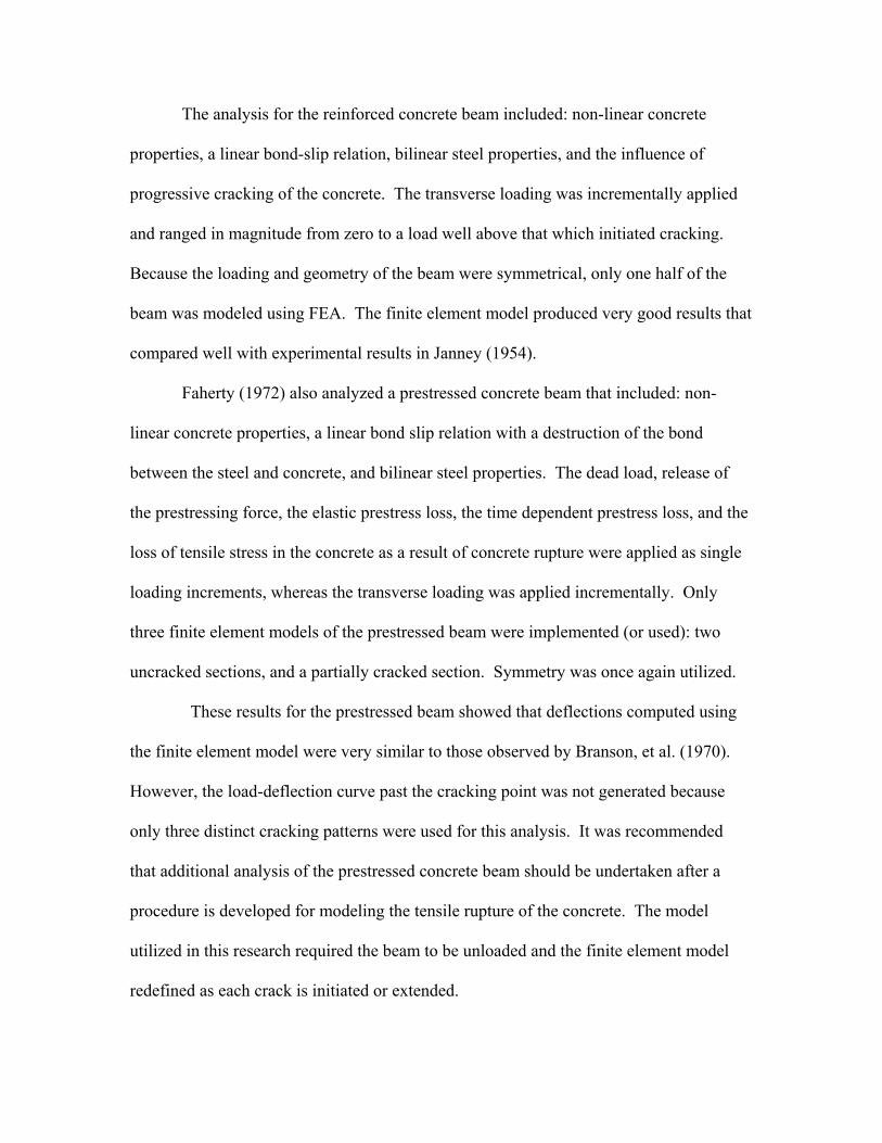
the beams tested were 10 in. and 18 in., respectively. As shown in Figure 3.1, the length
Figure 3.1 – Loading and Supports for the Beam (Buckhouse 1997)

of the beam was 15 ft.-6 in. with supports located 3 in. from each end of the beam
allowing a simply supported span of 15 ft. The mild steel flexural reinforcements used
were 3-#5 bars and shear reinforcements included #3 U-stirrups. Cover for the rebar was
set to 2 in. in all directions. The layout of the reinforcement is detailed in Figure 3.2.
Figure 3.2 – Typical Detail for Control Beam Reinforcement (Buckhouse 1997)
The steel yield stress, 28-day compressive stress of concrete, and area of steel
reinforcement are included in Table 3.1.
Table 3.1 – Properties for Steel and Concrete (Buckhouse 1997)
Area of Steel (in.2) 0.93
Yield Stress of Steel, fy (psi) 60,000
28-Day Compressive Strength of Concrete, fc'
(psi) 4,770

Two 50-kip capacity load cells were placed at third points, or 5 ft. from each
support on steel bearing plates (Figure 3.1). Data acquisition equipment was used to
record applied loading, beam deflection at the midspan, and strain in the internal flexural
reinforcement. The beam was loaded to flexural failure (Figure 3.3).
Figure 3.3 – Failure in Flexure (Buckhouse 1997)
Vertical cracks first formed in the constant moment region, extended upward, and then
out towards the constant shear region with eventual crushing of the concrete in the
constant moment region as shown in Figure 3.3. Test data for the beam is summarized in
Table 3.2.
The theoretical ultimate load for the beam was calculated to be 14,600 lbs
(Buckhouse 1997). Table 3.2 shows the experimental ultimate load determined was
16,310 lbs. The ultimate loading corresponded to the nominal flexural capacity of the
cross-section being reached. A plot of load versus deflection for control beam C1
(Buckhouse 1997) is shown in Figure 3.4.

Table 3.2 – Test data for control beam C1 (Buckhouse 1997)
Avg. Load at 1st Crack (lbs.) 4,500
Avg. Failure Load, P (lbs.) 16,310
Avg. Centerline Deflection at Failure
(in.) 3.65
Mode of Failure compression failure of concrete
0
2000
4000
6000
8000
10000
12000
14000
16000
18000
0 0.5 1 1.5 2 2.5 3 3.5 4 4.5
Avg. Centerline Deflection (in.)
Avg
. Loa
d, P
(lbs
.)
Figure 3.4 – Load vs. Deflection Curve for Beam C1 (Buckhouse 1997)
C1 theoretical ultimate load (14,600 lbs.)
A
B
C
Point A - First Cracking Point B - Steel Yielding Point C - Failure
Nonlinear Region
Linear Region
The plot shows the linear behavior before first cracking (point A). A second slope
corresponding to the cracked section is followed until point B where the flexural
reinforcement yields. The cracked moment of inertia with yielding internal
reinforcement then defines the stiffness until flexural failure at point C.
3.2 ANSYS Finite Element Model
The FEA calibration study included modeling a concrete beam with the dimensions and
properties corresponding to beam C1 tested by Buckhouse (1997). Due to the symmetry
in cross-section of the concrete beam and loading, symmetry was utilized in the FEA,
only one quarter of the beam was modeled.
To create the finite element model in ANSYS (SAS 2003) there are multiple tasks
that have to be completed for the model to run properly. Models can be created using
command prompt line input or the Graphical User Interface (GUI). For this model, the
GUI was utilized to create the model. This section describes the different tasks and
entries into used to create the FE calibration model.
3.2.1 Element Types
The element types for this model are shown in Table 3.3. The Solid65 element was used
to model the concrete. This element has eight nodes with three degrees of freedom at
each node – translations in the nodal x, y, and z directions. This element is capable of
plastic deformation, cracking in three orthogonal directions, and crushing. A schematic
of the element is shown in Figure 3.5.

Table 3.3 – Element Types For Working Model
Material Type ANSYS ElementConcrete Solid65
Steel Plates and Supports Solid45
Steel Reinforcement Link8
Figure 3.5 – Solid 65 Element (SAS 2003)
A Solid45 element was used for steel plates at the supports for the beam. This
element has eight nodes with three degrees of freedom at each node – translations in the
nodal x, y, and z directions. The geometry and node locations for this element is shown

in Figure 3.6. The descriptions for each element type are laid out in the ANSYS element
library (SAS 2003).
Figure 3.6 – Solid 45 Element (SAS 2003)
A Link8 element was used to model steel reinforcement. This element is a 3D
spar element and it has two nodes with three degrees of freedom – translations in the
nodal x, y, and z directions. This element is also capable of plastic deformation. This
element is shown in Figure 3.7.
3.2.2 Real Constants
The real constants for this model are shown in Table 3.4. Note that individual elements
contain different real constants. No real constant set exists for the Solid45 element.

Figure 3.7 – Link 8 Element (SAS 2003)
Table 3.4 – Real Constants For Calibration Model
Real Constant Set Element Type Constants
Real Constants for
Rebar 1
Real Constants for
Rebar 2
Real Constants for
Rebar 3 Material Number 0 0 0 Volume Ratio 0 0 0 Orientation Angle 0 0 0
1 Solid 65
Orientation Angle 0 0 0 Cross-sectional
Area (in.2) 0.31 2 Link8
Initial Strain (in./in.) 0
Cross-sectional
Area (in.2) 0.155 3 Link8
Initial Strain (in./in.) 0
Cross-sectional
Area (in.2) 0.11 4 Link8
Initial Strain (in./in.) 0
Cross-sectional
Area (in.2) 0.055 5 Link8
Initial Strain (in./in.) 0

Real Constant Set 1 is used for the Solid65 element. It requires real constants for
rebar assuming a smeared model. Values can be entered for Material Number, Volume
Ratio, and Orientation Angles. The material number refers to the type of material for the
reinforcement. The volume ratio refers to the ratio of steel to concrete in the element.
The orientation angles refer to the orientation of the reinforcement in the smeared model
(Figure 2.8c). ANSYS (SAS 2003) allows the user to enter three rebar materials in the
concrete. Each material corresponds to x, y, and z directions in the element (Figure 3.5).
The reinforcement has uniaxial stiffness and the directional orientation is defined by the
user. In the present study the beam is modeled using discrete reinforcement. Therefore,
a value of zero was entered for all real constants which turned the smeared reinforcement
capability of the Solid65 element off.
Real Constant Sets 2, 3, 4, and 5 are defined for the Link8 element. Values for
cross-sectional area and initial strain were entered. Cross-sectional areas in sets 2 and 3
refer to the reinforcement of 3-#5 bars. Due to symmetry, set 3 is half of set 2 because
one-half the center bar in the beam is cut off. Cross-sectional areas in sets 4 and 5 refer
to the #3 stirrups. Once again set 5 is half of set 4 because half of the stirrup at the mid-
span of the beam is cut off resulting from symmetry. A value of zero was entered for the
initial strain because there is no initial stress in the reinforcement.
3.2.3 Material Properties
Parameters needed to define the material models can be found in Table 3.5. As seen in
Table 3.5, there are multiple parts of the material model for each element.

Table 3.5 – Material Models For the Calibration Model
Material Model Number
Element Type Material Properties
Linear Isotropic EX 3,949,076 psi PRXY 0.3 Multilinear Isotropic Strain Stress Point 1 0.00036 1421.7 Point 2 0.0006 2233 Point 3 0.0013 3991 Point 4 0.0019 4656 Point 5 0.00243 4800 Concrete ShrCf-Op 0.3 ShrCf-Cl 1 UnTensSt 520 UnCompSt -1 BiCompSt 0 HydroPrs 0 BiCompSt 0 UnTensSt 0 TenCrFac 0
1 Solid65
Linear Isotropic EX 29,000,000 psi PRXY 0.3
2 Solid45
Linear Isotropic EX 29,000,000 psi PRXY 0.3 Bilinear Isotropic Yield Stss 60,000 psi Tang Mod 2,900 psi
3 Link8

Material Model Number 1 refers to the Solid65 element. The Solid65 element
requires linear isotropic and multilinear isotropic material properties to properly model
concrete. The multilinear isotropic material uses the von Mises failure criterion along
with the Willam and Warnke (1974) model to define the failure of the concrete. EX is
the modulus of elasticity of the concrete ( cE ), and PRXY is the Poisson’s ratio (ν ). The
modulus was based on the equation,
'57000c cE f= (3.1)
with a value of 'cf equal to 4,800 psi. Poisson’s ratio was assumed to be 0.3. The
compressive uniaxial stress-strain relationship for the concrete model was obtained using
the following equations to compute the multilinear isotropic stress-strain curve for the
concrete (MacGregor 1992)
2
0
1
cEf ε
εε
=
+
(3.2)
'
02 c
c
fE
ε = (3.3)
cfEε
= (3.4)
where:
f = stress at any strain ε , psi
ε = strain at stress f
0ε = strain at the ultimate compressive strength 'cf
The multilinear isotropic stress-strain implemented requires the first point of the curve to
be defined by the user. It must satisfy Hooke’s Law;

E σε
= (3.5)
The multilinear curve is used to help with convergence of the nonlinear solution
algorithm.
0
1000
2000
3000
4000
5000
6000
0 0.0005 0.001 0.0015 0.002 0.0025 0.003 0.0035
Strain (in./in.)
Stre
ss (p
si)
Figure 3.8 – Uniaxial Stress-Strain Curve
Figure 3.8 shows the stress-strain relationship used for this study and is based on
work done by Kachlakev, et al. (2001). Point 1, defined as '0.30 cf , is calculated in the
linear range (Equation 3.4). Points 2, 3, and 4 are calculated from Equation 3.2 with 0ε
obtained from Equation 3.3. Strains were selected and the stress was calculated for each
0ε
'0.30 cf
Strain at Ultimate Strength
cE
Ultimate Compressive Strength '
cf 5 4
3
2
1

strain. Point 5 is defined at 'cf and 0
.0.003 .in
inε = indicating traditional crushing strain
for unconfined concrete.
Implementation of the Willam and Warnke (1974) material model in ANSYS
requires that different constants be defined. These 9 constants are: (SAS 2003)
1. Shear transfer coefficients for an open crack;
2. Shear transfer coefficients for a closed crack;
3. Uniaxial tensile cracking stress;
4. Uniaxial crushing stress (positive);
5. Biaxial crushing stress (positive);
6. Ambient hydrostatic stress state for use with constants 7 and 8;
7. Biaxial crushing stress (positive) under the ambient hydrostatic stress state
(constant 6);
8. Uniaxial crushing stress (positive) under the ambient hydrostatic stress state
(constant 6);
9. Stiffness multiplier for cracked tensile condition.
Typical shear transfer coefficients range from 0.0 to 1.0, with 0.0 representing a
smooth crack (complete loss of shear transfer) and 1.0 representing a rough crack (no loss
of shear transfer). The shear transfer coefficients for open and closed cracks were
determined using the work of Kachlakev, et al. (2001) as a basis. Convergence problems
occurred when the shear transfer coefficient for the open crack dropped below 0.2. No
deviation of the response occurs with the change of the coefficient. Therefore, the
coefficient for the open crack was set to 0.3 (Table 3.4). The uniaxial cracking stress was
based upon the modulus of rupture. This value is determined using,
'7.5r cf f= (3.6)
The uniaxial crushing stress in this model was based on the uniaxial unconfined
compressive strength ( 'cf ) and is denoted as tf . It was entered as -1 to turn off the
crushing capability of the concrete element as suggested by past researchers (Kachlakev,
et al. 2001). Convergence problems have been repeated when the crushing capability
was turned on.
The biaxial crushing stress refers to the ultimate biaxial compressive strength
( 'cbf ). The ambient hydrostatic stress state is denoted as hσ . This stress state is defined
as:
1 ( )3h xp yp zpσ σ σ σ= + + (3.7)
where xpσ , ypσ , and zpσ are the principal stresses in the principal directions. The biaxial
crushing stress under the ambient hydrostatic stress state refers to the ultimate
compressive strength for a state of biaxial compression superimposed on the hydrostatic
stress state ( 1f ). The uniaxial crushing stress under the ambient hydrostatic stress state
refers to the ultimate compressive strength for a state of uniaxial compression
superimposed on the hydrostatic stress state ( 2f ). The failure surface can be defined
with a minimum of two constants, tf and 'cf . The remainder of the variables in the
concrete model are left to default based on these equations: (SAS 2003)
' '1.2cb cf f= (3.8)
'1 1.45 cf f= (3.9)
'2 1.725 cf f= (3.10)

These stress states are only valid for stress states satisfying the condition
'3h cfσ ≤ (3.11)
Material Model Number 2 refers to the Solid45 element. The Solid45 element is
being used for the steel plates at loading points and supports on the beam. Therefore, this
element is modeled as a linear isotropic element with a modulus of elasticity for the steel
( sE ), and poisson’s ratio (0.3).
Material Model Number 3 refers to the Link8 element. The Link8 element is
being used for all the steel reinforcement in the beam and it is assumed to be bilinear
isotropic. Bilinear isotropic material is also based on the von Mises failure criteria. The
bilinear model requires the yield stress ( yf ), as well as the hardening modulus of the steel
to be defined. The yield stress was defined as 60,000 psi, and the hardening modulus was
2900 psi.
Note that the density for the concrete was not added in the material model. For
the control beam in Buckhouse (1997), the LVDT’s used to measure deflection at mid-
span were put on the beam after it was set in the test fixture. Deflections were taken
relative to a zero deflection point after the self-weight was introduced. Therefore, the
self-weight was not introduced in this calibration model.
3.2.4 Modeling
The beam, plates, and supports were modeled as volumes. Since a quarter of the beam is
being modeled, the model is 93 in. long, with a cross-section of 5 in. x 18 in. The
dimensions for the concrete volume are shown in Table 3.6. The zero values for the Z-
coordinates coincide with the center of the cross-section for the concrete beam.

Table 3.6 – Dimensions for Concrete, Steel Plate, and Steel Support Volumes
ANSYS Concrete (in.) Steel Plate (in.) Steel Support (in.) X1,X2 X-coordinates 0 93 60 66 1.5 4.5 Y1,Y2 Y-coordinates 0 18 18 19 0 -1 Z1,Z2 Z-coordinates 0 5 0 5 0 5
The 93 in. dimension for the X-coordinates is the mid-span of the beam. Due to
symmetry, only one loading plate and one support plate are needed. The support is a 3 in.
x 5 in. x 1 in. steel plate, while the plate at the load point is 6 in. x 5 in. x 1 in. The
dimensions for the plate and support are shown in Table 3.6. The combined volumes of
the plate, support, and beam are shown in Figure 3.9. The FE mesh for the beam model
is shown in Figure 3.10.
Figure 3.9 – Volumes Created in ANSYS
Steel Support
Steel Loading Plate
Concrete Beam

Figure 3.10 – Mesh of the Concrete, Steel Plate, and Steel Support
Link8 elements were used to create the flexural and shear reinforcement.
Reinforcement exists at a plane of symmetry and in the beam. The area of steel at the
plane of symmetry is one half the normal area for a #5 bar because one half of the bar is
cut off. Shear stirrups are modeled throughout the beam. Only half of the stirrup is
modeled because of the symmetry of the beam. Figure 3.11 illustrates that the rebar
shares the same nodes at the points that it intersects the shear stirrups. The element type
number, material number, and real constant set number for the calibration model were set
for each mesh as shown in Table 3.7.
Steel Plate Element Width 1.25 in.
Concrete Element Length 1.5 in.
Concrete Element Width 1.25 in.
Concrete Element Height 1.2 in.
Steel Plate Element Length 1.5 in.
Steel Support Element Width 1.25 in.
Steel Support Element Length 1.5 in.

Figure 3.11 – Reinforcement Configuration
Table 3.7 – Mesh Attributes for the Model
Model Parts Element Type
Material Number
Real Constant Set
Concrete Beam 1 1 1 Steel Plate 2 3 N/A Steel Support 2 3 N/A Rebar at Center of Cross-Section 3 2 3 Rebar 2.5 in. of Cross-Section 3 2 2 Stirrup at Center of Beam 3 2 5 Other Stirrups 3 2 4
3.2.5 Meshing
To obtain good results from the Solid65 element, the use of a rectangular mesh is
recommended. Therefore, the mesh was set up such that square or rectangular elements
#3 Shear Stirrups
#5 Bar Reinforcement located 2.5 in. from the end of the Cross-Section
Shared nodes of Stirrups and Rebar
#5 Bar Reinforcement at Plane of Symmetry
Stirrup at Plane of Symmetry

were created (Figure 3.10). The volume sweep command was used to mesh the steel
plate and support. This properly sets the width and length of elements in the plates to be
consistent with the elements and nodes in the concrete portions of the model.
The overall mesh of the concrete, plate, and support volumes is shown in Figure
3.10. The necessary element divisions are noted. The meshing of the reinforcement is a
special case compared to the volumes. No mesh of the reinforcement is needed because
individual elements were created in the modeling through the nodes created by the mesh
of the concrete volume. However, the necessary mesh attributes as described above need
to be set before each section of the reinforcement is created.
3.2.6 Numbering Controls
The command merge items merges separate entities that have the same location. These
items will then be merged into single entities. Caution must be taken when merging
entities in a model that has already been meshed because the order in which merging
occurs is significant. Merging keypoints before nodes can result in some of the nodes
becoming “orphaned”; that is, the nodes lose their association with the solid model. The
orphaned nodes can cause certain operations (such as boundary condition transfers,
surface load transfers, and so on) to fail. Care must be taken to always merge in the order
that the entities appear. All precautions were taken to ensure that everything was merged
in the proper order. Also, the lowest number was retained during merging.

3.2.7 Loads and Boundary Conditions
Displacement boundary conditions are needed to constrain the model to get a unique
solution. To ensure that the model acts the same way as the experimental beam,
boundary conditions need to be applied at points of symmetry, and where the supports
and loadings exist.
The symmetry boundary conditions were set first. The model being used is
symmetric about two planes. The boundary conditions for both planes of symmetry are
shown in Figure 3.12.
Figure 3.12 – Boundary Conditions for Planes of Symmetry
Constraint in the z-direction
Constraint in the x-direction

Nodes defining a vertical plane through the beam cross-section centroid defines a plane
of symmetry. To model the symmetry, nodes on this plane must be constrained in the
perpendicular direction. These nodes, therefore, have a degree of freedom constraint UX
= 0. Second, all nodes selected at Z = 0 define another plane of symmetry. These nodes
were given the constraint UZ = 0.
The support was modeled in such a way that a roller was created. A single line of
nodes on the plate were given constraint in the UY, and UZ directions, applied as
constant values of 0. By doing this, the beam will be allowed to rotate at the support. The
support condition is shown in Figure 3.13.
Figure 3.13 – Boundary Condition for Support
Support roller condition to allow rotation

The force, P, applied at the steel plate is applied across the entire centerline of the
plate. The force applied at each node on the plate is one tenth of the actual force applied.
Figure 3.14 illustrates the plate and applied loading.
Figure 3.14 – Boundary Conditions at the Loading Plate
3.2.8 Analysis Type
The finite element model for this analysis is a simple beam under transverse loading. For
the purposes of this model, the Static analysis type is utilized.
The Restart command is utilized to restart an analysis after the initial run or load
step has been completed. The use of the restart option will be detailed in the analysis
portion of the discussion.
Loading Applied on the Plate
Boundary Conditions at Plate

The Sol’n Controls command dictates the use of a linear or non-linear solution for
the finite element model. Typical commands utilized in a nonlinear static analysis are
shown in Table 3.8.
Table 3.8 – Commands Used to Control Nonlinear Analysis
Analysis Options Small DisplacementCalculate Prestress Effects No Time at End of Loadstep 5120 Automatic Time Stepping On Number of Substeps 1 Max no. of Substeps 2 Min no. of Substeps 1 Write Items to Results File All Solution Items Frequency Write Every Substep
In the particular case considered in this thesis the analysis is small displacement and
static. The time at the end of the load step refers to the ending load per load step. Table
3.8 shows the first load step taken (e.g. up to first cracking). The sub steps are set to
indicate load increments used for this analysis. The commands used to control the solver
and output are shown in Table 3.9.
Table 3.9 – Commands Used to Control Output
Equation Solvers Sparse Direct Number of Restart Files 1 Frequency Write Every Substep
All these values are set to ANSYS (SAS 2003) defaults. The commands used for the
nonlinear algorithm and convergence criteria are shown in Table 3.10. All values for the
nonlinear algorithm are set to defaults.

Table 3.10 – Nonlinear Algorithm and Convergence Criteria Parameters
Line Search Off DOF solution predictor Prog Chosen Maximum number of iteration 100 Cutback Control Cutback according to predicted number of iter. Equiv. Plastic Strain 0.15 Explicit Creep ratio 0.1 Implicit Creep ratio 0 Incremental displacement 10000000 Points per cycle 13
Set Convergence Criteria Label F U Ref. Value Calculated calculated Tolerance 0.005 0.05 Norm L2 L2 Min. Ref. not applicable not applicable
The values for the convergence criteria are set to defaults except for the tolerances. The
tolerances for force and displacement are set as 5 times the default values. Table 3.11
shows the commands used for the advanced nonlinear settings. The program behavior
upon nonconvergence for this analysis was set such that the program will terminate but
not exit. The rest of the commands were set to defaults.
Table 3.11 – Advanced Nonlinear Control Settings Used
Program behavior upon nonconvergence Terminate but do not exit Nodal DOF sol'n 0 Cumulative iter 0 Elapsed time 0 CPU time 0

3.2.9 Analysis Process for the Finite Element Model
The FE analysis of the model was set up to examine three different behaviors: initial
cracking of the beam, yielding of the steel reinforcement, and the strength limit state of
the beam. The Newton-Raphson method of analysis was used to compute the nonlinear
response.
The application of the loads up to failure was done incrementally as required by
the Newton-Raphson procedure. After each load increment was applied, the restart
option was used to go to the next step after convergence. A listing of the load steps, sub
steps, and loads applied per restart file are shown in Table 3.12.
Table 3.12 – Load Increment for Analysis of Finite Element Model
Beginning Time
Time at End of Loadstep Load Step Sub Step
Load Increment
(lbs.) 0 5210 1 1 5210
5210 5220 2 10 10 5220 5300 3 16 5 5300 5400 4 20 5 5400 10000 5 92 50 10000 13000 6 30 100 13000 14000 7 10 100 14000 14500 8 50 10 14500 14700 9 20 10 14700 14800 10 20 5 14800 14900 11 100 1 14900 15000 12 10 10 15000 15100 13 10 10 15100 15200 14 50 2 15200 15300 15 20 5 15300 15600 16 150 2 15600 15900 17 150 2 15900 16200 18 150 2 16200 16300 19 50 2 16300 16382 20 41 2

The time at the end of each load step corresponds to the loading applied. For the first
load step the time at the end of the load step is 5210 referring to a load of, P, of 5210 lbs
applied at the steel plate.
The two convergence criteria used for the analysis were Force and Displacement.
These criteria were left at the default values up to 5210 lbs. However, when the beam
began cracking, convergence for the non-linear analysis was impossible with the default
values. The displacements converged, but the forces did not. Therefore, the convergence
criteria for force was dropped and the reference value for the Displacement criteria was
changed to 5. This value is then multiplied by the tolerance value of 0.05 to produce a
criterion of 0.25 during the nonlinear solution for convergence. A small criterion must be
used to capture correct response. This criteria was used for the remainder of the analysis.
As shown in Table 3.12, the steps taken to the initial cracking of the beam can be
decresed to one load increment to model/capture initial cracking. Once initial cracking of
the beam has been passed (5220 lbs), the load increments increased slightly until
subsequent cracking of the beam (14,000 lbs) as seen in Table 3.12. Once the yielding of
the reinforcing steel is reached, the load increments must be decreased again. Yielding of
the steel occurs at load step 13,400; therefore, the load increment sizes begin decreasing
further because displacements are increasing more rapidly. Eventually, the load
increment size is decreased to 2 lb. to capture the failure of the beam. Failure of the
beam occurs when convergence fails, with this very small load increment. The load
deformation trace produced by the analysis confirmed the failure load.

3.3 Results
The goal of the comparison of the FE model and the beam from Buckhouse (1997) is to
ensure that the elements, material properties, real constants and convergence criteria are
adequate to model the response of the member. Figure 3.4 shows the different
components that were analyzed for comparison: the linear region, initial cracking, the
nonlinear region, the yielding of steel, and failure.
3.3.1 Behavior at First Cracking
The analysis of the linear region can be based on the design for flexure given in
MacGregor (1992) for a reinforced concrete beam. Comparisons were made in this
region to ensure deflections and stresses were consistent with the FE model and the beam
before cracking occurred. Once cracking occurs, deflections and stresses become more
difficult to predict. The stresses in the concrete and steel immediately preceding initial
cracking were analyzed. The load at step 5210 was analyzed and it coincides with a load
of 5210 lbs. applied on the steel plate.
Calculations to obtain the concrete stress, steel stress and deflection of the beam
at a load of 5210 lbs. can be seen in Appendix A. A comparison of values obtained from
the FE model and Appendix A can be seen in Table 3.13. The maximums exist in the
constant-moment region of the beam during load application. This is where we expect
the maximums to occur. The results in Table 3.13 indicate that the FE analysis of the
beam prior to cracking is acceptable.

Table 3.13 – Deflection and Stress Comparisons At First Cracking
Model Extreme Tension Fiber Stress (psi)
Reinforcing Steel Stress
(psi)
Centerline Deflection
(in.)
Load at First Cracking
(lbs.)
Hand-Calculations 530 3024 0.0529 5118
ANSYS 536 2840 0.0534 5216
3.3.2 Behavior at Initial Cracking
The cracking pattern(s) in the beam can be obtained using the Crack/Crushing plot option
in ANSYS (SAS 2003). Vector Mode plots must be turned on to view the cracking in the
model.
The initial cracking of the beam in the FE model corresponds to a load of 5216 lbs
that creates stress just beyond the modulus of rupture of the concrete (520 psi) as shown
in Table 3.13. This compares well with the load of 5118 lbs calculated in Appendix A.
The stress increases up to 537 psi at the centerline when the first crack occurs. The first
crack can be seen in Figure 3.15. This first crack occurs in the constant moment region,
and is a flexural crack. Buckhouse (1997) reported first cracking at a load, P, of 4500 lbs
using visual detection.
3.3.3 Behavior Beyond First Cracking
In the non-linear region of the response, subsequent cracking occurs as more load is
applied to the beam. Cracking increases in the constant moment region, and the beam
begins cracking out towards the supports at a load of 8,000 lbs.

Figure 3.15 – 1st Crack of the Concrete Model
Significant flexural cracking occurs in the beam at 12,000 lbs. Also, diagonal tension
cracks are beginning to form in the model. This cracking can be seen in Figure 3.16.
3.3.4 Behavior of Reinforcement Yielding and Beyond
Yielding of steel reinforcement occurs when a force of 13,400 lbs. is applied. At this
point in the response, the displacements of the beam begin to increase at a higher rate as
more load is applied (Figure 3.4). The cracked moment of inertia, yielding steel, and
nonlinear concrete material, now defines the flexural rigidity of the member. The ability
of the beam to distribute load throughout the cross-section has diminished greatly.
Therefore, greater deflections occur at the beam centerline.
1st Crack in Concrete Beam

Figure 3.16 – Cracking at 8,000 and 12,000 lbs.
Figure 3.17 shows successive cracking of the concrete beam after yielding of the
steel occurs. At 15,000 lbs., the beam has increasing flexural cracks, and diagonal
tension cracks. Also, more cracks have now formed in the constant moment region. At
16,000 lbs., cracking has reached the top of the beam, and failure is soon to follow.
Flexural Cracks
Diagonal Tension Cracks

Figure 3.17 – Increased Cracking After Yielding of Reinforcement
3.3.5 Strength Limit State
At load 16,382 lbs., the beam no longer can support additional load as indicated by an
insurmountable convergence failure. Severe cracking throughout the entire constant
moment region occurs (see Figure 3.18). The deflections at the analytical failure load of
the control beam were compared with the finite element model as shown in Table 3.14.
Multiple cracks occurring
Increasing Diagonal Tension Cracks

Figure 3.18 – Failure of the Concrete Beam
Table 3.14 – Deflections of Control Beam (Buckhouse 1997) vs. Finite Element Model At Ultimate Load
Beam Load (lb.)Centerline Deflection
(in.) C1 16310 3.65
ANSYS 16310 3.586
The deflection of the finite element model was within 2% of the control beam at the same
load at which the control beam failed.
Excessive cracking and of the beam in the constant moment region
Diagonal Tension Cracking

3.3.6 Load-Deformation Response
The full nonlinear load-deformation response can be seen in Figure 3.19. This response
was calibrated by setting the tolerances so that the load-deformation curve fits to the
curve from Buckhouse (1997). The response calculated using FEA is plotted upon the
experimental response from Buckhouse (1997). The entire load-deformation response of
the model produced compares well with the response from Buckhouse (1997). This gave
confidence in the use of ANSYS (SAS 2003) and the model developed. The approach
was then utilized to analyze a prestressed concrete beam.
0
2000
4000
6000
8000
10000
12000
14000
16000
18000
0 0.5 1 1.5 2 2.5 3 3.5 4 4.5
Avg. Centerline Deflection (in.)
Avg
. Loa
d, P
(lbs
.)
Figure 3.19 – Load vs. Deflection Curve Comparison of ANSYS and Buckhouse (1997)
Buckhouse (1997)
FEA
C1 theoretical ultimate load (14,600 lbs.)

CHAPTER 4
PRESTRESSED CONCRETE BEAM MODEL
4.0 Introduction
This chapter discusses the finite element modeling of a prestressed concrete beam. The
prestressed beam has the same dimensions as the experimental beam modeled by
Buckhouse (1997). In this case, the reinforcement in the beam is different. The shear
stirrups are included as discussed in the calibration model. However, no mild-steel
flexural reinforcement was used. The beam was prestressed using ½ in. diameter 270 ksi
7-wire strands as opposed to the #5 60 ksi mild-steel reinforcement. All the necessary
steps taken to create the model and the analysis used for the prestressed beam are
explained in detail.
4.1 Finite Element Model
The finite element model that was used for analysis of the prestressed concrete beam is
very similar to the calibration model. Many of the steps taken to model the prestressed
concrete beam were the same as the calibration model and can be found in chapter 3.
The rest of this chapter will discuss the steps taken that were different from those
in the calibration model. These steps include definition of real constants, material
properties, and the parameters for the nonlinear analysis.

4.1.1 Real Constants
The real constants for the concrete element were left untouched because the modeling of
the concrete has not changed. Also, the constants for the Link8 element designated to the
stirrups used in the model were left unchanged. However, the real constants for the
Link8 element for the flexural reinforcement has changed. Since the beam is now using
prestressing steel, the cross-sectional area of the steel has changed, and an initial strain
due to prestressing is now added to the element. The change in area and strain is shown
in Table 4.1.
Table 4.1 – Real Constants for Prestressed Beam
Real Constant Set Element Type Constants
Cross-sectional Area (in.2) 0.153
2 Link8 Initial Strain
(in./in.) 0.001903
Cross-sectional Area (in.2) 0.0765
3 Link8 Initial Strain
(in./in.) 0.001903
The cross-sectional area for real constant set 2 is the area of an equivalent ½ in. diameter
7-wire strand. The cross-sectional area for real constant set 3 is half of real constant set
2, because it is at a point of symmetry on the model.
The initial strains for each real constant set were determined from the effective
prestress ( pef ) and the modulus of elasticity ( psE ). An example of this can be seen in
Appendix B. This prestress level is too low and not suitable for practical use. It was

utilized to prevent any convergence problems occurring from bursting and significant
cracking near the support as the prestrain is applied.
4.1.2 Material Properties
The material properties for the shear reinforcement steel, steel plates at loading points,
and steel support plates are the same. Density was added to the concrete material
property so the self-weight of the concrete beam could be taken into account.
The material properties for the prestressing steel have been changed from bilinear
isotropic to multilinear isotropic following the von Mises failure criteria. The
prestressing steel was modeled using a multilinear stress-strain curve developed using the
following equations,
0.008 :psε ≤ 28,000ps psf ε= ( )ksi (4.1)
>0.008:psε 0.075268 <0.98 ( )0.0065ps pu
ps
f f ksiε
= −−
(4.2)
The values entered into ANSYS (SAS 2003) for the stress-strain curve are given in Table
4.2 and Figure 4.1 shows the stress-strain behavior of the prestressing steel.
4.1.3 Solution
Most of the parameters used to control the solution are the same as those used for the
calibration model. The only changes made were as follows. First, no point loads are
applied in the first load step, due to the fact that the initial prestrain is applied. Second,
the time at the end of the prestrain application load step is 1. Third, the self-weight was
added in a load step. The addition of the self-weight is done by applying gravitational

acceleration of 386.4 in/s2 in the global y-direction. A mass density was entered in as a
function of the gravitational acceleration (Density/g).
Table 4.2 – Values for Multilinear Isotropic Stress-Strain Curve
Strain Stress Strain Stress Strain Stress Strain Stress 0 0 0.0101 247.1667 0.0123 255.069 0.0145 258.625
0.008 224 0.0103 248.2632 0.0125 255.5 0.0147 258.85370.0083 226.3333 0.0105 249.25 0.0127 255.9032 0.0149 259.07140.0085 230.5 0.0107 250.1429 0.0129 256.2813 0.0151 259.27910.0087 233.9091 0.0109 250.9545 0.0131 256.6364 0.0171 260.92450.0089 236.75 0.0111 251.6957 0.0133 256.9706 0.0189 261.95160.0091 239.1538 0.0113 252.375 0.0135 257.2857 0.0215 2630.0093 241.2143 0.0115 253 0.0137 257.5833 0.0259 264.1340.0095 243 0.0117 253.5769 0.0139 257.8649 0.0301 264.8220.0097 244.5625 0.0119 254.1111 0.0141 258.1316 0.0099 245.9412 0.0121 254.6071 0.0143 258.3846
0
50
100
150
200
250
300
0 0.005 0.01 0.015 0.02 0.025 0.03 0.035
Strain (in./in.)
Stre
ss (k
si)
Figure 4.1 – Stress-Strain Curve for 270 ksi strand

4.1.4 Analysis Process for the Finite Element Model
Analysis for the prestressed concrete beam was very similar to the calibration model.
However, different load step and restart points were used. The first load step taken was
to produce the camber in the concrete beam due to the prestress. The second load step
was the addition of the self-weight. From that point on, the concrete was modeled to the
point of cracking, yielding of the prestress steel ( 0.85 puf ), and eventual failure. A listing
of the load steps, sub steps, and loads applied per restart file are shown in Table 4.3.
Table 4.3 – Load Increments for the Analysis of the Prestressed Beam Model
Beginning Time
Time at End of
LoadstepLoad Step Sub Step
Load Increment
(lbs.) 0 1 1 1 Prestress1 2 2 1 386.4 2 7840 3 1 7840
7840 7900 4 30 2 7900 8500 5 12 50 8500 10000 6 15 100 10000 20000 7 100 100 20000 25000 8 100 50 25000 27000 9 200 10 27000 28000 10 100 10 28000 28823 11 412 2
When the analysis reaches the point of initial cracking, the force convergence
criteria is dropped, and the reference value of the displacement criteria is 5. From this
point, the load increments are decreased to 100 lbs. to capture the initial cracking of the
beam. When yielding of the steel occurs, the load increments are decreased to 10 lb.
Finally, load increments are decreased to 2 lb. until unresolvable convergence failure of
the non-linear algorithm occurs.

4.2 Results
The analysis yielded results for seven distinct points on the load-deflection application of
the prestressed concrete beam and the full nonlinear load-deformation response. As seen
in Figure 4.2, these distinct points are: effective prestress, addition of self-weight, zero
deflection, decompression, initial cracking, steel yielding ( 0.85 puf ), and failure.
4.2.1 Application of Effective Prestress
Calculation of the effective prestress for the beam can be found in Appendix B. The
deflections computed using hand calculations and FE analysis due to the prestress force is
shown in Table 4.4.
Table 4.4 – Analytical Results
ANSYS Hand Calculations
Centerline Deflection at Effective Prestress (in.) -0.0323 -0.0341
Top Fiber Stress at Effective Prestress (psi) 156.05 163.04
Deflection at Application of Self-Weight (in.) -0.0211 -0.0229
Top Fiber Stress at Self-Weight (psi) 36.97 45.86
Zero Deflection Load (lbs.) 2055 2126
Decompression Load (lbs.) 2817 2858
Initial Cracking Load (lbs.) 7850 7538
Prestress at Failure Load (psi) 264,822 254,520
Failure Load (lbs.) 28,823 27,587

-5000
0
5000
10000
15000
20000
25000
30000
35000
-0.50 0.00 0.50 1.00 1.50 2.00 2.50 3.00 3.50 4.00
Centerline Deflection (in.)
Load
, P (l
bs.)
0
1000
2000
3000
4000
5000
6000
7000
8000
-0.04 -0.02 0.00 0.02 0.04 0.06 0.08 0.10
Centerline Deflection (in.)
Load
, P (l
bs.)
Figure 4.2 – Load vs. Deflection Curve for Prestressed Concrete Model
Initial Cracking
Steel Yielding
Failure
Zero Deflection
DecompressionSelf-Weight
Initial Cracking
Linear Region
Secondary Linear Region
SEE FIGURE BELOW
Prestressing

The deflection in ANSYS (SAS 2003) corresponds well to the calculated value. The
stresses in the extreme fibers were looked at in the beam also. Since camber is occurring
in the beam (Figure 4.3), the controlling stress exists in the extreme top fiber.
Figure 4.3 – Deflection due to prestress
The hand-calculated top fiber stress and the top fiber stress found using FEA are also
shown in Table 4.4. The values correlate very well.
A phenomenon that occurred when the prestress was added was bursting in the
concrete where the prestress force is being applied. This phenomenon can be seen in
Figure 4.4. The contour plot shows that at the time of prestressing, there is a maximum
Camber due to prestressing force
Deflection (in.)

stress in the concrete where bursting occurs. The bursting phenomenon is explained in
detail in Nawy (2000).
Figure 4.4 – Bursting Phenomenon
Also, localized cracking occurs in the concrete, as shown in Figure 4.5. However, this
does not impact the solution because no other cracking occurs in that area after the initial
application of prestress. When a traditional level of prestress was applied
( 159,840pef psi= ), bursting zone cracking was extensive – a converged solution was not
possible to obtain. This is the reason for the reduction in pef by the factor of 3.
Bursting Effect at Center of Beam
Tendon Level

Figure 4.5 – Localized Cracking From Effective Prestress Application
4.2.2 Self-Weight
Adding the self-weight gives a deflection value which corresponds well to the calculated
deflection in Appendix B (Table 4.4). The FEA calculated top fiber stress at this stage
also correlates well with hand-calculations.
4.2.3 Zero Deflection
Hand-calculations (Appendix B) determined the load at which the deflection of the
centerline was zero. Table 4.4 indicates very good correlation between the hand
calculated values and the FEA.
Cracking that occurs from bursting

4.2.4 Decompression
One definition of decompression denotes the point of loading where the stress at the
bottom fiber of the concrete beam moves from compression due to the prestress to
tension from superimposed loading. Table 4.4 indicates very good correlation at this
level of loading as well.
4.2.5 Initial Cracking
Initial cracking is defined to be the loading at which the extreme tension fiber reaches the
modulus of rupture. Initial cracking of the beam in the FE model occurs at load 7850 lbs.
The hand-calculated load where cracking occurs is 7538 lbs. (Table 4.4 and Appendix B).
This is just past the modulus of rupture of the beam of 520 psi. The stress increases up to
539 psi at the centerline when the first crack occurs. This first crack occurs in the
constant moment region, and is a flexural crack.
4.2.6 Secondary Linear Region
In the secondary linear region of the response, significantly more cracking occurs as more
load is applied the beam as seen in Figure 4.6. Cracking increases in the constant
moment region, and the beam begins cracking out towards the supports with at a load of
12,000 lbs. Additional flexural cracking occurs in the beam at 20,000 lbs. Also, diagonal
tension cracks are beginning to form in the model.

Figure 4.6 – Cracking at 12,000 and 20,000 lbs.
4.2.7 Behavior of Steel Yielding and Beyond
Yielding of the prestress steel is defined as 0.85 puf for this model. Figure 4.2 illustrates
the load level at the point of yielding of the prestress steel. At this point in the response,
the displacements of the beam begin to increase at a higher rate as more load is applied.
The ability of the beam to distribute load throughout the cross-section has diminished
Flexural CracksBursting Cracks
Diagonal Tension Cracks

greatly. Therefore, greater deflections occur at the beam centerline. Increasing flexural
cracks and diagonal tension cracks form as the beam approaches failure (Figure 4.6).
4.2.8 Flexural Limit State
At a load of 28,823 lbs. unresolvable non-convergence of the nonlinear algorithm occurs,
indicating that cracking throughout the entire constant moment region has occurred.
Figure 4.7 illustrates the excessive cracking in the beam.
Figure 4.7 – Cracking at Flexural Capacity
Cracking at Failure

Hand calculations (Appendix B) predicted that the flexural capacity of the beam would
correspond to 27,587 lbs. (Table 4.4). The FEA prediction (28,823 lbs. in Table 4.4)
corresponds very well with the hand calculations. The stress in the prestressing steel at
failure predicted using FEA was 264,822 psi (Table 4.4). Using strain compatibility the
stress in the prestressing steel at failure was 254,520 psi (Appendix B), which
corresponds well to the FEA prediction.
The application of the moderate prestressing, 3pef , assumed in the present case
increased the limit load for the beam from 16,310 lbs. (Chapter 3) to 28,823 lbs. (near
doubling). The benefits of prestressing are apparent.

CHAPTER 5
CONCLUSIONS AND RECOMMENDATIONS
5.0 Introduction
The use of the finite element method to analyze reinforced and prestressed concrete
beams was evaluated. A reinforced concrete beam model was calibrated to experimental
data, and predictions of initial cracking, yielding of the steel and flexural failure of the
beam were compared to the experimental results. A prestressed concrete beam model
was also created. Initial prestress, addition of self-weight, zero deflection point,
decompression, initial cracking, yielding of steel, and flexural failure were then studied
and compared to theoretical values obtained via accepted methods of hand calculation.
5.1 Conclusions
The following conclusions can be stated based on the evaluation of the analyses of the
calibration model and the prestressed concrete beam.
(1) Deflections and stresses at the centerline along with initial and progressive
cracking of the finite element model compare well to experimental data obtained
from a reinforced concrete beam.
(2) The failure mechanism of a reinforced concrete beam is modeled quite well using
FEA, and the failure load predicted is very close to the failure load measured
during experimental testing.

(3) For the prestressed concrete beam, camber due to the initial prestress force and
after application of the self-weight of the beam compares well to hand-computed
values. Also, a bursting effect was seen in the FE model.
(4) Deflections and stresses at the zero deflection point and decompression are
modeled well using a finite element package.
(5) The load applied to cause initial cracking of the prestressed concrete beam
compares well with hand calculations.
(6) Flexural failure of the prestressed concrete beam is modeled well using a finite
element package, and the load applied at failure is very close to hand calculated
results.
5.2 Recommendations for Future Work
The literature review and analysis procedure utilized in this thesis has provided useful
insight for future application of a finite element package as a method of analysis. To
ensure that the finite element model is producing results that can be used for study, any
model should be calibrated with good experimental data. This will then provide the
proper modeling parameters needed for later use.
While modeling the prestressed beam, relaxation losses due to prestress, creep,
shrinkage, and elastic shortening were lumped together in a single load step. Individual
modeling of these losses could be included in future research. Many prestressed
structural components have non-symmetric geometries and loadings. Therefore, non-
symmetric geometries and loadings should be analyzed using finite element analysis with

prestress for further study. Higher strength concrete, the bursting effect, and the transfer
length of the prestressing steel are all candidates for future research.

REFERENCES
American Concrete Institute (1978), Douglas McHenry International Symposium on Concrete and Concrete Structures, American Concrete Institute, Detroit, Michigan. Branson, D.E.; Meyers, B.L.; and Kripanarayanan, K.M. (1970), “Loss of Prestress, Camber and Deflection of Noncomposite and Composite Structures Using Different Weight Concrete,” Iowa State Highway Comission, Report No. 70-6, Aug. Buckhouse, E.R. (1997), “External Flexural Reinforcement of Existing Reinforced Concrete Beams Using Bolted Steel Channels,” Master’s Thesis, Marquette University, Milwaukee, Wisconsin. Faherty, K.F. (1972), “An Analysis of a Reinforced and a Prestressed Concrete Beam by Finite Element Method,” Doctorate’s Thesis, University of Iowa, Iowa City. Fanning, P. (2001), “Nonlinear Models of Reinforced and Post-tensioned Concrete Beams,” Electronic Journal of Structural Engineering, University College Dublin, Earlsfort Terrace, Dublin 2, Ireland, Sept.12. Kachlakev, D.I.; Miller, T.; Yim, S.; Chansawat, K.; Potisuk, T. (2001), “Finite Element Modeling of Reinforced Concrete Structures Strengthened With FRP Laminates,” California Polytechnic State University, San Luis Obispo, CA and Oregon State University, Corvallis, OR for Oregon Department of Transportation, May. Janney, J.R. (1954), “Nature of Bond in Pre-tensioned Prestressed Concrete,” Journal of the ACI, Proceedings, Vol.50, No.5, May. MacGregor, J.G. (1992), Reinforced Concrete Mechanics and Design, Prentice-Hall, Inc., Englewood Cliffs, NJ. McCurry, D., Jr. and Kachlakev, D.I (2000), “Strengthening of Full Sized Reinforced Concrete Beam Using FRP Laminates and Monitoring with Fiber Optic Strain Guages” in Innovative Systems for Seismic Repair and Rehabilitation of Structures, Design and Applications, Technomic Publishing Co., Inc., Philadelphia, PA, March. Nawy, E.G., (2000), Prestressed Concrete: A Fundamental Approach, Prentice-Hall, Inc., Upper Saddle River, NJ SAS (2003) ANSYS 7.1 Finite Element Analysis System, SAS IP, Inc. Shing, P.B. and Tanabe, T.A., Ed. (2001), Modeling of Inelastic Behavior of RC Structures Under Seismic Loads, American Society of Civil Engineers.

Tavarez, F.A., (2001), “Simulation of Behavior of Composite Grid Reinforced Concrete Beams Using Explicit Finite Element Methods,” Master’s Thesis, University of Wisconsin-Madison, Madison, Wisconsin. Willam, K., and Tanabe, T.A., Ed. (2001), Finite Element Analysis of Reinforced Concrete Structures, American Concrete Institute, Farmington Hills, MI. Willam, K.J. and Warnke, E.P. (1974), “Constitutive Model for Triaxial Behaviour of Concrete,” Seminar on Concrete Structures Subjected to Triaxial Stresses, International Association of Bridge and Structural Engineering Conference, Bergamo, Italy, p.174.

APPENDICES
The following appendices have been included for reference:
PAGE
Appendix A: Theoretical Calculations for Calibration Model . . . . . . . . . . . . . . . . 69
Appendix B: Theoretical Calculations for Prestressed Model . . . . . . . . . . . . . . . . 73

Appendix A

Analysis of reinforced concrete beam for flexure at applied load of 5210 lbs.
Figure A.1 – Loading of Beam with Supports
Maximum Moment
The moment that occurs from the existing forces
max (5210 .)(60 .) 312,600 . .M lbs in lb in= = −
Material Properties
The gross moment of inertia
3 3 41 1 (10 .)(18 .) 486012 12GI bh in in in= = =
The modulus of elasticity of the concrete
'57,000 57,000 4800 3,949,076c cE f psi= = =
The modulus of rupture
'7.5 7.5 4800 520r cf f psi= = =
3”
60”60”
3”
5210 lbs. 5210 lbs.
60”

Stresses in Concrete and Steel
The stresses at the extreme tension fiber are calculated using a transformed moment of
inertia of the concrete and steel reinforcement
Figure A.2 – Transformed Cross-Section
Transformed area of steel
2( ) 8 8(3)(0.31) 7.44s t sA A in= = =
23.72in distributed on each side of the concrete cross-section
Calculate the distance from the top fiber to the neutral axis of the transformed moment of
inertia
21 1 2 2
21 2
(18 .)(10 .)(9 .) (2)(3.72 . )(15.5 .) 9.258 .(18 .)(10 .) (2)(3.72 . )
A y A y in in in in iny inA A in in in+ +
= = =+ +
The transformed moment of inertia
2 2tr G Concrete Steel
I I Ad Ad = + +
4 2 2 2 44860 . (10 .)(18 .)(0.258 .) (2)(3.72 . )(6.242 .) 5162 .in in in in in in in = + + =
The stress at the extreme tension fiber is then calculated
18”
3.72 in2
15.5”Ybar
10”

4
(312,600 . .)(8.742 .)5162 .
bct
tr
My lb in infI in
−= = = 530 psi
The stress in the steel at this point is calculated
4
(312,600 . .)(6.242 .) (8)5162 .
bs
tr
My lb in infI in
η −= = = 3024 psi
Deflections
The deflection at the centerline of the concrete beam at load 5210 lbs.
2 2max (3 4 )
24 tr
Pa l aEI
∆ = −
2 24
(5210 .)(60 .) (3(180 .) 4(60 .) )24(3,949,076)(5162 . )
lb in in inin
= − = 0.0529 in.
Loads
The load at first cracking
bct
tr
MyfI
=
4
(60 .)(8.742 .)5205162 .
P in inpsiin
=
P = 5117 lbs.

Appendix B

Analysis of Deflection for the Prestressed Concrete Beam
Figure B.1 – Typical Prestressed Concrete Beam with Supports
Effective Prestress
270,000puf psi=
0.74 0.74(270,000 ) 199,800pi puf f psi psi= = =
0.80 0.80(199,800 ) 159,840pe pif f psi psi= = =
159,840 / 3psi = 53,280 psi
Deflections
Deflection due to prestress
2 2
4
(24,456 .)(6.6 .)(180 .)8 8(3,949,076 )(4860 . )c
c c
Pel lb in inE I psi in
δ = − = − = -0.03406 in.
Deflection due to self-weight
4 45 5(15.624 )(180 .)384 384(3,949,076 )(4860)
wl pli inEI psi
δ = = = 0.1113 in.
Deflection after prestress and self-weight is applied
0.03406 0.01113 0.02293 .net c sw inδ δ δ= + = − + = −
3”
60”60”
3”
60”
cgs
cgc
ec PP

Stresses
Stress in extreme top fiber of the beam after initial prestress
2 2 2
24,456 . (6.6 .)(9 .)(1 ) (1 )180 . 27 .
t e t
c
P ec lb in infA r in in
= − − = − − = 163.04 psi (T)
'0.45 0.45(4800 ) 2160 ( ), . .c cf f psi psi T O K< = = =
Stress in extreme top fiber of the beam after self-weight
2 2 2 3
24,456 . (6.6 .)(9 .) 63277.2 . .(1 ) (1 )180 . 27 . 540 .
t e t Tt
c
P ec M lb in in lb infA r S in in in
−= − − − = − − −
= 45.86 psi (T)
'0.45 0.45(4800 ) 2160 ( ), . .c cf f psi psi T O K< = = =
Stress in extreme bottom fiber after prestress and self-weight
2 2 2 3
24,456 . (6.6 .)(9 .) 63,277.2 . .(1 ) (1 ) 317.6 ( )180 . 27 . 540 .
e b Tb
c b
P ec M lb in in lb inf psi CA r S in in in
−= − + + = − + + = −
'12 12 4800 831.4 ( ), . .t cf f psi psi T O K< = = =
Loads
Load needed to cause zero deflection
2 24
(60 .)0.02293 . (3(180 .) 4(60 .) )24(3,949,076 )(4860 . )
P inin in inpsi in
= −
P = 2126 lbs.
Calculated Load of Application at Decompression
2(1 )e b Tb
c b
P ec M MyfA r S I
= − + + +

(60 .)(9 .)0 317.64
P in inpsi= − +
P = 2858 lbs.
Determine the force of first cracking based on the cracked moment
2
( )cr D L r b eb
rM M M f S P ec
= + = + +
23 27 .63,277.2 . . (60 .) (520 )(540 . ) 24,456 .(6.6 . )
9 .inlb in P in psi in lbs inin
− + = + +
P = 7538 lbs.
Ultimate Strength Design by Strain Compatibility
153,280 .0.0019029 .28,000,000
pepe
ps
f psi ininE psi
ε ε= = = =
23(0.153 . )(53,280 ) 24,456 .eP in psi lbs= =
2 2
2 2 2 2
24,456 . (6.6 .) .(1 ) (1 ) 0.0000899 .(180 . )(3,949,076 ) 27 .e
decompc c
P e lbs in ininA E r in psi in
ε ε= = + = + =
Assume 205,000 psi for iteration process:
2
'
3(0.153 . )(205,000 ) 2.30625 .0.85 0.85(4800 )(10 .)
ps ps
c
A f in psia inf b psi in
= = =
1 0.85 0.05 0.80β = − =
1
2.30625 2.8828 .0.8
ac inβ
= = =
15.6 .d in=
315.6 . 2.8828 .. .( ) 0.003 ( ) 0.0132342. .2.8828 .c
d c in inin inin inc in
ε ε − −= = =
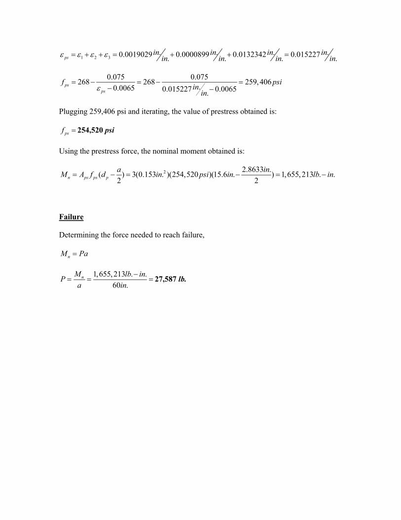
1 2 3. . . .0.0019029 0.0000899 0.0132342 0.015227. . . .ps
in in in inin in in inε ε ε ε= + + = + + =
0.075 0.075268 268 259,406.0.0065 0.015227 0.0065.ps
ps
f psiininε
= − = − =− −
Plugging 259,406 psi and iterating, the value of prestress obtained is:
psf = 254,520 psi
Using the prestress force, the nominal moment obtained is:
2 2.8633 .( ) 3(0.153 . )(254,520 )(15.6 . ) 1,655,213 . .2 2n ps ps pa inM A f d in psi in lb in= − = − = −
Failure
Determining the force needed to reach failure,
nM Pa=
1,655,213 . .60 .
nM lb inPa in
−= = = 27,587 lb.

Marquette University
This is to certify that we have examined
this copy of the masters thesis by
Anthony J. Wolanski
and have found that it is complete and satisfactory in all respects.
This thesis has been approved by: Director Christopher M. Foley, Ph.D., P.E. Stephen M. Heinrich, Ph.D. Baolin Wan, Ph.D.


