Download - FINITE ELEMENT SOLUTIONS TO INVERSE …

FINITE ELEMENT SOLUTIONS TO INVERSE ELECTROCARDIOGRAPHY
by
Dafang Wang
A dissertation submitted to the faculty of The University o f Utah
in partial fulfillment o f the requirements for the degree of
D octor of Philosophy
in
Computer Science
School o f Computing
The University o f Utah
December 2012

Copyright © Dafang Wang 2012
All Rights Reserved

The U n i v e r s i t y o f Ut ah G r a d u a t e S c h o o l
STATEMENT OF DISSERTATION APPROVAL
The dissertation of Dafang Wang
has been approved by the following supervisory committee members:
Christopher R. Johnson Co-Chair May 31, 2012Date Approved
Robert M. Kirby Co-Chair June 7, 2012Date Approved
Rob S. MacLeod Member May 31, 2012Date Approved
Ross Whitaker Member June 7, 2012Date Approved
Dana Brooks Member June 10, 2012Date Approved
and by Alan Davis Chair of
the Department of _____________________School of Computing
and by Charles A. Wight, Dean of The Graduate School.

ABSTRACT
Inverse Electrocardiography (ECG) aims to noninvasively estimate the electrophysiolog-
ical activity of the heart from the voltages measured at the body surface, with promising
clinical applications in diagnosis and therapy. The main challenge o f this emerging tech
nique lies in its mathematical foundation: an inverse source problem governed by partial
differential equations (PDEs) which is severely ill-conditioned. Essential to the success of
inverse ECG are computational methods that reliably achieve accurate inverse solutions
while harnessing the ever-growing complexity and realism of the bioelectric simulation.
This dissertation focuses on the formulation, optimization, and solution o f the inverse ECG
problem based on finite element methods, consisting of two research thrusts.
The first thrust explores the optimal finite element discretization specifically oriented
towards the inverse ECG problem. In contrast, most existing discretization strategies are
designed for forward problems and may become inappropriate for the corresponding inverse
problems. Based on a Fourier analysis of how discretization relates to ill-conditioning, this
work proposes refinement strategies that optimize approximation accuracy o f the inverse
ECG problem while mitigating its ill-conditioning. To fulfill these strategies, two refinement
techniques are developed: one uses hybrid-shaped finite elements whereas the other adapts
high-order finite elements.
The second research thrust involves a new methodology for inverse ECG solutions
called PDE-constrained optimization, an optimization framework that flexibly allows convex
objectives and various physically-based constraints. This work features three contributions:
(1) fulfilling optimization in the continuous space, (2) formulating rigorous finite element
solutions, and (3) fulfilling subsequent numerical optimization by a primal-dual interior-
point method tailored to the given optimization problem's specific algebraic structure. The
efficacy o f this new method is shown by its application to localization o f cardiac ischemic
disease, in which the method, under realistic settings, achieves promising solutions to
a previously intractable inverse ECG problem involving the bidomain heart model. In
summary, this dissertation advances the computational research of inverse ECG, making it
evolve toward an image-based, patient-specific modality for biomedical research.

To My Beloved Father and Mother, Wang Haicheng and Mao Zhiyun

CONTENTS
A B S T R A C T ..................................................................................................................................... iii
L IS T O F F IG U R E S .................................................................................................................... v iii
L IS T O F T A B L E S ......................................................................................................................... x iii
A C K N O W L E D G E M E N T S ......................................................................................................x iv
C H A P T E R S
1......I N T R O D U C T I O N ............................................................................................................... 1
1.1 Thesis Statem ent............................................................................................................... 21.1.1 Goal 1: Finite Element Discretization S tra te g y ............................................ 21.1.2 Goal 2: Adaptation o f h /p-type Finite Element Refinement ................... 31.1.3 Goal 3: Inverse Solution by PDE-Constrained O ptim ization ................... 31.1.4 Goal 4: Localization of Myocardial Is ch em ia ................................................ 4
1.2 Contributions .................................................................................................................... 41.3 O rgan ization ....................................................................................................................... 51.4 Notation and A bbrev ia tion ............................................................................................ 5
2. B A C K G R O U N D .................................................................................................................. 7
2.1 Bioelectric B ack grou n d ................................................................................................... 72.1.1 Cardiac Electrophysiology..................................................................................... 72.1.2 Bioelectric Models in E lectrocardiography..................................................... 8
2.1.2.1 Torso Conduction Model ........................................................................... 92.1.2.2 Bidomain Heart Model ................................................................................ 10
2.1.3 Myocardial Ischemia and Its Modeling ............................................................. 112.2 Mathematical Background ............................................................................................ 13
2.2.1 Galerkin Finite Element Method for Elliptic Equations ............................. 132.2.1.1 Boundary Condition Enforcement .......................................................... 152.2.1.2 Finite Element Refinement ......................................................................... 15
2.2.2 High-Order Finite Elements with Modal Expansion .................................... 152.2.3 Optimization Constrained by Partial Differential E q u a tio n s ................... 19
3. R E L E V A N T W O R K ........................................................................................................... 223.1 Review of Various Forms of Inverse ECG Problems .............................................. 22
3.1.1 Inverse Solution o f Epicardial Potentials ........................................................ 233.1.2 Inverse Solution of Activation Times ............................................................... 253.1.3 Inverse Solution o f Surface Transmembrane Potentials ............................. 263.1.4 Inverse Solution o f Myocardial Potentials........................................................ 26
3.2 Discretization of Inverse Problems .............................................................................. 28

4. F O R M U L A T IO N O F E C G P R O B L E M S ............................................................. 31
4.1 Epicardium-Based Inverse ECG P ro b le m ................................................................. 314.1.1 Finite Element F orm u lation ................................................................................ 31
4.2 Bidomain-Based ECG Problem ..................................................................................... 334.2.1 Finite Element F orm u lation ................................................................................ 36
5. E P IC A R D I U M -B A S E D IN V E R S E E C G P R O B L E M .................................. 38
5.1 Introduction ....................................................................................................................... 385.1.1 M otivation.................................................................................................................. 40
5.2 Ill-Posedness of the Inverse Problem ........................................................................... 415.2.1 Fourier Analysis of the Ill-Posedness ............................................................... 425.2.2 Singular Value Analysis of the Numerical Ill-Conditioning........................ 44
5.3 Discretization for the Inverse Problem ...................................................................... 455.3.1 Finite Element Discretization Strategy ............................................................. 465.3.2 Hybrid Finite Elements for h-Type R efinem ent............................................ 47
5.4 h-Type Refinement in Two Dimensions .................................................................... 485.4.1 Simulation Setup...................................................................................................... 485.4.2 Results from the Annulus G eom etry................................................................. 49
5.4.2.1 Uniform Resolution Refinement ............................................................... 495.4.2.2 Volume Conductor Resolution ................................................................. 495.4.2.3 Normal Direction Resolution .................................................................... 525.4.2.4 Resolution on the Torso Boundary .......................................................... 53
5.4.3 Results from the Homogeneous Torso Geometry ......................................... 545.4.3.1 Volume Conductor Resolution ................................................................. 545.4.3.2 Resolution in the Normal Direction ........................................................ 56
5.4.4 Results from the Heterogeneous Torso Geometry ......................................... 575.4.5 Discussion .................................................................................................................. 62
5.5 h-Type Refinement in Three Dimensions ................................................................. 655.5.1 Simulation Setup ...................................................................................................... 655.5.2 Uniform Refinement ............................................................................................... 665.5.3 Torso Volume Refinement ..................................................................................... 665.5.4 3D Hybrid Mesh Setup .......................................................................................... 685.5.5 Refining the Normal Direction ........................................................................... 715.5.6 Volume Refinement with the Hybrid Mesh ..................................................... 735.5.7 Discussion .................................................................................................................. 73
5.6 Adapted p-Type Finite Element Refinement............................................................. 755.6.1 Comparison of the h-Type and p-Type Refinements .................................. 775.6.2 Implementation ........................................................................................................ 785.6.3 Simulation Results ................................................................................................. 79
5.7 Regularization in Variational Forms ........................................................................... 815.7.1 Formulation of Regularizers ................................................................................ 815.7.2 Norm Preservation ................................................................................................. 825.7.3 Imposition of Multiple Variational Regularizers ............................................ 835.7.4 Gradient Operator Based on Mesh Nodes ..................................................... 845.7.5 Numerical Simulation ............................................................................................ 85
5.7.5.1 Simulation Setup .......................................................................................... 855.7.5.2 Variational Gradient Regularizer ............................................................. 855.7.5.3 Norm Preservation in Multiscale Simulation ....................................... 87
5.7.6 Discussion .................................................................................................................. 89
vi

6. B ID O M A I N -B A S E D IN V E R S E E C G P R O B L E M 926.1 Introduction ....................................................................................................................... 926.2 Inverse Solution by PDE-Constrained O ptim ization.............................................. 946.3 Tikhonov Regularization................................................................................................. 956.4 Treatment of the PDE Constraint................................................................................ 96
6.4.1 Optimize-then-Discretize versus D iscretize-then-Optim ize........................ 976.5 Total Variation R egu larization ..................................................................................... 99
6.5.1 Fixed Point Iteration ............................................................................................ 1006.5.2 Newton’s M e t h o d ................................................................................................... 101
6.6 Inequality Constraints and a Primal-DualInterior Point Method ...................................................................................................... 102
6.7 Simulation S etu p ............................................................................................................... 1066.8 R esults...................................................................................................................................108
6.8.1 Synthetic Ischemia D a ta ....................................................................................... 1086.8.2 Real Ischemia Data with an Anisotropic Heart M o d e l ............................... 1116.8.3 Real Ischemia Data with an Isotropic Heart M o d e l .................................... 114
6.9 Discussion ............................................................................................................................ 1196.9.1 Biophysical C onsiderations.................................................................................. 119
6.9.1.1 Tikhonov versus Total Variation .............................................................1196.9.1.2 Border Zone Consideration.........................................................................1196.9.1.3 Impact o f Tissue Anisotropy...................................................................... 120
6.9.1.4 High-Resolution Model for Inverse Simulation .................................... 1216.9.2 Computational Considerations ........................................................................... 121
6.9.2.1 Individualized Discretization .................................................................... 1216.9.2.2 Adaptive FE Refinement in Inversion..................................................... 1216.9.2.3 Advanced Algorithms for Total Variation.............................................. 1226.9.2.4 Formulation in General Sobolev S p a ce s ................................................ 122
6.10 Conclusion ............................................................................................................................ 123
7. S U M M A R Y .............................................................................................................................. 124
7.1 Future W o r k .......................................................................................................................1267.1.1 Uncertainty Quantification and Inversion........................................................1267.1.2 PDE-Constrained Optimization with Adaptive PDE Solvers................... 127
7.1.3 PDE-Constrained Optimization for Other BioelectricInverse Problems ...................................................................................................... 128
A P P E N D I X : F IN IT E E L E M E N T M O D A L E X P A N S IO N S IN T R I A N G U L A R A N D T E T R A H E D R A L E L E M E N T S ...................................................................... 130
R E F E R E N C E S .............................................................................................................................. 132
vii

LIST OF FIGURES
2.1 A schematic plot o f the action potential of a ventricular cell. Each period of the action potential consists o f five phases: the rest phase (Phase 4), the depolarization (Phase 0), the early repolarization (Phase 1), the plateau phase (Phase 2), and the repolarization (Phase 3). The directions o f ion flows are marked with respect to the cell. This figure is adapted from the Wikimedia Commons file “File:Action potential ventr myocyte.gif” , availableat http://en.wikipedia.org/wiki/Cardiac_action_potential........................................ 8
2.2 Heart anatomy and electrophysiology. Schematic action potential waveforms of cells in different parts of the heart are shown along with the body-surface ECG signal (the bottom wave). All waveforms are temporally aligned according to their sequence of occurrence in a real heart beat. Adapted with permission from J. Malmivuo [80].................................................................................... 9
2.3 The bidomain model. (A ): the structure of cardiac cells (myocytes). (B): the schematic illustration o f the bidomain model, adapted from [116] at courtesyof the Cardiac Arrhythmia Research Package.............................................................. 10
2.4 Electrophysiology of myocardial ischemia. (A ): typical action potentials of an ischemic myocardial cell and a healthy one. (B): extracellular potentials measured from a live ischemic canine heart at the plateau phase, shown in a longitudinal cross section view. ..................................................................................... 12
2.5 Examples o f modal expansion functions for a polynomial order o f five as defined in Equation (2.18). The functions are normalized to the value rangeof [—1,1].................................................................................................................................... 17
2.6 Construction o f two-dimensional modal basis functions from the product of two one-dimensional basis functions given by Equation (2.18). The basis functions are o f the order P = 4 in each dimension. Courtesy o f G. Kar- niadakis [70], ©2005 Oxford University Press. Reprinted by the permissionof Oxford University Press.................................................................................................. 18
2.7 The modal basis functions shown in Figure 2.6 are decomposed into vertex /edge/face modes. The grid diagram illustrates where each mode is conceptually located in the element, with red nodes denoting the vertex modes, blue nodes denoting the edge modes, and green nodes denoting the face modes. Adapted from [70] courtesy o f G. Karniadakis. ........................................................ 18
2.8 Construction of triangular modal basis functions based on the one-dimensional basis functions given Equation (2.18). The basis functions are o f the order P = 4 in each dimension. Courtesy of [70], (©2005 Oxford University Press. Reprinted by the permission of Oxford University Press.......................................... 19
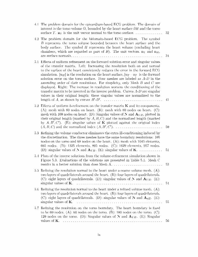
4.1 The problem domain for the epicardium-based ECG problem. The domain of interest is the torso volume Q, bounded by the heart surface dH and the torso surface T . nT is the unit vector normal to the torso surface................................... 32
4.2 The problem domain for the bidomain-based ECG problem. The symbol B represents the torso volume bounded between the heart surface and the body surface. The symbol H represents the heart volume (excluding heart chambers, which are regarded as part o f B ). The unit vectors, nT and n H,are surface normals................................................................................................................ 34
5.1 Effects of uniform refinement on the forward solution error and singular values o f the transfer matrix. Left: Increasing the resolution both on and normal to the surface o f the heart consistently reduces the error in the forward ECG simulation. |uH| is the resolution on the heart surface, |UT — uT | is the forward solution error on the torso surface. Four meshes are labeled as A -D in the ascending order o f their resolutions. For simplicity, only Mesh B and C are displayed. Right: The increase in resolution worsens the conditioning o f the transfer matrix to be inverted in the inverse problem. Curves A -D are singular values in their original length; these singular values are normalized to thelength o f A, as shown by curves B '-D '........................................................................... 41
5.2 Effects o f uniform h-refinement on the transfer matrix K and its components.(A ): mesh with 60 nodes on heart. (B): mesh with 80 nodes on heart. (C): mesh with 100 nodes on heart. (D): Singular values of N and A , plotted in their original length (marked by A, B, C ) and the normalized length (marked by A, B ',C '). (E): singular values o f K plotted against the original index(A, B , C ) and the normalized index (A, B ', C ') ............................................................ 50
5.3 Refining the volume conductor eliminates the extra ill-conditioning induced by the discretization. The three meshes have the same boundary resolutions: 105 nodes on the torso and 60 nodes on the heart. (A ): mesh with 1045 elements,665 nodes. (B): 1325 elements, 805 nodes. (C ): 1629 elements, 957 nodes.(D): singular values of N and A . (E): singular values o f K ............................... 51
5.4 Plots o f the inverse solutions from the volume-refinement simulation shown in Figure 5.3. Evaluations o f the solutions are presented in Table 5.1. Mesh C results in a better solution than does Mesh A .............................................................. 53
5.5 Refining the resolution normal to the heart under a coarse volume mesh. (A): two layers of quadrilaterals around the heart. (B): four layers of quadrilaterals.(C): eight layers o f quadrilaterals. (D): singular values of N and A . (E): singular values o f K . ........................................................................................................ 54
5.6 Refining the resolution normal to the heart under a refined volume mesh. (A): two layers of quadrilaterals around the heart. (B): four layers of quadrilaterals.(C): eight layers o f quadrilaterals. (D): singular values of N and A vH. (E): singular values o f K . ........................................................................................................ 55
5.7 Refining the resolution on the torso boundary. The heart boundary is fixed to be 60 nodes. (A ): 60 nodes on the torso. (B): 100 nodes on the torso. (C):120 nodes on the torso. (D): Singular values of N and A . (E): Singular values of K . ......................................................................................................................... 56
ix

5.8 Refining the volume conductor of a 2D homogeneous torso slice. All three meshes share the same boundary resolution: 105 nodes on the torso and 60 nodes on the heart. (A ): mesh containing 943 elements, 584 nodes. (B): mesh containing 1297 elements, 761 nodes. (C ): mesh containing 1899 elements,1062 nodes. (D ): singular values o f N and A VH. (E): singular values o f K . . . 57
5.9 Inverse solutions of epicardial potentials corresponding to Figure 5.8 and Table 5.2. Mesh C yields a better solution than Mesh A. .................................... 59
5.10 Refining the resolution normal to the heart under a coarse volume mesh. (A ): one layer o f quadrilaterals around the heart. (B ): two layers o f quadrilaterals.(C ): four layers o f quadrilaterals. (D ): singular values o f N and A VH. (E): singular values of K . ........................................................................................................ 59
5.11 The torso mesh with heterogeneous, anisotropic conductivity. Tissue conductivity values are listed in Table 5.3. .............................................................................. 60
5.12 Effects o f refining different regions in the heterogeneous torso mesh while fixing the fidelity o f the heart boundary. (A ): the original mesh. (B ): refining the lungs. (C ): refining skeletal muscles and torso surface. (D ): combining of Band C. (E): singular values of N and A VH. (F): singular values o f K ................. 61
5.13 Refining the resolution normal to the heart. (A ): one layer o f quadrilaterals around the heart. (B): two layers o f quadrilaterals. (C): four layers of quadrilaterals. (D): singular values of N and A VH. (E): singular values o f K . 62
5.14 Singular values of the transfer matrices resulting from the sphere/torso model.The torso mesh remains unchanged while three sphere meshes are tested. N h denotes the number of nodes on the surface of each sphere. ............................... 67
5.15 Fixing the boundary discretization and refining the torso volume conductor.N e denotes the number o f elements in each mesh. (A ): singular values of A v h . (B ): singular values o f K ........................................................................................ 68
5.16 Epicardial potentials calculated from the meshes discussed in Figure 5.15, under 30-dB white noise. N e denotes the number of elements in each mesh.To effectively visualize the difference in potential patterns, the view is changed at each instant. The epicardial potentials at 21 ms exhibit the most diverse spatial pattern in the entire cardiac cycle, and hence are the hardest to recover. 69
5.17 Activation isochrones derived from reconstructed epicardial potentials in Figure 5.16. Top row: the anterior view. Bottom row: the posterior view............... 70
5.18 (A ): a cross section of the torso mesh, where the heart is surrounded by 2 layers o f prism elements. (B): the hybrid mesh at the heart-volume interface. . 70
5.19 Refining the resolution normal to the heart by prismatic elements. (A ): singular values o f A VH. (B): singular values o f K ...................................................... 71
5.20 Activation times derived from epicardial potentials calculated from the meshes in Figure 5.19. (A ): from measured potentials. (B): from the pure tetrahedral mesh. (C ): from the hybrid mesh with 1 layer o f 10-mm-thick prisms. (D): from the hybrid mesh with 2 layers o f 5-mm-thick prisms. (E): from the hybrid mesh with 4 layers of 2.5-mm-thick prisms................................................................... 72
x

5.21 Epicardial potentials computed from hybrid meshes. (A ): exact value. (B): pure tetrahedral mesh. (C ): hybrid mesh with 1 layer o f prisms. (D ): hybrid mesh with 2 layers o f prisms. (E): hybrid mesh with 4 layers o f prisms. rgrad is the ratio o f the computed value to the real value o f ||VuH ||, the L 2 norm ofthe epicardial potential gradient field.............................................................................. 72
5.22 Refining the volume while fixing the meshes around the heart by two layers o f 5-mm-thick prisms. Mesh 1, 2, and 3 contain 8106, 13636, and 23361 tetrahedral elements. (A ): singular values o f N and A . (B ): singular valueso f K ............................................................................................................................................ 73
5.23 Illustration of triangular finite elements using third-order modal expansions in the torso volume while keeping first-order (linear) expansions on the torso and heart boundaries. The modal basis expansions are illustrated in Figure 2.8.The red nodes denote the vertex modes (the element-wise linear component).The blue nodes denote the edge modes, and the green nodes denote the face m odes......................................................................................................................................... 76
5.24 The setup o f high-order finite element simulation. (A ): the two-dimensional torso mesh consists o f 1071 triangle elements with 60 nodes on the heartboundary and 105 nodes on the torso boundary. (B ): the ground truth of epicardial potentials plotted against the heart-boundary nodes. (C ): the potential field (forward solution) due to the boundary condition shown by Panel B .................................................................................................................................................. 79
5.25 Refinement using first-order (P = 1), second-order (P = 2), and third-order (P = 3) finite elements, while keeping linear approximation on the heart and torso boundaries. (A ): singular values o f the resulting transfer matrix K . (B): the relative error (RE) and the correlation coefficient (CC) o f the inverse solutions calculated under two levels o f input noise (on torso-surface potentials).(C ): the reconstructed epicardial potentials under 20 dB input noise.................. 80
5.26 Epicardial potentials calculated under 30-dB SNR input Gaussian noise. ZOT,FO T, and SOT denote the zero-, first-, and second-order Tikhonov regularization. To better show spatial patterns, the view is slightly rotated................... 86
5.27 L-curves of the norm of the solution versus the residual error when the zero- order Tikhonov is performed. The inverse problem is discretized in two scales.Mesh 1 has 27,361 tetrahedral elements with 670 triangular elements on the heart surface. Mesh 2 has 60,617 volume elements with 2,680 triangles on the heart surface. Panel A: the regularizer is the identity matrix, with the residual error and the regularizer evaluated by the Euclidean norm. Panel B: the variational regularizer derived from the mass matrix given by Table 5.4, evaluated by the continuous L 2 norm. The A value indicates the regularizationparameter corresponding to the corner of L-curves.................................................... 88
5.28 Epicardial potentials reconstructed under 30-dB SNR input noise by the zero- order Tikhonov using the traditional and the variational regularizers, corresponding to the L-curves in Figure 5.27. For each inverse solution, the relative error (RE) and correlation coefficient (CC) are given................................................ 89
6.1 Simulation setup. (A ): the animal experiment. (B): the heart/torso geometry.(C): fiber structure of a 1cm-thick slice o f the heart. (D): a cross-section of the heart mesh........................................................................................................................107
xi

6.2 Inverse solutions based on Mesh 1 with synthetic ischemia data. Results are compared between the Tikhonov and the total variation methods. Ischemic regions are indicated by the blue color. All the calculated TM Ps are in the same color scale. This figure is to be compared with Table 6.3..............................109
6.3 Inverse solutions based on Mesh 2 and Mesh 3, with synthetic ischemia data. Tikhonov and total variation solutions are presented. Ischemic regions are denoted by the blue region. All the calculated TM Ps are in the same color scale. This figure is to be compared with Figure 6.2 and Table 6.3. The mesh profiles are given in Table 6.1. ..................................................................................... 110
6.4 Inverse solutions based on Mesh 1, with clinical ischemia data. Each figure shows reconstructed heart potentials at the same cross section. The figures in each column are in the same color scale. This figure is to be compared with Table 6.4 and Table 6.5....................................................................................................... 114
6.5 Tikhonov and total variation inverse solutions based on Mesh 2 and Mesh3, using clinical ischemia data. The reconstructed heart potentials in each column are in the same color scale. This figure is to be compared with Table 6.4and Table 6.5. .................................................................................................................... 115
6.6 Inverse solutions o f an isotropic inverse model following an anisotropic forward simulation. Here Mesh 1 is being used. The reconstructed heart potentials in each column are in the same color scale. This figure is to be compared with Table 6.6 and Table 6.7....................................................................................................... 117
6.7 Inverse solutions of the isotropic heart model following an anisotropic forward simulation, based on Mesh 2 and Mesh 3. Tikhonov and total variation methods are compared under three input noise levels. The reconstructed heart potentials in each column are in the same color scale. This figure is
to be compared with Table 6.6 and Table 6.7.............................................................. 118
xii

LIST OF TABLES
1.1 Abbreviations used in this dissertation........................................................................... 6
1.2 Mathematical notations used in this dissertation........................................................ 6
5.1 Evaluation o f inverse solutions o f the annulus simulation shown in Figure 5.3. 52
5.2 Evaluation of inverse solutions o f the homogeneous torso simulation shown in Figure 5.8. ............................................................................................................................ 58
5.3 Tissue conductivities. Unit: Siemens/meter................................................................. 60
5.4 The choice o f L for Tikhonov Regularization. .......................................................... 83
6.1 Mesh configuration................................................................................................................ 107
6.2 Conductivities o f healthy heart tissues. Unit: Siemens/meter................................108
6.3 Inverse simulation with an isotropic heart model and synthetic ischemia data, over three meshes and noise levels. .............................................................................. 111
6.4 The Tikhonov inverse solutions with the anisotropic heart model and clinical ischemia data. Inverse simulation was performed over three meshes and input noise levels............................................................................................................................... 113
6.5 The total variation inverse solutions with the anisotropic heart model and clinical ischemia data. Inverse simulation was performed over three meshes
and input noise levels........................................................................................................... 113
6.6 Inverse solutions from the isotropic inverse model, with the input body-surface data coming from the anisotropic forward model. The Tikhonov method is being used here....................................................................................................................... 116
6.7 Inverse solutions from the isotropic inverse model preceded by an anisotropic forward simulation. The total variation method is performed over three meshes
and input noise levels........................................................................................................... 116

ACKNOWLEDGEMENTS
One o f the joys at the completion of my PhD journey is to acknowledge all the people
who helped and supported me along this long but fulfilling road. It was a little coincidence,
but my greatest fortune, to work with my two mentors, Dr. Chris Johnson and Dr. Mike
Kirby. W hile looking for research topics in April 2006, I was impressed and inspired by the
seminars held by the Scientific Computing and Imaging (SC I) institute, so I wrote to its
director, Chris, inquiring about research opportunities. Though never meeting me before,
Chris kindly offered me a project on electrocardiography co-advised by Mike, thus starting
my PhD journey. I am deeply grateful to both mentors for their generous guidance, support,
and encouragement throughout my graduate career. Mike's dedication to work, enthusiasm
for research, and immense knowledge set an ideal example o f academic excellence for me
to follow. As the director, Chris makes the SCI institute as close to “the ivory tower of
academia” as I idealized— I took great pleasure to work in such a supportive environment
that encourages open collaboration, intellectual freedom, and influential innovation. I
sincerely appreciate my great fortune to work with Chris side by side— His exceptional
vision, insight, finesse, and wisdom benefited not only my academic career but my whole
life.
Another professor to whom I would like to express my special gratitude is Dr. Rob
MacLeod, who kindly adopted me into his cardiac research group. Our collaboration formed
the foundation o f this dissertation. R ob has always been an invaluable mentor in many
aspects of my graduate life, including research, teaching, career guidance, academic insights,
and particularly writing and presentation. I appreciate the time and effort he has invested
in nurturing his graduate students and I feel lucky to be one o f them. He has my earnest
admiration and respect.
My PhD journey has benefited from numerous professors and colleagues whom I would
like to gratefully acknowledge. I wish to thank my external committee member, Dr. Dana
Brooks from Northeastern University, for his frequent feedback on my work, his generous
sharing of academic news, and his endless humor. I enjoyed every discussion with Dr. Sarang
Joshi, who profoundly refreshed my understanding o f mathematics. I am grateful to Dr.

Ross Whitaker for his critical but inspiring comments on my work. My former colleague, Dr.
Jeroen Stinstra, had been an essential reference point when it came to bioelectric simulation
and the development of the SCIRun software. After he left, Ayla Khan took over his role. I
deeply appreciate the support from both o f them. In addition, I am highly indebted to the
professional staff at the SCI Institute and at the School of Computing: Nathan Galli, for
polishing my posters and teaching me how to use A dobe design tools; Chems Touati, for
converting my research into multimedia; Ed Cask and Deb Zemek, for their administrative
support; and Karen Feinauer, for her kind care o f all computer science graduate students.
Numerous fellow students and friends have made my years at Utah more productive
and memorable. I appreciate my academic brotherhood with R ob M acLeod's student team:
Kedar Aras, Darrell Swenson, Brett Burton, Joshua Blauer, and Jess Tate— our numerous
lunch conversations, scientific discussions, sharing o f presentation slides, and gathering of
practice talks are enjoyable highlights o f my graduate student years. This dissertation would
not have become reality had it not been for the laborious experimental work conducted by
Kedar and Darrell. Through all these years, my close friend Fangxiang Jiao and I witnessed
each other’s growth, as we had been working under the same supervisor in the same office. I
will long remember our countless late-night working marathons, brain-storming discussions,
and our mutual encouragement. I would like to thank my fellow students, Xiang Hao, Bo
Wang, Jianrong Shu, Ran Tao, and Jingwei Zhang for the joy they brought me during my
graduate years. Special thanks to Prof. Xiaoming Sheng and his wife, Shuying Shen, who
helped me to settle down in Utah and hosted me for countless dinners on holidays. Their
hospitality brought me the warmth o f home during the past seven years.
This work is supported in part by the N IH /N C R R Center for Integrative Biomedical
Computing (Grant 2P41 RR0112553-12), and by the NSF Career Award to Dr. Mike Kirby
(NSF-CCF0347791). I also acknowledge the Treadwell Foundation and the Cardiovascular
Research and Training Institute at the University o f Utah for their support in acquiring the
experimental data.
Last, I undoubtedly owe my largest debt o f gratitude to my parents, Mr. Wang Haicheng
and Mrs. M ao Zhiyun (in Chinese convention the wife does not adopt the husband’s family
name). It is due to their unconditional love and constant support throughout my life that
I stand where I am today. Mom and Dad, I dedicate this dissertation to you.
xv

CHAPTER 1
INTRODUCTION
At a philosophical level of causality, many problems in science and engineering can
be categorized into two paradigms: forward problems and inverse problems. A forward
problem refers to understanding a physical system and predicting its behavior from some
known causes. An inverse problem consists o f determining causes that will result in a desired
or observed effect, assuming the cause-effect relation is known. Inverse problems have wide
applications in science and engineering, with motivations ranging from optimal control to
estimating inaccessible quantities from indirect observations. M y dissertation investigates
the inverse problems arising from electrocardiography.
Electrocardiography (ECG ) aims to noninvasively estimate the electrophysiological ac
tivity of the heart by measuring its resulting potential field at the body surface. Because
of recent advances in computational modeling, computing power, and imaging technology,
ECG is evolving from a basic clinical tool that relies on human interpretation to a new era of
personalized healthcare, an era in which computer models integrate not only unprecedented
complexity and realism but also biophysical information specific to individual subjects [99].
Subject-specific computer models, typically in anatomical or physical aspects, are poised to
promote mechanistic and functional studies at various biological levels ranging from cells up
to organs, opening promising opportunities for clinical diagnosis [18, 19, 17], intervention
planning, and therapy delivery [56, 35, 36, 58]. Essential to this emerging research paradigm
is the development of computational methods that leverage modern computing power to
harness quantitative models in ever-increasing complexity.
The mathematical foundation of ECG is an inverse source problem governed by partial
differential equations (PDEs) which describe the bioelectric relation between heart activities
(regarded as the source) and the body-surface potentials. Inverse problems involving PDEs
are typically challenging both mathematically and computationally: mathematically, they
are inherently ill-posed in that their solutions are either nonexistent, nonunique, or highly
unstable; computationally, they require solving large-scale numerical systems over many

2
iterations. In biomedical disciplines such as the ECG, the complexity o f biological systems
is such that their simulation taxes even the most advanced computing power and software
today. These fundamental challenges need to be overcome in order to attain solutions that
are sufficiently accurate, reliable, and efficient for clinical practice.
The overarching theme o f this dissertation is the computational formulation, optimiza
tion, and solution o f the inverse ECG problem based on finite element methods (FEMs).
This dissertation considers two types o f inverse ECG problems, hereafter referred to as
the epicardium-based inverse ECG problem and the bidomain-based inverse ECG problem,
according to how the cardiac bioelectric source is modeled. The former type has been
extensively studied whereas the latter is relatively new.
1.1 Thesis StatementThis dissertation comprises two main research thrusts: optimal discretization o f the
inverse problem, and a new inverse solution methodology called PDE-constrained optimiza
tion. Each thrust contains two major goals, leading to four thesis goals stated as follows:
1 .1 .1 G o a l 1: F in it e E le m e n t D is c r e t iz a t io n S t r a te g y
To investigate the impact o f discretization on the solution o f the epicardium-based inverse
ECG problem, and to design finite element refinement strategies specifically targeting the
inverse problem.
Successful simulation requires sensible numerical discretization of model equations. Most
existing finite-element refinement strategies, designed for forward problems, may become
inappropriate for the corresponding inverse problems by worsening their ill-conditioning.
Therefore, there is a need to develop discretization that optimizes the approximation ac
curacy o f the inverse problem while mitigating its ill-conditioning. The rationale o f the
proposed study is that a sensible discretization will improve the conditioning o f the numer
ical inverse problem, which in turn will improve the inverse solutions. Such improvement,
fulfilled during the “problem-formulation” stage, can be combined with many existing
“inverse-problem-solving” methods so as to achieve extra improvement o f the inverse so
lutions. The proposed study is two-pronged in theory and practice. The theoretical
facet comprises o f a Fourier analysis that quantifies how discretization is related to the
inverse problem's conditioning. The practical facet involves numerical simulation o f various
refinement scenarios in both two- and three-dimensional space.
Completion o f the proposed goal will result in a set of written guidelines for refining the
finite element discretization of the inverse ECG problem. The simulation experiments in

3
both two and three dimensions will verify the feasibility o f improving the inverse solution
by judicious refinements.
1 .1 .2 G o a l 2: A d a p t a t io n o f h/p- t y p e F in it e E le m e n t R e f in e m e n t
To fulfill the discretization guidelines proposed in Goal 1 by adapting spatial (h-type)
and high-order (p-type) finite element refinements.
There are two basic types o f finite element refinement. The h-type spatially refines
the mesh, whereas the p-type fixes the mesh but uses higher-order basis polynomials in
each element. Both types o f refinement need adaptation in order to fulfill a so-called
“selective refinement” required by our refinement guidelines: refining an element while
fixing the resolution at some boundaries o f this element. For the h-refinement, we use
hybrid-shaped elements involving triangular/quadrilateral elements in two dimensions and
tetrahedral/prismatic elements in three dimensions, so as to overcome the aspect-ratio
problem confronting pure triangular or tetrahedral meshes. For the p-refinement, wherever
a low-order approximation is needed, we extract the element-wise linear component and
discard all high-order components.
Completion o f the proposed goal will result in the development o f two methods that
fulfill our refinement strategies. The efficacy o f both methods will be verified via numerical
simulation experiments.
1 .1 .3 G o a l 3: In v e r s e S o lu t io n b y P D E -C o n s t r a in e d O p t im iz a t io n
To solve inverse E C G problems within a framework o f PDE-constrained optimization
that allows general form s o f objective functionals and constraints; to formulate finite element
discretization o f this framework; and to fulfill the subsequent numerical optimization using
algorithms tailored to the optimization problem ’s specific algebraic structure.
Inverse ECG problems are conventionally solved as follows: one derives (from the
physical model) and then “inverts” a transfer matrix that relates the control variables
to the observed data. The limitation o f this approach is that constraints are allowed
only on the control variables and the observed variables, and therefore, the approach may
become incompetent for optimizing complex PDE models. In contrast, the PDE-constrained
optimization incorporates the whole PDE model as a constraint, and thereby offers greater
flexibility for applying constraints. The PDE-constrained optimization currently used in
ECG problems is limited to quadratic objectives and equality constraints. We propose
a general optimization framework that enables convex objectives and constraints in both
equality and inequality forms.

4
Completion of the proposed goal will result in the development of a PDE-constrained
optimization framework that features the following ingredients: (1) deriving optimality
conditions in the continuous space, (2) closed-form finite element solutions for both the L 2-
norm minimization and the L i-norm total variation minimization, (3) inclusion of inequality
constraints, and (4) numerical optimization fulfilled by a primal-dual interior-point method
presented in a block-matrix form, tailored to the given optimization problem's specific
algebraic structure.
1 .1 .4 G o a l 4 : L o c a l iz a t io n o f M y o c a r d ia l I s c h e m ia
To use the optimization methodology proposed in Goal 3 to solve the bidomain-based in
verse ECG problem o f estimating the transmembrane potential throughout the myocardium.
To use the estimation to localize myocardial ischemia.
Traditional ECG diagnosis of myocardial ischemia, relying on human interpretation of
the body-surface signals, has limited ability to localize ischemic regions. As myocardial
ischemia can be characterized by the transmembrane potentials (TM Ps), reconstructing
a whole-heart TM P map will promote the determination of the location and extent of
ischemia. Research on the TM P reconstruction has been limited to 2D synthetic heart
models because of the problem's ill-posedness. Our new methodology of PDE-constrained
optimization will advance this research to 3D heart models with real ischemia data.
Completion of the proposed goal will result in a computer simulation study using a
realistic heart model that combines anatomical geometry, fiber structure, and experimental
ischemia voltage data. The ischemia experiment involves inducing controlled ischemia to a
live canine heart, and recording its voltages at the heart surface and within the myocardial
wall.
1.2 ContributionsThis dissertation achieves the following major contributions.
1. A systematic investigation of finite element discretization strategies specifically tar
geting the inverse ECG problem, fulfilled by (1) an h-refinement using hybrid finite
elements and (2) an adapted p-refinement (Chapter 5). This work has resulted in two
journal publications as follows:
• Wang, Kirby, and Johnson (2010). “Resolution strategies for the finite-element-
based solution o f the ECG inverse problem.” IEEE Transactions on Biomedical
Engineering, volume 57 (2): pp 220-237.

5
• Wang, Kirby, and Johnson (2011). “Finite-element-based discretization and
regularization strategies for 3D inverse electrocardiography.” IEEE Transactions
on Biomedical Engineering, volume 58 (6): 1827-1838.
2. Introducing a general PDE-constrained optimization framework to the field of inverse
ECG problems, and applying this new methodology to advance the research on
myocardial ischemia localization (Chapter 6). This work has resulted in the following
publication:
• Wang, Kirby, MacLeod and Johnson (2012). “Inverse electrocardiographic source
localization o f ischemia: an optimization framework and finite element solution.”
Journal o f Computational Physics, under review.
1.3 OrganizationChapter 2 provides the mathematical and biophysical background knowledge relevant
to the work presented in this dissertation. Chapter 3 reviews the relevant research. Chap
ter 4 describes the mathematical formulation o f the two types o f inverse ECG problems
investigated in this dissertation. Chapter 5 presents our first research thrust, the optimal
discretization (Thesis Goal 1 and 2). Chapter 6 presents our second main thrust, the
PDE-optimization for the bidomain-based inverse problem (Thesis Goal 3 and 4).
1.4 Notation and AbbreviationWe briefly describe the abbreviation and mathematical notation used in this dissertation
in Table 1.1 and Table 1.2. The general rules o f notation are as follows. A regular lower-case
letter denotes a variable or a continuous function, and a boldface lower-case letter denotes
a vector. Different fonts for the same letter usually mean the continuous or discrete version
of the same physical quantity. For example, u denotes a continuous potential field, and its
discrete version (obtained through numerical approximation) is denoted by a real vector
u £ Rn . An upper-case calligraphic letter represents a continuous functional or an operator
operating on a continuous function, e.g., Q in the expression Qu. A bold capital letter
denotes a matrix and is the discrete version o f the operator given by the same letter, if the
letter exists. For example, Q is the discrete version of Q.

6
T ab le 1.1: Abbreviations used in this dissertation.
Term Full Name Term Full NameBE Boundary Element BEM Boundary Element MethodECG Electrocardiography EXP Extracellular PotentialFE Finite Element FEM Finite Element MethodODE Ordinary Differential Equation PDE Partial Differential EquationRE Relative Error CC Correlation CoefficientTM P Transmembrane Potential TV Total Variation
T ab le 1.2: Mathematical notations used in this dissertation.
Symbol Meaning Additional ExplanationR The set o f real numberx The Euclidean coordinates in
R 2 or R 3.u, u Extracellular potential A regular lower-case letter denotes a continuum
quantity.The bold font denotes the discrete version o f the same quantity.
v, v Transmembrane potentiala Tissue conductivityHk (Q) The Sobolev space of kth-
order weak derivatives.A The stiffness matrix A bold upper letter denotes a matrix.& ^ Basis functions in finite ele
ment methodsL, L The Lagrange functional An upper-case calligraphic letter denotes a func
tional or operator in the continuous space. The bold font o f the same letter denotes the discrete matrix version of the functional/operator.

CHAPTER 2
BACKGROUND
This chapter presents background materials relevant to the research work described in
this dissertation.
2.1 Bioelectric Background2 .1 .1 C a r d ia c E le c t r o p h y s io lo g y
The mechanical action of the heart is triggered and regulated by the electrical activity of
cardiac cells originating from ionic currents. Subject to the biological activity o f cells, the
ionic currents may flow between cells or flow between the inside and outside o f a cell across
its membrane, generating a varying electric field that propagates throughout the body and
is measurable at the body surface. This mechanism forms the bioelectric foundation of
electrocardiography.
The electrical behavior o f a myocardial cell, also called a myocyte, can be characterized
by its transmembrane potential (T M P ), defined as the voltage difference between the poten
tial inside the cell (intracellular potential) and the potential outside the cell (extracellular
potential). Myocardial cells at rest maintain a stable TM P ranging from -90 to -60 mV. Once
a myocardial cell is activated, either by an intrinsic or external stimulus, its TM P will rapidly
change following a characteristic, cell-type-specific trajectory called an action potential, as
shown in Figure 2.1. Action potentials reflect the movements o f ions (N a + ,K + ,C a 2+)
through the voltage-gated ion channels embedded in cell membranes. Such movements also
cause myocytes to contract, and the propagation o f action potentials coordinates the heart
to contract efficiently as a whole, thereby demonstrating the close relationship between
mechanical and electrical activities o f the heart. Figure 2.2 shows major cardiac cell types
and their action potentials during one heart beat.
The electrical currents generated by the heart flow through the human torso, which
acts as a passive volume conductor, producing measurable body-surface potentials, known
as the electrocardiogram or ECG. Figure 2.2 shows a schematic ECG tracing and its

8
F igu re 2.1: A schematic plot o f the action potential o f a ventricular cell. Each period o f the action potential consists o f five phases: the rest phase (Phase 4), the depolarization (Phase 0), the early repolarization (Phase 1), the plateau phase (Phase 2), and the repolarization (Phase 3). The directions o f ion flows are marked with respect to the cell. This figure is adapted from the Wikimedia Commons file “File:Action potential ventr myocyte.gif” , available at http://en.wikipedia.org/wiki/Cardiac_action_potential.
temporal relationship with cardiac action potentials. A typical ECG tracing in one cardiac
cycle consists of five deflections, denoted by P, Q , R, S, and T. The P-wave reflects the
depolarization of the atria. The Q RS complex reflects the rapid depolarization of both
ventricles, followed by the ST segment which correspond to the plateau phase in action
potentials. The T wave represents the repolarization of the ventricles. The interval from the
beginning of the Q RS complex to the apex of the T wave is termed the absolute refractory
period, during which the heart is believed to be irresponsive to extra stimuli [2].
2 .1 .2 B io e le c t r i c M o d e ls in E le c t r o c a r d io g r a p h y
The bioelectric phenomena in electrocardiography are described as a “quasi-static” ap
proximation of the fundamental electromagnetic laws governed by Maxwell’s equations [42].
Because bioelectric phenomena are intrinsically of low frequencies, it has been validated
that one can safely ignore the frequency-dependent effects such as the capacitive, propa
gation, and inductive effects, as their impacts are negligible compared with the frequency-
independent portion o f the fields [42]. Therefore, although biological sources are time-
varying in a strict sense, we can make the following assumption: at each time instant, the
resulting electrical fields (currents or voltages) arise instantly to the sources, and the fields
behave as if they were in a steady state. It is under this assumption that the electrical fields

9
F igu re 2.2: Heart anatomy and electrophysiology. Schematic action potential waveforms o f cells in different parts o f the heart are shown along with the body-surface ECG signal (the bottom wave). All waveforms are temporally aligned according to their sequence of occurrence in a real heart beat. Adapted with permission from J. Malmivuo [80].
are calculated in the area o f electrocardiography— hence the term “quasi-static.”
Under the quasi-static assumption, the potential field u in a volume conductor Q is
described by the Poisson’s equation described as follows:
V - (ff(x )V u (x )) = — Isv(x ), x e Q, (2.1)
where a is the conductivity tensor measured in “Siemens/meter.” The right side term, Isv,
denotes the current source measured in “A m pere/m 3,” and is normally represented by a
physiologically-based source model.
2 .1 .2 .1 T o r s o C o n d u c t io n M o d e l
Let B denote the torso volume between the heart surface and the body surface. It is
considered a passive volume conductor without electrical sources, and the above Poisson’s
equation reduces to the Laplace’s equation as follows:
V ■ (a (x )V u (x )) = 0, x e B ;
n ■ a (x )V u (x ) = 0, x e dB ;
(2.2)
(2.3)

10
where n denotes the unit vector normal to the torso surface dB . The boundary condition
on the torso surface means that no electric currents leave the body into the air. This torso
model is to be coupled with some heart source model in order to simulate the body-surface
ECG.
2 .1 .2 .2 B id o m a in H e a r t M o d e l
The bidomain model is currently the best compromise between fidelity to the underlying
cellular/tissue behavior and achieving a computationally tractable approach to simulating
the electrical behavior of cardiac tissue [42, 91, 12]. It is a macroscopic model that
stems from the structure o f the myocardium (Figure 2.3), relating myocardial conductive
properties, ion currents, and membrane kinetic models. Myocardial tissue consists of
an intracellular space within each cell, and an extracellular (or interstitial) space that
surrounds cells. The bidomain model homogenizes the discrete ensemble o f individual cells,
assuming that the myocardium is composed o f one intracellular domain and one extracellular
domain, both o f which are continuums that span the entire heart volume. At every point
o f heart volume, both domains coexist, separated by the cell membrane and coupled by
transmembrane currents flowing from the intracellular space to the extracellular space.
The bidomain model involves three potential fields: the intracellular potential ui , the
extracellular potential ue, and the transmembrane potential v, all o f which are defined over
the heart volume H . In each domain, employing the volume conductor Equation (2.1), we
obtain the following equations:
F igu re 2.3: The bidomain model. (A ): the structure o f cardiac cells (myocytes). (B ): the schematic illustration of the bidomain model, adapted from [116] at courtesy o f the Cardiac Arrhythmia Research Package.
11
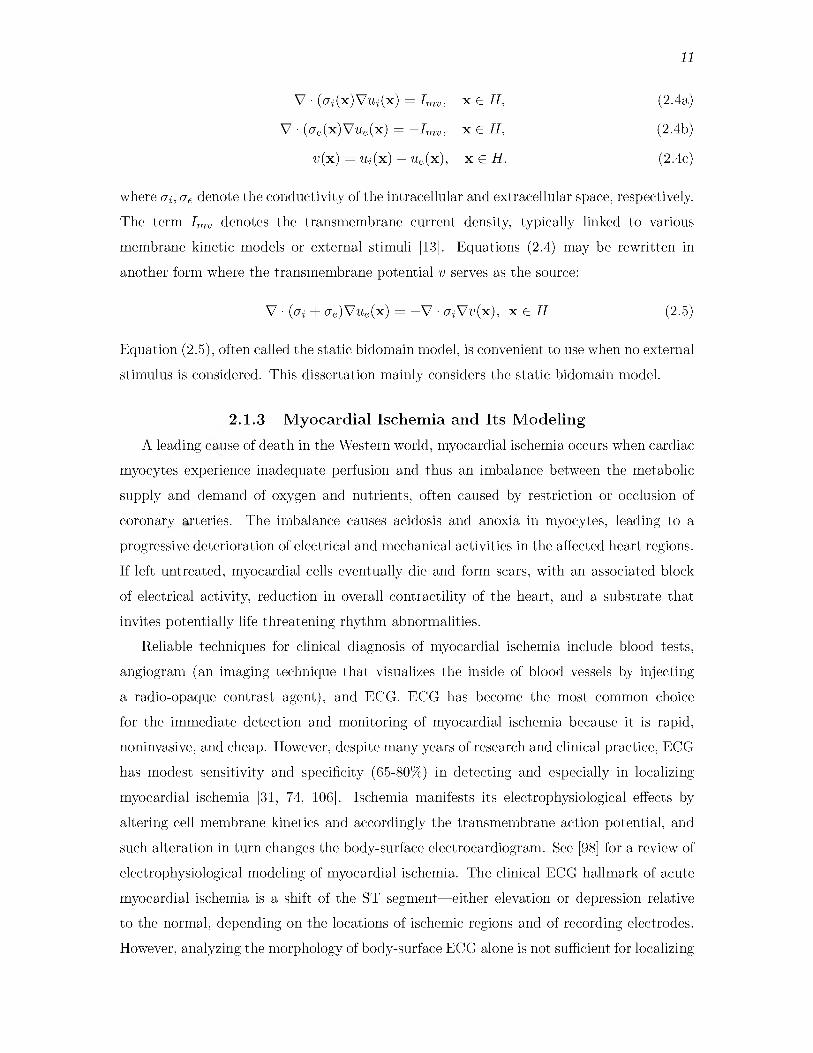
V - (a j(x )V u j(x ) = Imv, x £ H,
V - (ffe(x)VU e(x) = —Imv, X £ H,
v (x ) = Uj(x) — ue(x ), x £ H.
(2.4a)
(2.4b)
(2.4c)
where a*, ae denote the conductivity of the intracellular and extracellular space, respectively.
The term Imv denotes the transmembrane current density, typically linked to various
membrane kinetic models or external stimuli [13]. Equations (2.4) may be rewritten in
another form where the transmembrane potential v serves as the source:
Equation (2.5), often called the static bidomain model, is convenient to use when no external
stimulus is considered. This dissertation mainly considers the static bidomain model.
A leading cause o f death in the Western world, myocardial ischemia occurs when cardiac
myocytes experience inadequate perfusion and thus an imbalance between the metabolic
supply and demand o f oxygen and nutrients, often caused by restriction or occlusion of
coronary arteries. The imbalance causes acidosis and anoxia in myocytes, leading to a
progressive deterioration of electrical and mechanical activities in the affected heart regions.
If left untreated, myocardial cells eventually die and form scars, with an associated block
o f electrical activity, reduction in overall contractility o f the heart, and a substrate that
invites potentially life threatening rhythm abnormalities.
Reliable techniques for clinical diagnosis o f myocardial ischemia include blood tests,
angiogram (an imaging technique that visualizes the inside of blood vessels by injecting
a radio-opaque contrast agent), and ECG. ECG has become the most common choice
for the immediate detection and monitoring o f myocardial ischemia because it is rapid,
noninvasive, and cheap. However, despite many years o f research and clinical practice, ECG
has modest sensitivity and specificity (65-80%) in detecting and especially in localizing
myocardial ischemia [31, 74, 106]. Ischemia manifests its electrophysiological effects by
altering cell membrane kinetics and accordingly the transmembrane action potential, and
such alteration in turn changes the body-surface electrocardiogram. See [98] for a review of
electrophysiological modeling of myocardial ischemia. The clinical ECG hallmark o f acute
myocardial ischemia is a shift o f the ST segment— either elevation or depression relative
to the normal, depending on the locations of ischemic regions and o f recording electrodes.
However, analyzing the morphology of body-surface ECG alone is not sufficient for localizing
V ■ ( a + ae)V u e(x ) = —V ■ a jV v (x ), x £ H (2.5)
2 .1 .3 M y o c a r d ia l I s c h e m ia a n d Its M o d e l in g

12
ischemic regions [74, 98], so it is o f clinical interest to recover the bioelectric field within
the myocardium.
The impact of myocardial ischemia on electrocardiography has been investigated by a
number o f studies, although the mechanisms remain not fully understood [50, 74]. Figure 2.4
shows an example o f ischemic action potentials and ischemic heart potentials during the
plateau phase. During the plateau phase o f the action potential, there is normally about
200 ms o f stable and uniform TM P amplitude, resulting in equipotential conditions through
out the heart and almost no body-surface ECG signal— the isopotential ST segment of the
ECG. In ischemic cells, however, the plateau-phase TM P has lower amplitudes, forming
a voltage difference between healthy and ischemic regions. The voltage difference results
in extracardiac currents and ultimately ST-segment shifts in the body-surface potentials.
The resulting ECG patterns are temporally stable and spatially fairly simple, suggesting
that it may be feasible to reconstruct the TM P within the myocardium and to use the
reconstruction to localize ischemic regions. The bidomain heart model, in which the TM P
forms the source, provides arguably the most effective and efficient means o f simulating
myocardial ischemia and has been used extensively to investigate the relation between the
cellular origins and extracardiac (ST-segment) consequences o f ischemia [50, 74].
F igu re 2.4: Electrophysiology o f myocardial ischemia. (A ): typical action potentials o f an ischemic myocardial cell and a healthy one. (B ): extracellular potentials measured from a live ischemic canine heart at the plateau phase, shown in a longitudinal cross section view.

13
2.2 Mathematical Background2 .2 .1 G a le r k in F in it e E le m e n t M e t h o d fo r E l l ip t ic E q u a t io n s
Solving partial differential equations in realistic settings requires numerical methods such
as the finite element method (FEM ), boundary element method (BEM ), or finite difference
method (FD M ). Given that the bioelectric heart and torso models involve complex geometry
and anisotropic, heterogeneous conductivity, this dissertation adopts the finite element
method. In this section, we present formulation o f the Galerkin FEM and its treatment of
boundary conditions. The latter issue is worth discussing as the boundary conditions on the
heart surface are the goal o f inverse calculations. Boundary conditions typically represent
real physical quantities (e.g., voltage or current), and therefore, correct interpretation of
their numerical values requires the thorough understanding o f their numerical formulation.
We illustrate the Galerkin FEM using the general-form Poisson's equation with known
boundary conditions, given as follows:
R(u) = V ■ ffVw(x) + f (x) = 0 , x £ Q; (2.6)
u(x) = gD, x £ r D; a V u (x ) ■ n = gN , x £ r N ; (2.7)
where the domain Q is bounded by two boundaries: a Dirichlet-type boundary r D and a
Neumann-type boundary r N , where gD and gN are known functions. The function f (x)
denotes the source term and is also known.
The formulation of the FEM comprises two principal procedures. The first procedure
is to approximate the solution by a linear combination o f predefined functions (known as
the basis or trial functions). The second procedure is to determine the coefficient for each
trial function by enforcing certain optimization criterion, for which the Galerkin method
was adopted in this dissertation. Other common criteria include the collocation method,
the least-square method, the subdomain method and the Ritz method. Detailed discussion
o f these methods is available in [70].
In the first procedure, we decompose the exact solution u into two parts: u (x) = uD(x) +
uH (x). The function uD (x) is chosen to satisfy the Dirichlet boundary condition, whereas
the homogeneous part uH(x) is zero on the Dirichlet boundary. We approximate u by
representing uH(x) with a finite expansion in the following form:
NuH (x) « uH(x) = ^ uk (x), (x) = 0 on r D, k = 1 . . . N, (2.8)
k=lu (x) « u (x) = uD(x) + uH(x), (2.9)

14
where {^ k} are called trial functions, and {u k} are the coefficients to be determined. It is
in the construction o f the trial functions that the concept of “finite element discretization”
arises, which involves tessellating the problem domain Q and representing the trial functions
by piece-wise polynomials. A basic but common choice is the linear finite element method,
in which each trial function ^ is a piecewise linear function and accordingly, each coefficient
uk gives the value of u (x) at node k.
Substituting u into Equation (2.6), the residual R (u) is no longer zero. The coefficients
{{ik} are determined by minimizing the residual in certain ways. There is a general approach
called the weighted residual method, which requires the inner product o f the residual and
some test functions be zero:
(R (u ),^ i)n = 0, i = 1 , . . . , N ; (2.10)
where {^ i } are called the test functions, and (■, -)n denotes the Legendre inner product of
two functions in the space L 2(Q), defined as:
(g i(x ) ,g 2(x ))n = gi ■ g2 dx. (2.11)n
The Galerkin method is a special case o f the weighted residual method. In the Galerkin
method, the test functions are chosen to be the same as the trial functions, and Equation
(2.10) becomes
(R (u ),0 i)n = ( (V ■ (aV u ) + f = 0, i = 1, . . . , N ; (2.12)n
Applying the divergence theorem to Equation (2.12), we obtain
f a V u H ■ V ^ idQ = f f ^ idQ — f a V u D ■ V ^ idQ + f -dl10 i dS, i = 1 , . . . , N, (2.13)Jn Jn Jn JrN dn
where all terms on the right side are known. This equation is called the weak or variational
form o f the original Poisson’s equation.
Expanding uH according to Equation (2.8), we can write Equation (2.13) in a matrix
form as follows:
AU = F + J + D , (2.14)
where A i,j = (V 0 i , a V ^ j)n , i = 1 . . . N, j = 1 . . . N ; (2.15)
Fi = ( f , 0 i ) n , D i = (a V u D, V ^ i)n ; (2.16)/* du
Ji = - - 0 i dS, i = 1 . . . N . (2.17)./rN dn
Here the matrix A is called the stiffness matrix. The vector F represents the contribution
of the source term f , J the contribution o f the Neumann boundary condition, and D the

15
contribution o f the Dirichlet condition. The presence o f these three terms depends on the
specific conditions of the given PDE problem. The only unknown is the vector U, which
contains the coefficients { uk} , k = 1 . . . N . Solving Equation (2.14) yields the numerical
solution for the original Poisson’s Equation (2.1). Note that the stiffness matrix A is sparse,
symmetric, and positive-definite, so Equation (2.14) is amenable to iterative methods such
as the preconditioned conjugate gradient method.
2 .2 .1 .1 B o u n d a r y C o n d i t i o n E n fo r c e m e n t
Equation (2.13), the weak formulation, shows that the Neumann boundary condition is
naturally incorporated into the Galerkin formulation via direct substitution. Because the
Neumann condition is weighted by the test function 0j, the numerical solution u satisfies
the Neumann boundary condition only approximately. In contrast, u satisfies the Dirichlet
boundary condition exactly, because the Dirichlet condition is enforced independently o f the
weak formulation (which computes only the homogeneous part uH). If given in an analytic
form, the Dirichlet boundary is implemented according to Equation (2.16). In practice, the
Dirichlet condition is often given in the form of values on a discrete set o f boundary nodes.
In such a case, it is interpolated using some basis functions before being applied to Equation
(2.16), but the resulting numerical solution u still exactly satisfies the Dirichlet condition
on those boundary nodes.
2 .2 .1 .2 F in it e E le m e n t R e f in e m e n t
The finite element method calculates an approximate solution to the given PDE. The
approximation error is reduced by refining the discretization. There are two basic refinement
schemes: the h-type refinement, which spatially refines the finite element mesh, and the
p-type refinement, which keeps the mesh fixed but increases the order of basis polynomials
in each element. Refinement is typically performed based on some error estimates, and this
is called adaptive refinement.
In this dissertation, we considered mainly the linear finite element and the h-type
refinement. In the study o f the epicardium-based inverse ECG problem, we proposed an
adapted p-type refinement method.
2 .2 .2 H ig h -O r d e r F in it e E le m e n ts w ith M o d a l E x p a n s io n
The high-order finite element method, often known as the p-type refinement, keeps the
spatial mesh fixed and increases the order of basis polynomial functions within each element.
The construction o f suitable higher-order basis polynomials is also called polynomial expan

16
sion. W ith the same number of degrees o f freedom, the p-refinement usually achieves more
accurate numerical approximation than the h-refinement: for infinitely smooth solutions,
the p-refinement typically attains an exponential decay o f approximation error (with respect
to the number o f fidelities), whereas the h-refinement attains a polynomial convergence rate.
One may adopt a combined hp-refinement by both spatially refining the meshes and using
higher-order basis polynomials either uniformly or selectively in the domain.
The choice of polynomial expansion significantly influences the resulting finite element
solutions in terms o f approximation accuracy, numerical efficiency, and the conditioning
o f certain matrices resulting from finite element formulation. Numerical scientists have
proposed various types of polynomial expansions and investigated their properties exten
sively, with a comprehensive overview o f this research domain available at [70]. Generally
speaking, polynomial expansions fall into two categories: the modal expansion and the nodal
expansion. In the nodal expansion, the definition of a basis polynomial depends on a given
set o f “nodal” points spatially located within the element, e.g., the Lagrange polynomial.
In the modal expansion, the construction of basis polynomials does not depend on interior
nodal points, but rather follows certain predetermined forms.
In this dissertation, we considered a hierarchical modal expansion based on the Jacobi
polynomials, which is a commonly used modal expansion in finite element methods. In the
standard one-dimensional domain £ e [-1 ,1 ] , let 0 P (£) denote the basis functions o f order
P defined as
f (1 - 0 / 2 , p = 0;< ( £ ) = f ( ¥ ) ( ¥ ) Jp1-1i(£ ), 0 < p < P ; (2.18)
I ( 1 + £ )/2 , p = P ;
where Jp-11(£) denotes the Jacobi polynomial. Figure 2.5 illustrates the basis functions
for P = 5. Note that only the linear basis functions 0o(£) and ^s(£) are non-zero at the
boundary points, and they are called the boundary modes. The rest of the basis functions
are called interior modes as they are zero at the boundary. Also note that this expansion is
hierarchical in the sense that an expansion set of order P is built from, and encompasses,
the expansion set of order P - 1.
Based on one-dimensional (1D) basis functions, one may construct modal basis functions
in higher dimensions. For quadrilateral regions in 2D or cubic regions in 3D, the basis
functions are constructed by simply multiplying 1D basis functions along each Cartesian
dimension, as shown below:

17
-1-1
p=0
o -1
p=1
-1
p=21
" X1 / \
0/ \
0\
\-1 -1 \ J
-1-1 o 1 -1
A A1
0A A
1
0\ \ \\ J -1 \J -10 1 -1 0 1
F igu re 2.5: Examples of modal expansion functions for a polynomial order o f five as defined in Equation (2.18). The functions are normalized to the value range of [ -1 ,1 ].
$pq(Cl, ^2) = <Pp(i l ) < P q - 1 < Cl, 2 < 1; (2 .19)
where 0p, 0q are given by Equation (2.18), 0 < p < P l , 0 < q < P2. (2.20)
Figure 2.6 illustrates the construction o f 2D modal basis functions over a standard quadri
lateral region. By increasing the order Pl and P2, the basis expansion can represent higher
spatial frequencies (fluctuations) in the underlying continuum field.
An important advantage of the above modal basis functions is their inherent decom posi
tion into three modes: the vertex mode, the edge mode, and the face mode, as illustrated in
Figure 2.7. Each vertex mode is non-zero at one node. Each boundary mode has non-zero
support at one boundary and becomes zero on the rest boundaries. The face modes are
zero on all boundaries, with non-zero support only in the interior of an element. For
three-dimensional regions, the decomposition includes an extra volume mode in which the
basis functions have non-zero support only within the region volume.
Such decomposition gives rise to two desirable properties for the finite element method.
The first is the convenience for the global assembly procedure in the finite element method,
a procedure that combines the numerical systems derived from each element into a global
system. The classical Galerkin finite element approximation requires C 0 continuity on

18
F ig u re 2.6: Construction o f two-dimensional modal basis functions from the product of two one-dimensional basis functions given by Equation (2.18). The basis functions are o f the order P = 4 in each dimension. Courtesy of G. Karniadakis [70], (§2005 Oxford University Press. Reprinted by the permission o f Oxford University Press.
Edge modes
F ig u re 2.7: The modal basis functions shown in Figure 2.6 are decomposed into vertex /edge/face modes. The grid diagram illustrates where each mode is conceptually located in the element, with red nodes denoting the vertex modes, blue nodes denoting the edge modes, and green nodes denoting the face modes. Adapted from [70] courtesy o f G. Karniadakis.
interelement boundaries. This requirement is fulfilled by adjusting the vertex modes and
boundary modes between adjacent elements. The second advantage is the flexibility to
tune the order o f expansion within each individual element, both because o f the modal
design that each face mode (or volume mode in 3D) is locally defined within one element,
and because o f the hierarchical design that a high-order expansion encompasses low-order
expansions.
The modal basis functions for triangular regions in 2D or tetrahedral regions in 3D
are constructed in a similar way as elaborated in the Appendix. An extra procedure of
coordinate transformation is needed to convert the quadrilateral basis functions into the
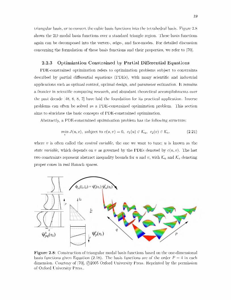
19
triangular basis, or to convert the cubic basis functions into the tetrahedral basis. Figure 2.8
shows the 2D modal basis functions over a standard triangle region. These basis functions
again can be decomposed into the vertex-, edge-, and face-modes. For detailed discussion
concerning the formulation of these basis functions and their properties, we refer to [70].
2 .2 .3 O p t im iz a t io n C o n s t r a in e d b y P a r t ia l D if fe r e n t ia l E q u a t io n s
PDE-constrained optimization refers to optimization problems subject to constraints
described by partial differential equations (PDEs), with many scientific and industrial
applications such as optimal control, optimal design, and parameter estimation. It remains
a frontier in scientific computing research, and abundant theoretical accomplishments over
the past decade [48, 6, 8, 7] have laid the foundation for its practical application. Inverse
problems can often be solved as a PDE-constrained optimization problem. This section
aims to elucidate the basic concepts of PDE-constrained optimization.
Abstractly, a PDE-constrained optimization problem has the following structure:
m in J (u, v), subject to e(u, v) = 0, c i(u ) € Ku, c2(v) € K v. (2.21)V
where v is often called the control variable, the one we want to tune; u is known as the
state variable, which depends on v as governed by the PDEs denoted by e(u, v). The last
two constraints represent abstract inequality bounds for u and v, with Ku and Kv denoting
proper cones in real Banach spaces.
F igu re 2.8: Construction o f triangular modal basis functions based on the one-dimensional basis functions given Equation (2.18). The basis functions are o f the order P = 4 in each dimension. Courtesy of [70], © 2005 Oxford University Press. Reprinted by the permission of Oxford University Press..
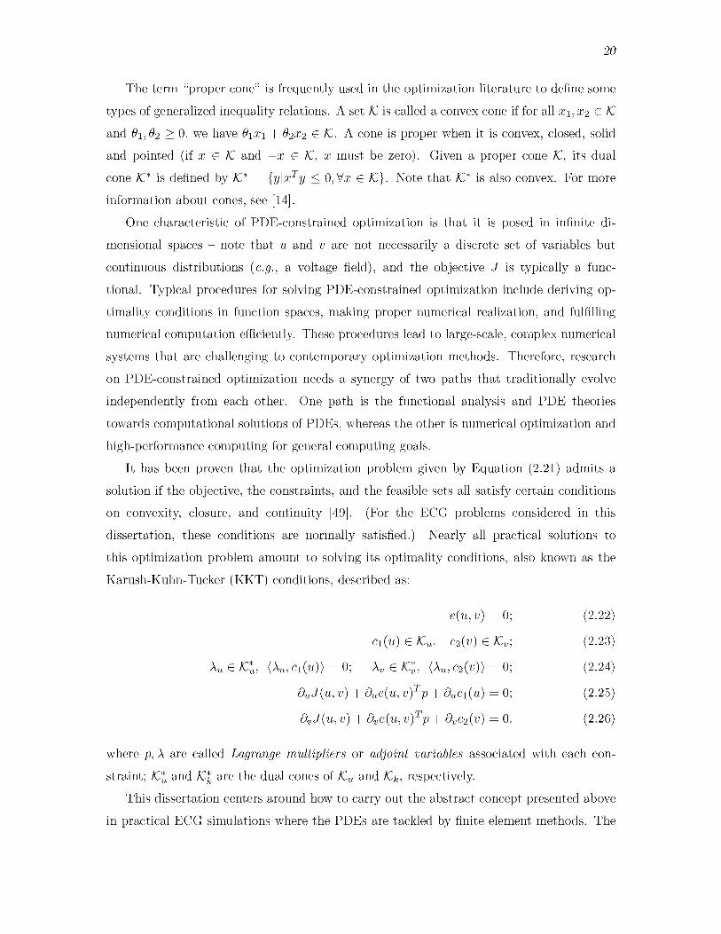
20
The term “proper cone” is frequently used in the optimization literature to define some
types o f generalized inequality relations. A set K is called a convex cone if for all x 1, x 2 e K
and d1,0 2 > 0, we have d1x 1 + d2x 2 e K. A cone is proper when it is convex, closed, solid
and pointed (if x e K and —x e K, x must be zero). Given a proper cone K, its dual
cone K* is defined by K* = {y|xTy < 0, Vx e K }. Note that K* is also convex. For more
information about cones, see [14].
One characteristic of PDE-constrained optimization is that it is posed in infinite di
mensional spaces - note that u and v are not necessarily a discrete set o f variables but
continuous distributions (e.g., a voltage field), and the objective J is typically a func
tional. Typical procedures for solving PDE-constrained optimization include deriving op
timality conditions in function spaces, making proper numerical realization, and fulfilling
numerical computation efficiently. These procedures lead to large-scale, complex numerical
systems that are challenging to contemporary optimization methods. Therefore, research
on PDE-constrained optimization needs a synergy of two paths that traditionally evolve
independently from each other. One path is the functional analysis and PDE theories
towards computational solutions of PDEs, whereas the other is numerical optimization and
high-performance computing for general computing goals.
It has been proven that the optimization problem given by Equation (2.21) admits a
solution if the objective, the constraints, and the feasible sets all satisfy certain conditions
on convexity, closure, and continuity [49]. (For the ECG problems considered in this
dissertation, these conditions are normally satisfied.) Nearly all practical solutions to
this optimization problem amount to solving its optimality conditions, also known as the
Karush-Kuhn-Tucker (K K T) conditions, described as:
where p, A are called Lagrange multipliers or adjoint variables associated with each con
straint; KU and K*k are the dual cones of K u and K k, respectively.
This dissertation centers around how to carry out the abstract concept presented above
in practical ECG simulations where the PDEs are tackled by finite element methods. The
e(u, v) = 0;
c1(u) e Ku, c2(v) e Kv;
Au e KU, (Au,C1(u)) = 0; Av e K*, (Au,c2(v)) = 0;
duJ (u, v) + due(u, v )Tp + duC1(u) = 0;
dv J (u, v) + dv e(u, v )Tp + dv C2(v) = 0.
(2.22)
(2.23)
(2.24)
(2.25)
(2.26)

21
goal is to translate the mathematical formulation into a numerical system for efficient and
robust numerical optimization.

CHAPTER 3
RELEVANT WORK
This chapter presents how the work o f this dissertation is related to previous studies
in the field of inverse problems o f electrocardiography (ECG ), and its contribution in the
aspect o f modeling, computational methodology, and clinical application.
3.1 Review of Various Forms of Inverse ECG ProblemsElectrocardiographic simulation comprises three basic components: a source model rep
resenting cardiac activities, a volume conductor model, and computational methods. In this
dissertation, the inverse ECG problem involves quantitatively identifying the parameters
o f the selected source model such that the resulting potentials at the body surface will
closely match the measured values. Hereafter, we refer to the calculated source parameters
as the inverse solution, and refer to the process o f solving an inverse problem as inverse
calculation.
The inverse ECG problem has various formulations depending on the choice o f source
models. The choice is basically a compromise between a m odel’s realism, accuracy, complex
ity, and the uniqueness o f the inverse solution for this model. Most source models in current
clinical use are based on discrete dipoles or other simplifications, which are not measurable.
In order to promote the credibility of inverse ECG solutions, it is desirable to use a source
model that not only captures the pathophysiological activities o f the heart but also enables
experimental measurement for validating the calculated solution. However, the complexity
o f such a model may make the inverse problem difficult to solve: the problem may have
nonunique solutions, or its solution may be highly unstable to input noise and modeling
inaccuracy. On the other hand, a simple source model typically results in a better-posed
inverse problem that promises an accurate solution, although the solution may offer limited
information o f heart activities.
In this section, we review recent progress on the inverse ECG problem according to
the heart source models being used, including the two most popular approaches of source

23
formulation— the epicardial potentials and the activation wavefronts. We also review less-
popular source formulations such as surface transmembrane potentials, myocardial po
tentials, and the bidomain-based models. Given the limited space o f this dissertation,
we omit simple source models such as single dipole, moving dipole, multipole series, or
fixed-location multiple dipole in view o f their relatively low biological relevance and their
difficulty o f experimental validation. Inverse solutions in terms o f these simple models have
been summarized in [42, 41], and no significant progress has been reported ever since. For
additional information, we refer the readers to [92] for a comprehensive and recent survey
of inverse ECG problems, and to [77] for a review of fundamental theories and models.
3 .1 .1 In v e r s e S o lu t io n o f E p ic a r d ia l P o te n t ia ls
The most straightforward and popular inverse ECG problem is to reconstruct the ex
tracellular potential on the epicardial surface [9]. This inverse problem is also a major
research subject of this dissertation and its formulation will be elaborated in Section 4.1.
Besides its close physiological relevance, the epicardial potential solution has the advantage
o f allowing direct validation [18, 19]. In recent years, this approach has advanced to
the level o f human clinical studies [123, 121, 122, 120, 23, 24], such as understanding
heart activation and repolarization [97]; diagnosing ventricular tachycardia [56], W P W
syndrome [34], and arrhythmia [95]; planning cardiac resynchronization therapy [58]; and
guiding catheter-based ablation for the W P W syndrome [36, 35]. W ith the heart source
acting as a Dirichlet boundary condition to the torso volume conductor, this inverse problem
is linear and admits a unique solution [125], but is severely ill-posed.
Overcoming the ill-posedness has been a primary goal of the research on the inverse epi-
cardial solution, and many regularization methods have been proposed. A popular yet basic
method is the Tikhonov regularization with a spatial constraint on epicardial potentials,
with the regularization weighting parameter being determined by several methods [45, 67].
Other basic methods that have been used include the truncated SVD method [46], the
total variation method [37], and the iterative Krylov-subspace-based GMRes method [96].
These methods share the common property that they solve the inverse problem at each time
instant independently, without considering the temporal correlation o f epicardial potentials
at adjacent time instants.
More advanced regularization methods attempt to incorporate both spatial and temporal
constraints on the solution, exploiting either the temporal correlation o f cardiac activities
or any prior knowledge about the temporal characteristic o f cardiac electrical signals. An
initial effort called Twomey regularization [89] restrains the Tikhonov solution at one

24
instant from changing too drastically from preceding ones. Later, three approaches o f joint
spatial-temporal regularization were separately proposed, hereby referred to as the multiple
regularization, the state-space model, and the isotropy model. The multiple regulariza
tion [15] approach imposes one spatial and one temporal constraint simultaneously on the
inverse solution over multiple time instants. Imposition o f multiple constraints makes the
inverse solution more robust to regularization parameters, but the computational complexity
grows significantly when more than two constraints are included. The state-space model [10]
realizes the temporal constraint by a known evolution model for the epicardial potentials
plus a random perturbation. This temporal model is coupled with the forward model (hence
the name “state-space” ), and the pair o f equations are effectively solved via a Kalman
filter algorithm. The isotropy model [39, 40] formulates the inverse problem across all
time instants. This approach, based on the “isotropy” assumption that the spatial and
temporal correlations are separable, first de-correlates the input data temporally, then
solves the inverse problem instant by instant (with regular spatial regularizations), and
finally re-correlates the inverse solutions temporally. The isotropy model has the attraction
of needing no prior knowledge about the temporal behavior o f heart potentials, but the
assumption o f isotropy (time-space separability) is not physically justified. A comparative
study showed that the above three apparently distinct approaches can be unified into the
same statistical framework but express different assumptions [126]. Finally, another multiple
spatial-temporal constraint approach was proposed based on convex optimization [3]. This
approach, instead o f minimizing an objective, simply searches a solution that satisfies
all the constraints, requiring no regularization parameter and no limit on the number of
constraints. The correctness of the solution completely relies on the appropriateness of the
applied constraints. This approach flexibly admits constraints that are less mathematically
tractable in the Tikhonov framework.
As we reviewed above, extensive achievements have been made on the inverse epicardial
solutions. However, there are still opportunities to further improve the inverse epicardial
solution in terms o f its accuracy, robustness, and applicability to various cardiac scenarios.
An important but often neglected way to improve inverse solution accuracy is to improve
the numerical formulation of the inverse problem before seeking its inverse solution. In
fact, a good numerical formulation can be built on top o f effective regularization methods
to achieve additional gains in the inverse solution accuracy. This consideration forms the
rationale that motivates our study presented in Chapter 5.

25
3 .1 .2 In v e r s e S o lu t io n o f A c t iv a t io n T im e s
Another popular inverse problem approach is to reconstruct the time of activation at
each point on the heart surface (which in this section means the union o f epicardial and
endocardial surfaces). This approach is not investigated in this dissertation. The purpose
o f presenting it here is to complete our review o f inverse ECG problems and to compare it
with our bidomain-based inverse problem.
In this approach, the heart source is represented by a layer o f dipoles uniformly dis
tributed at the activation wavefront, pointing normal to the surface from the activated
region toward the yet-to-activate region. By assuming the activation wavefront touches
both the epicardial and endocardial surfaces, the above source representation is equivalent to
dipoles located at the already-activated epicardial and endocardial surfaces. This approach
imposes a strict constraint on the source model by assuming all dipoles act as a two-phase
step function with a predetermined amplitude. Such formulation results in a nonlinear
inverse model that relates body-surface potentials to the heart-surface activation time, the
only unknown source parameter.
Because o f its restrictive parameterization o f the source model, the activation-time
inverse problem is not only much better-posed than the inverse problem o f epicardial
potentials, but is also more robust than the latter to errors in geometry and body-surface
measurements. The two approaches were compared in details in [21]. On the other hand,
the activation-time approach is limited to activation and poorly characterizes other cardiac
electrical activities. Thus, this approach is most suitable for studying rhythmic disturbances
and ectopic beats, but may not be appropriate for myocardial ischemia or infarction.
We now briefly review the major research progress in the activation-time inverse prob
lem. After its initial proposal in the 1980s [26, 25], researchers developed the Tikhonov
regularization for its inverse solution [54], and investigated the effect o f torso geometry
and heart position in this inverse approach [55]. These early studies carried out inverse
calculation by constraining the activation isochrones, based on the belief that the activation
isochrones were inherently smooth in space and therefore, regularizing them was more
effective than regularizing the heart potential field. Later, a fundamentally different method
to reconstructing activation isochrones was proposed [53, 38], based on the concept of
“critical points,” which refer to the local minima, maxima, and saddle points in the map of
heart-surface activation times. The basic procedure o f this method is to first identify the
critical points and their associated activation time, and then to use this information as a
constraint in the inverse calculation for the full activation-time solution. The key rationale

26
of this method is that each critical point happens when a propagating transmural activation
wavefront intersects the heart surface. Such intersection generates a sudden alteration in
the body-surface potential recordings. The critical points were identified by processing
body-surface potentials, for which two methods were developed: the initial one exploited
the jum p in the temporal derivative o f body-surface potentials [38] whereas the other one
applied a multiple-signal-classification algorithm on body-surface potentials [53].
3 .1 .3 In v e r s e S o lu t io n o f S u r fa c e T r a n s m e m b r a n e P o te n t ia ls
As we have described, the epicardial-potential source model possesses high flexibility
whereas the activation-based source model is strictly constrained so as to stabilize inverse
solutions. Achieving a trade-off between the two approaches motivates the use o f the heart-
surface transmembrane potential (TM P) as the source. Such source formulation enables
one to impose physiologically-based temporal constraints on the TMP, thereby extending its
applicability beyond the activation activity. This approach is not pursued in this dissertation
so we briefly describe it here.
In this approach, the TM P is related to surface extracellular potentials via the bidomain
model along with certain assumptions about the isotropy and homogeneity o f heart tissue
conduction, and the rest o f the model formulation is similar to the epicardial-potential
model. An early study o f this inverse problem employed a temporal constraint that required
that the TM P at each site be nondecreasing in time during the QRS interval [83]. Such
formulation translated the inverse problem into a convex optimization problem, which was
then solved by a standard optimization package named MOSEK. This study reported a
good recovery o f important propagation events in both normal and abnormal hearts. A
later study reported that the inverse solution o f surface TM Ps compared favorably with the
inverse solution of epicardial potentials [82].
3 .1 .4 In v e r s e S o lu t io n o f M y o c a r d ia l P o te n t ia ls
All the inverse solutions discussed earlier are defined on the heart surface, but they
are often not sufficient to reveal cardiac activities within the myocardial volume. It is of
great clinical interest, especially for localized therapy delivery, to reconstruct the electrical
potentials throughout the myocardium. This inverse problem is typically formulated based
on the bidomain heart model described in Section 2.1.2, in which the cardiac source is
represented either by the myocardial transmembrane potential (TM P) or the current density
derived from it. This inverse problem is more difficult than recovering epicardial sources,
as it is less constrained and may not have a unique solution. Research on this problem has
27
achieved limited progress, and it remains an open question to accurately reconstruct the
myocardial potential at an arbitrary time instant. This problem is a main objective o f this
dissertation and is presented in Chapter 6.
Studies on this problem have been limited. One approach [47] used a cellular automata
model based on a predefined TM P characterization, and the inverse problem became iden
tifying the initial site of activation, which was solved by minimizing the spatial-temporal
correlation between the simulated and measured body-surface potentials. This approach is
more similar to the activation-time-based approach than a potential-based one. Another
study made by the same group [75] attempted to reconstruct the current density (the gradi
ent of TM Ps) within the myocardium, with the ultimate goal of estimating the ventricular
activation times. The rationale of this approach is that the activation time o f a site can
be determined by the maximum of the site’s time course o f current density, even though
the current density itself is inaccurate. This approach essentially reconstructs a vector field
(the current density), for which there is no unique solution and it is difficult to design
a physically justified constraint. In fact, we note that this study did not report to have
obtained accurate current densities, and therefore its approach seems to be applicable only
to recovering activation times.
Some researchers attempted to reconstruct the myocardial transmembrane potentials.
An early study o f such effort [105, 104], using an anisotropic heart model, employed
the Tikhonov method for spatial regularization and the Greensite method for temporal
regularization [40]. However, this study did not achieve a meaningful reconstruction within
the myocardium, while the reconstructed TM P on the epicardial surface was close to the
results reported by the studies based on the surface TM P source model discussed in the
preceding section. Another approach [59] sought the integral o f the TM P over the ST
segment rather than at one time instant, thereby making the inverse solution more robust
to input noise but meanwhile limiting its applicability to identifying activation.
Recently, a mathematical stability analysis decomposed the inverse problem of myocar
dial TM P into two subproblems: (1) recovering the epicardial potential and (2) computing
the TM P from the epicardial potential. It reported that while the first subproblem was
severely ill-posed, the second could be made well-posed with a proper prior [16].
Regardless of model assumptions and constraints, all the studies described above used
the same methodology in their inverse calculation: they first transform the underlying phys
ical model into a transfer matrix that relates the source parameters to the measurements,
and then carry out optimization based on the transfer matrix. An alternative methodology,

28
PDE-constrained optimization, was recently introduced to ECG problems and used for
reconstructing the myocardial TM P [85]. Instead o f forming the transfer matrix, the
PDE-constrained optimization incorporates the whole physical model as a PDE constraint,
thereby offering ample flexibility for applying various physically-based constraints. The
work o f [85] was limited to quadratic objective functionals and equality-form constraints,
and its simulation was limited to 2D models and synthetic data. A major contribution
of this dissertation is to extend that inaugural work into a general convex optimization
framework, and to apply the inverse TM P solution to localizing myocardial ischemia (see
Chapter 6).
Finally, a series o f studies, specifically aimed at myocardial ischemia localization, pur
sued a low-order parameterization o f myocardial TM Ps and thus a simplified, better-posed
inverse problem. The initial study proposed a level-set framework to parameterize the
myocardial TM P by the size and location o f ischemia [76, 86], with simulations based on
a two-dimensional torso model. A later study simplified the level-set method by assuming
that ischemia has a spherical shape [100], and extended to a simple three-dimensional heart
model, but its method did not work in the case of multiple ischemic regions.
3.2 Discretization of Inverse ProblemsMathematically, the primary challenge o f most inverse problems lies in their inherent
ill-posedness in the Hadamard sense: their solutions may not exist, may be nonunique, or
may be highly unstable with perturbations in input data. Regularization, which refers to the
mathematical technique of constraining an ill-posed problem so as to convert it to a better-
posed one, is a principal topic in inverse problem research, and there is a vast literature on
regularization [110, 111, 57, 29, 72, 68]. W hen it comes to numerical simulation, it has been
discovered that discretization o f an inverse problem is one form of regularization because it
impacts the numerical conditioning o f the discretized problem, from the viewpoints of either
functional analysis [81] or Bayesian statistics [69, 73]. Therefore, a sensible discretization
can be combined with other regularization methods to achieve additional improvement in
the inverse solution.
Speaking o f the inverse ECG problem specifically, while there have been plenty o f studies
aiming at regularization during the problem-solving stage, few studies have been devoted
to improving the numerical formulation o f the inverse problem before seeking its inverse
solution. This observation motivates our research on the discretization o f the inverse ECG
problem.
In this dissertation, we considered numerical discretization in the context of the finite

29
element method (FEM ), whose adaptation is fulfilled by the “refinement” process. Adaptive
FEMs have been applied to ECG problems, though most o f such efforts were aimed at the
forward simulation rather than the inverse simulation [101, 90, 62, 64, 61]. In these studies,
refinement was based on some element-wise error estimator and tended to refine the regions
where the potential field had a high spatial gradient. One study [101] compared the efficacy
o f such spatial adaptive refinement with conventional uniform refinements in simulating
forward ECG problems, and its findings were supported by similar results reported by an
adaptive BEM study [103].
Besides the spatial refinement, the p-type refinement using high-order finite elements
has also been used in ECG problems. One study proposed both a finite element method
and a boundary element method based on cubic Hermite interpolation [93]. Another study
reported that high-order quadrilateral elements notably improved the numerical quality of
the inverse ECG solution [30]. In [66], an algebraic multilevel method was proposed for ECG
simulation which, compared with ordinary multigrid methods, achieved more automatic
refinements and better stability in the presence o f discontinuous coefficients and boundary
conditions. However, this multilevel study did not investigate the optimal discretization
specifically for the inverse epicardial solution.
The refinement methods reviewed above are mostly oriented towards the forward prob
lem. In contrast, literature on inverse-problem-oriented discretization is limited. An early
study explored how the resolution on the epicardium and on the body surface influenced
the inverse ECG solution [90]. Another study that embodied the idea of “regularization-by-
discretization” attempted to combine a spatially-adaptive FEM with local regularization for
the inverse ECG problem [60, 63]. Its basic idea was to partition the transfer matrix (the one
relating epicardial potentials to body-surface potential, derived from the FEM ) into several
submatrices, each of which corresponds to a local region o f the potential field, and then to
apply a local regularization procedure tailored to each submatrix. Finally, it is worth noting
that adaptive FEMs are currently the state-of-art techniques in solving PDE-constrained
inverse problems [8, 7], but such techniques have not made their application to ECG
problems.
A main argument proposed by this dissertation is that the discretization refinement that
is effective for the forward ECG problem may become inappropriate for its corresponding
inverse problem [118, 119]. Because of its ill-posed nature, the inverse problem requires
different discretization considerations from its corresponding forward problem. However,
there remains a notable gap in the current ECG literature concerning the impact of resolu

30
tion on finite element simulation o f the inverse problem. It still remains an open question
as to how discretization is related to the ill-posedness of the inverse ECG problem both
qualitatively and quantitatively, and accordingly, how one should carry out discretization
that optimizes the conditioning o f the numerical inverse problem whilst minimizing the
approximation error. One goal o f this dissertation is to systematically address this open
question at a practical level.
CHAPTER 4
FORMULATION OF ECG PROBLEMS
In this chapter, we present the mathematical formulation of the two types of inverse
problems investigated in this dissertation. Our scientific research on the two problems
are to be presented in Chapter 5 and Chapter 6, respectively. We separate the problem
formulation from our research contribution in order to facilitate readers’ comprehension.
4.1 Epicardium-Based Inverse ECG ProblemIn the epicardium-based ECG problem, the heart source is represented by the potentials
on the epicardium (or in general, a closed surface surrounding the heart). This epicardial
potential source acts as the internal boundary conditions to the torso volume conductor
illustrated by Equation (2.2) and Figure 4.1, yielding the complete mathematical model
described as follows:
V ■ ff(x )V u (x ) = 0, x e Q; (4.1a)
u (x ) = u0(x ), x e d H ; (4.1b)
n ■ a (x ) V u (x ) = 0, x e T, (4.1c)
where u is the potential field in the torso volume Q, which is bounded by the heart surface
d H and the torso surface T . u0(x) denotes the known epicardial potentials. a (x ) denotes
the torso conductivity, which is a symmetric, positive-definite tensor.
W ith respect to this ECG model, the forward problem is to calculate the torso potential
u given the epicardial potential u0. Its corresponding inverse problem is to reconstruct u0
based on measurements of u at the body surface. Both the forward and inverse problems
assume that domain geometry and conductivities are known and remain fixed.
4 .1 .1 F in it e E le m e n t F o r m u la t io n
This section describes the Galerkin finite element formulation for numerically calculating
the elliptic PDE problem given by Equation (4.1). The finite element discretization is
defined as follows.

32
F igu re 4.1: The problem domain for the epicardium-based ECG problem. The domain of interest is the torso volume Q, bounded by the heart surface d H and the torso surface T . nT is the unit vector normal to the torso surface.
D e fin it io n 4.1. Let Qh denote a tessellation of Q. Let { 0 } N=Ui be the global finite
element basis functions associated with this tessellation. The finite element discretization
o f u is given by u « uh = ^ N=Ui ui^i . Let u = (u i , u2, . . . , uNu)T denote the coefficient
vector.
Linear finite elements are the most common choice in practice, in which case each basis
0 i is an element-wise linear hat function associated with node i, and ui contains the voltage
values at mesh nodes. Let the nodes o f Qh be grouped into three nonintersecting sets, on
the heart surface (denoted by H ), in the torso volume (denoted by V), and on the torso
surface (denoted by T ). The basis functions {^ i } are grouped in the same way. When
high-order finite elements are used, the basis functions {^ i } are not only associated with
mesh nodes but also with virtual points within elements. However, these high-order basis
functions can be grouped in a similar way as we deal with linear elements.
Discretizing Equation (4.1) according to Definition 4.1, applying the Galerkin formula
tion, and using the test functions from the space {^ i (x ); i e V U T } , we obtain a matrix
system as follows:
( ATV A T T ) ( ut ) = ( —A T H ) u h , (4.2)
where u V = (uk )T , k e V , u H = (uk )T , k e H and uT = (uk )T , k e T denote the coefficient
vectors corresponding to each node group. The matrices are given by:

33
A v v = (V 0 j ,a V 0 k )n, j e V ,k e V ; (4.3)
A VT = (V 0 j ,a V 0 k )n, j e V , k e T ; (4.4)
A TV = (V 0 j ,o V $ k )n, j e T , k e V ; (4.5)
A t t = (V 0 j ,uV ^k )n, j e T , k e T ; (4.6)
A v h = (V 0 j , o V $ k )n, j e V , k e H; (4.7)
a t h = (V 0 j ,a V 0 k )n, j e T , k e H. (4.8)
In the expression above, (■, -)n denotes the inner product defined as:
(^, ^ )n = f 0 (x ) ■ ^ (x ) dx. (4.9)Jn
In Equation (4.2), the right side is the “forcing term” induced by the known Dirichlet
boundary conditions. The left matrix, called a stiffness matrix, is symmetric and positive-
definite, so the solution o f this linear system is amenable to iterative methods such as the
preconditioned conjugate gradient method.
Based on Equation (4.2), we can further derive the explicit relation between the torso
potential uy and the epicardial potential uh . Normally, no elements span from the heart
to the torso surface, so A TH = 0. Also note that A v v is the stiffness matrix resulting from
the finite element solution to a zero-Dirichlet boundary condition Laplace problem and is
hence invertible. Exploiting these facts, we obtain the following relation:
u T = K u H, K = M -1 N ; (4.10)
M = A t t - A y v A - V A v t ; (4.11)
N = A y v A -V A v h . (4.12)
Here K is often named the transfer matrix, as it “transfers” the potential information from
the heart surface to the torso surface. The matrix M is well-conditioned and invertible, but
both N and K are severely ill-conditioned. The computational inverse problem involves
solving Equation (4.10) for u H.
4.2 Bidomain-Based ECG ProblemThe bidomain-based ECG model consists of a static bidomain heart model coupled with
a monodomain torso model, respectively described by Equation (2.5) and (2.2). The full
model is illustrated in Figure 4.2 and described below:

34
F igu re 4.2: The problem domain for the bidomain-based ECG problem. The symbol B represents the torso volume bounded between the heart surface and the body surface. The symbol H represents the heart volume (excluding heart chambers, which are regarded as part of B ). The unit vectors, nT and n u , are surface normals.
V - (ae(x) + ffj(x ))V u e(x) = —V ■ a jV v (x ), x € H ; (4.13)
V ■ at(x )V u b(x) = 0, x € B. (4.14)
Here Equation (4.13) describes the static bidomain heart where ue and u are the extra
cellular and intracellular potentials, respectively. The transmembrane potential v forms
the source term of the model. The tensors, ai and ae, represent the intracellular and
extracellular conductivity o f the myocardium, and these tensors are symmetric, positive-
definite matrices dependent upon spatial location. Equation (4.14) states that the torso is
a passive volume conductor. ub denotes the monodomain potential in the torso; at denotes
the conductivity.
The above model satisfies the following boundary conditions at the torso surface T and
the heart-torso interface d H :
(atV u b) ■ nT = 0, on T ; (4.15)
ue = ub, on d H ; (4.16)
(aeV u e) ■ n u = (atVub) ■ n u , on d H ; (4.17)
(ffiV u i) ■ n u = 0, on d H ; ui = ue + v. (4.18)
Here Equation (4.15) assumes that no current flows out o f the torso surface. Equation (4.16)
assumes the continuity o f potentials on d H . Equation (4.17) dictates the conservation of

35
electrical currents flowing across the heart boundary. Equation (4.18) means that the
intracellular current, ^ V u ^ is bounded within the heart, therefore indicating that only the
extracellular current flows into the torso, yielding Equation (4.17).
The above model and boundary conditions can be jointly expressed as a Poisson equation
given below:
—V ■ a V u (x ) = f ( x ) , x £ Q; (4.19a)
nT ■ a V u (x ) = 0 , x £ T ; (4.19b)
where f (x ) = { V ■ ffjV v (x ), X £ H ; (4-19c)
u ( x ) = { x £ H « ■ « « )
* x ) = { « + - x £ H ; (419e)
This formulation implicitly assumes the boundary conditions given by Equations (4.16)-
(4.18). Details of this model can be found in [86, 85] and Chapter 5 o f [42].
The forward problem and the inverse problem associated with the bidomain-based ECG
model are stated as follows. Given the transmembrane potential v, the forward problem is
to calculate the potential u throughout the heart and torso by solving Equation (4.19a).
Its corresponding inverse problem is to reconstruct v based on a sampling o f u measured
at the body surface. Both the forward and inverse problems assume that domain geometry
and conductivities are known and remain fixed.
An important property of the forward problem and the inverse problem is that they
admit nonunique solutions. From Equation (4.19a), one may see that the mapping between
v and u is affine and noninjective: if u0 is the solution o f a given vo, so is u0 + c for any
constant c. We enforce the uniqueness in the forward problem by requiring that u satisfy
the following constraint:
/ u (x )d S = / d(x)dS, (4.20)JT Jt
where d(x) denotes the measured body-surface potentials. This constraint enables one to
consider u as a function of v. It also reasonably describes the situation o f the inverse
problem where one needs to fit the unknown u to the known d.
The nonuniqueness o f the solution to the inverse problem refers to the fact that both
v0 and v0 + c yield identical u for any constant c. Such nonuniqueness reflects the physical
understanding that the electrical source is essentially induced by the current (gradient of
potentials) rather than the potential field itself. In practice, all the potential fields that differ

36
by a constant are treated as the same because the particular realization of the potential
field within the infinite number of admissible ones depends on how one picks the ground
reference.
4 .2 .1 F in it e E le m e n t F o r m u la t io n
This section presents the Galerkin finite element formulation for the elliptic problem
given by Equation (4.19). Assume that u e H 1 (Q) and v e H 1(H ). (Here Hk(*) denotes
the kth-order Sobolev space defined over a domain.) The variational form of Equation (4.19)
after applying the Green’s divergence theorem and the natural boundary conditions is given
as follows:
/ (a V u (x )) -V ^ (x )d x = — f (a jV v (x ) -V ^ (x )d x , V^ e H 0(Q). (4.21)JQ JH
Our finite element discretization is described by the following definition.
D e fin it io n 4.2. Let Qh denote a tessellation o f Q and Hh denote a tessellation of H .
Let { 0 } N=U1 be the global finite element basis functions associated with Qh and { '0 }NV1 be the
global basis associated with H h. Assume u and v are discretized by u uh = e u*0i,
and v « vh = E v ^ . Let u = (u 1, u2, . . . , uNu)T and v = (v1, v2, . . . , vNv)T denote the
two coefficient vectors.
In this study, we adopted the linear finite element method, in which case each <pi and
•0j is a hat function associated with the node i o f the mesh Qh or H h. Accordingly, u and
v contain the voltage values at mesh nodes. These implications are henceforth assumed for
the bidomain simulation in this dissertation unless explicitly mentioned.
Applying Definition 4.2 to Equation (4.21) and choosing the test function ^ to be the
same as the trial space of { ^ } (the Galerkin formulation), we obtain a matrix system as
follows:
A u + R v = 0. (4.22)
where A e R NuXNu is the stiffness matrix, A j j = ( V ^ c t V ^ ) q ; R e R NuXNv, and R j j =
(V<fii,aiV^j)h . Here (■, -)Q denotes the inner product taken over the space L 2(Q), defined
in Equation (4.9).
It is worth noting that ue and v may be discretized by different trial basis functions. This
practice is desirable in inverse simulations, as we will see later that the inverse calculation
prefers both a fine heart mesh for an accurate conduction model and a coarser heart mesh
for representing the source term v.
When implementing the ECG simulation, one should ensure that boundary conditions
at the heart-torso interface are applied properly. Another set of boundary conditions

37
alternative to Equation (4.17) and (4.18) also lead the Poisson Equation (4.19a) to the
same variational formulation Equation (4.21). The alternative boundary conditions state
that nH ■ OtVv = 0 and nH ■ (ffi + ct: )Vu: = 0. These conditions differ from Equation (4.18) in that they assume a zero Neumann condition on the transmembrane potential, whereas
Equation (4.18) assumes a zero Neumann condition on the intracellular potential. There
has been controversy over the choice between the two boundary condition sets. Studies have
shown that Equation (4.18) matches experiments more faithfully, but simulation scientists
are advised to be aware of this subtle difference. See Chapter 5.9 of [42] for more discussions.

CHAPTER 5
EPICARDIUM-BASED INVERSE ECG PROBLEM
In this chapter, we investigate the inverse ECG problem of reconstructing epicardial
potentials from the body-surface potentials. The overarching goal is to systematically improve the numerical discretization and regularization for this inverse problem when
the finite element method is used. Section 5.2 presents a Fourier analysis that quantifies
how discretization influences the ill-conditioning. Based on that analysis, we investigated and concluded a set of finite-element refinement strategies in Section 5.3. To fulfill these
strategies, we developed two techniques: the h-type refinement using hybrid-shaped finite
elements (presented in Section 5.4 and 5.5), and an adapted p-type refinement (presented in Section 5.6). In Section 5.7, we proposed a new family of variational-form regularizers
that maintain consistent regularization under multiple discretization resolutions.
The mathematical model of the epicardium-based inverse ECG problem has been elabo
rated in Chapter 4.1. All the variable notations in that section are inherited in this chapter.
5.1 IntroductionAs we have mentioned in Chapter 3, the inverse ECG problem of computing epicardial
potentials has received considerable investigation, and several solution approaches have been well established. A major objective of contemporary research on this inverse ECG
problem is clinically-relevant simulations using torso and heart models that are realistic and
subject-specific in biophysical and anatomical aspects. A critical step in such simulations is discretizing the model equations into numerical systems before conducting computation. In
order to validate the numerical results, it is important to understand how well the numerical
formulation represents the physical process being considered, a step known as Validation
and Verification (V&V) in the engineering literature [5]. In the inverse ECG problem, the quality of numerical formulation becomes even more important for two reasons: (1) the
discretized model equations have tremendous size and complexity; (2) given the inverse

39
problem’s ill-posed nature, numerical formulation profoundly impacts the conditioning of the resulting numerical system to be “inverted,” and thereby predetermines the accuracy
of inverse solutions. Moreover, the degree of ill-conditioning tends to increase with the growing model complexity inherent in subject-specific simulations, thus intensifying the
need for sensible numerical discretization.
In the field of numerical computation, improvement of discretization is ubiquitously
fulfilled by so-called “refinement” strategies, which specify how to decrease errors by increasing the resolution (or fidelity) of the numerical approximation at the cost of increased
computational work. As we have reviewed in Section 3.2, most numerical refinement
strategies adopted in bioelectric simulations are targeted towards the forward problem.
However, a motivation of our study is that refinement strategies effective for the forward ECG problem may become inappropriate for the corresponding inverse problem because of
its ill-posedness. To emphasize this point, we present in the next section a vivid example that illustrates how a refinement strategy beneficial to the forward problem practically
undermines the inverse calculation.
Despite the limited studies on discretization for the inverse problem (see our review in
Chapter 3.2), the inverse ECG community still lacks a systematic investigation of how dis
cretization choices are related, both qualitatively and quantitatively, to the ill-conditioning of the numerical inverse problem. Accordingly, it remains an open question as to how a
simulation scientist should develop discretizations that optimize the approximation accuracy whilst mitigating the ill-conditioning of the inverse problem. Furthermore, a sensible
discretization brings extra regularization effects on top of other regularization techniques
applied during the problem-solving stage, improving the accuracy and robustness of inverse
solutions. These concerns form the rationale of our study, which aims to develop discretization strategies specifically targeting the inverse ECG problem, in the context of the finite
element method (FEM) carried out at a practical level.
Another important issue addressed in our study is maintaining consistent regularization when the inverse problem is discretized into different scales. Regularizations are traditionally implemented at the level of numerical algebra, and thus neither perform
consistently for an inverse problem discretized into different scales nor support adaptive refinement during an ongoing inverse calculation. To tackle these concerns, we proposed a
new formulation of regularizers using the variational principle underlying the FEM. Such variational-formed regularizers work within the classic Tikhonov regularization framework
but have several advantages over the traditional algebraic Tikhonov regularizers. First, the

40
variational regularizers keep the connection between the discretized model and its underlying
continuous model, and automatically conform to certain variational properties inherently
assumed by the numerical inverse problem discretized by the FEM. Second, the variational regularizers preserve their norms, and thereby maintain consistent regularization under
multiscale inverse simulations. Third, the variational formulation enables easy construction
of the discrete gradient operator, which is traditionally difficult to obtain over an irregular
mesh. Fourth, it allows efficient imposition of multiple constraints simultaneously. The variational formulation is beneficial to a broader range of bioelectric problems.
5.1.1 M otiva tion
To motivate our study, we present an example that illustrates how the forward and inverse ECG problems differ in their respective discretization concerns. The example
involves finite element simulation based on a simplified annulus model. The details will
be discussed in Sections 5.4.2; here we distill for presentation only the salient features that
help motivate our study.Recall that the discretized inverse problem is given by Equation (4.10), which describes
the transfer matrix K that relates the epicardial potential uh and the torso-surface potential uT. We rephrase that equation here:
u t = K u h . (5.1)
The discretization by finite elements of boundary value problems of this type is well
studied, with very clear theoretical and empirical guidelines as to how and where to place resolution in the form of adding additional, smaller elements or using higher-order basis
functions to decrease the approximation error. For the ECG forward problem, a noticeable
decrease in the error can be obtained by increasing the number of elements at and around
the heart surface. The physical rationale for this strategy is that the accuracy of the forward
problem approximation is jointly determined by the discretization’s ability to capture the
electric potential on the surface of the heart, as well as the ability to capture the strong gradients of the potential moving away from the heart into the torso volume.
Figure 5.1 (left) presents a convergence plot showing that a uniform refinement decreases
the error between the true and approximate solutions of the forward problem —precisely
what traditional FEM theory would dictate. In Figure 5.1 (right), we present the singular
values (a measure of numerical conditioning) of the transfer matrix K. The inverse calculation consists of “inverting” this transfer matrix so as to yield epicardial potentials. The
magnitudes of the singular values provide a measure of the invertibility of the system. This

41
Figure 5.1: Effects of uniform refinement on the forward solution error and singular values of the transfer matrix. Left: Increasing the resolution both on and normal to the surface of the heart consistently reduces the error in the forward ECG simulation. |uH| is the resolution on the heart surface, |UT — uT| is the forward solution error on the torso surface. Four meshes are labeled as A-D in the ascending order of their resolutions. For simplicity, only Mesh B and C are displayed. Right: The increase in resolution worsens the conditioning of the transfer matrix to be inverted in the inverse problem. Curves A-D are singular values in their original length; these singular values are normalized to the length of A, as shown by curves B '-D ' .
figure shows that the uniform refinement actually worsens the conditioning of the inverse
problem. Therefore, a refinement strategy developed solely based on considerations within the forward problem leads to an inappropriate discretization for the inverse problem.
5.2 Ill-Posedness of the Inverse ProblemThis section analyzes the ill-posedness of the inverse ECG problem in both continuous
and discrete settings. We also discuss how the ill-posedness impacts one’s discretization
strategies.
The ill-posedness stems from the biophysics: it arises both from the attenuation of potentials as one moves away from the source and the fact that the potential at any point
on the torso surface is a weighted superposition of all the individual sources within the heart.
Hence, the recorded body-surface potentials represent an integration of many sources, the
influence of which decreases sharply with distance. To find the inverse solution, we must perform the complementary operations of amplification and differentiation not only on the
body-surface potentials but also on the inevitable noise that accompanies it. Consequently,
the inverse solution is highly sensitive to fluctuations in input signals or geometric models.

42
5.2.1 Fourier A nalysis o f the Ill-P osedness
Acting as a volume conductor, the human body is known to respond differently to
different frequency components of the electrical source. As such, Fourier analysis, allowing a frequency decomposition of the solution space in infinite dimensions, is an effective analytic
tool for quantitatively understanding the ill-posedness of inverse problems [87, 8 8 , 84] and
thus provides a guideline for discretization considerations.
We now use the Fourier analysis to study the ill-posedness of our inverse ECG problem.
To simplify our discussion, we analyze the problem in two dimensions, i.e., Q c S 2. Without
loss of generality, we assume a is an identity matrix in Equation (4.1). We consider the equation in polar coordinates with the origin point being set within the interior boundary
(the heart surface) H . The Dirichlet condition on the heart boundary, u0, is a univariate function of the azimuthal variable 9 and can be expanded into a Fourier series:
where Am and Bm are Fourier coefficients and m is the spatial frequency.
The general solution of Equation (4.1) can be regarded as a superposition of the solutions stemming from each frequency component of the source u0 in Equation (5.2). By separating
the variables, we can derive the general solution in the following form:
where am, bm, cm, dm are coefficients determined by boundary conditions and domain ge
ometries. To simplify our discussion without losing generality, we consider an annulus
model with the outer radius being of unit length and the inner radius being r0, i.e.,
r e [r0 , 1], 0 < r0 < 1. The zero Neumann boundary condition requires cm = 1 and
dm = 1. Then Equation (5.3) is reduced to:
By setting r = r0, Equation (5.4) should be equivalent to the heart-boundary Dirichlet condition given by Equation (5.2). In this way, we can derive the algebraic relation between
the solution u and the Dirichlet condition u0 (expressed by its Fourier series):
A ^U0 (9) = A0 ^ (A m c o s (m 9 ) + sin(m9)), 9 e [-n ,n ); (5.2)
m
(cmrm+rm)(am cos(m9)+bm sin(m9) + a0 ln r + 60 (5.3)
(5.4)
A <xu(r, 9) = - 2 + £ (Am cos(m9) + Bm sin(m9)) (5.5)

43
In particular, the torso-surface potentials uT can be derived by setting r = 1, given in the form:
( -x An n ^ Am cos(m6»)+Bm sin(m^)UT = u(r= 1 , 0 ) = ^T + 2 ^ -----------rm + r-m-----------. (5.6)
2 1 '0 + ' 0m= 1 n nEquation (5.6) makes concrete the forward operator K that maps from the source space
( i.e., the heart-surface potential) to the measurement space (i.e., the torso-surface poten
tial). The term m 2 -m describes the attenuation properties of K , indicating that ther 0 + r 0
magnitude of attenuation is an exponential function with respect to the spatial frequency
m. The magnitude of attenuation also depends on r0, which characterizes the ratio of the
interior/exterior radius of the domain. The ill-posedness of the system can be understood
in terms of 0 2 0— (the reciprocal term of the one above). Such ill-posedness is due to the “physical nature” of the problem being considered and therefore is independent of
discretization choices.
Discretizing a function space is analogous to sampling a continuous signal, and the discretization resolution is similar to the sampling rate. After discretization, spatial fre
quencies of a continuous function are approximated by the number of sign changes in the
corresponding discrete vector (a measure of variation). According to the sampling theorem,
discretization resolution is proportional to the band-limit of the spatial frequency m. In
this sense, given a discretization of the domain, the heart boundary resolution determines the spatial frequency band-limit of the epicardial potentials to be recovered and hence provides a measure of the intrinsic ill-conditioning of the discrete inverse problem. The
ill-conditioning increases approximately as an exponential function with respect to the heart
boundary resolution.In the forward ECG problem, the heart potential information propagates through the
volume conductor to reach the body surface where the information is recorded. The recorded information then forms the input to the inverse calculation. The amount of recorded
information not only depends on the fidelities of the source, but also depends on how much information the volume conductor allows to pass. If a frequency component of the
discretized heart potentials cannot pass through the volume conductor, this component can never be recovered in the inverse problem. However, since the heart boundary discretization
already assumes this frequency component, the resulting numerical inverse problem still
attempts to resolve this unrecoverable component, leading to what can be considered as “extra” (or supplementary) ill-conditioning. This extra ill-conditioning is due to discrepan
cies (or mismatches) in discretization rather than the physical nature of the inverse ECG problem. We conclude a key observation stated as follows: the recoverable band-limit of the

44
heart-surface potentials is bounded by the minimum of two quantities: (a) the band-limit
implied by the resolution of the heart surface, and (b) the band-limit specified by volume discretization.
According to our conclusion, increasing the desired resolution on the heart surface
increases the ill-conditioning of the numerical inverse problem, because one is attempting
to recover higher frequency components. We would consequently expect that arbitrarily
uniform refinement may not be appropriate for the numerical inverse problem. On the other hand, the resolution of the torso volume mesh should be maintained to be no less
than the pursued fidelity of the heart surface.
5.2.2 Singular V alue A nalysis o f the N um erica l Ill-C on d ition in g
In this section, we present a traditional means of evaluating the conditioning of the discretized problem - examining the singular value spectrum of the forward operator. We
will use this method to demonstrate how the conditioning of the discretized system affects
the accuracy of the inverse solution.Consider the numerical version of our inverse problem as given by Equation (4.10):
ut = K uh . Note that the number of degrees of freedom on the heart surface and torso
surface need not be the same. In general, K is an m x n matrix where m > n. Here m and n
denote the dimension of the heart potential vector and torso potential vector, respectively. Because of the ill-posed nature of the problem, the corresponding discretization embodied in the transfer matrix K admits a large condition number. To assess the ill-conditioning
of K, we utilize the concept of valid and null spaces of K based upon its singular value
spectrum, which was introduced into the inverse ECG problem by [82].To explore the spectrum of K, we first perform the singular value decomposition (SVD)
to the transfer matrix K:
K = U ■ E ■ V T (5.7)
where U = (u1, ... ,um) e ^mxn and V = (v1, . . . , vn) e ^nxn are matrices consisting of
the left and right singular vectors, respectively, and E e ^nxn is a diagonal matrix with
positive singular values ai, i = 1 , . . . , n. We obtainn n
u t = U E V t uh = ^ 2 uiai(vTuh) = ^ 2 “ iui,i=1 i=1
where ai = ai ■ (vTuH) is a scalar value. uT, the vector of potentials measured on the torso surface, is a linear combination of ui with coefficients ai, which is derived as the product
of the singular value ai and the projection of uH onto the ith right eigenvector vi. As the

45
singular value a decreases rapidly to zero (or, in practical computations, single-precision or
double-precision machine zero), the right eigenspace of K can be decomposed into a valid
subspace spanned by low indexed eigenvectors and a null subspace spanned by high indexed eigenvectors. The fraction of the source uH that falls in the null space is smoothed out by
the zero-valued aj. Only the fraction of uh in the valid space has a nontrivial contribution
to the observable uT and thereby can be recovered.
Accordingly, a slowly-descending singular value spectrum with a broader range of non
zero singular values indicates a better conditioning of the discretized inverse problem. The
fraction of uH in the valid subspace estimates the best solution that is a recoverable problem, regardless of regularization methods, regularization parameters, error measurements, input
noise, or other factors that depend on algorithms or numerical solvers.Examination of the singular values of the forward operator is a valuable means of
determining the ill-conditioning of the discretized system. Different discretization choices,
in terms of the number of elements and placement of elements, will impact the formulation
of the transfer matrix. This impact will be manifested in the singular value spectrum of the
transfer matrix. Such SVD analysis was our major method when we investigated the impact of different discretization strategies on the numerical inverse problem, which is described in
later sections.
From the mathematical perspective, solving the physical model given by Equation (4.1)
is accomplished by assuming that the solution u(x) = v(x) + w(x) can be decomposed into
a homogeneous part v and a heterogeneous part w. The function w(x) is chosen to satisfy both the Dirichlet boundary and Neumann boundary conditions, and the function v(x) is
chosen to satisfy the following system:
A mathematical interpretation of this procedure is that one first “lifts” the boundary
conditions onto the space of functions living over the entire domain Q, and then solves a homogeneous problem whose forcing function involves the heterogeneous term. By such
interpretation, one can immediately see three approximation issues to be encountered
when solving the ECG forward problem: (1) how accurately one represents the Dirichlet
5.3 Discretization for the Inverse Problem
V ■ (aVv(x)) = —V ■ (aVw(x)), x e Q;
v(x) = 0 , x e dH ;
n ■ aVv(x) = 0, x e T.
(5.8a)
(5.8b)
(5.8c)
46
condition on the heart boundary (expressed in how well w(x) captures u0 (x), x e H); (2) how
accurately one computes the right-hand-side forcing term involving w(x) and its interaction with the discretization of the function v over the volume (i.e., how to choose an optimal
“lifting” operator); and (3) how accurately one computes the solution of the homogeneous problem v over the volume.
The above interpretation is a general approach, and a specific numerical realization of
the approach is the Galerkin finite element formulation given by Equation (4.2). In this case,
the “lifting” operation of the Dirichlet boundary condition is realized by setting w as follows:
w is an expansion of piecewise-linear trial functions in the first layer of elements adjacent
to the heart surface, and is zero elsewhere in the domain volume. Equation (4.2) offers
a concrete illustration of the above three issues: the size of the vector uH is determined by the resolution of the heart surface; the accuracy of the finite element approximation
is dictated by both the heart-to-volume projection A VH and the volume conductor (the
stiffness matrix on the left side of Equation (4.2)).
In Chapter 5.2.1, we have demonstrated that the fidelity on the heart surface determines
the spatial-frequency bandlimit of the epicardial potentials one seeks to recover. Meanwhile, the discretization of the torso volume determines how much of that information can actually
pass through the body and be recoverable. The torso volume should be discretized in
the same resolution as the heart surface, otherwise it will cause unnecessary, “artificial” ill-conditioning reflected as an expanded null space in the transfer matrix. Finally, to
better approximate the heart-to-volume projection, one needs to refine the high potential
gradient region around the heart.
5.3.1 F in ite E lem ent D iscretiza tion S trategy
Based on these considerations, we designed numerical simulation experiments to in
vestigate several scenarios. Our goal is to decipher which of these scenarios leads to a better-conditioned (or ill-conditioned) transfer matrix K, and ultimately to generate
guidelines for numerical discretization oriented to the inverse problem. The scenarios are
described below:
• Increasing the resolution of the interior (heart) boundary in the tangential direction.
• Increasing the resolution of the interior (heart) boundary in the normal direction.
• Increasing the resolution of the torso volume conductor.
• Increasing the resolution of the exterior (torso) boundary.

47
Before proceeding to describe the results of our experiments, we first present the inverse- problem-oriented discretization guidelines that we concluded from our experiments carried
out in both two and three dimensions in space. The guidelines are summarized as follows:
• Set the resolution on the heart surface based on the problem of interest, but be
cautious not to add additional fidelity beyond what is needed.
• While keeping the epicardial surface resolution fixed, increase the resolution in the
normal direction to the heart surface. Such refinement captures the potential field
around the heart where the spatial gradient is high, thereby improving the heart-to-
volume projection A VH.
• With the above two items in place, refine the volume conductor to a sufficient level so
as to capture both the features of body-surface measurement and the features implied by the fidelity on the heart surface. For computational efficiency, exceeding that level
is unnecessary.
• Increasing the resolution of the torso surface is desirable, but only when the new
resolutions are associated with measured data.
5.3.2 H yb rid F in ite E lem ents for h -T yp e R efinem ent
The discretization guidelines mainly require refining the region around the heart while preserving the discretization of the heart surface. For a tetrahedral element mesh, which
is popular in ECG simulation due to its simplicity, the above requirement will lead to
flat tetrahedra with high aspect-ratios, which may induce numerical instability by them
selves [102].
To overcome this issue, we adopted a hybrid mesh scheme that places layers of prismatic elements around the heart before filling the rest of the body volume with tetrahedral ele
ments. Unlike tetrahedral elements, a prismatic element effectively decouples the resolution
in its normal direction and the resolution on its base [70], thus enabling us to refine the direction normal to the heart without changing the resolution of the heart surface.
The hybrid mesh is simple to implement. Mesh generation starts from triangulated
bounding surfaces for each organ and tissue. Prisms are padded around any organ by
extruding its triangulated surface into the body volume. The layers and the thickness of
prisms can be adapted when the potential gradient is expected to change dramatically. The
padded prisms form a new closed, triangulated surface, upon which standard tetrahedral

48
mesh generation can be performed to fill the rest of the volume. The prisms and tetrahedra
conform well at their bounding interface.
5.4 h-Type Refinement in Two Dimensions5.4.1 S im ulation Setup
Herein we present a finite element simulation study of the ECG inverse problem in two dimensions. Our simulations are categorized by three models: (1) a 2D simplified geometry
with homogeneous conductivities consisting of a circle within a circle, the so-called “offset-
annulus” problem; (2) a 2D realistic torso geometry with homogeneous conductivities; and
(3) a 2D torso geometry with heterogeneous conductivities.Throughout this study, a linear finite element approximation was applied, and the
h-refinement was employed to adjust the resolution. To facilitate comparison and general
ization, we ensured that the annulus and the realistic geometry have the same resolution both on their exterior boundaries and on their interior boundaries. Both geometries also
have approximately the same number of elements and nodes.After formulating the transfer matrix K given by Equation (4.10), we solved the inverse
problem by means of the standard Tikhonov regularization, in which the optimal regular
ization parameter is determined via an exhaustive search. Since the choice of regularization
methods and parameter values can significantly influence the inverse solution accuracy, we applied the classic Tikhonov regularization in order to ensure consistency and to minimize
the impact from different regularization techniques. Such choice allowed us to isolate the influence of discretization on the inverse solution.
The inverse calculation was conducted in the presence of various levels of noise on the
input-the measured potentials on the torso surface. To take into account the randomness of input noise, each experiment was repeated 50 times and the arithmetic average of the
results were presented.
In each test presented below, we present the numerical systems A VH, N, and K in
the terms of their singular value spectra. We also show how the optimal regularization parameter reflects the conditioning of the numerical inverse problem. Finally, we evaluate
the inverse solution using two metrics, the relative error (RE) and the so-called “max- gradient location error.”
The relative error between the calculated solution uH and the exact solution uH is
defined by
RE = l|u H — uH 112. (5.9)||uh 112

49
The max-gradient location error measures the error in locating the maximum gradient
position in the inverse solution. The rationale for this metric is that it normally captures
the activation wavefront. The activation time (the time of depolarization) in the ECG is usually estimated by the most negative time derivative, maximum spatial gradient, and
zero surface Laplacian [94]. In one time instant, the field between the activated epicardial
region and the nonactivated region has the largest potential gradient. This high spatial
gradient is also an expression of the high extracellular potential gradient associated with the depolarization phase. Electrocardiographic researchers use this information to estimate
the propagation of activation potential wavefronts, which, combined with some wavefront
potential models, provide physiologically-based a priori estimation of epicardial potentials. The estimation can be directly incorporated into the regularization to improve the inverse solution [33].
5.4.2 R esu lts from the A nnulus G eom etry
5.4 .2 .1 U n iform R eso lu tion R efinem ent
We present in Figure 5.2 a uniform refinement typically taken in forward problems. Panels A, B, and C show three discretization levels of an annulus. The ratio of the outer
radius to the inner radius of the annulus is set to be 1:0.4, approximating the ratio in the
real human torso. Panel D shows the normalized singular value spectra of the resulting
matrix A vh and N, while Panel E illustrates the singular value spectrum of the transfer
matrix K. In order to maintain good aspect-ratios of the triangle elements, the significance of which in the approximation accuracy has been discussed in [4, 5], the resolution on the
interior (heart) boundary is inevitably increased. The resolution was increased from 60
nodes in Mesh A to 80 nodes in Mesh B, and then to 100 nodes in Mesh C. Our results show that such refinement worsens the ill-conditioning of N and K.
5 .4 .2 .2 V olu m e C o n d u cto r R eso lu tion
In this test, we explored the impact of the azimuthal resolution in the volume conductor.
Figure 5.3 shows three annulus meshes and their resulting normalized singular value spectra
of A vh , N, and K. To fix the resolution on the heart boundary, quadrilateral elements were
placed around the heart so as to decouple the tangential resolution and normal direction
resolution. Quadrilateral elements also ensure the same discretization of the high-gradient
field near the heart.
Figure 5.3 (Panels D and E) shows that such volume refinement improves the singular
value spectrum of both N and K. Such improvement is consistent because K = M -1N

50
Singular Value Index Singular Value Index
Figure 5.2: Effects of uniform h-refinement on the transfer matrix K and its components. (A): mesh with 60 nodes on heart. (B): mesh with 80 nodes on heart. (C): mesh with 100 nodes on heart. (D): Singular values of N and A yH, plotted in their original length (marked by A, B, C ) and the normalized length (marked by A, B ;, C;). (E): singular values of K plotted against the original index (A, B, C ) and the normalized index (A, B ;, C ;).
where M is well-conditioned. Note that the matrix Ay#- remained constant in this test because neither the mesh interface between the heart boundary and the volume nor the basis
functions spanning the interface changes. In addition, A yH is much better conditioned than both N and K.
An important observation is that the proportion of nontrivial singular values in the
entire eigenspace of both N and K is determined by the resolution in the volume of the
polygon that encloses the interior boundary, and that polygon has the least number of nodes. This observation is clearly manifested in Figure 5.3(A): The interior boundary
consists of 60 nodes, whereas the coarsest polygon (in the volume) that encompasses the
interior boundary has 42 nodes. Consequently, singular values of N and K of Mesh A
suddenly drop to 10-16 at the position 42/60 = 0.7 in the normalized SVD scale. As the volume is refined in Mesh B and Mesh C, singular value spectra are smoothed and
the proportion of trivial singular values (indicating the null space) diminishes. The gap

51
Normalized Singular Value Index Normalized Singular Value Index
Figure 5.3: Refining the volume conductor eliminates the extra ill-conditioning induced by the discretization. The three meshes have the same boundary resolutions: 105 nodes on the torso and 60 nodes on the heart. (A): mesh with 1045 elements, 665 nodes. (B): 1325 elements, 805 nodes. (C): 1629 elements, 957 nodes. (D): singular values of N and A . (E): singular values of K.
between the singular value spectrum of A and that of C is the additional (supplementary)
ill-conditioning caused by inadequate discretization but not associated with the ill-posed nature of the continuum problem. This fact can be inferred from the Fourier analysis in
Section 5.2, where Equation (5.2) sets the frequency band-limit of the epicardial potential
one seeks to recover, and where Equation (5.6) describes the band-limit of the solvable
potential field allowed by K. When the former exceeds the latter, one could consider the
discretization to be “insufficient” ; that is, it is not sufficient to capture the aforementioned
resolution relationship. Note that this observation is also manifested by our simulation on
the realistic torso model, as will be presented in the next section. We will discuss this issue in detail in Section 5.4.5.
Table 5.1 evaluates the inverse solutions and the regularization parameter A in the simulations shown in Figure 5.3. The table shows that volume refinements consistently
reduce the maximum gradient location error regardless of the presence of input noise.

52
Table 5.1: Evaluation of inverse solutions of the annulus simulation shown in Figure 5.3.
Noise Level Mesh A Mesh B Mesh CNoise Free 14.80% 10.99% 9.65%
Mean RE 30dB 15.10% 12.38% 12 .20%20dB 20.29% 19.75% 19.09%
Noise Free 0.0019 0.0007 0.0003A 30dB 0.0027 0.0015 0.0014
20dB 0.0144 0.0128 0.0140Noise Free 1 1 1
MGL Error 30dB 0.9 0.54 0.4220dB 0.70 0.66 0.56
Note: the presented data represent the arithmetic average of 50 repeated simulations. White noise of 30dB and 20dB SNR was added to the torso-surface measurements before
the inverse calculation. MGL: the maximum gradient location in the inverse solution.
Without input noise, mesh refinements reduce both the optimal value of A from 0.0019
to 0.0003 and the inverse solution error from 14.8% to 9.65%, indicating that the numerical conditioning of the transfer matrix K is improved from the regularization viewpoint. This is
consistent with the improvement of the singular value spectrum of A VH and K as shown in
Figure 5.3. While such improvement can still be observed in the case of 30-dB input noise,
it is not evident in the case of 20-dB noise. We conjecture that when the input noise goes beyond a certain level, its amplification effect will overwhelm the improvement brought by
discretization refinement. In our experiment, that noise threshold was located between 30
dB and 20 dB. Although the quantitative metrics do not indicate apparent improvement
in the case of 20-dB input noise, a visual inspection of the inverse solution shows that the
solution yielded by Mesh C is indeed closer to the exact solution than is the solution yielded from Mesh A, as shown in Figure 5.4.
5 .4 .2 .3 N orm al D irection R eso lu tionThis experiment explored the impact of resolution in the direction normal to the heart
boundary. This resolution captures high gradients in the potential field. Its refinement
was achieved by increasing the number of quad layers while still keeping the resolution
in the tangential direction. Meanwhile, the discretization of the rest of the volume was
kept constant. The test was performed in two situations: with a coarsely-refined volume
conductor (see Figure 5.5) and with a well-refined volume conductor (see Figure 5.6). Results from both tests consistently indicate that increasing the resolution in the normal
direction improves the boundary-to-interior“lifting” matrix A vh . Given that N and K are
obtained by multiplying several matrices onto A VH, their singular value spectra are also

53
_ g l _ l ______________________I______________________I______________________I______________________I______________________L_
0 10 20 30 40 50Node Index
Figure 5.4: Plots of the inverse solutions from the volume-refinement simulation shown in Figure 5.3. Evaluations of the solutions are presented in Table 5.1. Mesh C results in a better solution than does Mesh A.
“lifted” slightly. The basic quality of the singular value spectrum is still dominated by the
tangential resolution in the volume: Note the abrupt drop of the singular value spectrum in the coarse-volume case, in contrast with their gradual decline in the refined-volume case.
This implies that only when the azimuthal resolution is reasonably refined does the normal
direction resolution matter to the condition of N and K.
5 .4 .2 .4 R esolu tion on the T orso B ou n dary
Measurements of the potential field on the torso boundary constitute the input of the inverse ECG problem. While in theory one can keep the same resolution on the torso
boundary as on the heart boundary so as to derive a square transfer matrix, researchers
in practice usually take more measurements (by placing more detecting electrodes) in the belief that improving the numerical approximation of the Cauchy condition will improve
the inverse solution [60]. The intuition here is that an over-determined (though still rank-
deficient) system may provide some sort of regularization.Figure 5.7 illustrates our experiment in which the resolution on the torso boundary
was adjusted while fixing the heart boundary. To minimize perturbing effects induced
by insufficient volume discretization, as observed in our last test, we refined the volume
properly in each case. However, the resolutions on both boundaries were still kept unchanged

54
Normalized Singular Value Index Normalized Singular Value Index
Figure 5.5: Refining the resolution normal to the heart under a coarse volume mesh. (A): two layers of quadrilaterals around the heart. (B): four layers of quadrilaterals. (C): eight layers of quadrilaterals. (D): singular values of N and A VH. (E): singular values of K.
during the refinement. Quadrilateral elements were employed again to ensure the same discretization of the high gradient field around the heart. As extra torso nodes were added
in the transition from Figure 5.7(A) to (C), it is assumed that the real measured data were
available on those additional nodes, rather than simple interpolation from the data on the
existing nodes. Our results indicate that both N and K are improved by the refinement on
the torso.
5.4.3 Results from the Homogeneous Torso Geometry5.4.3.1 Volume Conductor Resolution
The geometric model for this study consists of a single two-dimensional slice of the Utah Torso Model [78]. We assume the volume conductor is homogeneous with isotropic
conductivities, ignoring the lung, muscle, and other tissue conductivities. Figure 5.8 shows
our test as well as properties of the resulting matrices. Analogous to the procedure taken
in the volume test of the annulus model, we employed the same type of quadrilateral ele
ments around the heart in order to decouple the tangential resolution and normal direction

55
Normalized Singular Value Index Normalized Singular Value Index
Figure 5.6: Refining the resolution normal to the heart under a refined volume mesh. (A): two layers of quadrilaterals around the heart. (B): four layers of quadrilaterals. (C): eight layers of quadrilaterals. (D): singular values of N and A vH. (E): singular values of K.
resolution, as well as to ensure the same discretization of the high-gradient field near the heart. The mesh refinement is hierarchical: Mesh B in Figure 5.8 includes all nodes of
Mesh A, while Mesh C includes all nodes of Mesh B. This hierarchy has clear implications
in the first-order finite element method: The stiffness matrix A v v is also hierarchical,
because all of its degrees of freedom are located on nodes. Given that inverting A VV is the
most time-consuming step in the inverse calculation, it is of practical interest to weigh the
marginal gain in approximation accuracy against the extra computational cost.
Figure 5.8 shows that such volume refinement improves A VH, N, and K, judging by
their singular value spectra. Also note that the proportion of nontrivial singular values in the eigenspace of either N or K is determined by the resolution of the polygon in
the volume that encircles the interior boundary and that has the least number of nodes,
an observation consistent with the discovery in the annulus model. Table 5.2 presents the regularization parameter A and the evaluation of inverse solutions, further confirming
that the improvement of singular value spectra leads to better inverse solution. Volume refinement consistently reduced the maximum gradient location error regardless of the

56
Normalized Singular Value Index Normalized Singular Value Index
Figure 5.7: Refining the resolution on the torso boundary. The heart boundary is fixed to be 60 nodes. (A): 60 nodes on the torso. (B): 100 nodes on the torso. (C): 120 nodes on the torso. (D): Singular values of N and A . (E): Singular values of K.
presence of input noise. In the noise-free case, mesh refinement reduces A from 0.0077
to 0.0005, indicating that an improved K needs less regularization; consequently, the error
reduces from 8.81% to 4.19%. Similar improvement is also observed in the case of 30 dB
noise, but is not evident when the noise level increases to 20 dB. Although the quantitative
metrics do not indicate evident improvement in the case of 20 dB input noise, a visual inspection of the inverse solution shows that the inverse solution calculated from Mesh C in
Figure 5.8 indeed better captures the features of the exact solution than does the solution
from Mesh A, as shown in Figure 5.9. In summary, all results are consistent with those
from the corresponding experiment conducted on the annulus model.
5 .4 .3 .2 R eso lu tion in the N orm al D irection
This test explored the impact of the resolution in the normal direction by refining a
region of quadrilateral layers near the heart while fixing the rest of the volume mesh.
Figure 5.10 illustrates the setup of three meshes and the resulting A , N, and K in
terms of singular values. The same conclusions were drawn as those from the annulus test

57
Figure 5.8: Refining the volume conductor of a 2D homogeneous torso slice. All three meshes share the same boundary resolution: 105 nodes on the torso and 60 nodes on the heart. (A): mesh containing 943 elements, 584 nodes. (B): mesh containing 1297 elements, 761 nodes. (C): mesh containing 1899 elements, 1062 nodes. (D): singular values of N and A VH . (E): singular values of K.
in Section 5.4.2.3: Increasing the resolution in the normal direction improved A vh , the
boundary-to-volume lifting operator. The abrupt drop in the singular values implied that the azimuthal resolution in the volume still dominated the basic quality of the numerical
system.
This test used an under-refined volume mesh. We also conducted the test with a well-
refined homogeneous torso model, and obtained the same results as in the annulus test in
Section 5.4.2.3. To avoid duplication, the latter test is not presented in this dissertation.
5.4.4 R esu lts from the H eterogen eou s T orso G eom etry
In this study, we used a heterogeneous two-dimensional torso mesh that conforms to the
interfaces between different physiological tissues, as depicted in Figure 5.11 and Table 5.3.
Our simulation used the same heart boundary voltage data as the last study with the homogeneous torso model. We repeated the refinement tests in the volume and in the

58
Table 5.2: Evaluation of inverse solutions of the homogeneous torso simulation shown in Figure 5.8.
Noise Level Mesh A Mesh B Mesh CNoise Free 8.81% 5.85% 4.19%
Mean RE 30 dB 9.02% 7.90% 7.17%20 dB 14.33% 15.45% 15.26%
Noise Free 0.0077 0.0016 0.0005A 30 dB 0.0080 0.0042 0.0035
20 dB 0.0205 0.0207 0.0215
MGL Noise Free 1 1 1
Error 30 dB 1 1 0.9820 dB 1 0.82 0.7
Note: The data in this table are the average of 50 repeated simulations. White noise of 30 dB and 20 dB SNR is added to the torso-surface measurements before solving the inverse
problem. MGL: maximum gradient location in the vector of the inverse solution.
normal direction around the heart. This model differs from the previous homogeneous
model in that refinements must respect boundary interfaces between organs and tissues.
This study investigated whether the conclusions drawn from homogeneous meshes also hold in heterogeneous meshes in general.
Figure 5.12 shows the results of volume refinement and torso-surface refinement. Panel A
shows the original mesh generated by tissue segmentation. One can discern the epicardium,
lungs, skeletal muscle, and torso surface. To simplify the problem, we made two types of
refinement: refining the lungs, as shown in Panel B, and refining the tissue outside the lungs, as shown in Panel C. Panel D displays the combination of both refinements. By
inspecting N in Panel E and K in Panel F, one can see that the lung refinement extends
the singular value spectrum, reducing the proportion of trivial singular values, whereas the
refinement on the torso surface extends the spectrum slightly but meanwhile “lifts” it as
well. Compared with Mesh A, Mesh D combines the improvement brought by both Mesh B and Mesh C.
Figure 5.13 shows a test of increasing the resolution normal to the heart boundary. The results are consistent with the observation in the corresponding homogeneous torso case:
the boundary-to-interior lifting matrix A vh is improved while the improvement of N and
K is limited.

59
30 r r
_ 3 0 U _____________________ I_____________________ I_____________________ !_____________________ I_____________________ I_____________________ l_
0 10 20 30 40 50 60Node Index
Figure 5.9: Inverse solutions of epicardial potentials corresponding to Figure 5.8 and Table 5.2. Mesh C yields a better solution than Mesh A.
200 Position (mm) 0 200 -200 0 2<X> -200 0 200
Normalized Singular Value Index Normalized Singular Value Index
Figure 5.10: Refining the resolution normal to the heart under a coarse volume mesh. (A): one layer of quadrilaterals around the heart. (B): two layers of quadrilaterals. (C): four layers of quadrilaterals. (D): singular values of N and A VH. (E): singular values of K.

60
Figure 5.11: The torso mesh with heterogeneous, conductivity values are listed in Table 5.3.
anisotropic conductivity. Tissue
Table 5.3: Tissue conductivities. Unit: Siemens/meter.
Region Conductivity (logitudinal direction, transverse direction)Torso surface .045, .045
Epicardial tissue .045, .045Lung .096, .096
Skeletal muscle .3, .1Middle layer fat .024, .024

61
Figure 5.12: Effects of refining different regions in the heterogeneous torso mesh while fixing the fidelity of the heart boundary. (A): the original mesh. (B): refining the lungs. (C): refining skeletal muscles and torso surface. (D): combining of B and C. (E): singular values of N and A VH. (F): singular values of K.

62
A150
B 150c
0 0 ■ ? gfg 3 g * * & * f t ■
-150 -150■200 Position (mm) 0 200 -200 0 200 -200 0 200
Normalized Singular Value Index Normalized Singular Value Index
Figure 5.13: Refining the resolution normal to the heart. (A): one layer of quadrilaterals around the heart. (B): two layers of quadrilaterals. (C): four layers of quadrilaterals. (D): singular values of N and A VH. (E): singular values of K.
5.4.5 D iscussionOur primary goal is to understand how the finite element discretization of the ECG
model influences the numerical conditioning of the inverse problem, and consequently the
quality of the inverse solution.The impact of discretization choices is first reflected in the formulation of the forward transfer matrix K. Since the inverse solution is obtained by
conceptually “inverting” K, the singular values of K (and its components, such as N
and A v h ) provide a quantitative measure of the numerical quality of the discrete inverse problem.
A well-formulated K should be characterized by a slowly descending singular value spectrum and a small proportion of trivial singular values corresponding to the null space
of K. (In theory, source information that falls into the null space will be completely filtered out by K in the forward problem and therefore can never be recovered in the inverse problem,
worsening its ill-posedness.)

63
Although singular values describe general properties of the system K to be solved, they
are not directly associated with the accuracy of the inverse solution, which relies heavily on regularization of the still ill-conditioned system. In the classic Tikhonov regularization, the parameter A controls the amount of regularization, and therefore indicates the ill-conditioning of K reflected in the problem-solving stage. These two measures, along with
the solution error evaluation, constitute the metrics to assess the impact of discretization
in this study.
When the volume conductor is insufficiently discretized, Fourier analysis implies that the
actually recoverable spatial-frequency band-limit allowed by the discrete system is less than the frequency band-limit assumed to be recovered on the heart boundary. This implication
is reflected in the transfer matrix K by the truncation of its nontrivial singular values and by the widening of its null space. This phenomenon is referred to as artificial ill-conditioning
because it is not due to the ill-posed nature of the continuum problem. Volume refinement effectively eliminates this type of ill-conditioning by improving the singular value spectrum
and reducing the null space. Such improvement on the transfer matrix also shows its
benefits in the problem-solving stage by reducing the necessary regularization amount, an
improvement that eventually leads to less error in the inverse solution. This sequence of improvements is evident especially when there is no measurement noise in the input torso
potential vector, because in the noise-free case, the only error in Equation (4.10) is the discretization error that lies in K only. Discretization refinement promotes the accuracy of
K and hence directly improves the desired solution uH.
However, such improvement in the inverse solution becomes less evident as input noise
increases, until the noise reaches a level that may obscure the improvement. This occurs because any discretization refinement cannot change the underlying ill-posed nature of the
physical problem. The well-refined inverse problem, though improved, is still ill-conditioned
and very sensitive to the perturbation of input noise (as can be seen, the most improved K
still has a condition number of 1014). This observation suggests that volume refinement is necessary before reaching a certain level, beyond which, however, it becomes unnecessary
for computational efficiency.
All results presented in our study corroborated the following set of “guidelines” for the placement of resolution with the finite element-based discretization of the inverse ECG
problem:
• Increasing the resolution on the heart surface leads to a corresponding increase in the ill-conditioned nature of the discretized inverse system. One should realistically assess

64
the resolution needed on the interior boundary to satisfy the problems of interest and
be careful not to solve beyond the minimum resolution needed.
• Some benefit can be gained from increasing the resolution normal to the heart boundary. This corresponds to a refinement of the right-hand-side operator within the finite
element forward problem - the boundary-to-interior lifting operator. The challenge
historically with unstructured discretizations has been to effectively increase normal resolution while maintaining tangential (or azimuthal, in our test cases) resolution.
With element types such as triangles or tetrahedra, the effort to strike a balance between the two normally leads to poorly-shaped elements with their own conditioning
issues. We advocate the use of hybrid discretizations - in particular, the use of
quadrilateral elements for the heart surface in 2D. The quadrilateral elements can be
connected to triangular elements in the volume. We suggest the use of prismatic
elements on the heart’s surface in 3D. The prism elements can be connected to tetrahedral or hexahedral elements within the volume. This allows for fixing the
heart surface resolution while increasing the resolution normal to the heart.
• Once the other two items are in place, one should increase the resolution of the volume conductor. Although theoretically one can argue that a monotonic increase in the volume conductor resolution leads to continual improvement of the inverse problem,
there is a fundamental practical limitation in terms of the amount of information
provided on the torso boundary. The resolution within the volume conductor needs
to be sufficient to capture both the features of the torso data and the features implied
by the discretization of the heart boundary, but for computational efficiency it should not be much greater.
• Increasing the resolution on the exterior boundary can positively impact the condi
tioning of the inverse system, but only when this increase comes as a consequence of increasing the measured data available on the exterior boundary. Merely embedding
the data in a higher-dimensional (resolved) function space on the boundary does not necessarily lead to a better inverse problem solution.
These guidelines mainly advocate refining the volume conductor while judiciously decid
ing the fidelity of the discretization on the heart surface. One might use these guidelines to
advise under appropriate scenarios the use of the boundary element method (BEM), which achieves an exact solution in the volume, a property sought for by volume-refinement in the

65
FEM. Given that the BEM only requires discretizing interfaces between regions of different
conductivities, it is worth studying the impact of resolution on each interface.
5.5 h-Type Refinement in Three Dimensions5.5.1 S im ulation Setup
Our finite element simulation was based on a phantom animal experiment consisting
of a live canine heart suspended in a human-torso-shaped tank filled with a homogeneous
electolytic medium [79]. This experiment enables simultaneous recording of epicardial and
torso potentials in vivo. Both the heart and torso boundaries are triangulated surfaces
tessellated from MRI scans [65]. The heart mesh consists of 337 nodes and 670 triangles,
whereas the torso surface consists of 771 nodes and 1538 triangles. Epicardial potentials
were recorded at each node of the heart mesh over a complete cardiac cycle. From the
surface meshes, we generated the volume meshes in different ways in order to identify the impact of discretization on the finite element solution for the inverse ECG problem. The
mesh generation strategies will be given with each test presented below.With each mesh, we conducted a forward simulation to obtain the torso-surface po
tentials and the transfer matrix K. After adding noise to the torso-surface potentials, we
inversely calculated the epicardial potentials, electrograms, and activation isochrones, and
compared the reconstructed heart data with the recorded data. Unless otherwise stated, the inverse calculation was fulfilled by the standard Tikhonov regularization as given in
Equation (5.10), where the regularization parameter A was determined by an exhaustive search. Although the Tikhonov method is a basic technique for solving inverse problems, it
enables us to consistently isolate the impact of changing the discretization.Here we describe the classic Tikhonov regularization method, which is given as follows:
uh = argmin {||K ufl - uT||2 + A2(||L uf l||2)} (5.10)
where || ■ ||2 is the Euclidean norm. The first term is the residual error and the second term is
the regularizer constraining certain properties of the epicardial potentials. There are three
basic Tikhonov schemes depending on the choice for L. The zero-order Tikhonov (ZOT)
takes L as an identity matrix, constraining the amplitude of epicardial potentials. The
first-order Tikhonov (FOT) takes L as a gradient operator, constraining the spatial gradient. The second-order Tikhonov (SOT) takes L as a surface Laplacian operator, constraining
the curvature of epicardial potentials.The numerical conditioning of the discretized inverse problem was evaluated by exam
ining the singular value spectrum of the transfer matrix K and its components N and
66
A vh . Inverse solutions were measured both quantitatively and visually. Quantitative
measures include the relative error (denoted by RE , given by Equation (5.9)) and the
correlation coefficient (C C ) between the inverse solution (denoted as UH) and the ground truth (denoted as uH), defined as follows:
n n (UH - a)T(uH - a) „ x , x hnCC = t-;------- ^ — n-----------r - , a = mean(uH), a = m ean(uH). (5.11)||uh - a ||2 ■ ||uh - a 2
Visual assessment of the inverse solutions included visualizing the reconstructed epicardial potential map and the activation isochrone map. The activation time at each site was
determined by the most negative temporal derivative of the electrogram on that site (i.e.,
the minimum du/dt).
5.5.2 U n iform R efinem ent
This test shows how the desired fidelity of an inverse solution affects the ill-conditioning of the inverse problem. We performed a multiscale simulation over a model composed of a
sphere (approximating the heart) contained in a torso tank. The spherical geometry made
it easier for us to set different discretization scales for the heart. With the torso mesh fixed,
we compared sphere models of three resolutions. Figure 5.14 shows that the ill-conditioning of the transfer matrix is worsened with the increase of the heart resolution, or equivalently,
the fidelity of the pursued inverse solution.Figure 5.14 indicates that arbitrary refinement may be inappropriate for inverse problems—
a discrete heart model of 612 nodes already has singular values of K below double-digit precision. Considering the extra geometric complexities, the inverse problem with a real
heart is even more ill-conditioned than the sphere model considered here. Therefore, we
have good reason to believe that one should cautiously discretize the heart surface based on practical needs rather than perform arbitrary refinement.
5.5.3 T orso V olu m e R efinem ent
In this test, we explored the impact of the discretization of the torso volume. Keeping
both the torso surface and the heart surface unchanged, we set the torso volume mesh in
four resolutions. Figure 5.15 shows the singular values of the resulting transfer matrix K
and its components A v h . Panel A shows that volume refinement significantly improves the “heart-to-volume” projector A VH, because such refinement well represents the high-
gradient region around the heart. The improvement of A vh subsequently improves K.The way we interpret the singular value spectra of K in Figure 5.15 (Panel B) exemplifies
how to evaluate the conditioning of a discrete inverse problem. With a good discretization

67
Figure 5.14: Singular values of the transfer matrices resulting from the sphere/torso model. The torso mesh remains unchanged while three sphere meshes are tested. Nh denotes the number of nodes on the surface of each sphere.
(37,444 elements), the singular values descend slowly, reflecting the intrinsic ill-posedness of the underlying continuum problem. In contrast, with a coarse discretization (10,454
elements), the singular values of K abruptly drop to near zero from position 175 among
a total of 337 values, enlarging the proportion of the null space of K. This expansion of the null space represents a supplementary ill-conditioning not stemming from the intrinsic
ill-posed nature, but rather caused by insufficient discretization. As discussed in Section 5.2,
the resolution on the epicardium sets the frequency bandlimit of potentials one seeks to recover, whereas the resolution of the volume conductor determines the bandlimit that is
actually solvable. When the former exceeds the latter, the formed transfer matrix K cannot
hold the relationship of the two frequency bandlimits, resulting in an artificially introduced
null space. This discrepancy should be and can be avoided, so we regard the smoothing of singular values as a sign of improvement in the conditioning of the inverse problem.
One may see that refinement from 27,361 elements to 37,444 elements does not notably
change the singular value spectra of the matrices concerned. This is because the improve
ment brought by discretization is bounded by the ill-posed nature of the continuum problem. Hence over-refinement beyond a certain level is not cost effective.
To further compare the quality of the numerical systems shown in Figure 5.15, Fig
ure 5.16 shows their reconstructed epicardial potentials at several representative time in
stants in a cardiac cycle. In early activation phase (3 ms after the QRS onset), the

68
Singular Value Index Singular Value Index
Figure 5.15: Fixing the boundary discretization and refining the torso volume conductor. Ne denotes the number of elements in each mesh. (A): singular values of A . (B): singular values of K.
refined mesh (Mesh 3) better reconstructs the amplitude than the coarse mesh (Mesh 1).
When epicardial potentials exhibit spatial diversity (21 ms), Mesh 3 outperforms Mesh 1 in recovering the saddle region in the center of the heart. Also at this instant, the iso-potential contours from Meshes 2 and 3 outline the negative minimum point located at the center left
of the measured potential map, while the contours from Mesh 1 capture this feature poorly.
Figure 5.17 presents the activation isochrones derived from the epicardial potentials
presented in Figure 5.16. It shows that volume refinement improves the recovery of the activation time, particularly eliminating artifacts in the activation map.
5.5 .4 3D H yb rid M esh Setup
The hybrid mesh was formed by padding layers of prisms around the epicardium (or
the surface of any tissue). Prism elements then formed a new closed triangular surface (like
an enlarged heart), from which we used BioMesh3D [1] to generate a tetrahedral mesh for the rest body volume. See Figure 5.18 for an illustration. The refinement in the normal direction was achieved by making more layers of thinner prisms.
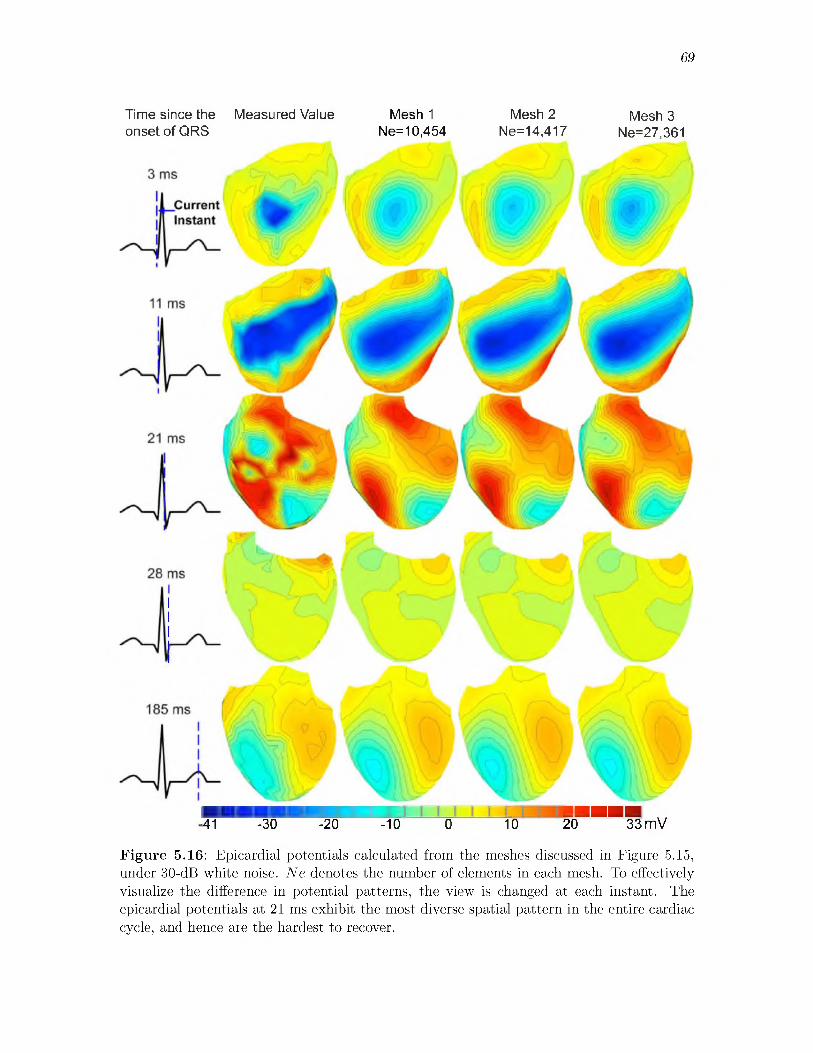
69
Time since the Measured Value Mesh 1 Mesh 2 Mesh 3onset of QRS Ne=10,454 Ne=14,417 Ne=27,361
■■■■■■I JUUUU w■41 -30 -20 -10 0 10 20 33 mV
Figure 5.16: Epicardial potentials calculated from the meshes discussed in Figure 5.15, under 30-dB white noise. Ne denotes the number of elements in each mesh. To effectively visualize the difference in potential patterns, the view is changed at each instant. The epicardial potentials at 21 ms exhibit the most diverse spatial pattern in the entire cardiac cycle, and hence are the hardest to recover.

70
Figure 5.17: Activation isochrones derived from reconstructed epicardial potentials in Figure 5.16. Top row: the anterior view. Bottom row: the posterior view.
Figure 5.18: (A): a cross section of the torso mesh, where the heart is surrounded by 2 layers of prism elements. (B): the hybrid mesh at the heart-volume interface.

71
5.5.5 R efin ing the N orm al D irection
In this test, we explored the impact of the resolution in the normal direction by refining
a region of prism layers around the heart while fixing the rest of the volume mesh. We set the “prism zone” to be within 10 mm from the epicardium, and create three hybrid meshes
having 1, 2 and 4 layers of prisms within the “10-mm prism zone.” The thickness of prisms
are 10 mm, 5 mm, and 2.5 mm accordingly. All three meshes share a coarse tetrahedral
mesh in the volume (8106 tetrahedra), which is fixed so as to isolate the effects of refinement
in the normal direction. To highlight the effect induced by prisms, we compared the hybrid
meshes with a pure tetrahedral mesh in approximate resolution.
Figure 5.19 presents the singular values of the heart-to-volume projector, A VH, and the
transfer matrix, K. Compared with the pure tetrahedral mesh, all three hybrid meshes improve A vh significantly and improve K moderately. Panel B shows that refining the normal direction beyond a certain level may not bring much difference in the resulting
numerical system. Figure 5.20 compares the activation maps derived from the reconstructed
epicardial potentials. Hybrid meshes result in better recovery of activation isochrones.The effect of the normal-direction resolution became more evident when the inverse
problem was solved by the gradient-oriented first-order Tikhonov (FOT). We implemented
the FOT using the variational-formed gradient operator. Figure 5.21 shows the recovered
epicardial potentials at a representative instant when the potentials exhibit the most diverse spatial pattern. Refining the normal direction improves RE and CC slightly, but recovers
Figure 5.19: Refining the resolution normal to the heart by prismatic elements. (A): singular values of A VH. (B): singular values of K.

72
185 190 195 200 205 210 mS
Figure 5.20: Activation times derived from epicardial potentials calculated from the meshes in Figure 5.19. (A): from measured potentials. (B): from the pure tetrahedral mesh. (C): from the hybrid mesh with 1 layer of 10-mm-thick prisms. (D): from the hybrid mesh with 2 layers of 5-mm-thick prisms. (E): from the hybrid mesh with 4 layers of 2.5-mm-thick prisms.
20 -10 0 10 20 30 mV
Figure 5.21: Epicardial potentials computed from hybrid meshes. (A): exact value. (B): pure tetrahedral mesh. (C): hybrid mesh with 1 layer of prisms. (D): hybrid mesh with 2 layers of prisms. (E): hybrid mesh with 4 layers of prisms. rgrad is the ratio of the computed value to the real value of ||VuH||, the L2 norm of the epicardial potential gradient field.
a larger proportion of the potential gradient field on the epicardium, as indicated by rgrad
rising from 76% to 91%. An important goal in inverse calculation is to faithfully reconstruct the sharp gradients in the true inverse solution. On the other hand, the Tikhonov method
tends to over-smooth its inverse solution.Such improvement is achieved in two ways. First, refinement in the normal direction
assumes higher gradients to be represented by discretization, thereby improving the transfer
matrix. Second, the refinement increases the magnitude of the stiffness matrix, which then
enhances the regularizing effect of the variational gradient operator (based on the stiffness
matrix). This test exemplifies how discretization choices may achieve regularization effects

73
and affect inverse solutions.
5.5.6 V olu m e R efinem ent w ith the H yb rid M esh
This section is meant to be a comparative study to the volume-refining test presented
in Section 5.5.3, which uses pure tetrahedral meshes. With tetrahedral meshes, refining
the volume inevitably changes the discretization of the heart-to-volume interface. With the
hybrid mesh, we were able to isolate the impact of volume refinement by fixing the prism
mesh around the heart while refining the rest of the volume. We set two layers of 5-mm-thick
prisms so as to reasonably approximate the gradient field around the heart. Fixing both the prismatic mesh and the torso-surface triangulation, we tetrahedralized the rest of the
torso volume with three resolutions, respectively. Figure 5.22 presents the resulting A VH,
N, and K. It confirms our conjecture that the extension of the singular value spectra of N
and K is attributed to the refinement of the interior volume, but not to the refinement of
the heart-volume interface. Note that the matrix A vh was fixed in this test because the discretization of the heart-volume interface was fixed by the prismatic mesh.
5.5 .7 D iscussionThe primary goal of our discretization study was to explore how the finite element
discretization of the ECG model influences the numerical conditioning of the inverse ECG problem, so as to formulate a numerical problem optimal for inverse calculation. While
many research studies have been devoted to stabilizing the ill-posedness by various regu-
Singular Value Index Singular Value Index
Figure 5.22: Refining the volume while fixing the meshes around the heart by two layers of 5-mm-thick prisms. Mesh 1, 2, and 3 contain 8106, 13636, and 23361 tetrahedral elements. (A): singular values of N and A VH. (B): singular values of K.

74
larization techniques, few studies concentrated efforts on improving the numerical quality
of inverse problems before their inverse solutions are sought. In fact, proper discretization
strategies can be used in combination with regularization methods so as to achieve additional improvement to the inverse solution accuracy.
To assess the impact of discretization, our methodology included testing different finite element discretization strategies and then evaluating their resulting transfer matrix (the
inverse problem) by singular value analysis. We then evaluated the inverse solutions in
terms of quantitative metrics, epicardial potential patterns, and activation isochrone maps.
The inverse solutions are calculated by a fixed regularization method (mostly second-order Tikhonov) in order to isolate the effect of discretization and to minimize the effect of
regularization.
Our experiments based on 3D models obtained consistent results with our previous study
based on 2D models presented in Section 5.4. Our results corroborate the inverse-problem
discretization guidelines proposed in Section 5.3. Figure 5.14 indicates that the epicardial
resolution for which we seek should be limited based on practical needs lest the discretized inverse problem become overly ill-conditioned. Meanwhile, refining the volume conductor
improves the conditioning of the transfer matrix (Figure 5.15), the reconstructed epicardial
potentials (Figure 5.16), and activation isochrones (Figure 5.17).The use of hybrid meshes enables one to refine the high gradient field around the heart
without incurring aspect-ratio problems. Such refinement improves the accuracy of the
heart-to-volume projection (Figure 5.19) and the reconstruction of epicardial potential gradients (Figure 5.21), which in turn improves the recovery of the activation isochrone
map (Figure 5.20). It is worth comparing the refinement in the normal direction to the
heart to previous studies that use the potential gradient or current density (from a physical view) as a constraint in regularizing the inverse ECG problem [37]. The spatial refinement
implicitly assumes that a higher gradient is being sought, so it achieves a similar regularizing effect often referred to as “regularization by discretization” [29, 28].
The CPU time of our ECG simulation consists of (1) the time for building the FE model and the minimization problem and (2) the time for solving the minimization. The first time
is dominant and is linear in the number of elements being used. Hybrid meshes enable us to
improve accuracy without dramatically increasing the mesh size and hence the CPU time. The time for carrying out the Tikhonov regularization given by Equation (5.10) (for each
value of A) is 1-2 seconds in Matlab with four 2.66-GHz Intel Xeon cores, when the transfer
matrix K was of the size 771 x 337 (the number of nodes on the torso surface and the heart
75
surface, respectively).
5.6 Adapted p-Type Finite Element RefinementSo far our study on refinement of the finite element method (FEM) for the inverse
problem has concentrated on the spatial, or h-type refinement. As we have discussed in Chapter 2.2.2, the p-type refinement, using high-order finite elements, usually improves
approximation accuracy more efficiently than the h-refinement. In this section, we explored the use of high-order finite elements to improve the discretization of the inverse ECG
problem.We found that high-order elements need adaptation in order to be suitable for the
inverse problem. As indicated by Figure 2.7, the basic form of high-order finite elements is equivalent to uniform refinement, incorporating higher-spatial-frequency components into
inverse calculation. The property of such uniform refinement has been demonstrated to
be inappropriate for inverse calculation (see Section 5.2). On the other hand, as we have discussed in Section 5.3, the refinement guidelines for our inverse ECG problem suggest refining the torso volume while limiting the discretization resolution on the heart surface.
To fulfill this goal, we proposed an adapted p-refinement scheme as illustrated in Fig
ure 5.23. This scheme uses regular high-order finite elements except at interfaces where a low-order approximation is needed (e.g., the heart boundary). At any such interface, we
adopted only the linear edge modes (and discarded the rest edge modes) among the full modal expansions within the element adjacent to that interface. Note that our selective
extraction of edge modes is made possible by the special property of our modal expansions:
because all the face modes in this modal expansions are zero-valued at element boundaries, the face modes are not affected by the removal of some edge modes.
With our adaptive p-refinement scheme in place, we fulfilled our inverse-problem-oriented
refinement guidelines in the following way: we performed p-refinement in the torso volume
while fixing a linear finite element discretization on the heart and torso surface. The goal
of fixing the discretization on the heart surface was to constrain the ill-conditioning of
the numerical inverse problem. Our decision to represent the torso surface by linear finite
elements was based on two considerations. First, the measured torso-surface potentials are available only at a limited number of mesh nodes, so one does not have verified torso-
potential information beyond the linear vertex modes. Second, the torso-surface potential field is sufficiently smooth for linear elements to attain satisfactory accuracy.
We now demonstrate how our p-refinement scheme improves the numerical accuracy of
our inverse problem. To simplify our presentation, we assume that quadratic finite elements

76
Figure 5.23: Illustration of triangular finite elements using third-order modal expansions in the torso volume while keeping first-order (linear) expansions on the torso and heart boundaries. The modal basis expansions are illustrated in Figure 2.8. The red nodes denote the vertex modes (the element-wise linear component). The blue nodes denote the edge modes, and the green nodes denote the face modes.
are being used in the torso volume whereas linear elements are used on the heart and torso boundaries. Recall that the finite element solution of our partial differential equation is
given by Equation 4.2, which we rewrite here:
A vva tv
a vtA tt
uvut
- A vh- A th
uh (5.12)
where the subscripts represent the location group to which each basis function belongs: H
stands for the heart boundary, T for the torso boundary, and V for the torso volume.Given the use of modal quadratic elements, we rearranged all the global basis functions
according to their polynomial order: the first group consists of element-wise linear basis
functions, the second group consists of element-wise quadratic basis functions, and so on (if
there are finite elements above the second order). We rearranged the coefficient associated with each basis function in the same order. To manifest such grouping, Equation (5.12) can
be expressed in a more detailed form as follows:
/ A i’ia vv A 1,2
vvA 2,1 A 2’2 a vv a vvA 1’1 \ a tv A 1,2
TV
1,1vt2,1vt
1
A 1,1
u
u
A 1,1a vh
TT / \ uT /
A 2,1vh
1,1
uH (5.13)
\ a th j
Here the subscripts have the same meaning, and the superscripts represent the order of2,1each basis function. For example, A y H denotes the stiffness matrix formed by coupling

77
the element-wise second-order basis in the volume (V) and the element-wise linear basis on
the heart boundary (H ). The same notation applies to the vectors of unknown coefficients:
uT denotes the coefficients for the element-wise linear components on the torso boundary, whereas uV denotes the coefficients for the element-wise quadratic components in the torso
volume.The numerical formulation of the inverse problem, or specifically the transfer matrix K,
is given by Equation 4.10, and we rewrite it here. Assuming only the linear finite elements are used, we place superscript 1,1 on all terms:
When quadratic elements are used, the transfer matrix K is derived in the same way but containing augmented terms:
Comparing Equation (5.14) and (5.17), one can see how the p-refinement improves the discretization of the inverse problem. The quadratic finite element system not only
encompasses the linear finite element system, but also incorporates extra second-order
information. The second-order information takes effect via the stiffness matrices A v v , A v t ,
and A vh , then being incorporated into the matrices M and N. Note that both M and N
need the calculation of the inverse of A vv , which is also the most computationally intensive
step in calculating K. In fact, A vv exactly arises from solving the homogeneous elliptic problem given by Equation (5.8). This fact explains why the p-refinement leads to a more
accurate A v v , which in turn improves the numerical formulation of the inverse problem. During our p-refinement, although the matrices K, M, and N do not change their sizes,
they implicitly incorporate high-order (high spatial frequency) information of the continuum
field they approximate.
uT = KuH, K = M - 1N; (5.14)
(5.15)
(5.16)
uT = KuH, K = M / - 1N ; (5.17)1,1 1,2 1 1,1
(5.18)
(5.19)
5.6.1 C om p arison o f the h -T yp e and p -T y p e R efinem entsOur p-refinement strategy proposed in this section and our h-refinement strategy pre
sented in the previous section can be unified under the same discretization approach we
78
discussed in Section 5.3, which states that the discretization for our inverse ECG problem
revolves around three objectives: (1) approximating the heart boundary, (2) approximating
the heart-to-torso interface, and (3) approximating the torso volume. Both our h-type and p-type refinements increase the accuracy of the second and third objectives.
The h-refinement increases the approximation accuracy by reducing the spatial grid size,
whereas the p-refinement does so by using high-order basis polynomials. To attain the goal of refining the heart-to-torso interface while preserving the resolution on the heart boundary,
our h-refinement uses hybrid-shaped finite elements, involving the use of quadrilateral or prismatic elements in order to decouple the discretization in the normal direction and at the
heart surface. In comparison, our p-refinement extracts the vertex modes and removes the
high-order edge modes that live on the heart boundary. Essentially, the adaptation fulfilled
by hybrid-shaped elements is “spatial,” whereas the adaptation fulfilled in the high-order finite elements is performed in the hierarchical polynomial space defined over each element.
Because of the nature of hierarchical modal expansion, the adaptation in the polynomial
space constitutes a seamless solution for selective refinement, enabling the approximate
solution to maintain a good smoothness and circumventing the aspect-ratio problem that obstructs spatial refinement methods. These nice properties make our adaptive p-refinement
often advantageous to spatial refinement.
5.6.2 Im plem en tationWhen implementing the high-order FEM, one needs to keep track of each basis function's
global number and its local number within each element that contains that basis function.
Our adapted p-refinement scheme omits some basis functions in certain edges or faces
depending on our needs. The task of tracking which basis functions are omitted, both in global and local numbering systems, becomes very complicated in three-dimensional
meshes, because there are many topological possibilities for the local numbering scheme in
an element.However, because the basis functions we used are modal and can be decomposed into the
vertex/edge/face modes, keeping track of the numbering of basis functions becomes much simpler than it appears to be. The first step is to carry out a regular uniform p-refinement,
resulting in a matrix equation in the form of Equation (5.12), with all the basis functions
and coefficients being labeled by their polynomial order and type of modes (vertex, edge,
or face). The second step is to remove all the rows and columns corresponding to the basis functions we want to omit. This step is justified because all the modal basis functions are
independent of each other, and each basis function impacts only its corresponding row and
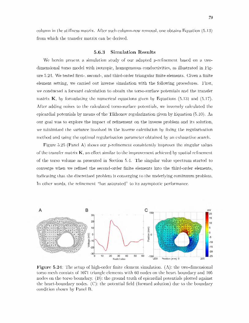
79
column in the stiffness matrix. After such column-row removal, one obtains Equation (5.13) from which the transfer matrix can be derived.
5.6.3 S im ulation R esu lts
We herein present a simulation study of our adapted p-refinement based on a two
dimensional torso model with isotropic, homogeneous conductivities, as illustrated in Fig
ure 5.24. We tested first-, second-, and third-order triangular finite elements. Given a finite element setting, we carried out inverse simulation with the following procedures. First,
we conducted a forward calculation to obtain the torso-surface potentials and the transfer
matrix K, by formulating the numerical equations given by Equations (5.13) and (5.17).
After adding noises to the calculated torso-surface potentials, we inversely calculated the
epicardial potentials by means of the Tikhonov regularization given by Equation (5.10). As our goal was to explore the impact of refinement on the inverse problem and its solution,
we minimized the variance involved in the inverse calculation by fixing the regularization
method and using the optimal regularization parameter obtained by an exhaustive search.Figure 5.25 (Panel A) shows our p-refinement consistently improves the singular values
of the transfer matrix K, an effect similar to the improvement achieved by spatial refinement
of the torso volume as presented in Section 5.4. The singular value spectrum started to converge when we refined the second-order finite elements into the third-order elements,
indicating that the discretized problem is converging to the underlying continuum problem.
In other words, the refinement “has saturated” to its asymptotic performance.
Node Index -200 Position (mm) 0 200
Figure 5.24: The setup of high-order finite element simulation. (A): the two-dimensional torso mesh consists of 1071 triangle elements with 60 nodes on the heart boundary and 105 nodes on the torso boundary. (B): the ground truth of epicardial potentials plotted against the heart-boundary nodes. (C): the potential field (forward solution) due to the boundary condition shown by Panel B.
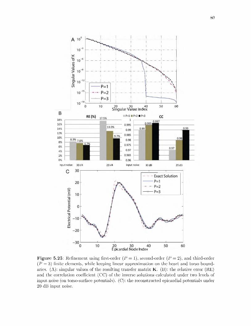
80
10 20 30 40
B18%16%14%12%
10%
6%4%2%0%
Singular Value Index50 60
Input noise: 30 dB 20 dB Input noise: 30 dB 20 dB
E picardial Node Index
Figure 5.25: Refinement using first-order (P = 1), second-order (P = 2), and third-order (P = 3) finite elements, while keeping linear approximation on the heart and torso boundaries. (A): singular values of the resulting transfer matrix K. (B): the relative error (RE) and the correlation coefficient (CC) of the inverse solutions calculated under two levels of input noise (on torso-surface potentials). (C): the reconstructed epicardial potentials under 20 dB input noise.

81
Figure 5.25 (Panel B) assesses the inverse solution by its relative error (RE, defined
in Equation (5.9)) and its correlation coefficient (CC, defined by Equation 5.11) with the
ground truth. The inverse solution was calculated with zero-mean Gaussian noise of 30 dB and 20 dB being added to the torso measurements. The result shows that our adapted high-order refinements effectively reduce the error and improve the correlation coefficient.
Figure 5.25 (Panel C) displays an example of the recovered epicardial potentials under 20
dB noise, again showing that the third-order finite element method yields the best solution.
5.7 Regularization in Variational FormsMost traditional regularization techniques solve a given inverse problem at an algebraic
level, assuming the inverse problem is being given in the form of an algebraic system that is a
numerical approximation of the underlying continuum problem. This approach is confronted
with a common problem that the regularization may yield inconsistent results when the
inverse problem is discretized into different scales, because an algebraic system by itself does not reveal how it is formed from the continuum problem. In view of this problem,
we formulated in this section a new family of regularization terms (also called regularizers)
that ensure consistency for multiscale simulation of inverse problems.Our regularizers are formed based on the variational principle underlying the finite
element method (FEM), and fit into the classic Tikhonov regularization framework, serving as an alternative to the traditional algebraic-form Tikhonov regularizers but featuring
several advantages. First, the variational regularizers keep the connection between the discretized model and its underlying continuum model, and automatically conform to certain variational properties inherently assumed by the discrete model resulting from the FEM.
Second, the variational regularizers preserve their norms, and thereby maintain consistent
regularization when the inverse ECG problem is simulated under multiple scales. Third, the variational formulation facilitates construction of the discrete gradient operator, which
is normally difficult to obtain over irregular meshes. Fourth, it allows efficient imposition
of multiple constraints simultaneously.
5.7.1 Form ulation o f R egu larizers
We present the formulation of our regularizers within the Tikhonov framework of Equa
tion 5.10. We borrow the name “variational” from the context of FEM, upon which the for
mulation is based. The main idea is to consider the epicardial potentials not as a vector, but as a continuous function represented by finite element expansion: UH(x) = ^ k ukH0 k(x), k £
H . The potential field is evaluated by the continuous L2 norm, which is defined as:

82
||Uh ||l2 = (Uh ,Uh ) 1/2 = ( J uh Uh . (5.20)
Substituting the finite element expansion into (5.20) yields
II(Uh)\?l2 = uH , ^ uH ) = uHM uh , = (0 i , 0 i ); (5.21)i j
where M is the mass matrix over the heart. Similarly, one may evaluate the L2 norm of
the potential gradient field by
IIVUhIIL2 = ( ^ uHV0 i, ^ uHV^j) = uHSuh, Si,j = (V 0 i, V ^ j); (5.22)i j
where S is the stiffness matrix over the heart. More discussion of M and S is presented in
Table 5.4. The Euclidean norm || ■ ||2 with an operator L has the property that ||Luh||2 =
uHLt Luh . Hence, if L is to describe the magnitude of the field Uh , it should satisfy Lt L = M. Such L can be computed as the Cholesky factor of M and can be used in
Equation (5.10) for the zero-order Tikhonov regularization, as opposed to the traditional choice of an identity matrix.
If L is to describe the gradient field VUH, it should satisfy LTL = S, or equivalently be the Cholesky factor of S. We name such L the “variational-form” gradient operator because
it is equivalent to the real gradient operator in the variational sense. The variational gradient
operator L can be used in Equation (5.10) to fulfill the first-order Tikhonov regularization.
Table 5.4 compares variational-formed operators with traditional operators up to the
second order (the surface Laplacian). One may extend this formulation to operators regarding even higher-order Sobolev norms, provided that the finite elements maintain stronger
differentiability— for example, the variational Laplacian operator requires finite elements to be at least C 1 continuous, and the variational version of higher-order operators may need
C P continuous elements. In this chapter, we only consider C0 elements and accordingly,
constraints up to first-order derivatives.
The Cholesky decomposition always exists because the mass matrix, the stiffness matrix, and matrices formed by higher-order derivatives are symmetric and at least positive-semi-
definite. More discussion of the Cholesky decomposition will be presented in Section 5.7.6.
5.7.2 N orm P reservationOne advantage of the variational-form operators over conventional discrete operators is
that the former preserves the norms under different resolutions - the continuous L2 norm is

83
Table 5.4: The choice of L for Tikhonov Regularization.
Regularization Type Conventional Regularizer Variational RegularizerZero-order Tikhonov Identity MatrixFirst-order Tikhonov Hard to Define
Second-order Tikhonov Discrete Laplacian Operator
Lt L = M Lt L = S
Lt L = Qt
L is associated with mesh nodes on the heart surface. The matrices M, S, and Q are given by Mi,j = ( & , $ j ), Si,j = (V 0 i, V ^ j), and Qi,j = (V2^ , V 2^-), i , j £ H .
f Formulation of Q requires at least C 1 continuous elements.
independent of the discretization resolution, and the weights made by FEM basis functions
take mesh spacing into account. Consequently, the variational operators achieve consistent
regularization when the inverse problem is computed under multiple scales. In contrast, conventional regularizers are evaluated by the Euclidean norm, which heavily relies on the
discretization resolution and cannot effectively relate the discrete model with its underlying
continuous field.Taking the zero-order Tikhonov for example with the variational regularizer, changing
mesh spacing affects basis functions and then the mass matrix, so the L2 norm of epicardial
potentials is preserved. With the conventional identity matrix, however, the regularizer’s Euclidean norm is sensitive to the mesh resolution.
Tikhonov regularization with multiple spatial/temporal constraints [3, 15] is often de
sirable. Each constraint imposes its own bias on the inverse solution, so combining several constraints may moderate the bias and provide a more comprehensive account of the
solution. Inverse solutions are sensitive to the values of regularization parameters. By
distributing regularization to multiple constraints, one may improve the robustness of the
solution to any individual parameter.
The Tikhonov regularization with multiple constraints is expressed as follows:
merical stability in practice, the minimization is achieved by solving a linear least-squares problem of the form:
5.7.3 Im p osition o f M u ltip le V ariational R egu larizers
uh = argmin ||Kuh — u t ||2 + E 2 II LiuH1122. (5.23)
Its solution is conceptually expressed as uH = (K TK + ^ i A2(LTLi)) 1K TuT. For nu-
(5.24)
84
where L denotes a concatenation of all Lis. Equation (5.24) can be solved by standard routines such as the QR factorization, or most efficiently by the bidiagonalization algorithm [27].
With multiple constraints, AL is made by concatenating each AiLi. Note that although
(5.24) is in the Euclidean norm, if Li is the variational regularizer, ||Luh||2 actually gives
the value of the continuous L2 norm.To further promote efficiency, one may construct a compact constraint, denoted as L*,
which is equivalent to the superposition of all constraints:
L*t L* = ^A2||l TLi||2, Ai = 0. (5.25)i= 1
Equation (5.24) then substitutes L* for all Lis. Moreover, since only the term LTLi is
needed, one may directly use the mass matrix or the stiffness matrix, without factorizing
each Li. The compact operator greatly saves memory when the problem size is large and
there are many constraints. The compact operator also improves efficiency when all Ais
need to be optimized over a large number of admissible values.
5.7.4 G radien t O p era tor B ased on M esh N od esA noteworthy feature of our variational formulation is that it enables a simple construc
tion of a closed-form discrete gradient operator defined over mesh nodes, an operator that is traditionally difficult to derive over irregular meshes. The closed-form gradient operator,
denoted by LG, is defined as follows: given a potential field uH located on the nodes of
a mesh, LG is a matrix such that LGuH gives the magnitude of V u H (a vector at each
node) located on the same set of nodes. The gradient operator plays an important role
in PDE-constrained optimization as a basis for Newton’s method. For our inverse ECG
problem, the gradient operator over a heart surface enables gradient-based regularization
methods, which have been reported to yield superior recovery of the spatio-temporal char
acteristics of epicardial data, such as the first-order Tikhonov [109, 71] or the total-variation regularization [37].
Although a gradient field is not difficult to compute (by Taylor approximation or the
Gauss-Green theorem), it is difficult to derive an accurate discrete gradient operator in a closed, matrix form, especially on irregular, unstructured meshes. The matrix form requires
representing the gradient at one node by the data at its neighboring nodes, an ill-posed
problem when mesh nodes are irregularly distributed. (Here irregularity means that if we set a node as the center, its adjacent nodes are not distributed in uniform angles with respect
to the center node.) One study [37] obtained the gradient operator over the heart surface

85
via the boundary element method (BEM) for the Laplace’s equation. This derivation can
be found in Equation (13) in [9]. However, such construction of the gradient operator does
not translate itself into finite element methods, because the FEM and BEM treat boundary conditions differently. The BEM includes both the Neumann boundary condition and the
Dirichlet boundary condition on the heart surface, thus enabling a gradient operator relating
the two. In contrast, the FEM only includes the Neumann boundary condition, treating
the Dirichlet boundary condition as an external “forcing term” (see Section 2.2.1), so the
gradient operator cannot be directly formed from the FEM.In contrast, it is straightforward to construct a variational-form gradient operator by
following Equation (5.22). Note that the variational gradient operator is equivalent to the “true” node-based gradient operator (even if it exists as a conceptual term) in the sense of
being evaluated by the L2-norm but not in the pointwise sense.
5.7.5 N um erica l S im ulation
5.7.5 .1 S im ulation SetupThe setting of this simulation experiment is the same as the experiment described in
Section 5.5.1, regarding the geometric model and the heart voltage data being used. The
heart and torso geometries are depicted in Figure 5.18. The benchmark mesh used in this study consisted of 27,361 tetrahedral elements in the torso volume, with the heart surface
consisting of 337 nodes and 670 triangles, and the torso surface consisting of 771 nodes and
1538 triangles.
5 .7 .5 .2 V ariational G radien t R egu larizer
This test demonstrated the efficacy of the variational gradient operator given by Table 5.4 when used in the first-order Tikhonov regularization (FOT). We compared the FOT
with conventional zero-order Tikhonov (ZOT) and second-order Tikhonov (SOT). The ZOT
used an identity matrix as the regularizer. The SOT used a discrete Laplacian operator obtained by solving a least-square problem arising from second-order Taylor expansion
at each mesh node, as proposed by [52]. Figure 5.26 compares the epicardial potentials
reconstructed by the three methods. Overall, the FOT and SOT performed closely, both outperforming the ZOT. The FOT sometimes outperforms the SOT in capturing local
spatial patterns or iso-potential contours: e.g., the contours at 10 ms, the saddle point
at the heart center at 21 ms, and the iso-potential contours at 27 ms. These observations
agreed with our anticipation, for the Laplacian regularizer tends to smooth contours whereas
the gradient-based regularizer preserves contours better.

86
Time since the Measured Data ZOT FOT SOTQRS onset
Figure 5.26: Epicardial potentials calculated under 30-dB SNR input Gaussian noise. ZOT, FOT, and SOT denote the zero-, first-, and second-order Tikhonov regularization. To better show spatial patterns, the view is slightly rotated.

87
5.7 .5 .3 N o rm P reservation in M u ltisca le S im ulation
As we have discussed, the variational-form operators preserve their norms under multi
scale discretization, because they consider the continuous L2 norm which is irrespective of resolution. In contrast, conventional discrete operators, evaluated by the Euclidean norm,
depend on the resolution of discretization. This test aimed to illustrate the difference
between both types of operators.We compared the traditional regularizer and the variational one under the zero-order
Tikhonov regularization (ZOT). The traditional regularizer was the identity matrix, whereas the variational-formed regularizer was derived from the mass matrix given by Table 5.4.
Each regularizer was tested with two discrete models: the benchmark mesh (denoted by
Mesh 1) and its uniformly-refined version (denoted by Mesh 2). On the heart surface, Mesh 2 has four times as many nodes as Mesh 1; in other words, the discrete problem yielded by Mesh 2 is four times the size of that from Mesh 1.
When carrying out the Tikhonov regularization, we determined the regularizing param
eter A by the corner of the L-shaped curve (hence called L-curve), a parametric plotting of
||LuH| versus the residual error ||KuH — uT||. The L-curve shows the tradeoff between
minimizing the residual error and satisfying the constraint. Figure 5.27 compares the L-curves resulting from the multiscale test of each regularizer. Panel A shows the L-curves
from the identity matrix, and Panel B shows the L-curves from the mass matrix. In PanelA, refinement pushes the L-curve to the upper right, indicating that refinement increases
both the residual error and the constraint (here the solution norm). In contrast, in Panel
B, the L-curve is not significantly affected by refinement. Note that Panel A and Panel B
have different axis scales.
Figure 5.27 marks the value of A associated with the corner of each L-curve, which typically estimates a reasonable amount of regularization one should apply. In Panel B,
both the residual error and the solution norm at the corner are preserved during refinement.
In Panel A, the residual error and the solution norm at the corner are nearly doubled. Recall that the size of the inverse solution vector increases by a factor of four from Mesh 1 to Mesh
2, but ||uH|, the Euclidean norm of the solution vector, is only doubled. This indicates
that the traditional discrete regularizer tends to over-smooth the inverse solution when
discretization is refined, causing inconsistent regularization under multiscale simulations.

88
Figure 5.27: L-curves of the norm of the solution versus the residual error when the zero-order Tikhonov is performed. The inverse problem is discretized in two scales. Mesh1 has 27,361 tetrahedral elements with 670 triangular elements on the heart surface. Mesh2 has 60,617 volume elements with 2,680 triangles on the heart surface. Panel A: the regularizer is the identity matrix, with the residual error and the regularizer evaluated by the Euclidean norm. Panel B: the variational regularizer derived from the mass matrix given by Table 5.4, evaluated by the continuous L2 norm. The A value indicates the regularization parameter corresponding to the corner of L-curves.

89
Such inconsistency is also manifested in Figure 5.28, where we compare the inverse
solutions at a time instant when the epicardial potential pattern is the most diverse. When Mesh 1 was refined to Mesh 2, the identity-matrix regularizer yielded inconsistent potential patterns, with the relative error of the inverse solution increasing from 0.50 to 0.53. In
contrast, the variational-formed regularizer maintained the pattern of the inverse solution
over refinement, reducing the error from 0.48 to 0.42.
5.7.6 D iscussion
The central idea of the variational-form-based regularization is to measure the po
tential field by the L2 norm in place of the Euclidean norm. Because the L2 norm is
inherently assumed by common finite element methods (e.g., Galerkin formulation), the
variational-formed regularization automatically conforms to certain variational principles
Figure 5.28: Epicardial potentials reconstructed under 30-dB SNR input noise by the zero-order Tikhonov using the traditional and the variational regularizers, corresponding to the L-curves in Figure 5.27. For each inverse solution, the relative error (RE) and correlation coefficient (CC) are given.

90
underlying the discrete inverse problem formulated by finite element methods. Defined over a continuous domain, the L2 norm is independent of discretization resolution, thereby
ensuring that the discretized problem is handled in conformity to its underlying continuous
problem. The Euclidean norm, in contrast, does not reflect the features of the continuous problem.
The preservation of norms is important when applied to multiscale simulation of inverse
problems, because it ensures that regularization is performed consistently among numerical
problems of different scales. Here the consistency means that the balance between the
residual error and the regularizing term is maintained. The requirement of consistency is
based on the understanding that all discrete problems should reflect the nature of their
common continuous origin. The consistency cannot hold when the Euclidean norm is used. When conventional discrete operators are used in Tikhonov regularization, the residual error
and the regularizer may not increase in the same rate under refinement. If the residual
error increases faster than the regularizer, more weight will be put on the residual error
and the inverse problem tends to be under-regularized. Conversely, the inverse problem will be over-regularized. In our example of testing the zero-order Tikhonov method under
multiscale discretization, Figure 5.27 shows that the preservation of the L2 norm leads to
consistent regularization, which consequently leads to consistent reconstruction of epicardial
potentials, as shown by Figure 5.28. The traditional Euclidean-norm-based regularization does not exhibit the consistency.
The introduction of resolution-consistent regularization may pave the way for adaptive
finite element methods to be used for solving inverse problems. Despite its many successes in reducing complexity and enhancing efficiency for solving PDE-based forward problems, the
adaptive FEM has not yet been widely applied to inverse problems. By taking advantage
of their natural consistency within the FEM Galerkin framework, resolution-consistent regularization may solve the issues that arise with nonuniform volumetric resolution.
It is straightforward to implement the variational-formed regularization in the L2 norm by slightly modifying the implementation of traditional Tikhonov methods. The Euclidean
norm of the epicardial potentials uH is given by ||uH||2 = (uHuH)1/2, whereas the L2 norm
of the continuous distribution UH is given by ||UH||L2 = (uHMuH) where the mass matrix M is given in Table 5.4. Evaluating the L2 norm is achieved by adding a weighing matrix
that is based on finite element basis functions. The norm of the residual error defined on
the torso surface, or the norm of any gradient field, can be obtained in a similar way by
modifying the weighing matrix accordingly. The weighing matrix can be precomputed using

91
the mesh information alone.
The stiffness matrix and matrices formed by higher-order derivatives are positive-semi-
definite because the derivative of any constant field is always zero. The Cholesky decomposition for these matrices is not unique, but we do not believe this fact will effect the outcome of Tikhonov regularization because the Tikhonov method considers the L2 norm
of the regularizers. We selected a Cholesky factorization in a systematic way. Assume we
decompose the stiffness matrix S. We take the sequence Sk = S + k I, where I is the
identity matrix. Sk ^ S when k ^ rc>. Each (S fc } is positive-definite and has a unique Cholesky factor Lk. We take L = limk ^ Lk as the Cholesky factor of S. The convergence
of {L k} holds because the operators are bounded and their underlying vector space is finite dimensional.

CHAPTER 6
BIDOMAIN-BASED INVERSE ECG PROBLEM
This study aimed to reconstruct the transmembrane potential (TMP) throughout the myocardium based on the bidomain model, and to apply the reconstruction to localizing
myocardial ischemia. Our main contribution lied in solving the inverse problem by a
PDE-constrained optimization framework, with which we derived solutions for the L2-norm
Tikhonov regularization and the L1-norm total variation minimization. The subsequent
numerical optimization was fulfilled by a primal-dual interior-point method tailored to our
problem’s specific structure. Simulation was conducted using a realistic, fiber-included anatomical model with experimental ischemia data.
6.1 IntroductionAs we have mentioned in Section 2.1.3, myocardial ischemia can be characterized by the
bidomain heart model via myocardial transmembrane potentials. Traditional clinical ECG
diagnosis, relying on expert interpretation of body-surface recordings, has limited ability to localize ischemic regions and moreover, even the epicardial potentials are insufficient for such
localization [74]. Therefore, the ability to inversely reconstruct a whole-heart TMP map from body-surface recordings would greatly promote robust determination of the location and extent of ischemia in patients.
As has been reviewed in Section 3.1.4, the inverse problem of reconstructing myocardial
TMPs has seen limited progress because the task is even more difficult than other types of inverse ECG problems. While the goal of reproducing the TMP at an arbitrary time
instant remains unresolved, it appears more tractable to solve the simplified problem of re
constructing ischemia-induced TMP amplitude variations, and thereby achieves a satisfying
localization of the disease. This assumption, discussed in Section 2.1.3, forms the rationale of this study.
93
Our major contribution lies in the formulation of a new inverse-calculation methodology
called PDE-constrained optimization. Inverse ECG problems are conventionally solved within the following scheme: based on the underlying physical model, one first forms an explicit “transfer” model that maps the unknown source parameters to the measurements;
with that transfer model (typically in a matrix form), one then obtains the solution by mini
mizing the misfit between the predicted and measured data. The minimization process may
incorporate some regularization constraints if there is a need to mitigate ill-conditioning.
This approach, because it is founded on the “transfer” model, allows constraints only on
the source parameters, and thus becomes inadequate for complex source models such as the bidomain model. In contrast, our approach treats the inverse problem as a constrained
optimization problem that incorporates the whole governing PDEs as a constraint. This
approach, known as PDE-constrained optimization, offers ample flexibility not only for
adjusting the underlying physical model but also for applying various physically-based
constraints simultaneously.PDE-constrained optimization has been a frontier in scientific computing research over
the last decade, and abundant theoretical accomplishments [48] have laid the foundation
for its practical application. Its initial introduction to ECG problems [85] was limited
to quadratic objective functions with equality constraints. In this study, we extend that
inaugural work by allowing general objective functions and constraints in both equality and inequality forms.
Numerical solutions of PDE-constrained optimization typically involve forming the opti
mality conditions and then solving them by variants of Newton’s method. In several aspects, this task is much more challenging than solving an ordinary optimization problem or a PDE
alone. First, most existing PDE solvers cannot be directly used when a PDE becomes a
constraint in optimization. Second, the large size of the discretized PDE constraints poses a challenge for contemporary optimization algorithms. This challenge is compounded by
the iterative nature of most optimization procedures, meaning that each iteration requires a full solution of all PDEs.
To tackle these difficulties, one needs not only to efficiently integrate generic optimization
algorithms, advanced PDE solvers such as adaptive finite element methods, and large-scale
scalable linear solvers such as the Newton-Krylov method [11], but also to create a frame
that exploits the mathematical structure specific to the domain of science being considered,
in our case, electrophysiology. Such integration has yet to be fulfilled. Rather, the practice
of typical engineering studies is to discretize the inverse problem over a predefined mesh
94
and then apply standard numerical optimization methods. However, such a practice is not necessarily mathematically rigorous and hence may result in inconsistency when different
meshes are used.In this chapter, we investigate the formulation, discretization, and numerical solution of
our PDE-constrained optimization framework in terms of the finite element method (FEM). We consider two minimization schemes: the Tikhonov regularization and the total variation
minimization. Our contribution features the following new ingredients:
• Formulation of the optimality conditions in the continuous function spaces before discretization, making our optimization algorithms independent of discretization choices.
Such independence brings three benefits: (1) consistent results over multiscale simula
tions, (2) individualized discretization of each variable, and (3) adaptive finite element refinement as the optimization iteration proceeds.
• Detailed comparison between the above approach and the discretize-then-optimize
• Robust finite element formulation of the optimality conditions, for both the Tikhonov
and the total variation regularization.
• Inclusion of inequality constraints, handled by a tailored primal-dual interior-point method presented in a block-matrix form.
This chapter will address all these issues except the adaptive refinement over iterations,
which we defer to future work.
6.2 Inverse Solution by PDE-Constrained OptimizationThe mathematical model of the bidomain-based inverse problem has been presented in
Section 4.2. All the variable notations in that section are inherited in this chapter. We
formulate this inverse problem as a PDE-constrained optimization problem expressed in an
abstract form as follows:
In the optimization community, v and u are often known as the control variable and state
variable, respectively. The first term of the functional J is the misfit between predicted and
observed data, measured by a certain Lp norm at the body surface T . The operator Q :
approach.
minimize J (u,v) = ||Qu - d||Lp(T) + ^||W(v - vo)|Up(H),
subject to e(u, v) = 0, c1(u) e Ku, c2(v) e Kv.
(6.1a)
(6.1b)

95
H1(Q) ^ Lp(T ) is the volume-to-surface projector. The second term of J is a regularization term for stabilizing the minimization. The operator W : H1(H ) ^ Lp(H ) defines certain
regularity conditions to be imposed on v. Common choices for W(v) are v, Vv, or Av. The parameter > 0 controls the amount of regularization. e(u, v) = 0 is an abstract notation
for the physical model. In our problem, it refers to the PDE given by Equation (4.19) with
proper boundary conditions. The last two constraints represent abstract inequality bounds
for u and v, with Ku and Kv denoting proper cones.In the following three sections, we will elaborate on how to populate the abstract concept
presented above in practical simulations in the context of finite element methods. Our
goal is to translate the mathematical formulation into a numerical system for efficient
numerical optimization. In particular, we will address the following four topics in the
subsequent subsections: (1) Tikhonov regularization, (2) finite element formulation of the PDE constraint, (3) total variation regularization and its finite element formulation, and
(4) inequality constraints and a primal-dual method for numerical optimization.
6.3 Tikhonov RegularizationAs one of the most popular approaches to regularizing ill-conditioned inverse problems,
the Tikhonov regularization uses the L2 norm for the objective functional given by Equation
(6.1a), which becomes:
1 BJ (u,v) = 2 llQu — dllL2(T) + 2 |W (v — vo)llL2(H). (6.2)
Because of its quadratic nature, the Tikhonov regularization can be readily integrated with the variational formulation of the optimality conditions to be described in the next section.
When the regularizer is of the Sobolev-norm type such as W(v) = v, Vv, or Av, we can
compute it via a finite element formulation as given in [119]:
llv llL2(H) = vTM v (M )i,j = (^ )H; llV v ll|2(H) = vTS^ (S)i,j = (V^ V ^ j)H (6.3)
where M and S are the mass and stiffness matrices, respectively, based on the finite element
discretization of v. Their Cholesky factor conceptually serves as the equivalent of W, but the Cholesky factorization is not necessary when carrying out the optimization.
Our finite element formulation for W as provided in Equation (6.3) is superior to the common expedient practice of discretizing W directly over a given mesh. Our formulation is
independent of mesh size and therefore not only ensures consistency under multiscale inverse simulation but also allows adaptive refinement during optimization iterations. Moreover,
mesh-grid-based discrete derivative operators are not strictly compatible with the Galerkin

96
finite element discretization because the field has less regularity at nodes than within
elements. This pitfall is overcome in our finite element formulation.
6.4 Treatment of the PDE ConstraintThere are two approaches to numerically tackling the problem given in Equation (2.22):
discretize-then-optimize or optimize-then-discretize. The former approach first discretizes
all the quantities (both the objective and the constraints) into vectors or matrices, and treats the discretized problem as a pure algebraic optimization problem. Alternatively, the
latter approach first derives the optimality conditions in continuous function spaces before discretizing those conditions into numerical systems. Although the former approach is more
popular among the engineering community, the optimize-then-discretize approach typically more faithfully preserves the structure inherent in the underlying infinite-dimensional op
timization problem. This approach is less subject to mesh size, enables individualized
discretization strategies for each quantity, and facilitates adaptive refinement techniques.
We therefore adopted the optimize-then-discretize approach whenever possible. The rest of
this section presents the continuous optimality conditions and their discretization by the
FEM. We will also compare the two approaches and discuss the conditions under which
they are equivalent.For illustration purposes, we minimize the Tikhonov functional given by Equation (6.2),
and assume that the minimization problem is subject only to the PDE constraint given
by Equation (4.19). The Lagrangian functional for this constrained optimization problem,
denoted by L : H1(Q) x H 1(H ) x H-1 (Q) ^ R, is defined as
L (u ,v ,p ) = 2 (Qu - d, Qu - 6) t + § (W(v - vo), W (v - vq) )h + ( p , - V ■ aV u - f )q
(6.4)
where p £ H-1 (Q) is the Lagrange multiplier function. The optimality condition states that the optimal solution is situated at the stationary point of the Lagrangian functional.
By taking the Gateaux derivatives of L at the optimal solution (u, v,p) in the perturbation
direction (u, v,p), we obtain a set of equations as follows:
Lv(u, v ,p )(v) = P (W*W(v - vo),v)h - (aiVp, W ) h = 0, Vv £ H1(H ); (6.5a)
Lu(u, v,p)(u) = (Qu - d, Qu ) t + (aVp, V u )q = 0, Vu £ H1(Q); (6.5b)
Lp(u,v,p)(p) = (aVu, Vp)n - (f,p)n = 0, Vp £ H0(Q). (6.5c)
Equation (6.5) is the variational form of the KKT condition, and Equations (6.5a) - (6.5c)
are called the variational form of the control equation, the adjoint equation, and the state

97
equation, respectively. This set of differential equations is linear with respect to u, v, and
p because the objective is quadratic and the constraint takes the linear equality form. In
general, they are nonlinear PDEs. We now discuss how to discretize them by the FEM.The key to applying the Galerkin finite element discretization to Equation (6.5) is to
take the perturbation in each finite element basis function. We discretize u and v according
to Definition 4.2, and assume that p is discretized by the same trial space as for u:
p ~ Ph = Y1 i=“i Pi,&. Let p = (pi,p2, . .. ,Pnu)T. The perturbation p and u are chosen from the finite-dimensional space {0 i}, and V is chosen from } as given in Definition 4.2. Equation (6.5) then yields a 3 x 3 block-matrix system for numerical computation, given as
follows:
where (■, ■) denotes the inner product defined in Equation (4.9). This forms a symmetric indefinite system where each block is given below:
The remaining task is to numerically solve the large linear system given by Equation (6.6),
which is known to be positive indefinite. Existing methods include the BiStabCG [85], the
adjoint method [48], and computing the Schur complement [14, 113]. In this dissertation, we adopted the Schur complement approach. On the other hand, the adjoint method is widely
used, especially for large-scale linear systems. The adjoint method affects discretization
considerations to be discussed in Section 6.4.1, so we describe it here: the method first
acquires the derivative of the objective J with respect to v (by solving the state and adjoint
equations sequentially), then applies one step of gradient descent of J, and repeats the
above two steps until J is minimized.
6.4.1 O p tim ize -th en -D iscretize versus D iscre tize -th en -O p tim izeIn Section 6.4, we derive the variational optimality condition before applying the finite
element discretization. Here we compare this approach with its alternative discretize-then-
optimize approach. As will be shown, the connection and distinction between the two
approaches are effectively manifested by one fact: the two approaches result in identical numerical optimality conditions only when the state variable u and the adjoint variable p
are discretized by the same trial space. Based on this understanding, we discuss several
theoretical and practical concerns of the two approaches.
c
^M h vo d 0
(6.6)

98
The discretize-then-optimize approach directly applies the finite element discretization
to the objective functional and the constraint PDE, resulting in an algebraic optimization
problem of the form
1 3minimize J(u,v) = - (Q u — d)TM T(Qu — d) + — (v — v0)TM H(v — v0), (6.8)u,v 2 2subject to Equation (4.22), (6.9)
where Q is the matrix version of the volume-to-surface projector Q, and M y and M h are
identical to those given by Equation (6.7). The KKT conditions of this problem are exactly
Equation (6.6). The discrete adjoint vector p multiplies to the stiffness matrix A, indicating
that its continuous version, p , is discretized by the trial space of the state variable u .The two approaches differ when the state and adjoint variables are represented by
different trial spaces. When the same trial space is chosen for both variables, the KKT
system (6.6) is a symmetric matrix, and its reduced equation with respect to the control variable v , obtained by eliminating the state and adjoint variables, is the full derivative of
the objective functional J with respect to v . With state and adjoint variables discretized
by different trial spaces, Equation (6.6) becomes nonsymmetric, and its reduced equation
generally does not strictly represent the derivative of J with respect to v . This subtle differ
ence in the representation of derivatives is worth noting, because in practice, Equation (6.6) is not solved as a whole (e.g., by BiCGStab [85]) but most often by the adjoint method,
which depends on evaluating the derivative of J to v (see Section 6.4).
There is no conclusion as to whether the state and adjoint variables should use iden
tical trial spaces, and the choice depends on each problem’s structure and computational
resources. The optimize-then-discretize approach typically requires more developmental
efforts than the other. Most finite element solvers are designed for solving PDEs directly but
not for optimization purposes. On the other hand, there exist many numerical optimization
solvers designed for problems given in algebraic forms. One may fulfill the discretize-then- optimize approach by applying finite element discretization and numerical optimization
sequentially. However, to fulfill the optimize-then-discretize approach, one must merge
the PDE and optimization solvers. In some complex scenarios, the continuous optimality conditions are not even achievable, for instance, when nonlinear inequality constraints or
the Lp-norm are concerned. In our problem, the potential field u is smooth (from the
biophysics of the problem), and p admits two more weak derivatives than u, so we believe
it unnecessary to discretize p by different trial functions.

99
6.5 Total Variation RegularizationWhile the Tikhonov regularization yields smoothed solutions, the total variation (TV)
regularization, based on the L1-norm, tends to reconstruct sharp interfaces or spatial discontinuity in desired solutions, a feature that is appealing to our inverse problem since
the transmembrane potential field is presumably piecewise constant during the ST-interval.
To provide a simplified illustration of how to fulfill the TV regularization, we present a TV minimization problem that contains only the PDE constraint (no extra constraints),
which is described as follows:
min J (u,v) = 1 IIQu — dll? (T) + fiTV(v), subject to Equation (4.19). (6.10)u,v 2 L2(T )
TV(v) = J ( A l V v (x )ll2 + e) dx = J ( ^ v2 + vy + vl + e) dx; (6.11)
where TV(v) denotes the total variation functional, and e < < 1 is a small positive constant
introduced to overcome the singularity where Vv = 0. In this study, we set e = 10-6 . The Gateaux derivative of the TV term in the direction v, along with its strong form expression,
is given by:
DvTV(«•; e )U „* = Jh 7 p v j r + 7 dx; DvTV(v)|“ g = —V ' ( ||vV '||2 + J <6-12)
The major difficulty of the total variation minimization is to cope with the highly anisotropic and nonlinear term =. This topic has been extensively studied by the image
viiVvii2+eprocessing community over the past decade. Many algorithms have been proposed for the e-smoothed problem, such as the parabolic-equation-based time marching scheme, the
primal-dual variant of Newton’s method, the fixed-point iteration, or the second-order cone
programming. A comprehensive review of these methods can be found in [128]. Some recent methods directly tackle the original, unsmoothed minimization problem by exploiting its
dual formulation [127, 128].
However, the achievements made by the imaging community do not naturally translate
themselves to PDE-constrained optimization problems. The imaging community mostly considers the Euler-Lagrange equation, which is essentially the strong form of the optimality condition for the total variation minimization. The imaging community tackles the strong-
form equations by finite difference methods since imaging problems are based on regular
grids. In contrast, PDE-constrained optimization problems are often defined on irregular
meshes for which the finite element method is more appropriate, thereby requiring both the
optimality conditions and the PDEs to be formulated in the variational form.

100
In PDE-constrained optimization, it is necessary to consider the variational formulation
circumvent the variational formulation by devising discrete operators over mesh nodes and
forming the optimization in an algebraic setting, we do not advocate such a practice because
For example, a field approximated by linear finite elements is not differentiable at mesh
nodes, so a mesh-node-based discrete gradient operator is not suitable. Such expedient
discrete operators usually lose desirable numerical structures that could have been obtained
with regular grids, such as symmetry or positive-definiteness of the discretized operators.However, a major difficulty is that the total variation minimization is not naturally
supported by the Galerkin-formed finite element methods. Our goal here is to propose a
framework that “almost naturally” adapts the finite element formulation for use in the total variation minimization. We do not intend to propose new algorithms for the total variation
minimization, but instead our goal is to transfer the aforementioned algorithms proposed by
the imaging community into the finite element formulation. We present the finite element
formulation for two algorithms: the fixed-point iteration and the Newton’s method. Such formulation can be made for other algorithms in a similar way. We will elaborate on the
computational feasibility of our formulation.The basic idea of both the fixed point iteration and the Newton’s method is to solve
a sequence of linearized minimization problems, each of which can be solved in the same
way as we solve the Tikhonov minimization in Equation (6.6). (All the matrix blocks in
Equation (6.6) will remain unchanged except M h , which will be replaced by a linearized
version of DvT V , where the two methods differ.)
6.5.1 F ixed P oin t IterationThe fixed point iteration fixes the denominator of Equation (6.12) to its value at the
step k, and computes the (k + 1) step, vfc+1, by the following formula:
Here the denominator becomes a known scalar field over the domain H . Applying the finite
one obtains a linear system identical to Equation (6.6) except that M H is replaced by the following formula:
of the optimality conditions and PDEs. Even if it is sometimes possible and expedient to
those discrete operators may not be rigorously compatible with finite element formulation.
(6.13)
element discretization on vfc+1 and letting the perturbation v range over the test space,
(6.14)

101
One solves that linear system to obtain vk+1, and then updates Equation (6.14) and
continues iteration until convergence is reached.
Essentially a quasi-Newton scheme, the fixed point iteration is linearly convergent and
has been reported to be rather robust with respect to the parameter e and P [117]. Its
convergence domain becomes smaller with a decreased e, but the drop-off is gradual.
A major feasibility concern about the finite element formulation of the fixed-point
method is its computational cost. Each iteration of the fixed-point method needs to compute
Equation (6.14), which amounts to forming a stiffness matrix for the finite element heart
mesh. Because Vvk+1 is a varied field in each element, both the integrand and integral in
Equation (6.14) need to be recomputed in each iteration and quadratures must be used. In
order to reduce repeated calculation of Equation (6.14), one needs to store the coefficients of local basis functions in all elements, and this consumes a large amount of memory.
Therefore, we argue that in general, the finite element formulation for the total variation
minimization is too computationally expensive to be practical.
There is one exception: the finite element formulation becomes practical when linear
tetrahedral elements are used. In this case, V v k is a constant in each clement, and the integration of the numerator of Equation (6.14) can be precomputed for each element. One
can instantly update Equation (6.14) at each element and the task in each iteration is
reduced to assemble the global stiffness matrix.
The Newton’s method is the most straightforward linearization for DvTV but is not recommended because its domain of convergence is small. We present it here mainly for
elucidating how it is fulfilled by finite element discretization so as to pave ways for more
advanced variants of Newton’s method.
The Newton’s method approximates DvTV by the Hessian of the total variation func
tional, denoted as Hv T V :
Here the definition of a functional’s Hessian involves two perturbation directions v 1 and v2.
The integrand of Equation (6.15) is a scalar function: at each point, Vv is a 3 x 1 vector and the bracketed term is a 3 x 3 symmetric matrix.
The finite element discretization for the Newton’s method is fulfilled by letting v1 and v2
be taken from the test space for v. (v2 can be regarded as the trial function for the Newton
6.5.2 N e w to n ’s M e th o d

102
increment 5v and v1 can be regarded as the test function.) The Newton step is computed by solving the following linear system:
Equation (6.16) is nearly identical to Equation (6.6) except for two differences: (1) at the
Hessian term, M (v) replaces M h and (2) Equation (6.16) solves for the Newton increment since the total variation term is not quadratic.
Each Newton iteration proceeds through the following steps: (1) solve Equation (6.16)
for the Newton step, (2) update v and u by the Newton step, and (3) update the Hessian
term M (v) and q. The above sequence of steps is iterated until convergence is reached.
Note that Equation (6.16) computes the feasible Newton step; further information regarding
the feasible/infeasible Newton steps can be found in [14].Similar to the fixed point iteration, the Newton’s method is also too computationally
expensive for the finite element formulation to be practical except in the case of linear
tetrahedral elements. In that case, the diffusivity term in Equation (6.15) is a constant matrix within each element, and hence, Equation (6.17) can be quickly updated in each
Newton iteration. The update in the Newton’s method takes slightly more computation than that in the fixed-point iteration.
The Newton method is not preferred for the total variation minimization because its
convergence domain is small, especially when e is small. The method may take many
iterations before attaining quadratic convergence. The size of the convergence domain is
proportional to the inverse of the Lipschitz constant of the Hessian of the total variation functional. The Lipschitz constant is approximately e-3/2 as indicated by Equation (6.15).
In comparison, the Lipschitz constant for the fixed-point iteration is only e-1/2, so it is more
likely to converge than the Newton’s method. However, the convergence property of the
Newton’s method can be notably improved by changing its formulation into a primal-dual
setting [20], and therefore, the method still remains a practical choice. Our finite element
formulation hereby described can be easily adapted to that primal-dual setting.
6.6 Inequality Constraints and a Primal-Dual Interior Point Method
So far we have described how to handle equality-formed constraints, such as the PDE
constraint. It is often desirable to impose lower or upper bounds on physical quantities

103
concerned in a physical model. Such inequality constraints reflect prior physical knowledge
about the electric potential fields or the current fields. These bounds may concern particular
parts of the domain, such as vepicardium — 0, or contain spatial dependence, such as
vepicardium — v endocardium.
Inequality constraints are usually handled by interior-point methods, which roughly fall
into two categories: the barrier method and the primal-dual method. The primal-dual
method is often more efficient and stable than the barrier method. In this study, we used
as our optimization solver the software SDPT3, which employs an infeasible primal-dual
method for solving conic programming problems [112]. In view of the large size of our PDE- constrained optimization problem, a generic solver like SDPT3 may become inefficient. We
present here a primal-dual formulation tailored to our optimization problem, and explicitly
expose the resulting block-matrix structures. Our purpose is to let the generic solvers fully
exploit these specific numerical structures so as to improve the computation efficiency.
Since inequality constraints are often pointwise bounds, we incorporate them in a discrete form after we perform the finite element formulation (see Section 6.4 and 6.5). Our
optimization problem can be stated as follows:
min J(u, v), subject to A u + R v = 0, (6.18a)
and subject to ci(v) e Ki, i = 1 ,. . . , mv; Cj(u) e K j, j = 1 , . . . , mu. (6.18b)
Here Equation (6.18a) denotes the optimization problem with only the PDE constraint. It
can be either Equation (6.8) or Equation (6.10). The inequality constraint on u and v are
represented by ci(v) and Cj (u), expressed by proper cones. Each Ki C Rki denotes a cone
of kj, dimensions, and so does K j .We now present how to solve the above optimization problem by a primal-dual interior-
point method. A typical primal-dual method optimizes both the primal and dual formulation of the given problem. It approaches the optimal solution via a sequence of interior
points (points that are strictly within the subspace dictated by the inequality constraints). The interior points are generated by relaxing the complementary slackness in the KKT
conditions. At each iteration, the method seeks the Newton step for solving the KKT
equations, determines the proper step length, and moves to the next interior point until the
gap between the primal objective and dual becomes sufficiently small.
We followed the primal-dual method outlined in Chapter 11 of [14], which considers
only scalar-valued inequalities, and we extend it to the general inequalities associated with
various cones.

104
First, define the Lagrangian for Equation (6.18) as follows:
mu mvL(u, v, p, q, q) = J(u, v) + pT(A x + Rv) + E qjTCj(u) + E qTCi(v),
where each qi £ RkiX1 is the Lagrange multiplier vector for each inequality constraint;
p £ Rnx1 is the adjoint vector for the discretized PDE constraint.
The primal-dual method considers a relaxed version of the KKT optimality conditions
given below:
aludr
r(u, v, p, q, q) = r central =
\ r'primal / V
\T,v T -n. jj -r z^j '~i'jVv J + R Tp + £ mv (DCi)Tqi
T z i C /-f _ n „• _ 1
0;0;,mu (6.19)
qTCi(v) + di/t = 0, i = 1 ,...,m v Au + R v = 0.
where Dci(v) is the Jacobian matrix of ci(v), and 0i is the degree of the generalized
logarithm associated with the cone Ki (see [14] for more information about the generalized
logarithm). DCj(u) and dj are defined in the same way. t > 0 is a scalar parameter.
rcentral = 0 is named the complementary slackness condition. In the primal-dual method,
this condition is relaxed by the addition of the 0i/t term.The primal-dual search direction is the Newton step for the nonlinear Equation (6.19).
Let the current point be denoted by (u, v, p, q, q). The Newton system is expressed in a block-matrix structure:
HUJ + HUC 0 D c(u )T 0 A T 5u rdual0 HVJ + Hvc 0 D c(v )T R T 5v
diag(q)DC(u) 0 diag(c) 0 0 6q = - rcentral0 diag(q)Dc(v) 0 diag(c) 0 6qA R 0 0 0 . ^p . rprimal
where Huc = E E q j (HuCi )ji=1 j=1
Hv c = Hv J + E E qj (VV Ci)i=1 j=1
(6.20a)
(6.20b)
Here a little explanation of the notation is needed. c denotes the aggregate of {c i(v )} and accordingly, Equation (6.20b) represents its Hessian with respect to v. Since each ci(v) is
vector-valued, its Hessian Hvci(v) is a tensor of order three. The Hessian matrix of the
jth component of ci is denoted by Hvc j. qj denotes the jth component of the vector qi.
Similarly, c denotes the aggregate of {Cj(u)}, and (VUci)j and qj are defined in the same
mu

105
way. The rest matrix blocks involved in Equation (6.20) are given below in the Matlab
format:
(6.21)qi q i
q = , q =qm u qmv
Dc1 Dc1Dc(u) = G r £ iXNu, D c(v) =
DCmu _ DCmv
£ R ^ X Nv
diag( q) =
~T~T
'T
G RmuXEfcj, diag(q) =
TqiTq2
- T
G Rmv X^ ki
diag(c(u)) =
r t 6i -Tc2 G RmuXE ki, diag(c(v)) =
c
c1
Rmv X ki1u
Tmu 1v
Tmvc
After obtaining the Newton step, we did not investigate other optimization algorithms. We
relied on SDPT3 to determine the step size and convergence criteria. SDPT3 employs an
infeasible primal-dual predictor-corrector path-following method [113].
Here we further discuss the choice of inequality constraints that appear in Equation (6.18)
in the form of ci(v) G Ki C Rki. Common choices for the cone Ki are the nonnegative
orthant and the second-order cone. The nonnegative orthant indicates a componentwise
inequality, whereas the second-order cone is often used to represent quantities defined by the Euclidean-norm such as the gradient. Each cone is associated with a generalized logarithm function that has a degree. The logarithm function for the cone of nonnegative orthant has
a degree of ki, whereas the logarithm for the second-order cone has a degree of 2. We refer
to [14] for detailed discussion on cones and generalized inequality.
One may enforce different physical considerations by combining different cones with
different constraint functions ci(v) (or ci(u)). A common choice for ci is the affine function
in the form of ci(v) = G v + g. In our bioelectric context, the affine constraint may bound the transmembrane/extracellular potential fields at a particular domain of interest by taking
the form G v + g < 0. One may also bound the current density field (the gradient of the
u v

106
potentials) by combining the affine constraint with the second-order cone in the following
way:
(D x v )i, (D y v)i, (Dz v )i, si) G Ki (a second-order cone), at each point i, (6.22)
where D x,y,z are discrete partial-derivative operators, and s gives the current density field.
6.7 Simulation SetupWe conducted finite element simulation of the bidomain-based inverse problem via the
optimization framework described in the last section. We conducted three simulation
experiments: (1) an isotropic heart conduction model with synthetic ischemia data, (2) an
anisotropic heart model with empirical ischemia data, and (3) an isotropic heart model with
empirical ischemia data. The first experiment is for validation purposes. The second one simulates the most physically realistic situation. The third one explores whether our inverse
calculation is feasible for a typical clinical situation in which patient-specific myocardial
conductivity and fiber structure information are not available.Our finite element computation of the PDE model given by Equation (4.19) was based on
an in situ experiment carried out at the Cardiovascular Research and Training Institute at the University of Utah. The experiment consisted of a live canine heart perfused with blood
from a second animal and suspended in a human-torso-shaped tank filled with an electolytic
medium that simulates human-body electrical conductivity [79], as shown in Figure 6.1. The heart and torso geometries were discretized by tetrahedral meshes, derived from anatomical
MRI scans by the segmentation software, Seg3D [22], and an automated mesh generation
software system, BioMesh3D [1]. Table 6.1 describes the mesh configuration. Each element
of the heart mesh contained a 3 x 1 vector giving the local fiber orientation, derived from diffusion-tensor MRI imaging of the heart carried out postmortem over 16-24 hours. The
conductivities of the heart tissue are listed in Table 6.2.Our forward and inverse simulations were performed by the following procedure. Given
a configuration of transmembrane potentials (which we will describe later with each exper
iment), we conducted the forward simulation to obtain the body-surface potentials. The forward simulation uses a finer torso mesh than does the inverse simulation, in order to
avoid one of the so-called “inverse crimes” of biasing the solution by using the same mesh
for forward and inverse simulations. After adding noise to the body-surface potentials, we
inversely calculated the heart potentials and compared them with ground truth values. Two regularization methods were used for the inverse calculations: the Tikhonov regularization
with the gradient constraint (henceforth abbreviated as the Tikhonov) and the total varia-

107
Figure 6.1: Simulation setup. (A): the animal experiment. (B): the heart/torso geometry. (C): fiber structure of a lcm-thick slice of the heart. (D): a cross-section of the heart mesh.
Table 6.1: Mesh configuration.
Mesh Heart node Heart element Torso node Torso element Total node Total elementnumber number number number number number
Mesh 1 3,301 16,546 11,649 76,550 14,950 93,096Mesh 2 6,545 36,694 17,299 11,1183 23,844 147,877Mesh 3 17,805 103,520 25,914 170,355 43,719 273,875
Note: All meshes maintain an identical discretization of the torso surface, whichconsists of 771 nodes and 1538 triangles.
tion regularization as given by Equation (6.18). The regularizer weight parameter, P, was
determined by the discrepancy principle: starting from 10-4 , it iteratively decreases by a
factor of 5 until the misfit between the reconstructed body-surface potentials and their true
values dropped below the noise ratio, which was known a priori. P was normally determined within 5 iterations.
We evaluated inverse solutions both visually and quantitatively. The quantitative mea
sure is the correlation-coefficient (CC) between the reconstructed potentials (denoted as a vector UH) and the ground truth (denoted as uH), defined as follows:
n n (UH - a)T(uH - a)CC = ^ ------- m— n-----------n- , a = mean(uH), a = mean(uH). (6.23)||uh - a\\2 ■ ||uh - a 2
All the computation in this study was carried out on a share-memory workstation of 12
CPUs (AMD Opteron 8360 SE, 2.5GHz) and 96 GB memory.

108
Table 6.2: Conductivities of healthy heart tissues. Unit: Siemens/meter.
Type Extracellular Extracellular Intracellular Intracellular BodyLogitudinal Transverse Longitudinal Transverse
Isotropic Data 0.5 0.5 0.5 0.5 1.0Anisotropic Data 0.16 0.05 0.16 0.008 0.22
Note: Only the relative ratios among these conductivities matter in numerical simulation. The anisotropic data are according to [107].
6.8 Results6.8.1 S yn th etic Ischem ia D ata
To produce realistic synthetic data for acute ischemia myocardium, we set the trans
membrane potential (TMP) during the ST interval to 0 mV in the healthy tissue and -30 mV in the ischemic tissue, as suggested by [74]. This setting is equivalent to setting the TMP to
any other absolute values that maintain a 30-mV difference in amplitude between healthy
and ischemia regions. The magnitude of the voltage difference was not critical because
ischemic regions would later be identified by thresholding the potential field. We specified realistically shaped ischemic regions in heart meshes, and regarded the mesh nodes belonging
to the ischemic regions as “ischemic” and set the rest of the nodes as “healthy.” The TMPs
were then set as stated above, with a linear transition at the boundary between the two
regions. We here describe a case of anterior transmural ischemia depicted in Figure 6.2. Both the heart and the torso volume have isotropic conductivities according to Table 6.2.
Once we inversely reconstructed the TMP field, we estimated the ischemic regions by
a thresholding scheme: if the average of v in an element (over its four vertices) was below
the threshold, the element was regarded as “ischemic.” The threshold value is given by the formula below:
vthreshold — v °.4(v vmin), (6.24)
where v is the mean of v, and vmin is the minimum of v. Such a threshold reflects the
hypothesis that the ischemic TMP should be notably below the average value over the whole heart domain, because the ischemic regions account for a minor portion of the whole
myocardium.
We evaluated the inverse solutions with three metrics: (1) the correlation coefficient
between the true and computed TMPs, (2) the centroid distance between the true and
estimated ischemic regions, and (3) the Haussdorff distance between the true and estimated
ischemic regions. Defined in Equation (6.25), the Haussdorff distance measures how close
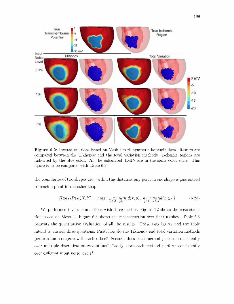
109
Figure 6.2: Inverse solutions based on Mesh 1 with synthetic ischemia data. Results are compared between the Tikhonov and the total variation methods. Ischemic regions are indicated by the blue color. All the calculated TMPs are in the same color scale. This figure is to be compared with Table 6.3.
the boundaries of two shapes are: within this distance, any point in one shape is guaranteed to reach a point in the other shape.
H a u ssD ist(X ,Y ) = max {m ax min d (x,y), max m ind(x,y) } (6.25)x€X y€Y y£Y x€X
We performed inverse simulations with three meshes. Figure 6.2 shows the reconstruc
tion based on Mesh 1. Figure 6.3 shows the reconstruction over finer meshes. Table 6.3 presents the quantitative evaluation of all the results. These two figures and the table
intend to answer three questions. First, how do the Tikhonov and total variation methods perform and compare with each other? Second, does each method perform consistently
over multiple discretization resolutions? Lastly, does each method perform consistently
over different input noise levels?
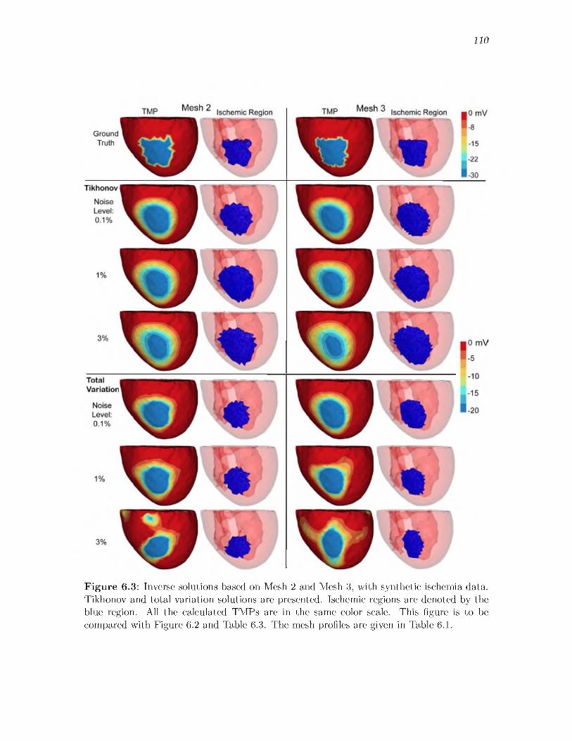
110
Figure 6.3: Inverse solutions based on Mesh 2 and Mesh 3, with synthetic ischemia data. Tikhonov and total variation solutions are presented. Ischemic regions are denoted by the blue region. All the calculated TMPs are in the same color scale. This figure is to be compared with Figure 6.2 and Table 6.3. The mesh profiles are given in Table 6.1.

111
Table 6.3: Inverse simulation with an isotropic heart model and synthetic ischemia data, over three meshes and noise levels.
Mesh Noise Correlation coefficient Centroid distance (mm) Haussdorff distance (mm)Tikhonov Total variation Tikhonov Total variation Tikhonov Total variation
0.1 % 0.78 0.69 1.2 2.0 7.1 6.6Mesh 1 1% 0.74 0.65 1.4 1.8 7.8 6.6
3% 0.68 0.37 1.0 1.9 10.3 8.00.1% 0.73 0.65 1.7 2.5 5.1 7.8
Mesh 2 1% 0.69 0.66 1.7 2.4 7.6 7.83 % 0.66 0.41 1.8 4.3 7.9 10.20.10% 0.70 0.72 0.8 2.2 5.2 5.4
Mesh 3 1% 0.68 0.60 0.9 2.7 6.8 6.23 % 0.65 0.45 0.9 3.9 7.5 13.4
Note: This table is related to Figure 6.2 and Figure 6.3.
Overall, we obtained good reconstructions of both the TMP and the ischemic region,
and the results were consistent over multiple noise levels and mesh sizes. The amplitude
of reconstructed results was roughly two-thirds of that of the ground truth, but our reconstruction achieved a high correlation, ranging from 0.7 to 0.8. The high correlation in turn resulted in a good estimation of the ischemic region: the centroid distance ranged from 1
to 3 mm, and the Haussdorff distance ranged from 5 to 10 mm.
In Figure 6.2 and Figure 6.3, the Tikhonov solutions have a smooth transition at the ischemia border zone, whereas the total variation solutions preserve a sharp transition.
Generally, the Tikhonov solutions tend to overestimate the ischemic region, whereas the
total variation solutions tend to underestimate the ischemic region. In Figure 6.3, the TMP fields from the total variation method still exhibit an ellipsoid shape at the ischemic region
(the blue region), similar to the Tikhonov solution (except being sharper than the latter).
This fact illustrates the characteristic of the fixed-point iteration: it solves a sequence of Tikhonov minimization problems.
Figure 6.3 shows that both the Tikhonov and total variation methods performed con
sistently over multiscale resolutions. Such consistency is attributed to that fact that we
formulated the optimality conditions in the continuous space before applying discretization.Table 6.3 shows that both methods performed robustly up to 1% input noise. The
Tikhonov method still performed well at 3% noise, but the total variation method started
to make significant artifacts.
6.8 .2 R ea l Ischem ia D ata w ith an A n iso tro p ic H eart M o d e lThis test was the most realistic simulation in our study. In the animal experiment,
ischemia was introduced into a perfused, live, beating canine heart by adjusting the blood

112
flow to the left anterior coronary artery, which we controlled by means of a thin glass
cannula, external blood lines, and a rotating pump. The extracellular potentials were
recorded at 1 KHz sampling rate at 247 nodes on the epicardial surface, and at 400 nodes within the ventricular myocardium (by inserting 40 fiberglass needles, each of which carrying
10 electrodes along its length). Data postprocessing included gain adjustment, baseline
adjustment, registration to the same heart geometry, and extrapolating the potentials throughout the heart volume using volumetric Laplacian interpolation. Our simulation used
the potentials at the time instant placed after the QRS complex by 40 % of the duration of
the ST interval, which was measured from the end of the QRS complex to the peak of the
T wave. At this time, the TMPs throughout the heart are believed to stay stably in the
plateau phase, and to be nearly constant in a healthy heart. We used both an anisotropic
heart model whose conductivities are given in Table 6.2 and an isotropic torso model.
It is not possible to measure TMP throughout the heart, so the verifiable ground truth is not the TMP but the extracellular potential, which we measured by means of epicardial
and intramyocardial electrodes. We first calculated the heart TMP from the measured
extracellular potential, and treated that as the true TMP. This task is a well-posed inverse problem and is fulfilled by forming another optimization problem as follows:
v = argmin\\u — u0\\l2(h), subject to Equation (4.19). (6.26)u,v
where u0 denotes the measured extracellular potential and Equation (4.19) is the bioelectric
model. In practice, the misfit ||u — u0\| is typically below 10-9 .Since we did not know the exact ischemic region, we examined the reconstructed trans
membrane and extracellular potential fields. Our examination revolved around the roles of
three simulation parameters: (1) the Tikhonov method versus the total variation method,
(2) inverse solutions under multiple scales, and (3) the impact of input noise. Table 6.4
contains full results of the Tikhonov method, and Table 6.5 for the total variation method. Figure 6.4 compares the inverse solutions by both methods. Figure 6.5 shows the inverse
solutions over multiple discretization scales.
Overall, the results of the inverse solutions were very encouraging: the reconstructed
transmembrane potential had a correlation of 0.9 with the truth, and the correlation was 0.8
in the extracellular potential. Both the Tikhonov method and the total variation method
yielded consistent inverse solutions under different discretization scales and different levels
of input noise. The Tikhonov method behaved robustly up to 3% input noise, whereas the total variation method became a little unstable at 3% noise.

113
Table 6.4: The Tikhonov inverse solutions with the anisotropic heart model and clinical ischemia data. Inverse simulation was performed over three meshes and input noise levels.
Input Mesh CC of TMP CC of EXP Number of New- CPU time per Total CPUnoise ton iteration iteration (sec) time (sec)
Mesh 1 0.93 0.83 17 325 5,5170.1% Mesh 2 0.93 0.80 17 270 4,603
Mesh 3 0.91 0.79 20 701 14,020Mesh 1 0.90 0.80 16 330 5,283
1% Mesh 2 0.91 0.78 17 265 4,506Mesh 3 0.89 0.78 18 758 13,640Mesh 1 0.90 0.79 16 329 5,256
3% Mesh 2 0.90 0.77 19 451 8,573Mesh 3 0.88 0.77 20 633 12,660
CC: the correlation coefficient between the true and computed values. TMP: the heart transmembrane potential. EXP: the heart extracellular potential.
Table 6.5: The total variation inverse solutions with the anisotropic heart model and clinical ischemia data. Inverse simulation was performed over three meshes and input noise levels.
Inputnoise
Mesh CC of TMP CC of EXP Number of fixed- point iteration
Total CPU time (sec)
Mesh 1 0.88 0.68 14 5,8120.1% Mesh 2 0.89 0.76 14 63,504
Mesh 3 0.85 0.67 12 97,283Mesh 1 0.86 0.69 10 4,024
1% Mesh 2 0.89 0.77 8 68,911Mesh 3 0.69 0.59 15 113,610Mesh 1 0.83 0.68 12 13070
3% Mesh 2 0.85 0.72 11 74,371Mesh 3 0.56 0.48 21 215,860
CC: correlation coefficient. TMP: transmembrane potential. EXP: extracellular potential.
As anticipated, the Tikhonov method yielded a smoothed solution whereas the total variation method yielded a sharper reconstruction (see Figure 6.4). The real transmem
brane potential exhibited a smooth transition at the ischemia border rather than behaving
like a stepwise function. This feature partly explains why the Tikhonov method slightly
outperformed the total variation method in terms of the correlation (see Table 6.6 and
Table 6.7). On the other hand, the total variation method seemed to better delineate the
ischemic region than did the Tikhonov.
Table 6.4 and Table 6.5 indicate that computation time can be a significant concern for the total variation method but not for the Tikhonov method. To see this, each fixed point
iteration of the total variation method is equivalent to solving a Tikhonov minimization
problem once. Throughout our tests, the number of iterations was independent of the
problem size, in both methods. However, the time each iteration took was dictated by the

114
Figure 6.4: Inverse solutions based on Mesh 1, with clinical ischemia data. Each figure shows reconstructed heart potentials at the same cross section. The figures in each column are in the same color scale. This figure is to be compared with Table 6.4 and Table 6.5.
problem size. Most implementations of the interior-point method involve an LTDL Cholesky
factorization of a symmetric positive definite matrix, whose size is dictated by the number of control variables. We conclude that Mesh 3 (~6500 nodes on heart) is an appropriate resolution for conducting the total variation method on moderate computational platforms.
6.8 .3 R ea l Ischem ia D ata w ith an Iso trop ic H eart M o d e l
This test explores whether it is possible to estimate real heart potentials with reasonable
accuracy without using anisotropic conductivities because such information is not available
in any remotely realistic clinical scenarios except by means of rule-based estimation [115].
We conducted forward simulation using the same anisotropic heart model and voltage data
as described in Section 6.8.2, and then conducted inverse simulation using the isotropic
heart model as described in Section 6.8.1.

115
Figure 6.5: Tikhonov and total variation inverse solutions based on Mesh 2 and Mesh 3, using clinical ischemia data. The reconstructed heart potentials in each column are in the same color scale. This figure is to be compared with Table 6.4 and Table 6.5.
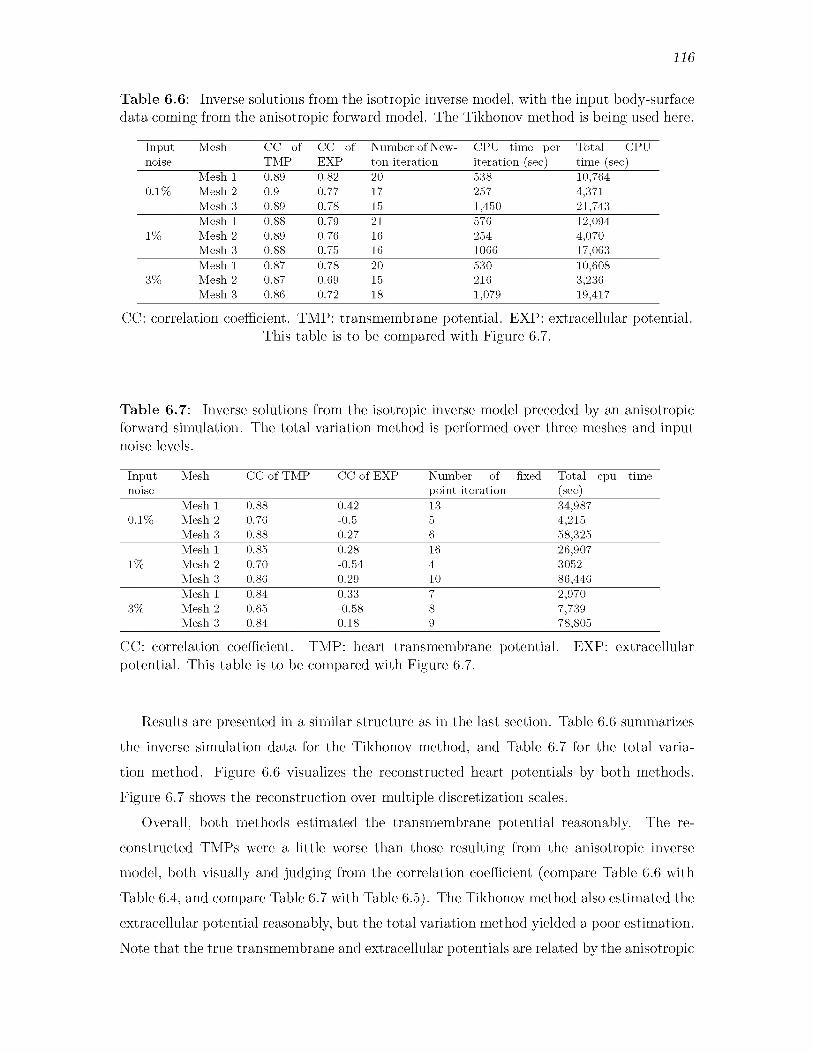
116
Table 6.6: Inverse solutions from the isotropic inverse model, with the input body-surface data coming from the anisotropic forward model. The Tikhonov method is being used here.
Input Mesh CC of CC of Number of New- CPU time per Total CPUnoise TMP EXP ton iteration iteration (sec) time (sec)
Mesh 1 0.89 0.82 20 538 10,7640.1% Mesh 2 0.9 0.77 17 257 4,371
Mesh 3 0.89 0.78 15 1,450 21,743Mesh 1 0.88 0.79 21 576 12,094
1% Mesh 2 0.89 0.76 16 254 4,070Mesh 3 0.88 0.75 16 1066 17,063Mesh 1 0.87 0.78 20 530 10,608
3% Mesh 2 0.87 0.69 15 216 3,236Mesh 3 0.86 0.72 18 1,079 19,417
CC: correlation coefficient. TMP: transmembrane potential. EXP: extracellular potential. This table is to be compared with Figure 6.7.
Table 6.7: Inverse solutions from the isotropic inverse model preceded by an anisotropic forward simulation. The total variation method is performed over three meshes and input noise levels.
Inputnoise
Mesh CC of TMP CC of EXP Number of fixed point iteration
Total cpu time(sec)
Mesh 1 0.88 0.42 13 34,9870.1% Mesh 2 0.76 -0.5 5 4,215
Mesh 3 0.88 0.27 6 58,325Mesh 1 0.85 0.28 16 26,907
1% Mesh 2 0.70 -0.54 4 3052Mesh 3 0.86 0.29 10 86,446Mesh 1 0.84 0.33 7 2,970
3% Mesh 2 0.65 -0.58 8 7,739Mesh 3 0.84 0.18 9 78,805
CC: correlation coefficient. TMP: heart transmembrane potential. EXP: extracellular potential. This table is to be compared with Figure 6.7.
Results are presented in a similar structure as in the last section. Table 6.6 summarizes
the inverse simulation data for the Tikhonov method, and Table 6.7 for the total varia
tion method. Figure 6.6 visualizes the reconstructed heart potentials by both methods.
Figure 6.7 shows the reconstruction over multiple discretization scales.Overall, both methods estimated the transmembrane potential reasonably. The re
constructed TMPs were a little worse than those resulting from the anisotropic inverse model, both visually and judging from the correlation coefficient (compare Table 6.6 with
Table 6.4, and compare Table 6.7 with Table 6.5). The Tikhonov method also estimated the extracellular potential reasonably, but the total variation method yielded a poor estimation.
Note that the true transmembrane and extracellular potentials are related by the anisotropic

117
Figure 6.6: Inverse solutions of an isotropic inverse model following an anisotropic forward simulation. Here Mesh 1 is being used. The reconstructed heart potentials in each column are in the same color scale. This figure is to be compared with Table 6.6 and Table 6.7.
model, so one should not expect to estimate both of them accurately at the same time. Our
inverse calculation treated the TMP as the “source,” so the recovered extracellular potential can be regarded as the outcome of the recovered TMP according to the isotropic model.
Over different mesh sizes and noise levels, the Tikhonov method behaved more consistently than the total variation method. The computational time was largely consistent,
except in Mesh 2, where both methods took much less time than anticipated and did not reduce the iteration number. Our inspection showed that after identifying the search
direction at each iteration, our optimization solver computed the step size faster than usual.
This fast solution might be attributed to this specific discretization.

118
Figure 6.7: Inverse solutions of the isotropic heart model following an anisotropic forward simulation, based on Mesh 2 and Mesh 3. Tikhonov and total variation methods are compared under three input noise levels. The reconstructed heart potentials in each column are in the same color scale. This figure is to be compared with Table 6.6 and Table 6.7.

119
We concluded that it is possible to estimate the TMP with reasonable accuracy without anisotropic information, and the Tikhonov is the preferred method for this reconstruction.
Anisotropy mainly influences the distribution of the extracellular potential but does not significantly impact source estimation from the body surface. One explanation is that the
attenuation and superposition effects of the torso volume overwhelms the impact of heart
anisotropy, so the latter is not a critical factor in inverse source estimation.
6.9 Discussion6.9.1 B iop h ysica l C on siderations
6.9 .1 .1 T ik h on ov versus T ota l V ariationOur experiments show that both regularization methods were able to achieve reasonable
inverse solutions, with minor differences in accuracy. The Tikhonov method performed
robustly over different discretization resolutions and input noise levels, whereas the total
variation (TV) method became unstable under the 3% noise level with high-resolution heart models (Figure 6.3). In the absence of heart conductivity information, the Tikhonov
method outperformed the TV method. The Tikhonov method was also 10-20 times faster
than the fixed-point TV method. Although the TMP in an ischemic heart (during the ST
interval) is often modeled by some smoothed variants of a step function, we found that the TMP distribution was quite smooth in real conditions, judging from our extracellular
potential (experimentally measured) and TMP (inversely calculated) shown in Figure 6.5. This finding makes the Tikhonov method more appealing than one would initially anticipate.
In summary, for the reasons detailed below, we would advocate the Tikhonov method as
both capable of achieving a clinically useful level of accuracy and computationally reasonable for estimating the TMP when localizing ischemia.
6 .9 .1 .2 B ord er Z on e C on sid erationThe ischemic border zone, which comprises progressive changes in electrophysiological
properties between the healthy and ischemic regions, characterized by a spatial transition of TMP, is of great clinical interest in ischemia studies. The spatial gradient of TMP in
the border zone results in “injury currents,” which are believed to be the primary electric
source causing the ST segment shift [74]. Therefore, the shape and width of border zones should be considered when choosing the resolution for the heart geometry. A border zone
is often estimated to be between 5-10 mm in thickness [108], and the grid size of our mesh ranged between 5 mm (Mesh 1) and 2 mm (Mesh 3) so as to represent the border zone
reasonably.

120
Our simulations indicated that the transition could be reasonably reconstructed whether
it was sharp or smooth. In our synthetic study, the border zone was set to be one-element wide (thus thinner than normal), and accordingly the synthetic TMP had a sharper tran
sition than normal. From the view of inverse problems, if a “ground truth” TMP contains
sharper transitions, it is more difficult to reconstruct. However, we found that the TV
method was able to reconstruct the sharp voltage transition in border zones (see Figure 6.3).
In our real data study, the border zone transition was smoother than in our synthetic setting,
and the Tikhonov method again yielded good recovery, as shown by Figure 6.5. (See [108] for
more discussion of the experimental ischemic voltage data we used.) These tests indicated that recovering the voltage transition in border zones should not create extra technical
difficulty to the overall goal of recovering the TMP.
6.9 .1 .3 Im p act o f T issue A n iso trop yA few simulation studies based on real ischemia data have shown that fiber rotation and
tissue anisotropy are fundamental in determining epicardial extracellular potential distri
butions and ST displacement patterns (in the sense of forward simulation) [98]. However, in clinical practice, the heart fiber information of an individual patient is generally not
available, though scientists have recently started to acquire or estimate this information
on a patient-specific basis [114]. Therefore, it is worth inquiring whether it is possible to reasonably reconstruct the myocardial TMP without the information of heart anisotropy,
while the input body-surface potentials actually result from an anisotropic heart. We
explored this possibility in Section 6.8.3. In our inverse calculation, the TMP was the
control variable whereas the extracellular potential was subject to the TMP via an isotropic
bidomain heart model. We found that without including the heart anisotropy, one still
may reconstruct the TMP with reasonable accuracy, but one would poorly estimate the extracellular potential, as shown by Figure 6.6 and Figure 6.7.
This finding not only confirms previous understanding that the heart anisotropy is
indispensable for the forward calculation, but also indicates that including the anisotropy
is less critical to the inverse calculation. For the second indication, we conjecture that
given the TMP source, the body-surface potentials are dominated by the attenuation and
superposition effect of the torso volume, so that the effect of myocardial anisotropy is
overwhelmed. Therefore, if the torso’s effect can be properly managed in the inverse
calculation (which is the main purpose of regularization), it is possible to estimate the TMP with moderate accuracy. Regarding the first indication, because the extracellular potentials
were obtained by a forward calculation based on the reconstructed TMP, the absence of

121
heart anisotropy prevents accurate estimation of the extracellular potentials. An earlier
study asserted that heart anisotropy, especially the anisotropy of the ischemic regions,
was critical in predicting extracellular epicardial potentials [51]. Our finding confirms that assertion from the reverse side (i.e., lack of anisotropy leads to poor estimation of
extracellular potentials).
6 .9 .1 .4 H igh -R eso lu tion M o d e l for Inverse S im ulationOne highlighted feature of our work is achieving accurate inverse solutions with a much
finer heart model than in previous studies. Most previous studies of inverse ECG reported
heart models of less than 1,000 nodes, whereas our model of 17,000 nodes would still
be clinically reasonable if computation resources were incrementally increased. A major
reason for choosing coarse models is to avoid worsening the ill-conditioning of the resulting
numerical system. This concern is addressed by our optimize-then-discretize approach, which enables consistent optimization performance over multiple resolutions. We advocate
this approach for inverse ECG studies because it may reveal heart conditions in more detail than has been possible to date.
6 .9.2 C om p u ta tion a l C on sideration s
6.9 .2 .1 Indiv idualized D iscretization
In this study, we used the same mesh to discretize the control variable v , the state variable u , and the adjoint variable p , but this is not necessary. Individual and adaptive discretization of each variable deserves further investigation. In inverse problems, one
often wishes to discretize the control variable v coarsely so as to exert certain projective
regularization effect, meanwhile taking a finer discretization of the state variable u [118]. The discretization concern for the adjoint variable has been discussed in Section 6.4.1. In our
problem, p does not need to stress stronger regularity than u , so the same discretization for
both is fine unless computation resource becomes a serious bottleneck. It is straightforward to incorporate individual discretization into our framework— See Equation (4.22) for the
PDE constraint and Equation (6.5) for the optimality conditions.
6 .9 .2 .2 A d a p tiv e FE R efinem ent in InversionPDE-constrained optimization is computationally intensive: the optimization procedure
is normally iterative, and each iteration needs to solve the entire PDE system, which
after discretization may amount to millions of variables. Computational efficiency can be
improved in two ways: achieving convergence with less iteration, or reducing the numerical

122
cost in each iteration. Adaptive finite element methods take effect in the latter way by discretizing PDEs differently in each optimization iteration. While adaptive finite
element refinements have been well established both in theory and in practice in solving
PDEs, they have not yet been widely adopted in PDE-constrained optimization, partly be
cause most practical optimization solutions adopt the discretize-then-optimize approach, in which discretization cannot be changed between iterations (otherwise the finite-dimensional
convergence criteria become meaningless). To achieve the adaptive refinement in PDE-
constrained optimization, one must take the optimize-then-discretize approach and then
perform refinement based on certain error estimates for finite element methods. In this
study, we have finished the foundation work of merging optimization and finite element
discretization (see Section 6.4), and we defer adaptive refinement to future work, a valuable topic that deserves extensive investigation.
6 .9 .2 .3 A d v a n ced A lgorith m s for T ota l V ariation
We implemented the TV minimization by the fixed-point iteration, a choice that is relatively robust but certainly not optimal in performance. Our intention is not to thor
oughly explore algorithms for the TV minimization, but to formulate the minimization in
the finite element context. Such formulation lays the basis upon which various advanced algorithms can be applied. Advanced algorithms tackle the TV minimization in both the
primal and dual spaces instead of the primal space alone. The primal-dual formulation
not only converges faster, but also removes the expediency of smoothing singularity points
(see e in Equation (6.10)) and hence allows one to directly pursue unsmoothed solutions. These algorithms are fully compatible with our finite element formulation and fulfilling those algorithms is a meaningful extension of our current work.
6 .9 .2 .4 Form ulation in G eneral S ob o lev SpacesWe formed the variational optimality conditions of the PDE-constrained optimization in
the L2 space, with the inner product taking equal weights between the trial and test spaces
(see Equation (4.9)). The optimality conditions can also be formed in the general Sobolev
spaces as described in the classical literatures of FEMs. A proper choice of the variational
formulation should take into account two issues: (1) the inherent structure of the given
optimization functional and PDE constraints and (2) the regularity of the finite element
solution. Reexamining the finite element theories for PDEs in the context of constrained
optimization deserves further investigation.

123
6.10 ConclusionIn this chapter, we attempted to localize myocardial ischemia by inversely computing
the myocardial transmembrane potential from body-surface potential maps. To tackle this ill-posed problem, we proposed a general PDE-constrained optimization framework whose
main features are summarized as follows:
• Formulating optimality conditions in the continuous space so as to isolate optimization and discretization;
• Tikhonov and total variation minimization seamlessly integrated with finite element
solutions;
• A tailored primal-dual method for efficiently handling inequality constraints.
By allowing one to impose various physically-based constraints, this framework obtained
promising reconstruction results even under realistic situations, indicating that our inverse solution is feasible and suitably accurate for localizing the common case of myocardial
ischemia. Finally, we believe the PDE-constrained optimization framework may benefit a
broad range of bioelectromagnetic problems in heart and brain research.

CHAPTER 7
SUMMARY
The overarching theme of this dissertation is the formulation, optimization, and solution
of the inverse ECG problem using the finite element method. The theme comprises two
main thrusts: optimal finite element discretization of the inverse problem, and a new inverse
solution method called PDE-constrained optimization. Each thrust contains two major
goals, leading to four thesis goals stated as follows:
1. Propose refinement strategies for optimal finite element discretization of the inverse ECG problem.
2. Fulfill Goal 1 by developing h/p-type finite element refinements.
3. Formulate a PDE-constrained optimization framework and its finite element solution.
4. Apply the optimization method to solve the bidomain-based inverse ECG problem for
localization of myocardial ischemia.
In Chapter 5, we addressed the first research thrust, with the main conclusion that discretization is important to the solution of the inverse problem by impacting both the
approximation accuracy and conditioning of the resulting algebraic problem. A sensible dis
cretization may achieve extra improvement of inverse solutions on top of existing inverse calculation techniques. We first demonstrated that the traditional, forward-problem-oriented refinement approach, focusing on improving the approximation accuracy alone, increases the
degree of ill-conditioning of the inverse problem, thus motivating our quest for refinement
strategies oriented to the inverse problem. Based on a Fourier analysis that quantifies how
discretization relates to ill-conditioning, we proposed a set of refinement guidelines including
the following issues: the heart surface, the torso volume, and the heart-to-volume interface.
The pursued fidelities of the heart surface largely dictate the degree of ill-conditioning and therefore, one should set the resolution of the heart surface based on one's clinical needs, but
not pursue excessive fidelities to avoid unnecessary numerical sensitivity. The fidelities of the

125
torso volume dictate how much information determined by the heart-surface fidelities can
be inversely recovered, so the torso volume needs sufficient refinement to avoid “artificial” ill-conditioning. Refinement of the heart-to-volume interface also gains benefits, as such refinement both captures the high voltage-gradient field near the heart and improves the
boundary-lifting operation of the FEM.
Regarding Goal 2 of fulfilling our refinement guidelines, we developed two finite element
refinement methods, one by spatially refining the mesh (h-type) and the other by using
high-order finite elements (p-type). One major concern in refinement is that refining the
elements near the heart without decreasing mesh size on the heart surface will cause aspect-
ratio problems for tetrahedral elements. With the h-refinement, we resolved this concern by the use of hybrid finite elements, in which we used quadrilateral (in 2D) or prismatic elements (in 3D) to decouple the refinements in the normal direction and in the tangential
direction. With the p-refinement, we resolved the above concern by extracting and using
only the linear components of the FE approximation at the heart surface. Such adapted
p-refinement, fulfilled in the polynomial space, provides a seamless solution for selective refinement in the spatial domain, and circumvents the aspect-ration problem that obstructs
h-refinement methods. The implementation of our adapted p-refinement was facilitated by our use of hierarchical, modal finite-element basis expansions. Our simulation experiments
showed that both refinement methods mitigate the ill-conditioning and improved the inverse solution. Finally, in order to make the inverse calculation consistent when the inverse
problem is discretized under multiple scales, we proposed a new family of variational-form regularizers that serve as an alternative to the classic algebraic Tikhonov regularizers.
The second research thrust, presented in Chapter 6, involves a new inverse solution
methodology that has so far seen limited use in ECG problems: PDE-constrained optimization. Our main contribution lied in the formulation and solution of a general optimization
framework that accepts convex objective functionals and allows physically-based constraints
in both equality and inequality forms. One highlighted feature of this framework was the derivation of optimality conditions in the continuous space, thereby separating optimization from discretization choice. We also derived closed-form finite element solutions for the
L2-norm Tikhonov regularization and the Li-norm total variation regularization. A typical
challenge of PDE-constrained optimization is the large scale of its resulting numerical
systems. To tackle this challenge, we fulfilled the numerical optimization by developing
a primal-dual interior-point method tailored to the specific algebraic structure of the given optimization problem and PDE constraints.

126
Regarding Goal 4, we applied our optimization methodology to localization of cardiac
ischemic disease, by inversely reconstructing the transmembrane potential throughout the
myocardium based on the bidomain heart model. Because of its difficulty, this bidomain- based inverse ECG problem has previously seen minimal progress beyond studies based
on simplified, two-dimensional settings. With our new inverse solution methodology, we
achieved promising results based on a realistic simulation using a three-dimensional, fiber-
included heart model with experimental ischemia data. One highlight of the results was
a nice recovery with a heart model of over 100,000 elements (Figure 6.5), a much finer
discretization than any heart models previous reported. Our good reconstructions were
attributed to three factors: (1) the inclusion of the whole PDE model as a constraint,
(2) the flexibility to impose various physically-based constraints, and (3) the separation of optimization from discretization. While the goal of reproducing the transmembrane
potential in general clinical cases remains exceedingly challenging, our study indicated the feasibility to make reasonable reconstruction in the case of myocardial ischemia and to
localize ischemic regions.
7.1 Future WorkBoth the inverse problems associated with PDEs in general, and the inverse problems
arising in electrocardiography in particular, remain at the frontiers in scientific computing
research. We now suggest several high-level directions in these two areas that warrant future research.
7.1.1 U n certa in ty Q uantification and Inversion
In this dissertation, we have concentrated on a deterministic approach to the inverse problem. However, uncertainty is inherent and ubiquitous in real-world inverse problems:
measurements are noisy; accurate model parameters may be unavailable; or fundamentally,
we may have insufficient knowledge of the physical system under investigation. Understanding and quantification of uncertainty in inverse problems are receiving increasing attention
in recent years. Future research on this topic may be pursued on the modeling side or the computational side.
On the modeling side, inverse problems need statistical formulation that incorporates
uncertainties and prior information in stochastic forms. Topics of interest include modeling
uncertainty, studying the propagation of uncertainty within the given physical problem, evaluating parameter sensitivity, and developing inverse solutions in stochastic settings. An
appealing prospect of the approach of a statistical inverse problem is that the problem may

127
be much better-posed than the deterministic approach. In a statistical inverse problem, the
inverse solution takes the form of a probability distribution over the space of admissible
solutions. Because the inversion task now becomes pursuing a wider space of admissible solutions rather than pursing a particular solution (which is the deterministic approach),
the inverse problem becomes much better-posed.A good start point for solving statistical inverse problems may be a Bayesian framework
that models uncertainties with some probability distribution functions and handles stochas
tic structures with sampling methods such as Monte-Carlo or polynomial-chaos [124]. In
our specific inverse problem domain, electrocardiography, the sources of uncertainty include
tissue conductivity, anatomical variance among subjects, approximation error in geometry, the movement of the heart, and measurement precision. The impact of these uncertainties
on the forward ECG problem has been explored [32], but their impact on the inverse ECG problem remains unexplored.
On the computation side, because the recovery of probability distribution is conducted in the high-dimensional parameter space, it may be computationally intractable to completely
recover probability distributions for large-scale PDE systems. There is a crucial need for the development of scalable algorithms that achieve any of the following goals: (1) resolving
the curse of dimensionality by judicious dimension reduction or surrogate approximation;
(2) improving the solutions by assimilating a growing amount of available data; in our ECG
case, the goal would be to improve cardiac source recovery by multiple measurements of
body-surface potentials; and (3) exploiting the massively parallel computing infrastructures
in the era of peta-scale computing.
7.1.2 P D E -C on stra in ed O ptim iza tion w ith A d a p tiv e P D E SolversIn this dissertation, we investigated two topics: the finite element adaptation for the
classical inverse-problem formulation involving the transfer matrix (Chapter 5), and a new
inverse solution method by PDE-constrained optimization (Chapter 6). One worthwhile
future direction is to merge these two topics, i.e., to integrate adaptive finite element PDE solvers into PDE-constrained optimization.
PDE-constrained optimization is inherently computationally intensive: Nonlinear op
timization procedure is normally iterative, and each iteration involves one solution of the
whole PDE system. An area under active research is to develop efficient integration of nonlinear optimization algorithms and adaptive PDE solvers. Such an integration contains two meanings. First, the PDEs are solved under different discretizations in each iteration.
Second, different physical quantities in the PDEs may use different quantities. Because such

128
integration is intrusive into both ends, adaptive finite elements and error estimates have not seen wide application in PDE-constrained optimization, despite their common use in
numerical solutions of PDEs.The foundation for adaptive PDE solvers in optimization is the optimize-then-discretize
approach, which we have developed in Section 6.4. An important question that remains to
be solved is the FE error estimates oriented toward the optimization procedure. The criteria for existing FE error estimates are mostly based on approximation error or smoothness of
the true PDE solution. Error estimate criteria targeting the optimization process will receive
notable scientific interest. Finally, adaptive PDE solvers for PDE-constrained optimization are not limited to the finite element method, but also apply to finite difference and finite
volume methods, e.g., see the work by [43, 44].
7.1.3 P D E -C on stra in ed O ptim iza tion for O th er B ioe le ctr ic Inverse P rob lem s
PDE-constrained optimization is a general framework applicable to a broad range of
inverse problems. In this dissertation, we applied this optimization framework to a nontra-
ditional type of inverse ECG problem: to recover myocardial TMPs during the ST interval in the case of myocardial ischemia. The promising results we obtained for this previously
intractable inverse problem demonstrate the efficacy of PDE-constrained optimization.
From an electrophysiological perspective, transmural ischemia in a single region, the clinical
situation we considered, is one of the simplest representations of cardiac diseases. A direct extension of our current work will be to localize more sophisticated ischemic scenarios such
as multiple ischemic regions, subendocardial ischemia, and intramural ischemia. It is also
worthwhile to connect inverse solutions with mechanistic ischemia studies such as [50].A more ambitious goal will be to recover the myocardial TMP over the entire cardiac
cycle. Such a recovery will be of great clinical interest for localization and monitoring of a variety of cardiac abnormalities. For example, one may infer from the recovered temporal
TMP the activation sequence of the heart, which can be used to diagnose arrhythmia or
pre-excitation pathways. However, the general-case TMPs exhibit much more complicated
distributions, in terms of both the diversity in space and the variance in time, than the
piecewise-constant TMPs in our ischemia case. Accordingly, the inverse problem may be
more difficult and one needs to design advanced spatial-temporal constraints that exploit the bioelectric prior information of the considered phenomena.
Another exciting extension of PDE-constrained optimization is to those classic inverse
ECG approaches we reviewed in Chapter 3, such as the epicardial potential approach,

129
or the activation time approach. Replacing the traditional transfer-matrix formulation,
the PDE-constrained optimization offers more flexibility for constraining intermediate or
state variables, and is therefore more likely to yield better inverse solutions. For example, when solving the activation time inverse problem, one may impose constraints on the heart
potentials or on the speed of the activation wavefront, while such constraints are unlikely to impose within the transfer-matrix-based inverse calculation. Finally, PDE-constrained
optimization may bring new insights for a broad range of bioelectromagnetic problems
arising from heart and brain research.
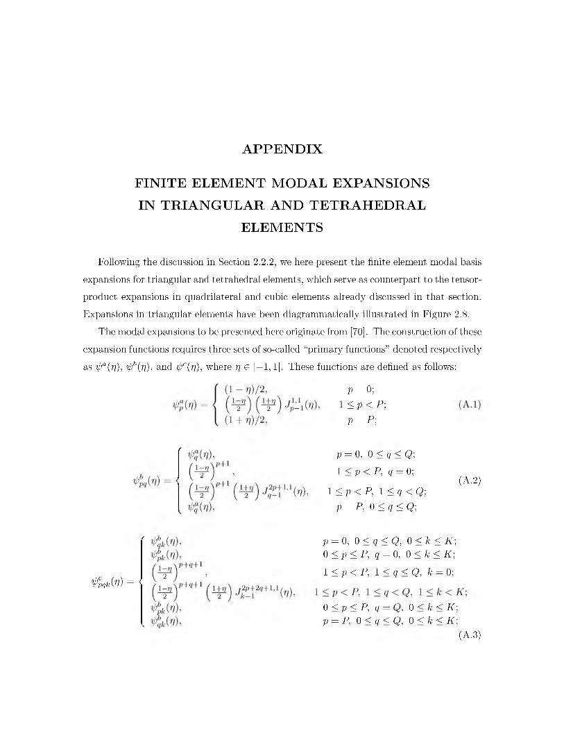
APPENDIX
FINITE ELEMENT MODAL EXPANSIONSIN TRIANGULAR AND TETRAHEDRAL
ELEMENTS
Following the discussion in Section 2.2.2, we here present the finite element modal basis
expansions for triangular and tetrahedral elements, which serve as counterpart to the tensor- product expansions in quadrilateral and cubic elements already discussed in that section.
Expansions in triangular elements have been diagrammatically illustrated in Figure 2.8.
The modal expansions to be presented here originate from [70]. The construction of these
expansion functions requires three sets of so-called “primary functions” denoted respectively
as ^ “ (n), ^b(n), and ^ c(n), where n G [-1,1]. These functions are defined as follows:
P = 0;1 < p < P ;
p = p ;
/ p = 0, 0 < q < Q;1 < p < P, q = 0;
1 < p < P, 1 < q < Q; p = P, 0 < q < Q;
(A.2)
p = 0, 0 < q < Q, 0 < k < K ;0 < p < P, q = 0, 0 < k < K ;
1 < p < P, 1 < q < Q, k = 0;pqfc (n) = <
0 < p < P, q = Q, 0 < k < K ; p = P, 0 < q < Q, 0 < k < K;
(A.3)

131
where Jp’3 (n) denotes the Jacobi polynomial. With these primary functions in place, themodal expansion functions in triangular elements, denoted by $pq( {1, { 2), are constructed in the following way:
Figure 2.8 illustrates such triangular modal expansions $pq up to the fourth order (p <
4, q < 4).The three-dimensional modal expansions are defined in a similar way using the primary
functions defined above:
• Hexahedral elements:
• Prismatic elements: &pqr (C1,C2,C3) = ^ ( ^ W ^ P r (C3)
• Pyramidic elements: ^ ( C i ,C 2,Cs)= %(m)'&Z(m)'Vpqr(ns)
• Tetrahedral elements: 0Mr(Ci, C2, C3) = ^(nOV'Pq(n2)^pqr(n3)
where n1, rf1,n2 and n3 are three-dimensional collapsed coordinates defined as follows:
$pq(Cb C2) = ^a(m )^pq(n2), - 1 < Cb 6 < 1, 6 + 6 < 0; (A.4)
(A.5)

REFERENCES
[1] 2011. SCIRun: A Scientific Computing Problem Solving Environment, Scientific Computing and Imaging Institute (SCI). Download from: http://www.scirun.org.
[2] Electrocardiography. Wikipedia, The Free Encyclopedia, Available from http://en.wikipedia.org/wiki/Electrocardiography, (accessed May 28, 2012).
[3] A h m a d , G., B r o o k s , D., a n d M a c L e o d , R. An admissible solution approach to inverse electrocardiography. Annals of Biomedical Engineering 26 (1998), 278-292.
[4] B a b u s k a , I., S t r o u b o u l i s , T., U p a d h y a y , C. S., a n d G a n g a r a j , S. K. A model study of the quality of a posteriori estimators for linear elliptic problems error estimation in the interior of patchwise uniform grids of triangles. Comput. Methods Appl. Mech. Engrg 114 (1994), 307-378.
[5] B a b u s k a , I., S t r o u b o u l i s , T., U p a d h y a y , C. S., G a n g a r a j , S. K., a n d C o p p s , K. Validation of a posteriori error estimators by a numerical approach. International Journal for Numerical Methods in Engineering 37 (1994), 1073-1123.
[6] B a n g e r t h , W. Adaptive Finite Element Methods for the Identification of Distributed Parameters in Partial Differential Equations. PhD Thesis. University of Heidelberg, 2002.
[7] B a n g e r t h , W. A framework for the adaptive finite element solution of large-scale inverse problems. SIAM J. SCI. Comput. 30, 6 (2008), 2965-2989.
[8] B a n g e r t h , W ., a n d J o s h i , A. Adaptive finite element methods for the solution of inverse problems in optical tomography. Inverse Problems 24, 3 (2008).
[9] B a r r , R. C., R a m s e y , M., a n d S p a c h , M. S. Relating epicardial to body surface potential distributions by means of transfer coefficients based on geometry measurements. IEEE Transactions on Biomedical Engineering 24, 1 (1977), 1-11.
[10] B e r r i e r , K. L., S o r e n s e n , D. C., a n d K h o u r y , D. S. Solving the inverse problem of electrocardiography using a duncan and horn formulation of the kalman filter. IEEE Transactions on Biomedical Engineering 51, 3 (2004), 507-515.
[11] B i r o s , G., a n d G h a t t a s , O. Parallel Lagrange-Newton-Krylov-Schur methods for PDE-constrained optimization. Part I: The Krylov-Schur solver. SIAM Journal of Scientific Computing 27, 2 (2005), 687-713.
[12] B i s h o p , M. J., a n d P l a n k , G. Bidomain ECG simulations using an augmented monodomain model for the cardiac source. IEEE Tran Biomed Eng 58, 8 (2011), 2297-2307.

133
[13] B i s h o p , M. J., a n d P l a n k , G. Representing cardiac bidomain bath-loading effects by an augmented monodomain approach: Application to complex ventricular models. IEEE Trans on Biomed Eng 58, 4 (2011), 1066-1075.
[14] B o y d , S., a n d V a n d e n b e r g h e , L. Convex Optimization. Cambridge University Press, 2004.
[15] B r o o k s , D., A h m a d , G., a n d M a c L e o d , R. S. Inverse electrocardiography by simultaneous imposition of multiple constraints. IEEE Trans on Biomed. Eng. 46, 1 (1999), 3-18.
[16] B u r g e r , M., M a r d a l , K.-A., a n d N ie l s e n , B. F. Stability analysis of the inverse transmembrane potential problem in electrocardiography. Inverse Problems 26 (2010).
[17] B u r n e s , J. E., T a c c a r d i , B., E r s h l e r , P. R., a n d R u d y , Y. Noninvasive electrocardiographic imaging of substrate and intramural ventricular tachycardia in infarcted hearts. Jrnl. of Amer. College of Cardio. 38 (2001), 2071-2078.
[18] B u r n e s , J. E., T a c c a r d i , B., M a c L e o d , R. S., a n d R u d y , Y. Noninvasve ECG imaging of electrophysiologically abnormal substrates in infarcted hearts : A model study. Circ. 101 (2000), 533-540.
[19] B u r n e s , J. E., T a c c a r d i , B., a n d R u d y , Y. A noninvasive imaging modality for cardiac arrhythmias. Circ. 102 (2000), 2152-2158.
[20] C h a n , T. F., G o l u b , G. H., a n d M u l e t , P. A nonlinear primal-dual method for total variation-based image restoration. SIAM Journal of Scientific Compting 20, 6 (1999), 1964-1977.
[21] C h e n g , L. K., B o d l e y , J. M., a n d P u l l a n , A. J. Comparison of potential- and activation-based formulations for the inverse problem of electrocardiology. IEEE Transactions on Biomedical Engineering 50, 1 (2003), 11-22.
[22] CIBC, 2011. Seg3D: Volumetric Image Segmentation and Visualization. Scientific Computing and Imaging Institute (SCI), Download from: http://www.seg3d.org.
[23] C u c u l i c h , p ., W a n g , Y., L i n d s a y , B., Fa d d i s , M., S c h u e s s l e r , R., RJ, J. D., L i , L., a n d R u d y , Y. Noninvasive characterization of epicardial activation in humans with diverse atrial fibrillation patterns. 1364-1372.
[24] C u c u l i c h , p ., Z h a n g , J., W a n g , Y., D e s o u z a , K., V i j a y a k u m a r , R., W o o d a r d , P., a n d R u d y , Y. The electrophysiological cardiac ventricular substrate in patients after myocardial infarction noninvasive characterization with electrocardiographic imaging. 1893-1902.
[25] C u p p e n , J. J. M. Calculating the isochrones of ventricular depolarization. SIAM Journal on Scientific and Statistical Computing 5, 1 (1984), 105-120.
[26] C u p p e n , J. J. M., a n d v a n O o s t e r o m , A. Model studies with the inversely calculated lsochrones of ventricular depolarization. IEEE Trans on Biomed Eng. 31, 10 (1984), 652-659.
[27] E l d En , L. Algorithms for the regularization of ill-conditioned least squares problems. BIT 17 (1977), 134-145.
134
[28] E n g l , H., a n d N e u b a u e r , A. Convergence rates for tikhonov regularization in finite-dimensional subspaces of hilbert scales. Proc. American Math Society 102 (1988), 587-592.
[29] E n g l , H. W ., H a n k e , M., a n d N e u b a u e r , A. Regualarization o f Inverse Problems. Kluwer, MA, 2000.
[30] F is c h e r a , G., T i l g a , B., W a c h a , P., M o d r e a , R., L e d e r b , U., a n d N o w a k , H. Application of high-order boundary elements to the electrocardiographic inverse problem. Computer Methods and Programs in Biomedicine 58, 2 (1999), 119-131.
[31] F l e t c h e r , G., F l i p s e , T., K l i g f i e l d , P., a n d M a l o u f , J. Current status of ECG stress testing. Curr Probl Cardiol 23, 7 (July 1998), 353-423.
[32] G e n e s e r , S. E. Quantification o f Stochastic Behavior in Cardiac Electrophysiological Models, vol. PhD Thesis, of School of Computing. University of Utah, 2008.
[33] G h o d r a t i , A., B r o o k s , D., T a d m o r , G., a n d M a c l e o d , R. S. Wavefront- based models for inverse electrocardiography. IEEE Trans Biomed Eng 53, 9 (2006), 1821-1831.
[34] G h o s h , S., A v a r i , J. N., R h e e , E. K., W o o d a r d , P. K., a n d R u d y , Y. Noninvasive electrocardiographic imaging (ecgi) of a univentricular heart with wolff- parkinson-white syndrome. Heart Rhythm 5, 4 (2008), 605-608.
[35] G h o s h , S., A v a r i , J. N., R h e e , E. K., W o o d a r d , P. K., a n d R u d y , Y. Noninvasive electrocardiographic imaging (ECGI) of epicardial activation before and after catheter ablation of the accessory pathway in a patient with Ebstein anomaly. Heart Rhythm 5, 6 (2008), 857-860.
[36] G h o s h , S., R h e e , E. K., A v a r i , J. N., W o o d a r d , P. K., a n d R u d y , Y. Cardiac memory in patients with Wolff-Parkinson-White syndrome: Noninvasive imaging of activation and repolarization before and after catheter ablation. Circ. 118,9 (2008), 907-915.
[37] G h o s h , S., a n d R u d y , Y. Application of l1-norm regularization to epicardial potential solution of the inverse electrocardiography problem. Annals of Biomedical Engineering 37, 5 (2009), 902-912.
[38] G r e e n s i t e , F. Some imaging parameters of the oblique dipole layer cardiac generator derivable from body surface electrical potentials. IEEE Transactions on Biomedical Engineering 39 (1992), 159-164.
[39] G r e e n s i t e , F. A new treatment of the inverse problem of multivariate analysis. Inverse Problems 18 (2002), 363-379.
[40] G r e e n s i t e , F. The temporal prior in bioelectromagnetic source imaging problems. IEEE Transactions on Biomedical Engineering 50, 10 (2003), 1152-1159.
[41] G u l r a j a n i , R. The forward and inverse problems of electrocardiography. Engineering in Medicine and Biology Magazine, IEEE 17, 5 (1998).
[42] G u l r a j a n i , R. M. Bioelectricity and biomagnetism. John Wiley & Sons Inc, 1998.

135
[43] H a b e r , E., A s c h e r , U. M., a n d O l d e n b u r g , D. On optimization techniques for solving nonlinear inverse problems. Inverse Problems 16, 5 (2000), 1263-1280.
[44] H a b e r , E., A s c h e r , U. M., a n d O l d e n b u r g , D. Inversion of 3d electromagnetic data in frequency and time domain using an inexact all-at-once approach. Geophysics 69, 5 (2004), 1216.
[45] H a n s e n , P. C. Analysis of discrete ill-posed problems by means of the l-curve. SIAM Review 34 , 4 (1992), 561-580.
[46] H a n s e n , P. C. Rank-Deficient and Discrete Ill-Posed Problems, Numerical Aspects of Linear Inversion. SIAM, Monographs on Mathematical Modeling and Computation, 1997.
[47] H e , B., L i , G., a n d Z h a n g , X. Noninvasive imaging of cardiac transmembrane potentials within three-dimensional myocardium by means of a realistic geometry anisotropic heart model. IEEE Transactions on Biomedical Engineering 50, 10 (2003), 1190-1202.
[48] H i n z e , M., P in n a u , R., U l b r i c h , M., a n d U l b r i c h , S. Analytical Background and Optimality Theory, vol. 23 of Mathematical Modelling: Theory and Applications. Springer Netherlands, 2009, pp. 1-95.
[49] H i n z e , M., P in n a u , R., U l b r i c h , M., a n d U l b r i c h , S. Discrete Concepts in PDE Constrained Optimization, vol. 23 of Mathematical Modelling: Theory and Applications. Springer Netherlands, 2009, pp. 157-232.
[50] H o p e n f e l d , B., S t i n s t r a , J. G., a n d M a c L e o d , R. S. Mechanism for ST depression associated with contiguous subendocardial ischemia. Journal of Cardiovascular Electrophysiology 15 (2004), 1200-1206.
[51] H o p e n f e l d , B., S t i n s t r a , J. G., a n d M a c L e o d , R. S. The effect of conductivity on st-segment epicardial potentials arising from subendocardial ischemia. Annals of Biomedical Engineering 33, 6 (2005), 751-763.
[52] H u i s k a m p , G. Difference formulas for the surface laplacian on a triangulated surface. Journal o f computational physics 95, 2 (1991), 477-496.
[53] H u i s k a m p , G., a n d G r e e n s i t e , F. A new method for myocardial activation imaging. Biomedical Engineering, IEEE Transactions on 44, 6 (1997), 433-446.
[54] H u i s k a m p , G., a n d v a n O o s t e r o m , A. The depolarization sequence of the human heart surface computed from measured body surface potentials. Biomedical Engineering, IEEE Transactions on 35, 12 (1988), 1047-1058.
[55] H u i s k a m p , G., a n d v a n O o s t e r o m , A. Tailored versus realistic geometry in the inverse problem of electrocardiography. IEEE Transactions on Biomedical Engineering 36, 8 (1989), 827-835.
[56] I n t i n i , A., G o l d s t e i n , R. N., J i a , P., R a m a n a t h a n , C., R y u , K., G i a n n a t t a - s i o , B., G il k e s o n , R., S t a m b l e r , B. S., B r u g a d a , P., S t e v e n s o n , W. G., R u d y , Y., a n d W a l d o , A. L. Electrocardiographic imaging (ECGI), a novel diagnostic modality used for mapping of focal left ventricular tachycardia in a young athlete. Heart Rhythm 2, 11 (2005), 1250-1252.

136
[57] I s a k o v , V. Inverse Problems for Partial Differential Equations. Springer, New York, 2006.
[58] J i a , p ., R a m a n a t h a n , C., G h a n e m , R. N., R y u , K., V a r m a , N., a n d R u d y , Y. Electrocardiographic imaging of cardiac resynchronization therapy in heart failure: observation of variable electrophysiologic responses. Heart Rhythm 3, 3 (2006), 296310.
[59] J i a n g , Y., Q i a n , C., H a n n a , R., Fa r i n a , D., a n d D o s s e l , O. Optimization of the electrode positions of multichannel ECG for the reconstruction of ischemic areas by solving the inverse electrocardiographic problem. International Journal of Bioelectromagnetism 11, 1 (2009), 27-37.
[60] J o h n s o n , C. R. Adaptive Finite Element and Local Regularization Methods for the Inverse ECG Problem. Advances in Computational Biomedicine. WIT Press, 2001.
[61] J o h n s o n , C. R., a n d M a c L e o d , R. S. Computational medicine: Bioelectric field problems. Computer 26, 10 (1993), 59-67.
[62] J o h n s o n , C. R., a n d M a c L e o d , R. S. Nonuniform spatial mesh adaptation using a posteriori error estimates: applications to forward and inverse problems. Applied Numerical Mathematics 14 (1994), 311-326.
[63] J o h n s o n , C. R., a n d M a c L e o d , R. S. Adaptive local regularization methods for the inverse ecg problem. Progress in biophysics and molecular biology 69, 2-3 (1998), 405-423.
[64] J o h n s o n , C. R., M a c L e o d , R. S., a n d M a t h e s o n , M. A. Computer simulations reveal complexity of electrical activity in the human thorax. Comp. in Physics 6, 3 (1992), 230-237.
[65] J o h n s o n , C. R., M a c L e o d , R. S., P a r k e r , S. G., a n d W e i n s t e in , D. M. Biomedical computing and visualization software environments. Communications of the ACM 47, 11 (2004), 64-71.
[66] J o h n s o n , C. R., M o h r , M., R u d e , U., S a m s o n o v , A., a n d Z y p , K. Multilevel methods for inverse bioelelectric field problems. Springer-Verlag Publishing, 2001.
[67] J o h n s t o n , P. R., a n d G u l r a j a n i , R. M. A comparison of methods for regularisa- tion parameter determination in the inverse problem of electrocardiography. Advances in Computational Bioengineering. WIT Press, 2001, pp. 191-227.
[68] K a i p i o , J., a n d S o m e r s a l o , E. Statistical and Computational Inverse Problems. Springer, New York, 2004.
[69] K a i p i o , J., a n d S o m e r s a l o , E. Statistical inverse problems: discretization, model reduction and inverse crimes. Journal of Computational Applied Math 198, 2 (2007), 493-504.
[70] K a r n i a d a k i s , G. E., a n d S h e r w in , S. P. Spectral/hp Element Methods for CFD. Oxford University Press, Oxford, UK, 1999.
[71] K h o u r y , D. S. Use of current density in regularization of the invers problem of electrocardiography. In Proc. 16th Intl. Conf. IEEE EMBS, vol. 3-6, pp. 133-134.

137
[72] K i r s c h , A. An Introduction to the Mathematical Theory of Inverse Problems. Springer, New York, 1996.
[73] L a s a n e n , S., a n d R o in in e n , L. Statistical inversion with Green’s priors. In 5th International Conference on Inverse Problems in Engineering: Theory and Practice.
[74] L i , D., L i , C. Y ., Y o n g , A. C., a n d K i l p a t r i c k , D. Source of electrocardiographic st changes in subendocardial ischemia. Circ. Res. 82 (1998), 957-970.
[75] L i u , Z., L i u , C., a n d H e , B. Noninvasive reconstruction of three-dimensional ventricular activation sequence from the inverse solution of distributed equivalent current density. Medical Imaging, IEEE Transactions on 25, 10 (2006), 1307-1318.
[76] M a c L a c h l a n , M. C., S u n d n e s , J., S k a v h a u g , O., L y s a k e r , M., N ie l s e n , B. F., a n d T v e i t o , A. A linear system of partial differential equations modeling the resting potential of a heart with regional ischemia. Math. Biosci. 210, 1 (2007), 238-252.
[77] M a c L e o d , R., a n d B r o o k s , D. Recent progress in inverse problems in electrocardiology. IEEE Eng Med Biol Mag 17, 1 (1998), 73-83.
[78] M a c L e o d , R., J o h n s o n , C., a n d E r s h l e r , P. Construction of an inhomogeneous model of the human torso for use in computational electrocardiography. IEEE Press, pp. 688-689.
[79] M a c L e o d , R. S., T a c c a r d i , B., a n d L u x , R. L. Electrocardiographic mapping in a realistic torso tank preparation, 1995.
[80] M a l m i v u o , J., a n d P l o n s e y , R. Bioelectromagnetism. Oxford University Press, New York, 1995.
[81] M a t h e , P., a n d P e r e v e r z e v , S. V. Optimal discretization of inverse problems in hilbert scales. regularization and self-regularization of projection methods. SIAM J. Numer. Anal. 38, 6 (2001), 1999-2021.
[82] M e s s n a r z , B., S e g e r , M., M o d r e , R., F i s c h e r , G., H a n s e r , F., a n d T i l g , B. A comparison of noninvasive reconstruction of epicardial versus transmembrane potentials in consideration of the null space. IEEE Trans Biomed Eng 51, 9 (2004), 1609-1618.
[83] M e s s n a r z , B., T i l g , B., M o d r e , R., F i s c h e r , G., a n d H a n s e r , F. A new spatiotemporal regularization approach for reconstruction of cardiac transmembrane potential patterns. IEEE Trans Biomed Eng 51, 2 (2004), 273-281.
[84] N a r a , T., a n d A n d o , S. A projective method for an inverse source problem of the poisson equation. Inverse Problems 19 (2003), 355-369.
[85] N ie l s e n , B. F., C a i , X., a n d Ly s a k e r , M. On the possibility for computing the transmembrane potential in the heart with a one shot method: An inverse problem. Math Bioscience 210, 2 (2007), 523-553.
[86] N ie l s e n , B. F., Ly s a k e r , M., a n d T v e i t o , A. On the use of the resting potential and level set methods for identifying ischemic heart disease: An inverse problem. Journal o f computational physics 220, 2 (2007), 772-790.

138
[87] O h e , T., a n d O h n a k a , K. A precise estimation method for locations in an inverse logarithmic potential problem for point mass models. Appl. Math. Modelling 18 (1994), 446-452.
[88] O h e , T., a n d O h n a k a , K. An estimation method for the number of point masses in an inverse logarithmic potential problem using discrete fourier transform. Appl. Math. Modelling 19 (1995), 429-436.
[89] O s t e r , H., a n d R u d y , Y. The use of temporal information in the regularization of the inverse problem of electrocardiography. IEEE Transactions on Biomedical Engineering 39 (1992), 65-75.
[90] P e t e r , R. J., S t e p h e n , J. W., J a r i , A. K. H., a n d D a v i d , K. Inverse electrocardiographic transformations: dependence on the number of epicardial regions and body surface data points. Math Bioscience 120 (1994), 165-187.
[91] P o t s e , M., D u b e , B., R i c h e r , J., V i n e t , A., a n d G u l r a j a n i , R. M. A comparison of monodomain and bidomain reaction-diffusion models for action potential propagation in the human heart. IEEE Transactions on Biomedical Engineering 53, 12 (2006), 2425-2435.
[92] P u l l a n , A., C h e n g , L., N a s h , M., G h o d r a t i , A., M a c L e o d , R., a n d B r o o k s , D. The Inverse Problem of Electrocardiography. Springer London, 2011, ch. 9, pp. 299-344.
[93] P u l l a n , A. J., a n d B r a d l e y , C. P. A coupled cubic hermite finite element/boundary element procedure for electrocardiographic problems. Computational Mechanics 18, 5 (1996), 356-368.
[94] P u n s k e , B., N i , Q., a n d a l , e . Spatial methods of epicardial activation time determination in normal hearts. Annals of Biomed Eng 31 (2003), 781-792.
[95] R a m a n a t h a n , C., G h a n e m , R., J i a , P., R y u , K., a n d R u d y , Y. Electrocardiographic imaging (ECGI): A noninvasive imaging modality for cardiac electrophysiology and arrhythmia” . Nature Medicine 10 (2004), 422-428.
[96] R a m a n a t h a n , C., J i a , P., G h a n e m , R., C a l v e t t i , D., a n d R u d y , Y. Noninvasive electrocardiographic imaging (ecgi): Application of the generalized minimal residual (gmres) method. Annals of Biomedical Engineering 31 (2003), 981-994.
[97] R a m a n a t h a n , C., J i a , P., G h a n e m , R., R y u , K., a n d R u d y , Y. Activation and repolarization of the normal human heart under complete physiological conditions. Proc. Natational Academy of Science, U.S. (PNAS) 103 (2006), 6309-6314.
[98] R o d r i g u e z , B., T r a y a n o v a , N., a n d N o b l e , D. Modeling cardiac ischemia. Annals of the New York Academy o f Sciences 1080, 1 (2006), 395-414.
[99] R u d y , Y. From Genes and Molecules to Organs and Organisms: Heart, vol. 9. Academic Press, Oxford, 2012, pp. 268-327.
[100] R u u d , T. S., N ie l s e n , B. F., Ly s a k e r , M., a n d S u n d n e s , J. A computationally efficient method for determining the size and location of myocardial ischemia. IEEE Transactions on Biomedical Engineering 56, 2 (2009), 263 - 272.
139
[101] S c h m i d t , J. A., J o h n s o n , C. R., E a s o n , J. C., a n d M a c L e o d , R. S. Applications o f automatic mesh generation and adaptive methods in computational medicine. Springer-Verlag, 1995, pp. 367-390.
[102] S h e w c h u k , J. R. What is a good linear finite element? interpolation, conditioning, anisotropy, and quality measures. International Meshing Roundtable (2002).
[103] S h o u , G., X i a , L., M .J i a n g , F .L i u , a n d S .C r o z i e r . Forward and inverse solutions of electrocardiography problem using an adaptive bem method. FIMH LNCS 4466 (2007), 290-299.
[104] S k i p a , O. Linear inverse problem of electrocardiography: Epicardial potentials and Transmembrane voltages. PhD thesis, University Karlsruhe., 2004.
[105] S k i p a , O., N a l b a c h , M., Sa c h s e , F., C .W e r n e r , a n d O .D o s s e l . Transmembrane potential reconstruction in anisotropic heart model. International Journal of Bioelectromagnetism 4, 2 (2002), 17-18.
[106] S t e r n , S. State of the art in stress testing and ischaemia monitoring. Card Electrophysiol Rev 6, 3 (Sept. 2002), 204-208.
[107] S t i n s t r a , J. G., H o p e n f e l d , B., a n d M a c L e o d , R. S. On the passive cardiac conductivity. Annals of Biomedical Engineering 33, 12 (2005), 1743-1751.
[108] S w e n s o n , D. J., A r a s , K. K., B u r t o n , B. M., a n d M a c L e o d , R. S. Evaluation the electrical border zone approximation with subject specific ischemia models. Journal o f Cardiovascular Electrophysiology under review (2012).
[109] T h r o n e , R. D., a n d O l s o n , L. G. A comparison of spatial regularization with zero and first order tikhonov regularization for the inverse problem of electrocardiography. Computers in Cardiology 27 (2000), 493-496.
[110] T i k h o n o v , A. N., a n d A r s e n in , V. Y. Solutions of ill-posed problems. V.H. Winston & Sons, Washington D.C., 1977.
[111] T i k h o n o v , A. N., G o n c h a r s k y , A. V., S t e p a n o v , V. V., a n d Y a g o l a , A. G. Numerical Methods for the Solutin of Ill-Posed Problems. Kluwer Academic Publishers, Dordrecht, 1995.
[112] T o h , K., T o d d , M., a n d T u t u n c u , R. SDPT3—a Matlab software package for semidefinite programming. Optimization Methods and Software 11 (1999), 545-581.
[113] T o h , K., T o d d , M., a n d T u t u n c u , R. On the implementation and usage of SDPT3—a Matlab software package for semidefinite-quadratic-linear programming, Version 4.0, 2010.
[114] V a d a k k u m p a d a n , F., A r e v a l o , H., C e r i t o g l u , C., M i l l e r , M., a n d T r a y a n o v a , N. Image-based estimation of ventricular fiber orientations for personalized modeling of cardiac electrophysiology. IEEE Transactions on Medical Imaging ePub Ahead of Print (2012).
[115] V a d a k k u m p a d a n , F., A r e v a l o , H., P r a s s l , A., C h e n , J., K i c k i n g e r , F., K o h l , P., P l a n k , G., a n d T r a y a n o v a , N. Image-based models of cardiac structure in health and disease. WIREs Syst Biol Med 2, 4 (2010), 489-506.

140
[116] V i g m o n d , E. J., W e b e r d o s Sa n t o s , R., P r a s s l , A. J., D e o , M., a n d P l a n k , G. Solvers for the cardiac bidomain equations. Progress in Biophysics and Molecular Biology 96, 1-3 (2008), 3-18.
[117] V o g e l , C. R., a n d O m a n , M. E. Iterative methods for total variation denoising. SIAM Journal o f Scientific Compting 17,1 (1996), 227-238.
[118] W a n g , D., K i r b y , R. M., a n d J o h n s o n , C. R. Resolution strategies for the finite-element-based solution of the ECG inverse problem. IEEE Trans Biomed Eng 57, 2 (2010), 220-237.
[119] W a n g , D., K i r b y , R. M., a n d J o h n s o n , C. R. Finite-element-based discreitzation and regularization strategies for 3D inverse electrocardiography. IEEE Transactions on Biomedical Engineering 58, 6 (2011), 1827-1838.
[120] W a n g , Y., C u c u l i c h , p ., Z h a n g , J., D e s o u z a , K., V i j a y a k u m a r , R., C h e n , J., Fa d d i s , M., L i n d s a y , B., S m i t h , T., a n d R u d y , Y. Noninvasive elec- troanatomic mapping of human ventricular arrhythmias with electrocardiographic imaging. Sci Transl Med 3, 98 (Aug 2011), 98ra84.
[121] W a n g , Y., L i , L., C u c u l i c h , P., a n d R u d y , Y. Electrocardiographic imaging of ventricular bigeminy in a human subject. 74-75.
[122] W a n g , Y., a n d R u d y , Y. Electrocardiographic imaging of normal human atrial repolarization. 582-583.
[123] W a n g , Y., S c h u e s s l e r , R., D a m i a n o , R., W o o d a r d , p ., a n d R u d y , Y. Noninvasive electrocardiographic imaging (ecgi) of scar-related atypical atrial flutter. 1565-1567.
[124] X i u , D. Fast numerical methods for stochastic computations: A review. Communications in Computational Physics 5, 2-4 (2009), 242-272.
[125] Y a m a s h i t a , Y. Theoretical studies on the inverse problem in electrocardiography and the uniqueness of the solution. Journal of Biomedical Engineering 29 (1982), 719-725.
[126] Z h a n g , Y., G h o d r a t i , A., a n d B r o o k s , D. H. An analytical comparison of three spatio-temporal regularization methods for dynamic linear inverse problems in a common statistical framework. Inverse Problems 21 (2005), 357-382.
[127] Z h u , M., a n d C h a n , T. An efficient primal-dual hybrid gradient algorithm for total variation image restoration. Tech. rep., Dept of Math, University of California, Los Angeles, 2008.
[128] Z h u , M., W r i g h t , S., a n d C h a n , T. Duality-based algorithms for total-variation- regularized image restoration. Computational Optimization and Applications 47, 3 (2010), 377-400.


