
HIGH PERFORMANCE, BAYESIAN‐BASED PHYLOGENETIC INFERENCE FRAMEWORK
By
Xizhou Feng
Bachelor of Engineering
China Textile University, 1993
Master of Science Tsinghua University, 1996
————————————————————————
Submitted in Partial Fulfillment of the Requirements
for the Degree of Doctor Philosophy in the
Department of Computer Science and Engineering
College of Engineering and Information Technology
University of South Carolina
2006
Major Professor Chairman, Examining Committee
Committee Member Committee Member
Committee Member Dean of The Graduate School

ii
Dedication
To Rong, Kevin and Katherine

iii
Acknowledgements
During the course of my graduate study, I have been fortunate to receive advice, support,
and encouragement from many people. Foremost is the debt of gratitude that I owe to my
thesis advisors, Professor Duncan A. Buell and Professor Kirk W. Cameron. Not only
was Duncan responsible for introducing me to this interesting and fruitful field, he also
provided me inspiring guidance, great patience, and never-ending encouragement during
the past several years. I especially thank Professor Kirk W. Cameron for his invaluable
mentoring, insightful advising, and constant investing. Kirk guided me into the exciting
field of systems study, and provided opportunities and support to conduct quality
research work in several cutting-edge areas.
I thank Professor Manton Matthews for his years of academic advising and being on
my advisory committee. His guidance and support made it possible for me to explore
various fields in computer science and engineering.
I thank Professor John R. Rose and Professor Peter Waddell for their valuable
suggestions in this research work. The discussions and collaborative work with John and
Peter generated some important ideas which have been included in this thesis.
I appreciate Professor Austin L. Hughes for being on my advisory committee and
providing me critical opinions which led me to rethink and significantly improvement
this dissertation.
I also thank the faculty and staff in the Department of Computer and Engineering for
providing me one of the most wonderful training programs in the world.

iv
Finally, I thank my family for their love and support during the hard time of
completing my dissertation.
This dissertation is dedicated to my wife Rong, my son Kevin, and my daughter
Katherine.

v
Abstract
Comparative analyses of biological data rely on a phylogenetic tree that describes the
evolutionary relationship of the organisms studied. By combining the Markov Chain
Monte Carlo (MCMC) method with likelihood-based assessment of phylogenies,
Bayesian phylogenetic inferences incorporate complex statistical models into the process
of phylogenetic tree estimation. This combination can be used to address a number of
complex questions in evolutionary biology. However, Bayesian analyses are
computationally expensive because they almost invariably require high dimensional
integrations over unknown parameters. Thoroughly investigating and exploiting the
power of the Bayesian approach requires a high performance computing framework.
Otherwise one cannot tackle the computational challenges of Bayesian phylogenetic
inference for large phylogeny problems.
This dissertation extended existing Bayesian phylogenetic inference framework in
three aspects: 1) Exploring various strategies to improve the performance of the MCMC
sampling method; 2) Developing high performance, parallel algorithms for Bayesian
phylogenetic inference; and 3) Combining data uncertainty and model uncertainty in
Bayesian phylogenetic inference. We implemented all these extensions in PBPI, a
software package for parallel Bayesian phylogenetic inference.
We validated the PBPI implementation using simulation study, a common method
used in phylogenetics and other scientific disciplines. The simulation results showed that
PBPI can estimate the model trees accurately given sufficient number of sequences and
correct models.

vi
We evaluated the computational speed of PBPI using simulated datasets on a
Terascale computing facility and observed significantly performance improvement. On a
single processor, PBPI ran up to 19 times faster than the current leading Bayesian
phylogenetic inference program with the same quality output. On 64 processors, PBPI
achieved 46 times parallel speedup in average. Combining both sequential improvement
and parallel computation, PBPI can speedup current Bayesian phylogenetic inferences up
to 870 times.
.

vii
Table of Contents
Dedication ........................................................................................................................... ii
Acknowledgements............................................................................................................ iii
Abstract ............................................................................................................................... v
List of Tables ................................................................................................................... xiii
List of Figures .................................................................................................................. xiv
Chapter 1 Introduction ........................................................................................................ 1
1.1 Phylogeny and its applications.................................................................................. 1
1.2 Phylogenetic inference.............................................................................................. 2
1.3 The challenges .......................................................................................................... 5
1.3.1 Searching a complex tree space ......................................................................... 5
1.3.2 Developing realistic evolutionary models ......................................................... 6
1.3.3 Dealing with incomplete and unequal data distribution .................................... 7
1.3.4 Resolving conflicts among different methods and data sources........................ 8
1.4 Bayesian phylogenetic inference and its issues ........................................................ 8
1.5 Motivation............................................................................................................... 10
1.6 Research objectives and contributions.................................................................... 11
1.7 Organization of this dissertation ............................................................................. 12
Chapter 2 Background ...................................................................................................... 14
2.1 Representations of phylogenetic trees .................................................................... 14
2.2 Methods for phylogenetic inference ....................................................................... 19

viii
2.2.1 Sequenced-based methods and genome-based methods.................................. 19
2.2.2 Distance-, MP-, ML- and BP-based methods .................................................. 20
2.2.3 Tree search strategies....................................................................................... 21
2.3 High performance computing phylogenetic inference methods ............................. 22
2.4 Bayesian phylogenetic inference ............................................................................ 23
2.4.1 Introduction...................................................................................................... 23
2.4.2 The Bayesian framework ................................................................................. 25
2.4.3 Components of Bayesian phylogenetic inference............................................ 27
2.4.4 Likelihood, prior and posterior probability...................................................... 27
2.4.5 Empirical and hierarchical Bayesian analysis.................................................. 28
2.5 Models of molecular evolution ............................................................................... 29
2.5.1 The substitute rate matrix................................................................................. 29
2.5.2 Properties of the substitution rate matrix ......................................................... 31
2.5.3 The general time reversible (GTR) model ....................................................... 32
2.5.4 Rate heterogeneity among different sites......................................................... 34
2.5.5 Other more realistic evolutionary models........................................................ 35
2.6 Likelihood function and its evaluation ................................................................... 35
2.6.1 The likelihood function.................................................................................... 35
2.6.2 Felsenstein’s algorithm for likelihood evaluation............................................ 37
2.7 Optimizations of likelihood computation ............................................................... 39
2.7.1 Sequence packing............................................................................................. 39
2.7.2 Likelihood local update.................................................................................... 39
2.7.3 Tree balance ..................................................................................................... 41

ix
2.8 Markov Chain Monte Carlo methods ..................................................................... 41
2.8.1 The Metropolis-Hasting algorithm .................................................................. 41
2.8.2 Exploring the posterior distribution ................................................................. 43
2.8.3 The issues......................................................................................................... 44
2.9 Summary of the posterior distribution .................................................................... 46
2.9.1 Summary of the phylogenetic trees.................................................................. 46
2.9.2 Summary of the model parameters .................................................................. 46
2.10 Chapter summary .................................................................................................. 47
Chapter 3 Improved Monte Carlo Strategies .................................................................... 49
3.1 Introduction............................................................................................................. 49
3.2 Observations ........................................................................................................... 50
3.3 Strategy #1: reducing stickiness using variable proposal step length..................... 53
3.4 Strategy #2: reducing sampling intervals using multipoint MCMC....................... 55
3.5 Strategy #3: improving mixing rate with parallel tempering.................................. 57
3.6 Proposal algorithms for phylogenetic models......................................................... 60
3.6.1 Basic tree mutation operators........................................................................... 61
3.6.2 Basic tree branch length proposal methods ..................................................... 62
3.6.3 Propose new parameters .................................................................................. 63
3.6.4 Co-propose topology and branch length .......................................................... 63
3.7 Extended proposal algorithms for phylogenetic models......................................... 63
3.7.1 Extended tree mutation operator...................................................................... 64
3.7.2 Multiple-tree-merge operator........................................................................... 64
3.7.3 Backbone-slide-and-slide operator .................................................................. 65

x
3.8 Chapter summary .................................................................................................... 66
Chapter 4 Parallel Bayesian Phylogenetic Inference ........................................................ 68
4.1 The need for parallel Bayesian phylogenetic inference.......................................... 68
4.2 TAPS: a tree-based abstraction of parallel system ................................................. 69
4.3 Performance models for parallel algorithms........................................................... 71
4.4 Concurrencies in Bayesian phylogenetic inference ................................................ 74
4.5 Issues of parallel Bayesian phylogenetic inference ................................................ 75
4.6 Parallel algorithms for Bayesian phylogenetic inference ....................................... 77
4.6.1 Task decomposition and assignment ............................................................... 77
4.6.2 Synchronization and communication............................................................... 79
4.6.3 Load balancing................................................................................................. 80
4.6.4 Symmetric MCMC algorithm.......................................................................... 80
4.6.5 Asymmetric MCMC algorithm........................................................................ 83
4.7 Justifying the correctness of the parallel algorithms............................................... 83
4.8 Chapter summary .................................................................................................... 84
Chapter 5 Validation and Verification.............................................................................. 86
5.1 Introduction............................................................................................................. 86
5.2 Experimental methodology..................................................................................... 89
5.2.1 The model trees................................................................................................ 89
5.2.2 The simulated datasets ..................................................................................... 90
5.2.3 The accuracy metrics ....................................................................................... 90
5.2.4 Tested programs and their run configurations ................................................. 92
5.2.5 The computing platforms................................................................................. 93

xi
5.3 Results on model tree FUSO024............................................................................. 94
5.3.1 The overall accuracy of results ........................................................................ 94
5.3.2 Further analysis................................................................................................ 96
5.3.3 PBPI stability ................................................................................................. 100
5.4 Results on model tree BURK050.......................................................................... 103
5.5 Chapter summary .................................................................................................. 105
Chapter 6 Performance Evaluation ................................................................................. 107
6.1 Introduction........................................................................................................... 107
6.2 Experimental methodology................................................................................... 108
6.3 The sequential performance of PBPI .................................................................... 110
6.3.1 The execution time of PBPI and MrBayes .................................................... 110
6.3.2 The quality of the tree samples drawn by PBPI............................................. 111
6.3.3 The execution time of PBPI and MrBayes .................................................... 112
6.4 Parallel speedup for fixed problem size................................................................ 115
6.5 Scalability analysis................................................................................................ 119
6.6 Parallel speedup with scaled workload ................................................................. 121
6.6.1 Scalability with different problem sizes ........................................................ 121
6.6.2 Scalability with the number of chains............................................................ 122
6.7 Chapter summary .................................................................................................. 123
Chapter 7 Summary and Future Work ............................................................................ 124
7.1 The big picture ...................................................................................................... 124
7.2 Future work........................................................................................................... 127

xii
Bibliography ................................................................................................................... 129
.

xiii
List of Tables
Table 1 - 1: The number of unrooted bifurcating trees as a function of taxa ..................... 5
Table 5 - 1: The four model trees used in experiments..................................................... 89
Table 5 - 2: PBPI run configurations for validation and verification ............................... 95
Table 5 - 3: The number of datasets where the model tree FUSO024 is found in the
maximum probability tree, the 95% credible set of trees and the 50% majority
consensus tree. A total of 5 datasets are used in each case................................... 96
Table 5 - 4: The average distances between the model tree FUSO024 and the maximum
probability tree, the 95% credible set of trees and the 50% majority consensus tree.
A total of 5 datasets are used in each case. ........................................................... 96
Table 5 - 5: The topological distances between the model tree FUSO024 and the
maximum probability tree, the 95% credible set of trees and the 50% majority
consensus tree for datasets with 10,000 characters. Datasets are simulated under
the JC69 model. .................................................................................................... 97
Table 5 - 6: The average distances between the model tree BURK050 and the maximum
probability tree, the 95% credible set of tree and the 50% majority consensus tree.
A total of 5 datasets were used in each case. ...................................................... 103
Table 6 - 1: Benchmark dataset used in the evaluation .................................................. 109
Table 6 - 2: Sequential execution time of PBPI and MrBayes ....................................... 110

xiv
List of Figures
Figure 1 - 1: The procedure of a phylogenetic inference.................................................... 4
Figure 2 - 1: Phylogenetic trees of 12 primates mitochondrial DNA sequences.............. 15
Figure 2 - 2: The NEWICK representation of the primate phylogenetic tree................... 16
Figure 2 - 3: The nontrivial bipartitions of the primate phylogenetic tree........................ 17
Figure 2 - 4: A phylogenetic tree with support values for each clade ............................. 18
Figure 2 - 5: The transition diagram and transition matrix of nucleotides ....................... 30
Figure 2 - 6: The Felsenstein algorithm for likelihood evaluation .................................. 38
Figure 2 - 7: Illustration of likelihood local update .......................................................... 40
Figure 2 - 8: The tree-balance algorithm .......................................................................... 41
Figure 2 - 9: Metropolis-Hasting algorithm...................................................................... 42
Figure 3 - 1: A target distribution with three modes......................................................... 50
Figure 3 - 2: Distribution approximated using Metropolis MCMC methods ................... 51
Figure 3 - 3: Samples drawn using Metropolis MCMC method ...................................... 52
Figure 3 - 4: Illustration of state moves ............................................................................ 54
Figure 3 - 5: Approximated distribution using variable step length MCMC.................... 55
Figure 3 - 6: The multipoint MCMC ................................................................................ 56
Figure 3 - 7: A family of tempered distributions with different temperatures................. 58
Figure 3 - 8: The Metropolis-coupled MCMC algorithm................................................. 59
Figure 3 - 9: The extended-tree-mutation method ........................................................... 64
Figure 3 - 10: The multiple-tree-merge method ............................................................... 65
Figure 3 - 11: The backbone slide and scale method........................................................ 66

xv
Figure 4 - 1: An illustration of TAPS ............................................................................... 70
Figure 4 - 2: Speedup under fixed workload .................................................................... 73
Figure 4 - 3: The procedure of a generic Bayesian phylogenetic inference ..................... 75
Figure 4 - 4: Map 8 chains to a 4 x 4 grid, where the length each sequence is 2000 ....... 78
Figure 4 - 5: The symmetric parallel MCMC algorithm................................................... 82
Figure 5 - 1: The procedure of a simulation method for accuracy assessment................. 88
Figure 5 - 2: Run configuration for MrBayes ................................................................... 93
Figure 5 - 3: The phylogram of the model tree FUSO024................................................ 98
Figure 5 - 4: The MPP tree estimated from dataset fuso024_L10000_jc69_D001 ...... 99
Figure 5 - 5: Estimation variances in 10 individual runs ................................................ 100
Figure 5 - 6: The phylogram of the model tree BURK050............................................. 101
Figure 5 - 7: The MPP tree estimated from dataset burk050_L10000_jc69_D001.nex. 102
Figure 5 - 8: The posterior distribution of the top 50 most probable trees ..................... 104
Figure 5 - 9: The topological distances distribution of the top 50 most probable trees.. 105
Figure 6 - 1: Different speedup values computed by wall clock time and user time...... 108
Figure 6 - 2: Log likelihood plot of the tree samples drawn by PBPI and MrBayes...... 111
Figure 6 - 3: The consensus tree estimated by PBPI ...................................................... 113
Figure 6 - 4: The consensus tree estimated by MrBayes ................................................ 114
Figure 6 - 5: Parallel speedup of PBPI for dataset FUSO024_L10000 ......................... 116
Figure 6 - 6: Parallel speedup of PBPI for dataset ARCH107_L1000 ........................... 117
Figure 6 - 7: Parallel speedup of PBPI for dataset BACK218_L10000 ......................... 117
Figure 6 - 8: The consensus tree estimated by PBPI on 64 processors........................... 118
Figure 6 - 9: Parallel speedup with different number of taxa ......................................... 122

xvi

1
Chapter 1
Introduction
1.1 Phylogeny and its applications
All life on the earth, both present and past, are believed to be descended from a common
ancestor. The descending pattern or evolutionary relationship among species or
organisms, or the relatedness of their genes, is usually described by a phylogeny, a tree or
network structure, with edge length representing the evolutionary divergence along
different lineages. In a phylogeny, all existing organisms are placed on its “leaves” and
ancestral organisms are placed at its “branches,” or internal nodes.
Since all biological phenomena are the result of evolution, most biological studies
have to be conducted in the light of evolution and require information on phylogeny to
interpret data [1]. Thus, phylogenies play important roles not only in evolutionary
biology, genetics and genomics, but also in modern pharmaceutical research, drug
discovery, agricultural plant improvement, disease control studies (detection, prevention
and prediction) and other biology-related fields. The importance of phylogeny in
scientific research and human society has never been made more clear than by the
ambitious “Tree of Life” project initiated by the US National Science Foundation, which

2
aims to assemble a phylogeny for all 1.7 million described species (ATOL) to benefit
society and science [2].
The applications of phylogenies span a wide range of fields, both in industry and
science. Several examples follow:
• Identifying, organizing and classifying organism [3, 4];
• Interpreting and understanding the organization and evolution of genomes [5, 6];
• Identifying and characterizing newly discovered pathogens [7];
• Reconstructing the evolution and radiation of life on the earth [8, 9]; and
• Identifying mutations most likely associated with diseases [10].
1.2 Phylogenetic inference
Phylogeny describes the pattern of evolution history among a group of taxa. But history
only happens once, and people have to use clues left by the history to reconstruct actual
events. One of the fundamental tasks of phylogenetic inference is to approximate the
“true” phylogenetic tree for a group of taxa using a set of evolutionary evidence in which
the phylogenetic signals reside.
Various kinds of data are used in phylogenetics inferences, but recently DNA/RNA
molecular sequences are most common. There are three reasons:
1) DNA sequences are the inheritance materials of all organisms on the earth;
2) Mathematical models of molecular evolution are feasible and can be improved
incrementally;
3) Huge numbers of genomic sequences have been generated and are publicly
accessible.
3
The third reason is the most important for the rapid advancement of phylogenetic
inference using genomic data. Worldwide genome projects, such as the Human Genome
Project (HGP) [11], have generated an ever-increasing amount of biological data. These
data are publicly accessible through several government-supported database efforts, such
as GenBank[12], EMBL[13], DDJB[14], and Swiss-Prot[15]. On August 22, 2005, the
public collections of DNA and RNA sequences provided by GenBank, EMBL, and DDBJ
reached 100 Giga bases (i.e. 100,000,000,000 bases), representing genes and genomes of
over 165,000 organisms. Those massive, complex data sets already generated—and those
yet to be generated—have been fueling the emerging or renaissance of a few
interdisciplinary fields, including large scale phylogenetic analysis of genomic data.
The problem of phylogenetic inference using genomic (molecular) sequences is
formalized as follows:
Given an aligned character matrix ( )N M
ijX x×
= for a set of N taxa, each taxa being
represented by an M − character sequence, ijx denoting the character of the -i th taxa at
the -j th site of its sequence, phylogenetic inference typically seeks to answer two basic
questions:
1) What is the phylogenetic tree (or model) that “best” explains the evolutionary
relations among these taxa?
2) With how much confidence is a particular tree expected to be “correct”?
Every phylogenetic method can output a phylogenetic tree which the method views
as the “best” tree according to certain optimization criteria. However, given the inherent
complexities in biological evolution and some unrealistic assumptions in phylogenetic
inference, each given inference method usually not only produces a tree but also provides

4
a measurement of the confidence in the tree. Bootstrapping and Bayesian posterior
probability (discussed later) are two common statistical tools to provide such confidence
measurements.
As shown in Figure 1-1, a phylogenetic inference usually is preceded by multiple
alignments and model selections to generate input. Most phylogenetic methods rely on
some phylogenetic tree as their input as well. To reduce the errors produced by the
interdependence among multiple alignments, model selections and phylogenetic
inference, several iterations of alignments, selections, and inferences may be required.
Collect Data
Retrieve Homologous Sequences
Alignt Multiple Sequences
Select Model of Evolution
Phylogenetic Inference
Assess Confidence
Aligned Data Matrix
“Best” tree with measures of support
Hypothesis Testing
Phylogenetic Trees(s)
Figure 1 - 1: The procedure of a phylogenetic inference

5
1.3 The challenges
Though there have been significant advances in phylogenetic inference in the past several
decades, large scale phylogenetic inference is still a challenging problem.
1.3.1 Searching a complex tree space
The biggest challenge of phylogenetic inference is the growth in the number of unrooted
trees, described by
( )3
2 -5N
ii
=Ζ = Π (1- 1)
Here Z denotes the number of possible tree topologies, N denotes of the number of
taxa. Table 1 shows the number of unrooted trees corresponding to the number of taxa.
For example, the tree space for 100 taxa will contain 182107.1 × unrooted trees. Searching
this space to find the best tree is computationally impractical. Most optimization-based
phylogenetic methods, such as maximum parsimony and maximum likelihood, are NP-
hard problems. Many heuristic strategies for tree searching have been studied, but much
work remains to be done to improve these methods [16].
Table 1 - 1: The number of unrooted bifurcating trees as a function of taxa
Number of taxa Number of unrooted trees 3 1
10 61003.2 × 50 741084.2 ×
100 1821070.1 × 1000 28601093.1 ×
6
1.3.2 Developing realistic evolutionary models
Most phylogenetic methods explicitly or implicitly assume a model of genomic sequence
evolution and use such a model to estimate the rate of evolution, calculate pair-wise
distance, or compute the likelihood of a given phylogeny. The process of genomic
sequence evolution has been affected by two factors: mutations and selections. Mutations
are errors incurred during DNA replication. Mutations create genetic diversity among
populations, and natural selection steers evolutionary direction. Possible causes of
mutations include substitution, recombination, duplication, insertion, deletion, and
inversions [17]. At the same time, mutations are constrained by the geometric, physical
and chemical structures of nucleotides, amino acids, codons, protein secondary structures,
and protein tertiary structures [18].
Though phylogenetic signals exist in all kinds of mutation events, most evolutionary
models only consider substitution events because it is either difficult or computationally
intractable to integrate other events into the models used by phylogenetic analysis [19,
20]. With increasing computational power, researchers have relaxed some early
assumptions in evolutionary models and proposed more realistic models, such as
allowing rate variation across sites [21], considering the effect of insertion and deletion,
and combining secondary structure information [22-24]. Given multiple possible models,
it is necessary for the phylogenetic inference approach to select a model that best fits the
data. Also this approach should be robust enough to give a correct tree even when some
assumptions have been violated.
Besides the complexity of modeling single type sequence evolution, the need for
combined analysis of multiple datasets with different data types and sources requires

7
some unified model which is both mathematically founded and biologically meaningful
[25, 26].
1.3.3 Dealing with incomplete and unequal data distribution
The imperfect process of sampling, sequencing and alignment may introduce varied noise
into an available data set. Bias or errors in multiple sequence alignment is the cause of
most noise because: 1) most multiple sequence alignment methods depend on a “correct”
phylogeny to guide the alignment process; 2) it is necessary to search across trees to find
the overall optimum. It is possible to refine the alignment by repeating the procedure of
“multiple alignment—model selection—phylogenetic inference,” but it is always
dangerous to assume the alignment is “perfect”.
To assess the reliability or sensitivity of phylogeny on data with uncertainty, the
bootstrap approach [28] was suggested by Felsenstein [29] and further refined by Efron et
al. [30]. Bootstrapping requires repeating the phylogenetic inference procedure many
times (typically on the order of 1000 times [23]) on derived datasets obtained by
permuting the original data with resampling and replacing.
The usefulness of phylogenetic inference methods is also limited by the sparse and
uneven distribution of sequence data among species and the uncertainty inherent in the
available data. Some species have been sequenced for many genes; a few genes have
been sequenced for many species; but most of the potential data available for
phylogenetic purposes is still missing [31, 32].

8
1.3.4 Resolving conflicts among different methods and data sources
Researchers usually represent a species with one or more genes in phylogeny
reconstruction. However, a gene tree is not the same as a species tree [23]. Phylogenetic
trees constructed with different genes or different data types (morphological data vs.
molecular data) may be different. These conflicts may come from improper model
assumptions or tree building approaches.
1.4 Bayesian phylogenetic inference and its issues
This dissertation aims to extend the framework of Bayesian phylogenetic inference to
achieve high performance on large phylogeny problems. By combining several factors
into a comprehensive probability model and removing unknown parameters with a
marginal probability distribution, Bayesian analysis has the potential to integrate complex
(i.e. realistic) models and existing knowledge into phylogenetic inference.
However, like other methods when they were first introduced, Bayesian phylogenetic
inference generated both excitement and debate.
Supporters of the Bayesian approach claim that Bayesian phylogenetic methods have
at least two advantages over traditional phylogenetic methods [33-36]:
1) The primary Bayesian phylogenetic analysis produces both a tree estimate and a
measure of uncertainty for the groups on the estimated tree[10, 37, 38]. The
uncertainty is measured by a quantity called Bayesian posterior probability, which
is approximated by the percentage of occurrences of a group in the tree samples
generated by certain MCMC (Markov Chain Monte Carlo) methods [39-41].

9
2) Bayesian methods can implement very complex models of sequence evolution,
because a well-designed MCMC can traverse various highly probably regions of
the tree space instead of sticking around only one region which is locally optimal
but may be not the globally optimal [37].
However, with more thorough investigations, Bayesian phylogenetic inference also
brings various highly-debated issues [34, 36, 42]. Several major issues have been
summarized below:
1) Some Bayesian analyses offer conflicting findings to those from other approaches,
such as maximum parsimony (MP) and maximum likelihood (ML) [43, 44]. Some
highly debated topics include: “How meaningful are Bayesian support values?”
[45]; “Do Bayesian support values reflect the probability of being true?” [46]; and
“Overcredibility of molecular phylogenies obtained by Bayesian phylogenetics”
[47]. Supporters claim that the Bayesian posterior probability of a tree is “the
probability that the estimated tree is correct under the correct model” [10] is
highly debatable. Some convincing interpretation is necessary to reconcile these
debates.
2) One cornerstone of Bayesian phylogenetic inference is posterior probability
approximation using Markov Chain Monte Carlo (MCMC). Shortly after MCMC
came out, people expected that it would be more efficient than traditional ML
with bootstrapping [41]. However, experience shows that the chains have to run
much longer than previously expected to converge to the correct approximation
[48]. More seriously, research shows that the MCMC method may give

10
misleading “posterior probability” under certain conditions [42, 49], for example
on a mixture of trees [50].
In spite of the above and other issues, Bayesian analysis has still gained wide
acceptance since it was introduced into phylogenetics [8, 51-57].
1.5 Motivation
Given the challenges described above, both positive and negative, it is necessary to
investigate Bayesian phylogenetic inference more thoroughly. Given the stochastic nature
of molecular evolution, statistical analyses such Bayesian methods do have the potential
to develop a unified framework to combine multiple data sources and existing knowledge
into phylogenetic inference.
Some of the debates about Bayesian phylogenetic inference are due to insufficient
understanding or implementation of this method, especially the MCMC algorithm. An
improper MCMC implementation does have the danger of stopping at local optima. In
addition, it can not cross low probability zones to reach other optimal modes. Therefore,
we need to explore improved MCMC strategies to develop more reliable, more efficient
implementation.
One barrier for extensive investigation of Bayesian methods is that the method itself
is time consuming. Given hundreds of taxa and complex models, a complete MCMC-
based Bayesian analysis may run several months to obtain a solution. A similar situation
occurred when the maximum likelihood method was first introduced. However, when
computing systems became more and more powerful and better algorithms were

11
developed, the maximum likelihood method came into wide use. This phenomenon may
happen again to the Bayesian-based phylogenetic method.
1.6 Research objectives and contributions
This dissertation aims to develop a high performance framework for Bayesian
phylogenetic inference. The following summarizes the research objectives and
contributions of this dissertation.
1) Developing a high performance computing framework for Bayesian phylogenetic
inference. In this dissertation, we investigate technologies and platforms for
Bayesian phylogenetic inference and abstract different computing platforms into
the TAPS (Tree-based Abstraction of Parallel System) model. Based on this
model, we developed parallel MCMC algorithms for Bayesian phylogenetic
inference and implemented them in the PBPI (Parallel Bayesian Phylogenetic
Inference) program. Both analytical analyses and numerical simulations show that
PBPI achieves roughly linear speedup for datasets with different problem sizes.
This means a Bayesian phylogenetic inference lasting several months by former
methods can be finished in several hours using parallel algorithms on mid-sized
Beowulf-like clusters.
2) Developing better MCMC strategies for Bayesian phylogenetic inference. In this
dissertation, we proposed and implemented several MCMC strategies for
exploring the posterior probability distribution of the phylogenetic model. By
using variable proposal step length, we made the MCMC chain cross high energy
barriers (i.e., low probability regions) and overcome “stickiness” around local

12
optimal regions. By introducing directional search within each proposal step, we
improved the quality of each proposal and shortened the sample intervals, thereby
reducing the total number of generations, to produce an acceptable distribution.
To improve the mixing rate of the chain, we also implemented a class of
population-based MCMC methods which used multiple chains to explore the
search space more efficiently. We demonstrated that classical MCMC methods
risk generating misleading posterior probability on some models; by using an
improved MCMC framework, this risk was reduced. Various novel algorithms
and MCMC strategies were implemented in this research.
3) Accommodating data uncertainty in phylogenetic inference with data resampling
in the MCMC. We extended Bayesian phylogenetic inference to include data
noise in the inference procedure and showed that ML with bootstrapping can be
viewed as a special case of generic Bayesian phylogenetic inference. We justified
that Bayesian posterior probability and bootstrap support value measure two kinds
of phylogenetic uncertainties: the former refers to multiple possible models for
the same dataset; the latter refers to the robustness of a tree on a specific dataset.
Both uncertainties can be assessed jointly by incorporating data resampling during
a single MCMC run.
1.7 Organization of this dissertation
This dissertation includes three parts.
The first part consists of Chapters 1 and 2, which present background, methods, and
results in the field of Bayesian phylogenetic inference. In this chapter we introduce the

13
phylogenetic inference problem, its applications, and its challenges. We also provide a
short review of positive and negative views of Bayesian phylogenetic methods. In
Chapter 2, we review various phylogenetic approaches and recent advances in high
performance computing for solving large phylogeny problems.
The second part includes Chapters 3 and 4 in which we describe our extended, high
performance, Bayesian phylogenetic inference framework. In Chapter 3, we demonstrate
the weaknesses of traditional MCMC methods and propose how to overcome these
weaknesses using improved MCMC algorithms. In Chapter 4, we describe our parallel
Bayesian phylogenetic inference framework. We first discuss the general models and
methods for parallelizing Bayesian phylogenetic inference that can be used as the
foundation of introducing high performance computing support to the phylogenetic
inference problem. Then we present an implementation of parallel Metropolis-coupled
MCMC and numerical results.
The third part consists of Chapters 5 and 6, where we provide performance evaluation
of the Bayesian method and our implementations. Using simulated datasets under several
model trees, we verified that our implementation not only output the correct results but
also ran faster both in sequential and parallel implementation, in contrast to MrBayes [58],
the most popular Bayesian phylogenetic inference program currently available. Our
results also demonstrated that the accuracies of Bayesian-based phylogenetic method are
very well-suited for the current models of evolution.
Finally, in Chapter 7, we summarize the results, conclusions and contributions from
this dissertation and outline future research.

14
Chapter 2
Background
2.1 Representations of phylogenetic trees
A phylogenetic tree is a graph representation of the evolutionary relationship among a set
of species or organisms. Since species are organized as a hierarchical classification in
taxonomy, we call species at the leaf node of the tree taxon (plural taxa) in phylogenetic
inference. A phylogenetic tree is usually represented by a binary tree in which each tree
node are connected at most three other nodes, but it could be represented by a multi-
forked tree when some parts of the tree can not be fully resolved [59-62].
Each internal branch of the tree maps a divergence event in evolution and divides all
taxa into two groups. Each group is called a clade and each taxon in the clade shares the
same common ancestor with other taxa in the clade. If the length of the branch is set, it is
proportional to the divergence time that two groups of taxa were separated from their
latest common ancestor. A phylogenetic tree could be rooted or unrooted depending on
whether a unique node is chosen as the least common ancestor of all taxa. Determining
the “true” root from for a group of taxa is usually impractical, so unrooted trees are most
used in phylogenetic inference.

15
Tarsius syrichta
Lemur catta
Saimiri sciureus
Hylobates
Pongo
Gorilla
Homo sapiens
Pan
M sylvanus
M fascicularis
Macaca fuscata
M mulatta
( a ) (b)
0.1
Tarsius syrichta
Lemur catta
Saimiri sciureus
Hylobates
Pongo
Gorilla
Homo sapiens
Pan
M sylvanus
M fascicularis
Macaca fuscata
M mulatta
( c ) ( d )
Figure 2 - 1: Phylogenetic trees of 12 primates mitochondrial DNA sequences
Tarsius syrichta
Lemur catta
Saimiri sciureus
Hylobates
Pongo
Gorilla
Homo sapiens
Pan
M sylvanus
M fascicularis
Macaca fuscata
M mulatta

16
Figure 2-1 shows the phylogenetic tree of 12 Primates mitochondrial DNA sequences.
This tree is constructed using MrBayes from 898 DNA characters using JC69 model.
Figure 2-1 (a) and (b) are called cladograms which provide topological information only.
Figure 2-1 (c) and (d) are called phylograms which provide both branching order and
divergence time.
The NEWICK format representation of the phylogenetic tree [63, 64] in Figure 2-1 is
shown as follows.
To make the NEWICK representation unique, we define the signature of an unrooted
tree as one of its NEWICK format that satisfies two requirements:
1) The root of the tree is fixed at the internal node that has the taxon with the smallest
label as one of its children; and
2) The children of each internal node are order by their labels lexicographically.
For example, the signature of the above tree is:
#NEXUS BEGIN TREES; TRANSLATE 1 Tarsius_syrichta, 2 Lemur_catta, 3 Homo_sapiens, 4 Pan, 5 Gorilla, 6 Pongo, 7 Hylobates, 8 Macaca_fuscata,[63] 9 M_mulatta, 10 M_fascicularis, 11 M_sylvanus, 12 Saimiri_sciureus ; UTREE * PRIMATE = (1,2,(12,((7,(6,(5,(3,4)))),(11,(10,(8,9)))))); ENDBLOCK;
Figure 2 - 2: The NEWICK representation of the primate phylogenetic tree

17
(1,2,((((((3,4),5),6),7),(((8,9),10),11)),12))
Using the tree signature, we can easily test the equality of two trees in the same way
as string comparison.
When distance between two trees instead of equality is preferred in practice, a
phylogenetic tree is also treated as a hierarchical bipartitions. Each branch in the
phylogenetic tree divides the set of taxa into one bipartition. For example, the complete
set of nontrivial bipartitions (i.e., bipartitions in which each part has at least two nodes)
for the primate phylogenetic tree shown in Figure 2-2 is:
Like the signature of a phylogenetic tree, we can view each bipartition as a signature
of its corresponding tree node and thus can compare two nodes from two different
phylogenetic trees including the same group of taxa. The total number of bipartitions
which are shown in only one of the two trees but not both is defined the Robinson and
(1,2)| (3,4,5,6,7,8,9,10,11,12)
(1,2,12)| (3,4,5,6,7,8,9,10,11)
(3,4)| (1,2,5,6,7,8,9,10,11,12)
(3,4,5)| (1,2,6,7,8,9,10,11,12)
(3,4,5,6)| (1,2,7,8,9,10,11,12)
(3,4,5,6,7)| (1,2,8,9,10,11,12)
(8,9)| (1,2,3,4,5,6,7,10,11,12)
(8,9,10)| (1,2,3,4,5,6,7,11,12)
(8,9,10,11)| (1,2,3,4,5,6,7,12)
Figure 2 - 3: The nontrivial bipartitions of the primate phylogenetic tree

18
Foulds topological distance of these two trees [24], a distanced widely used in tree
comparisons.
Tarsius syrichta
Lemur catta
Saimiri sciureus
Hylobates
Pongo
Gorilla
Homo sapiens
Pan
0.91
1.00
1.00
1.00
M sylvanus
M fascicularis
Macaca fuscata
M mulatta
1.00
1.00
1.00
1.00
1.00
Figure 2 - 4: A phylogenetic tree with support values for each clade
The support of a phylogenetic tree for given is usually assessed with bootstrapping
[65] or Bayesian posterior probability [66]. In both methods, a consensus tree is
commonly used to summarize common structures among a group of trees sampled using
MCMC (Markov Chain Monte Carlo) or computed using the bootstrapped dataset. In
either way, the occurrences of each bipartitions are counted and the frequencies of each
bipartition are shown in the phylogram as shown in Figure 2-4. The consensus tree is also
used to combine trees estimated using different genes or dataset or the same group of taxa.

19
When each individual tree has different but overlapped set of taxa, a supertree is used
to replace the consensus tree as the summarized output [67].
Considering the possibility of horizontal gene transfer, phylogenetic network is used
as an alternative representation of the evolution relationship of a group of taxa[68].
2.2 Methods for phylogenetic inference
Various methods have been developed to build phylogenetic trees from different kinds of
data. These methods can be classified by: 1) the data type used in tree estimation; 2) the
criteria to define an “optimal” tree; and 3) the tree search strategies.
2.2.1 Sequenced-based methods and genome-based methods
Currently, molecular sequences and whole genome features are the two major data types
used in phylogenetic inference [69]:
1) Sequence-based methods use one or multiple gene alignments to estimate the
phylogenetic tree. Phylogenetic inference with multiple gene alignments
becomes common in recent years. The supermatrix [70] and supertree [71]
methods are two major approaches to handle combined data such as multiple
gene alignments. Both approaches rely on standard sequenced-based
phylogenetic inference methods.
2) Genome-based methods use phylogenetic signals contained in gene content
[72-74] or gene order [75, 76] to estimate the phylogenetic tree. Phylogenetic
inference using whole-genome feature attracts researcher’s attention recently
and many efforts are devoted to how to formulate distance metrics and

20
probabilities models. An overview of genome-based methods is provided by
Delsuc et al. [69].
2.2.2 Distance-, MP-, ML- and BP-based methods
There are four major criteria to define an “optimal” tree: distance, maximum parsimony
(MP), maximum likelihood (ML), and Bayesian posterior probability (BP). Comparisons
among these methods are reviewed in [33, 62, 77].
Briefly, distance-based methods are much faster than the other three methods but
have some potential weaknesses including: 1) information loss in converting sequences
into distance matrix; 2) inconsistency for data set with large distances.
MP and ML are both optimization-based methods which break the tree estimation
process into two major components: scoring a given tree and searching the tree (or trees)
with best scores. MP uses the minimum number of mutations that could produce a given
tree as the score. ML uses the likelihood of the given tree under an explicit evolutionary
model as the score. MP runs much faster than ML because: 1) MP needs much less
computations in evaluating the number of mutations than ML evaluating the likelihood;
and 2) MP does not need to optimize the branch lengths. Drawbacks of MP include: 1)
multiple (or too many) trees may have the same MP score and only one of them is true;
and 2) MP is subject to the “long-branch attraction” problem [78] since it does not
account for the fact that the number of mutations varies on different branches.
Both ML and BP are likelihood-based methods which explicitly use a probabilistic
model of molecular evolution. Their major difference is ML uses point estimation for the
unknown parameters and BP uses marginal distribution to integrate “out” the unknown
parameters. BP is suggested as an faster alternative of ML with bootstrapping [41],

21
however this argument needs to be further justified [79]. Whether BP should be classified
as an optimization-based method is questionable since theoretically BP requires more
computations than ML in order to find the probabilities of all modes for the posterior
distribution. As ML is conjectured as an NP-Hard problem, BP is at least as difficult as
ML. Therefore, we put BP in a new category of phylogenetic methods: sampling-based
method.
2.2.3 Tree search strategies
Any phylogenetic inference methods rely on one or more tree search strategies once the
“optimal” criterion is formulated. We divide the tree search strategies into the following
categories:
1) Clustering method [23]: a clustering method builds the tree using a sequence of
clustering operations. UPGMA[80] and neighbor-joining [81]. A cluster method
runs much faster than other methods. Its limitation is that it produces only one
tree which may not be the global optimal.
2) Exact search [77]: this method examines every possible tree to locate the “best”
tree. Exact search can be further divided into exhaustive search and branch-and-
bound search. Exhaustive search enumerates all possible trees for evaluation.
Considering the huge number of possible trees as described in Chapter 1,
exhaustive is practical only for small data size. Branch-and-bound can prune the
search space by deleting those trees that have lower score than a preset bound (or
threshold). The more strict the bound, the further the space will be pruned. Same
to exhaustive search, branch-and-bound is limited to small problem size.

22
3) Deterministic heuristics search: the tree space is not completely random
distributed. There is certain order in the tree space. A heuristic search attempts to
exploit such an order to find the “best” or near “best” tree. Common used
deterministic search strategies include stepwise addition, local arrangement, and
global arrangement [64, 77]. One potential problem of deterministic heuristics
search is that it dose not guarantee a global optimal solution.
4) Stochastic search: By introducing some random moves, a stochastic search may
avoid local optima and move toward the global optima. Three stochastic
algorithms are used in phylogenetic inference: simulated annealing [82, 83],
genetic algorithm [84-86] and MCMC [40, 41, 87, 88].
5) Divide and conquer: a large problem can be solved by dividing the original
problem into a set of smaller problems, solving each of them separately, and then
merge the solutions for each smaller problem to obtain the solution for the
original problem. Disk-covering method (DCM) [89], quartet-puzzling [90] and
supertree [67] are used in phylogenetic inference.
2.3 High performance computing phylogenetic inference methods
As phylogenetic inference goes to large problem size and the parallel processing become
common, high performance computing support in phylogenetic inference is needed. High
performance computing support includes: algorithm turning, parallel algorithm design,
and parallel platform deployment.
Algorithm tuning seeks alternative approaches for computation intensive parts in the
phylogenetic inference. One common technique for likelihood-based phylogenetic

23
method is not to frequently optimize the branch length because this optimization process
will take 2( )o N times likelihood calculations. This technique has been used [85, 86, 91,
92].
Besides algorithms improvement and exploration, parallel processing has the
possibility to reduce the computation time from several months to several hours in
efficient and immediate manner. Several parallel implementations of widely used
phylogenetic inference methods have been developed recently, among them are parallel
fastDNLml [93, 94] , parallel TREE-PUZZLE [95], parallel genetic algorithm for ML
[96], GRAPPA [97], and Parallel MCMC algorithms [98, 99]. We note there are multiple
level concurrencies in most phylogenetic inference and these methods can run in parallel
embarrassingly.
2.4 Bayesian phylogenetic inference
2.4.1 Introduction
As described in the previous chapter, the task of phylogenetic inference includes two
major steps: 1) constructing a phylogenetic tree that maps the evolutionary relationship
among a group of taxa, and 2) accessing the confidence on the estimated tree given the
observed data. Various methods are available for building the phylogenetic tree and some
of them are based on a probabilistic model of molecular evolution. Due to the stochastic
nature of molecular evolution, complicated mechanisms that affect the evolutionary
process, almost every phylogenetic method has to deal with uncertainties caused by
unknown parameters. Also, the fact that multiple phylogenetic trees are possible for the

24
same group of taxa has to be considered in applications which explicitly use a phylogeny
as the basis of study.
Using a comprehensive probabilistic model, Bayesian analysis provides a
methodology to describe relationships among all variables under consideration. Bayesian
phylogenetic inference can learn the phylogenetic model from observed data based on a
quantity called posterior probability. The posterior probability of a phylogenetic model
( )θτ ,,TΨ can be interpreted as the probability with which this phylogenetic model is
correct.
Bayesian phylogenetic inference share same similarities with maximum likelihood
estimation [10, 33]: both explicitly use a model of molecular evolution and a
formalization of the likelihood function. However, the underlying methodologies are
quite different. First, the Bayesian approach deals with parameter uncertainty by
integrating over all possible values that a parameter might assume, while maximum
likelihood estimation uses a point estimate in analysis. Second, Bayesian analysis
requires specifying prior distributions of the parameters of a phylogenetic model, which
provides an advantage to incorporating existing knowledge but also invites criticism
since the prior distributions are often unknown. Finally, Bayesian analysis outputs the
posterior probability of trees and clades as a measurement of the confidence on the
estimated results. Therefore, Bayesian phylogenetic inference is considered a faster
alternative of maximum likelihood estimation with bootstrap resampling [41].
Though the idea of Bayesian phylogenetic inference emerged almost at the same
period as the maximum likelihood method [100], the computation of Bayesian posterior
probability of phylogeny was not feasible until Markov Chain Monte Carlo methods were
25
implemented for phylogenetic inference by three independent research groups [87, 101-
103] in 1996. Bayesian phylogenetic inference became widely used after the method of
computing posterior probability was described [10, 33, 39-41, 87, 104, 105] and several
phylogenetic inference programs (BAMBE [106] and MrBayes [58]) become publicly
available.
Despite some obvious benefits and ever-increasing applications, Bayesian
phylogenetic inference has been hotly debated on several issues including the amount of
bias caused by inappropriate prior probability, the interpretation of Bayesian posterior
probability [46], and the accuracy of Bayesian clade support [34, 36, 42, 45]. This calls
for further examination of the power and performance of Bayesian phylogenetic analysis,
and therefore a need for improved and faster implementations of current Bayesian
phylogenetic methods.
2.4.2 The Bayesian framework
A phylogenetic model ( )θτ ,,T=Ψ consists of three components: a tree structure (T )
that represents the evolutionary relationships of a set of organism under study, a vector of
branch lengths (τ ) which maps the divergence time along different lineages, and a model
of the molecular evolution (θ ) that approximates how the characters at each site evolve
over time along the tree. In the Bayesian framework, both the observed data X and
parameters of the phylogenetic model Ψ are treated as random variables. Then the joint
distribution of the data and the model can be set up as follows:
)()|(),( ΨΨ=Ψ PXPXP (2 - 1)
Once the data is known, Bayesian theory can be used to compute the posterior probability
of the model using

26
)(
)()|()|(XP
PXPXP ΨΨ=Ψ (2 - 2)
Here, )|( ΨXP is called the likelihood (the probability of the data given the model),
)(ΨP is called the prior probability of the model (the unconditional probability of the
model without any knowledge of the observed data), and )(XP is the unconditional
probability of the data. For the continuous case, )(XP is computed by
( ) ( | ) ( )P X P X P d= Ψ Ψ Ψ∫ (2 - 3)
For discrete case, )(XP is computed by
( ) ( | ) ( )i
i iP X P X PΨ
= Ψ Ψ∑ (2 - 4)
Since )(XP is just a normalizing constant, the computation of (2 - 3) or (2 - 4) is not
needed in practical inference.
The posterior probability distribution of the phylogenetic model can be written as
( ) ( )∑ ∫∫==Ψ
jT jj
iii ddTPTXP
TPTXPXTPXPθτθτθτ
θτθτθτ,,),,|(),,(),,|()|,,(| . (2 - 5)
This distribution is the current basis of Bayesian phylogenetic inference; useful
information can be obtained from this distribution. For example, the posterior probability
of a phylogenetic tree iT can be computed as
∫∫= θτθτ ddXTPXTP ii )|,,()|( . (2 - 6)
Similarly, the posterior probability of the i th− component of the parameter θ in the
evolutionary model can be summarized by
∑ ∫∫=jT iiiji ddXTPXP )\()|\,,,()|( θθτθθθτθ (2 - 7)

27
Here, iθ is the i th− component of the parameter θ and \ iθ θ are the remaining
components of the parameterθ .
2.4.3 Components of Bayesian phylogenetic inference
A complete Bayesian phylogenetic inference consists of four major components:
(1) Formulating the phylogenetic model ),,|( θτiTXP ;
(2) Choosing a proper prior probability ),,( θτiTP ;
(3) Approximating the posterior probability distribution of phylogenetic models;
(4) Inferring characteristics from the posterior probability distribution.
We briefly describe the second component in this section; the other three components
will be described in the following sections.
2.4.4 Likelihood, prior and posterior probability
Bayesian theory shown in (2 - 2) can be expressed informally in English as:
evidence
priorlikelihoodposterior ×= (2 - 8)
This formula indicates that by observing some new evidence (i.e. the data X ) our starting
belief (i.e. the prior probability ( )ΨP ) may be converted into a set of new belief (i.e.
posterior probability )|( XΨΡ ). The prior probability and the posterior probability are
connected through the likelihood, the probability with which the evidence can be
observed.
Phylogenetic model is a hypothesis about how the data will evolve. Hypotheses can
not be observed directly, so both the prior and the posterior should be interpreted as a
confidence interval for a model instead of explained as frequencies [107].

28
A major concern in Bayesian analysis is how to choose the prior. Prior probability has
the potential to incorporate existing knowledge about phylogenetic models into current
analysis, but it is also a controversial issue since choosing the appropriate prior
distribution can be subjective. Two approaches are often used for choosing prior
probability: using a non-informative prior (or flat prior, which treats every hypothesis
equally possible); and using the knowledge obtained from past experience. In Bayesian
phylogenetic inference, the prior probability on phylogenetic models can be introduced as
constraints to prune the search space parameters.
The posterior probability of a phylogenetic model (for example, a phylogenetic tree)
can be interpreted as the probability with which this model can be correctly estimated for
a set of random data simulated from this model. The accuracy of the posterior probability
will be affected adversely by the use of improper hypothesis [108].
2.4.5 Empirical and hierarchical Bayesian analysis
The comprehensive posterior distribution ( )XTP i |,, θτ requires knowledge of uncertain
parameters not of interest in our current analysis (e.g., branch length or model
parameters). In addition to directly explore ( )XTP i |,, θτ , two alternatives approximations
are used to accommodate these uncertain parameters [109] in practice.
The first method is called empirical Bayesian analysis, which uses a point estimate to
eliminate one of the integrals on ( )XTP i |,, θτ . For example, we estimate the best fit
parameters *θ and then substitute equation (2 - 6) as
∫∫∫ ≈= τθτθτθτ dXTPddXTPXTP iii ),|,()|,,()|( * . (2 - 9)

29
The second method is called hierarchical Bayesian analysis, which takes the posterior
probability of the phylogenetic tree as the integral over all possible combinations of
branch lengths and model parameters. The hierarchical Bayesian analysis can be written
as
∑
=jT jj
iii TPTXP
TPTXPXTP)()|(
)()|()|( (2 - 10)
∫∫= θτθτ ddTXPTXP ii ),,|()|( (2 - 11)
2.5 Models of molecular evolution
As shown in previous section, Bayesian phylogenetic inferences explicitly use
phylogenetic models and likelihood functions for phylogeny estimation. Though
Bayesian phylogenetic inference essentially can be applied to various data types
including molecular sequences[58, 87, 102], morphological features, gene order [104],
genomic contents and combined data [25, 26, 56, 110], here we limit our discussion to
molecular sequences.
2.5.1 The substitute rate matrix
Though phylogenetic signals exist in various mutation events which can be observed by
sequence comparisons, most phylogenetic methods consider substitution events because
other events are either difficult to model mathematically or the derived model is
computational intractable.

30
A
TC
G
⎟⎟⎟⎟⎟
⎠
⎞
⎜⎜⎜⎜⎜
⎝
⎛
=
)()()()()()()()()()()()()()()()(
)(
tptptptptptptptptptptptptptptptp
tP
GGGCGTGA
CGCCCTCA
TGTCTTTA
AGACATAA
Figure 2 - 5: The transition diagram and transition matrix of nucleotides
DNA sequences for phylogenetic inference are treated as an aligned character matrix.
Each site can have multiple states. For nucleotides, the number of states is 4; for amino
acids, the state is 20; for codons –the triplet of nucleotides, the number of states if 64 (or
61 if stopping codons are excluded). The character at each site can transit from one state
to another state stochastically. The probability ( )abp t with which a site is substituted
from state a by state b after a time interval t is determined by a molecular substitution
model. Figure 2-5 shows the transition diagram of nucleotides and corresponding
transition matrix.
The molecular substitution can be modeled as a continuous-time Markov process
which has a set of character states as its state space [111]. This Markov process,
described by a transition matrix ( ))()( tptP ij= , is determined by an instantaneous
substitution rate matrixQ . This substitution rate matrix is independent of time and has its
definition as:
t
ItPQt Δ
−Δ≡
→Δ
)(lim0
(2 - 12)
Once the rate matrix Q is known, the transition matrix )(tP can be computed by:
QtetP =)( (2 - 13)

31
To compute )(tP with equation (2 - 13), we first transform Q as
1−Γ= UUQ (2 - 14)
In (2 - 14), Γ is a diagonal matrix with eigenvalues of Q as its diagonal entries,
},,,{
00
0000
212
1
N
N
diag λλλ
λ
λλ
=
⎟⎟⎟⎟⎟
⎠
⎞
⎜⎜⎜⎜⎜
⎝
⎛
=Γ (2 - 15)
U is the matrix consisting of the eigenvectors of Q in the same order of Γ . 1−U is the
inverse Matrix of U . Applying (2-14) and (2-15) to (2-13), )(tP can be calculated by:
11 },,,{)( 11 −−Γ ⋅⋅== UeeediagUUUetP Nt λλλ (2 - 16)
2.5.2 Properties of the substitution rate matrix
Suppose there are S possible states at each site, then the substitution rate matrix can be
written as
( )⎟⎟⎟⎟⎟
⎠
⎞
⎜⎜⎜⎜⎜
⎝
⎛
==
sjss
j
j
ij
qqq
qqqqqq
21
22221
11211
. (2 - 17)
We also denote stationary frequency distribution of the states ),,,( 21 Nππππ = . Then
the following properties hold forQ and π .
0≥ijq (2 - 18)
∑≠
−=ijj
ijii qq,
(2 - 19)
∑ =i
i 1π (2 - 20)

32
0=Qπ (2 - 21)
( ) ⎟⎠⎞
⎜⎝⎛⋅=α
α tQQt ( 0≠α ). (2 - 22)
Property (2-21) is the result of stationary assumption for the Markov chain, i.e.
ππ =)(tP . Property (2-22) indicates the substitution rate and the evolutionary time are
co-founded [111]. Therefore it is impossible to distinguish between the mutation rate and
the divergence time. The substitution rate can be fixed by assuming the total number of
mutation events per unit time is constant, i.e. cqi ijj
iji =⎟⎟⎠
⎞⎜⎜⎝
⎛∑ ∑
≠,π
From equation (2 – 19 ), this constraint can be simplified as
cqi
iii −=∑π (2 - 23)
2.5.3 The general time reversible (GTR) model
There are 12 substitution rate parameters and 4 state frequency parameters for a general
substitute rate matrix, 11 of them are free parameters due to the constraints of (2 -20),
(2-21) and (2-23). Various models with fewer model parameters have been proposed by
making more assumptions. Some widely used nucleotide substitution models include the
Jukes-Cantor model (JC69) [112], the Kimura model (K2P) [113], the Felsenstein
models (F81 and F84) [114], the HKY model [115], and the GTR model (GTR) [116].
Details of these models and methods to calculate their transition probability are
discussed by Swofford and et al. [77], Yang [117] and other researchers [18, 118].
The GTR model adds the time reversible assumption into the substation rate matrix
which requires
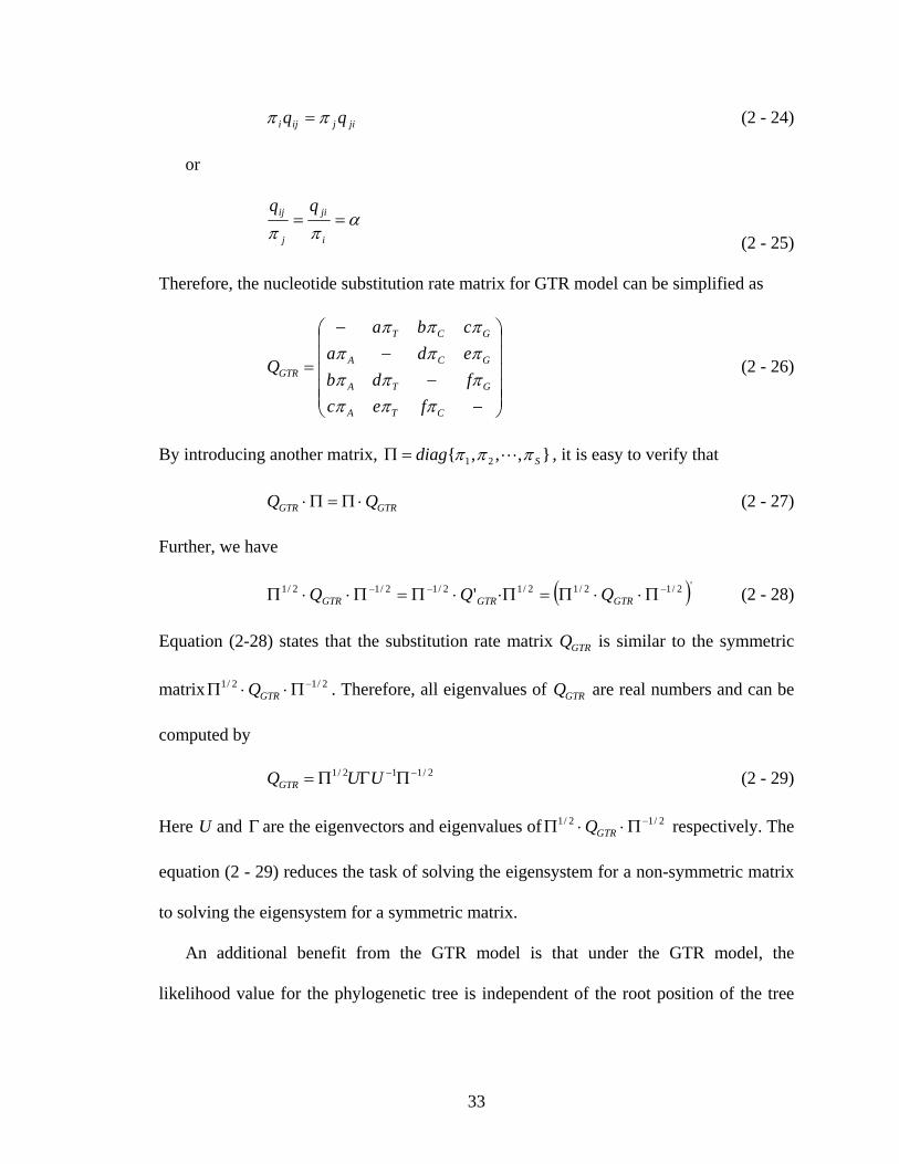
33
jijiji qq ππ = (2 - 24)
or
α
ππ==
i
ji
j
ij qq
(2 - 25)
Therefore, the nucleotide substitution rate matrix for GTR model can be simplified as
⎟⎟⎟⎟⎟
⎠
⎞
⎜⎜⎜⎜⎜
⎝
⎛
−−
−−
=
CTA
GTA
GCA
GCT
GTR
fecfdbedacba
Q
ππππππππππππ
(2 - 26)
By introducing another matrix, },,,{ 21 Sdiag πππ=Π , it is easy to verify that
GTRGTR QQ ⋅Π=Π⋅ (2 - 27)
Further, we have
( )'2/12/12/12/12/12/1 ' −−− Π⋅⋅Π=Π⋅⋅Π=Π⋅⋅Π GTRGTRGTR QQQ (2 - 28)
Equation (2-28) states that the substitution rate matrix GTRQ is similar to the symmetric
matrix 2/12/1 −Π⋅⋅Π GTRQ . Therefore, all eigenvalues of GTRQ are real numbers and can be
computed by
2/112/1 −− ΠΓΠ= UUQGTR (2 - 29)
Here U and Γ are the eigenvectors and eigenvalues of 2/12/1 −Π⋅⋅Π GTRQ respectively. The
equation (2 - 29) reduces the task of solving the eigensystem for a non-symmetric matrix
to solving the eigensystem for a symmetric matrix.
An additional benefit from the GTR model is that under the GTR model, the
likelihood value for the phylogenetic tree is independent of the root position of the tree
34
[114]. Therefore, we can the change the root position at free without changing the
likelihood value of the tree.
2.5.4 Rate heterogeneity among different sites
In the previous discussion, the molecular substitution models are derived based on a
single homologous site. Because the mutation events are constrained by physical and
chemical structures of the DNA and protein molecular, and purified by natural selection,
substitution rate varies greatly among different genes, different codon positions, and
different gene regions [17]. Rate heterogeneity among different sites is accommodated by
including an additional related rate coefficient r in the substitution rate matrix, i.e.
( ) rQtP t e= (2 - 30)
There are several possible ways to determine r [77]:
(1) Assigning different r and different substitution rate matrix to different partitions of
the dataset (by genes or by positions in the codon) [77];
(2) Assuming r at each site is drawn independently from a distribution, such
distribution could be continuous (such as Gamma distribution [119-121] or Log
distribution) or discrete (assume several categories of rate and each has a separate
probability to be chosen);
(3) Assume some fraction of the sites is invariable (i.e. 0=r ) while others mutate at
constant rate [77];
(4) Combining several methods, for example, “invariant + gamma” model.

35
2.5.5 Other more realistic evolutionary models
Considerable amount of effort has targeted in developing more realistic evolutionary
model. Felsenstein and Churchill proposed Hidden Markov model (HMM) to
accommodate rate variance [122] along the sequences. Similarly, the assumption that rate
should be the same in all branches of the trees also needs to be relaxed and a variety of
methods have been proposed.
The gaps within the alignments provide important phylogenetic signals. However
they are often neglected or removed in common phylogenetic inference
methods/packages. Some models have been proposed to incorporate gap in evolutionary
models for phylogenetic inference. These developments include the fragment substitution
model proposed by Thorne et al. [123], the tree HMM approach by Mitchison & Durbin
[23, 123, 124]. In the future, incorporation of rate variation correlated with the three
dimensional structure may be needed [21].
2.6 Likelihood function and its evaluation
Evaluating the likelihood of the data under a given model is a key component in Bayesian
phylogenetic inference and maximum likelihood estimation. Most computation time in
likelihood-based phylogenetic inference methods is spent in likelihood evaluation.
2.6.1 The likelihood function
The likelihood of a specific phylogenetic modelΨ is proportional to the probability of
observing the dataset }{ ijxX = given the phylogenetic model Ψ . Here we assume N is
the number of taxa and M is the sequence length. Each site ),,,( 21 Muuuu xxxx = is an

36
individual observation. The probability of observing the nucleotide pattern at site depends
on the phylogenetic model Ψ , which includes a phylogenetic tree T , a vector of branch
length ( )3221 ,,, −= Nττττ , and an evolutionary model θ .
As described in the previous section, the model of molecular evolution gives the
probability of a mutation from the thi − state to the thj − state at a site u over a finite
period of time t . This transition probability is computed as
( )θ,,|)( tisjsptpij === , (2 - 31)
Here i is the starting state, j is the ending state, and t is the divergence time (i.e. the
length of the branch). )(tPij is computed by equation (2-13) when the substitution rate
matrix }{ ijqQ = is known. The substitution rate matrix is determined by θ , parameters
of an evolutionary model.
The probability of observing the data at a site u given the phylogenetic tree is a sum
over all possible states at the internal nodes of the tree, which is computed by
)),,|(),,|((),,|(1221
12
,
22
1 1
)()(∑ ∏ ∏−++
−
−
+= =
×=NNN
N
aaa
N
Ni
N
ii
iu
iui
iu
iuau axpaapTxL θτθτπθτ αα (2 - 32)
In the above equation, )(iα denotes the immediate ancestral node of node i , iua denotes
the residual state at node i , and iux denotes the residual at the u th site of the i th
sequence.
When rate heterogeneity across different sites is considered, and we assumes the rate
at a site follows a distribution )|( αrf with the shape parameterα (e.g., the gamma
distribution), equation (2 - 32) is replaced by

37
∫ ∑ ∏ ∏∞ −
+= =⎟⎟⎠
⎞⎜⎜⎝
⎛⎟⎟⎠
⎞⎜⎜⎝
⎛×=
+++
−0
,
22
1 1
)()( )|(),,|(),,|(
),,,|(
122112 drrfaxpaap
TxL
NNNN
aaa
N
Ni
N
ii
iu
iui
iu
iua
u
αθτθτπ
αθτ
αα (2 - 33)
Equation (2 - 33) can be approximated by replacing the continuous gamma distribution
with a discrete gamma distribution [125].
Assuming the observation at each site is independent, the likelihood to observe the
entire sequence is:
∏=
=M
uu TxLTXL
1
),,|(),,|( θτθτ (2 - 34)
Generally, a logarithmic form of the likelihood is used because the likelihood itself is
very small number.
2.6.2 Felsenstein’s algorithm for likelihood evaluation
The probability given by (2 - 32) and (2 - 34) can be computed by traversing the tree in
post order using the algorithm proposed by Felsenstein [114]. Let ( )aLp ku
| denote the
probability of all the leaves below node k when the state at site u on node k is a and uL
denotes the likelihood of all leaves at site u .
The Felsenstein algorithm is shown in Figure 2-6. Starting from the leaves, the
Felsenstein’s algorithm continuously prunes the subtrees through step 9-14 until there are
no other nodes left except the root.
Without redundant computation, the Felsenstein’s algorithm needs about
(2 1)NMS S + multiplication operations in step 4. The memory space requirements vary
with implementation. If the site likelihood values at the most recently visited nodes are
saved, only 216 24NS MS NM+ + byte memory space is needed: the first item stores the

38
transition matrix for each branch (there are total 2 2N − branches for a rooted tree); the
second item stores the site likelihood of current node and its two children; and the third
item stores the data matrix. However, this scheme will cause the algorithm to re-compute
the site likelihood for all nodes even if only a small portion of the tree has been changed
between two adjacent likelihood evaluations.
Computer-Node-Likelihood ( k ) 1. Compute-Transition-Matrix ( )(kP , kτ ) 2. If Leaf-Node ( k ) 3. Then 4. For 1←u ; Mu ≤ ; 1+← uu
5. If kuxa =
6. Then 1)|( ←aLp ku
7. Else 0)|( ←aLp ku
8. Else 9. i←k.leftChild; j←k.rightChild
10. Compute-Transition-Matrix ( ( )iP , iτ ) 11. Compute-Transition-Matrix ( ( )jP , jτ )
12. For 1←u ; Mu ≤ ; 1+← uu 13. Foreach StatesofSeta −−∈
14. ( | ) ( | ) ( | , ) ( | ) ( | , )k i ju u i u i
b c
p L a p L b p b a p L c p c aτ τ⎛ ⎞ ⎛ ⎞← ⋅ ⋅ ⋅⎜ ⎟ ⎜ ⎟
⎝ ⎠ ⎝ ⎠∑ ∑
Computer-Tree-Likelihood ( T ) 15. 0ln ←L 16. Computer-Node-Likelihood ( 2N-1 ) 17. 0←uL
18. For 1←u ; Mu ≤ ; 1+← uu
19. 2 1( | )Nu a u
aL P L aπ −←∑
20. )ln(lnln uLLL +=
Figure 2 - 6: The Felsenstein algorithm for likelihood evaluation

39
2.7 Optimizations of likelihood computation
The likelihood evaluation can be optimized in several ways between two adjacent
evaluations of tree likelihood.
2.7.1 Sequence packing
Repeated patterns are common for real datasets used in phylogenetic inference. The
length of the sequences can be cut down by packing the sites with the same pattern and
speed up the likelihood computation. For example, if there are w columns of all state “a”
in the dataset calculate the likelihood of this once and raise it to the power of w. Through
sequence packing, equation (2 - 34) is replaced by
∏=
=P
uppp TxLwTXL
1
),,|(),,|( θτθτ (2 - 35)
Here P is the total number of site patterns, pw is the weight of pattern (i.e. the number of
sites with pattern p ), and ( )θτ ,,| TxL pp is the site likelihood of pattern.
Sequence packing can reduce the likelihood computation by MP
−1 . Here P is the
number of unique site patterns; M is the number of characters.
2.7.2 Likelihood local update
Since in most MCMC algorithms the phylogenetic model changes continuously and
the change between two adjacent generations is small, if we record nodes affected by a
change in the parameter values and trace them back to the root, then only the conditional
probability of those nodes appearing in the back tracing path needs to be recomputed; all
other parts of the computation remain the same. We call this shortcut a local update of the

40
likelihood. Figure 2-7 shows how local update works. The local update can reduce the
average number of nodes to be evaluated from N to Nlog21 . The disadvantage is that all
the conditional probability values in the previous computation need to be kept in the
memory, increasing the memory requirement to 216 8NS NMS NM+ + : the first item
stores the transition matrix for each branch; the second item stores the likelihood for all
internal nodes; and the third item stores the data matrix (we time a multiplier of 8 for
likelihood and transition probability since they are stored as double precision numbers).
When N is large, the local update schema can speed up the likelihood evaluation
remarkably. For this reason, most Bayesian inference programs adopt local update
schema despite the additional memory requirement. However, smart memory
management is required to keep the local update property without frequent data copy
operations.
rootc
ab
If branch a-b has been changed, only the nodes in the path from node a to the root need to recomputed to get the likelihood of the tree.
Figure 2 - 7: Illustration of likelihood local update

41
2.7.3 Tree balance
After multiple mutation operations, the current tree may become imbalanced: one subtree
of the root is much deeper than the other subtree. We define the depth of a subtree as the
maximum number of internal nodes from the root of this subtree to any leaf nodes in the
subtree. As discussed above, the average number of nodes to be re-computed for local
update is 1 log( . )2
root depth ; reducing the depth of the root can speed up the computation
because there are fewer nodes to be recomputed. The tree balancing algorithm is shown
in Figure 2-8.
2.8 Markov Chain Monte Carlo methods
2.8.1 The Metropolis-Hasting algorithm
Though Bayesian analysis of phylogeny provides a direct, formal approach of dealing
with uncertainty in phylogenetic inference with sophisticated statistical models, the
computations required by integrations over unknown parameters is a major obstacle.
tree-balance ( T ) 1. root← T .root 2. gap←depth(root.leftChild) – depth(root.rightChild) 3. If abs(gap) < 2 4. Then return 5. Else node←root 6. For i←0; i≤ abs(gap)/2; i← i+1 7. If depth(node.leftChild)> depth(node.rightChild) 8. Then node←node.leftChild 9. Else node←node.rightChild 10. Tree-Reroot ( T , node )
Figure 2 - 8: The tree-balance algorithm

42
Until the advancement of computing technologies and the introduction of Markov Chain
Monte Carlo methods, Bayesian phylogenetic inferences weren’t feasible.
Markov Chain Monte Carlo refers to a class of methods that simulate random
variables from a target distribution, known up to a normalizing constant. The basic idea
of the MCMC methods is first to construct a Markov chain that has the space of the
parameters to be estimated as its state space and the posterior probability distribution of
the parameters as its stationary distribution. Next, simulate the chain and treat the
realization as a hopefully large and representative sample from the posterior probability
of the parameters of interests. Two major strategies can be used to construct the Markov
chains for exploring posterior distribution: the Metropolis-Hasting algorithm [126, 127]
and the Gibbs sampler [128].
When applied to phylogenetic inference, the Metropolis-Hasting algorithm can be
descried as follows (Figure 2- 9):
Metropolis-Hasting algorithm 1. 0=t ; 0
)0( Ψ←Ψ 2. Repeat 3-9 3. Draw a sampleΨ from ( ))(| tq Ψ• 4. Draw a random variable u from a uniform
distribution )1,0(U
5. Compute ( )ΨΨ ,)(tα
6. If ),( )( ΨΨ≤ tu α
7. Then Ψ←Ψ + )1(t
8. Else )()1( tt Ψ←Ψ + 9. 1+← tt .
Figure 2 - 9: Metropolis-Hasting algorithm

43
In the above algorithm, ( )ΨΨ ,)(tα is called the acceptance probability, and its
definition distinguishes different MCMC algorithms. In the original Metropolis algorithm
[126], the acceptance probability is:
( )( )⎟⎟⎠
⎞⎜⎜⎝
⎛ΨΨ
=ΨΨX
Xt
t
||,1min),( )(
)(
ππα (2 - 36)
Hasting [127] extended the original Metropolis algorithm by allowing an asymmetric
proposal probability )|( )(tq ΨΨ and introduced a new transitional kernel
( )( )
( )( )
( )( )
( ) ( )
||( , ) min 1,
| |
tt
t t
qXX q
πα
π
⎛ ⎞Ψ ΨΨ⎜ ⎟Ψ Ψ = ⋅⎜ ⎟Ψ Ψ Ψ⎝ ⎠
. (2 - 37)
The proposal probability (2 - 37) can be in any form that satisfies 0)|( >⋅ Mq . The
choice of )|( Mq ⋅ may affect the convergence rate of the Markov chain.
In (2 - 36) and (2 - 37), ( )X|Ψπ is the posterior distribution of phylogenetic models
which is proportional to the product of the likelihood and the prior probability. As shown
in the form of the acceptance probability, only the likelihood ratio and the prior ratio for
current sample ( )tΨ and candidate sampleΨ are needed to decide whether accepting the
proposal or not; the computation of the normalizing constant in (2 - 2) is unnecessary.
2.8.2 Exploring the posterior distribution
The direct objective of MCMC in Bayesian analysis is to calculate the integral appearing
in the marginal distribution shown in equation (2 - 5) or (2 - 6). Thus an MCMC method
plays the same role as the Monte Carlo integral approximation method. According to the
law of large numbers, the variance of the Monte Carlo integral approximation is
proportional to 1N
, regardless of the dimensionality of the state space of target

44
distribution [129]. Note that N is the number of samples and the variance decrease as N
increases. To directly draw samples from a complex space with high dimensions is
difficult. Metropolis-based MCMC provides an effective method of sampling mechanism
by evolving a Markov chain.
In theory, a Markov chain constructed with the Metropolis-Hasting algorithm will
converge to a stationary distribution if the chain is irreducible, aperiodic, and possesses a
stationary distribution given the chain runs long enough [130, 131]. The irreducible
property requires the chain has a positive probability to move from one state into any
other state in a finite number of time steps, i.e.
( )( )| ( ) 0j iP t s tΨ + = Ψ Ψ = Ψ > (2 - 38)
Here iΨ and jΨ are any pair of states in the state space, t is the current time, s is the
number of time steps needed to move from iΨ to jΨ .
If the chain is irreducible, then the chain can reach any state after a sufficiently large
number of time steps no matter what the starting state is. It is intuitive that all tree
proposal methods shown in Chapter 3 guarantee the irreducible property of the MCMC
chain. Thus MCMC is a promising method for phylogenetic inference.
2.8.3 The issues
Equation (2- 38) does not provide any information regarding how large s must be. As the
length of any MCMC chain used in real analysis is limited, there are risks that some
states are never reached after the chain has been terminated. One fundamental reason is
that the samples generated using Metropolis-Hasting algorithms are dependent samples.
As a result, samples between two time steps are correlated. The samples drawn using

45
MCMC tend to stick around a local optima mode of the target distribution. Due to such
“stickiness”, the chain may mix extremely slowly: it may take a huge large number of
time (perhaps infinite) steps for the chain to move from one mode to another mode.
Increasing the mixing rate of an MCMC chain may improve the quality of the
posterior distribution approximated by the chain. However, if the chain moves too fast,
the acceptance ratio (the ratio of the number of accepted proposals to the total number of
proposals) become very low and a large percentage of computation is wasted; if the chain
moves too slowly, the acceptance ratio is high but it may take a extraordinary large
number of time steps for the chain to converge [132]. Neither is satisfactory.
The quality of the posterior distribution sampled by a MCMC sampler is critical to
the accuracy of the conclusions summarized from the distribution. If the approximated
distribution ( )π Ψ deviates from the real distribution, ( )π Ψ , the conclusions based on
( )π Ψ may be completely misleading. For example, a poorly implemented Markov chain
may be trapped at local optima localΨ , thus samples generated from this chain give an
extremely high posterior probability for localΨ which is far away from the truth.
Therefore, some practical issues exist for the original Metropolis-Hasting and have to
be avoided in implementation.
1) Choosing the appropriate proposal steps;
2) Making the chain move fast when exploring a posterior distribution in a high
dimensional parameter space;
3) Avoiding the chain stop at local optima; and
4) Detecting the halting time for the chain.

46
2.9 Summary of the posterior distribution
Once the posterior probability has been approximated with MCMC samplers, various
kinds of information can be summarized from such posterior distribution.
2.9.1 Summary of the phylogenetic trees
The posterior probability of phylogenetic trees can be summarized in several ways:
I. Summarizing with the posterior probability of trees. The occurring frequency of a
phylogeny in the samples can be interpreted as an approximation of its posterior
probability. By ranking the trees in the order of their posterior probability, the 99%
credible set of trees can be obtained. Among these trees, the one with the maximum
posterior probability is called the MPP tree.
II. Summarizing with the posterior probability of clades. A clade is the group of taxa
which is included in the same partition divided by an internal branch. Similar to the
posterior probability of the phylogenetic tree, the frequency of a clade in the
samples can be interpreted as its posterior probability. Using the clade posterior
probability distribution and a specific consensus rule, a consensus tree can be
constructed as the summary of the posterior probability of the clades.
III. Summarizing with the likelihood values. Though seldom used in practice, the
samples can also be summarized using their likelihood values as maximum
likelihood methods.
2.9.2 Summary of the model parameters
When model parameters are also included as the interested of state parameters in MCMC,
Bayesian analysis also output samples drawn during the MCMC run. Model parameters

47
and some evolutionary characteristics (e.g. tree length, distance between two partitions
separated by an internal branch) can be summarized from the approximated posterior
distribution samples from Bayesian phylogenetic inference using conventional statistical
methods.
2.10 Chapter summary
This chapter provides an overview of phylogenetic inference method and the framework
of Bayesian phylogenetic inference. There are various competing phylogenetic methods
to build a phylogenetic tree from a dataset which provides clues for the evolutionary
history of a set of taxa. These methods may use different source of data, different
optimality to choosing the closest estimation. But their common objective is same:
estimating the correct tree, or if impossible, making the estimation close to the true tree
as much as possible.
When the phylogenetic trees become large and large (up to thousands and ten of
thousands of taxa), advanced algorithms and high performance implementations become
critical to guarantee the estimated trees close to the true tree sufficiently. In this
dissertation, we choose Bayesian methods as a possible candidate to infer large
phylogenies.
Bayesian phylogenetics inference is founded on likelihood function for a dataset
under some phylogenetic model. It is a twin of Maximum Likelihood Estimation, both
require explicit probabilistic model of evolutions.

48
The computational complexity of Bayesian phylogenetic inference is handled by a
family of Markov Chain Monte Carlo methods which can be viewed as a sampling
method or a stochastic search method depending on the interest of study and context.
Using MCMC, both the posterior distributions of phylogenetic trees and the
parameters in the model of evolution can be approximated and conventional statistic
procedure can be applied to summarize the variables of interest.

49
Chapter 3
Improved Monte Carlo Strategies
3.1 Introduction
As described in Chapter 2, Bayesian phylogenetic inference relies on the posterior
distribution approximated by Markov Chain Monte Carlo (MCMC) methods. The quality
of the posterior distribution sampled by a MCMC sampler is critical to the accuracy of
the conclusions. If the approximated distribution deviates from the real distribution, the
conclusions may be completely misleading, as observed in the literature [49, 50].
Though the MCMC method plays a critical role in Bayesian phylogenetic inference,
there are few studies of its performance due to its computational expense. Developing
better MCMC strategies and studying their performance are necessary for two reasons:
1) Some experimental results indicate that Bayesian phylogenetic inference using
MCMC (BMCMC) produces misleading posterior probability for trees and clades
under some evolutionary scenarios. It is not clear whether the MCMC implementation
or some deeper reasons in the Bayesian phylogenetic inference is responsible for such
discrepancies.

50
2) There is no theoretical or formal proof to detect or guarantee that an MCMC run will
converge to the correct posterior distribution after the chain stop at a certain number
of time steps.
Thus, improved MCMC strategies are required for more robust, more efficient
Bayesian phylogenetic inference. This chapter provides our observations and
improvements for MCMC strategies for use in Bayesian phylogenetic inference.
3.2 Observations
To illustrate the problem in MCMC implementation, we use the Metropolis-Hasting
algorithm to approximate the distribution shown in Figure 3-1. The target distribution has
the analytical form
( )212
32
1[0,1]( )
0 [0,1]
i
x
ii
c a e xf x
x
μσ−
−
=
⎧⎪ ∈= ⎨⎪
∉⎩
∑ (3 - 1)
A Distribution with Three Modes
0.0
1.0
2.0
3.0
4.0
5.0
0.0 0.1 0.2 0.3 0.4 0.5 0.6 0.7 0.8 0.9 1.0
x
p.d.
f
Figure 3 - 1: A target distribution with three modes

51
where 1 0.5a = , 1 0.1μ = , 1 0.04σ = , 2 1.0a = , 2 0.5μ = , 2 0.04σ = , 3 0.5a = , 3 0.9μ = ,
3 0.04σ = and 5.0c = . The modes of this target distribution are 0.1 , 0.5 and 0.9 .
We use the delta method described in the previous section to propose a candidate
sample point which uses Equation (3-2) to draw a new proposal point, namely:
( ) ( ) ( )1 0.5x t x t uλ+ = + ⋅ − , (3 - 2)
Approximated Distribution Using Metropolis Algorithm (lamda=0.7, x0=0.5)
0.01.02.03.04.05.06.0
0.0 0.1 0.2 0.3 0.4 0.5 0.6 0.7 0.8 0.9 1.0
x
p.d.
f
(a)
Approximated Distribution Using Metropolis Algorithm (lamda=0.2, x0=0.5)
0.02.04.06.08.0
10.012.0
0.0 0.1 0.2 0.3 0.4 0.5 0.6 0.7 0.8 0.9 1.0
x
p.d.
f
(b)
Figure 3 - 2: Distribution approximated using Metropolis MCMC methods

52
The target distribution seems simple, but it is difficult to approximate accurately
using an MCMC constructed with the original Metropolis-Hasting algorithm. Figure 4-2
shows the two approximations using 0.7λ = and 0.2λ = . Both chains start at ( )0 0.5x = .
Though all three modes appear in the approximation shown in Figure 3-2 (a), the
shape of each mode differs from the target distribution slightly. In Figure 3-2 (b), the
approximation shows only one mode; the other two modes have disappeared. Neither
shows the expected distribution from Figure 3-1.
Samples Drawn at Each Time Step (lamada=0.7, x0=0.5)
0.0
0.2
0.4
0.6
0.8
1.0
0 100 200 300 400 500 600 700 800 900 1000
Time Step (t)
x
(a)
Samples Drawn at Each Time Step (lamada=0.2, x0=0.5)
0.0
0.2
0.4
0.6
0.8
1.0
0 100 200 300 400 500 600 700 800 900 1000
Time Step (t)
x
(b)
Figure 3 - 3: Samples drawn using Metropolis MCMC method

53
Figure 3-3 shows samples drawn at each time step during the above two
approximations. We observe that for larger proposal steps, the chain mixes faster; for a
smaller proposal step, the chain “sticks” around a local mode.
For the above example, though the target distribution is known and simple, it is
nontrivial to choose a proper proposal step parameter to achieve an efficient MCMC
chain. Intuitively, since we know little about the shape of posterior distribution of the
phylogenetic model, we have to be cautious in interpreting the summary of the posterior
distribution sampled using MCMC methods. At the same time, we must develop more
robust MCMC methods and investigate their performance in practical Phylogenetic
inference.
3.3 Strategy #1: reducing stickiness using variable proposal step length
In the previous section, we discussed the risks that a Markov chain constructed using the
Metropolis-Hasting algorithm may be trapped by a local mode and fail to explore the
desired distribution. Changing proposal step length may improve the mixing property of
an underlying Markov chain.
According to the irreducible property requirement, to approximate the target
distribution correctly, at time t , the chain must have a positive probability to move from
one state iΨ into any other state jΨ in a finite number of time steps s , i.e.
( )( )| ( ) 0j iP t s tΨ + = Ψ Ψ = Ψ > . (3 - 3)
Under ideal situations, the chain can move from one state to any other state within
one step (as shown in Figure 3-4). According to a proof of the MCMC algorithm [130],

54
the chain will approximate the distribution accurately. However, such a situation is rare;
the chain actually needs to traverse some intermediate states to reach another state. If the
transition probability between the intermediate states are smaller than some threshold, the
probability given in (3 – 3) may be close to 0, which means the target state will never be
reached and the theoretical approximation has a large deviation from the real
approximation.
Therefore, we proposed a variable step length MCMC which draws the step length
from certain distributions (for example, a uniform distribution); we used this step length
to propose a new candidate state. Using variable step length, we can move the chain
between different states more freely and overcome its “stickiness” to local optimal mode.
Figure 3-5 shows the approximation of the target distribution shown in Figure 3-1.
The distribution of the samples is close to the target distribution, both in the number of
modes and in the shape of each mode.
The number of possible states of phylogenetic trees, even for a small number of taxa,
is extraordinary large. However, the distance between any two states is less than the
number of taxa, even using the simplest tree proposal method, such as NNI (Nearest
Neighbor Interchange). We used the extended tree mutation operator for variable step
length proposal in phylogenetic inference; this algorithm is shown in Sections 3.6.
Figure 3 - 4: Illustration of state moves

55
3.4 Strategy #2: reducing sampling intervals using multipoint MCMC
Choosing a good proposal mechanism is very difficult in phylogenetic inference.
Variable step length MCMC can reduce the risk of trapping local optima. But it
introduces another issue: low acceptance rate. A chain must try many proposals to accept
one successful candidate, which usually requires a large sampling interval.
One strategy is to propose multiple sample candidates and consider their combined
effects in deciding the next move of the Markov chain. We call this strategy multipoint
MCMC. In this dissertation, we implemented a variant of multipoint MCMC proposed by
Liu et al. [132]. Figure 3-6 illustrates the process of multipoint MCMC. This algorithm
includes 4 steps:
1) Propose K samples 1 2, , , KX X X from the distribution of X ;
2) Select a candidate Y from 1 2, , , KX X X according to the probabilities of
1 2, , , KX X X ;
Approximated Distribution Using Metropolis Algorithm (lamda=variable, x0=0.5)
0.01.02.03.04.05.06.0
0.0 0.1 0.2 0.3 0.4 0.5 0.6 0.7 0.8 0.9 1.0
x
p.d.
f
Figure 3 - 5: Approximated distribution using variable step length MCMC

56
3) Propose K samples 1 2, , , KY Y Y from the distribution of Y ;
4) Accept Y with acceptance ratio
( ) ( ) ( )( ) ( ) ( )1 2
1 2
, , ,min 1,
, , ,K
K
w X X w X X w X Xr
w Y Y w Y Y w Y Y⎛ ⎞+ +
= ⎜ ⎟⎜ ⎟+ +⎝ ⎠. (3 - 4)
and reject it with 1 r− .
In equation (3 – 4), ( )( , ) ( , ) ( , )w X Y X T X Y X Yπ λ= , ( , )T X Y is an arbitrary
proposal function, and ( , )X Yλ is an arbitrary, symmetric, non-negative function.
In our implementation, we chose
( )( ) ( ) ( )*
*( , ) ln lni
i i
Xw X X L X L X
Xππ
= = − (3 - 5)
and
( )( ) ( ) ( )*
*( , ) ln lni
i i
Yw Y Y L Y L X
Xππ
= = − . (3 - 6)
Figure 3 - 6: The multipoint MCMC
57
Thus, the acceptance ratio r becomes:
1 2
1 2
ln ( ) ln ( ) ln ( )ln ( ) ln ( ) ln ( )
K
K
L X L X L XrL Y L Y L Y
+ + +=
+ + + (3 - 7
We can use a similar technique [132] to prove that the above algorithm will correctly
approximate the posterior distribution of phylogenetic models.
Though multipoint MCMC allows the chain to keep moving with a large step size,
one potential issue is that if the step length is still small and the distribution has multiple
modes, multipoint MCMC may fail just as often as the classical Metropolis algorithms.
By combing multipoint-MCMC with variable step length to draw candidate samples with
different step sizes, we can overcome this issue.
3.5 Strategy #3: improving mixing rate with parallel tempering
As shown in Section 3-2, a target distribution may contain multiple modes which are
separated by high energy barriers, or low probability regions. In phylogenetic inference,
such regions could be phylogenetic models with low likelihood scores. If a proposal
mechanism fails to draw candidate samples in regions which are separated from current
states by low probability regions, the chain may seem to converge, but the approximation
is far from complete.
One strategy is to use an augmented distribution { }( )i xπΠ = )..1( mi = , which
consists of multiple “tempered” distributions, each distribution having a different
temperature iT . Increasing iT will result in a flatter distribution, given a heating schema
like

58
( ) ( )1 10
iTiπ π += . (3 - 8)
Figure 3-7 shows four tempered distributions based on the target distribution given in
Figure 3-1. The temperatures of the four distributions are 0.0, 1.0, 3.0, and 8.0.
Intuitively, Metropolis algorithms can approximate a flatter distribution accurately. This
was verified in our simulation.
Figure 3 - 7: A family of tempered distributions with different temperatures
The Metropolis-coupled MCMC, first proposed by Geyer [133, 134] was also called
Parallel Tempering, exchange Monte Carlo, or (MC)3. This strategy currently has been
adopted in MrBayes [58]. The idea of Metropolis-coupled MCMC is to run several chains
in parallel, each chain having a different stationary distribution )(Ψiπ , and with index
swap operations conducted in place of the temperature transition of simulated annealing.
The chain with distribution )(1 Ψπ is used in sampling and is called the cool chain. The
other chains are used to improve the mixing of the chains and are called heated chains.
The Metropolis-coupled MCMC algorithm is shown in Figure 3-8.
A family of tempered distributions
0.0
1.0
2.0
3.0
4.0
5.0
0.0 0.1 0.2 0.3 0.4 0.5 0.6 0.7 0.8 0.9 1.0
x
p. d
. f.
T=0.0T=1.0T=3.0T=8.0

59
An alternative is to combine the parallel step and the swap step into a super step and
conducts a swap step at every generation. A parallel version of Metropolis-coupled
MCMC was implemented in this dissertation and will be described in Chapter 4.
There are three related questions when applying Metropolis-coupled MCMC in
Bayesian phylogenetic inference:
1) How many chains are needed?
2) Which heating schema should be used?
3) Will Metropolis-coupled MCMC fail?
How many chains to use is an empirical issue. Usually, more chains will provide
more chances to improve the mixing rate and avoid local optima, but more chains also
incur a higher computational cost. Parallel computing can keep the total time from
Metropolis-coupled MCMC 1. 0t ← ; 2. For 1i ← to m
3. ( ) 0ti iΨ ←Ψ
4. While (stop-condition-not-met) 5. Draw random variable 1u from )1,0(U
6. If 1 0u α≤ 7. Then do-classical-MCMC in parallel 8. Else //do a chain swap operation 9. choose two chains i and j
10. compute ( ) ( )
( ) ( )
( ) ( )min 1,
( ) ( )
t ti j j i
s t ti i j j
aπ ππ π
⎧ ⎫Ψ Ψ⎪ ⎪= ⎨ ⎬Ψ Ψ⎪ ⎪⎩ ⎭
11. Draw random variable 2u from )1,0(U
12. If 2 su α≤
13. Then swap-index-temperature ( ),i j
14. 1t t← +
Figure 3 - 8: The Metropolis-coupled MCMC algorithm

60
increasing as the number of chains increase. We observed the benefit of choosing the
number of chains according to the heating schema and the target distribution.
Assuming two adjacent chains with temperature iT and 1iT + , there is a rough
relationship among chain temperatures, the logarithm format likelihood, and the desired
acceptance ratio,
( ) ( )( ) ( )
1
1
1 11 1
11 1
1 11
i i
i i
T Ti i
T Ti i
π πα
π π
+
+
+ ++
+ ++
≈ . (3 - 9)
From (3 – 9), we have
1
1 1 ln log1 1i i
LT T
α+
⎛ ⎞− Δ ≈ −⎜ ⎟+ +⎝ ⎠
. (3 - 10)
Here, ln LΔ is the typical difference of the logarithmic form of the likelihood which can
be obtained by averaging the differences between random samples and the one estimated
using maximum likelihood; α is the lower bound of the acceptance ratio of the chains.
During our experiments, we observed that for phylogenetic inference problems with a
large number of taxa, Metropolis-coupled MCMC may have very low acceptance ratios.
3.6 Proposal algorithms for phylogenetic models
A phylogenetic model ( ), ,T τ θΨ = Ψ includes three components: a tree topology (T ); a
vector of branch lengths ( 1( , , )nτ τ τ= , where n is the number of branches); and the
parameters of an evolutionary model ( ( )1, , mθ θ θ= , where m is the number of the
parameters for describing the model). Thus, a phylogenetic model is in the
space T τ θΩ = × × , which consists of discrete sub-spaces separated by all possible tree
topologies. Another characteristic of this space is that m varies with different model

61
assumptions (for example, 1m = for the JC69 model; 6m = for the HKY model; and
10m = for the GTR model).
An MCMC method is essentially a sampler which draws dependent samples from the
target distribution using one or more Markov chains constructed using Metropolis-
Hasting algorithms or their variants. We break an MCMC sampler into two parts: 1)
generate a proposal for the next move, and 2) design a transition function to guide the
move. In this section, we discuss how to generate a proposal in the space of phylogenetic
models, i.e. T τ θΩ = × × .
There is one discrete random variable, T , and there are n m+ continuous random
variables 1 1, , , , ,n mτ τ θ θ for one state in the phylogenetic model spaceΩ . The Gibbs
sampling strategies provide various mechanisms to update each component either
randomly or systematically [132]. The random-scan Gibbs sampler chooses a component
c at random and then draws a sample from ( )( )tcπ −⋅ Ψ and leaves other components
unchanged at time step t . A system-scan Gibbs sampler updates every component in
order within one super step. Therefore, given the current phylogenetic model state ( )tΨ ,
we can propose a new state by updating T , iτ and iθ separately.
3.6.1 Basic tree mutation operators
A new tree topology can be generated by mutating current topology through three basic
tree operators: NNI (Nearest Neighbor Interchanges), SPR (Subtree Pruning-Regrafting),
and TBR (Tree Bisection-Reconnection) [77].
1) NNI changes a tree topology locally. Any internal branch ( ),b u v= of a tree
topology connects four subtrees ( A , B , C , and D ), where u and v are the

62
labels of the two nodes connected by b . Assuming the original tree topology is
( ), | ,A B C D , two additional tree topologies ( ), | ,A C B D and ( ), | ,A D B C are
obtained by swapping one subtree of node u and one subtree of node v .
3) SPR prunes a subtree sT from the current tree T and then attaches sT to a branch of
the pruned tree \ sT T . Assuming the number of leaves in T is n and the number of
leaves in sT is m , then 2( ) 3n m− − topologies may be obtained from a single SPR
operation.
4) TBR partitions a tree T into two subtrees ( AT and BT ) along a branch, chooses one
branch a from AT and another branch b from BT . Then a new topology can be
obtained by connecting branch a and branch b . Assuming the number of leaves on
AT is an and the number of leaves on BT is bn , a single TBR operation can result in
( )( )2 3 2 3a bn n− − new topologies.
It can be shown that NNI, SPR, and TBR can change any tree topology into any other
tree topology with a finite number of mutation operations used separately. This is true
under the condition that all proposed moves will be accepted; it may be not true if the
move is subjected to selection according to its likelihood score because a high energy
barrier (or low probability region) will constrain the move around some local optima.
3.6.2 Basic tree branch length proposal methods
The length of a branch can be any real number within the interval ( )0,∞ . Two proposal
methods can be used to propose new branch lengths: the scaling and delta methods.

63
3.6.2.1 The scaling method
Denote the current branch length 0τ . A new branch length is generated as ( 0.5)0
ueλτ τ −= ,
where u is draw from a uniform distribution (0,1)U . When 0.5u < , the branch is
shortened; when 0.5u > , the branch length is extended. The parameter λ controls the
range of the proposed branch length.
3.6.2.2 The delta method
The delta method adds a mutation to the current branch length as ( )0 0.5uτ τ λ= + − ,
where u is draw from a uniform distribution (0,1)U , and λ controls the step length.
3.6.3 Propose new parameters
Basically, the method for proposing branch lengths can be used to propose a new
parameterθ . Some prior distributions can be used to increase the acceptance ratio. For
example, the distribution of the frequencies of all nucleotide states can be drawn from the
Dirichlet distribution.
3.6.4 Co-propose topology and branch length
Tree topology and branch length can be updated simultaneously using a single tree
mutation. Two methods have been proposed in the past: the Traversal profile method
[40]and the LOCAL methods [41].
3.7 Extended proposal algorithms for phylogenetic models
This section presents our extension of the basic proposal algorithm described in previous
sections.

64
3.7.1 Extended tree mutation operator
As discussed in Section 4.3, in order to avoid local optima phenomena in MCMC
sampling, we need to design tree mutation operators that can move rapidly in the tree
space. The idea is to combine multiple basic tree mutations within one operator, which
we name extended tree mutation operators. We use parameter D to control the maximum
number of basic tree mutations in an extended tree mutation operator. An extended tree
mutation operator work as follows:
We can choose a proper distribution ( )f k to control the percentage of NNI, SPR and
TBR. The choice of parameter D depends on the number of leaves of the tree topology.
An extended tree mutation can discover as many as DN topologies, where N is the
number of tree topologies that can be explored by a single basic tree operator.
3.7.2 Multiple-tree-merge operator
Most tree search methods search the optimal tree along a single trajectory. Larger spaces
can be explored using multiple independent trajectories. After some training period under
the likelihood function, each tree on those independent trajectories may contain some
extended-tree-mutation (T , D) 1. draw d from a uniform distribution (1, )U D
2. 0T T←
3. For 1i ← to d 4. draw k from a distribution ( )f k for 1..3k =
5. If 1k = Then iT ← Tree-NNI( 1iT − )
6. If 2k = Then iT ← Tree-SPR( 1iT − )
7. If 3k = Then iT ← Tree-TBR( 1iT − )
8. Return iT 9.
Figure 3 - 9: The extended-tree-mutation method

65
subtrees which are partially optimal. Merging these optimal subtrees can result in a good
proposal for the next move. This is one of the basic ideas of the genetic algorithm. We
introduce this method here as another tree proposal operator. The multiple-tree-merge
operator merges subtrees from several “good” candidates into a new candidate as Figure
3-10:
For 2K = , the Multiple-tree-merge operator becomes the crossover operator used in
GAML [135].
3.7.3 Backbone-slide-and-slide operator
For any two internal nodes u and v on an unrooted tree, there exists a path from node u
to node v . We call this path backbone u v− . Assuming there are a total of n internal
nodes (including node u and node v ) on backbone u v− , then the backbone connects
2n + subtrees labeled from 1 to n in the order they are visited, from node u to node v .
Label the other subtree of node u as subtree 0 , and the other subtree of node v as
multiple-tree-merge ( 1, , KT T ) 1. draw k from a uniform distribution (1, )U K
2. 0 kT T←
3. For 1i ← to K 4. If i k≠ Then 5. Select a subtree sT from iT
6. For each leave node in sT , prune it from 0T ,
denote the pruned tree 0 \ sT T
7. Attach sT to 0 \ sT T at a random branch, replace 0sT with the new tree
8. Return 0T
Figure 3 - 10: The multiple-tree-merge method

66
subtree 1n + . Arrange subtree 0 , subtree 1n + and all internal nodes into one vertical
line, and denote the distance from each internal node to subtree 0 iy . Then we randomly
choose one internal node k , and slide it along the backbone by drawing a random
number y from a uniform distribution 1(0, )nU y + . The value of y will decide the new
position of node k. Finally, we scale the length of the backbone.
The backbone-slide-scale method is shown in Figure 3-11, it is an extension of the
LOCAL method proposed by Larget et al. [41] when the back bone includes two nodes.
3.8 Chapter summary
MCMC is the cornerstone of Bayesian phylogenetic inference. The proper
implementation of MCMC is critical to the correctness of Bayesian phylogenetic
u
v
0
1
2
3
4
5
6
0
y1
y3
y4
y5
y2
y6
a
b
c
u
v
0
1
2
3
4
5
6
0
y1
y3
y4
y5
y2'
y6
a
b
c
u
v
0
1
2
3
4
5
6
0
y1*
y3*
y4*
y5*
y2*
y6*
a
b
c
Step 1: Construct the Backbone Step 2: Slide Subtree 3 Step 3: Scale Backbone length
Figure 3 - 11: The backbone slide and scale method

67
inference. In theory an MCMC chain constructed using the Metropolis-Hasting algorithm
will visit every state after a sufficiently large number of time steps. In practice, many
chains can not efficiently mix between two states separated by low probability regions.
We analyzed the dangers of MCMC to output misleading approximations and proposed
several strategies to overcome those pitfalls. The key idea is to design some transitional
kernel which can move from one state to any other state within limited number of steps
without blocking by probable high energy barriers.
We implemented this idea as improved MCMC strategies and extended proposal
methods. Using variable proposal step length, we can bring two distant states close to
each other. Using multipoint MCMC, we can improve the quality of candidate state and
reduce the sample intervals. Using population-based MCMC, we can expand the search
range of the MCMC algorithm. By introducing the above-described proposal methods
and MCMC strategies the steps needed for the chain jump from one state to any other
state is greatly shortened; therefore, the chain can cross valleys much easier.
These described strategies and proposal methods are implemented in PBPI, our high
performance implementation of Bayesian phylogenetic inference.

68
Chapter 4
Parallel Bayesian Phylogenetic Inference
4.1 The need for parallel Bayesian phylogenetic inference
Large phylogenies deepen our understanding about biological evolution and diversity.
With the rapid accumulation of genomic data through various genome sequencing
projects, constructing large phylogenies across the tree of life is becoming a reality.
Simulation studies indicate that the accuracy of a phylogenetic method can be improved
by adding more taxa and including more characters [136].
Bayesian inference of large phylogeny is a computationally intensive process.
Consider a realistic problem: estimating the phylogeny of 200 aligned amino acid
sequences with 3500 characters using a model that allows five different rates across sites
( 200=N , 5000=M , 20=S , and 5=K ). Assume we use a Metropolis-coupled
MCMC algorithm with 5 chains, each chain lasting 100,000,000 generations, and that we
use a local update schema in the implementation. Then we need at least on the order of
1010 bytes of memory space and at least on the order of 1710 multiplication operations. To
be competitive in analytic quality, more complicated models are desirable; this together

69
with an exponential growth rate in the number of sequenced taxa makes growing
computational demand. Even now these demands exceed the ability of a single-CPU
computer and require a longer computation time than is reasonable, hence the motivation
for parallel implementation of Bayesian phylogenetic inference to reduce computational
time.
4.2 TAPS: a tree-based abstraction of parallel system
A parallel system uses a collection of processing elements that communicate and
cooperate to solve large problems faster [137]. Modern computer systems effectively
exploit various hardware parallelisms to gain raw performance at different levels ranging
from instruction, architecture, vector, processor core, microprocessor chip, SMP node,
cluster, and grid. In the past three decades, we have observed tremendous performance
increases and cost decreases in microprocessors, storage, and networking. Beowulf
clusters with hundreds of nodes are common in major universities and research institutes.
The grid, as a new infrastructure, makes sharing geographically-distributed computing
resources a reality.
Parallel algorithm design and analysis relies on an abstract model of parallel
computation to model the key attributes of physical parallel systems. Existing models
include PRAM (parallel random access machine) [138], BSP (bulk synchronous parallel)
[139], LogP [140], and their variants. None of them can be directly applied to grid
systems or clusters of heterogeneous clusters. Therefore, we use TAPS, a tree-based
abstraction of ubiquitous parallel systems, as the model guiding our design and analysis
of parallel algorithms for Bayesian phylogenetic inference.

70
As shown in Figure 4-1, TAPS represents the parallel systems as a rooted-tree, where
all the physical processors are located on the leaves and clusters of computing resources
are represented as an internal node. The root is the largest organization available to the
user. Each leaf node has its independent processing unit ( P ), memory space ( M ) and
network interface ( N ). The internal node is a virtual organization which includes an
interconnection network and a collection of computing resources which could be a
physical processing unit or a lower level virtual organization. Each edge of the tree
represents a communication link with fixed bandwidth and latency. Each node (labeled k )
on the tree incurs an overhead ( ko ) when communicating with other nodes. Similar to the
LogP and Pnlog model [141], the communication cost between a pair of nodes i and
j is modeled as
jiji OLOC ++=, . (4 - 1)
P/M P/MP/M P/M P/M P/MP/M P/M P/M P/Mi j
Li-jOi Oj
A
C
B
LAC
OA
Figure 4 - 1: An illustration of TAPS

71
Here ∑=k
ki oO , k is the node on the path from node i to r , the root of the smallest
subtree shared by node i and j ; ∑=e
elL , e is the edge on the path from node i to r .
Both O and L are system characteristics and vary with message size.
TAPS provides a hierarchical view of a general parallel system which clusters
heterogeneous, distributed computing resources into one virtual platform for parallel
programs. Communications between processing units within a lower level virtual
organization (e.g. an SMP node) have smaller latency and overhead than communications
between nodes that belong to different lower level virtual organizations (e.g. processing
units on two different SMP nodes or two Beowulf clusters). A real system represented by
TAPS is the departmental grid, which consists of several clusters with different kinds of
computing nodes, several SMP systems, and a cluster of loosely connected Linux/Unix
workstations. TAPS is an MPMD system, using MPI (message passing interface) as its
communication mechanism and NFS as its global storage. In this chapter, we discuss
parallel Bayesian phylogenetic inference algorithms based on a system modeled by TAPS.
4.3 Performance models for parallel algorithms
The performance of a parallel algorithm is described by two metrics: speedup and
scalability. Speedup quantifies the performance improvement for a given workload.
Scalability characterizes how speedup varies with the number of processing units and the
size of workload.
The speedup S of workload W on N processing units using algorithm A is defined
as

72
),()(
),( 0
NWTWT
NWSA
A =. (4 - 2)
Here 0T is the execution time for workload W on a single processing unit using an
optimal sequential algorithm; ),( NWTA is the TTS for workload W on N processing
units using algorithm A , which is defined as the maximum of N individual execution
times on the processing units. Ignoring the communication cost and parallelization
overhead, Kruskal and Weiss [142] have shown that for independent subtasks, ),( NWTA
can be approximated as
NN
WTNWTA log21)(
),(
0
σ+=
. (4 - 3)
Here σ is the standard deviation of workload per process and indicates the load
imbalance.
Not all workload can be executed in parallel. If we assumeα percentage of the
workload has to be executed sequentially, then (4-3) should be modified as
NNN
WTNWTA )log21)(1()(
),(
0
σαα +−+=
. (4 - 4)
Parallel algorithms on realistic systems always incur parallel overhead and
communication latency. We assume parallel overhead is dependent on N and
approximated by Nlogβ . We further assume communication breaks the whole execution
time into K super steps, each super step consisting of one computation phase and one
communication phase. Following the abstraction in the last section, the communication
cost can be approximated as ( ) 'log)( NMLOK + , where M is the message size with

73
byte as the unit, and 'N is the number of processing units involved in the communication
phase.
Thus, considering all the above factors, the speedup can be finally approximated as
( ) ))((logloglog21)1(1),(
' MLONWKN
WNN
NNWS A
+⋅⋅+⋅+−+−+=
βσαα. (4 - 5)
The above formula indicates the difficulties of scaling speedup with a large number of
processors for fixed workload. Figure 4-2 illustrates the differences between real speedup
and ideal speedup, and Amdahl’s law (speedup without communication cost) [143].
In realistic scientific computing, such as Bayesian phylogenetic inference, the
workload is not fixed. According to Gustafson’s law [144], the percentage of sequential
execution of the workload may decrease by increasing problem size, thus an improved
speedup can be achieved.
Ideal speedup
Speedup without Communication Cost
Real speedup
# of processing units
Speedup
N
SA(W,N)
Figure 4 - 2: Speedup under fixed workload

74
In summary, there are two kinds of speedup scalability: strong scalability for fixed
problem size and weak scalability for varying problem size. The former indicates for a
given problem, how fast we can get the solution; the later indicates given a time limit,
how big a problem we can solve. Analyzing the performance of parallel algorithms
should consider both of kinds of speedup scalability.
Equation (4-5) also shows that fixed workload speedup can be improved by: 1)
reducing load imbalances across all processing units; 2) reducing communication
frequency; 3) reducing message size per communication; and 4) reducing the number of
processors involved in communication. These principles have been applied in our
implementations of parallel Bayesian phylogenetic algorithms.
4.4 Concurrencies in Bayesian phylogenetic inference
In Figure 4-3, the procedure of a generic Bayesian phylogenetic inference sketches
multiple levels of concurrency:
1) Multiple independent runs for chain convergence detection (lines 7-17);
2) MCMC chains for better chain mixing (lines 8-17);
3) Multiple data partitions for improved model or combined data (lines 10-13);
4) Multiple rate categories for rate variations across sites (lines 12-13); and
5) Multiple sites across the sequence.
Levels 1-4 are conditional on the setting of the Bayesian analysis. Thus, the parallel
algorithm for Bayesian phylogenetic inference should be flexible and automatically
exploit the available parallelism for current analysis setting.

75
Considering the existence of multiple level concurrencies in a Bayesian analysis and
their tolerance for communication latency, we can map each level to a virtual
organization, represented by TAPS (shown as Figure 4-1). For example, we can run site
likelihood in parallel at the SMP node level and run multiple chains at the cluster level.
4.5 Issues of parallel Bayesian phylogenetic inference
Parallelizing Bayesian phylogenetic inference brings two advantages: speeding up the
computation and providing the memory space needed for a competitive biological
analysis of current data. Since generating the Markov chain accounts for the vast bulk of
the computation, our parallelization will focus on the MCMC algorithm. A single chain
MCMC is essentially a sequential program, since the state at time 1+t is dependent on
the state at time t . Multiple dependent chains may increase the mixing rate of the chains
The procedure of a generic Bayesian analysis 1. Read-Dataset 2. Set-Assumption 3. For run=1 to number-of-run 4. For chain=1 to number-of-chain 5. Set-starting-model 6. For time-step=1 to maximum-time-step 7. For run=1 to number-of-run 8. For chain=1 to num-of-chain 9. Propose-candidate-model 10. For partition=1 to number-of-partition 11. For site=1 to number-of-site 12. For rate=1 to number-of-rate 13. Calculate-Site-Likelihood 14. Compute-Tree-Likelihood 15. Make-Accept/Reject-Decision 16. Update-Chain-State 17. Exchange-State-between-chains 18. Detect-Chain-Convergence 19. Analyze-Samples
Figure 4 - 3: The procedure of a generic Bayesian phylogenetic inference

76
and also increase the parallel granularity of Bayesian computation.
One way to parallelize a Metropolis-Hasting MCMC is to parallelize the likelihood
evaluation. Another is to run multiple chains and sample each one after the burn-in stage.
This method may involve many random starting points, which provide the advantage of
exploring the space through independent initial trajectories; however, it also has the
danger that the burn-in stage may not always be cleared. A single Metropolis-coupled
MCMC run can be parallelized on the chain level, but chain-to-chain communications are
needed frequently. However, just parallelizing on the chain level will not use all the
available resources, especially when memory is the limiting factor. Multiple-try
Metropolis methods are easy to parallelize and may reduce the whole computation by
using a shorter chain to get the same result as a long chain. For illustrative purpose we
focus on Metropolis-coupled MCMC in the next chapter.
An important issue in parallelization of Metropolis-coupled MCMC is balancing the
load. This issue of load balancing comes from the fact that when local update schema is
used, different chains will reevaluate a different number of nodes. More seriously, local
update schema are only available for topology and branch length changes; with
parameters such as global rate matrix changing, the likelihood needs to be evaluated
across the tree, so all nodes need to be reevaluated.
Other issues that must be considered in a parallel algorithm are how to synchronize
the processors, how to reduce the number of communications, and how to reduce the
message length of each communication.

77
4.6 Parallel algorithms for Bayesian phylogenetic inference
This section presents a parallel implementation of MCMC algorithms in Bayesian
phylogenetic inference. The MCMC strategy chosen here is the Metropolis MCMC. As
described in Chapter 3, there are two variants of Metropolis-coupled MCMC: simulated
tempering MCMC and parallel tempering MCMC. Both methods build h companion
chains whose distribution is ( ) ( )1/(1 )0 ( ) iT
i x xπ π += , where 0π is the target distribution, iπ
is a tempered distribution, and iT is the temperature of the ith chain for 1, ,i h= . The
cold chain ( 1 0T = ) is for sampling from the target distribution, and the heated chains
(chains with 0iT > ) help bridge subspace in the sampling space separated by high energy
barriers. Running multiple chains in parallel can improve the efficiency of the chain, thus
fewer time steps are required to approximate the target distribution at higher accuracy.
But it also increases the computation h times per time step. Parallel implementations
keep the execution time per time step unchanged or even smaller when more chains are
used.
With a few modifications, the algorithms presented in this chapter are applicable to
other MCMC strategies used by Bayesian phylogenetic inference or Bayesian
computation in scientific problems.
4.6.1 Task decomposition and assignment
As discussed in previous sections, there are two natural approaches to exploiting
parallelism in Metropolis-coupled MCMC: chain-level parallelization and subsequence-
level parallelization. Chain-level parallelization divides chains among processors; each

78
processor is responsible for one or more chains and communications between different
chains are conducted every cycle. Subsequence-level parallelization divides the whole
sequence among processors; each processor is responsible for a segment of the sequence
and communications contribute to computing the global likelihood by collecting local
likelihoods from all processors. Our implementation combines these two approaches
together and maps the computation task of one cycle into a two dimensional grid
topology.
The processor pool is arranged as a rc × , two-dimensional Cartesian grid. The data
set is split into c segments and each column is assigned one segment. The chains are
divided into r groups and each row is assigned one group of chains. When 1=c , the
arrangement becomes chain-level parallel; when 1=r , the arrangement becomes
subsequence-level parallel. Figure 4-4 illustrates how to map 8 chains onto a 4×4 grid,
where the length of the sequences is 2000.
P11 P14P13P12
P31 P34P33P32
P21 P24P23P22
P41 P44P43P43
1..500 501..1000 1001..1500 1501..2000
Sequences 1..2000
chain{1,2}
chain{3,4}
chain{5,6}
chain{7,8}
Figure 4 - 4: Map 8 chains to a 4 x 4 grid, where the length each sequence is 2000

79
4.6.2 Synchronization and communication
We use two sets of random number generators (RNG-1 and RNG-2) to synchronize the
processors in the grid. RNG-1 is used for row-wise synchronization. The processors on
the same row have the same seed for RNG-1, but different rows have different seeds for
RNG-1. RNG-2 is used for grid-wise communication. All processors in the grid
topologies have the same seed for RNG-2.
On each row, RNG-1 is used to generate the proposal state and draw random
variables from the uniform distribution. Since the same seed is used, the processors on
the same row always generate the same proposal, and make the same decision on whether
or not to accept the proposal. During each cycle, only one collective communication is
needed to gather the global likelihood and broadcast it to all processors on the same row.
The MPI_ALLREDUCE function can be used to fulfill this task. Each communication
only needs to communicate twice as many double precision values as the number of
chains on the row, that is, the local likelihood and the global likelihood. Since different
rows use different seeds for RNG-1, the chains on them can traverse different states.
RNG-2 is used to choose which two chains should conduct a swap and the probability
of accepting the swap operation.
When the two chosen chains are located on different rows, peer-to-peer
communications are required for nodes on these two rows. In each chain swap step, the
indices—not the state information—of the chains are swapped. An index swap operation
changes the temperature of the chains being swapped. The cool chain may jump from one
chain to another. Index swapping reduces the communication contents needed by chain
swapping to a minimum.

80
4.6.3 Load balancing
The processors on the same row always have a balanced load if the differences between
the lengths of the subsequences on each column are small enough. However, the
imbalance among different rows is unavoidable, since we cannot predict the
instantaneous behavior of a given chain within a time step. Some techniques are available
to reduce the imbalance if it will impact performance significantly.
The first technique is to synchronize the proposal type on all chains. We use RNG-2
to control how to propose a new candidate state. This prevents one chain from
performing a local update while another chain is doing a global update.
The second technique is to select a swap proposal probability that adjusts the interval
between two swap steps.
4.6.4 Symmetric MCMC algorithm
Until now, all the parallel strategies we have discussed are based on an assumption that
any two chains chosen to conduct a swap step need to be synchronized. The whole
algorithm, which we refer to as the symmetric parallel MCMC algorithm, is provided in
Figure 4-5.
Because the above symmetric parallel MCMC algorithm is the same as sequential
Metropolis-coupled MCMC and maintains all statistical properties required for exploring
the posterior probability, its correctness is guaranteed.
The symmetric parallel MCMC algorithms avoid the need for frequent inter-processor
communications through the use of common knowledge: if all processors have the same
notion of when to swap, who will swap, and what is the next move, then they can

81
compute their own tasks autonomously. Here, common knowledge is encoded in two
random number generators.
Symmetric parallel MCMC algorithm 1. Init-Run-Setting 2. Init-MCMC 3. t ← 0 4. While ( t < maximum-generations) do 5. draw 1u from (0,1)U using RNG-2
6. If 1 0u α≤ Then // 0α : swap probability) 7. Do-swap-step 8. Else Do-parallel-step 9. If sample-step( t ) Then sample-cool-chain 10. t ← t + 1 Init-Run-Setting 1. Init MPI environment 2. Collect Resource information 3. Read Run configuration 4. Mapping chains onto processors 5 Compute the grid coordinate ( r , c) of current processor 5. If me = Head-Node Then 6. Read-Dataset 7. Scatter/Broadcast the Dataset to processors 8. Set seed for RNG-1 and RNG-2 Init-MCMC 1. Compress the sequence data 2. For each chain on current processor 3. Setup the temperature for each chain 4. Build a starting tree 5. Set length for each branch randomly 6. Choose parameters for the models 7. Compute the local likelihood using local data 8. Sum the global likelihood across each row Do-swap-step 1. Choose chain i and j globally using RNG-2 2. Compute )(ir and )( jr , the row index of chain i and j 3. If )()( jrir = Then 4. Intra-processor-chain-swap 5. Else Inter-processor-chain-swap

82
Intra-processor-chain-swap 1. If ( )r r i= Then
2. Compute ( ) ( )( ) ( )
( ) ( )
( ) ( )min 1,
t ti j j i
s t ti i j j
π πα
π π
⎛ ⎞Ψ Ψ⎜ ⎟←⎜ ⎟Ψ Ψ⎝ ⎠
3. Draw 2u from (0,1)U using RNG-2
4. If 2 su α≤ Then
5. Swap chain i and chain j 6. Else do-nothing Inter-processor-chain-swap 1. If ( )r r i= or ( )r r j= Then 2. Exchange the temperature and likelihood of the chain i and j
3. Compute ( ) ( )( ) ( )
( ) ( )
( ) ( )min 1,
t ti j j i
s t ti i j j
π πα
π π
⎛ ⎞Ψ Ψ⎜ ⎟←⎜ ⎟Ψ Ψ⎝ ⎠
4. Draw 2u from (0,1)U using RNG-2
5. If 2 su α≤ Then
6. Swap chain i and chain j 7. Else do-nothing Do-parallel-step 1. For each chain on current processor 2. Draw a random variable 3u from (0,1)U using RNG-1
3. Map 3u to a proposal type
4. Propose a new state Ψ 5. Compute the local likelihood 6. Sum the global likelihood across each row 7. For each chain on current processor
8. Compute ( )
( )( ) ( )
( | ) ( | )( , ) min(1, )( | ) ( | )
tt
t t
D qD q
παπ
Ψ ⋅ Ψ ΨΨ Ψ =
Ψ ⋅ Ψ Ψ
9. Draw a random variable 4u from (0,1)U using RNG-1
10. If ( )4 ( , )tu α≤ Ψ Ψ Then
11. ( 1)t+Ψ ←Ψ
12. Else ( 1) ( )t t+Ψ ←Ψ
Figure 4 - 5: The symmetric parallel MCMC algorithm

83
4.6.5 Asymmetric MCMC algorithm
To further reduce the negative effect of imbalance between different chains, an
asymmetric MCMC algorithm is used. The basic idea is to introduce a processor as the
coordinator node. This node is used to coordinate the communication between different
rows; it does not participate in the likelihood evaluation. After each cycle, the head of
each row sends the state information for its chains to the coordinator and retrieves
information from it when a swap step is proposed. The asymmetric MCMC algorithm is
similar to the shared memory algorithm, but the coordinator can perform other functions,
such as convergence detection and sampling output.
Compared to the symmetric MCMC algorithm, the asymmetric MCMC algorithm
wastes one processor. Thus, when the number of rows in the grid topology is not large,
the symmetric MCMC algorithm is suggested.
4.7 Justifying the correctness of the parallel algorithms
As shown in Chapter 6, we can validate the correctness and accuracy of our algorithm
and implementation using simulation study. This section provides a brief justification that
our proposed algorithms are correct. Our proof is based on two assumptions:
1) The sequential MCMC algorithm is correct and accurate; and
2) There are no correlations between two independent random number generators.
We justify that the first assumption is correct since the objective of our parallel
algorithm is to reduce the execution time of the sequential algorithm, not to invent a new
algorithm. Thus we justify that if the parallel algorithm is equivalent to the sequential

84
algorithm, then the parallel algorithm is correct. The second assumption is correct given
that the random number generators are properly implemented.
There are two major parallelisms exploited in our algorithms. The first, or sequence
level, parallelism partitions the dataset into c segments. As we use the same seed for each
row. All nodes in the same row generate the same proposal and conduct the same
computation, except that each works on different segments. This parallel computation is
equivalent to breaking one loop into several parts, and its results are exactly same as
those of the sequential computation.
The second, or chain level, parallelism runs a subset of chains in each row. According
to the second assumptions, if we draw random numbers from two random number
generators and merge them into one single stream, statistically, the resulted single stream
of random numbers is equivalent to a single stream of random numbers drawn from one
single number generator. Therefore, the effects of using two random number generators
for swapping and sampling in our parallel algorithms is equivalent to using one single
random number generator. In other words, our parallel algorithms keep every statistical
property of the samples unchanged.
Concluding from the above justification, our parallel algorithms are equivalent to the
sequential algorithm. If the sequential algorithm is correct, our parallel algorithms are
correct.
4.8 Chapter summary
In this chapter, we provided a framework for implementing Bayesian phylogenetic
inference in the context of a high performance computing environment. We proposed

85
using TAPS (Tree-based Abstraction for Parallel System) to model the heterogeneous,
multiple level organization of modern parallel computing systems. We discussed the
multilevel parallelism in Bayesian phylogenetic inference and how to exploit it in
practical implementation.
We described a parallel implementation of Bayesian phylogenetic inference
methods using MCMC. We called this implementation PBPI. PBPI organizes the
processors in a 2D grid topology to exploit both chain-level parallelism and subsequence-
level parallelism. We used two random number systems to synchronize the processors in
the grid and to reduce the overhead caused by communications and imbalances.
The memory space is distributed in our algorithm; the duplicated data is limited
primarily to the input dataset, and this is relatively small compared with the ongoing
likelihood data. PBPI can make inferring large phylogenies—which require huge
memory space and compute cycles—feasible and fast.
We justified that under the assumptions that the sequential MCMC algorithm is
correct and the random number generators are well-implemented, PBPI will generate
equivalent results as sequential MCMC for the same dataset. This justification has been
confirmed in simulation studies. Those results are presented in Chapters 5 and 6.

86
Chapter 5
Validation and Verification
5.1 Introduction
In this chapter, we validate the PBPI framework and verify its accuracy in phylogenetic
inference using a simulation study. The performance of a phylogenetic method is usually
evaluated with respect to multiple criteria: consistency, efficiency, robustness, and
computational speed [145-147]. This chapter is focused on the first three criteria, which
characterize the accuracy of a phylogenetic method. The next chapter will evaluate the
computational performance, i.e., how much we can improve performance by using PBPI
instead of other Bayesian phylogenetic methods.
In the field of performance studies of phylogenetic method, consistency is the ability
to estimate the correct phylogenetic tree given an unlimited amount of data, while
efficiency is the ability to quickly converge to the correct tree as more data become
available. Both consistency and efficiency are evaluated under an ideal situation, i.e., the
evolutionary model and all its parameters are exactly known during the phylogenetic
inference. A phylogenetic method is also evaluated with robustness in practice.
Robustness is the ability of the method to estimate the correct tree when one or more

87
assumptions used by this method are violated. All these three criteria are critical to judge
the performance of a phylogenetic method.
As Hillis pointed out [147], simulation, known species, statistical analysis and
congruence studies are major techniques to assess the accuracy of a phylogenetic method.
Among these techniques, simulation is used most frequently, especially in estimating
large phylogenies [89, 148-150].
The procedure of a simulation study (See Figure 5-1) involves the following steps:
(1) Choosing a model tree mT ;
(2) Simulating a dataset iX under a model of evolution Ψ , guided by the model tree
mT ;
(3) Feeding the dataset to a phylogenetic method M to estimate a tree iT (or a set of
trees);
(4) Computing the distance between the estimation iT with the model tree mT ;
(5) Repeating steps (2)-(4) a sufficiently large number of times to make statistical
assessments for the phylogenetic method.
As pointed out by some researchers, simulation studies suffer from several types of
bias [136, 148]; one of them is how to choose the model tree. The parameters of the mode
tree—such as the branching patterns, branch lengths, the number of taxa, and model of
evolution—may affect the simulation results significantly.

88
In simulation study, consistency is measured by including a sufficiently large number
of characters in the simulated dataset, while efficiency is studied by investigating how
accuracy will change as more and more characters are included. Finally, robustness is
examined by simulating the dataset under one model and making the estimation under
another model.
Model TreeTm
Model of Evolution
Dataset Simulation
DatsetDi
Phylogenetic MethodModel of Evolution*
Estimated Tree
Ti
Tree ComparisonTree Distanced(Ti, Tm)
i <= MAX_REPEATS
i = 1
i = i + 1
Yes
Accuracy AssessmentAccuracy Metrics
Figure 5 - 1: The procedure of a simulation method for accuracy assessment
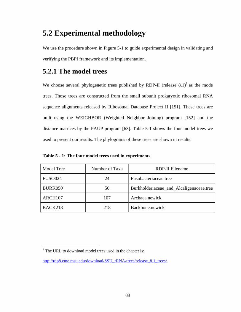
89
5.2 Experimental methodology
We use the procedure shown in Figure 5-1 to guide experimental design in validating and
verifying the PBPI framework and its implementation.
5.2.1 The model trees
We choose several phylogenetic trees published by RDP-II (release 8.1)1 as the mode
trees. Those trees are constructed from the small subunit prokaryotic ribosomal RNA
sequence alignments released by Ribosomal Database Project II [151]. These trees are
built using the WEIGHBOR (Weighted Neighbor Joining) program [152] and the
distance matrices by the PAUP program [63]. Table 5-1 shows the four model trees we
used to present our results. The phylograms of these trees are shown in results.
1 The URL to download model trees used in the chapter is:
http://rdp8.cme.msu.edu/download/SSU_rRNA/trees/release_8.1_trees/.
Table 5 - 1: The four model trees used in experiments Model Tree Number of Taxa RDP-II Filename
FUSO024 24 Fusobacteriaceae.tree
BURK050 50 Burkholderiaceae_and_Alcaligenaceae.tree
ARCH107 107 Archaea.newick
BACK218 218 Backbone.newick
90
5.2.2 The simulated datasets
For each model tree listed in Table 5-1, we choose three numbers of sequence lengths:
1000, 5000, and 10,000. Then for each combination of the model tree and the number of
characters, we simulate 5 datasets under the JC69 model [112] and another 5 datasets
under the K2P model [113] using a sequence simulation program, SEQ-GEN [153]. For
the K2P model, we set the transition/transversion parameters to 2.0. Thus, we simulate a
total of 5 2 3 30× × = datasets for each model tree. We label these datasets using the
model tree name, sequence length, model type and dataset repeat index. For example, the
dataset “back218_L10000_jc69_D003.nex” is the 3rd dataset generated (D003), with a
sequence length of 10,000, under the JC69 model, for the model tree BACK218. To
assess the performance a phylogenetic method statistically, many more datasets may be
needed. However, for validation and verification purposes, the above datasets are
adequate in this dissertation.
5.2.3 The accuracy metrics
There are two issues in choosing the accuracy metrics: 1) quantifying the topological
distance between the estimated tree and the model tree; and 2) summarizing the
simulation results.
In this distance, we use Robinson and Foulds’ measure of topological distance [154].
This distance is equivalent to the number of unique taxon bipartitions found only in one
of the two trees but not both. Chapter 2 illustrates how to calculate bipartitions for a
phylogenetic tree. Taking the model tree as the ground truth, an estimated tree may be
different from the model tree in two ways: it missed some bipartitions included in the
mode tree, or it introduced some novel bipartitions which are not found in the model tree

91
[89]. Missed bipartitions are also called false negative bipartitions, while novel
bipartitions are called false positive bipartitions. When both the model tree and the
estimated tree are fully resolved, the number of false negative partitions equals the
number of false negative partitions, and their sum equals the Robinson and Foulds
topological distance.
For simplicity, we use half of Robinson and Foulds’ distance in our discussions. The
rationales are: 1) there is no biological meaning for this distance; and 2) if the model tree
and the estimated tree has a Robinson and Foulds’ distance of 2, then we can transform
the estimated tree into the model tree with one SPR (Subtree Pruning and Regrafting [77])
move.
The second issue is specific for Bayesian phylogenetic methods because Bayesian-
based methods usually generate a number of tree samples, quite different from other
optimization-based methods. As discussed in Chapter 2, three methods could be used to
summarize these tree samples:
1. The maximum posterior probability tree ( MPPT , the MPP tree): outputting the tree
with the highest frequency of occurrences as an estimate of the true tree.
2. The 95% credible set of trees: outputting the set of trees whose cumulative
occurrence is estimated to be more than 95% of the total number of samples as the
estimation.
3. The majority consensus tree: Calculating the frequencies of each taxa bipartition
and building a consensus tree from the bipartitions whose concurrence
frequencies are above a certain threshold value (for example 50%).

92
In this chapter, we use all these three summary methods and assess the accuracy of
the PBPI based on the following six metrics:
(1) m MPPP(T =T ) : The percentage of the true tree (i.e. the model tree) is recovered as
the MPP Tree.
(2) m CTSP(T T )∉ : The percentage of the true tree (i.e. the model tree) is recovered in
the credible set of trees.
(3) m CONP(T =T ) : The percentage of the true tree (i.e. the model tree) is recovered as
the majority consensus tree.
(4) m MPPd(T ,T ) : The average topological distance between the true tree (i.e. the
model tree) and the MPP tree.
(5) m CTSd(T ,T ) : The average topological distance between the true tree (i.e. the model
tree) and the credible tree set.
(6) m CONd(T ,T ) : The average topological distance between the true tree (i.e. the
model tree) and the majority consensus tree.
In the above metrics, because the 95% credible set may include more than one tree,
we use the smallest distance between the model tree and each individual tree included in
this credible set. If the computed distance equals 0, then the model tree has been found.
5.2.4 Tested programs and their run configurations
We tested PBPI, a software package for parallel Bayesian Phylogenetic Inference that
implements the framework in Chapters 3 and 4. For comparison purposes, we also tested
MrBayes Version 3.1 on part of the dataset.

93
PBPI supports numerous features which can be configured with an XML file. The
configurations of PBPI used in the experiments are given in Table 5-2.
We run PBPI in parallel on 4, 8, or 16 nodes. We use different number of nodes for
different problem sizes to achieve optimal use of CPU time. For each case tested, we run
4 MCMC chains with parallel tempering schema and span each chain on 1, 2, or 4
processors. Each run lasts 1,000,000 generations.
We record both the CPU time (system time + user time) and the wall time on each
node during each run; we use the maximum wall time as the execution time for each run.
We summarize tree samples using metrics provided in Section 5.2.3. We used the
sumt feature provided in PBPI.
In our experiments, we ran sequential versions of MrBayes using the run
configuration given in Figure 5-2. This configuration corresponds to a run with 4 MCMC
chains under JC69 model, each chain lasting 1,000,000 generations.
We did not use the parallel version of MrBayes because doing so has not given any
noticeable execution time change when we run on 1, 2, 4, and 8 processors.
5.2.5 The computing platforms
We run experiments on three systems: NICK at University of South Carolina, DORI in
the SCAPE laboratory at Virginia Tech, and SystemX at Virginia Tech. NICK is a 76-
lset nst=1 rates=equal;
prset statefreqpr=fixed(0.25,0.25,0.25,0.25);
mcmc ngen=1000000 nchains=4 nrun=1 samplefreq=100
printfreq=10000 swapfreq=10;
Figure 5 - 2: Run configuration for MrBayes

94
node Intel Xeon-based dual core cluster, each node having two dual-core 3.2 GHz Intel
Xeon CPUs and a total of 4 GB memory. DORI is an 8-node AMD Opteron-based dual-
core cluster, each node having two dual-code 1.8 GHz AMD Opteron 265 CPUs and a
total of 4GB memory. SystemX is a Terascale computing facility with 1100 Apple
XServer G5 cluster nodes, each node having one Dual 2.3 GHz PowerPC 970FX
processors and 4 GB ECC DDR400 (PC3200) RAM. Though the above three systems
give similar results, we provide the results collected on SystemX because SystemX is a
stable production system.
5.3 Results on model tree FUSO024
5.3.1 The overall accuracy of results
The overall measured accuracy results of PBPI for model tree FUSO024 are shown in
Tables 5-3 and 5-4. In Table 5-3, we show how many times the model tree has been
found as the maximum probability tree (MPP), or the 50% majority consensus tree
(CON), or in the 95% credible set of trees (CTS). In Table 5-4, we show the average
topological distance (½ R-F topological distance) between the model tree and the
estimated trees. The results indicate that the accuracies of PBPI will be improved as more
characters are included in the analysis. Using 10,000 sequences, the model tree has been
found 5 times under the JC69 model (an ideal situation) and 4 times under the K2P model
(some assumption are violated) in all 5 datasets. These results also imply that the 95%
credible set of trees provides better accuracy values than the majority consensus tree and
the maximum probability tree.

95
Table 5 - 2: PBPI run configurations for validation and verification
Parameter Value Meaning
model JC69 Use JC69 as model of evolution
nrun 1 Run once for each dataset
number_of_chains 4 The number of MCMC chains for each run
multipleTry disabled Disable multiple try MCMC feature
sample_interval 1000000 The maximum generations of MCMC chains
maximum_generation 100 How frequently to sample states
print_interval 10000 How frequently to print states
nburnin 0 Start sampling from the beginning
rng1::seed time Use current time as the seed of RNG1
rng2::seed time Use current time as the seed of RNG1
mcmc::bootstrap disabled Disable in-chain MCMC resampling
exchange enabled Enable chain-to-chain exchange
exchange_interval 10 How frequently to perfomr exchange
recombine disabled Disable chain-to-chain recombinations
variablestep disabled Disable variable proposal step
stochasticNNI enabled Enable stochastic NNI proposal
branch enabled Enable stochastic branch proposal
Stochastic SPR enabled Enable stochastic SPR proposal
Stochastic TBR enabled Enable stochastic TBR proposal
Sequence parallel enable Enable sequence level parallism
#chain per group 1 One chain per row on the grid
Chain parallel enabled Enable sequence level parallism
num_partitions 2 Distribute sequences on 2 nodes
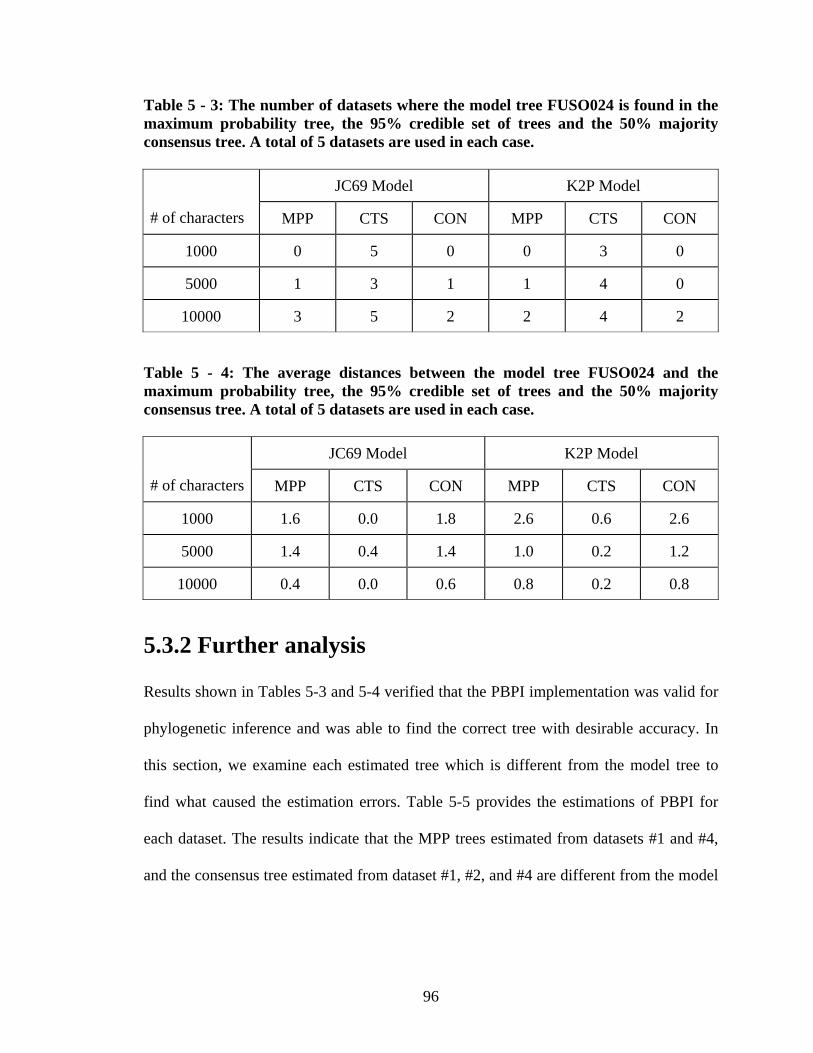
96
5.3.2 Further analysis
Results shown in Tables 5-3 and 5-4 verified that the PBPI implementation was valid for
phylogenetic inference and was able to find the correct tree with desirable accuracy. In
this section, we examine each estimated tree which is different from the model tree to
find what caused the estimation errors. Table 5-5 provides the estimations of PBPI for
each dataset. The results indicate that the MPP trees estimated from datasets #1 and #4,
and the consensus tree estimated from dataset #1, #2, and #4 are different from the model
Table 5 - 3: The number of datasets where the model tree FUSO024 is found in the maximum probability tree, the 95% credible set of trees and the 50% majority consensus tree. A total of 5 datasets are used in each case.
JC69 Model K2P Model
# of characters MPP CTS CON MPP CTS CON
1000 0 5 0 0 3 0
5000 1 3 1 1 4 0
10000 3 5 2 2 4 2 Table 5 - 4: The average distances between the model tree FUSO024 and the maximum probability tree, the 95% credible set of trees and the 50% majority consensus tree. A total of 5 datasets are used in each case.
JC69 Model K2P Model
# of characters MPP CTS CON MPP CTS CON
1000 1.6 0.0 1.8 2.6 0.6 2.6
5000 1.4 0.4 1.4 1.0 0.2 1.2
10000 0.4 0.0 0.6 0.8 0.2 0.8
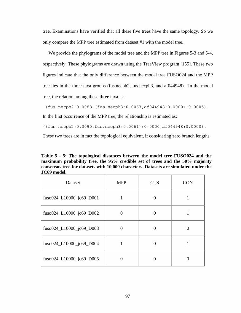
97
tree. Examinations have verified that all these five trees have the same topology. So we
only compare the MPP tree estimated from dataset #1 with the model tree.
We provide the phylograms of the model tree and the MPP tree in Figures 5-3 and 5-4,
respectively. These phylograms are drawn using the TreeView program [155]. These two
figures indicate that the only difference between the model tree FUSO024 and the MPP
tree lies in the three taxa groups (fus.necph2, fus.necph3, and af044948). In the model
tree, the relation among these three taxa is:
(fus.necph2:0.0088,(fus.necph3:0.0063,af044948:0.0000):0.0005).
In the first occurrence of the MPP tree, the relationship is estimated as:
((fus.necph2:0.0090,fus.necph3:0.0061):0.0000,af044948:0.0000).
These two trees are in fact the topological equivalent, if considering zero branch lengths.
Table 5 - 5: The topological distances between the model tree FUSO024 and the maximum probability tree, the 95% credible set of trees and the 50% majority consensus tree for datasets with 10,000 characters. Datasets are simulated under the JC69 model.
Dataset MPP CTS CON
fuso024_L10000_jc69_D001 1 0 1
fuso024_L10000_jc69_D002 0 0 1
fuso024_L10000_jc69_D003 0 0 0
fuso024_L10000_jc69_D004 1 0 1
fuso024_L10000_jc69_D005 0 0 0

98
The above examinations further verified the correctness of PBPI and indicated that
the accuracy measurements shown in Tables 5-3 and 5-4 can be increased significantly
once the zero branch factors are included in the topological distance calculation.
0.1
fus.gonidi
fus.necph2
fus.necph3
af044948
fus.russi
fus.simiae
fus.nuclea
aj006965
fus.nucle7
fus.perfoe
af189244
lpt.bucca2
sbd.termit
stb.monili
stb.monil2
lpt.microb
x83517
cb.ceti1
prg.modest
prg.maris
fus.varium
fus.mortif
c.rectum
fus.morti3
Figure 5 - 3: The phylogram of the model tree FUSO024

99
0.1
fus.gonidi
af044948
fus.necph2
fus.necph3
fus.russi
fus.simiae
fus.nuclea
aj006965
fus.nucle7
fus.perfoe
af189244
lpt.bucca2
sbd.termit
stb.monili
stb.monil2
lpt.microb
x83517
cb.ceti1
prg.modest
prg.maris
fus.varium
fus.mortif
c.rectum
fus.morti3
Figure 5 - 4: The MPP tree estimated from dataset fuso024_L10000_jc69_D001

100
5.3.3 PBPI stability
The above accuracy results are obtained from a single run for each given dataset. To
demonstrate that PBPI will produce stable estimations, we examined 10 individual runs
on the dataset fuso024_L10000_jc69_D001. The resulted topological distances between the
model tree and the three summarized trees are show in Figure 5-5 where the x-axis is the
index of each run, and y-axis is the ½ R-F topological distance. To show that the stability
will not be affected by the number of processors, the first 5 runs were on 4 processors and
the second 5 runs were on 8 processors. The results show that 8 runs obtained the same
estimation while the other 2 runs have estimated one different branch. As discussed in
Section 5.3.2, the topological distance shown here should be corrected by including the
zero branch length into the topological calculation. After the correction, all 10 trees are
equivalent to the model tree. These empirical results confirm that the estimations
obtained from PBPI are stable.
PBPI Estimation Stability
0
0.5
1
1.5
2
2.5
0 1 2 3 4 5 6 7 8 9 10
Index of Runs
Topo
logi
cal D
ista
nce
MPPCTSCON
Figure 5 - 5: Estimation variances in 10 individual runs
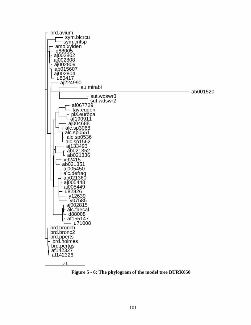
101
0.1
brd.aviumsym.blcrcu
sym.critspamo.xyldend88005
aj002802aj002808aj002809ab015607aj002804u80417
aj224990lau.mirabi
ab001520sut.wdswr3sut.wdswr2
af067729tay.eqgenipls.europaaf190911
aj004688alc.sp3068alc.sp0551alc.sp0536alc.sp1562aj133493ab021352ab021336
x92415ab021351aj005450alc.defragab021360aj005448aj005449u82826
y12639y07585
aj002815alc.faecald88008af155147
u71008brd.bronchbrd.bronc2brd.ppertsbrd.holmesbrd.pertusaf142327af142326
Figure 5 - 6: The phylogram of the model tree BURK050
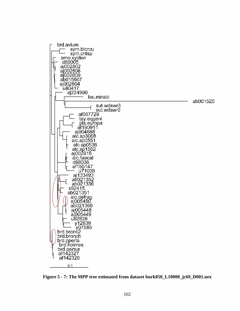
102
Figure 5 - 7: The MPP tree estimated from dataset burk050_L10000_jc69_D001.nex

103
5.4 Results on model tree BURK050
In Table 5-6, we show how many times the model tree BURK050 was found as the
maximum probability tree (MPP), or the 50% majority consensus tree (CON), or in the
95% credible set of trees (CTS). The results indicated that the accuracy could be
improved as more characters were included in the analysis. After correcting the zero
branch lengths problem, we concluded that PBPI is a consistent phylogenetic method.
The model tree of BURK050 and the maximum probability tree estimated from
the dataset burk050_L10000_jc69_D001.nex by PBPI are provided in Figures 5-6 and 5-7.
This MPP tree had three bipartitions different from the model tree. The locations of those
differences are circled in Figure 5-7. All of them were the artifacts of the R-F distance
metric because it takes no account of zero or near-zero branch lengths.
Table 5 - 6: The average distances between the model tree BURK050 and the maximum probability tree, the 95% credible set of tree and the 50% majority consensus tree. A total of 5 datasets were used in each case.
JC69 Model K2P Model
# of characters MPP CTS CON MPP CTS CON
1000 20.8 4.2 13.4 24 4 13.2
5000 5.2 1.6 6.6 5.6 1.2 6.2
10000 3 0.8 4.2 3.4 0.4 4

104
The summary of tree samples includes 625 trees in the 95% credible tree sets, most of
which had at most 5 partitions different from the model tree. The posterior probability
value of the MPP tree in the examined dataset was about 0.6%. The posterior
probabilities of the first 50 trees in the credible set are shown in Figure 5-8. The
“uncorrected” (see discussion in Section 5.3.2) topological distance distributions of these
trees are shown in Figure 5-9. These two figures indicate that PBPI have the capability to
find multiple statistical equivalent trees which are close to the model tree. However, as
we only use one model tree to generate the data, we need some insightful interpretations
for the posterior probabilities of these tree samples.
Probability Distribution of the Top 50 Most Probable Trees
0
0.001
0.002
0.003
0.004
0.005
0.006
0.007
0 5 10 15 20 25 30 35 40 45 50
Index of the Trees
Prob
abili
ty A
prro
xim
ated
Fro
m T
ree
Sam
ples
Figure 5 - 8: The posterior distribution of the top 50 most probable trees

105
5.5 Chapter summary
In this chapter, we validated the correctness of PBPI implementation and measured its
accuracy using simulation study. We randomly chose several phylogenetic trees
published by RDP-II project as the model trees. We simulated a group of datasets with
different numbers of characters under the JC69 and K2P models and analyzed these
datasets using PBPI. The experimental results showed that PBPI estimated the correct
trees or equivalent trees for all datasets with 10,000 characters. Thus we concluded that
PBPI was both correct and consistent for inferring phylogeny under ideal situations.
The results also indicated that when part of the assumptions were violated (for
example, there was a transition and transversion bias in the simulated data), PBPI still
achieved estimations which were very close to the model trees.
Topological Distances between the Model Tree and the Top 50 Most Probable Trees
0
1
2
3
4
5
6
0 5 10 15 20 25 30 35 40 45 50
Index of the Trees
Topo
logi
cal D
ista
nce
Figure 5 - 9: The topological distances distribution of the top 50 most probable trees

106
We provided detailed results on the model trees FUSO024 and BURK050. Multiple
runs on the same dataset indicated that PBPI produced stable estimations, though the
method itself was a stochastic algorithm.
We also showed the probability distributions and topological distance distributions of
the first 50 trees in the credible tree sets. The results demonstrated the possibility that
there were multiple, statistically-equivalent phylogenetic trees for the same dataset; this
signified a potential advantage of Bayesian methods over other optimization-based
methods which produce only one tree as the estimation.
We measured execution time of both PBPI and MrBayes; the results presented in
Chapter 6 showed that for the same dataset and similar run configurations, PBPI ran
much faster than MrBayes, both in sequential and in parallel. On a product HPC system,
SystemX, PBPI reduced the execution time 5~10 times running on a single node mode,
and hundreds of times when running on 32 nodes.
Our experiments also showed a couple of issues with MCMC-based Bayesian
phylogenetic inference, including constraints caused by limited numeric precision in
floating point number representation and the failure of Metropolis-coupled MCMC to
infer large phylogenies (>500 taxa). These limitations call for further improvement of
Bayesian polygenetic inference and we leave them as future work.

107
Chapter 6
Performance Evaluation
6.1 Introduction
In Chapter 5, we provided verification and accuracy measurements of our PBPI
implementation. In this chapter we further evaluate the computational performance of
PBPI. As discussed in Chapter 4, the computational performance of PBPI is studied with
parallel speedup and scalability.
The performance of a parallel algorithm is measured by speedup or efficiency. The
speedup of a parallel algorithm using p processors is defined as
)(
)( 0
pTT
pSP
= (6- 1)
Here 0T is the running time of the fastest known sequential algorithm on one processor
for the same problem.
There are a number of possibilities for timing analysis, and different methods will
give disparate results. Figure 6-1 shows the different values under different timing
methods (user time versus wall time) for the same example. In this paper, we chose the
wall clock time, that is, the elapsed time between the start and the end of a specific run.

108
Wall clock time will make the speedup smaller than that computed with other timing
methods, such as user time. However, wall clock time includes such negative effects as
communication overhead, idle time caused by imbalance, and synchronization. One
disadvantage of using wall clock time to measure speedup is that the same program may
give different results in a non-dedicated environment.
Speedup computed by wall clock time and user time
0
5
10
15
20
25
30
35
0 4 8 12 16 20 24 28 32Number of Processors
Spee
dup
Wall clock timeUser time
Figure 6 - 1: Different speedup values computed by wall clock time and user time
6.2 Experimental methodology
We evaluated the implementation of PBPI in a Terascale Computing Facility, SystemX,
at Virginia Tech. This system has 1100 Apple XServer G5 cluster nodes, each node
having one Dual 2.3 GHz PowerPC 970FX processors, and 4 GB ECC DDR400 (PC3200)
RAM. The cluster nodes were connected with SilverStorm’s 91200 InfiniBand-based
switches with a bidirectional port speed of 10 Gbps (billions of bits per second).

109
We used a subset of the datasets described in Chapter 5 as the benchmark datasets for
performance evaluations. Given each model tree, we generated two datasets, each having
1000 and 10,000 characters. These datasets are listed in Table 6-1.
We analyzed the benchmark datasets under the JC69 model. We set the maximum
generations for the MCMC run at 200,000. All other analysis configurations were the
same as those used in Chapter 5.
In our evaluation, we benched the execution time of the sequential version of PBPI
and MrBayes using the same dataset on a single node. Then we profiled the execution
time of PBPI running in parallel mode and calculated the speedup values under various
run settings (different numbers of processors, different grid topologies, and different
problem sizes).
To get the performance data, we executed 5 runs for each case. The average execution
time over 5 runs was used to compute the speedup. Since PBPI is a stochastic algorithm,
we also showed the variance of all measured numbers. We used wall clock time in timing
Table 6 - 1: Benchmark dataset used in the evaluation
Dataset # of data # of characters # of pattern
FUSO024_1000 24 1000 402
FUSO024_10000 24 10000 1972
BURK050_1000 50 1000 432
BURK050_10000 50 10000 2429
ARCH107_1000 107 1000 1000
ARCH107_10000 107 10000 9996
BACK218_1000 218 1000 1000
BACK218_10000 218 10000 10000

110
analysis. For parallel executions, as each node may take different execution time, we used
the recorded maximum values of execution time for all evaluations.
6.3 The sequential performance of PBPI
Since MrBayes is one of the most widely used Bayesian phylogenetic inference programs,
we compared the performance of PBPI against MrBayes. The version of MrBayes we
have tested was Version 3.1.
6.3.1 The execution time of PBPI and MrBayes
Table 6-2 provides the profiled execution time of PBPI and MrBayes on the benchmark
dataset running in a single node on SystemX. The measured results indicated that when
both programs run in sequential mode, PBPI runs 5~19 times faster than MrBayes,
depending on the problem size. The larger the problem size, the larger performance
improvement of PBPI over MrBayes. Also, as the table shows, the variances are less than
Table 6 - 2: Sequential execution time of PBPI and MrBayes
Dataset TPBPI
(Second) TMrBayes
(Seconds) S = TMrBayes / TPBPI
fuso024_L1000 102.8±2.2 605.4±0.3 5.8±2%
fuso024_L10000 563±28 2765.2±1.6 4.7±5%
burk050_L1000 169.8±4.8 1403.3±0.5 8.0±3%
burk050_L10000 903.2±56.2 7257.0±28.1 7.5±6%
arch107_L1000 643.2±33.8 6796.5±10.5 10.0±5%
arch107_L10000 6407.6±346.4 66130.7±145.2 9.8±5%
back218_L1000 836.0±41.0 13913.5±20.5 15.8±5%
back218_L10000 7978.8±197.0 156233.3±333.3 19.1±3%

111
6% during our experiments. We credited this performance increase to improved memory
management and local update schema in likelihood calculation.
6.3.2 The quality of the tree samples drawn by PBPI
Since PBPI uses different implementation than MrBayes, and since both algorithms are
stochastic algorithms, an important concern is raised about the quality of the MCMC
samples. In other words, was the quality of MCMC samples drawn by PBPI as good as
the samples drawn by MrBayes?
We answered such questions in two ways. First, we compared the log likelihood plots
of both programs. Second we compared the summary of both tree samples.
Figure 6-2 plots the log likelihood of the tree samples for the dataset FUSO024_1000
drawn in the first 5000 generations by PBPI and MrBayes. Both programs reached the
same level of stationary equilibrium at about the same time. This plot demonstrated that
tree samples drawn by PBPI and MrBayes were similar.
The consensus trees, with posterior probability of each bipartition summarized from
Log Likelihood Plot of MCMC Samples
0
2000
4000
6000
8000
10000
12000
0 1000 2000 3000 4000 5000Generations
-lnL
PBPIMrBayes
Figure 6 - 2: Log likelihood plot of the tree samples drawn by PBPI and MrBayes
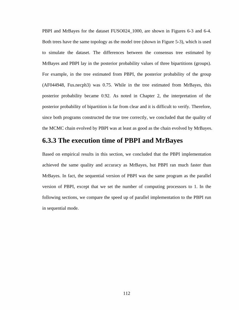
112
PBPI and MrBayes for the dataset FUSO024_1000, are shown in Figures 6-3 and 6-4.
Both trees have the same topology as the model tree (shown in Figure 5-3), which is used
to simulate the dataset. The differences between the consensus tree estimated by
MrBayes and PBPI lay in the posterior probability values of three bipartitions (groups).
For example, in the tree estimated from PBPI, the posterior probability of the group
(AF044948, Fus.necph3) was 0.75. While in the tree estimated from MrBayes, this
posterior probability became 0.92. As noted in Chapter 2, the interpretation of the
posterior probability of bipartition is far from clear and it is difficult to verify. Therefore,
since both programs constructed the true tree correctly, we concluded that the quality of
the MCMC chain evolved by PBPI was at least as good as the chain evolved by MrBayes.
6.3.3 The execution time of PBPI and MrBayes
Based on empirical results in this section, we concluded that the PBPI implementation
achieved the same quality and accuracy as MrBayes, but PBPI ran much faster than
MrBayes. In fact, the sequential version of PBPI was the same program as the parallel
version of PBPI, except that we set the number of computing processors to 1. In the
following sections, we compare the speed up of parallel implementation to the PBPI run
in sequential mode.

113
Figure 6 - 3: The consensus tree estimated by PBPI
0.1
Fus.gonidi
Fus.necph2
Fus.necph3
AF0449480.75
1.00
Fus.russi
Fus.simiae
Fus.nuclea
AJ006965
Fus.nucle71.00
0.58
1.00
1.00
Fus.perfoe
AF189244
Lpt.bucca21.00
Sbd.termit
Stb.monili
Stb.monil21.00
Lpt.microb
X835171.00
1.00
0.98
1.00
Cb.ceti1
Prg.modest
Prg.maris1.00
1.00
1.00
Fus.varium
Fus.mortif
C.rectum
Fus.morti31.00
1.00
1.00
1.00
1.00

114
0.1
Fus.gonidi
Fus.russi
Fus.simiae
Fus.nuclea
AJ006965
Fus.nucle71.00
0.80
1.00
1.00
Fus.perfoe
AF189244
Lpt.bucca21.00
Sbd.termit
Stb.monili
Stb.monil21.00
Lpt.microb
X835171.00
1.00
0.94
1.00
0.54
Cb.ceti1
Prg.modest
Prg.maris1.00
1.00
1.00
Fus.varium
Fus.mortif
C.rectum
Fus.morti31.00
1.00
1.00
1.00
1.00
Fus.necph2
Fus.necph3
AF0449480.92
1.00
Figure 6 - 4: The consensus tree estimated by MrBayes

115
6.4 Parallel speedup for fixed problem size
We used benchmark datasets FUSO024_10000, ARCH107_1000, and BACK218_10000
as fixed problems to investigate the parallel speedup of PBPI. These three datasets
represented three kinds of problems:
• FUSO024_10000: problems with a small number of taxa and long sequences of
characters;
• ARCH107_1000: problems with a medium number of taxa and short sequences
of characters;
• BACK218_10000: problems with a large number of taxa and long sequences of
characters.
For each dataset, we ran 4 chains with parallel tempering schema, each chain lasting
200,000 generations. We scale the number of processors from 4 to 64 and calculate the
average, maximum, and minimum values of the speedup. The results are shown in
Figures 6-5, 6-6, and 6-7.
The results indicated that for all three benchmark datasets, PBPI achieved roughly
linear speedup, with measurement errors ranging from -16% to 12%. For
FUSO024_L10000 dataset, the maximum speedup was 28.1 and the minimum speedup
was 25.6 when using 64 nodes. For ARCH107_L1000 dataset, the maximum speedup
was 24.7 and minimum speedup was 23.0 when using 64 nodes. For Back218_L10000
dataset, the maximum speedup was 50.6 and minimum speedup was 43.6 when using 64
nodes. We also observed that when using small number of processors (<8), the
ARCH107_L1000 dataset had a larger speedup than the FUSO024_L10000 dataset.
When the number of processors was increased, this observation reversed.

116
Combining the performance improvement both in sequential optimization and parallel
speedup, for the same dataset, PBPI ran up to 874 times faster using 64 processors than
MrBayes using a single processor on a system similar to SystemX.
To demonstrate that PBPI running in parallel mode would generate statistically
equivalent tree samples, we summarized the tree samples output by parallel MCMC runs
and compared them with the ground truth: the model tree. The results matched our
informal proof in Chapter 5 and the simulation study in Chapter 6. Figure 6-8 shows the
tree estimated using 64 processors. After one re-rooting operation (which does not
change the tree topology from when the tree is unrooted), the only difference between the
estimated tree and the model tree was that the subtree (Fus.necph2, (Fus.necph3,
AF04948)) in the model tree became ((Fus.necph2, Fus.necph3), AF04948). Since, the
tree edge between AF04948 and (Fus.necph2, Fus.necph3) had zero lengths in both trees;
these two trees were the same.
Parallel Speedup of PBPI for Dataset FUSO024_L10000
0
5
10
15
20
25
30
4 8 16 32 64
Number of Processors
Spee
dup
AverageMaximumMinmum
Figure 6 - 5: Parallel speedup of PBPI for dataset FUSO024_L10000

117
Parallel Speedup of PBPI for Dataset: ARCH107_L1000
0
5
10
15
20
25
30
4 8 16 32 64
Number of Processors
Spee
dup
AverageMaximumMinmum
Figure 6 - 6: Parallel speedup of PBPI for dataset ARCH107_L1000
Parallel Speedup of PBPI for Dataset BACK218_L10000
0
10
20
30
40
50
60
4 8 16 32 64
Number of Processors
Spee
dup
AverageMaximumMinmum
Figure 6 - 7: Parallel speedup of PBPI for dataset BACK218_L10000
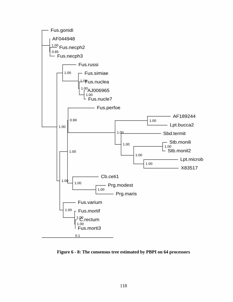
118
0.1
Fus.gonidi
AF044948
Fus.necph2
Fus.necph30.85
1.00
Fus.russi
Fus.simiae
Fus.nuclea
AJ006965
Fus.nucle71.00
1.00
1.00
1.00
Fus.perfoe
AF189244
Lpt.bucca21.00
Sbd.termit
Stb.monili
Stb.monil21.00
Lpt.microb
X835171.00
1.00
1.00
1.00
0.99
Cb.ceti1
Prg.modest
Prg.maris1.00
1.00
1.00
Fus.varium
Fus.mortif
C.rectum
Fus.morti31.00
1.00
1.00
1.00
1.00
Figure 6 - 8: The consensus tree estimated by PBPI on 64 processors

119
6.5 Scalability analysis
Before we discuss the scaled parallel speedup and impacts of grid topology, we will
analyze scalability of PBPI using equation (4-5). The workload of sequential MCMC
algorithms (without considering memory latency in this section) is approximately
0 1 2 3logotherlocal update global update TT T
W T k hm n k hmn k− −
= ≈ + + . (6- 2)
Here, ik , for 1,...,3i = is constant, n is the number of taxa, m is the number of
characters patterns, and h is the number of chains. Similarly, the computation time of
the parallel MCMC algorithm can be approximated as
2 31
5 64
1 24 5
6 3 7
( log )( ) log log
log
p
T TT
T TT
k hm n k hmn cp hT p k kp h c
k m n k k
+≈ + +
+ + +. (6- 3)
Here, ik for 1,...,7i = , is constant, p is the number of processors, and c is the number of
chains per row. The terms in the right part of this equation represent real computation
time ( 1T ), row collective communication time ( 2T ), column collective communication
time ( 3T ), imbalance overhead ( 4T ), sequential overhead ( 5T ), and parallel overhead ( 6T ),
respectively. The speedup of the parallel algorithm can be predicted as
( )
( )4 5 6 3 7
1 2 3
1( , , ; ) .log log log
1og / /
S n m h p pcp hk k k m n k k
p h chmn k l n n k k hmn
⎛ ⎞⎜ ⎟⎜ ⎟⎜ ⎟≈ ⎜ ⎟⎛ ⎞ ⎛ ⎞⎜ ⎟+ + + +⎜ ⎟ ⎜ ⎟
⎝ ⎠ ⎝ ⎠⎜ ⎟+ ⋅⎜ ⎟+ +⎝ ⎠
(6- 4)

120
From equation (6-4), we make the following observations:
1) The problem size (W ) is determined by n , m , and h . According to equation (6-4),
the larger the problem size, the bigger the speedup that can be obtained.
2) It is possible to remove the column collective communication overhead (i.e.,
4 log cpkh
⎛ ⎞⎜ ⎟⎝ ⎠
is decreased), and row collective communication overhead 5 log hkc
⎛ ⎞⎜ ⎟⎝ ⎠
is
decreased, since no row collective communication is needed in swap step). We
discussed three chain swapping algorithms in an earlier paper [156]. Our analysis and
empirical results indicate that
3) Communication overhead ( 4 5log logcp hk kh c
⎛ ⎞ ⎛ ⎞+⎜ ⎟ ⎜ ⎟⎝ ⎠ ⎝ ⎠
) and imbalance ( ( )6 logk m n ) are
major factors that influence performance scalability. For a small problem size,
communication overhead is important. For a larger problem size, imbalance is the
major obstacle.
4) Assume we have synchronized the proposal types using RNG-2 and also balanced the
tree through tree re-root operation. Then the imbalance overhead is mainly caused by
the sample mean of multiple random samples from (0, log )U n . This means small
exchange steps result in large imbalance. One way to reduce imbalance overhead is to
enlarge exchange step. Another way is to use asymmetric algorithms to decouple the
interaction of different chains.
5) When p and h are fixed, running more chains for each row may result in larger
column size and thus larger row communication overhead.

121
6.6 Parallel speedup with scaled workload
With a fixed problem size, parallel speedup will finally slow down as the number of
processors reaches some threshold. After that point, there is no further performance gain
from using more processors. This limitation is governed by Amdahl’s law [143].
However, additional speedup can be obtained by scaling the problem size. Though
speedup obtained from scaling problem size will not reduce the execution time further, it
does have the advantage of improving the accuracies and precisions of the solution.
As implied in equation (6-4), we can scale the Bayesian phylogenetic inference
problem size in three dimensions: 1) the number of taxa; 2) the number of characters; and
3) the number of MCMC chains. Though it is an interesting problem, how the results of
Bayesian phylogenetic inference are affected by scaling the problem in these three
dimensions is beyond the scope of this dissertation. In this section, we focus on the
impact of the problem size on the speedup achieved by PBPI.
6.6.1 Scalability with different problem sizes
The speedup curves of PBPI for datasets FUSO024_L10000, ARCH107_1000, and
BACK218_L10000 are shown in Figure 6-9.
As shown in Chapter 2, the amount of computation required in likelihood evaluation
is proportional to the number of unique site patterns (or the number of characters);
increasing the number of characters linearly increases the execution time. Equation (6-4)
indicates that speedup scales with the number of characters very well. On the other hand,
increasing the number of taxa only increases the computation at the rate of log N (where
N is the number of taxa). Thus, though the number of taxa in dataset FUSO024_L10000
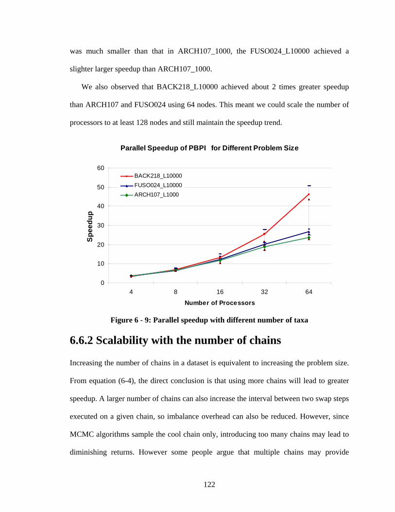
122
was much smaller than that in ARCH107_1000, the FUSO024_L10000 achieved a
slighter larger speedup than ARCH107_1000.
We also observed that BACK218_L10000 achieved about 2 times greater speedup
than ARCH107 and FUSO024 using 64 nodes. This meant we could scale the number of
processors to at least 128 nodes and still maintain the speedup trend.
Parallel Speedup of PBPI for Different Problem Size
0
10
20
30
40
50
60
4 8 16 32 64
Number of Processors
Spee
dup
BACK218_L10000FUSO024_L10000ARCH107_L1000
Figure 6 - 9: Parallel speedup with different number of taxa
6.6.2 Scalability with the number of chains
Increasing the number of chains in a dataset is equivalent to increasing the problem size.
From equation (6-4), the direct conclusion is that using more chains will lead to greater
speedup. A larger number of chains can also increase the interval between two swap steps
executed on a given chain, so imbalance overhead can also be reduced. However, since
MCMC algorithms sample the cool chain only, introducing too many chains may lead to
diminishing returns. However some people argue that multiple chains may provide

123
multiple starting points to explore the tree space. Further experiments are needed to
justify which argument is true.
6.7 Chapter summary
In this chapter, we presented experimental evaluation of the parallel performance of PBPI
on a Terascale computing system, SystemX. Comparing PBPI with MrBayes in
sequential mode, using different benchmark datasets, showed that PBPI runs 5~19 times
faster than MrBayes and achieves similar results as well. We measured the speedup of
PBPI on several benchmark datasets on SystemX; it achieved roughly linear speedup
when using 4 to 64 processors. This lack of slowdown indicated that PBPI has the
capability to scale up to hundreds of processors.
The memory space was distributed in our algorithms; the duplicated data was limited
primarily to the input dataset, which was relatively small compared with the data likely to
be encountered in ongoing modeling. Our algorithms could make inferring large
phylogenies—which require huge memory space and compute cycles—feasible and fast.
Combining both sequential and parallel speedup, PBPI may run 874 times faster than
MrBayes (version 3.1), even only using 64 nodes. PBPI also exploits parallelism at the
bootstrapping and dataset levels. This means Bayesian phylogenetic inference, which
takes several months to complete, now can be finished in less than a half day. This
performance improvement makes large scale investigation of Bayesian phylogenies a
reality.
In future work, we will extend PBPI to support more evolutionary models of new
data types.

124
Chapter 7
Summary and Future Work
7.1 The big picture
In this work, we studied and extended the framework of Bayesian phylogenetic inference
using Markov Chain Monte Carlo (MCMC) methods. Bayesian analysis is of interest to
scientists in fields including biology, statistics, and computer science. Various issues
have been identified for current Bayesian phylogenetic inference methods and
implementations:
1) As the evolutionary process happens only once, there is only one phylogenetic tree
corresponding to the evolutionary process for a group of taxa. This concept has been
held among biologists for a long time. A convincing interpretation of Bayesian
posterior probability of phylogenetic models within a biological and statistical context
is therefore required.
2) Most, if not all, Bayesian phylogenetic inferences use an MCMC method to generate
samples from the posterior distribution which is in a complex, high dimensional space.
The previous MCMC methods may fail accurately to explore the posterior
distribution due to slow convergence, high stickiness, and local optima phenomena.

125
3) MCMC methods are computationally expensive. A comprehensive Bayesian
phylogenetic inference of hundreds of taxa under complex evolutionary models may
take months to finish. This disadvantage limits the application of Bayesian
phylogenetic inference to very large phylogenetic problems and also hinders further
investigations of the behavior of Bayesian phylogenetic inference methods.
4) Discrepancies between the confidence support values obtained from Bayesian
phylogenetic inference and those values obtained from traditional phylogenetic
methods are highly debatable. Without identifying the inherent causes of such
discrepancies, there is little justification for preferring one method over the other. It is
even worse to dispute one method using a conclusion drawn from the other method
but without acknowledging that different assumptions are being used by the two
methods.
5) The increasing size of datasets is making a grand challenge of Bayesian phylogenetic
inference. Phylogenetic analysis of tens of thousands of taxa with hundreds of genes
may deepen our understanding about biological evolution and diversity. Such
phylogenetic analyses are better conducted within a statistically sound probabilistic
framework that has the ability to incorporate existing knowledge and comprehensive
models. Bayesian analysis is promising, but some breakthroughs are needed to make
it practical.
Our work attempts to provide solutions for some of the above issues through various
efforts:
1) For the correct interpretation of Bayesian posterior probability of phylogenetic
models, we revisited the Bayesian phylogenetic inference framework and reviewed

126
different options for Bayesian phylogenetic methods. We found that the Bayesian
posterior probability distribution of phylogenetic models is highly correlated to the
likelihood ranking of these models. The likelihood ratio of two phylogenetic models
roughly equals to the posterior probability ratio of these two models. Therefore, the
posterior probability of a phylogenetic model reflects the probability that the data are
supported by this model.
2) To make MCMC methods more robust and more efficient, we proposed several
extended tree mutation operators which vary the step length to explore larger region of
the phylogenetic model state space. We also studied several MCMC strategies for
Bayesian phylogenetic inference that can effectively increase the mixing rate of the
MCMC chains, making the chains converge faster with less danger of being trapped in
regions separated by a high energy barrier.
3) To reduce the computation time of current Bayesian analysis and make Bayesian
phylogenetic inference feasible for solving large phylogenies which need long
computation time and have large memory requirements, we developed and implemented
PBPI as a high performance implementation of the Bayesian phylogenetic inference
method. The PBPI code can run on a wide range of parallel computing platforms.
4) Using a simulation study, we measured the accuracy of PBPI on several model trees
with different number of taxa. The empirical results show that PBPI is a consistent
phylogenetic method which can, given enough data, .estimate all non-zero length
branches correctly.
5) We also evaluated the performance of PBPI and compared it with MrBayes, one of
the leading Bayesian phylogenetic inference program. In sequential mode, PBPI runs up
127
to 19 times faster than MrBayes for some of our tested datasets. In parallel mode, PBPI
achieves an average 46× speedup on 64 processors. Results also indicate PBPI have the
capability to scale up to hundreds of processors given a proper problem size.
6) To further resolve the discrepancies between Bayesian posterior probability and
Bootstrap support value, we introduce in-chain resampling MCMC (IR-MCMC) methods
which combine data uncertainty and model uncertainty into a single confidence support.
Our analysis clarifies some misleading explanations about the Bootstrap support and
Bayesian posterior probability. The experimental results indicate that IR-MCMC can
capture the data variance existed in the input dataset and include data uncertainties into
an extended version of Bayesian posterior probability.
In this research, we developed open-source software which will be made available to
the public for use in further research. Though this work is focused on Bayesian
phylogenetic inference, many ideas in this work are general and can be applied in solving
other problems.
7.2 Future work
This work is only the first step in building a comprehensive framework. In follow-on
work, we hope to extend this framework as follows:
1) Analyzing the performance of Bayesian phylogenetic methods more thoroughly
through theoretical and experimental study. We may need to develop a set of benchmark
datasets and models for performance analysis. We also need to run the benchmark under
an HPC environment and automate the benchmarking process. Considering the increasing
interest in Bayesian phylogenetic inference but insufficient investigation of the
128
performance of this method, a more comprehensive study of Bayesian phylogenetic
inference could clarify some confusions.
2) Developing a more robust, effective MCMC framework to support advanced
Bayesian analysis. There is no evidence to show that Metropolis-coupled MCMC always
approximates the posterior distribution correctly.
3) Extending Bayesian analysis to support more data types and models. As a general
statistical framework, the Bayesian approach has the potential to solve phylogenetic
problems in which uncertainties exist and need to be accommodated. In addition to
dealing with complex models for DNA sequences, Bayesian analyses can be used to
handle novel data types such as gene order [75] and genome contents [72-74, 166].
4) Developing a formal framework to assemble subtrees generated in Bayesian analysis
to a supertree with confidence support on each clade. One advantage of Bayesian analysis
is that the inference always provides measures of clade support. However, current
supertree approaches do not use such information.
5) To resolve the discrepancies between Bayesian posterior probability and bootstrap
support values, we extended Bayesian phylogenetic inference to include both
uncertainties and proposed using IR-MCMC (in-chain resampling MCMC) to estimate
the effects of both data uncertainty and model uncertainty. The experimental results
indicate that IR-MCMC can include data uncertainties into an extended version of
Bayesian posterior probability. As a future work, we need more thorough theoretical and
experimental investigations of the IR-MCMC method.

129
Bibliography
[1] Hillis, D. M., "Biology Recapitulates Phylogeny," Science, vol. 276, pp. 218-219,
1997.
[2] NSF, "Assembling the Tree of Life (ATOL)," 2003.
[3] Owen, R. J., "Helicobacter - species classification and identification," British
Medical Bulletin, vol. 54, pp. 17-30, 1998.
[4] Pennisi, E., "Modernizing the Tree of Life," Science, vol. 300, pp. 1692-1697,
2003.
[5] Graur, A.G,. and Li, W.-H., Fundmentals of Molecular Evolution. Sunderland,
MA: Sinauer, 1991.
[6] Eisen, J. A. and Fraser, C. M., "Phylogenomics: Intersection of Evolution and
Genomics," Science, vol. 300, pp. 1706-1707, 2003.
[7] Nichol S. T., Spiropoulou C. F., Morzunov S, Rollin P. E., Ksiazek T. G.,
Feldmann H, Sanchez A, Childs J, Zaki S, Peters C. J., "Genetic identification of
a hantavirus associated with an outbreak of acute respiratory illness," Science in
China Series F-Information Sciences, vol. 262, pp. 914-917, 1993.
[8] Murphy, W. J., Eizirik, E., O'Brien, S. J., et al., "Resolution of the Early Placental
Mammal Radiation Using Bayesian Phylogenetics," Science, vol. 294, pp. 2348-
2351, 2001.
[9] Webster, A. J., Payne, R. J. H., and Pagel, M., "Molecular Phylogenies Link Rates
of Evolution and Speciation," Science, vol. 301, pp. 478-, 2003.

130
[10] Huelsenbeck, J. P., Ronquist, F., Nielsen, R., et al., "Bayesian Inference of
Phylogeny and Its Impact on Evolutionary Biology," Science, vol. 294, pp. 2310-
2314, 2001.
[11] Venter, J. C., Adams, M. D., Myers, E. W., et al., "The Sequence of the Human
Genome," Science, vol. 291, pp. 1304-1351, 2001.
[12] Benson, D. A., Karsch-Mizrachi, I., Lipman, D. J., et al., "GenBank," Nucl. Acids
Res., vol. 33, pp. D34-38, 2005.
[13] Stoesser, G., Baker, W., Van Den Broek, A., et al., "The EMBL Nucleotide
Sequence Database," Nucl. Acids Res., vol. 30, pp. 21-26, 2002.
[14] Tateno, Y., Miyazaki, S., Ota, M., et al., "DNA Data Bank of Japan (DDBJ) in
collaboration with mass sequencing teams," Nucl. Acids Res., vol. 28, pp. 24-26,
2000.
[15] Bairoch, A. and Apweiler, R., "The SWISS-PROT protein sequence database and
its supplement TrEMBL in 2000," Nucl. Acids Res., vol. 28, pp. 45-48, 2000.
[16] NSF, "Tree of Life Workshop III: Developing the Technology and Infrastructure
Needed for Assembling the Tree of Life," University of Texas, Austin December
2000.
[17] Li, W.-H., Molecular Evolution. Sunderland, MA: Sinauer Associates, 1997.
[18] Lio, P. and Goldman, N., "Models of Molecular Evolution and Phylogeny,"
Genome Res., vol. 8, pp. 1233-1244, 1998.
[19] Giribet, G. and Wheeler, W. C., "On Gaps," Molecular Phylogenetics and
Evolution, vol. 13, pp. 132-143, 1999.

131
[20] Wheeler, W., "Optimization alignment: the end of multiple sequence alignment in
phylogenetics?," Cladistics, vol. 12, pp. 1-9, 1996.
[21] Felsenstein, J., "Taking Variation of Evolutionary Rates Between Sites into
Account in Inferring Phylogenies," Journal of Molecular Evolution, vol. 53, pp.
0447-0455, 2001.
[22] Lunter, G., Miklos, I., Drummond, A., et al., "Bayesian phylogenetic inference
under a statistical insertion-deletion model," in Algorithms in Bioinformatics,
Proceedings, vol. 2812, Lecture Notes in Bioinformatics. Berlin: Springer-Verlag
Berlin 2003, pp. 228-244.
[23] Durbin, R., Eddy, S., Krogh, A., et al., Biological Sequence Analysis:
Probabilistic Models of Proteins and Nucleic Acids: Cambridge University Press,
1998.
[24] Robinson, D. M., Jones, D. T., Kishino, H., et al., "Protein evolution with
dependence among codons due to tertiary structure," Molecular Biology and
Evolution, vol. 20, pp. 1692-1704, 2003.
[25] Nylander, J. A. A., Ronquist, F., Huelsenbeck, J. P., et al., "Bayesian
phylogenetic analysis of combined data," Systematic Biology, vol. 53, pp. 47-67,
2004.
[26] Buckley, T. R., Arensburger, P., Simon, C., et al., "Combined data, Bayesian
phylogenetics, and the origin of the New Zealand cicada genera," Systematic
Biology, vol. 51, pp. 4-18, 2002.
[27] Gusfield, D., Algorithms on Strings, Trees, and Sequences: Computer Science and
Computational Biology: Cambridge University Press, 1997.

132
[28] Efron, B. and Tibshirani, R., An Introduction to the Bootstrap: Chapman & Hall,
London, 1993.
[29] Felsenstein, J., "Confidence limits on phylogenies: an approach using the
bootstrap," Evolution, vol. 39, pp. 783-791, 1985.
[30] Efron, B., Halloran, E., and Holmes, S., "Bootstrap confidence levels for
phylogenetic trees," PNAS, vol. 93, pp. 7085-7090, 1996.
[31] Sanderson, M. J. and Driskell, A. C., "The challenge of constructing large
phylogenetic trees," Trends in Plant Science, vol. 8, pp. 374-379, 2003.
[32] Nielsen, R., "Mutations as missing data: Inferences on the ages and distributions
of nonsynonymous and synonymous mutations," Genetics, vol. 159, pp. 401-411,
2001.
[33] Holder, M. and Lewis, P. O., "Phylogeny estimation: traditional and Bayesian
approaches," Nature Rev. Genet., vol. 4, pp. 275-284, 2003.
[34] Randle, C. P., Mort, M. E., and Crawford, D. J., "Bayesian inference of
phylogenetics revisited: developments and concerns," Taxon, vol. 54, pp. 9-15,
2005.
[35] Beaumont, M. A. and Rannala, B., "The Bayesian revolution in genetics," Nature
Reviews Genetics, vol. 5, pp. 251-261, 2004.
[36] Huelsenbeck, J. P., Larget, B., Miller, R. E., et al., "Potential applications and
pitfalls of Bayesian inference of phylogeny," Systematic Biolog, vol. 51, pp. 673-
688, 2002.
[37] Lewis, P. O., "Phylogenetic systematics turns over a new leaf," Trends in Ecology
and Evolution, vol. 16, pp. 30-37, 2001.

133
[38] Huelsenbeck, J. P., Ronquist, F., Nielsen, R., et al., "Evolution - Bayesian
inference of phylogeny and its impact on evolutionary biology," Science, vol. 294,
pp. 2310-2314, 2001.
[39] Newton, M. A., Mau, B., and Larget, B., "Markov chain Monte Carlo for the
Bayesian analysis of evolutionary trees from aligned molecular sequences," in
Statistics in molecular biology, vol. 33: Institute of Mathematical Statistics, 1999.
[40] Mau, B., Newton, M. A., and Larget, B., "Bayesian phylogenetic inference via
Markov chain Monte Carlo methods," Biometrics, vol. 55, pp. 1-12, 1999.
[41] Larget, B. and Simon, D. L., "Markov chain Monte Carlo algorithms for the
Bayesian analysis of phylogenetic trees," Molecular Biology and Evolution, vol.
16, pp. 750-759, 1999.
[42] Pickett, K. M. and Randle, C. P., "The persistence of clade prior influence in
Bayesian phylogenetic analyses," Cladistics-the International Journal of the Willi
Hennig Society, vol. 20, pp. 602-602, 2004.
[43] Erixon, P., Svennblad, B., Britton, T., et al., "Reliability of Bayesian posterior
probabilities and bootstrap frequencies in phylogenetics," Systematic Biology, vol.
52, pp. 665-673, 2003.
[44] Douady, C. J., Delsuc, F., Boucher, Y., et al., "Comparison of Bayesian and
maximum likelihood bootstrap measures of phylogenetic reliability," Molecular
Biology and Evolution., vol. 20, pp. 248-254, 2003.
[45] Simmons, M. P., Pickett, K. M., and Miya, M., "How Meaningful Are Bayesian
Support Values?," Molecular Biology and Evolution, vol. 21, pp. 188-199, 2004.

134
[46] Pickett, K. M., Simmons, M. P., and Randle, C. P., "Do Bayesian support values
reflect probability of the truth?," Cladistics-the International Journal of the Willi
Hennig Society, vol. 20, pp. 92-93, 2004.
[47] Suzuki, Y., Glazko, G. V., and Nei, M., "Overcredibility of molecular
phylogenies obtained by Bayesian phylogenetics," PNAS, vol. 99, pp. 16138-
16143, 2002.
[48] Lewis, P. O. and Swofford, D. L., "Back to the future: Bayesian inference arrives
in phylogenetics," Trends in Ecology and Evolution, vol. 16, pp. 600-601, 2001.
[49] Goloboff, P. A. and Pol, D., "Cases in which Bayesian phylogenetic analysis will
be positively misleading," Cladistics-the International Journal of the Willi
Hennig Society, vol. 20, pp. 83-84, 2004.
[50] Mossel, E. and Vigoda, E., "Phylogenetic MCMC Algorithms Are Misleading on
Mixtures of Trees," Science, vol. 309, pp. 2207-2209, 2005.
[51] Bergmann, P. J. and Russell, A. P., "Application of Bayesian inference in the
phylogenetic analysis of multiple data sources: Intraspecific systematics of the
turnip-tailed gecko," Integrative and Comparative Biology, vol. 43, pp. 830-830,
2003.
[52] Glenner, H., Hansen, A. J., Sorensen, M. V., et al., "Bayesian inference of the
metazoan phylogeny: A combined molecular and morphological approach (vol 12,
pg 1828, 2004)," Current Biology, vol. 15, pp. 392-393, 2005.
[53] Voglmayr, H., Rietmuller, A., Goker, M., et al., "Phylogenetic relationships of
Plasmopara, Bremia and other genera of downy mildew pathogens with pyriform

135
haustoria based on Bayesian analysis of partial LSU rDNA sequence data,"
Mycological Research, vol. 108, pp. 1011-1024, 2004.
[54] Simmons, M. P. and Miya, M., "Efficiently resolving the basal clades of a
phylogenetic tree using Bayesian and parsimony approaches: A case study using
mitogenomic data from 100 higher teleost fishes," Cladistics-the International
Journal of the Willi Hennig Society, vol. 20, pp. 96-97, 2004.
[55] Geuten, K., Smets, E., Schols, P., et al., "Conflicting phylogenies of balsaminoid
families and the polytomy in Ericales: combining data in a Bayesian framework,"
Molecular Phylogenetics and Evolution, vol. 31, pp. 711-729, 2004.
[56] Glenner, H., Hansen, A. J., Sorensen, M. V., et al., "Bayesian inference of the
metazoan phylogeny: A combined molecular and morphological approach,"
Current Biology, vol. 14, pp. 1644-1649, 2004.
[57] Schmitt, I., Lumbsch, H. T., and Sochting, U., "Phylogeny of the lichen genus
Placopsis and its allies based on Bayesian analyses of nuclear and mitochondrial
sequences," Mycologia, vol. 95, pp. 827-835, 2003.
[58] Huelsenbeck, J. P. and Ronquist, F., "MRBAYES: Bayesian inference of
phylogenetic trees," Bioinformatics, vol. 17, pp. 754-755, 2001.
[59] Swofford, D. L., "PAUP*: Phylogenetic Analysis Using Parsimony and other
methods," 2002.
[60] Nei, M. and Kumar, S., Molecular Evolution and Phylogenetics. Oxford ; New
York: Oxford University Press, 2000.
[61] Page, R. D. M. and Holmes, E. C., Molecular Evolution: a Phylogenetic
Approach. Oxford ; Malden, MA: Blackwell Science, 1998.

136
[62] Felsenstein, J., Inferring Phylogenies. Sunderland, Mass.: Sinauer Associates,
2004.
[63] Swofford, D. L., "PAUP*: Phylogenetic Analysis Using Parsimony and Other
Methods," Sinauer Associates, Sunderland, MA, 2000.
[64] Felsenstein, J., "PHYLogeny Inference Package," 1980.
[65] Felsenstein, J., "Confidence-Limits on Phylogenies - an Approach Using the
Bootstrap," Evolution, vol. 39, pp. 783-791, 1985.
[66] Rannala, B. and Yang, Z. H., "Probability distribution of molecular evolutionary
trees: A new method of phylogenetic inference," Journal of Molecular Evolution,
vol. 43, pp. 304-311, 1996.
[67] Sanderson, M. J., Purvis, A., and Henze, C., "Phylogenetic supertrees: assembling
the trees of life," Trends in Ecology and Evolution, vol. 13, pp. 105-109, 1998.
[68] Strimmer, K., Goldman, N., and Vonhaeseler, A., "Bayesian probabilities and
quartet puzzling," Molecular Biology and Evolution, vol. 14, pp. 210-211, 1997.
[69] Delsuc, F., Brinkmann, H., and Philippe, H., "Phylogenomics and the
reconstruction of the tree of life," Nature Reviews Genetics, vol. 6, pp. 361-375,
2005.
[70] Driskell, A. C., "Prospects for building the tree of life from large sequence
databases," Science, vol. 306, pp. 1172-1174, 2004.
[71] Bininda-Emonds, O. R. P., Gittleman, J. L., and Steel, M. A., "The (Super)tree of
life: Procedures, problems, and prospects," Annual Review of Ecology and
Systematics, vol. 33, pp. 265-289, 2002.

137
[72] Gu, X. and Zhang, H., "Genome phylogenetic analysis based on extended gene
contents," Molecular Biology and Evolution, vol. 21, pp. 1401-1408, 2004.
[73] Snel, B., Bork, P., and Huynen, M. A., "Genome phylogeny based on gene
content," Nature Genet., vol. 21, pp. 108-110, 1999.
[74] Huson, D. H. and Steel, M., "Phylogenetic trees based on gene content,"
Bioinformatics, vol. 20, pp. 2044-2049, 2004.
[75] Blanchette, M., Kunisawa, T., and Sankoff, D., "Gene order breakpoint evidence
in animal mitochondrial phylogeny," Journal of Molecular Evolution, vol. 49, pp.
193-203, 1999.
[76] Sankoff, D., "Gene order comparisons for phylogenetic inference: Evolution of
the mitochondrial genome," Proc. Natl Acad. Sci. USA, vol. 89, pp. 6575-6579,
1992.
[77] Swofford, D. L., Olsen, G. J., Waddell , P. J., et al., "Phylogenetic inference," in
Molecular Systematics, Hillis, D. M., Moritz, C., and Mable, B. K., Eds., 2ed.
Sunderland, MA: Sinauer & Associates, 1996, pp. 407–514.
[78] Felsenstein, J., "Cases in which parsimony and compatibility methods will be
positively misleading.," Syst. Zool., vol. 27, pp. 401 - 410, 1978.
[79] Douady, C. J., Delsuc, F., Boucher, Y., et al., "Comparison of Bayesian and
Maximum Likelihood Bootstrap Measures of Phylogenetic Reliability,"
Molecular Biology and Evolution, vol. 20, pp. 248-254, 2003.
[80] Sokal, R. R. and Michener, C. D., "A statistical method for evaluating systematic
relationships," University of Kansas Scientific Bulletin, vol. 28, pp. 1409-1438,
1958.

138
[81] Saitou, N. and Nei, M., "The neighbor-joining method: a new method for
reconstructing phylogenetic trees," Molecular Biology and Evolution, vol. 4, pp.
406-625, 1987.
[82] Salter, L. A. and Pearl, D. K., "Stochastic search strategy for estimation of
maximum likelihood phylogenetic trees," Systematic Biology, vol. 50, pp. 7-17,
2001.
[83] Barker, D., "LVB: parsimony and simulated annealing in the search for
phylogenetic trees," Bioinformatics, vol. 20, pp. 274-275, 2004.
[84] Katoh, K., Kuma, K.-I., and Miyata, T., "Genetic Algorithm-Based Maximum-
Likelihood Analysis for Molecular Phylogeny," Journal of Molecular Evolution,
vol. 53, pp. 0477-0484, 2001.
[85] Lemmon, A. R. and Milinkovitch, M. C., "The metapopulation genetic algorithm:
An efficient solution for the problem of large phylogeny estimation," PNAS, vol.
99, pp. 10516-10521, 2002.
[86] Lewis, P. O., "A genetic algorithm for maximum-likelihood phylogeny inference
using nucleotide sequence data," Molecular Biology and Evolution, vol. 15, pp.
277-283, 1998.
[87] Yang, Z. H. and Rannala, B., "Bayesian phylogenetic inference using DNA
sequences: A Markov Chain Monte Carlo method," Molecular Biology and
Evolution, vol. 14, pp. 717-724, 1997.
[88] Huelsenbeck, J. and Ronquist, F., "MRBAYES: Bayesian inference of
phylogenetic trees," Bioinformatics, vol. 17, pp. 754-755, 2001.

139
[89] Huson, D. H., Nettles, S. M., and Warnow, T. J., "Disk-covering, a fast-
converging method for phylogenetic tree reconstruction," Journal of
Computational Biology, vol. 6, pp. 369-386, 1999.
[90] Strimmer, K. and Von Haeseler, A., "Quartet puzzling: A quartet maximum-
likelihood method for reconstructing tree topologies.," Molecular Biology and
Evolution, pp. 964 - 969, 1996.
[91] Stamatakis, A., Ludwig, T., and Meier, H., "RAxML-III: a fast program for
maximum likelihood-based inference of large phylogenetic trees," Bioinformatics,
vol. 21, pp. 456-463, 2005.
[92] Olsen, G., Matsuda, H., Hagstrom, R., et al., "fastDNAmL: a tool for construction
of phylogenetic trees of DNA sequences using maximum likelihood," Computer
Applications in the Biosciences, vol. 10, pp. 41-48, 1994.
[93] Keane, T. M. Naughton, T. J., et al., "Distributed phylogeny reconstruction by
maximum likelihood," Bioinformatics, vol. 21, pp. 969-974, 2005.
[94] Stewart, C. A., D. Hart, D. K. Berry, G. J. Olsen, E. Wernert, W. Fischer,
"Parallel implementation and performance of fastDNAml - a program for
maximum likelihood phylogenetic inference," presented at Supercomputing 2001,
2001.
[95] Schmidt, H. A., Strimmer, K., Vingron, M., et al., "TREE-PUZZLE: maximum
likelihood phylogenetic analysis using quartets and parallel computing,"
Bioinformatics, vol. 18, pp. 502-504, 2002.
140
[96] Brauer, M. J., Holder, M. T., Dries, L. A., et al., "Genetic algorithms and parallel
processing in maximum-likelihood phylogeny inference," Molecular Biology and
Evolution, vol. 19, pp. 1717-1726, 2002.
[97] Moret, B. M. E., Bader, D. A., and Warnow, T., "High-performance algorithm
engineering for computational phylogenetics," Journal of Supercomputing, vol.
22, pp. 99-110, 2002.
[98] Feng, X. Z., Buell, D. A., Rose, J. R., et al., "Parallel algorithms for Bayesian
phylogenetic inference," Journal of Parallel and Distributed Computing, vol. 63,
pp. 707-718, 2003.
[99] Altekar, G., Dwarkadas, S., Huelsenbeck, J. P., et al., "Parallel metropolis coupled
Markov chain Monte Carlo for Bayesian phylogenetic inference," Bioinformatics,
vol. 20, pp. 407-415, 2004.
[100] Felsenstein, J., "Statistical inference and the estimation of phylogenies," Ph.D.
dissertation, Chicago: University of Chicago, 1968.
[101] Li, S., "Phylogenetic tree construction using Markov chain Monte Carlo," Ph.D.
dissertation, Columbus: Ohio State University, 1996.
[102] Rannala, B. and Yang, Z., "Probability Distribution of Molecular Evolutionary
Trees: A New Method of Phylogenetic Inference," Journal of Molecular
Evolution, vol. 43, pp. 0304 - 0311, 1996.
[103] Mau, B., "Bayesian phylogenetic inference via Markov chain Monte Carlo
methods," Ph.D. dissertation, Madison: University of Wisconsin, 1996.

141
[104] Larget, B., Simon, D. L., and Kadane, J. B., "Bayesian phylogenetic inference
from animal mitochondrial genome arrangements," Journal of the Royal
Statistical Society Series B-Statistical Methodology, vol. 64, pp. 681-693, 2002.
[105] Thorne, J., Kishino, H., and Painter, I., "Estimating the rate of evolution of the
rate of molecular evolution," Molecula Microbiol, vol. 15, pp. 1647-1657, 1998.
[106] Simon, D. L. and Larget, B., "Bayesian analysis in molecular biology and
evolution (BAMBE)," Department of Mathematics and Computer Science,
Duquesne University, Pittsburgh 1998.
[107] Eddy, S. R., "What is Bayesian statistics?," Nat Biotech, vol. 22, pp. 1177-1178,
2004.
[108] Huelsenbeck, J. P. and Rannala, B., "Frequentist properties of Bayesian posterior
probabilities of phylogenetic trees under simple and complex substitution
models," Systematic Biology, vol. 53, pp. 904-913, 2004.
[109] Huelsenbeck, J. P. and Bollback, J. P., "Empirical and hierarchical Bayesian
estimation of ancestral states," Systematic Biology, vol. 50, pp. 351-366, 2001.
[110] Ronquist, F. and Huelsenbeck, J. P., "MrBayes 3: Bayesian phylogenetic
inference under mixed models," Bioinformatics, vol. 19, pp. 1572-1574, 2003.
[111] Waterman, M. S., Introduction to Computational Biology: Maps, Sequences, and
Genomes, 1st ed. London ; New York, NY: Chapman & Hall, 1995.
[112] Jukes, T. H. and Cantor, C. R., "Evolution of protein molecules," in Mammalian
Protein Metabolism, MUNRO, H. N., Ed. New York: Academic Press, 1969, pp.
21-132.

142
[113] Kimura, M., "A simple method for estimating evolutionary rate of base
substitutions through comparative studies of nucleotide sequences," Journal of
Molecular Evolution, vol. 16, pp. 111-120, 1980.
[114] Felsenstein, J., "Evolutionary trees from DNA sequences: a maximum likelihood
approach," Journal of Molecular Evolution, vol. 17, pp. 368-76, 1981.
[115] Hasegawa, M., Kishino, H., and Yano, T., "Dating of the human-ape splitting by a
molecular clock of mitchondrial DNA," Journal of Molecular Evolution, vol. 22,
pp. 160-174, 1985.
[116] Yang, Z., "Estimating the pattern of nucleotide substitution," Journal of
Molecular Evolution, vol. 39, pp. 105-111, 1994.
[117] Yang, Z., "PAML: a program package for phylogenetic analysis by maximum
likelihood," 1997.
[118] Huelsenbeck, J. P. and Crandall, K. A., "Phylogeny estimation and hypothesis
testing using maximum likelihood," Annual Review of Ecology and Systematics,
vol. 28, pp. 437-466, 1997.
[119] Yang, Z., "Maximum-likelihood estimation of phylogeny from DNA sequences
when substitution rates differ over sites," Molecular Biology and Evolution, vol.
10, pp. 1396-1401, 1993.
[120] Jin, L. and Nei, M., "Limitations of the evolutionary parsimony method of
phylogenetic analysis [published erratum appears in Molecular Biology and
Evolution 1990 Mar;7(2):201]," Molecular Biology and Evolution, vol. 7, pp. 82-
102, 1990.

143
[121] Yang, Z., "Maximum likelihood phylogenetic estimation from DNA sequences
with variable rates over sites: approximate methods.," Journal of Molecular
Evolution, vol. 39, pp. 306 - 314, 1994.
[122] Felsenstein, J. and Churchill, G., "A Hidden Markov Model approach to variation
among sites in rate of evolution," Molecular Biology and Evolution, vol. 13, pp.
93-104, 1996.
[123] Thorne, J., Kishino, H., and Felsenstein, J., "An evolutionary model for maximum
likelihood alignment of DNA sequences.," Journal of Molecular Evolution, vol.
33, pp. 114-24, 1991.
[124] Mitchison, G. J. and Durbin, R. M., "Tree-based maximal likelihood substitution
matrices and hidden Markov models," Journal of Molecular Evolution, vol. 41, pp.
1139–1151, 1995.
[125] Yang, Z. and Kumar, S., "Approximate methods for estimating the pattern of
nucleotide substitution and the variation of substitution rates among sites,"
Molecular Biology and Evolution, vol. 13, pp. 650-659, 1996.
[126] Metropolis, N., Rosenbluth, A. N., Rosenbluth, M. N., et al., "Equations of state
calculations by fast computing machine," J. Chem. Phys., vol. 21, pp. 1087-1091,
1953.
[127] Hastings, W. K., "Monte Carlo sampling methods using Markov chains and their
application," Biometrika, vol. 57, pp. 97-109, 1970.
[128] Geman, S. and Geman, D., "Stochastic Relaxation, Gibbs Distributions, and the
Bayesian Restoration of Images," IEEE Transactions on Pattern Analysis and
Machine Intelligence, vol. 6, pp. 721-741, 1984.

144
[129] Besag, J. and Green, P. J., "Spatial Statistics and Bayesian Computation," Journal
of the Royal Statistical Society Series B-Methodological, vol. 55, pp. 25-37, 1993.
[130] Tierney, L., "Markov-Chains for Exploring Posterior Distributions," Annals of
Statistics, vol. 22, pp. 1701-1728, 1994.
[131] Tierney, L., "Markov-Chains for Exploring Posterior Distributions - Rejoinder,"
Annals of Statistics, vol. 22, pp. 1758-1762, 1994.
[132] Liu, J. S., "Monte Carlo Strategies in Scientific Computing," in Springer Series in
Statistics: Springer, 2001.
[133] Geyer, C. J., "Markov chain Monte Carlo maximum likelihood," presented at
Computing Science and Statistics: the 23rd symposium on the interface, Fairfax,
1991.
[134] Geyer, C. J. and Thompson, E. A., "Annealing Markov-Chain Monte-Carlo with
Applications to Ancestral Inference," Journal of the American Statistical
Association, vol. 90, pp. 909-920, 1995.
[135] Lewis, P., "A genetic algorithm for maximum-likelihood phylogeny inference
using nucleotide sequence data," Molecular Biology and Evolution, vol. 15, pp.
277-283, 1998.
[136] Hillis, D. M., "Inferring complex phylogenies," Nature, vol. 383, pp. 130-131,
1996.
[137] Gottlieb, G. S. A. A. A., Highly Parallel Computing, 2nd ed. Redwood City,
California: Benjamin/Cummings, 1989.
[138] Aggarwal, A., Chandra, A. K., and Snir, M., "Communication complexity of
PRAMs " Theoretical Computer Science, vol. 71, pp. 3-28, 1990.

145
[139] Valiant, L. G., "A Bridging Model for Parallel Computation," Communications of
the ACM, vol. 33, pp. 103-111, 1990.
[140] Culler, D. E., Karp, R. M., Patterson, D., et al., "LogP - A practice model of
parallel computation," Communications of the ACM, vol. 39, pp. 78-85, 1996.
[141] Cameron, K. W. and Ge, R., "Predicting and Evaluating Distributed
Communication Performance," presented at 16th High Performance Computing,
Networking and Storage Conference (SC 2004), Pittsburgh, PA, 2004.
[142] Kruskal, C. P. and Weiss, A., "Allocating Independent Subtasks on Parallel
Processors," IEEE Transactions on Software Engineering, vol. 11, pp. 1001-1016,
1985.
[143] Amdahl, G. M., "Validity of the Single Processor Approach to Achieving Large-
Scale Computing Capabilities," presented at AFIPS Spring Joint Computer
Conference, Reston, VA, 1967.
[144] Gustafson, J., "Reevaluating Amdahl's Law," Communications of the ACM, vol.
31, pp. 532-533, 1988.
[145] Penny, D., Hendy, M. D., and Steel, M. A., "Progress with Methods for
Constructing Evolutionary Trees," Trends in Ecology & Evolution, vol. 7, pp. 73-
79, 1992.
[146] Hillis, D. M. and Huelsenbeck, J. P., "Assessing Molecular Phylogenies - Reply,"
Science, vol. 267, pp. 255-256, 1995.
[147] Hillis, D. M., "Approaches for Assessing Phylogenetic Accuracy," Systematic
Biology, vol. 44, pp. 3-16, 1995.

146
[148] Huelsenbeck, J. P., "Performance of Phylogenetic Methods in Simulation,"
Systematic Biology, vol. 44, pp. 17-48, 1995.
[149] Guindon, S. and Gascuel, O., "A simple, fast, and accurate algorithm to estimate
large phylogenies by maximum likelihood," Systematic Biology, vol. 52, pp. 696-
704, 2003.
[150] Hillis, D. M., "Inferring complex phylogenies," Nature, vol. 383, pp. 130-131,
1996.
[151] Cole, J. R., Chai, B., Marsh, T. L., et al., "The Ribosomal Database Project (RDP-
II): previewing a new autoaligner that allows regular updates and the new
prokaryotic taxonomy," Nucl. Acids Res., vol. 31, pp. 442-443, 2003.
[152] Bruno, W. J., Socci, N. D., and Halpern, A. L., "Weighted neighbor joining: A
likelihood-based approach to distance-based phylogeny reconstruction,"
Molecular Biology and Evolution, vol. 17, pp. 189-197, 2000.
[153] Rambaut, A. and Grassly, N. C., "Seq-Gen: An application for the Monte Carlo
simulation of DNA sequence evolution along phylogenetic frees," Computer
Applications in the Biosciences, vol. 13, pp. 235-238, 1997.
[154] Robinson, D. R. and Foulds, L. R., "Comparison of phylogenetic trees,"
Mathematical Biosciences, vol. 53, pp. 131-147, 1981.
[155] Page, R. D. M., "TREEVIEW: An application to display phylogenetic trees on
personal computers," Computer Applications in the Biosciences, pp. 357-358,
1996.
147
[156] Feng, X., Buell, D. A., Rose, J. R., et al., "Parallel algorithms for Bayesian
phylogenetic inference," Journal of Parallel and Distributed Computing, vol. 63,
pp. 707-718, 2003.
[157] Efron, B., "Bootstrap methods: another look at the jackknife," Annals of Statistic,
vol. 7, pp. 1-26, 1979.
[158] Felsenstein, J., "Estimating Effective Population-Size from Samples of Sequences
- a Bootstrap Monte-Carlo Integration Method," Genetical Research, vol. 60, pp.
209-220, 1992.
[159] Felsenstein, J., "Phylogenies from Molecular Sequences - Inference and
Reliability," Annual Review of Genetics, vol. 22, pp. 521-565, 1988.
[160] Farris, J. S., Albert, V. A., Kallersjo, M., et al., "Parsimony jackknifing
outperforms neighbor-joining," Cladistics, vol. 12, pp. 99-124, 1996.
[161] Hillis, D. M. and Bull, J. J., "An Empirical-Test of Bootstrapping as a Method for
Assessing Confidence in Phylogenetic Analysis," Systematic Biology, vol. 42, pp.
182-192, 1993.
[162] Murphy, W. J., "Resolution of the early placental mammal radiation using
Bayesian phylogenetics," Science, vol. 294, pp. 2348-2351, 2001.
[163] Wilcox, T. P., Zwickl, D. J., Heath, T. A., et al., "Phylogenetic relationships of
the dwarf boas and a comparison of Bayesian and bootstrap measures of
phylogenetic support," Molecular Phylogenetics and Evolution, vol. 25, pp. 361-
371, 2002.

148
[164] Misawa, K. and Nei, M., "Reanalysis of Murphy et al.'s Data Gives Various
Mammalian Phylogenies and Suggests Overcredibility of Bayesian Trees,"
Journal of Molecular Evolution, vol. 57, pp. S290-S296, 2003.
[165] Alfaro, M. E., Zoller, S., and Lutzoni, F., "Bayes or Bootstrap? A Simulation
Study Comparing the Performance of Bayesian Markov Chain Monte Carlo
Sampling and Bootstrapping in Assessing Phylogenetic Confidence," Molecular
Biology and Evolution, vol. 20, pp. 255-266, 2003.
[166] Hughes, A. L., Ekollu, V., Friedman, R., et al., "Gene family content-based
phylogeny of prokaryotes: The effect of criteria for inferring homology,"
Systematic Biology, vol. 54, pp. 268-276, 2005.


