
Feed the Future Innovation Lab for Food Security Policy Research Paper 43 February, 2017
Tanzania-ASPIRES
AFRICA’S UNFOLDING DIET TRANSFORMATION AND FARM EMPLOYMENT: EVIDENCE FROM TANZANIA
By
David Tschirley, Benedito Cunguara, Steven Haggblade, Thomas Reardon, and Mayuko Kondo

ii
Food Security Policy Research Papers
This Research Paper series is designed to timely disseminate research and policy analytical outputs generated by the USAID funded Feed the Future Innovation Lab for Food Security Policy (FSP) and its Associate Awards. The FSP project is managed by the Food Security Group (FSG) of the Department of Agricultural, Food, and Resource Economics (AFRE) at Michigan State University (MSU), and implemented in partnership with the International Food Policy Research Institute (IFPRI) and the University of Pretoria (UP). Together, the MSU-IFPRI-UP consortium works with governments, researchers and private sector stakeholders in Feed the Future focus countries in Africa and Asia to increase agricultural productivity, improve dietary diversity and build greater resilience to challenges like climate change that affect livelihoods.
The papers are aimed at researchers, policy makers, donor agencies, educators, and international development practitioners. Selected papers will be translated into French, Portuguese, or other languages.
Copies of all FSP Research Papers and Policy Briefs are freely downloadable in pdf format from the following Web site: http://foodsecuritypolicy.msu.edu/
Copies of all FSP papers and briefs are also submitted to the USAID Development Experience Clearing House (DEC) at: http://dec.usaid.gov/
iii
AUTHORS
David Tschirley and Steven Haggblade are Professors of International Development, Benedito Cunguara is a Research Associate, Thomas Reardon is a Professor and Mayuko Kondo is Graduate Research Assistant. All authors are Michigan State University Department of Agricultural, Food, and Resource Economics
Authors’ Acknowledgement:
The authors acknowledge funding from the United States Agency for International Development, through its Food Security Policy Innovation lab, contract number AID-OAA-L-13-00001, as part of the U.S. Government’s Feed the Future initiative. We also acknowledge the editorial assistance of Patricia Johannes.
This study is made possible by the generous support of the American people through the United States Agency for International Development (USAID) under the Feed the Future initiative. The contents are the responsibility study authors and do not necessarily reflect the views of USAID or the United States Government
Copyright © 2017, Michigan State University and IFPRI. All rights reserved. This material may be reproduced for personal and not-for-profit use without permission from but with acknowledgement to MSU and IFPRI.
Published by the Department of Agricultural, Food, and Resource Economics, Michigan State University, Justin S. Morrill Hall of Agriculture, 446 West Circle Dr., Room 202, East Lansing, Michigan 48824, USA
iv
ABSTRACT
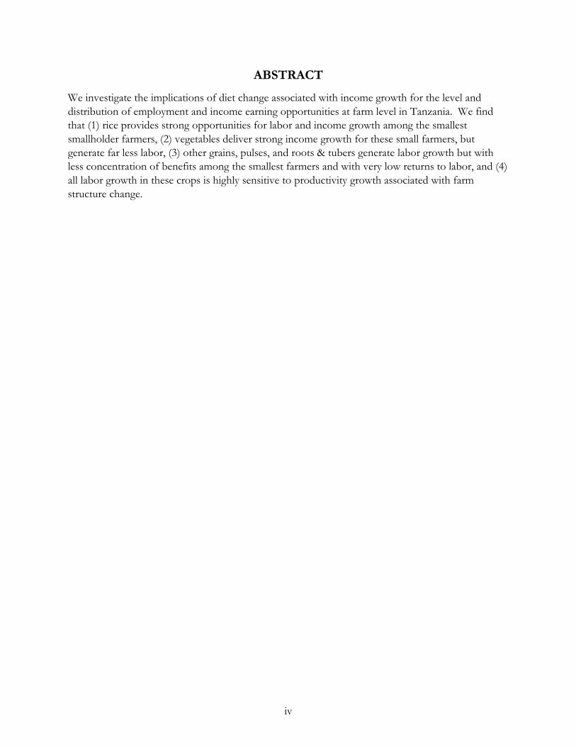
We investigate the implications of diet change associated with income growth for the level and distribution of employment and income earning opportunities at farm level in Tanzania. We find that (1) rice provides strong opportunities for labor and income growth among the smallest smallholder farmers, (2) vegetables deliver strong income growth for these small farmers, but generate far less labor, (3) other grains, pulses, and roots & tubers generate labor growth but with less concentration of benefits among the smallest farmers and with very low returns to labor, and (4) all labor growth in these crops is highly sensitive to productivity growth associated with farm structure change.

v
TABLE OF CONTENTS
Abstract .............................................................................................................................................................. iv
Table of Contents .............................................................................................................................................. v
List of Tables ..................................................................................................................................................... vi
List of Figures .................................................................................................................................................... vi
Acronyms .......................................................................................................................................................... vii
1. Introduction.................................................................................................................................................... 1
2. Data and Methods ......................................................................................................................................... 2 2.1. Data .......................................................................................................................................................... 2 2.2. Computation of Labor Input per Crop .............................................................................................. 2 2.3. Linking Consumer Expenditure to Farm Production ...................................................................... 2 2.4. Identifying the Effect of Diet Change ................................................................................................ 5 2.5. Change in Farm Structure and Associated Labor Productivity ....................................................... 6 2.6. Other Methodological Notes ............................................................................................................... 6
3. Current Dietary Patterns and Likely Directions of Change .................................................................... 7
4. Linking Diet Change to the Distribution of Employment and Returns at Farm Level .................... 12 4.1. Current Structure of Production and Productivity ......................................................................... 12 4.2. The Impact of Diet Change ............................................................................................................... 14 4.3. The Impact of Change in Farm Structure and Associated Labor Productivity .......................... 17
5. Conclusions .................................................................................................................................................. 19
Annex A. Procedure for Derivation of Labor for Crops on Fields with Multiple Crops ..................... 21 A.1. Summary for Coding in Stata ............................................................................................................ 21 A.2. Derivations and Numerical Example (See Accompanying Excel File to Show That the Numerical Example Works out Properly) ............................................................................................... 21
Annex B. Methods to Convert Consumer Food Expenditure from LSMS Expenditure Modules into Labor and Value of Production across Farming Activities ....................................................................... 23
References ......................................................................................................................................................... 26
vi
LIST OF TABLES
TABLE PAGE 1. Urban Food Budget Shares by Commodity Category and Source/Perishability/Processing
Category, Tanzania ....................................................................................................................................... 8 2. Food Budget Shares By Commodity Category and Source/Perishability/Processing Category,
Rural Tanzania ............................................................................................................................................... 9 3. Expenditure Elasticities by Various Food Characteristics, Tanzania ................................................... 10 4. Comparison Of Farm Production Value And Labor Estimates From Two Methods ..................... 13 5. Patterns of Production and Labor Productivity across Crops and Land Holding Classes,
Tanzania ....................................................................................................................................................... 13 6. The Impact of Income Growth with Diet Change: Distribution of Change in Demand and
Associated Labor, Gross Returns, and Returns per Grower ............................................................... 15 7. The Pure Impact of Diet Change: Change in Total Demand, Farm Labor, and Income per
Grower with Diet Change minus Changes without Diet Change ....................................................... 16 8. Effect of Diet Change on Total Demand for Other Crop and Livestock Activities ........................ 18 9. Impact of Structural Change in Land Holdings on Changes in Labor Due To Income Growth
with Diet Change ........................................................................................................................................ 18 B1. Parameters for Calculations of Farm Share of Consumer Expenditure ........................................... 23 B2. Resulting Factors by Source X Perishability X Processing Categories ............................................. 23
LIST OF FIGURES
B1. View of Spreadsheet Deriving Farm Labor and Production from Consumer Expenditure (Parts 1 and 2) ............................................................................................................................................................ 24 and 25

vii
ACRONYMS
AFRE Department of Agricultural, Food, and Resource Economics FAFH food away from home FSG Food Security Group FSP Food Security Policy ha hectare IFPRI International Food Policy Research Institute LQi labor:output ratios LSMS-ISA Integrated Surveys on Agriculture MSU Michigan State University NBER National Bureau of Economic Research. NPS National Panel Survey UP University of Pretoria USAID United States Agency for International Development

1
1. INTRODUCTION
The rapid growth in per capita incomes in many African countries over the past 15 years is now widely acknowledged (World Bank 2014; Radelet 2010; Young 2012), and a growing body of literature is attempting to assess its quality, sustainability, and implications. Growth in employment might be expected to be a major positive outcome of the region’s economic growth. Yet employment remains a major and growing concern, rooted in the continent’s youth bulge, in the predominance of informal self-employment in service (i.e., not manufacturing) sectors, and in the lack of any obvious evidence that this employment pattern is changing. The fear is that poor farmers leaving rural areas will have little option but to enter this vast informal sector, for returns to labor that may not be much higher than those they were earning in farming (McCullough 2015).
One impact of this economic growth is a rapidly unfolding diet transformation across the continent. Driven by Bennett’s Law, economic growth combined with rapid urbanization is driving dramatic increases in total demand for food through markets, along with a pronounced shift towards processed and perishable foods.
Yet despite its potential importance, only one study has explicitly linked changes in the level and mix of food demand to likely changes in employment. Tschirley et al. (2015a) focused on the impacts of diet change on the agrifood system of East and Southern Africa, and unbundled the post-farm portion of the system into three segments (marketing and transport, food processing, and food preparation away from home). That study left farming as a single segment. This paper will apply broadly similar methods as Tschirley et al. (2015a) to unbundle the farming sector. Given the uncertainty surrounding so many drivers of change, the paper will not attempt to project where farm labor will be located in 10 or 20 years as a result of diet change. Instead, focusing on Tanzania, it asks four questions regarding diet change as it relates to farming. First, what is the current pattern of consumption across various dimensions of food characteristics? We focus especially on food’s commodity content, perishability, level of processing, and mode of access (markets or own production).
Second, how is food demand likely to change in coming years across these dimensions?; which types of foods will see the most rapid rate of growth?; which are contributing most to absolute growth in demand? Third, what opportunities for employment generation and income enhancement does this change create at farm level? The opportunities we focus on are for employment generation and income enhancement.
Fourth, how are these opportunities distributed across farmers? We employ a total land holding classification, and its structure across producers of different commodities, to examine this distribution.
The paper is organized as follows. Section two summarizes data and methods. Section three focuses on our first two questions: the current pattern of consumption and its likely change over time. Section four addresses our third and fourth questions, regarding the distribution of opportunities across types of farmers. Section five concludes.
2
2. DATA AND METHODS
2.1. Data
Data for this analysis come from two sources. First, the agricultural module of Tanzania’s 2010/11 National Panel Survey (NPS) was used to compute, at plot level, the labor input, quantity, and value of production, and area devoted to all available crops. The NPS is one of the LSMS-ISA (Integrated Surveys on Agriculture) surveys that collected by national statistical agencies with assistance from World Bank and other organizations, and which provide much greater detail on agricultural practices than previous LSMS surveys. The work in this paper could not be done without this kind of detailed data. Data from sections 2, 3, 4, 5, and 11 of the agricultural questionnaire were used for these purposes. Section B (demographics) of the household survey was also used.
Second, Comtrade data were used at the four- and six-digit level to establish import values for each of the food categories we use in this paper. Six-digit figures were used only when four-digit descriptions were insufficient to allow clear classification of an item into our categorization scheme.
2.2. Computation of Labor Input per Crop
A key element in the analysis is the computation of labor input for crops at household level. Together with the value of production, this labor input is used to compute labor: output ratios for each crop (LQi), which are the key factor allowing the linking of consumer demand to farm labor. A methodological complication arises due to the fact that labor was collected for each plot, not for each crop on each plot. For plots with more than one crop, allocating the plot’s labor to each crop is not straightforward. Yet only 59% of all fields in the NPS had only one crop; limiting the computations to those fields would have nearly halved the amount of data with which to work. We therefore used the methods described in Annex A to impute labor on all crops with fields holding up to three crops; this covered 98% of all fields in the database. Briefly, the method takes advantage of relative LQ ratios across crops on fields with only one crop, together with information on the area share of each crop on multi-cropped fields, to estimate labor for each of the crops on those fields.
2.3. Linking Consumer Expenditure to Farm Production
We link consumer expenditure to farm production using methods adapted from Tschirley et al. (2015a). Two challenges emerge in making this link. First, the rise of processed foods and of food away from home (FAFH) means that many food products purchased by consumers have multiple ingredients. Linking to farm production requires plausible estimation of the shares of specific farm commodities in these food products. We did this based on a wide online search of recipes for items such as bread and other bakery products, breakfast porridges, manufactured drinks, and others.1
The second challenge is that the farm value of final consumer expenditure depends on the level of processing that the item(s) has undergone. We estimate that in Tanzania, 41% of all consumer expenditure on wheat, rice, other grains, pulses, and roots and tubers is in the form of processed foods; 33% of this is on foods with relatively low value-added processing, and 8% on foods with high value added. Another 21% of expenditure on these commodities comes in the form of FAFH, which has additional value added after the farm. Thus, over 60% of farm commodity consumption 1 Specific recipes used for each item are available on request.
3
in Tanzania undergoes varying degrees of post-farm transformation that add costs beyond basic marketing and transport. Perishable commodities can also be expected to have higher post-farm costs, due either to cold chain maintenance or higher losses due to perishability. Imputation of farm value from consumer expenditure values must account for these factors.
To do so, we classify consumer food expenditure into a matrix defined by two vectors: one based on source (purchased or own production), perishability (perishable or not), and level of processing (high, low, and not processed); and another based on commodity. We then apply differing farm value share coefficients based on the first vector.2
Specific methods for this paper proceed in two broad steps. First, we convert the value consumer food expenditure as given in original expenditure items in LSMS expenditure modules into the value of demand for agricultural commodities at farm gate, net of imports. We do this as follows:
1. Categorize all food expenditure items (e) from the LSMS data set into nine food expenditure categories (f) based on source of supply (consumed own production or purchased), processing level, and perishability.
2. Compute household expenditure on each food item e in each of the nine food expenditure categories f (𝑉𝑉𝑒𝑒𝑒𝑒ℎ )
3. Define 12 commodity groups 4. Convert household expenditure on each food item e in each food category f into expenditure
on each commodity group i in each food category f as follows: a. Note that processed food expenditure items may have multiple commodities as
ingredients; b. Map single ingredient expenditure items e in each food category f directly into the 12
commodity groups i; c. Map multiple ingredient expenditure items e in each food category f into the 12
commodity groups i as follows:
𝑉𝑉𝑉𝑉𝑖𝑖𝑒𝑒𝑒𝑒 =𝑃𝑃𝑖𝑖𝑖𝑖𝑄𝑄𝑄𝑄𝑖𝑖𝑖𝑖𝑖𝑖∑ 𝑃𝑃𝑖𝑖𝑖𝑖𝑄𝑄𝑄𝑄𝑖𝑖𝑖𝑖𝑖𝑖𝑖𝑖
(1)
𝑉𝑉𝑖𝑖𝑒𝑒𝑒𝑒ℎ = 𝑉𝑉𝑉𝑉𝑖𝑖𝑒𝑒𝑒𝑒𝑉𝑉𝑒𝑒𝑒𝑒ℎ (2)
𝑉𝑉𝑖𝑖𝑒𝑒ℎ = ∑ 𝑉𝑉𝑖𝑖𝑒𝑒𝑒𝑒ℎ𝑒𝑒 (3)
Where,
i. e = food expenditure item from survey data; ii. i = commodity group as defined in step 2; iii. Pif = consumer price of commodity group i in food group f (computed as
medians at defined geographical levels from survey data);
2 Parameters can be found in Annex A. Sensitivity analysis shows that changes of up to 20 percentage points in these parameters results in changes of less than one-half a percentage point in final results on the effect of diet change on labor. Changed parameters do have more substantial effects on the match between farm labor computed directly from the agricultural modules of NPS and farm labor estimated from consumer demand using the methods outlined here. Yet the results of interest—impacts of diet change on labor and its distribution across crops and farms—change in no meaningful way.

4
iv. 𝑄𝑄𝑉𝑉𝑖𝑖𝑒𝑒𝑒𝑒 = quantity share of each commodity group i in food expenditure item e within food category f;3
v. 𝑉𝑉𝑒𝑒𝑒𝑒ℎ = expenditure value (from survey data) on food expenditure item e in food category f for household h;
vi. VSief = value share of commodity group i as an ingredient in food expenditure item e within food category f;
vii. 𝑉𝑉𝑖𝑖𝑒𝑒𝑒𝑒ℎ = value of expenditure by household h on ingredient i in food expenditure item e within each food category f;
viii. 𝑉𝑉𝑖𝑖𝑒𝑒ℎ = total expenditure value by household h, across all food expenditure items e, on commodity ingredient i within each food category f;
d. Sum across all households to compute total market expenditure at consumer level on each commodity group i within each food category f:
𝑉𝑉𝑖𝑖𝑒𝑒 = ∑ 𝑉𝑉𝑖𝑖𝑒𝑒ℎℎ (4)
5. Convert total market expenditure (consumer level) on commodity group i within each food expenditure category f (𝑉𝑉𝑖𝑖𝑒𝑒) into the value at farm-level of demand for each i in f (𝑉𝑉𝑖𝑖𝑒𝑒′ ), taking into account the import share of each food category f:
𝑉𝑉𝑖𝑖𝑒𝑒′ = 𝑉𝑉𝑖𝑖𝑒𝑒𝐶𝐶𝑒𝑒�1 − 𝐼𝐼𝑒𝑒� (5)
Where,
i. Cf = share of consumer value accruing to the farmer, by perishability, level of processing, and source of supply, developed from secondary data;
ii. 𝑉𝑉𝑖𝑖𝑒𝑒′ = value at farm-level of demand for each i in f, and iii. 𝐼𝐼𝑒𝑒 = the import share for food category f
6. Compute total value of demand at farm level for each i: 𝑉𝑉𝑖𝑖′ = ∑ 𝑉𝑉𝑖𝑖𝑒𝑒′𝑒𝑒 (6)
Second, we convert the farm-gate value of demand for farm commodities into labor demand on the farm to produce those commodities. We achieve this through the following steps:
7. Compute production-weighted farm labor:output ratios for each commodity ingredient group i:
𝐿𝐿𝑄𝑄𝑖𝑖 = ∑ 𝐿𝐿𝑖𝑖ℎ′
ℎ∑ 𝑉𝑉𝑖𝑖ℎ
′ℎ
� (7)
Where i. 𝑉𝑉𝑖𝑖ℎ
′= household value of production of commodity group i computed from
LSMS-ISA data, and ii. 𝐿𝐿𝑖𝑖ℎ
′= days of farm labor (family and hired) the household used to produce i,
8. Convert farm-level value of demand for each commodity group i into farm labor to produce
i:
3 𝑄𝑄𝑉𝑉𝑖𝑖𝑒𝑒 = 1 for single ingredient items. For multiple ingredient items, 𝑄𝑄𝑉𝑉𝑖𝑖𝑒𝑒 is obtained from secondary information on recipes (see Annex X for data sources on these recipes)

5
𝐿𝐿𝑖𝑖′ = 𝑉𝑉𝑖𝑖′𝐿𝐿𝑄𝑄𝑖𝑖 (8)
9. Note that LQi can be computed for other levels by altering the summation function in (7). For example, LQ can be computed for production of each crop i within farm size categories by computing (7) at that level.
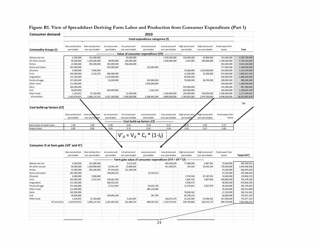
Figure B1 shows a graphic of the implementation of these methods. The source x perishability x processing vector generally follows Tschirley et al. (2015a), with categories for consumed own production, unprocessed purchased food, and purchased processed food with low- and high value added. Each of these is further broken into perishable and non-perishable. Together with a separate category for FAFH, this procedure generates nine source x perishability x processing categories.
Purchased foods are unprocessed if they undergo no transformation from their original state beyond removal from the plant and (for non-perishables) drying. Processed foods are assigned to the high-value added category if they satisfy at least two of the following three conditions: multiple ingredients; physical change induced by heating, freezing, extrusion, or chemical processes (i.e., more than simple physical transformation); and packaging more complex than simple paper or plastic. Foods satisfying one of those criteria are classified as low-value added processed.
Twelve commodity categories are used in the second vector: wheat and rice, all other cereals, pulses, roots and tubers, vegetable oils, fruit, vegetables, poultry and eggs, other meat, dairy, fish, and other food. Of the resulting 108 cells of the matrix, 63 contain positive expenditure in Tanzania. The structure of the classification and the cells that have positive expenditure data can be seen in Table 1 of the next section, and in Figure B1.
The Tanzania NPS (and other ISA surveys) do not collect detailed labor data on livestock activities or on tree crops. As a result, dairy, poultry, other livestock, and fruit trees could not be included in the farm level of this analysis. Thus, while we characterize the diet transformation across all elements in the two classification vectors, the implications for farm employment are discussed only for six commodity categories: wheat and rice, other grains, pulses, roots and tubers, oilseeds, and vegetables. We include a non-food cash crop category, dominated by cotton and tobacco, for comparison with patterns among food crops.
2.4. Identifying the Effect of Diet Change
We identify the effect of diet change in two ways: (1) by comparing a scenario of income growth combined with its associated diet change to the baseline, and (2) by comparing these results to those from a scenario of income growth without diet change. No diet change is defined as no change in food budget shares as a result of income growth. In this second approach, the expenditure elasticity of demand for all food is assumed to remain constant between the two scenarios, so that total food expenditure at the end of the projection period is the same between the two scenarios. This second approach amounts to a thought experiment to identify the pure effect of diet change, and serves to highlight the over-riding role that Engel’s Law has in determining the farm labor impacts of income growth.

6
2.5. Change in Farm Structure and Associated Labor Productivity
To examine how robust the labor results are, we develop one scenario on changes in farm structure and associated labor productivity and examine its impacts on the change in labor associated with combined income growth and diet change (our first approach to identifying the effects of diet change).
2.6. Other Methodological Notes
Our projection period is short: one year. The motivation for this approach is to focus not on the unanswerable question of how all labor will be distributed within the farm sector 10 or 20 years hence, but on the more answerable question of where within the farm sector—for what crops and which farmers—diet change may be increasing or decreasing opportunities, and by how much. Because labor intensity can differ widely across activities and across farmers within those activities, it is not obvious how even a well-understood change in the mix of foods demanded by consumers will affect the distribution of labor across the farming activities that produce them.
The projection ignores population change because growth is modeled in per capita terms, so total population change has no impact on results. Changes in the share of population in rural and urban areas would affect results, but over our short time frame, this does not come into play.
The projection nets out imports by comparing the mean value of imports from Comtrade for each cell in the matrix of Table 1 to consumer expenditure; values are then aggregated into the source x perishability x processing categories and demand at farm level is reduced proportionally4. The exercise also assumes that import shares will remain constant. Thus, rising (falling) import shares will push down (up) estimates of labor and income growth.
Results from the exercise should be interpreted as the distribution of short-run opportunities at farm level engendered by diet change alone, before prices change, investments take place, and the structure of land holdings and productivity can change in response to these opportunities.
4 Import shares were 1% for unprocessed perishable and low processed perishable; 70% for unprocessed non-perishable (driven almost entirely by wheat); 4% for low processed non-perishable (e.g., rice), 2% for high processed perishable (e.g., dairy), and 57% for high processed non-perishable. The latter category is driven almost entirely by imports of vegetable oil.

7
3. CURRENT DIETARY PATTERNS AND LIKELY DIRECTIONS OF CHANGE
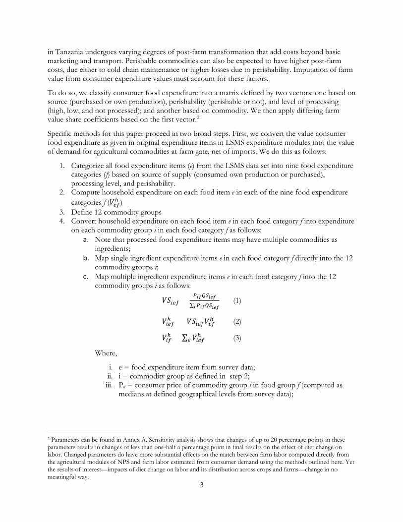
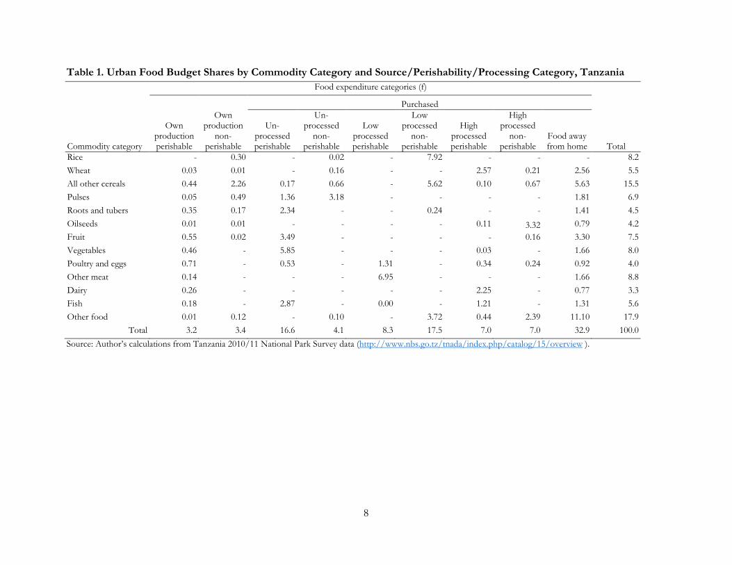
We first review current patterns of consumption in urban and rural areas by examining food budget shares by the matrix of commodity by source x perishability x processing categories (Tables 1 and 2). Five patterns stand out. First, purchased foods dominate consumption in both rural and urban areas; in rural areas, purchased food accounts for more than half (56%) of the value of all food consumption5. Consumption commercialization has proceeded very far in rural Tanzania.
Second, the share of processed food (including FAFH) in consumption is high in both urban and rural areas. In urban areas, processed foods and FAFH occupy 73% of all expenditures on food (purchased plus own production), and 78% of all food purchases. Shares in rural areas are 42% and 74%. Thus, as a share of purchased food, processed food and FAFH are nearly as high in rural areas as they are in urban, and occupy nearly half of all rural expenditures even when including consumed own production.
Third, most processed food consumption is of highly processed foods and FAFH, rather than low processed foods. In rural areas, highly processed and FAFH account for 39% of all purchases and 53% of processed food purchases; the shares in urban areas are 50% and 65%.
Fourth, these high shares of processed food consumption matter to our analysis, because large shares of grains, pulses, and roots and tubers are obtained in processed form. In urban areas, 71% of these basic foods are obtained already processed, while in rural areas 33% are obtained in this way. Of the purchased grains, pulses, and roots and tubers in rural areas, 74% are obtained in processed form. Once again, there is little to distinguish urban and rural households with regard to their behavior as consumers in food markets.
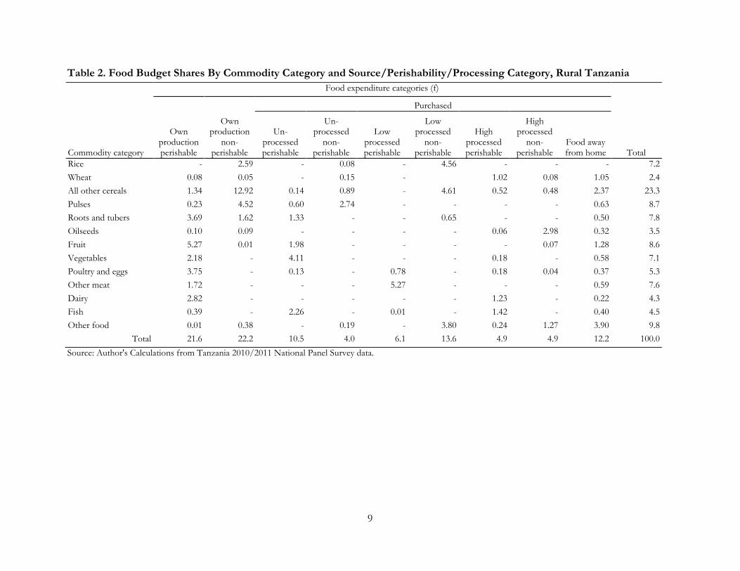
The elasticities in Table 3 suggest how these consumption patterns will change as incomes rise. We categorize the food in various ways in this table to allow a richer discussion. Several patterns stand out. First, elasticities for purchased food are near unitary in both rural and urban areas; in rural areas, they rise above 1.0 in the middle-income tercile and remain there in the top tercile, while in urban they fall steadily but high, 0.70, in the top tercile. Elasticities on own production, on the other hand, fall dramatically across income terciles in rural areas, and are uniformly negative in urban areas. Thus, the process of consumption commercialization, noted elsewhere as well (Dolislager forthcoming) is well established in Tanzania.
Second, demand elasticities for processed foods exceed those for unprocessed, though not by a huge margin. Third, the difference between perishable and non-perishable is far larger, at 1.11 vs. 0.61 in rural areas and 0.70 vs. 0.46 in urban areas. Elasticities for non-perishable foods (which include the great majority of basic staple consumption) fall to 0.27 within the top income tercile in urban areas.
Fourth, food away from home has the highest or near highest elasticity in every tercile in both rural and urban areas; note also from Tables 1 and 2 that budget shares for FAFH are substantial in rural areas, at 12.2% and nearly triple that, at 33%, in urban areas. This combination of high budget shares and high elasticities suggests that FAFH will be a major area of growth throughout Tanzania’s food system for the foreseeable future. This pattern is well established by now across east and southern Africa (Dolislager forthcoming) and other countries (Seto and Ramankutty 2016).
5 Note that, at consumer level, consumed own production is valued with the same prices applied to purchased food. Differing prices thus do not drive this result.
8
Table 1. Urban Food Budget Shares by Commodity Category and Source/Perishability/Processing Category, Tanzania Food expenditure categories (f)
Purchased
Commodity category
Own production perishable
Own production
non-perishable
Un-processed perishable
Un-processed
non-perishable
Low processed perishable
Low processed
non-perishable
High processed perishable
High processed
non-perishable
Food away from home Total
Rice - 0.30 - 0.02 - 7.92 - - - 8.2 Wheat 0.03 0.01 - 0.16 - - 2.57 0.21 2.56 5.5 All other cereals 0.44 2.26 0.17 0.66 - 5.62 0.10 0.67 5.63 15.5 Pulses 0.05 0.49 1.36 3.18 - - - - 1.81 6.9 Roots and tubers 0.35 0.17 2.34 - - 0.24 - - 1.41 4.5 Oilseeds 0.01 0.01 - - - - 0.11 3.32 0.79 4.2 Fruit 0.55 0.02 3.49 - - - - 0.16 3.30 7.5 Vegetables 0.46 - 5.85 - - - 0.03 - 1.66 8.0 Poultry and eggs 0.71 - 0.53 - 1.31 - 0.34 0.24 0.92 4.0 Other meat 0.14 - - - 6.95 - - - 1.66 8.8 Dairy 0.26 - - - - - 2.25 - 0.77 3.3 Fish 0.18 - 2.87 - 0.00 - 1.21 - 1.31 5.6 Other food 0.01 0.12 - 0.10 - 3.72 0.44 2.39 11.10 17.9
Total 3.2 3.4 16.6 4.1 8.3 17.5 7.0 7.0 32.9 100.0 Source: Author’s calculations from Tanzania 2010/11 National Park Survey data (http://www.nbs.go.tz/tnada/index.php/catalog/15/overview ).
9
Table 2. Food Budget Shares By Commodity Category and Source/Perishability/Processing Category, Rural Tanzania Food expenditure categories (f)
Purchased
Commodity category
Own production perishable
Own production
non-perishable
Un-processed perishable
Un-processed
non-perishable
Low processed perishable
Low processed
non-perishable
High processed perishable
High processed
non-perishable
Food away from home Total
Rice - 2.59 - 0.08 - 4.56 - - - 7.2 Wheat 0.08 0.05 - 0.15 - 1.02 0.08 1.05 2.4 All other cereals 1.34 12.92 0.14 0.89 - 4.61 0.52 0.48 2.37 23.3 Pulses 0.23 4.52 0.60 2.74 - - - - 0.63 8.7 Roots and tubers 3.69 1.62 1.33 - - 0.65 - - 0.50 7.8 Oilseeds 0.10 0.09 - - - - 0.06 2.98 0.32 3.5 Fruit 5.27 0.01 1.98 - - - - 0.07 1.28 8.6 Vegetables 2.18 - 4.11 - - - 0.18 - 0.58 7.1 Poultry and eggs 3.75 - 0.13 - 0.78 - 0.18 0.04 0.37 5.3 Other meat 1.72 - - - 5.27 - - - 0.59 7.6 Dairy 2.82 - - - - - 1.23 - 0.22 4.3 Fish 0.39 - 2.26 - 0.01 - 1.42 - 0.40 4.5 Other food 0.01 0.38 - 0.19 - 3.80 0.24 1.27 3.90 9.8
Total 21.6 22.2 10.5 4.0 6.1 13.6 4.9 4.9 12.2 100.0 Source: Author's Calculations from Tanzania 2010/2011 National Panel Survey data.
10
Table 3. Expenditure Elasticities by Various Food Characteristics, Tanzania
Rural Terciles Urban Terciles
Characteristic Bottom tercile
Middle tercile Top Overall
Bottom tercile
Middle tercile Top Overall
Food source Purchased 0.76 1.11 1.09 0.98 1.12 0.99 0.70 0.94 Own production 1.29 0.75 0.33 0.79 -0.14 -1.36 -0.56 -0.69
Processing content All processed 0.70 1.01 0.96 0.89 1.04 0.89 0.48 0.81 All unprocessed 0.57 0.86 1.10 0.84 0.92 0.61 0.43 0.65
Perishability Perishable 1.04 1.40 0.89 1.11 0.91 0.64 0.54 0.70 Non-perishable 0.96 0.35 0.51 0.61 0.67 0.45 0.27 0.46
Source x Processing x Perishability Food away from home (FAFH) 1.53 1.92 1.35 1.44 1.93 1.50 1.04 1.28 Low processed perishable 1.53 2.01 1.09 1.29 1.74 1.23 0.66 1.04 High processed non-perishable 1.25 1.37 1.27 1.17 1.28 1.07 0.85 0.91 High processed perishable 0.91 0.44 0.87 1.01 1.31 1.15 0.60 0.83 Own production perishable 1.14 1.68 0.66 1.00 -0.05 -1.66 -0.67 -0.27 Un-processed perishable 0.76 0.90 1.15 0.94 0.88 0.74 0.54 0.81 Low processed non-perishable 0.33 0.69 0.77 0.78 0.72 0.63 0.10 0.54 Un-processed non-perishable 0.23 0.77 0.93 0.55 1.02 0.16 -0.13 0.34 Own production non-perishable 1.37 -0.01 -0.10 0.44 -0.21 -1.06 -0.45 -0.60
Commodity Wheat 1.85 2.82 1.29 1.45 1.55 1.23 0.78 1.22 Fruit 1.59 1.90 0.95 1.32 1.12 0.14 0.91 1.07 Other meat 1.92 2.39 1.19 1.31 1.66 1.37 0.73 1.04 Poultry and eggs 1.35 1.84 1.02 1.27 1.54 1.45 0.66 1.03 Other food 1.29 1.41 1.11 1.26 1.25 1.41 0.88 1.06 Rice 1.87 1.46 0.83 1.11 1.51 0.71 0.19 0.93 Dairy 1.93 1.81 0.79 1.11 1.60 1.98 0.87 0.94 Oils and oilseeds 1.33 0.75 0.85 0.95 0.88 0.61 0.51 0.78 Fish 0.84 0.90 1.08 0.93 0.58 0.50 0.51 0.79 Pulses 1.46 0.34 0.62 0.78 0.66 0.62 0.41 0.70 Vegetables 0.34 0.08 0.66 0.62 0.43 0.49 0.60 0.77 All other grains 0.89 -0.05 0.30 0.48 0.39 0.13 0.61 0.47 Roots and tubers 0.11 1.19 0.69 0.46 0.39 0.87 0.62 0.61
Source: authors' calculations from Tanzania 2010/11 National Panel Survey data.
Fifth, elasticities for consumed own production of non-perishable foods–mostly maize and other grains, and pulses, collapse across income terciles in rural areas, from 1.37 in the poorest group to -0.10 in the least poor. This implies that the poorest rural farmers consume large portions of their incremental staple food production, but move rapidly towards market purchases as incomes rise.
Sixth, a number of points arise when focusing on commodities (the bottom portion of Table 3). Wheat has the highest elasticity in both rural and urban areas, reaching a remarkable 1.45 in the former. In both areas, fruit is next, each with elasticities above unity. After this come meat, poultry and eggs, and rice and dairy, lying between 1.3 and 1.1 in rural areas and between 1.04 and 0.93 in urban areas. Note, however, that the elasticity for rice falls far more dramatically across income
11
terciles than that of any other commodity: from 1.87 to 0.83 in rural areas and from 1.51 to 0.19 in urban areas. In fact, rice has by far the lowest elasticity of demand of any commodity within the third (wealthiest) tercile of urban areas.
Notably, vegetables have the third lowest elasticity in rural areas and the fourth lowest in urban areas. This will stand as a surprise to many, as horticulture is broadly seen as an important source of growth for small farmers as economies urbanize and incomes rise. One possibility is that the data collection methods used in the expenditure module of NPS fail to capture new and minor products whose demand could grow rapidly as incomes rise. Vegetables could be especially subject to this bias, given the large number of different types that exist. Further research is needed on this topic, given the discrepancy between elasticities reported here and common perceptions about these foods.6
6 Note that Gibson et al. (2015) cite Pradhan in noting that “survey reporting tasks become harder for richer household with more varied consumption.” Note also that elasticity estimates on vegetables from other countries deliver very similar results to those reported here for Tanzania.

12
4. LINKING DIET CHANGE TO THE DISTRIBUTION OF EMPLOYMENT AND RETURNS AT FARM LEVEL
4.1. Current Structure of Production and Productivity
We start this section by comparing the values of farm production from two different methods: values implied by the NPS consumer expenditure data, our farm share factors, and import shares; and that computed directly from the farm production modules of NPS. Relatedly, we compare the farm labor implied by consumer demand (estimated as in Annex B) to that computed directly from the NPS farm labor and production modules (Table 4).
Values are remarkably close except for roots and tubers, and vegetables. For roots and tubers, the reason is clear: NPS did not include cassava in the plot registry but rather in the permanent crops section, and thus did not collected detailed labor data for it. We therefore were unable to include the value of this crop in our calculations. To adjust for this, we used data from Uganda, which did collect labor on cassava: we set cassava’s LQ ratio in TZ by calculating the ratio of cassava’s LQ ratio to the mean of other crops’ LQ ratio in Uganda.
For vegetables, note that farm data generate nearly the exact same proportional difference, compared to results derived from consumed expenditure data, for both labor and production value. We suggest that the discrepancy is due to the extreme difficulty of collecting accurate production and labor data for vegetables in a single visit survey.7 This difficulty stems from the fact that many vegetables are harvested repeatedly over the course of the year, some as frequently as every four weeks, during the wet season and, for those with irrigation, the dry season. Accurately recalling production and labor over the course of a full year is nearly impossible, with the resulting estimates highly likely to be biased downwards. Because labor and production value show nearly identical discrepancies between the two methods, we used LQ values for vegetables as calculated from the farm data, and applied it to the value of production derived from consumer expenditure, resulting in much higher estimates of labor than from the farm module.
With these adjustments, Table 5 shows the share of production and labor productivity (captured by LQ ratios8) across five farm size categories based on total land holdings: less than 1 hectare, 1-2 hectare (ha), 2-5 ha, 5-10 ha, and > 10 ha.
Four patterns stand out. First, production of roots and tubers and of vegetables is most concentrated among the smallest farmers. This is not surprising for vegetables, but may be for roots and tubers. Second, oilseeds are the least produced by the smallest farmers, who have only an 8% production share in this crop. Among the largest land holders, vegetables and oilseeds are nearly absent: the NPS sample held only three farmers with oilseeds and one with vegetables in that largest land holding class.
Third, labor productivity, as reflected by the inverse of the LQ ratios, is lowest among the smallest farmers in every crop. In most crop groups, labor productivity rises (LQ ratios fall) consistently into the second-largest class (5-10 ha) before typically rising in the largest land holding class. The limited number of observations in this largest class suggests that not too much should be drawn from this latter pattern.
7 See Arthi et al. (2013) for a discussion of methodological problems in the collection of household farm labor data. 8 All LQ ratios used in this paper are computed as production-weighted means of household LQ ratios, at whatever level they are reported.

13
Table 4. Comparison of Farm Production Value and Labor Estimates from Two Methods Computed from Farm Production
and Labor Modules Derived from Consumer
Expenditure Modules Ratio Value of
Production Days of Labor Value of
Production Days of Labor Value of
Production Days of Labor
Wheat and rice 900,272,534 137,139,581 900,560,013 137,183,373 1.00 1.00 All other cereals 1,923,428,030 526,132,136 1,946,468,588 532,434,622 0.99 0.99 Pulses 627,244,617 195,108,687 666,879,839 207,437,491 0.94 0.94 Roots and tubers 164,166,476 82,097,968 587,080,646 165,534,953 0.28 0.50 Oilseeds 126,992,211 19,123,745 129,856,570 19,555,088 0.98 0.98 Vegetables 160,169,076 12,483,007 674,892,509 52,598,717 0.24 0.24
Source: Author's Calculations from Tanzania 2010/2011 National Panel Survey. Table 5. Patterns of Production and Labor Productivity across Crops and Land Holding Classes, Tanzania
Total land holding size class Overall < 1 ha 1-2 ha 2-5 ha 5-10 ha > 10 ha
Current shares of production Wheat and Rice 0.26 0.25 0.29 0.11 0.09 1.00 Other Grains 0.21 0.27 0.30 0.18 0.04 1.00 Pulses 0.21 0.28 0.31 0.11 0.09 1.00 Oilseeds 0.08 0.24 0.29 0.38 1.00 Roots and Tubers 0.34 0.34 0.25 0.05 0.03 1.00 Vegetables 0.28 0.33 0.34 0.04 1.00 Other cash crops (mostly cotton and tobacco)
0.10 0.20 0.43 0.18 0.09 1.00
Current LQ (days labor per USD output)
Wheat and Rice 0.18 0.15 0.14 0.06 0.08 0.14 Other Grains 0.35 0.31 0.28 0.12 0.31 0.28 Pulses 0.44 0.35 0.28 0.17 0.21 0.32 Oilseeds 0.29 0.22 0.16 0.07 0.15 Roots and Tubers 0.39 0.20 0.29 0.25 0.40 0.30 Vegetables 0.11 0.08 0.08 0.13 0.09
Source: Authors' calculations from Tanzania 2010/11 National Park Survey data. Note: Output in LQ ratios is in value terms and ratios are production-weighted within each farm size class. Values deleted from top land class in oilseeds and vegetables because based only 3 observations and 1 observation, respectively.
Vegetables are a partial exception to this pattern: though productivity is lowest in the smallest land holding class, it reaches its maximum between 1 and 5 hectares, and rises in the 5-10 ha class.
Fourth, vegetables have by far the lowest LQ ratios (highest labor productivity) of any food crop, being only slightly more than half the level of rice in the first three land classes. This suggests that even rapid growth in the demand for vegetables, while fueling remunerative opportunities for small farmers able to produce for the market, will not do so for large numbers of farmers.
14
Finally, rice shows by far the lowest LQ ratios among grains and pulses, and is lower even than vegetables in the fourth class (5-10 ha). Thus, among the grains, rice may present positive opportunities for remunerative farming, but for more modest numbers of households than other grains.
4.2. The Impact of Diet Change
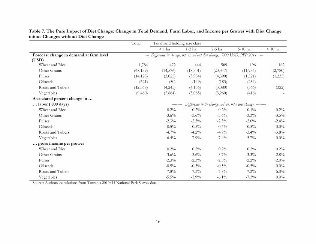
Tables 6 and 7 implement our two approaches to identifying the impact of diet change across crops and land holding classes. Table 6 links the structure of farm production and labor productivity shown in Table 5 to demand projections under income growth with diet change, as explained in the methods section. Table 7 summarizes, in the same structure, the difference in change between scenarios of income growth with and without diet change; negative values indicate a negative pure effect of diet change.
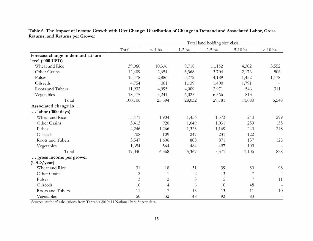
Several results stand out when examining Table 6 First, rice9 generates the highest absolute growth in demand and labor of any category at farm level, nearly double the next group, and delivers the second highest incremental income per grower.
Second, vegetables stand second in total demand, only fifth in labor (due to their low LQ ratios) but generate the highest incremental returns per grower in every land size category. Note also that new demand for vegetables is heavily concentrated among farms under 5 ha. Vegetables present major opportunities for income growth among a reduced set of small farmers.
Third, pulses and other grains both generate strong growth in labor but very low incremental income to growers.
Three types of crops emerge from this analysis: (1) rice, with high growth in demand and labor and strong returns to farmers, all a result of a substantial base of demand and continuing high elasticities of demand in rural areas and among the bottom two-thirds of consumer in urban areas; (2) vegetables, with strong growth and high incremental returns to growers, but with very modest labor impact; and (3) other grains, pulses, and roots and tubers, all with strong bases of demand, substantial labor creation, but very low returns to growers.
Table 7 captures the pure effect of diet change. The outstanding result from this analysis is that pure diet change has a positive effect on labor and associated indicators only for rice (this was fully predictable from the fact that it was the only crop in this group with an elasticity of demand above 1.0), but that the gains it delivers are tiny—well below a 1% increase in the amount of labor that these farmers were employing and the gross income they were generating.
This latter finding holds true also for the crop and livestock activities for which the NPS does not collect detailed labor data and which for that reason have been excluded from this analysis.
9 At farm level, over 99% of the wheat and rice category is rice.
15
Table 6. The Impact of Income Growth with Diet Change: Distribution of Change in Demand and Associated Labor, Gross Returns, and Returns per Grower
Total Total land holding size class
< 1 ha 1-2 ha 2-5 ha 5-10 ha > 10 ha Forecast change in demand at farm level (‘000 USD)
Wheat and Rice 39,060 10,336 9,718 11,152 4,302 3,552 Other Grains 12,409 2,654 3,368 3,704 2,176 506 Pulses 13,478 2,886 3,772 4,189 1,452 1,178 Oilseeds 4,754 381 1,139 1,400 1,791 - Roots and Tubers 11,932 4,095 4,009 2,971 546 311 Vegetables 18,475 5,241 6,025 6,366 813 -
Total 100,106 25,594 28,032 29,781 11,080 5,548 Associated change in … … labor ('000 days)
Wheat and Rice 5,471 1,904 1,456 1,573 240 299 Other Grains 3,413 920 1,049 1,031 259 155 Pulses 4,246 1,266 1,323 1,169 240 248 Oilseeds 708 109 247 231 122 - Roots and Tubers 3,547 1,606 808 871 137 125 Vegetables 1,654 564 484 497 109 -
Total 19,040 6,368 5,367 5,371 1,106 828 … gross income per grower (USD/year)
Wheat and Rice 31 18 31 39 80 98 Other Grains 2 1 2 3 7 4 Pulses 3 2 3 5 7 11 Oilseeds 10 4 6 10 48 - Roots and Tubers 11 7 15 13 11 10 Vegetables 50 32 48 93 83 -
Source: Authors' calculations from Tanzania 2010/11 National Park Survey data.
16
Table 7. The Pure Impact of Diet Change: Change in Total Demand, Farm Labor, and Income per Grower with Diet Change minus Changes without Diet Change
Total Total land holding size class < 1 ha 1-2 ha 2-5 ha 5-10 ha > 10 ha
Forecast change in demand at farm level (USD)
--- Difference in change, w/ vs. w/out diet change, '000 USD, PPP 2011 ---
Wheat and Rice 1,784 472 444 509 196 162 Other Grains (68,159) (14,576) (18,501) (20,347) (11,954) (2,780) Pulses (14,125) (3,025) (3,954) (4,390) (1,521) (1,235) Oilseeds (621) (50) (149) (183) (234) - Roots and Tubers (12,368) (4,245) (4,156) (3,080) (566) (322) Vegetables (9,460) (2,684) (3,085) (3,260) (416) -
Associated percent change in … … labor ('000 days) --------- Difference in % change, w/ vs. w/o diet change ---------
Wheat and Rice 0.2% 0.2% 0.2% 0.1% 0.2% Other Grains -3.6% -3.6% -3.6% -3.3% -3.5% Pulses -2.3% -2.3% -2.3% -2.0% -2.4% Oilseeds -0.5% -0.5% -0.5% -0.5% 0.0% Roots and Tubers -4.7% -4.2% -4.7% -3.4% -3.8% Vegetables -6.4% -7.9% -7.4% -5.7% 0.0%
… gross income per grower Wheat and Rice 0.2% 0.2% 0.2% 0.2% 0.2% Other Grains -3.6% -3.6% -3.7% -3.3% -2.8% Pulses -2.3% -2.3% -2.3% -2.2% -2.0% Oilseeds -0.5% -0.5% -0.5% -0.5% 0.0% Roots and Tubers -7.8% -7.3% -7.8% -7.2% -6.0% Vegetables -5.5% -5.9% -6.1% -7.3% 0.0%
Source: Authors' calculations from Tanzania 2010/11 National Park Survey data.

17
Table 8 shows that fruit, poultry and eggs, other meat, and other food all gain from diet change, while dairy and fish lose, but that in every case the pure impacts of diet change are tiny – less than 1% of starting values.
4.3. The Impact of Change in Farm Structure and Associated Labor Productivity
We close this section by examining the sensitivity of our results in Table 6 (income growth with diet change) to changes in farm structure and associated labor productivity. Recall from section 4.a that in every crop group, LQ ratios fall steadily from the smallest to the second-largest land holding category (from <1 ha up to 5-10 ha) before rising in the largest category (>10 ha; vegetables start rising in the 5-10 ha category). In this scenario we posit that (a) 1% of the farms in each farm size category rise into the next larger category and take on the LQ values of their new category, and (b) farms in the largest land holding category take-on the (lower) labor productivity of the 5-10 ha group. This latter assumption would be an expected pattern as investment in the sector increases in response to growing markets.
This structural change in land holdings results in production weighted LQ ratios falling (labor productivity rising) for all crop groups except vegetables, by between 0.9% (for oilseeds) and 4.7% (for other grains). Labor productivity falls (LQ ratios rise) by 2.3% in vegetables due to the structure of production and productivity reflected in Table 5: labor productivity for this group reaches its maximum in the 2-5 ha category, and declines sharply in the 5-10 ha category.
Table 9 summarizes the results of these changes on labor demand: labor gains from income growth with diet change are eliminated for rice and pulses, labor falls by over 4% for other grains, and labor gains are reduced in oilseeds and roots and tubers.

18
Table 8. Effect of Diet Change on Total Demand for Other Crop and Livestock Activities Income growth w/ diet change Income growth w/out diet
change Pure effect of diet change
Crop/livestock product Change, '000 USD
% change Change, '000 USD
% change '000 USD %
Fruit 31,411 4.5% 29,077 4.1% 2,334 0.3% Poultry and eggs 16,447 4.2% 16,258 4.1% 188 0.0% Other meat 27,410 5.0% 22,737 4.1% 4,672 0.9% Dairy 9,709 3.4% 11,694 4.1% (1,985) -0.7% Fish 14,534 3.9% 15,601 4.1% (1,068) -0.3% Other food 35,832 4.8% 31,171 4.1% 4,661 0.6% Source: Authors' calculations from Tanzania 2010/11 National Park Survey data; Note: All values in '000 USD PPP 2011.
Table 9. Impact of Structural Change in Land Holdings on Changes in Labor Due To Income Growth with Diet Change No structural change Structural change of 1%
Crop Group Original labor days New labor days % change New labor days % change Wheat and Rice 137,139,581 142,610,889 4.0% 137,562,809 0.3% Other Grains 526,132,136 529,545,329 0.6% 504,797,725 -4.1% Pulses 195,108,687 199,354,760 2.2% 195,113,276 0.0% Oilseeds 19,123,745 19,831,763 3.7% 19,649,399 2.7% Roots and Tubers 82,097,968 85,645,328 4.3% 83,935,533 2.2% Vegetables 51,715,888 53,369,967 3.2% 54,599,393 5.6%
Source: Authors’ calculations from Tanzania 2010/11 National Park Survey data. Structural change is defined as 1% of farms in each land holding class moving to the next highest class and taking-on the LQ values of the new class, combined with the top land holding class (>10 ha) taking on the LQ values of the 5-10 ha class.
19
5. CONCLUSIONS
Four main findings emerge from this analysis. First, under a scenario of income growth with diet change, rice offers the strongest prospects for labor generation and income growth among basic staples, delivers a larger portion of its labor gains to the smallest land holding class compared to other grains and pulses, and offers the second-highest incremental gross income in every land class. Among the grains, increased rice production stands to benefit small farmers in Tanzania the most.
Second, other grains, pulses, and roots and tubers generate substantial labor but deliver very low returns per farmer.
Third, vegetable production generates very high returns per farmer and is similar to rice in delivering 34% of all labor gains to the smallest land holding class, but generates less total new labor than every crop group except oilseeds.
Finally, employment gains from income growth with diet change are very sensitive to changes in the structure of farm holdings and associated levels of labor productivity: movement of only 1% of farmers from each land holding class up to the next class, together with the associated implicit investment that raises labor productivity, is enough to entirely eliminate labor gains in rice and pulses, and to turn labor gains in other grains strongly negative.
These results could be altered by several factors. First, increased processing of locally produced oilseeds could make those crops much larger contributors to labor absorption in farming, given that vegetable oils currently show a 64% import share. Doing so will require cost-efficient investment in oilseed processing capacity. Beyond issues of cost of capital and business environment, such investment will depend on local large-scale oilseed processors having the confidence that they can reliably source the regular quantities they need of good quality oilseeds.
Second, consumer substitution away from wheat and towards rice and other grains, pulses, or even cassava flour, could increase the scope for these crops to absorb more labor. New processing techniques for other grains could make a contribution in this regard. Yet the worldwide trend towards wheat consumption is extremely robust, suggesting that major changes in this regard should not be counted on.
Third, slow growth in productivity at farm level could lead to an increase in the import share of consumer diets, rather than the steady shares assumed in this analysis. Tschirley et al. (2015b) demonstrate that the import content of diets does not rise with income in urban areas, but poor productivity growth on- and off the farm could raise the import share for all consumers.
On the other hand, better productivity growth is no guarantee that farming will absorb more labor, as demonstrated by our simple scenario in Table 9: the higher competitiveness that such growth implies also means less labor is need to produce a given quantity.
Fourth, increasing exports of some of these crops could contribute to more local growth. It is possible that regional trade, if allowed to follow patterns of comparative advantage, could make some contribution in this regard. Yet the trend is towards more imports of these crops, not less; reversing it will require large investments throughout these supply chains.
It is also possible that income elasticities of demand for vegetables are underestimated in these data, and that this crop category could thus contribute more to labor absorption than we expect. This possibility is based on the large number of possible products in the category and the difficulty of consumers responding accurately about all of them; to the extent high-income households consume

20
a more diverse set of vegetables, such under-reporting could be likely. More research is needed on this issue.
All in all, and as we should expect from Engel’s Law, it is difficult to paint an optimistic picture about the ability of farming to absorb large amounts of labor at attractive rates of return. Lack of labor data on fruit and livestock prevents us from making definitive statements regarding the prospective contribution they could make. Yet, production of fruit for market, intensive dairying, and poultry operations all require levels of investment that, by design, drive down labor:output ratios; these activities are quite capable of providing remunerative opportunities for entrepreneurial farmers, but are certain to do so for only a very small share of the farm population.
That said, optimism might be found in rice and vegetables, which hold the prospect of delivering strong income growth to very small farmers for some years to come.
21
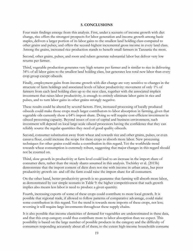
ANNEX A. PROCEDURE FOR DERIVATION OF LABOR FOR CROPS ON FIELDS WITH MULTIPLE CROPS
This procedure is needed because the Tanzania NPS gives labor only at the field level. The procedure first computes LQ ratios for all fields with one crop, then uses relative LQ ratios across crops from this calculation to take advantage of the data for total labor at the hh-field level, to allocate total L on the field to specific crops.
A.1. Summary for Coding in Stata
A.2. Derivations and Numerical Example (See Accompanying Excel File to Show That the Numerical Example Works out Properly)
1. Compute 𝐿𝐿𝑖𝑖 𝑄𝑄𝑖𝑖� for all cases with 1 crop per field
2. Note that 𝐿𝐿 = ∑ 𝐿𝐿𝑖𝑖𝑄𝑄𝑖𝑖𝑄𝑄𝑖𝑖𝑖𝑖 where L = total labor on the field (known), Qi = production of crop
i on field (known), and Li = labor on crop i on the field (unknown) 3. For fields with 2 crops: L = 𝐿𝐿1
𝑄𝑄1𝑄𝑄1 + 𝐿𝐿2
𝑄𝑄2𝑄𝑄2, where L, Q1 and Q2 are known and L1 and L2 are
unknown 4. For field with 3 crops: L = 𝐿𝐿1
𝑄𝑄1𝑄𝑄1 + 𝐿𝐿2
𝑄𝑄2𝑄𝑄2 + 𝐿𝐿3
𝑄𝑄3𝑄𝑄3 , where L, Q1, Q2, and Q3 are known and
L1, L2, and L3 are unknown 5. Note that relative LQ ratios can be computed from results in step #1. Let the relative LQ
ratio between crop 1 and crop 2 on a field �𝐿𝐿1𝑄𝑄1
𝐿𝐿2𝑄𝑄2
� � be denoted as LQ1,2 and so forth for
other LQ ratios 6. To build this around a numerical example, assume:
a. LQ1 = 0.9 b. LQ2 = 0.8 c. LQ3 = 0.7 d. Q1 = Q2 = Q3 = 1000 (set all equal for ease of exposition)
1. Case of two crops on a field, two steps:
i. From #8: 𝐿𝐿2 = 𝑄𝑄2𝐿𝐿�𝐿𝐿𝑄𝑄1,2𝑄𝑄1+ 𝑄𝑄2�
ii. L1 = L – L2 2. Case of three crops on a field, three steps:
i. From #10: 𝐿𝐿2 = 𝑄𝑄2𝐿𝐿
�𝐿𝐿𝑄𝑄1,2𝑄𝑄1+ 𝑄𝑄2+ 𝑄𝑄3𝐿𝐿𝑄𝑄2,3
�
ii. From #11: 𝐿𝐿1 = 𝐿𝐿𝑄𝑄1,2𝐿𝐿2𝑄𝑄2𝑄𝑄1
iii. L3 = L – L1 – L2

22
7. So:
a. LQ1,2 = 𝐿𝐿1𝑄𝑄1
𝐿𝐿2𝑄𝑄2
� = 0.9/0.8 = 1.125, meaning that 𝐿𝐿1𝑄𝑄1
= 1.125 𝐿𝐿2𝑄𝑄2
b. LQ2,3 = 𝐿𝐿2𝑄𝑄2
𝐿𝐿3𝑄𝑄3
� = 0.8/0.7 = 1.143, meaning that 𝐿𝐿3𝑄𝑄3
=𝐿𝐿2𝑄𝑄2
1.143�
8. From #3 (case of two crops), 𝐿𝐿 = 𝐿𝐿1𝑄𝑄1𝑄𝑄1 + 𝐿𝐿2
𝑄𝑄2𝑄𝑄2
= 1.125𝐿𝐿2𝑄𝑄2
𝑄𝑄1 + 𝐿𝐿2𝑄𝑄2
𝑄𝑄2
= 𝐿𝐿2𝑄𝑄2
(1.125𝑄𝑄1 + 𝑄𝑄2) ==> 𝐿𝐿2 = 𝑄𝑄2𝐿𝐿(1.125𝑄𝑄1+ 𝑄𝑄2) = 47.06
9. So L1 = L – L2 = 100 – 47.06 = 52.96. ** Note that the ratio of L1 to L2 is 52.96/47.06 = 1.125, which must be the case since Q1 = Q2.
10. From #4 (case of three crops), 𝐿𝐿 = 𝐿𝐿1𝑄𝑄1𝑄𝑄1 + 𝐿𝐿2
𝑄𝑄2𝑄𝑄2 + 𝐿𝐿3
𝑄𝑄3𝑄𝑄3
= 1.125𝐿𝐿2𝑄𝑄2
𝑄𝑄1 + 𝐿𝐿2𝑄𝑄2
𝑄𝑄2 + 𝐿𝐿2 𝑄𝑄2⁄1.143
= 𝐿𝐿2𝑄𝑄2�1.125𝑄𝑄1 + 𝑄𝑄2 + 𝑄𝑄3
1.143� ==> 𝐿𝐿2 = 𝑄𝑄2𝐿𝐿
�1.125𝑄𝑄1+ 𝑄𝑄2+ 𝑄𝑄31.143�
= 33.33
11. From 7a: 𝐿𝐿1𝑄𝑄1
= 1.125 𝐿𝐿2𝑄𝑄2
, 𝐿𝐿1 = 1.125 𝐿𝐿2𝑄𝑄2𝑄𝑄1 = 37.50
12. So L3 = L – L1 – L2 = 29.16 ** note that the ratio of L1 to L3 = 1.143, which must be the case since Q1 = Q2 = Q3
13. Computing the crop-specific Ls in this way, and knowing already the Qs, we take advantage of data on total L on field, and Q for each crop, to compute LQ ratios.
14. For coding in stata, we simply replace, in the key steps above, the numerical values we provided for LQ1,2 and LQ2,3 with these terms (which will be computed from actual data, just as the L and the crop-specific Qs will be):
a. Case of two crops on a field, two steps: i. From #8: 𝐿𝐿2 = 𝑄𝑄2𝐿𝐿
�𝐿𝐿𝑄𝑄1,2𝑄𝑄1+ 𝑄𝑄2�
ii. L1 = L – L2 b. Case of three crops on a field, three steps:
i. From #10: 𝐿𝐿2 = 𝑄𝑄2𝐿𝐿
�𝐿𝐿𝑄𝑄1,2𝑄𝑄1+ 𝑄𝑄2+ 𝑄𝑄3𝐿𝐿𝑄𝑄2,3
�
ii. From #11: 𝐿𝐿1 = 𝐿𝐿𝑄𝑄1,2𝐿𝐿2𝑄𝑄2𝑄𝑄1
iii. L3 = L – L1 – L2

23
ANNEX B. METHODS TO CONVERT CONSUMER FOOD EXPENDITURE FROM LSMS EXPENDITURE MODULES INTO LABOR AND VALUE OF PRODUCTION
ACROSS FARMING ACTIVITIES
Table B1. Parameters for Calculations of Farm Share of Consumer Expenditure
Item Factor Own production farm share 100% Unprocessed non-perishable farm share: 40% Unprocessed perishable farm share: 30% Low processed mfg share: 33% High processed mfg share: 50% Food away post-farm share 50%
Source: Authors.
Table B2. Resulting Factors by Source X Perishability X Processing Categories
Source x perishability x processing Category Farm share of
retail value Own production perishable 1.00 Own production non-perishable 1.00 Un-processed perishable 0.30 Un-processed non-perishable 0.40 Low processed perishable 0.20 Low processed non-perishable 0.27 High processed perishable 0.15 High processed non-perishable 0.20 Food away from home 0.15
Source: Authors.
24
Figure B1. View of Spreadsheet Deriving Farm Labor and Production from Consumer Expenditure (Part 1) Consumer demand
Commodity Groups (i)Own production
perishableOwn production non-perishable
Un-processed perishable
Un-processed non-perishable
Low processed perishable
Low processed non-perishable
High processed perishable
High processed non-perishable
Food away from home Total
Wheat and rice 6,300,000 231,600,000 - 69,000,000 - 1,920,000,000 529,000,000 40,800,000 533,000,000 3,329,700,000 All other cereals 90,300,000 1,184,000,000 48,900,000 264,000,000 - 1,640,000,000 1,055,083 300,000,000 1,190,000,000 4,718,255,083 Pulses 15,960,000 395,200,000 293,000,000 956,000,000 - - - - 354,000,000 2,014,160,000 Roots and tubers 345,000,000 - 563,000,000 - 163,000,000 - - - 277,000,000 1,348,000,000 Oilseeds 6,480,000 7,840,000 - - - - 25,600,000 1,020,000,000 164,000,000 1,223,920,000 Fruit 345,000,000 2,315,535 840,000,000 - - - 12,300,000 22,200,000 672,000,000 1,893,815,535 Vegetables 151,500,000 - 1,570,000,000 - - - 40,900,000 - 326,000,000 2,088,400,000 Poultry & eggs 257,400,000 - 92,200,000 - 324,000,000 - 79,000,000 38,700,000 189,000,000 980,300,000 Other meat 111,000,000 - - - 1,950,000,000 - - - 328,000,000 2,389,000,000 Dairy 183,300,000 - - - - - 533,000,000 - 141,000,000 857,300,000 Fish 30,600,000 - 820,000,000 - 1,442,249 - 442,000,000 - 244,000,000 1,538,042,249 Other food 1,134,812 37,160,000 - 51,300,000 - 1,240,000,000 104,000,000 558,000,000 2,180,000,000 4,171,594,812
All activities: 1,543,974,812 1,858,115,535 4,227,100,000 1,340,300,000 2,438,442,249 4,800,000,000 1,766,855,083 1,979,700,000 6,598,000,000 26,552,487,679
590
Cost build-up factors (Cf)
Own production perishable
Own production non-perishable
Un-processed perishable
Un-processed non-perishable
Low processed perishable
Low processed non-perishable
High processed perishable
High processed non-perishable
Food away from home
Farm share of retail value 1.00 1.00 0.30 0.40 0.20 0.27 0.15 0.20 0.15Import share 0.00 0.00 0.01 0.70 0.01 0.04 0.02 0.57 0.00
Consumer D at farm gate (Vif' and Vi')
Own production perishable
Own production non-perishable
Un-processed perishable
Un-processed non-perishable
Low processed perishable
Low processed non-perishable
High processed perishable
High processed non-perishable
Food away from home Total (Vi')
Wheat and rice 6,300,000 231,600,000 - 8,313,635 - 493,428,200 77,480,696 3,487,481 79,950,000 900,560,013 All other cereals 90,300,000 1,184,000,000 14,592,197 31,808,692 - 421,469,921 154,534 25,643,244 178,500,000 1,946,468,588 Pulses 15,960,000 395,200,000 87,433,819 115,186,020 - - - - 53,100,000 666,879,839 Roots and tubers 345,000,000 - 168,004,233 - 32,526,413 - - - 41,550,000 587,080,646 Oilseeds 6,480,000 7,840,000 - - - - 3,749,538 87,187,031 24,600,000 129,856,570 Fruit 345,000,000 2,315,535 250,663,509 - - - 1,801,536 1,897,600 100,800,000 702,478,180 Vegetables 151,500,000 - 468,502,035 - - - 5,990,473 - 48,900,000 674,892,509 Poultry & eggs 257,400,000 - 27,513,304 - 64,653,730 - 11,570,841 3,307,979 28,350,000 392,795,853 Other meat 111,000,000 - - - 389,119,668 - - - 49,200,000 549,319,668 Dairy 183,300,000 - - - - - 78,066,562 - 21,150,000 282,516,562 Fish 30,600,000 - 244,695,330 - 287,799 - 64,738,124 - 36,600,000 376,921,254 Other food 1,134,812 37,160,000 - 6,181,007 - 318,672,379 15,232,500 47,696,435 327,000,000 753,077,133
All activities 1,543,974,812 1,858,115,535 1,261,404,429 161,489,354 486,587,610 1,233,570,501 258,784,806 169,219,770 989,700,000 7,962,846,816
------------------ Cost build-up factors (Cf) ------------------
-------------------- Farm gate value of consumer expenditure (V'if = Vif * Cf) ------------------
-------------------- Value of consumer expenditure (Vif) ------------------
2010Food expenditure categories (f)
V'if = Vif * Cf * (1-If)
25
Figure B1. View Of Spreadsheet Deriving Farm Labor And Production From Consumer Expenditure (Part 2) Consumer D at farm gate (Vif' and Vi')
Own production perishable
Own production non-perishable
Un-processed perishable
Un-processed non-perishable
Low processed perishable
Low processed non-perishable
High processed perishable
High processed non-perishable
Food away from home Total (Vi')
Wheat and rice 6,300,000 231,600,000 - 8,313,635 - 493,428,200 77,480,696 3,487,481 79,950,000 900,560,013 All other cereals 90,300,000 1,184,000,000 14,592,197 31,808,692 - 421,469,921 154,534 25,643,244 178,500,000 1,946,468,588 Pulses 15,960,000 395,200,000 87,433,819 115,186,020 - - - - 53,100,000 666,879,839 Roots and tubers 345,000,000 - 168,004,233 - 32,526,413 - - - 41,550,000 587,080,646 Oilseeds 6,480,000 7,840,000 - - - - 3,749,538 87,187,031 24,600,000 129,856,570 Fruit 345,000,000 2,315,535 250,663,509 - - - 1,801,536 1,897,600 100,800,000 702,478,180 Vegetables 151,500,000 - 468,502,035 - - - 5,990,473 - 48,900,000 674,892,509 Poultry & eggs 257,400,000 - 27,513,304 - 64,653,730 - 11,570,841 3,307,979 28,350,000 392,795,853 Other meat 111,000,000 - - - 389,119,668 - - - 49,200,000 549,319,668 Dairy 183,300,000 - - - - - 78,066,562 - 21,150,000 282,516,562 Fish 30,600,000 - 244,695,330 - 287,799 - 64,738,124 - 36,600,000 376,921,254 Other food 1,134,812 37,160,000 - 6,181,007 - 318,672,379 15,232,500 47,696,435 327,000,000 753,077,133
All activities 1,543,974,812 1,858,115,535 1,261,404,429 161,489,354 486,587,610 1,233,570,501 258,784,806 169,219,770 989,700,000 7,962,846,816
Labor:output ratios (LQi) LQi Total (Vi')Wheat and rice 0.152 900,560,013 labor days Value of prodnAll other cereals 0.274 1,946,468,588 137,139,581 900,272,534 Pulses 0.311 666,879,839 526,132,136 1,923,428,030 Roots and tubers 0.282 0.564 587,080,646 195,108,687 627,244,617 Oilseeds 0.151 129,856,570 82,097,968 164,166,476 Fruit 19,123,745 126,992,211 Vegetables 0.078 674,892,509 Poultry & eggs 12,483,007 160,169,076 Other meat 972,085,124 3,902,272,944 DairyFishOther food
4,905,738,165
Computed labor on farm (L'i = Vi' * LQi)
Commodity Groups (i)
L'i (total person days
of labor; '000) Scaled L'i
Wheat and rice 137,183 119,627,365 All other cereals 532,435 464,296,432 Pulses 207,437 180,890,729 Roots and tubers 165,535 144,350,658 Oilseeds 19,555 17,052,531 Fruit - - Vegetables 52,599 972,085,124 45,867,409 Poultry & eggs - - Other meat - - Dairy - - Fish - - Other food - -
All activities 1,114,744 972,085,124
Days from LSMS farm labor modules
-------------------- Farm gate value of consumer expenditure (V'if = Vif * Cf) ------------------
From NPS farm module
Li' = Vi' * LQi
Scaling
26
REFERENCES
Arthi, V., K. Beegle, J. De Weerdt, and A. Palacios-Lopez. 2013. Not Your Average Job: Irregular Schedules, Recall Bias, and Farm Labor Measurement in Tanzania. Washington, DC: World Bank.
Dolislager, M. Forthcoming. Food Consumption Patterns in Light of Rising Incomes, Urbanization, and Food Retail Modernization: Evidence from East and Southern Africa. Ph.D. dissertation. Michigan State University.
Gibson, J., K. Beegle, J. De Weerdt, and J. Friedman. 2015. What Does Variation on Household Survey Methods Reveal about the Nature of Measurement Errors in Consumption Estimates? Oxford Bulletin of Economics and Statistics 77.3: 319-474.
McCullough, Ellen B. 2015. Understanding Agricultural Labor Exits in Tanzania. Selected paper prepared for presentation at the 2015 Agricultural and Applied Economics Association and Western Agricultural Economics Association Annual Meeting, 26-28 July. San
Francisco, CA.
Radelet, S. 2010. Emerging Africa: How 17 Countries Are Leading the Way. Washington, DC: Center for Global Development.
Seto, K. and N. Ramankutty. 2016. Hidden Linkages between Urbanization and Food Systems. Science 352.6288: 943-945.
Tanzania. 2010/11. N ational Park Survey data. http://www.nbs.go.tz/tnada/index.php/catalog/15/overview.
Tschirley, D., J. Snyder, J. Goeb, M. Dolislager, T. Reardon, S. Haggblade, L. Traub, F. Ejobi, and F. Meyer. 2015a. Africa’s Unfolding Diet Transformation: Implications for Agrifood System Employment. Journal of Agribusiness in Developing and Emerging Economies 5.2: 102-136.
Tschirley, David, Michael Dolislager, Thomas Reardon, and Jason Snyder. 2015b. The Rise of the African Middle Class: Projections and Implications in East and Southern Africa to 2040. Journal of International Development 27.5. 628–646.
World Bank. 2014. Sustaining Economic Growth in Africa: State of the Africa Region. World Bank-IMF Spring Meetings April 2014. http://live.worldbank.org/state-of-the-africa-region
Young, Alwyn. 2012. The African Growth Miracle. Journal of Political Economy. 120.4: 696-739.

www.feedthefuture.gov


