
FDD Evaluator 0.1 Draft Software documentation and technical background
January 11, 2013
Developed at Ray W. Herrick Laboratories
Purdue University
Jim Braun - [email protected]
David Yuill - [email protected]
Research and Results Supported by:

Documentation for FDD Evaluator 0.1 January 11, 2013 Page ii
Contents
Using FDD Evaluator 0.1 ............................................................................................................................. 1
Acknowledgements ............................................................................................................................... 1
About FDD Evaluator 0.1 ......................................................................................................................... 1
Disclaimer ............................................................................................................................................. 1
Use ........................................................................................................................................................ 1
Installing FDD Evaluator .......................................................................................................................... 2
Using FDD Evaluator ............................................................................................................................... 2
Select Input Details ................................................................................................................................... 3
Select the units to be used in the evaluation ......................................................................................... 3
Select the fault conditions ..................................................................................................................... 3
Enter limits for operating conditions .................................................................................................... 4
Select protocol to evaluate .................................................................................................................... 4
Control buttons.......................................................................................................................................... 4
Evaluate................................................................................................................................................. 4
Exit ........................................................................................................................................................ 5
Software Outputs ...................................................................................................................................... 5
Detailed description of evaluation process ............................................................................................... 6
Input Data Library ......................................................................................................................................... 7
Faults ......................................................................................................................................................... 7
Faults considered in this project ............................................................................................................ 7
Imposing faults in laboratory experiments ............................................................................................ 8
Summary of data library ..................................................................................................................... 10
Charge effect on COP and capacity .................................................................................................... 14
Normal model & FIR .......................................................................................................................... 16
Evaluation Method ...................................................................................................................................... 20
Approach summary ............................................................................................................................. 20
Faulted and unfaulted operation .......................................................................................................... 21
Test case outcomes ............................................................................................................................. 21
Test case outcome rate calculations .................................................................................................... 23
Case Study .................................................................................................................................................. 25

Documentation for FDD Evaluator 0.1 January 11, 2013 Page iii
RCA background .................................................................................................................................... 25
RCA versions: 2008, 2013, Installer & HERS ................................................................................... 26
Test results .............................................................................................................................................. 27
No Response ....................................................................................................................................... 27
False Alarm ......................................................................................................................................... 28
Misdiagnosis ....................................................................................................................................... 32
Missed Detections ............................................................................................................................... 38
Conclusions of case study ................................................................................................................... 43
Nomenclature and references ...................................................................................................................... 45
Definitions............................................................................................................................................... 45
Terminology ............................................................................................................................................ 45
References ............................................................................................................................................... 47
Appendix A – Capacity and COP vs. charge plots ..................................................................................... 48
Capacity vs. charge plots ........................................................................................................................ 52

Documentation for FDD Evaluator 0.1 January 11, 2013 Page 1
Using FDD Evaluator 0.1
FDD Evaluator 0.1 is a standalone self-extracting software application designed for computers equipped
with the Windows operating system. The purpose of this software is to evaluate the performance of
fault detection and diagnostics (FDD) protocols that are intended to be deployed on air-cooled unitary
air-conditioning equipment.
Acknowledgements
We are grateful to Mark Cherniack of New Buildings Institute (NBI) and Drs. Vance Payne and Piotr
Domanski of the US National Institute of Standards and Technology (NIST) for overseeing this project,
and to the California Energy Commission (CEC) and NIST for funding that supported the work and the
development of this software.
About FDD Evaluator 0.1
FDD Evaluator 0.1 was written by David Yuill under the supervision of Jim Braun of Purdue University. It
was completed in January 2013 as part of two projects focused on development of FDD evaluation
methods. These projects were funded by CEC, through NBI, and by NIST.
The distribution rights of this software are held jointly by CEC and NIST. Any requests to distribute this
software should be made to both agencies. All other requests regarding this software should be made to
either CEC or NIST. Purdue University is not responsible for upkeep or repair of this software.
Disclaimer
THE SOFTWARE IS PROVIDED "AS IS", WITHOUT WARRANTY OF ANY KIND, EXPRESS OR IMPLIED,
INCLUDING BUT NOT LIMITED TO THE WARRANTIES OF MERCHANTABILITY, FITNESS FOR A PARTICULAR
PURPOSE AND NONINFRINGEMENT. IN NO EVENT SHALL THE AUTHORS OR PURDUE UNIVERSITY BE
LIABLE FOR ANY CLAIM, DAMAGES OR OTHER LIABILITY, WHETHER IN AN ACTION OF CONTRACT, TORT
OR OTHERWISE, ARISING FROM, OUT OF OR IN CONNECTION WITH THE SOFTWARE OR THE USE OR
OTHER DEALINGS IN THE SOFTWARE. WE MAKE NO CLAIM OF THE ABILITY OF THE SOFTWARE TO
FOLLOW THE EVALUATION PROCEDURE, NOR TO THE EFFECTIVENESS OF THE EVALUATION METHODS.
Use
By installing this software you are agreeing to the following terms and conditions. You may not use this
software for a paid service, nor incorporate the documentation, software, or any portions of the
documentation or software into any commercial products. This software may be used to aid in
development of commercial products.
FDD Evaluator 0.1 may be referenced as follows:

Documentation for FDD Evaluator 0.1 January 11, 2013 Page 2
Yuill, D. P and J.E. Braun (2013). FDD Evaluator (Version 0.1) [Software]. West Lafayette, IN: Purdue
University.
Installing FDD Evaluator
The file FDD_Evaluator_01_pkg.exe is a self-extracting package for Windows operating systems. This
package includes all of the files required to run the software, and includes a C compiler developed by
Matlab, called MCR. You will be prompted to install this on your machine. After the installer has
completed the installation, launch the software from the executable file FDD_Evaluator.exe.
Using FDD Evaluator
When the executable file is launched, a user interface screen, shown in Figure 1, opens. The user
interface allows the user to select details about the inputs used in the evaluation, and to select the
protocol to be evaluated. In version 0.1 there are four built-in protocols that are included with the
software, described below. Once the inputs and candidate protocol are selected, clicking the “Evaluate”
button will run the evaluation process and launch figures and tables showing the outcomes of the
evaluation.
Figure 1: FDD Evaluator 0.1 user interface

Documentation for FDD Evaluator 0.1 January 11, 2013 Page 3
Select Input Details
The user can limit the input data by selecting only certain air-conditioning systems from the database, or
certain fault types, or certain driving conditions.
Select the units to be used in the evaluation
The nine test units can be selected by clicking the radio buttons. If the top button, “ALL”, is selected,
then all units will be used. Some details about the units are shown in a table below the radio buttons.
Table 1: Description of labels in unit selection table on the FDD Evaluator interface
Label Description
Unit ID Unique identifier for the unit
Config. Rooftop unit or split system
Size (tons) Nominal system capacity in tons
Refrig. Working fluid (refrigerant) type
Expansion Metering device type; either fixed orifice (FXO) thermostatic expansion valve (TXV)
Compressor Compressor type; either scroll or reciprocating (Recip.)
Further detail about the units is provided below in the detailed description of the evaluation process.
Select the fault conditions
These buttons allow input data to be filtered according to the fault imposed by the experimenter. For
example, the user may select only tests with undercharge faults (UC). The user may also select only
those tests for which no fault was imposed (Unfaulted). If the “ALL” button is selected, then all fault
types will be included.
The following table lists brief descriptions for the fault type abbreviations. Further detail describing
these faults can be found in the detailed description of the evaluation process.
Table 2: Brief description of fault types
Button Description
ALL All fault types will be included
Unfaulted Tests with no fault imposed
EA Evaporator (indoor coil) airflow fault
CA Condenser (outdoor coil) airflow fault
UC Undercharge of refrigerant
OC Overcharge of refrigerant
LL Liquid line restriction
NC Non-condensables in the refrigerant
VL Compressor valve leakage

Documentation for FDD Evaluator 0.1 January 11, 2013 Page 4
Enter limits for operating conditions
The input data come from experiments conducted across a range of operating conditions (ambient dry-
bulb temperature, indoor dry-bulb temperature, and indoor humidity). The input tests can be limited to
only include those tests done within a narrower range. This is done by entering temperatures, in °F, into
the cells. The default values that appear in the text boxes will span the entire data set, so entering a
lower minimum or higher maximum than the default value will have no effect.
Table 3: Description of user-entered operating conditions
Text box Description Default
Min. ambient Minimum ambient (outdoor) air dry bulb temperature [°F] 59
Max. ambient Maximum ambient (outdoor) air dry bulb temperature [°F] 128
Min. IA dry bulb Minimum indoor air dry bulb temperature [°F] 67
Max. IA dry bulb Maximum indoor air dry bulb temperature [°F] 84
Min. IA wet bulb Minimum indoor air wet bulb temperature [°F] 51
Max. IA wet bulb Maximum indoor air wet bulb temperature [°F] 74
Note 1: The following actions will result in an error:
Entering a minimum value higher than or equal to the maximum value
Leaving a text box blank
Entering a non-numeric value in a text box
Note 2: Numbers with up to 16 digits may be entered (e.g. 95.000000000001 is a legal entry).
Select protocol to evaluate
This dropdown menu allows selection of a protocol that can be evaluated. Built-in protocols are
programmed into the following files:
RCA_2008
RCA_2008_HERS
RCA_2013
RCA_2013_HERS
These FDD protocols are described in the detailed description that follows.
Control buttons
Two additional buttons control the evaluator, and are described below.
Evaluate
Clicking this button runs the evaluation. Once the evaluation is complete, the outputs (described below)
will pop up.

Documentation for FDD Evaluator 0.1 January 11, 2013 Page 5
Exit
The “Exit” button closes the software. Inputs are not saved.
Software Outputs
When an evaluation is conducted, the results are provided in two forms:
1) A series of plots showing the False Alarm, Misdiagnosis and Missed Detection rates as a function
of the fault impact
2) A series of tables showing the numerical data that form the basis of the plots. The numerical
results also contain the sample sizes and No Response rate. These tables are formatted to allow
the values to be easily copied and pasted, so that users may conduct meta-analyses in software
platforms of their choice.
An example output, showing the results of an evaluation of the 2008 RCA protocol using the full data set
of 607 tests, is shown below.

Documentation for FDD Evaluator 0.1 January 11, 2013 Page 6
Figure 2: FDD Evaluator 0.1 outputs
Detailed description of evaluation process
The remainder of this documentation package contains excerpts from final reports on the FDD
evaluation projects, which were submitted to NBI and NIST.

Detailed description of evaluation process – excerpted from final reports
Documentation for FDD Evaluator 0.1 January 11, 2013 Page 7
Input Data Library
A library of Fault/No Fault data has been compiled. These data represent unitary systems operating with
and without faults over a range of conditions, and they constitute the inputs that are fed to the candidate
FDD protocols when evaluating their performance. This section describes the faults that are represented
in the library, a description of the attributes of the data, and a description of the vetting and augmentation
of the data library to meet the needs of this project.
Faults
Faults considered in this project
There are six degradation faults that are included in the evaluation. These six faults are listed in Table 4,
along with a description of each fault. A diagram showing the components of an air-conditioning system
is shown in Figure 3, and referred to in the descriptions of faults and how to impose faults in
experiments.
Table 4: Faults included in evaluation of FDD protocols
Fault Abbr. Description
Under- or overcharge UC, OC A mass of refrigerant that is less or more than the manufacturer specification
Low-side heat transfer EA Faults in the evaporator coil such as coil fouling or insufficient airflow
High-side heat transfer CA Faults in the condenser coil such as coil fouling or insufficient airflow
Liquid line restriction LL Flow restrictions such as crimps or fouled filter/drier in the liquid line (Figure 3)
Non-condensables NC The presence of gases that do not condense (e.g. air or nitrogen) in the refrigerant
Compressor valve leakage VL Leaks in the compressor from high to low pressure regions, reducing mass flow

Detailed description of evaluation process – excerpted from final reports
Documentation for FDD Evaluator 0.1 January 11, 2013 Page 8
Figure 3: Components of a typical vapor-compression air-conditioner
Imposing faults in laboratory experiments
To provide measurement data as an evaluator input, faults were simulated in a laboratory. We have
selected a term to quantify the severity of the fault – Fault Intensity (FI) – and defined FI for each type of
fault. A description of how faults were imposed in the laboratory, and the definition of FI for each fault
type is provided below.
1. Charge: To impose an under- or overcharge fault, charge is simply removed from or
added to the system. The fault intensity is:
(1)
where mactual is the measured mass of refrigerant in the system
mnominal is the nominally correct mass of refrigerant (see discussion on charge
effect on COP and capacity on page 14)
Thus a system designed for 5 lb of charge that had 4.5 lb would be referred to as 10%
undercharged or having FIcharge = -10%. If manufacturer specifications are not available, an
alternate definition for nominal mass can be based on the refrigerant mass that provides the
maximum capacity or efficiency.
2. Low-side heat transfer faults: In a typical laboratory setup the airflow across the
evaporator coil can be modulated using a variable speed booster fan or dampers. Reducing
the airflow accurately duplicates the effect of most faults in this category: airflow reduction
from fan or distribution system design problems, obstructions or filter fouling. The effect of
evaporator coil air-side fouling is also assumed to be well represented by reducing airflow,

Detailed description of evaluation process – excerpted from final reports
Documentation for FDD Evaluator 0.1 January 11, 2013 Page 9
particularly if the fouling is assumed to be evenly distributed across the face of the heat
exchanger. The fault intensity is defined analogously to FIcharge using either mass flow rate or
volumetric airflow rate.
(2)
3. High-side heat transfer faults: Similar to low-side faults, a reduction in airflow is used to
implement high-side heat transfer faults. Some experimenters have simulated blockage by
large-scale debris, such as leaves, by covering the face of the condenser coil with paper or
mesh. Although this may, in some cases, more realistically represent the fault physically, it
is not repeatable nor easily quantified as a fault intensity. Furthermore, the general effect –
to increase the refrigerant’s high-side pressure – is the same as with reduced airflow.
Therefore, reduced airflow is proposed as the standard means of imposing this fault in the
laboratory. Accordingly, the fault intensity is defined with airflow rates in the same manner
as with low-side heat transfer faults.
(3)
4. Liquid line restriction: A liquid line restriction is implemented by using one or more
valves to impose the desired pressure loss. The fault intensity is defined using the ratio of
the increase in pressure drop through the liquid line caused by the faulted condition to the
liquid line pressure drop under non-faulted operation and at the same operating condition.
(4)
5. Non-condensables in the refrigerant: A non-condensables fault is imposed by
introducing nitrogen into the refrigerant line. The maximum amount of non-condensables
to be expected is in the case where a system has been open to the atmosphere and not
evacuated prior to charging. Therefore, the fault is defined with a mass of nitrogen
compared to the mass of nitrogen that would fill the system at atmospheric pressure.
(5)
6. Compressor valve leakage: Compressor valve leakage is simulated with the use of a hot
gas bypass – a pipe carrying refrigerant from the discharge to the inlet of the compressor
(from point 1 to point 5 in Figure 3). The fault intensity for this fault is defined as the change
in mass flow rate (at a given operating condition) to the original mass flow rate.

Detailed description of evaluation process – excerpted from final reports
Documentation for FDD Evaluator 0.1 January 11, 2013 Page 10
(6)
Summary of data library
Table 5 shows a summary of the units and numbers of test cases contained in the experimental data
library. The number of tests is separated to show the number for each fault type for each system, using
the fault type abbreviations given in Table 4. There are a total of 607 test cases, gathered from
experiments on nine unitary systems. Three of the systems are rooftop units (RTU), but the tests on
these three make up 60% of the total test cases.
Table 5: Summary of test cases in experimental data library
Note 1: RTU 2 is a split system, but was named using a previous naming convention.
The rightmost columns show the limits of the range of ambient temperature during testing for each of
the test units in the library. The distribution of tests by return air wet-bulb temperature and by ambient
temperature (among the entire set of 607) is shown in Table 6.
Number of tests
# ID Type
Capacity
[tons] Refrig.
Exp.
Device
Comp.
Type
No
Fault UC OC EA CA LL NC VL
1 RTU 3 RTU 3 R410a FXO Scroll 24 25 12 21 6 0 0 067 125
2 RTU 7 RTU 3 R22 FXO Recip. 39 34 0 26 36 34 0 33 60 100
3 RTU 4 RTU 5 R407c FXO Scroll 17 15 12 19 8 0 0 067 116
4 Split 1 Split 3 R410a FXO Recip. 1 29 1 0 0 0 0 082 127
5 RTU 21 Split 2.5 R410a TXV Scroll 16 12 12 21 15 16 15 1670 100
6 Split 2 Split 3 R410a TXV Recip. 2 30 7 0 0 0 0 083 127
7 Split 3 Split 3 R410a TXV Scroll 4 4 7 0 0 0 0 082 125
8 Split 4 Split 3 R22 TXV Scroll 4 8 0 8 0 0 0 0 82 125
9 Split 5 Split 3 R22 TXV Scroll 4 4 4 6 0 0 0 0 82 125
Total: 111 161 55 101 65 50 15 49
Ambient
Temp.
Min. Max.
[°F] [°F]

Detailed description of evaluation process – excerpted from final reports
Documentation for FDD Evaluator 0.1 January 11, 2013 Page 11
Table 6: Distribution of tests by return air wet-bulb temperature (left) and ambient temperature (right)
Description of data
The data in the library represent steady-state cooling operation. Each datum is an average of multiple
measurements – from 8 to several hundred – taken while the equipment was operating steadily. The
experimenters followed the same standards that equipment performance rating experiments follow,
such as AHRI Standard 210/240 (AHRI 2008) and ASHRAE Standard 37 (ASHRAE 2009). More details on
the experimental approaches of the data included in the data library can be found in the following
references: Breuker (1997), Kim et al. (2006), Shen et al. (2006), Palmiter et al. (2011).
The data library contains measurement data and system information. The types of measurement (and
calculated) data are listed in Table 7 in IP units. The entire data library also has an SI-unit version so that
inputs are readily available for protocols that use these units, such as European protocols.
Table 7: Data library measurement data types
Variable ID IP Units Description
T_RA [°F] Return Air dry bulb temperature (evaporator inlet)
DP_RA [°F] Return Air dewpoint temperature (evaporator inlet)
WB_RA [°F] Return Air wet bulb temperature (evaporator inlet)
RH_RA [%] Return Air relative humidity (evaporator inlet)
T_SA [°F] Supply Air dry bulb temperature (evaporator outlet)
DP_SA [°F] Supply Air dewpoint temperature (evaporator outlet)
WB_SA [°F] Supply Air wet bulb temperature (evaporator outlet)
RH_SA [%] Supply Air relative humidity (evaporator outlet)
T_amb [°F] Ambient air dry bulb temperature
P_LL [psia] Liquid line pressure
T_LL [°F] Liquid line temperature
P_suc [psia] Suction pressure
T_suc [°F] Suction temperature
P_dischg [psia] Compressor discharge pressure
T_dischg [°F] Compressor discharge temperature
Return air wet-bulb Ambient Temperature
Range Number of Range Number of
[°F] occurrences [°F] occurrences
50-55 16 60-70 53
55-60 260 70-80 58
60-65 85 80-90 223
65-70 240 90-100 186
70-75 6 100-110 26
607 110-120 39
>120 22
607

Detailed description of evaluation process – excerpted from final reports
Documentation for FDD Evaluator 0.1 January 11, 2013 Page 12
Power [W] Total electrical power of system
T_air_ce [°F] Condenser exiting air temperature
T_sat_e [°F] Refrigerant saturation temperature in the evaporator
T_sat_c [°F] Refrigerant saturation temperature in the condenser
Power_comp [W] Compressor power
Fault [ - ] Experimenter’s identified fault type (or unfaulted)
Q_ref [Btu/hr] Refrigerant side capacity
Q_air [Btu/hr] Air-side capacity
SHR [-] Sensible Heat Ratio
COP [-] Coefficient of performance
SH [°F] Suction Superheat
SC [°F] Subcooling
m_ref [lbm/min] Refrigerant mass flow rate
Chrg [lbm] Mass of refrigerant charge
Chrg% [%] Charge as a percentage of nominally correct charge
V_i [CFM] Indoor coil volumetric airflow rate
V_i_nom [CFM] Nominal indoor coil volumetric airflow rate
V_i_% [%] Indoor coil volumetric airflow rate as percentage of nominal
V_o [CFM] Outdoor coil volumetric airflow rate
V_o_nom [CFM] Nominal outdoor coil volumetric airflow rate
V_o_% [%] Outdoor coil volumetric airflow rate as a percentage of nominal
Blk% [%] Portion of outdoor coil blocked
LL restr. [psia] Pressure loss through liquid line restriction
NonCond [lbm/lbm] Mass fraction of non-condensables in the refrigerant
NonCond% [%] Mass of non-condensables as a percentage of reference mass
VlvLeak [lbm/min] Compressor hot-gas bypass mass flow rate
VlvLeak [%] Compressor hot-gas bypass mass flow rate as % of total mass flow
FIRcapacity [%] Fault Impact Ratio for capacity
FIRCOP [%] Fault Impact Ratio for COP
For each test case there are also pieces of system information about the test unit. The types of system
information are described in Table 8.
Table 8: Data library system information
Variable ID Description
Expansion Type Expansion valve type (TXV, FXO or EEV)
Manufacturer Manufacturer
Model (indoor) Model of indoor unit (for split systems)
Model (outdoor) Split system outdoor unit model or RTU model
Nominal Capacity Nominal Capacity (tons)

Detailed description of evaluation process – excerpted from final reports
Documentation for FDD Evaluator 0.1 January 11, 2013 Page 13
Refrigerant Refrigerant
Operating Mode Cooling or heating
Compressor Type Reciprocating, scroll, etc.
Compressor Model Compressor Model
Target SC Target subcooling rate (for TXV systems)
EER Energy efficiency ratio
SEER Seasonal energy efficiency ratio
C1 to C10 Compressor map coefficients
Some of the test units in the data library do not have all of the types of data listed in these tables.
Data vetting, uncertainty and removal of questionable data
FDD protocols use different inputs to detect and diagnose faults. To ensure that the evaluations are
meaningful they must be fair, which requires consistent data. A great deal of effort has gone into
studying the data to look for inconsistencies because of the importance of using reliable input data. This
was done manually.
In conducting and reporting on experiments, results can’t be removed from the dataset without
justification because this could skew the overall results or conclusions of the experiment. However, in
vetting the data for the evaluator, removal of a test case doesn’t necessarily skew results because it is
removed for all protocols that will be evaluated.
Of more than 1000 test cases that were collected for 14 units, about 40% were removed. Some of the
reasons for removal:
Data that don’t follow physical laws – for example if significant refrigerant pressure increases
occur in locations other than the compressor, if energy is not conserved, humidity is generated
across the evaporator, etc.
Data that show too much scatter, or are obvious outliers when compared to other data within
the set. For unfaulted tests, a normal model (described below) was an effective tool for
assessing outliers. One of the test units was rejected completely because of questionable data.
Data that are not self-consistent – as with fault detection, redundancy in data can be used to
detect problems. For example, in cases where an experimenter provided two forms of humidity,
such as wet-bulb and relative humidity, each was checked using psychrometric relationships and
the associated pressure and dry-bulb temperature. If they didn’t agree, the test was further
investigated by comparing to air-side capacity or sensible heat ratio if sufficient data were
available. If it was unclear which variable was flawed, the test case was removed. Similar
approaches were used to check other calculated data, such as capacity and COP.

Detailed description of evaluation process – excerpted from final reports
Documentation for FDD Evaluator 0.1 January 11, 2013 Page 14
Insufficient data – some data sets did not contain enough data to determine the impact of a
fault. Four of the 14 test units were removed for this reason.
Charge effect on COP and capacity
For faults such as the presence of non-condensable gas in the refrigerant, compressor valve leakage, or
reduced airflow across the outdoor coil, the unfaulted condition is clear. However, the unfaulted or
“correct” mass of refrigerant charge in a system is less clear. The experimenters have charged their
experimental units by methods that they may not have detailed within their description of the
experiments. Their data sets usually identify which tests they consider to be conducted with correct
charge. However, when evaluating FDD protocols that are attempting to diagnose charge faults, it’s
imperative that the experiments with nominally correct charge truly have correct charge.
An earlier approach to defining the correct charge was to use the experimenters’ nominally correct
values. However, this was criticized because we can’t be certain that the experimenters’ values were
correct. To provide a consistent approach, we currently define the correct charge as being the mass of
charge that gives the maximum COP at the standard rating condition (95/80/67). In most cases this
approach agrees with the experimenter value. For example, consider Figure 4. Although the COP
flattens out around 100% of nominal charge for the rating condition (purple line), there is a point at
100% that gives the highest COP (2.5). However, there are four units in the data library for which the
experimenter’s nominally correct value gave the maximal capacity, but not the maximal COP.

Detailed description of evaluation process – excerpted from final reports
Documentation for FDD Evaluator 0.1 January 11, 2013 Page 15
Figure 41: Relative COP as a function of charge at three conditions for a FXO RTU
In the four test units for which the maximal COP at the rating condition was not reached at the
experimenter’s nominal charge, the nominal charge was updated to match the charge for which the
maximum COP was achieved. In this report “nominal charge” refers to the maximal-COP charge.
The updated nominal charge for the four units changes the fault category for many of the tests in the
affected dataset. One complication of this update is that the other fault test cases became multiple
fault cases. For example, cases with evaporator airflow faults imposed became evaporator airflow and
over-charge or under-charge fault cases. These tests were removed from the evaluation inputs.
1 Plots similar to Figure 4 showing the capacity and COP as a function of relative charge at the standard condition
and all other conditions for which there are sufficient data, have been generated for each applicable unit. These
are provided in Appendix A.
0
0.5
1
1.5
2
2.5
3
3.5
0.4 0.6 0.8 1 1.2 1.4
CO
P
Relative Charge
COP for RTU 4
82/80/60
82/80/67
95/80/67

Detailed description of evaluation process – excerpted from final reports
Documentation for FDD Evaluator 0.1 January 11, 2013 Page 16
Normal model & FIR
In six of the nine systems in the data library there was a sufficient set of no-fault tests to enable
development of a normal model2. The six modeled systems are numbered 1 to 6 in Table 5. A normal
model is a multiple linear regression of the driving conditions that predicts capacity or COP, as shown in
Eqs. 7 and 8, where the coefficients i and i are found using a least squares approach. The normal
model is developed using unfaulted tests (those with no faults imposed, and with maximal-COP charge),
so that it can be used to assess what the capacity or COP degradation is for faulted tests at any given
condition. The normal model approach for determining degradation is preferable to a measurement-
based approach for two reasons. The first is that it significantly reduces bias error, because it obviates
the problem of trying to exactly match the test conditions for a faulted and an unfaulted test. The
second is that it reduces or eliminates one half of the random error associated with a comparison of two
test results (faulted and unfaulted tests at the same conditions).
(7)
(8)
For wet-coil cases, the two external driving conditions are ambient air dry bulb and return air wet bulb
temperature. For dry-coil cases, the two driving conditions are ambient dry bulb and return air dry bulb.
To use a single two-input model (as shown in Eqs. 7 and 8) to represent both dry- and wet-coil cases, an
approach has been followed in which a fictitious return air wet bulb temperature, wbra,f , is used in place
of the actual return air wet bulb temperature, wbra for all dry-coil cases (see Brandemuehl (1993) for
details). This wbra,f is calculated using an iterative approach that involves a bypass factor (BF). BF
indicates the fraction of air that would need to bypass an ideal coil, , to give equivalent
performance to the real coil. Using energy and mass balances and psychrometric relationships, BF can
also be expressed in terms of specific enthalpies, h, or humidity ratios, , as shown in Eq. 9.
(9)
2 Systems 4 and 6 from Table 5 are among the four that had their nominal charge adjusted to give maximal COP at
the rating condition. These systems had a large number of tests conducted with the experimenter’s original
nominal charge, but only one or two tests with the maximal-COP charge. For these two cases the normal model
was developed using the original nominal charge. To adjust the FIR values for the updated nominal charge level,
each FIR value was divided by the FIR at the maximal-COP charge. For example, in system #4, the maximal-COP
charge gave a FIRCOP of 104%. Therefore, all FIRCOP values were divided by 104% when the nominally correct charge
level was adjusted. Although the resulting FIR values are not exact, this method correctly represents the trends
caused by adjusting charge, and the magnitude of the inaccuracies introduced by this method is small. The effect
of the inaccuracies on an FDD evaluation is insignificant.

Detailed description of evaluation process – excerpted from final reports
Documentation for FDD Evaluator 0.1 January 11, 2013 Page 17
For a wet coil condition, the air leaving an ideal coil will have a dewpoint temperature equal to the
surface temperature of the coil – the apparatus dewpoint (adp). In the fictitious wet bulb approach, BF
is iteratively varied until the enthalpy calculations of Eq. 9 give the same result as the humidity ratio
calculations with an assumption of 100% relative humidity for the air at the apparatus dewpoint.
The BF values calculated for the wet coil cases are averaged, and this average is then used to calculate
sensible heat ratios for each dry coil test using Eq. 10. In Eq. 10, adp is calculated using Eq. 9, and the
fictitious return air enthalpy, hra,f, is varied until SHR converges to 1.0. Finally, the fictitious wet bulb,
wbra,f , is calculated from hra,f and Tra and is used in Eqs. 7 and 8 for any dry coil cases in the data set.
(10)
This approach is described in more detail by Brandemuehl (1993).
During model validation, the measured unfaulted cases (the basis for the model) are compared with
model outputs for the same set of conditions. The capacity and COP are compared, and residuals
calculated. For example, Eq. 11 shows the calculation for capacity.
(11)
An example plot, showing the residuals for the normal model of capacity for RTU 3, is shown in Figure 5.
This plot indicates the level of scatter for this unit, which is typical for a laboratory-tested unit. The dry
coil and wet coil data are shown separately to illuminate any difference that could be caused by
problems associated with the fictitious wet-bulb approach to model generation. The wet and dry coil
cases are very similarly distributed, indicating that this modeling approach hasn’t introduced any
obvious bias or scatter error. The dry coil cases are associated with lower-capacity cases on average, as
one would expect because unitary system capacity decreases with decreasing indoor humidity.

Detailed description of evaluation process – excerpted from final reports
Documentation for FDD Evaluator 0.1 January 11, 2013 Page 18
Figure 5: Normal model residuals as a function of capacity for RTU 3
An example of a normal model from RTU 3 is shown in Figure 6. The mesh surface is the model and the
circular markers are the measurement data upon which the model is based. This figure is typical of
normal models; it has a fairly planar shape, with a slight increase in COP as return air wet bulb increases,
and a strong decrease in COP as ambient temperature increases. If the surface is rotated so that it can
be viewed from the side, there is typically a very small amount of twist to the planar shape. This is
demonstrated in Figure 7.
The completed model is used to calculate fault impact ratios (FIR), which form the basis of fault-impact
based evaluations. FIR are defined as:
(12)
where the faulted COP and capacity values come from measurements, and the unfaulted values come
from the normal model. The FIR values are included in the data library.
-4.0%
-3.0%
-2.0%
-1.0%
0.0%
1.0%
2.0%
3.0%
4.0%
20000 25000 30000 35000 40000 45000
Dif
fere
nce
be
twe
en
mo
de
led
an
d
me
asu
red
cap
acit
y [%
]
Capacity [Btu/h]
Deviation between model and measurement capacities versus total capacity
Dry Coil
Wet Coil

Detailed description of evaluation process – excerpted from final reports
Documentation for FDD Evaluator 0.1 January 11, 2013 Page 19
Figure 6: RTU 3 normal model of COP and unfaulted measurement data
Figure 7: RTU 3 normal model of COP and unfaulted measurement data – side view
55
60
65
70
75
6070
8090
100110
120130
1
1.5
2
2.5
3
3.5
4
4.5
5
RA Wet Bulb [°F]
Ambient [°F]
CO
P
1.5
2
2.5
3
3.5
4
4.5
60
8070 80 90 100 110 120
1.5
2
2.5
3
3.5
4
4.5
RA Wet Bulb [°F]
Ambient [°F]
CO
P
1.5
2
2.5
3
3.5
4
4.5

Detailed description of evaluation process – excerpted from final reports
Documentation for FDD Evaluator 0.1 January 11, 2013 Page 20
Evaluation Method
Several approaches to evaluating the effectiveness of FDD protocols have been developed and
considered in the current project. There are significant challenges to evaluating FDD because there are
so many approaches to conducting FDD, using different inputs, giving different outputs, and having
varied objectives. One major division is between protocols intended to be used in maintenance and
installation work (typically run on a handheld device), and protocols intended to be used in a
permanently-installed onboard application (automated FDD). The focus of this project is on the former
– handheld devices – but much of the evaluation methodology could be applied to the latter. This
project also focuses on FDD methods that are based on steady-state measurements from unitary
equipment operating in cooling mode.
Another example of a challenge in evaluating FDD is that the benefits and costs associated with applying
FDD vary for potential applications of a given FDD tool. For something as complex as FDD, ideally an
evaluation provides a simple output, such as typical economic benefit from deploying the FDD.
However, this value depends on fault prevalence, which is currently not well understood, so the
evaluation method that was chosen is one in which the evaluation provides output based on the
performance degradation. This allows flexibility in using the evaluation results for a wide range of
expected scenarios. The method is summarized below then described in greater detail within the
context of a case study on page 25, so that examples of the evaluation calculations are readily available.
Approach summary
The approach to evaluation of FDD protocols is to feed a set of data to each protocol and observe the
responses, collecting and categorizing them to develop summary statistics. The data represent typical
conditions that a FDD tool may encounter:
Several different systems with different properties, such as configuration, refrigerant type, SEER
rating, and expansion device type
A range of ambient and indoor thermal conditions
Different types of faults, or with no fault
Different intensities of fault
For each test case (a single combination of the conditions above) the protocol gives a response. These
responses are tallied and organized to give statistics that reflect the overall utility of the protocol. The
evaluation process is summarized in Figure 8.

Detailed description of evaluation process – excerpted from final reports
Documentation for FDD Evaluator 0.1 January 11, 2013 Page 21
Figure 8: Evaluation method
The following subsections describe the components of the evaluation method in more detail.
Faulted and unfaulted operation
Faults are conditions that affect performance negatively and they have some level of severity. In this
project we have developed two ways to characterize this level of severity. The first is Fault Intensity (FI),
which is related to measureable quantities. For example, a 20% undercharge. The second is Fault
Impact Ratio (FIR), which is related to equipment performance, and is tied to either capacity or COP. For
example, when FIRCOP = 95%, it says that the equipment is operating at 95% of its maximum efficiency
under a given set of driving conditions. Each of these terms – FI and FIR – were formally defined under
the section “Task 1: Fault/No Fault Library” of this report.
There is not a direct relationship between FI and FIR. This means that it is possible to have faults that
have some FI, but with no measureable degradation of performance. This raises the question of how do
we draw a distinction between faulted and unfaulted operation. For the evaluation method developed
in this project the answer is that we consider FIR, because the equipment performance is generally what
equipment operators and users of FDD are concerned with. This leads to another question, which is:
how much performance degradation constitutes faulted operation. Our approach is to leave this as a
variable quantity, using FIR thresholds to draw the distinction between faulted and unfaulted. We
evaluate each protocol at several thresholds so that a user of the results can choose the threshold he or
she considers appropriate. If the FIR threshold is 99%, it means that test cases with FIR above this
threshold are considered to be unfaulted, regardless of the FI. This threshold concept is important in the
consideration of False Alarms, described below.
Test case outcomes
When FDD is applied, there are five possible outcomes with respect to fault isolation:
1. No response – the FDD protocol cannot be applied for a given input scenario, or does not
give an output because of excessive uncertainty.
2. Correct – the operating condition, whether faulted or unfaulted, is correctly identified
3. False alarm – no significant fault is present, but the protocol indicates the presence of a
fault. More specifically, a False Alarm is indicated when the protocol gives a response that a
fault is present and
Input Data Raw Results
Input Scenarios Ref. temperatures & pressures No response
Fault Types & Intensities Air temperatures and humidity Correct
Unitary System(s) Power (compressor and total) FDD Protocol False Alarm
Driving Conditions Superheat & Subcooling Missed Detection
Equipment Specifications Misdiagnosis

Detailed description of evaluation process – excerpted from final reports
Documentation for FDD Evaluator 0.1 January 11, 2013 Page 22
a. the fault impact is below a given threshold, and
b. the system is not overcharged by 5% or more
The special requirement in bullet b. is included for the following reason. An overcharged
system may have a significant fault, but no significant impact on capacity or COP. Consider
the example case of a system that is 10% overcharged, but has no significant degradation of
capacity or COP. An equipment operator may want to know about the overcharge, since it
can be associated with reduction of compressor life, even though it doesn’t impact the
current performance of the equipment. To address this situation, if the refrigerant is
overcharged by more than 5% the system is considered faulted, even if the fault impact is
below the given threshold.
4. Misdiagnosis – a significant fault is present, but the protocol misdiagnoses what type of
fault it is. There are two ways that Misdiagnoses are defined. The first, Misdiagnosis (a),
considers test cases with any fault type. The second, Misdiagnosis (b), only considers test
cases with faults of a type that the protocol is intended to diagnose. Misdiagnosis (b) can be
applied to protocols that are not intended to diagnose all of the fault types represented in
the Data Library, to give additional insight into the performance of the protocol. In this
study, misdiagnoses rates are presented within specific bands (ranges) of fault impact ratios.
With this in mind, the specific criteria for the two misdiagnosis cases are:
Misdiagnosis (a) is a test case where three criteria are met:
a. Fault Impact Ratio (FIR) is within the specified range
b. Experimenter indicated the presence and intensity of a fault
c. Protocol indicates that the system has a fault different from the type of fault
indicated by the experimenter
Misdiagnosis (b) is a test case where three criteria are met:
a. Fault Impact Ratio (FIR) is within the specified range
b. Experimenter indicated the presence and intensity of a fault of a type that the
protocol is intended to diagnose
c. Protocol indicates that the system has a fault different from the type of fault
indicated by the experimenter
5. Missed Detection – a significant fault is present, but the protocol indicates that no fault is
present. Missed Detection rates are presented within specific bands (ranges) of fault impact
ratios to better understand where the Missed Detections are most important. Missed
Detections are considered for the full data library (Missed Detection (a)) and for the subset
of test cases that have faults that the protocol is intended to diagnose (Missed Detection

Detailed description of evaluation process – excerpted from final reports
Documentation for FDD Evaluator 0.1 January 11, 2013 Page 23
(b)) in the same way that Misdiagnosis results are considered. The criteria for the two
Missed Detection cases are:
Missed Detection (a) is a case where three criteria are met:
a. Fault Impact Ratio (FIR) is within the specified range
b. Experimenter indicated the presence and intensity of a fault
c. Protocol indicates that the system has no fault
Missed Detection (b) is a case where three criteria are met:
a. Fault Impact Ratio (FIR) is within the specified range
b. Experimenter indicated the presence and intensity of a fault of a type that the
protocol is intended to diagnose
c. Protocol indicates that the system has no fault
To evaluate an FDD protocol, one feeds it multiple input scenarios, each of which gives one of these five
test outcomes. Test outcomes 1, and 3 to 5 are gathered and expressed as rates, using percentages.
Test outcome 2 is implied by the other outcomes. The rate calculations are provided here and
demonstrated within the description of the Case Study.
Test case outcome rate calculations
In rate calculations, the numerator is the number of test cases that have a given test outcome (one of
the five listed above). The denominator for each test outcome rate is described below. Each
denominator is defined based on determining a meaningful rate. The denominators include only the
cases that could apply to each type of outcome. For example, a Misdiagnosis can’t be made on a test in
which no fault is present, so only those cases determined to be faulted are included in the denominator
for Misdiagnosis rate. (If a protocol indicates a fault when none is present, this is a False Alarm, not a
Misdiagnosis).
No Response
Numerator: number of cases that meet the “No Response” criteria
Denominator: total number of test cases
False Alarm
Numerator: the number of cases that meet the “False Alarm” criteria
Denominator: the number of cases in which the fault impact is below a specified threshold and the
refrigerant is not overcharged by more than 5%
Misdiagnosis (a)
Numerator: the number of cases that meet the “Misdiagnosis (a)” criteria

Detailed description of evaluation process – excerpted from final reports
Documentation for FDD Evaluator 0.1 January 11, 2013 Page 24
Denominator: the number of cases that meet the following criteria:
Fault Impact Ratio (FIR) is within the specified range
Experimenter indicated the presence and intensity of a fault
Protocol indicates that the system has a fault
Misdiagnosis (b)
Numerator: the number of cases that meet the “Misdiagnosis (b)” criteria listed in the section above
Denominator: the number of cases in which three criteria are met:
Fault Impact Ratio (FIR) is within the specified range
Experimenter indicated the presence and intensity of a fault of a type that the protocol is
intended to diagnose
Protocol indicates that the system has a fault
Missed Detection (a)
Numerator: number of cases that meet the “Missed Detection (a)” criteria
Denominator: the number of cases in which three criteria are met:
Fault Impact Ratio (FIR) is within the specified range
Experimenter indicated the presence and intensity of a fault
Protocol gives a response
Missed Detection (b)
Numerator: number of cases that meet the “Missed Detection (b)” criteria
Denominator: the number of cases in which three criteria are met:
Fault Impact Ratio (FIR) is within the specified range
Experimenter indicated the presence and intensity of a fault of a type that the protocol is
intended to diagnose

Detailed description of evaluation process – excerpted from final reports
Documentation for FDD Evaluator 0.1 January 11, 2013 Page 25
Case Study
The California Title 24 HVAC Refrigerant Charge and Airflow (RCA) diagnostic protocol was used as an
experimental subject during the development of the evaluation methods in this project. It was chosen
because it is readily available and is in current widespread use. This section describes an evaluation of
this protocol based on the performance criteria and data library previously described. In applying the
method, data were supplied to the FDD method from the laboratory measurements. In determining
fault impact ratios for any fault, the measurement results were compared to the outputs from the
normal model determined from regression as previously described.
RCA background
The RCA protocol is specified in California’s current Title 24 – 2008 building energy code (CEC 2008). It
was included in the 2005 version of the code and is included in a modified form in the 2013 version of
the code that will be implemented 2014. RCA, as its name implies, is intended only to detect and
diagnose high or low refrigerant charge and low evaporator airflow. The airflow diagnostic is intended
to ensure that the evaporator has sufficient airflow for the charge diagnostics to be applied. It is an
available option if direct measurement of the airflow isn’t conducted. The RCA protocol is based
primarily on manufacturer’s installation guidelines.
Title 24 specifies that the RCA protocol is to be applied to residential systems. However, it has been
used as the basis for utility-incentivized maintenance programs on residential and commercial unitary
systems. For this reason, and because there is no fundamental difference between commercial and
residential unitary systems, the input data from both RTU and split systems were used in the evaluation.
The protocol is applied sequentially. The evaporator airflow is checked first. If the airflow is deemed
acceptable, then the charge algorithm is applied. The RCA uses the following as its inputs: (1) return air
dry bulb and wet bulb; (2) supply air dry bulb; (3) ambient air dry bulb; (4) either evaporator superheat
for FXO systems, or subcooling for TXV systems; and (5) the manufacturer’s specified target subcooling
value (for TXV systems). Some of these inputs are used to gather target temperature split and target
superheat values from two lookup tables. The inputs, and the values from lookup tables, are used to
determine whether temperature split (the air temperature difference across the indoor unit) and
superheat (for FXO systems) or subcooling (for TXV systems) are within acceptable ranges, using a
difference () between the measured and target values. For example, SH is calculated as:
.
The range of driving conditions for the lookup tables is limited, which means that the protocol can’t be
applied to some tests in the data library (i.e. gives No Response outcomes). A flow diagram of the RCA
protocol logic is shown in Figure 9. In this figure the inputs listed above are shown in red. The RCA
output results are shown in grey boxes. The process starts in the top left corner (if the temperature-
split airflow diagnostic is used), with return air dry bulb and wet bulb temperatures as inputs.

Detailed description of evaluation process – excerpted from final reports
Documentation for FDD Evaluator 0.1 January 11, 2013 Page 26
Figure 9: Flow diagram of logic for applying the RCA protocol (using 2008 Installer's version)
RCA versions: 2008, 2013, Installer & HERS
The RCA protocol has been modified with each new version of Title 24. In the 2008 energy code, a
special version of the protocol was given for use by Home Energy Rating System (HERS) raters, who
provide field verification and diagnostic testing to demonstrate compliance with the standard. This
version was identical except that it included looser tolerances when comparing measured and target
values of superheat, subcooling, and temperature split. The standard provides a rationale for the
different tolerances:
Start1
TRA 70 < TRA < 84 Yes2Yes Evaporator
AND Is split > 3? airflow
WBRA 50 < WBRA < 76 fault
No TSA No
No Response
No
Yes SH Use Tamb and WBRA to get
FXO expansion? 56 < Tamb < 115 target superheat from
Tamb AND lookup table. Subtract
WBRA 50 < WBRA < 76 Yes2target from measured to
No get SH.
SC SC = SC - Target SC Yes Yes
No Fault
Target SC -3 < SC < 3 ?
No No
If SC < -3 then UC
If SC > 3 then OC
Note 1: The first part of the protocol, intended to determine whether there is sufficient evaporator airflow, is an
optional approach that can be used if direct airflow measurement isn't conducted. If the evaporator airflow
diagnostic isn't used, the process starts in the box labeled "FXO expansion?"
Note 2: The lookup tables cover the ranges specified above, but there are several cells on each table that contain
dash marks, indicating that the protocol should not be applied. In these cases the result is "No Response".
-5 < SH < 5 ?
If SH > 5 then UC
If SH < -5 then OC
Use TRA and WBRA
to get target temperature
split from lookup table.
Subtract target split
from measured split
to get split

Detailed description of evaluation process – excerpted from final reports
Documentation for FDD Evaluator 0.1 January 11, 2013 Page 27
“In order to allow for inevitable differences in measurements, the Pass/Fail criteria are different
for the Installer and the HERS Rater.” (RA 3.2.2.6.1, note #5).
For example, the charge diagnostic for FXO systems is:
(13)
while for the HERS rater the tolerance is increased 1°F above and below the target:
(14)
The 2013 version of Title 24 has removed the temperature-split evaporator airflow diagnostics option.
There are other compliance options available to confirm that sufficient airflow is attained prior to
diagnosing charge faults. These generally involve showing by direct measurement that the evaporator
airflow is above 300 or in some cases 350 CFM per nominal ton of cooling capacity.
The 2013 version also has additional restrictions on the driving conditions under which the protocol can
be applied, such as a maximum outdoor (condenser inlet) air temperature of 120°F for TXV-equipped
systems, and a minimum return air (indoor) dry-bulb temperature of 70°F (whereas the 2008 protocol
had this limitation only for outdoor air temperatures from 55 – 65°F).
A summary of the differences in tolerances within the four versions of the RCA protocol in the current
(2008) version and the future (2013) version is shown in Table 8.
Table 9: Tolerances for 2008 and 2013 Installer and HERS versions of the RCA protocol
In the case of charge, if a fault is detected, it is diagnosed as “undercharged” if the difference in
Equation 7 is above 5°F and “overcharged” if the difference is below -5°F. This distinction is not
specified for the HERS rater; the system simply fails the charge test. However, to present a more
meaningful evaluation here, the distinction is taken as implied in the results presented below.
Test results
Results of the tests are presented for each of the four RCA versions’ with respect to the evaluation
outcome categories No Response, False Alarm, Missed Detection and Misdiagnosis.
No Response
The No Response rates for the four RCA versions are shown in Table 9.
Charge Installer HERS Installer HERS
FXO ( superheat) ±5°F ±6°F ±5°F ±8°F
TXV ( subcooling) ±3°F ±4°F ±3°F ±6°F
Airflow
( temperature split) +3°F +4°F - -
2008 2013

Detailed description of evaluation process – excerpted from final reports
Documentation for FDD Evaluator 0.1 January 11, 2013 Page 28
Table 10: Total test cases, and No Response results for four RCA versions
In the RCA protocol, a No Response result is generated when the driving conditions – ambient air
temperature, indoor wet-bulb temperature, and indoor dry-bulb temperature – are not within the range
of the lookup tables that are used to determine target temperature split and superheat values, or when
they are outside of the limits discussed above. A higher rate of No Response means that the protocol is
less useful, particularly for maintenance technicians, as detailed by Temple (2008). However, since the
rate is dependent on the conditions of the input data, the rates themselves aren’t very meaningful
because the distribution of input data conditions may not exactly represent the typical conditions when
a technician might want to deploy the protocol. A comparison of rates from one protocol to the next
would be more meaningful.
The number of test cases and responses differ in the versions of the RCA presented in Table 9. In the
2013 version, all cases with indoor airflow rates below 300 CFM/nominal ton are assumed to be
eliminated by direct measurement of airflow, and so they have been removed from the input data (35
test cases were below this criterion). The number of responses varies in the 2008 version because the
temperature split (airflow diagnostic) table has a wider range of acceptable conditions. This means that
a test case can be flagged as having an airflow fault under conditions where the charge diagnostic would
give No Response. Since the protocol is sequential (airflow diagnostic first), the charge diagnostic isn’t
applied if an airflow fault is flagged. With the looser tolerance of the HERS version, some test cases
passed the airflow diagnostic (which hadn’t passed for the Installer version) and were then flagged as No
Response when the charge diagnostic was applied.
False Alarm
The False Alarm results for each of the four RCA versions are presented in separate plots in Figure 10 to
Figure 13. Below Figure 10 the data that form the basis of the figure are also presented, in Table 10, to
indicate the sample sizes.
Calculation of False Alarm Rate
The False Alarm rate is calculated at several Fault Impact Ratio (FIR) thresholds. Test cases with FIR
above the threshold are considered unfaulted. The rate calculations follow the procedure described in
the section Test Case Outcome Rate Calculations on page 23. Referring to Figure 10, the False Alarm
rate is 45% for the 95% FIRCOP threshold, which refers to all test cases in which COP is degraded by 5% or
less. Some of these False Alarms are cases where the experimenter had imposed a fault, but it wasn’t
significant enough to cause a 5% degradation in performance, and the others are cases in which the
experimenter did not impose a fault.
Installer HERS Installer HERS
Test Cases 607 607 572 572
No Response 127 128 158 158
No Response Rate 21% 21% 28% 28%
2008 2013

Detailed description of evaluation process – excerpted from final reports
Documentation for FDD Evaluator 0.1 January 11, 2013 Page 29
There is experimental uncertainty in all measurements, including the measurements used in calculating
capacity and COP. With randomly distributed error, about half of the unfaulted tests will give FIR values
above 100%, and half below 100%. All of the data with values above 100% are included in the
calculations. Since these cases are overwhelmingly unfaulted cases (as opposed to cases slightly below
100%, many of which have small faults imposed), including them gives lower False Alarm rates than if
these cases were omitted.
Results and Discussion
Figure 10: RCA 2008 Installer False Alarm rate as a function of FIR threshold
Table 11: Numerical results for RCA 2008 Installer False Alarm rate as a function of Fault Impact Ratio thresholds
0%
10%
20%
30%
40%
50%
60%
85.0%87.5%90.0%92.5%95.0%97.5%100.0%
Fals
e A
larm
Rat
e
Fault Impact Ratio threshold (%)
Capacity
COP
FIR threshold: 100.0% 99.5% 99.0% 97.5% 95.0% 92.5% 90.0% 87.5%
Responses 68 107 120 165 236 288 335 361
False Alarms 24 45 51 67 99 132 163 183
35% 42% 43% 41% 42% 46% 49% 51%
COP Responses 63 97 116 174 254 311 343 370
False Alarms 21 40 47 85 126 157 170 187
33% 41% 41% 49% 50% 50% 50% 51%
Capacity
FIR threshold 100.0% 99.5% 99.0% 97.5% 95.0% 92.5% 90.0% 87.5%
Responses 91 133 147 197 281 336 383 409
False Alarms 26 47 53 69 101 134 165 185
% 29% 35% 36% 35% 36% 40% 43% 45%
COP Responses 68 104 125 192 286 349 391 418
False Alarms 23 42 49 87 128 159 172 189
% 34% 40% 39% 45% 45% 46% 44% 45%
Capacity

Detailed description of evaluation process – excerpted from final reports
Documentation for FDD Evaluator 0.1 January 11, 2013 Page 30
The results for the 2008 Installer version, in Figure 10, are surprisingly high (the numerical basis of these
results is shown in Table 10. In a third of the cases in which the system performs at 100% efficiency, the
RCA diagnoses a fault. For systems performing at 97.5% or greater efficiency, the RCA diagnoses about
half with a fault. When the protocol is applied in the field, each False Alarm is associated with costly and
unnecessary service (which may degrade performance), so this result suggests a very poorly performing
protocol.
The False Alarm rate stays fairly constant, which is surprising. We would expect that as we move to the
right across the plot (i.e. consider larger and larger fault impact cases to be unfaulted) that the rate of
False Alarm would increase significantly.
The False Alarm rate at the 100% FIR threshold in Figure 10 is not 0%. As noted above, the 100%
threshold includes all test cases for which the FIR is above 100%. If these test cases were not included,
then besides increasing the False Alarm rate at lower thresholds (as explained above) the 100% point
would be undefined (0/0), since there are no cases with FIR between 100% and 100%.
An earlier evaluation approach, in which fault impact was not considered, was presented at a
conference (Yuill and Braun 2012). The False Alarm rate presented at that time was 26%, which is lower
than the rate currently calculated. Apart from the difference in definition of “correct” charge, discussed
in the Data Library section above, the current evaluation method gives a different result because many
tests with very small faults imposed are now considered unfaulted because they have no significant
effect on performance. The current method makes more sense from a user’s perspective because users
are typically not concerned with operating conditions that don’t affect performance (except for the case
of overcharge, as noted in the definition of False Alarms).
Figure 11: RCA 2008 HERS False Alarm rate as a function of FIR threshold
0%
10%
20%
30%
40%
50%
85.0%87.5%90.0%92.5%95.0%97.5%100.0%
Fals
e A
larm
Rat
e
Fault Impact Ratio threshold (%)
Capacity
COP

Detailed description of evaluation process – excerpted from final reports
Documentation for FDD Evaluator 0.1 January 11, 2013 Page 31
Comparing Figure 10 and Figure 11 we see an improvement in performance with respect to False Alarm
rate – almost 10% in most cases. The only difference between these versions is the tolerances applied,
as shown in Table 8. This suggests that the protocol is overly sensitive. Looser tolerances will reduce the
False Alarm rate, although they may also have a detrimental effect on the ability to detect and correctly
diagnose faults.
Figure 12: RCA 2013 Installer False Alarm rate as a function of FIR threshold
Comparing Figure 10 and Figure 12 we again see improvement. The only difference between these
versions is that the airflow fault diagnosis module is removed in the 2013 protocol (Figure 12). This
brings reductions in the False Alarm rate of 5 – 10%, in most cases.
Although the removal of the temperature-split airflow diagnostic reduces the False Alarm rate, it is not
necessarily an overall improvement to the protocol, because it reduces the utility of the protocol. The
temperature split method is generally easier to apply than the alternative (directly measuring the
airflow). Furthermore, the present evaluation necessarily assumes that the direct airflow measurement
approach does not provide any False Alarms, but this may not be true in actual application of the
protocol.
0%
10%
20%
30%
40%
50%
85.0%87.5%90.0%92.5%95.0%97.5%100.0%
Fals
e A
larm
Rat
e
Fault Impact Ratio threshold (%)
Capacity
COP

Detailed description of evaluation process – excerpted from final reports
Documentation for FDD Evaluator 0.1 January 11, 2013 Page 32
Figure 13: RCA 2013 HERS False Alarm rate as a function of FIR threshold
In Figure 13 we see the best performance, with respect to False Alarms, of the four versions. This can be
attributed to the even looser tolerances for the 2013 HERS version. Although these results are
improvements over the other versions, they still seem far too high to be able to consider this an
effective protocol. Considering the 95% FIRCOP threshold, we still have over 1 in 4 cases falsely flagged as
having a charge fault (since there is no airflow diagnostic evaluation in this version), meaning that
charge would be added to or removed from a system that is operating acceptably.
Misdiagnosis
Calculation of Misdiagnosis rate
As noted in the evaluation outcomes definitions, a Misdiagnosis is a test case in which the following
criteria are true:
The RCA flags a fault
The experimenter identifies the system as having a fault (or in the units in which we have
determined that the maximum COP at the standard 95/80/67 condition occurs at a charge level
different from what the experimenter considered to be 100% charged, we have redefined the
“correct” charge to coincide with the charge level at maximum COP. When these systems have
a charge level different from this “correct” charge, they are classified as having a charge fault)
The RCA-flagged fault is not the same as the experimenter-identified fault
The rate is calculated as the number of Misdiagnoses divided by the number of tests for which the first
two criteria are true. The Misdiagnosis rate addresses the question: if the protocol is applied to a
system operating with a fault, how often will it diagnose a different fault?
0%
10%
20%
30%
40%
50%
85.0%87.5%90.0%92.5%95.0%97.5%100.0%
Fals
e A
larm
Rat
e
Fault Impact Ratio threshold (%)
Capacity
COP

Detailed description of evaluation process – excerpted from final reports
Documentation for FDD Evaluator 0.1 January 11, 2013 Page 33
The enumeration of misdiagnoses is divided into Misdiagnosis (a) and Misdiagnosis (b). The former
considers all test cases in the data library. The latter uses only those test cases in the data library that
have faults that the protocol is intended to diagnose. For example, in the RCA 2008 protocols, only test
cases with refrigerant charge or evaporator airflow faults are included in the Misdiagnosis (b) evaluation
results. The Misdiagnosis (b) results are intended to give further insight into a protocol’s performance,
but not necessarily to reflect on the overall utility of the protocol, since it is known that other faults exist
in the field, and the utility of the protocol depends on how it responds to these other faults.
For evaluation of Misdiagnosis rates, we group results into five FIR bins: <75%, 75-85%, 85-95%, 95-
105%, and >105%. The Misdiagnosis rates for each FIR bin are shown as bars in Figure 14 to Figure 21.
The figures represent Misdiagnosis A and B for each of the four different RCA versions. The number of
responses (meeting the first two criteria listed above) is shown in the base of each bar. For example, in
Figure 14 the bin for FIRcapacity from 95 – 105% shows that there are 118 cases in which the RCA flags a
fault and the experimenter has indicated the presence of a fault. Of these, 83 were correctly diagnosed
and 35 were misdiagnosed, which gives 30%. In the bin for FIRcapacity greater than 105% there were four
cases, all of which were correctly diagnosed.
Results and Discussion
Figure 14: RCA 2008 Installer Misdiagnosis (a) rates as a function of Fault Impact Ratio (FIR)
In Figure 14 the Misdiagnosis rate for FIRCOP in the 75-85% bin is very high: 65%. This bin contains six
cases of condenser airflow and six cases of compressor valve leakage faults, all of which the RCA
diagnoses as overcharged, contributing to this unusually high rate. However, the overall rate for all data
is 26%, which is also quite high.
4 118 96 35 136 131 92 23 140%
10%
20%
30%
40%
50%
60%
70%
>105 95-105 85-95 75-85 <75
Mis
dia
gno
sis
Rat
e
Fault Impact Ratio (%)
Capacity
COP

Detailed description of evaluation process – excerpted from final reports
Documentation for FDD Evaluator 0.1 January 11, 2013 Page 34
Figure 15: RCA 2008 Installer Misdiagnosis (b) rates as a function of Fault Impact Ratio (FIR)
The Misdiagnosis (b) rates, which use only test cases that have refrigerant charge or evaporator airflow
faults, are shown in Figure 15. The results are markedly improved compared to the rates for
Misdiagnosis (a). Overall only 9 of 205 tests have a Misdiagnosis. These nine include undercharge
diagnosed as overcharge and vice versa, evaporator airflow diagnosed as overcharge or undercharge,
and one case of overcharge diagnosed as an evaporator airflow fault.
Figure 16: RCA 2008 HERS Misdiagnosis (a) rate as a function of Fault Impact Ratio (FIR)
The relaxed criteria for the HERS version of the 2008 protocol means that less cases are flagged as faults
– 238 versus 266 for the installer protocol. The results, shown in Figure 16, are otherwise quite similar
to the Installer version results, shown in Figure 14. The overall Misdiagnosis rate here is 25%.
4 90 72 26 136 106 72 8 130%
10%
20%
30%
40%
50%
60%
70%
>105 95-105 85-95 75-85 <75
Mis
dia
gno
sis
Rat
e
Fault Impact Ratio (%)
Capacity
COP
4 102 85 34 135 115 81 23 140%
10%
20%
30%
40%
50%
60%
70%
>105 95-105 85-95 75-85 <75
Mis
dia
gno
sis
Rat
e
Fault Impact Ratio (%)
Capacity
COP

Detailed description of evaluation process – excerpted from final reports
Documentation for FDD Evaluator 0.1 January 11, 2013 Page 35
Figure 17: RCA 2008 HERS Misdiagnosis (b) rate as a function of Fault Impact Ratio (FIR)
The results for the 2008 HERS Misdiagnosis (b) analysis, shown in Figure 17, are also very similar to the
2008 Installer version. The number of misdiagnoses is eight (compared with nine for the Installer
version). This suggests that the Misdiagnosis rate is not very sensitive to the fault diagnosis tolerances
used by the RCA protocol.
Figure 18: RCA 2013 Installer Misdiagnosis (a) rate as a function of Fault Impact Ratio (FIR)
In Figure 18 the RCA again uses the Installer tolerances, but differs from the evaluation in Figure 14 in
that there is no longer any airflow diagnostic. Also, all cases with evaporator airflow below 300
CFM/nominal ton are removed from the inputs. The overall Misdiagnosis rate here is 32%. This is
slightly higher than the 2008 Installer version’s 26% (Figure 14) despite the removal of the airflow
4 81 63 25 135 95 65 8 130%
10%
20%
30%
40%
50%
60%
70%
>105 95-105 85-95 75-85 <75
Mis
dia
gno
sis
Rat
e
Fault Impact Ratio (%)
Capacity
COP
2 103 64 30 120 107 69 22 130%
10%
20%
30%
40%
50%
60%
70%
>105 95-105 85-95 75-85 <75
Mis
dia
gno
sis
Rat
e
Fault Impact Ratio (%)
Capacity
COP

Detailed description of evaluation process – excerpted from final reports
Documentation for FDD Evaluator 0.1 January 11, 2013 Page 36
diagnostic and the removal of input cases. This suggests that the Misdiagnosis rate for the airflow
diagnostic may be lower than that of the charge diagnostic for the full range of fault types.
Figure 19: RCA 2013 Installer Misdiagnosis (b) rate as a function of Fault Impact Ratio (FIR)
As with the 2008 versions of the protocol, Figure 19 shows Misdiagnosis (b) rates that are much better
than Misdiagnosis (a). For the 2013 Installer version, there are only 3 misdiagnoses overall among 147
test cases.
Figure 20: RCA 2013 HERS Misdiagnosis (a) rate as a function of Fault Impact Ratio (FIR)
In Figure 20 the results slightly better than the results in Figure 18, suggesting that the looser tolerance
provides a small improvement to the Misdiagnosis rate. The overall rate for the 2013 HERS version of
2 73 39 21 120 79 48 8 120%
10%
20%
30%
40%
50%
60%
70%
>105 95-105 85-95 75-85 <75
Mis
dia
gno
sis
Rat
e
Fault Impact Ratio (%)
Capacity
COP
2 65 46 25 120 72 45 20 130%
10%
20%
30%
40%
50%
60%
70%
>105 95-105 85-95 75-85 <75
Mis
dia
gno
sis
Rat
e
Fault Impact Ratio (%)
Capacity
COP

Detailed description of evaluation process – excerpted from final reports
Documentation for FDD Evaluator 0.1 January 11, 2013 Page 37
the RCA is 29%. The spike in the 75 – 85% FIRCOP bin remains, but is reduced to 60% compared with 64
or 65% for the other versions of the protocol.
Figure 21: RCA 2013 HERS Misdiagnosis (b) rate as a function of Fault Impact Ratio (FIR)
The rates presented in Figure 21 are the best among the four protocol versions, with just 1 of 107 tests
misdiagnosed. The one Misdiagnosis is an undercharged case diagnosed as overcharged. It is a fixed-
orifice unit with high indoor humidity (80°F dry-bulb and 74°F wet bulb), and with 95°F outdoor
temperature. The charge level is 92% of nominal, and the measured superheat is 15°F.
In terms of Misdiagnoses the RCA performs quite poorly for each of the four versions. The aggregated
Misdiagnosis rates are summarized in Table 11. For the all versions, more than 1/4 of the times it’s
applied to a system with a fault, it reports that a different fault is present. This will result in a
maintenance or installation technician performing the wrong corrective action, which may make the
performance worse or at the very least cause the technician to repeat the diagnosis, then apply
different corrective actions.
One might argue that the protocol performs extremely well when used for diagnosing charge faults (and
evaporator airflow faults, in the case of the 2008 versions), as shown in the Misdiagnosis (b) results.
However, as noted above, the Misdiagnosis (b) results give insight into the workings of the protocol, but
don’t give a good indication of the utility of the protocol for FDD. It’s difficult to imagine a situation in
which it is known that other faults don’t exist, but charge faults (and evaporator airflow faults) may
exist. If the user only wants to check charge using the 2013 RCA, for example, then it is important that
the protocol not be affected by the presence of other faults. It should report “No Fault” for cases that
don’t have a charge fault. If a protocol reports “No Fault” for all faults that it is not intended to
diagnose, then the Misdiagnosis (a) and Misdiagnosis (b) results would be the same (because a “No
Fault” response is not categorized as a Misdiagnosis).
2 49 26 18 120 52 35 8 120%
10%
20%
30%
40%
50%
60%
70%
>105 95-105 85-95 75-85 <75
Mis
dia
gno
sis
Rat
e
Fault Impact Ratio (%)
Capacity
COP

Detailed description of evaluation process – excerpted from final reports
Documentation for FDD Evaluator 0.1 January 11, 2013 Page 38
Table 12: Summary of aggregated Misdiagnosis rates for the four RCA versions
Missed Detections
Calculation of Missed Detection rate
Missed Detections are cases in which two criteria are met:
The experimenter identifies a fault (or a charge fault has been determined based on comparison
with the charge giving maximum COP, as discussed in the section “Charge effect on COP and
capacity” on page 14)
The RCA response is “No Fault”
The test cases are grouped by Fault Impact Ratio into the same bins as Misdiagnosis, as described
above. The Missed Detection rate is calculated by dividing the number of Missed Detections by the total
number of tests in which the experimenter identifies a fault. It addresses the question: when the
protocol is applied to a system with a fault, how often does it miss the fault and report that the system
is operating properly?
As with the Misdiagnosis evaluation described above, a second quantity, Missed Detection (b), is also
calculated, in which only the faults that RCA is intended to diagnose are considered (charge and
evaporator airflow for the 2008 versions, and charge for the 2013 versions). This addresses the
question: how often does the protocol miss the faults it’s intended to detect?
Installer HERS Installer HERS
26% 25% 32% 29%
2008 2013

Detailed description of evaluation process – excerpted from final reports
Documentation for FDD Evaluator 0.1 January 11, 2013 Page 39
Figure 22: RCA 2008 Installer Missed Detection (a) rate as a function of Fault Impact Ratio (FIR)
The Missed Detection rates in Figure 22 are 30 to 40% for the low impact faults – those with FIR above
95%. These faults are of lesser importance than the higher impact faults, so the high rate is not very
alarming. However, the 85-95% FIR bin still has this high rate of Missed Detections, and represents a
significant missed potential for energy savings. The overall Missed Detection rate is 32%.
Figure 23: RCA 2008 Installer Missed Detection (b) rate as a function of Fault Impact Ratio (FIR)
Figure 23 presents the Missed Detection (b) rates – the Missed Detection rates for refrigerant charge and
evaporator airflow faults only. These results are better than the results in Figure 22, but the 85-95% bin
still has at least 20% Missed Detections for both FIRcapacity and FIRCOP.
4 193 140 42 157 195 151 26 150%
10%
20%
30%
40%
50%
60%
70%
80%
90%
100%
>105 95-105 85-95 75-85 <75
Mis
sed
De
tect
ion
Rat
e
Fault Impact Ratio (%)
Capacity
COP
4 115 92 30 137 134 91 9 130%
10%
20%
30%
40%
50%
60%
70%
80%
90%
100%
>105 95-105 85-95 75-85 <75
Mis
sed
De
tect
ion
Rat
e
Fault Impact Ratio (%)
Capacity
COP

Detailed description of evaluation process – excerpted from final reports
Documentation for FDD Evaluator 0.1 January 11, 2013 Page 40
Figure 24: RCA 2008 HERS Missed Detection (a) rate as a function of Fault Impact Ratio (FIR)
Figure 25: RCA 2008 HERS Missed Detection (b) rate as a function of Fault Impact Ratio (FIR)
Comparing the Missed Detection rates in Figure 24 and Figure 25 with the rates in Figure 22 and Figure
23 shows that the looser tolerances of the HERS protocol cause many more faults to be missed, raising
the rate in most FIR categories by 5 to 10%. This is a tradeoff with the improved False Alarm rate that is
associated with looser tolerances. The overall rate of Missed Detection (a) for the RCA 2008 HERS
protocol is 39%.
4 192 140 42 156 195 151 26 150%
10%
20%
30%
40%
50%
60%
70%
80%
90%
100%
>105 95-105 85-95 75-85 <75
Mis
sed
De
tect
ion
Rat
e
Fault Impact Ratio (%)
Capacity
COP
4 114 92 30 136 134 91 9 130%
10%
20%
30%
40%
50%
60%
70%
80%
90%
100%
>105 95-105 85-95 75-85 <75
Mis
sed
De
tect
ion
Rat
e
Fault Impact Ratio (%)
Capacity
COP

Detailed description of evaluation process – excerpted from final reports
Documentation for FDD Evaluator 0.1 January 11, 2013 Page 41
Figure 26: RCA 2013 Installer Missed Detection (a) rate as a function of Fault Impact Ratio (FIR)
Figure 27: RCA 2013 Installer Missed Detection (b) rate as a function of Fault Impact Ratio (FIR)
In Figure 26 we see the effects of removing the airflow diagnostic, by comparing with Figure 22 since the
2008 and 2013 Installer protocols use the same tolerances for charge diagnostics. The overall
performance is slightly worse for the 2013 protocol (even ignoring the result for FIR > 105%, which are
not very meaningful). This could suggest that the airflow diagnostic in the 2008 version is less likely to
miss a detection than the charge diagnostics. However, comparing Figure 27 with Figure 23 we see that
3 180 105 33 142 177 118 24 140%
10%
20%
30%
40%
50%
60%
70%
80%
90%
100%
>105 95-105 85-95 75-85 <75
Mis
sed
De
tect
ion
Rat
e
Fault Impact Ratio (%)
Capacity
COP
2 81 47 22 120 89 55 8 120%
10%
20%
30%
40%
50%
60%
70%
80%
90%
100%
>105 95-105 85-95 75-85 <75
Mis
sed
De
tect
ion
Rat
e
Fault Impact Ratio (%)
Capacity
COP

Detailed description of evaluation process – excerpted from final reports
Documentation for FDD Evaluator 0.1 January 11, 2013 Page 42
the Missed Detection rate has gone down when only RCA-diagnosed faults are considered. From this we
can conclude that the airflow module was misdiagnosing faults, rather than missing detections, and this
is why the rates are lower in Figure 22.
Figure 28: RCA 2013 HERS Missed Detection (a) rate as a function of Fault Impact Ratio (FIR)
Figure 29: RCA 2013 HERS Missed Detection (b) rate as a function of Fault Impact Ratio (FIR)
Finally, the plots showing the Missed Detection rates for the 2013 HERS version, which has the loosest
tolerances, show quite poor performance. In Figure 28 almost two thirds of the faults that cause an 85 –
95% FIRcapacity are missed. The steady increase in Missed Detection (b) rates (which only include faults
3 180 105 33 142 177 118 24 140%
10%
20%
30%
40%
50%
60%
70%
80%
90%
100%
>105 95-105 85-95 75-85 <75
Mis
sed
De
tect
ion
Rat
e
Fault Impact Ratio (%)
Capacity
COP
2 81 47 22 120 89 55 8 120%
10%
20%
30%
40%
50%
60%
70%
80%
90%
100%
>105 95-105 85-95 75-85 <75
Mis
sed
De
tect
ion
Rat
e
Fault Impact Ratio (%)
Capacity
COP

Detailed description of evaluation process – excerpted from final reports
Documentation for FDD Evaluator 0.1 January 11, 2013 Page 43
that the RCA is intended to diagnose) tracks the loosening tolerances as we go from Figure 23 (middle
categories at about 20%) to Figure 25 (middle categories at about 30%) to Figure 29 (middle categories
at about 40%).
Summarizing the Missed Detection evaluation, performance can be characterized as poor, with
significant faults being missed in all versions of the protocol. A summary of the aggregated Missed
Detection rates is given in Table 13.
Table 13: Summary of aggregated Missed Detection rates for the four RCA versions
Conclusions of case study
The case study of the RCA protocol has demonstrated that the evaluation method developed in this
project can effectively evaluate the strengths and weaknesses of an FDD protocol in a way that reflects
the overall usefulness of the protocol to a user. This is done by using a fault-impact based analysis, and
by providing results across a range of FIR. A user can select his own sensitivity to fault impact based on
either capacity or COP, and read the results in each outcome from the charts. For example, if a user
feels that all faults that reduce capacity by less than 10% should be tolerated, she can read the
evaluation results from False Alarm rate, Misdiagnosis rate, and Missed Detection rate at those values,
and have a reasonable idea of how the protocol will perform. If these results are available for several
different protocols they can be compared so that the best protocol for that user can be selected.
One issue that hasn’t been discussed is the distribution of faults by type and intensity. The performance
of the RCA, and of any protocol, will vary by fault type and by intensity. This means that the results of
the evaluation are dependent upon the distribution of faults in the data library. Ultimately, it would be
best if this distribution matched the likely distribution of faults that occur in the field. However, this
distribution is largely unknown. Even if the distribution were known with some confidence, it would be
difficult to get data from the data library to match the expected distribution in the field because it is a
finite set. In the next stage of development of FDD evaluation methods, simulation data will be used,
which will allow the fault distribution to be controlled. At that time any fault distribution data that
become available can be incorporated into the evaluation.
The fault distribution of the current data library is shown in Table 14. This distribution has a heavy
concentration of charge faults, with more than 1/3 of all tests, and 44% of faulted tests having charge
faults. This distribution may skew some results in favor of the RCA protocol, since charge is a fault that
it is intended to diagnose.
Installer HERS Installer HERS
32% 39% 37% 55%
2008 2013

Detailed description of evaluation process – excerpted from final reports
Documentation for FDD Evaluator 0.1 January 11, 2013 Page 44
Table 14: Distribution of fault types in data library as a percentage of all tests
Besides being an example for application of the evaluation method developed in this project, the case
study provides evaluation results for the RCA protocol. The protocol’s main strength may be that it is
simple to apply, not requiring any difficult computations that require a computer. The protocol’s
weaknesses are many. Although there is no yardstick for FDD performance, it seems safe to conclude
that the results are not good. The current (2008) protocol’s False Alarm rates of 40% to 50% for all FIR
thresholds below 100% are very troubling. It seems unlikely that the net benefit of this protocol could
be positive, when it has such a high False Alarm rate.
It is tempting to consider using looser tolerances to improve this False Alarm rate, but even if we apply
the loosest tolerances (from the 2013 HERS version) we get False Alarm rates above 15% for all
thresholds. (This is an imperfect comparison because the 2013 HERS version also has no airflow
diagnostic). This rate, 15%, is still unacceptable. Furthermore, the tradeoff with looser tolerances is
that we will have increases in the Missed Detection rate. Again using the 2013 HERS tolerances, we have
Missed Detection rates in Figure 29 that are over 70% in the 85 – 95% FIRCOP bin. Even if we only
consider charge faults, in this same bin we see that the RCA misses more than half of the faults. One
needs to question whether the cost of having a 15% False Alarm rate is worth the benefit of catching
half of the charge faults.
Given this poor performance, it seems that the potential for salvaging the RCA protocol is not very good,
and that the California Energy Commission should consider replacing it or removing it from the
standard.
% of
Fault Type library
No Fault 18%
Undercharge 27%
Overcharge 9%
Evaporator Airflow 17%
Condenser Airflow 11%
Liquid Line Restriction 8%
Non-condensables 2%
Valve Leakage 8%

Detailed description of evaluation process – excerpted from final reports
Documentation for FDD Evaluator 0.1 January 11, 2013 Page 45
Nomenclature and references
There are two categories of nomenclature below. The first is definitions, which describes terms that do
not yet have consensus definitions, but which are necessary or convenient when discussing FDD for
unitary equipment. The second is terminology, which describes abbreviations that are used.
Definitions
The definitions below describe the meaning of some applicable terms as used within this report. The
definitions for terms in italics are proposed as standard definitions.
Driving Conditions – the dry-bulb temperature of the air entering the condenser, and the dry-bulb
temperature and humidity of the air entering the evaporator
Fault – an operating condition in a unitary air conditioner that causes degradations in performance. This
may include degradations in efficiency, capacity, equipment life, maintenance costs, or ability to
maintain comfort conditions.
Fault detection – determination that a fault is present in the system
Fault Assessment – A quantification of the severity of the fault. This may be expressed as a fault
intensity, a fault impact, or in broader terms, such as “low charge”, “very low charge”, etc.
Fault Diagnosis - Fault diagnosis consists of two processes: fault isolation and fault assessment
Fault Isolation – determination of the type of fault that is present or the component that is faulted.
Fault Impact – the effect caused by a fault on a variable of interest, such as capacity, EER, subcooling,
supply air temperature, cost, thermal comfort, etc.
Fault Impact Ratio (FIR) – the ratio of COP or capacity under faulted conditions to COP or capacity under
unfaulted operation at the same operating conditions.
Fault Intensity (FI) – the level of a fault expressed with reference to physical measurements
Protocol – the algorithm that generates outputs in a FDD tool
Return Air – in the context of this report, return air refers to the air entering the evaporator coil or in
cases where the indoor fan is immediately upstream of the indoor coil, return air is the air entering the
fan
Test Case – a set of input values, including pressures, temperatures, etc. for a system that is operating at
steady-state
Threshold – with respect to Fault Impact Ratio, a threshold is the dividing point between faulted
operation and unfaulted operation; the FIR above which a test case should be considered unfaulted
Unitary system – in the context of this report, a unitary system is an air-cooled direct-expansion vapor
compression cycle air-conditioner with a single-speed compressor and single-speed fans.
Terminology
adp Apparatus dew point
BF Bypass factor
CA Condenser Airflow fault

Detailed description of evaluation process – excerpted from final reports
Documentation for FDD Evaluator 0.1 January 11, 2013 Page 46
CEC California Energy Commission
CFM Cubic feet per minute
COP Coefficient of performance
EA Evaporator Airflow fault
EER Energy efficiency ratio
FDD Fault detection and diagnostics
FI Fault Intensity
FIR Fault impact ratio
FXO Fixed orifice expansion device
HERS Home Energy Rating System
LL Liquid Line fault
Mass flow rate [kg/s]
NBI New Buildings Institute
NC Non-condensable gas in the refrigerant fault
NIST National Institute of Standards and Technology
OC Overcharge fault
psia Pounds per square inch, absolute
RTU Rooftop unit
SEER Seasonal energy efficiency ratio
T Temperature (for air: dry-bulb temperature) [°F]
TXV Thermostatic expansion valve
UC Undercharge fault
VL Compressor Valve Leakage fault
wb Wet bulb temperature [°F]
WB Wet bulb temperature [°F]
Regression coefficient for capacity normal model
Regression coefficient for COP normal model
∆P pressure drop
Subscripts
amb ambient
comp compressor
in inlet
LL liquid line
N2 nitrogen gas
RA return air
rated rated condition
ref reference condition
SA supply air
unfaulted without an operator-imposed fault

Detailed description of evaluation process – excerpted from final reports
Documentation for FDD Evaluator 0.1 January 11, 2013 Page 47
References
AHRI. 2008. AHRI Standard 210/240: Performance Rating of Unitary Air-Conditioning & Air-Source Heat
Pump Equipment. Air-conditioning, Heating, and Refrigeration Institute.
Architectural Energy Corporation, 2004. Residential Air Conditioner Charge and Air low Verification
Study, Task 4 Report – Technical Specifications and Best Practices for Charge and Air Flow
Verifications Services, Revision 2. Report to Pacific Gas & Electric, Contract # 4600010737.
ASHRAE. 2009. ANSI/ASHRAE Standard 37 – 2009: Methods of Testing for Rating Electrically Driven
Unitary Air-Conditioning and Heat Pump Equipment. American Society of Heating, Ventilating, and
Air-conditioning Engineers, Inc.
Brandemuehl, M.J. 1993. HVAC2 Toolkit: Algorithms and Subroutines for Secondary HVAC System Energy
Calculations. ASHRAE, Inc., Atlanta, GA: 402 p.
Braun, J.E., D.P. Yuill and H. Cheung, 2012. Test Methods for Evaluating Fault Detection and Diagnostic
Systems. Final Report. NIST Grant # 140867.
Braun, J.E., D.P. Yuill and H. Cheung. 2013. A Method for Evaluating Diagnostic Protocols for Packaged
Air Conditioning Equipment. Final Report. California Energy Commission.
Breuker, M. S. 1997. Evaluation of a Statistical, Rule-based Detection and Diagnostics Method for Vapor
Compression Air Conditioner, MSME dissertation, Ray W. Herrick Laboratories, Purdue University,
Ind. Report No. 1796-6 HL97-29.
California Energy Commission (CEC), 2008. 2008 Building Energy Efficiency Standards for residential and
nonresidential buildings. CEC-400-2008-001-CM. Sacramento: California Energy Commission.
Kim, M., W.V. Payne, P.A. Domanski and C.J.L Hermes. 2006. Performance of a Residential Heat Pump
Operating in the Cooling Mode With Single Faults Imposed. NISTIR 7350; 173 p.
Palmiter, L., J-H. Kim, B. Larson, P.W. Francisco, EA. Groll and J.E. Braun. 2011. Measured effect of
airflow and refrigerant charge on the seasonal performance of an air-source heat pump using R-
410A. Energy and Buildings, 43(7):1802–1810.
Shen, B. 2006. Improvement and validation of unitary air conditioner and heat pump simulation models
at off-design conditions. PhD thesis, Purdue University, West Lafayette, Indiana. Report No. 6304-
1 HL2006-1.
Temple, K.A. 2008. Expanded Test Protocols for Low Ambient Testing of Unitary AC Systems. Final
Report – Building Energy Research Grant (BERG) Program of the California Energy Commission.
Yuill, D.P. and J.E. Braun. 2012. Evaluating Fault Detection and Diagnostics Protocols Applied to Air-
cooled Vapor Compression Air-conditioners, Paper 2470 – Revised July 23, Proceedings of the 14th
International Refrigeration and Air Conditioning Conference at Purdue, July 16-19.

Detailed description of evaluation process – excerpted from final reports
Documentation for FDD Evaluator 0.1 January 11, 2013 Page 48
Appendix A – Capacity and COP vs. charge plots
The plots in this appendix show the effect of charge on performance at different driving conditions.
Each plot represents data from a single unit, and each point on the plot is a test case. Since
experimental facilities can’t achieve exactly the same conditions during every test, the data points show
more scatter than the actual experimental uncertainty would provide. The tests grouped into a given
series (set of driving conditions, denoted in the series name shown in the legend) may have ambient
temperature of ±0.75°F, and indoor wet-bulb and dry-bulb variations up to ±1°F in some units. This
doesn’t affect the effectiveness of the data for evaluating FDD, but it does make them appear more
scattered in these plots than they would be if they could all have had exactly the same driving
conditions.
On page 14, in the discussion of charge effects on COP, it was noted that some of the units were found to
have a maximal COP value at a charge level different from the experimenter’s definition of 100% charge
at the rating condition (95/80/67). The plots presented in this appendix show the charge levels before
adjustments were made to the nominally correct charge level. For example, in Figure 35 it is clear that
the COP is highest at the 95% charge level (under all operating conditions). The nominally correct charge
level was adjusted prior to using the data in the evaluation.
Figure 30: Effect of charge on COP for RTU 2
1.5
2
2.5
3
3.5
4
4.5
0.6 0.8 1 1.2 1.4
CO
P
Relative Charge
COP for RTU2
82/70/59
82/80/67
100/70/59
100/80/67

Detailed description of evaluation process – excerpted from final reports
Documentation for FDD Evaluator 0.1 January 11, 2013 Page 49
Figure 31: Effect of charge on COP for RTU 3
Figure 32: Effect of charge on COP for RTU 4
0
0.5
1
1.5
2
2.5
3
3.5
4
4.5
0.4 0.6 0.8 1 1.2 1.4
CO
P
Relative Charge
COP for RTU 3
82/80/67
95/80/67
115/80/63
0
0.5
1
1.5
2
2.5
3
3.5
0.4 0.6 0.8 1 1.2 1.4
CO
P
Relative Charge
COP for RTU 4
82/80/60
82/80/67
95/80/67

Detailed description of evaluation process – excerpted from final reports
Documentation for FDD Evaluator 0.1 January 11, 2013 Page 50
Figure 33: Effect of charge on COP for RTU 7
Figure 34: Effect of charge on COP for Split 1
2.0
2.2
2.4
2.6
2.8
3.0
3.2
3.4
3.6
3.8
80% 85% 90% 95% 100%
CO
P
Relative Charge
COP for RTU 7
69/74/59
74/74/59
80/74/59
86/75/60
92/75/60
0
0.5
1
1.5
2
2.5
3
3.5
0.5 0.6 0.7 0.8 0.9 1 1.1 1.2
CO
P
Relative Charge
COP for Split 1
95/80/67

Detailed description of evaluation process – excerpted from final reports
Documentation for FDD Evaluator 0.1 January 11, 2013 Page 51
Figure 35: Effect of charge on COP for Split 3
Figure 36: Effect of charge on COP for Split 4
0
0.5
1
1.5
2
2.5
3
3.5
4
0.7 0.8 0.9 1 1.1 1.2
CO
P
Relative Charge
COP for Split 3
82/80/56
95/80/67
82/80/67
1.5
2
2.5
3
3.5
4
4.5
70% 80% 90% 100% 110% 120% 130%
CO
P
Relative Charge
COP for Split 4
95/80/67
82/80/67
82/80/56
125/80/56

Detailed description of evaluation process – excerpted from final reports
Documentation for FDD Evaluator 0.1 January 11, 2013 Page 52
Figure 37: Effect of charge on COP for Split 5
Capacity vs. charge plots
Figure 38: Effect of charge on capacity for RTU 2
1
1.5
2
2.5
3
3.5
0.7 0.8 0.9 1 1.1 1.2 1.3
CO
P
Relative Charge
COP for Split 5
95/80/67
82/80/56
82/80/67
125/80/57
0
5000
10000
15000
20000
25000
30000
35000
0.6 0.8 1 1.2 1.4
Q_
air
(Btu
/h)
Relative Charge
Q_air for RTU2
82/70/59
82/80/67
100/70/59
100/80/67

Detailed description of evaluation process – excerpted from final reports
Documentation for FDD Evaluator 0.1 January 11, 2013 Page 53
Figure 39: Effect of charge on capacity for RTU 3
Figure 40: Effect of charge on capacity for RTU 4
0
5000
10000
15000
20000
25000
30000
35000
40000
45000
0.4 0.6 0.8 1 1.2 1.4
Q_
air
(Btu
/h)
Relative Charge
Q_air for RTU 3
82/80/67
95/80/67
115/80/63
0
10000
20000
30000
40000
50000
60000
70000
80000
0.4 0.6 0.8 1 1.2 1.4
Q_
air
(Btu
/h)
Relative Charge
Capacity for RTU 4
82/80/60
82/80/67
95/80/67
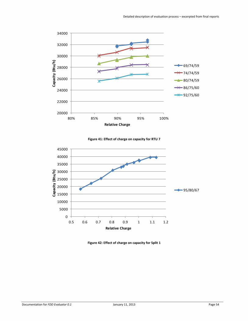
Detailed description of evaluation process – excerpted from final reports
Documentation for FDD Evaluator 0.1 January 11, 2013 Page 54
Figure 41: Effect of charge on capacity for RTU 7
Figure 42: Effect of charge on capacity for Split 1
20000
22000
24000
26000
28000
30000
32000
34000
80% 85% 90% 95% 100%
Cap
acit
y (B
tu/h
)
Relative Charge
Capacity for RTU 7
69/74/59
74/74/59
80/74/59
86/75/60
92/75/60
0
5000
10000
15000
20000
25000
30000
35000
40000
45000
0.5 0.6 0.7 0.8 0.9 1 1.1 1.2
Cap
acit
y (B
tu/h
)
Relative Charge
Capacity for Split 1
95/80/67

Detailed description of evaluation process – excerpted from final reports
Documentation for FDD Evaluator 0.1 January 11, 2013 Page 55
Figure 43: Effect of charge on capacity for Split 3
Figure 44: Effect of charge on capacity for Split 4
28000
29000
30000
31000
32000
33000
34000
35000
36000
37000
38000
0.7 0.8 0.9 1 1.1 1.2
Cap
acit
y (B
tu/h
)
Relative Charge
82/80/56
95/80/67
82/80/67
20000
22000
24000
26000
28000
30000
32000
34000
36000
38000
40000
70.00% 80.00% 90.00% 100.00%110.00%120.00%130.00%
Cap
acit
y (B
tu/h
)
Relative Charge
Capacity for Split 4
95/80/67
82/80/67
82/80/56
125/80/56

Detailed description of evaluation process – excerpted from final reports
Documentation for FDD Evaluator 0.1 January 11, 2013 Page 56
Figure 45: Effect of charge on capacity for Split 5
20000
22000
24000
26000
28000
30000
32000
34000
36000
38000
40000
0.7 0.8 0.9 1 1.1 1.2 1.3
Cap
acit
y (B
tu/h
)
Relative Charge
Capacity for Split 5
95/80/67
82/80/56
82/80/67
125/80/57


