AC 2009-2295: EXCEL IN ME: EXTENDING AND REFINING UBIQUITOUSSOFTWARE TOOLS
Kenny Mahan, University of Alabama
Jesse Huguet, University of Alabama
Joseph Chappell, University of Alabama
Keith Woodbury, University of Alabama
Robert Taylor, University of Alabama
© American Society for Engineering Education, 2009
Page 14.600.1

Excel in ME: Extending and Refining Ubiquitous Software Tools
(Excel Modules for Thermodynamic Properties of Refrigerants R134a and R22 and
Compressible Ideal Gas Flow)
Abstract
Microsoft Excel is a ubiquitous software tool that provides an excellent electronic format for
engineering computation and organization of information. This paper reports on the second year
of an NSF CCLI Phase I project to implement a sequence of Excel modules for use in the
Thermal Mechanical Engineering Curriculum.
A collection of Excel Add-ins has been developed for use in solving thermodynamics problems.
This paper reports on development of three Add-ins to compute properties of refrigerants R134
and R22 and to compute gas dynamics relations for isentropic, Fanno, and Rayleigh flows of
ideal gases. All of the Excel Add-ins developed can be downloaded at the project website
www.me.ua.edu/ExcelinME.
Intro
Under a National Science Foundation (NSF) Curriculum, Classroom, and Laboratory
Improvement (CCLI) grant a number of software modules have been developed to facilitate
engineering analysis in a computational spreadsheet. The ubiquitous spreadsheet of choice is
Microsoft Excel.
In an earlier paper by Chappell, et al. (2008), a Microsoft Excel module called XSteam,
developed by Magnus Holmgren (Holmgren 2007), was adapted and extended to compute
thermodynamic properties of steam/water from a wide range of input properties. After the
successful implementation of these expanded steam Excel modules in the classroom, attention
was turned toward adding capability for other substances, in particular the refrigerants R134a
and R22. This paper addresses the implementation and testing process of modules to calculate
the thermodynamic properties of R134a and R22.
Another topic of interest in thermodynamics is compressible flow of ideal gases. An Excel
module has been developed to compute basic functions for this area, including isentropic flow,
normal shock, Fanno Flow, and Rayleigh Flow. This paper will also present a summary of this
development.
Page 14.600.2

R134a
Description
1,1,1,2-Tetrafluoroethane, commonly referred to as R134a, is a refrigerant primarily used in
automobile air conditioners today. The R134a module developed in this work uses Excel macros
to compute the thermodynamic properties of R134a.
Why it is needed
The development of the R134a module is an important step in expanding the type of
thermodynamic problems that can be solved in Thermal Mechanical Engineering classes within
the spreadsheet environment. The addition of the R134a module allows students to tackle
problems involving refrigerants directly in the Excel spreadsheet environment without the need
of looking up values in published tables of properties.
Source for implementation
A paper by Tillner-Roth and Baehr (1994) on a fundamental equation of state for R134a has
become a standard source for computation of thermodynamic properties of R134a. Their work
and the existing XSteam module, which was expanded and modified by Huguet, et al. (2008),
were used as a starting point to implement the R134a module. The idea was to take an approach
similar to Huguet’s to expand the R134a module beyond the basic functionality provided by
Tillner-Roth and Baehr.
The fundamental equation of state for the refrigerant offers several basic relationships and
constants which were used to develop the primary functions for the R134a module in Visual
Basic. The XSteam module was invaluable to the expansion of the R134a module since the
coding used in each module was very similar. Unfortunately the R134a paper did not provide as
many initial functions as Holmgren provided in his XSteam module. To compensate, iterative
methods were implemented to develop a comprehensive module.
Naming of functions
To remain consistent with previous modules, the same naming convention used for the XSteam
module was used for the R134a module. “The name of the functions is of the form
“var1_var2var3”, where var1 is the property to be computed, var2 is the first property passed in
the call list, and var3 is the second argument passed in the call list (Woodbury, 2008).” To
differentiate R134a functions from XSteam functions, “_R134a” was appended to the end of
each R134a function name. For example, p_vT_R134a returns the pressure of R134a as a
function of specific volume and temperature.
Units
Each R134a function computes in SI units. However, if a user desires values in the US
Customary system of units, an optional third parameter is passed to the function. If the third
parameter is the character string “ENG,” then the input and output units will be US Customary
units (Woodbury, 2008).
Page 14.600.3

Implementation
For the implementation of the R134a module, fundamental correlations from Tillner-Roth and
Baehr (1994) were first used to create a set of primary functions and additional functions were
added using iteration with these primary functions.
Using regression analysis, Tillner-Roth and Baehr (1994) determined equations for vapor
pressure, saturated liquid density, and saturated vapor densities. Their paper presents the
Helmholtz free energy equation and its derivatives in dimensionless form. From the
dimensionless free energy equation and the ideal gas law, Tillner-Roth and Baher developed
equations for pressure, internal energy, enthalpy, and entropy with respect to temperature and
specific volume. The functions developed from these equations are designated primary functions
because they are computed directly using these relations from Tillner-Roth and Baher.
Since the equations provided by Tilner-Roth and Baehr’s paper only solve the primary equations
when a single phase relation exists, it was important to insert logic checks into the coding of the
primary equations to determine if the thermodynamic state resides in the two phase region. An
example of the coding of a typical primary function, p_Tv_R134a, can be seen in Figure 1. If
the state resides in the saturated region the pressure would simply be the saturation pressure at
the corresponding temperature; otherwise the single phase relationship from the paper would be
used to solve for the pressure.
After the primary functions were coded in the R134a module, the next step was to determine
what combinations of thermodynamic properties could be classified as secondary functions. To
expand this module, iterative techniques, such as the bisection or secant methods, were used to
manipulate the primary functions to develop a set of secondary functions that rely only on the
primary functions. Because this group of functions relies only on the primary functions,
additional iterations (iterations of iterations) are avoided, which help minimize the execution
time.
The bisection method was used for the iterations and an example of how it is used in the coding
of secondary functions can be seen in Figure 2. As in the coding of v_Tu_R134a, when the
thermodynamic state lies outside of the saturation region, the bisection method is implemented.
The secant method was also considered, but the bisection method was determined to be the most
robust and was utilized in all of the secondary modules.
After the possibilities of secondary functions were exhausted, the next step was to define a set of
tertiary functions that call upon both primary and secondary functions. Since tertiary functions
iterate using secondary functions that already use iterations, some of the tertiary functions
required excessive execution times or were inaccurate and were therefore abandoned.
Table 1 has a listing of all the primary, secondary, and tertiary functions that were developed for
R134a.
Page 14.600.4

Figure 1. Primary Function for p_Tv_R134a
Figure 2. Bisection Method Code in v_Tu_R134a.
Page 14.600.5

Table 1. R134a Functions with RMS Error Values Primary Functions
RMS Values
Secondary Functions
RMS Values
Tertiary Functions
RMS Values
h_px_R134a 0.0005 h_sx_R134a Abandoned h_prho_R134a 0.0042
h_Tv_R134a 0.0034 h_vx_R134a Abandoned h_ps_R134a 0.0139
h_Tx_R134a 0.0004 p_Th_R134a 0.0628 h_pT_R134a 0.0005
hL_p_R134a 0.0006 p_Ts_R134a 0.0568 p_sv_R134a Abandoned
hL_T_R134a 0.0001 p_Tu_R134a 0.0675 s_hv_R134a 0.0067
hV_p_R134a 0.0006 s_vx_R134a Abandoned s_ph_R134a 0.0068
hV_T_R134a 0.0006 T_hv_R134a 0.0015 s_pT_R134a 0.0003
p_Tv_R134a 1.2879 T_ph_R134a 0.0413 s_pv_R134a 0.0034
psat_T_R134a 0.0062 T_ps_R134a 0.0737 s_Th_R134a 0.0030
s_px_R134a 0.0005 T_pv_R134a 0.0092 s_Tu_R134a 0.0031
s_Tv_R134a 0.0032 Tsat_p_R134a 0.0005 T_hs_R134a Abandoned
s_Tx_R134a 0.0004 u_sx_R134a Abandoned T_sv_R134a Abandoned
sL_p_R134a 0.0006 u_vx_R134a Abandoned T_uv_R134a Abandoned
sL_T_R134a 0.0001 v_ps_R134a 3.7992 u_hv_R134a 0.0069
sV_p_R134a 0.0006 v_pT_R134a 0.0017 u_ph_R134a 0.0069
sV_T_R134a 0.0006 v_Th_R134a 0.0956 u_ps_R134a 0.0131
u_px_R134a 0.0005 v_Ts_R134a 0.0135 u_pT_R134a 0.0005
u_Tv_R134a 0.0033 v_Tu_R134a 0.0451 u_pv_R134a 0.0042
u_Tx_R134a 0.0003 v_sx_R134a Abandoned u_Th_R134a 0.0006
uL_p_R134a 0.0006 h_pv_R134a 0.0042
uL_T_R134a 0.0001 u_Ts_R134a 0.0026
uV_p_R134a 0.0005 u_hs_R134a Abandoned
uV_T_R134a 0.0005 u_sv_R134a Abandoned
v_px_R134a 0.0065 v_ph_R134a 3.5783
v_Tx_R134a 0.0093 h_Ts_R134a 0.0026
vL_p_R134a 0.0002 h_Tu_R134a 0.0007
vL_T_R134a 0.0003 v_hs_R134a Abandoned
vV_p_R134a 0.0083 x_hv_R134a 0.0125
vV_T_R134a 0.0115 x_hs_R134a Abandoned
x_ph_R134a 0.0106 x_sv_R134a Abandoned
x_ps_R134a 0.0113 h_sv_R134a Abandoned
x_pu_R134a 0.0118 p_hv_R134a 0.0042
x_pv_R134a 0.0065 p_hs_R134a Abandoned
x_Th_R134a 0.0278
x_Ts_R134a 0.0062
x_Tu_R134a 0.0068
x_Tv_R134a 0.0082
rhoL_T_R134a 0.0003
rhoV_T_R134a 0.0119
Page 14.600.6
Comment on Use of Thermodynamic Equation of State
One might ask why the thermodynamic equation of state (the Helmholtz function) was used as
the basis for the computation of thermodynamic properties. Why not, instead, use a table lookup
procedure such as is employed by students to solve problems? That is, why not implement the
tables within VBA as a matrix of numbers and develop algorithms based on linear interpolation
of these matrices?
The primary reason is that thermodynamic properties listed in tables in textbooks are computed
from an equation of state. This is in fact how thermodynamic properties are determined. The
most accurate method to reproduce these table values will be to use such an equation of state.
A second reason is to minimize data entry errors and reduce the need for comprehensive
verification testing. If the table of numbers from a printed set of tables were to be entered,
approximately 1,850 separate values would be needed. Each of these would need to be typed in
and verified. Also, in the verification stage, each and every pair of possible interpolation pairs
would need to be tested in order to assure accuracy. With the thermodynamic equation of state, a
random sample of points in the state space will suffice to verify the accuracy of the
implementation.
A final reason also relates to the accuracy of linear interpolation in the tables. Although printed
thermodynamic tables are touted as reliably accurate under linear interpolation, this might not
hold in the case of double or triple interpolations required for iteration of tertiary functions.
Verification of Functions
Methods for testing
To test the accuracy of the functions of the R134a module, an array of states was chosen in the
saturation, super heated, and super critical regions to generally encompass all of the
thermodynamic state space. The reference values of the properties for these states were found
from the ASHRAE R134a tables (ASHRAE, 2005). Using these fully defined states, the R134a
functions could be checked by inputting table values into pre-developed testing tables. An
example of the testing tables used to check the R134a function p_hv_R134a can be seen in
Figure 3 below.
Similar table formats where used for all function checks. Table values were manually input into
appropriate cells in the tables. To test the functions, the function in question would call upon the
input property values in the same row to compute the answer for the desired output property. To
verify the functional accuracy of the module a procedure similar to the one used by Chappel et
al. (2008) was used to check each function. The function output was compared to the table
values to check the relative error of the function at a specific state. The relative error was
calculated using Equation 1. Page 14.600.7

i
i
rel
data
datai ey
yyerror =×
−= %100% (1)
The function p_hv_R134a worked very well inside the paper’s specified temperature range of
170K (-103C) to 455K (182C) (Figure 3). When the state specified is outside of this range, the
function is programmed to return #VALUE to signal that this combination is not possible. The
goal for all functions was to have an accuracy of at most 0.5 percent error from the table values.
After the relative error was found for each of the states, an average error (RMS error) over all the
states was found for each function. Equation 2 shows how the RMS error was calculated.
n
irelRMS
n
irel
e∑== 1
2
(2)
Results of Module
Accuracy
A complete list of all primary, secondary, and tertiary functions and their RMS error values in
the R134a module can be seen in Table 1. The RMS error value represents the root mean square
error value (average relative error) for each function considering the suite of states used for
evaluation. This value indicates the average accuracy of each function when compared to the
ASHRAE table values.
As can be seen by the table, all of the RMS error values are very low except for some of the
secondary and tertiary functions that solve for or utilize specific volume. The large RMS error
values for these functions are due to table truncation errors and high sensitivity around the
saturated liquid region. The steep slope of the state space in the liquid region results in high
sensitivity to specific volume in the compressed liquid region, so even slight errors will become
greatly magnified. The table values used to verify the module’s accuracy have been truncated to
an accuracy of about four significant figures. Use of these values as data to the Excel functions
results in values that correspond to nearby states, but not exactly to the (truncated) table value.
Overall, the RMS error values of the R134a module were within the acceptable accuracy range
and well below the targeted 0.5%. The module consists of seventy-four total functions.
Computational Speed
To maintain relatively fast calculations, minimizing the number of iterations required by each
function was important. When iterative functions iterate using other iterative functions, the
speed of the calculations suffers. Steps were taken to reduce calculation time by eliminating
unneeded iterations in functions. Although the original goal was to include all available
combinations, some of the secondary and tertiary functions were abandoned due to
Page 14.600.8

Figure 3. Testing Table for a R134a function to find the pressure when enthalpy and specific
volume are known.
inconsistencies in the data and the large amount of calculation time required. The
thermodynamic combinations eliminated were uncommon combinations such as _hv, _vx, and
_sx. These combinations do not typically appear in practice or problems so they do not subtract
from the usability of the module.
A comprehensive evaluation of execution times of the functions was not conducted, but the
functions all return values typically within milliseconds. A random sampling of three of the
Page 14.600.9

tertiary functions was benchmarked for speed. The functions were called at least 1000 times
consecutively, and the VBA timer() function was used to infer the average time for execution
(ignoring overhead of the FOR..NEXT loop used in programming the test). The functions tested
and their average execution times are listed in Table 2 below. Note that the slowest of these
functions requires only 10 milliseconds to return a value.
Table 2. Average Execution Time of Selected Functions
Function Region Average Execution
Time (seconds)
x_hv_R134a Saturation 0.004078
s_pv_R134a Superheated 0.000292
v_ph_R134a superheated 0.010047
v_ph_R134a saturated 0.00075
R134a Example
Problem
A rigid, well-insulated tank having a volume of 0.2 m3 is filled initially with R134a vapor at a
pressure of 1 MPa and a temperature of 40C. A leak develops and refrigerant slowly escapes
until the pressure reaches 100 kPa. Determine the final temperature in the tank (C) and the
amount of mass that leaves the tank (kg).
Solution
The Excel solution is seen in the screen shot in Figure 4. Note the reporting format implemented
in the example solution in Figure 4 (Woodbury, 2008). This reporting format is very clear and
allows the student and reader to easily understand the approach and solution to the problem. The
report format uses the first column in the document as the “Name” column where students assign
each variable a name, such as T_1, to be used in Excel’s Name Manager. The second column is
where the actual calculation or given variable is input. The third column in the document is used
to denote the units of the variable. Lastly, the Excel equations used to arrive at the answer in the
second column is shown by placing an apostrophe (tic-mark) in front of the equation and inserted
into the fourth column. As evident by this example, the reporting format organizes the solution
very concisely.
Note that the function x_ps_R134a makes calculation of the final quality very simple. A
conventional approach to finding v_2 has been taken here, but it can be found directly once it is
recognized that the final state is fixed by P_2 and s_1. The final specific volume could be
computed directly from the function v_Ps_R134a instead. Page 14.600.10
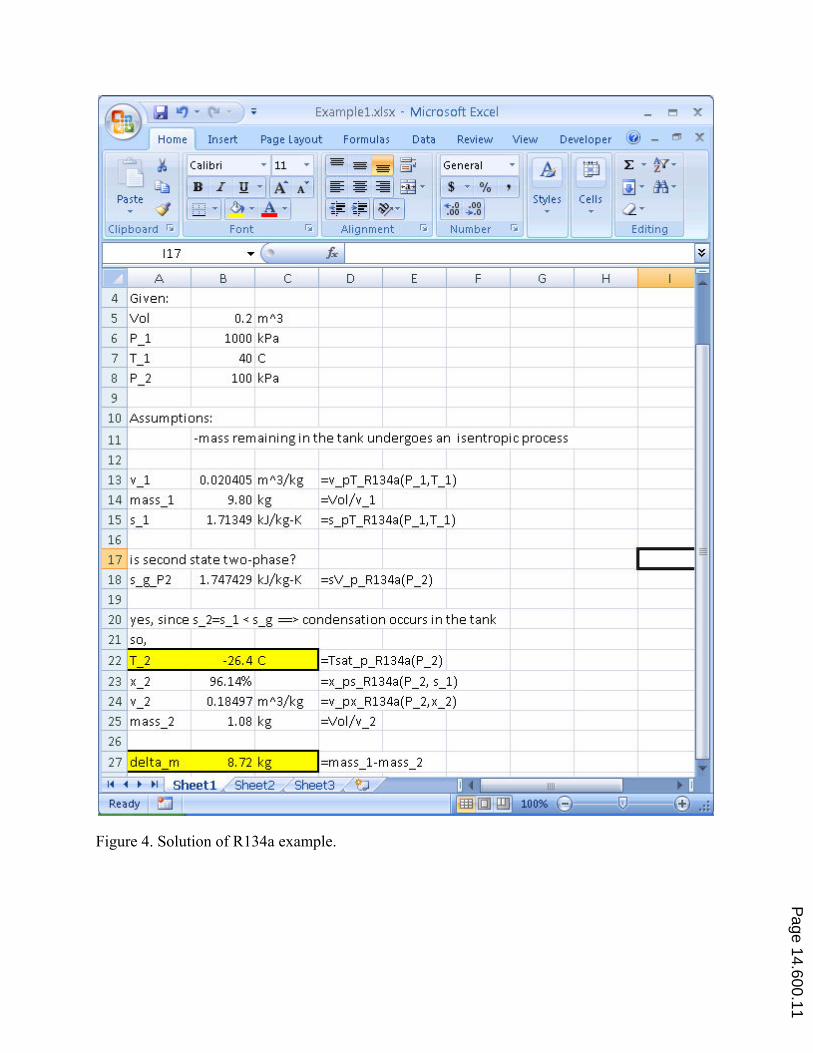
Figure 4. Solution of R134a example.
Page 14.600.11

R22
Description
Why it is needed
Although it is being phased out because of detrimental effects on the ozone layer, R22 is still
widely used as a refrigerant. As well, some thermodynamics textbooks still have problems
written for R22. Thus, it is desirable to have functions for computation of R22 properties.
During the development of the R134a module, an earlier paper giving the equation of state for
R22 was found (Wagner et al. (1993)). The structure of the equation of state for both
refrigerants R22 and R134a is very similar, so implementation of the R22 module by
modification of the R134a module was very straightforward.
Implementation
The R134a module was used as a model to code the R22 module. Each instance of _R134a
found in the R134a module was replaced with _R22 to insure a consistent naming convention.
Constants pertaining to R134a, such as critical temperature, critical density, and maximum
temperature and pressure, were replaced with the appropriate R22 properties. The only
difference in the R22 and R134a equations of state are the number of constants used and their
values. At this point, the implementation process for the R22 and R134a modules are the same
because the initial primary equations provided in the R134a and R22 papers were the same.
Evaluation of Functions
Methods for testing
For the testing of the R22 module, REFPROP (NIST, 2008) was used to determine twenty-five
random thermodynamic states from the saturation, superheated, and supercritical regions.
REFPROP 8.0 is the NIST reference fluid thermodynamic and transport properties database
which provides properties for a wide range of fluids. The process for testing the R22 module was
improved due to lessons learned from the testing of the R134a module. Instead of copying and
pasting the actual table values into each appropriate cell in the testing tables, a single table was
made of all twenty-five thermodynamic states and all their properties. As can be seen in
Figure 5, appropriate names were applied to the columns and rows of the table so that Excel’s
Name Manager could be used to assign a descriptive, dynamic name to each table value. For
example, to call the saturated vapor entropy of the first saturation state in the table “=(sat1 s_g)”
would be typed in the testing tables. By using dynamic names in the testing tables, instead of
copying and pasting all table values into hundreds of locations in the testing tables, the
possibility of data entry error was substantially minimized. This new testing technique
drastically decreased the testing time of the R22 module. Also since the table values from
REFPROP were only entered in one location, correcting possible data entry errors or checking
additional states became a very simple process. Once again a goal of only 0.5 percent error in
R22 functions was set for all functions.
Page 14.600.12

Figure 5. R22 Functions Checks Table from RefProp
Page 14.600.13

During testing, attention was given to making additional changes in the R22 code to reduce the
run time of the functions and to increase the uniformity of the module. Some of the reasons to
have unnecessarily long run times could be due to superfluous iterations and functions calls. The
first action taken to increase the speed of each calculation was to reduce the coded steps found in
the derivative equations of the Helmholtz Free Energy equations that are called by almost every
function in the module. Tau, defined as the critical temperature divided by the temperature of
the state, and Delta, defined as the density of the state divided by the critical density, were
calculated an excessive number of times within each derivative equation. Private functions were
introduced to calculate Tau and Delta and were inserted before iterations began in the derivative
functions to reduce the runtime of the functions and to make the module more uniform. All
improvements made to the R22 module to reduce calculation time and to improve uniformity
were also made in the R134a module so that consistency would exist between all modules.
Results of Module
A complete list of all primary, secondary, and tertiary functions and their RMS error values in
the R22 module can be seen in Table 3. The RMS error value represents the root mean square
error value for each function. This value shows the accuracy of each function when compared to
the REFPROP table values. Seventy-four functions were included in the R22 module. The other
seventeen functions considered were excluded because of inconsistencies in results and
excessive runtimes.
Similar to the R134a module, the results of the R22 module were very accurate. Almost all
functions fell within the desired 0.5 percent error criteria for accuracy. The RMS error values
were all reasonable except for very large error values for some of the specific volume functions.
These extreme RMS error values are highlighted in yellow in Table 3. The large error values are
due to the strong sensitivity of specific volume in the saturated liquid region.
R22 Example
Problem
Refrigerant 22 is compressed steadily from saturated liquid at 50 psia to 200 psia with an
isentropic efficiency of 88%. Determine the specific work (Btu/lbm) required. What is the
temperature of the R22 leaving the compressor?
Solution
This problem is in US Customary units so the optional argument “ENG” is given to all the
function calls to utilize these units. The solution is seen in the screen shot in Figure 6. Note that
the four-column format is adhered to, with the actual formulas used to compute the values cut-
and-pasted as visible text strings in the fourth column.
Page 14.600.14

Table 3. R22 Functions with RMS Error Values Primary RMS Secondary RMS Tertiary RMS
h_px_R22 0.0026 h_sx_R22 Abandoned h_prho_R22 0.0023
h_Tv_R22 0.0064 h_vx_R22 Abandoned h_ps_R22 0.0016
h_Tx_R22 0.0036 p_Th_R22 0.0115 h_pT_R22 0.0001
hL_p_R22 0.0043 p_Ts_R22 0.0103 h_pv_R22 0.0023
hL_T_R22 0.0061 p_Tu_R22 0.0124 h_sv_R22 Abandoned
hV_p_R22 0.0004 s_vx_R22 Abandoned h_Ts_R22 0.0016
hV_T_R22 0.0004 T_hv_R22 0.0037 h_Tu_R22 0.0003
p_Tv_R22 0.0111 T_ph_R22 0.0010 p_hs_R22 Abandoned
psat_T_R22 0.0143 T_ps_R22 0.0012 p_hv_R22 0.0190
rhoL_T_R22 0.0002 T_pv_R22 0.0014 p_sv_R22 Abandoned
rhoV_T_R22 0.0103 Tsat_p_R22 0.0007 s_hv_R22 0.0031
s_px_R22 0.0014 u_sx_R22 Abandoned s_ph_R22 0.0031
s_Tv_R22 0.0063 u_vx_R22 Abandoned s_pT_R22 0.0001
s_Tx_R22 0.0031 v_ps_R22 225.7018 s_pv_R22 0.0013
sL_p_R22 0.0023 v_pT_R22 0.0005 s_Th_R22 0.0032
sL_T_R22 0.0053 v_sx_R22 Abandoned s_Tu_R22 0.0030
sV_p_R22 0.0003 v_Th_R22 2971.1509 T_hs_R22 Abandoned
sV_T_R22 0.0005 v_Ts_R22 1437.7998 T_sv_R22 Abandoned
u_px_R22 0.0025 v_Tu_R22 0.2799 T_uv_R22 Abandoned
u_Tv_R22 0.0063 u_hs_R22 Abandoned
u_Tx_R22 0.0034 u_hv_R22 0.0002
uL_p_R22 0.0042 u_ph_R22 0.0002
uL_T_R22 0.0059 u_ps_R22 0.0014
uV_p_R22 0.0003 u_pT_R22 0.0001
uV_T_R22 0.0003 u_pv_R22 0.0022
v_px_R22 0.0026 u_sv_R22 Abandoned
v_Tx_R22 0.0086 u_Th_R22 0.0002
vL_p_R22 0.0003 u_Ts_R22 0.0015
vL_T_R22 0.0002 v_hs_R22 Abandoned
vV_p_R22 0.0032 v_ph_R22 2066.4173
vV_T_R22 0.0106 x_hs_R22 Abandoned
x_ph_R22 0.0775 x_hv_R22 0.0013
x_ps_R22 0.0623 x_sv_R22 Abandoned
x_pu_R22 0.0866
x_pv_R22 0.0031
x_Th_R22 0.0969
x_Ts_R22 0.0789
x_Tu_R22 0.1068
x_Tv_R22 0.0156
Page 14.600.15

Figure 6. Example R22 Problem.
Page 14.600.16

Gas Dynamics
Description
Algebraic equations for compressible flow of an ideal gas are quite amenable to development of
an Excel library of functions. Such a collection of functions provides an excellent substitute for
the tables of compressible flow functions in the appendix of many gas dynamics textbooks.
Availability of such a library enables engineers to perform compressible flow calculations in the
spreadsheet environment. Functions for isentropic flow, normal shock, oblique shock, Prandtl
Meyer expansion, Fanno flow, and Rayleigh flow can readily be implemented.
Implementation
Basic equations for compressible flow are readily available in most thermodynamics textbooks.
The equations used for the present development were actually taken from John and Keith (2006).
The relations were easy to code into Visual Basic for Applications (VBA) and were wrapped into
an Add-in module similar to the other suites. A list of the functions that are available in the
module is seen in Table 4.
Gas Dynamics Example
Problem
Air (γ=1.4) expands from a storage tank through a converging-diverging nozzle having a throat
area of 50 cm2. The conditions in the tank are P=200 kPa and T = 300 K. A normal shock
stands in the diverging portion of the nozzle at a location where A=100 cm2. The exit area of the
nozzle is 200 cm2. Find: a) A* from the tank to the shock location, b) A* from the shock to the
exit, c) the Mach number at the exit, d) stagnation pressure at exit, e) exit plane static pressure.
Solution
The solution to the problem is seen in the screen shots in Figures 7 and 8. Note the use of the
Excel “Goalseek” capability to do the “reverse lookup” to find the Mach number corresponding
to a known A/A* ratio in part b).
Page 14.600.17

Table 4 - Gas Dynamics Excel Add-in functions
Isentropic Suite
T_T0(M, Ȗ) static to total temperature ratio
P_P0(M, Ȗ) static to total pressure ratio
den_den0(M, Ȗ) density to density at total temperature and pressure
A_Astar(M, Ȗ) area ratio (Astar is the area corresponding to Mthroat = 1)
Rho_V(P0, T0, Ȗ, M, R) mass flux at given mach number and stagnation conditions
Standing Normal Shock Suite
SNS_M2(M1, Ȗ) mach number downstream of a normal shock.
SNS_T2_T1(M1, Ȗ) static temperature ratio across a normal shock.
SNS_P2_P1(M1, Ȗ) static pressure ratio across a normal shock.
SNS_den2_den1(M1, Ȗ) density ratio across a normal shock.
SNS_P02_P01(M1, Ȗ) stagnation pressure ratio across a normal shock.
SNS_Mexit(Pb_P01, Ae_At, Ȗ) exit mach number when a normal shock stands
Oblique Shock Suite
OBS_M2(M1, ș, Ȗ) mach number downstream of an oblique shock.
OBS_delta(M1, ș, Ȗ) turning angle in degrees –Has Units.
OBS_deltamax(M1, Ȗ) maximum turning angle in degrees
Prandtl-Meyer Function
PMF_nu(M, Ȗ) Prandtl-Meyer function Ȟ in degrees
Fanno-Flow Suite
Fan_fL_D(M1, M2, Ȗ) friction relative length.
Fan_T1_T2(M1, M2, Ȗ) static temperature ratio.
Fan_P1_P2(M1, M2, Ȗ) static pressure ratio.
Fan_P01_P02(M1, M2, Ȗ) stagnation pressure ratio.
Fan_rho1_rho2(M1, M2, Ȗ) density ratio
Rayleigh-Flow Suite
Ray_T1_T2(M1, M2, Ȗ) static temperature ratio.
Ray_P1_P2(M1, M2, Ȗ) static pressure ratio.
Ray_P01_P02(M1, M2, Ȗ) stagnation pressure ratio.
Ray_T01_T02(M1, M2, Ȗ) stagnation temperature ratio.
Ray_rho1_rho2(M1, M2, Ȗ) density ratio.
Page 14.600.18

Figure 7 – Gas Dynamics example solution part a) and b)
Page 14.600.19

Figure 8 Gas Dynamics example solution – parts c) – e)
Conclusions
With the addition of the R134a, R22 and Gas Dynamics modules, the potential use of the Excel
add-ins developed under the NSF project “Excel in ME” has been significantly expanded. The
R134a and R22 modules were developed using well-known fundamental equations of state from
the literature for each refrigerant. These equations were used to develop a set of primary
functions in Visual Basic which were then expanded by adding additional functions that iterate
using the bisection method. The R134a and R22 modules are useful to teachers and students as
they allow work in Excel without the necessity of looking up values in tables. A Gas Dynamic
module was developed using well-established algebraic relations for flow of an ideal gas. These
functions enable solution of compressible flow problems in the spreadsheet environment. All of
the Excel Add-ins developed can be downloaded at the project website
www.me.ua.edu/ExcelinME.
Page 14.600.20

Acknowledgement
This material is based upon work supported by the National Science Foundation
under Grant No. DUE-0633330. The authors gratefully acknowledge support from
this NSF award.
Disclaimer
Any opinions, findings, and conclusions or recommendations expressed in this material are those
of the author(s) and do not necessarily reflect the views of the National Science Foundation.
References
ASHRAE, (2005), Handbook of Fundamentals, http://www.ashrae.org/
Chappell, J., Taylor, R. P., and Woodbury, K. A. (2008) “Introducing Excel-based Steam Table
Calculation into Thermodynamics Curriculum,” 2008 ASEE Annual Conference &
Exposition, June 22 - 25 - Pittsburgh, PA
Holmgren, M., (2007) Excel-Engineering website. http://www.x-eng.com/
Huguet, J., Taylor, R. P., and Woodbury, K. A. (2008) “Development of Excel Add-in Modules
for Use in Themodynamics Curriculum: Steam and Ideal Gas Properties,” 2008 ASEE
Annual Conference & Exposition, June 22 - 25 - Pittsburgh, PA
John, J. E. A., and Keith, T., (2006) Gas Dynamics, Third Edition, Prentice-Hall
NIST (2008), Ref Props 8, NIST Standard Reference Database 23,
http://www.nist.gov/srd/nist23.htm
Tillner-Roth, R., and Baehr, H. D. (1994) “An International Standard Formulation for the
Thermodynamic Properties of 1,1,1,2-Tetrafluoroethane (HFC-134a) for Temperature From
170 K to 455 K and Pressures up to 70 MPa,” Journal of Physical and Chemical Reference
Data, Vol. 23, No. 5
Wagner, W., Marx, V., and Prub, A., (1993) “A new equation of state for chlorodifluoromethane
(E22) covering the entire fluid region from 116K to 550K at pressures up to 200 MPa,” Rev.
Int. Froid Vol. 16, No. 6
Woodbury, K. A., Taylor, R. P., et al. (2008) “Vertical Integration of Excel in The Thermal
Mechanical Engineering Curiculum,” 2008 ASME International Mechanical Engineering
Congress & Exposition, October 31- November 6, 2008, Boston, Massachusetts
Page 14.600.21


