
Error Component models
Ric ScarpaPrepared for the Choice Modelling Workshop
1st and 2nd of MayBrisbane Powerhouse,
New FarmBrisbane

Presentation structure
• The basic MNL model
• Types of Heteroskedasticy in logit models
• Structure of error components
• Estimation
• Applications in env. economics– Flexible substitution patterns– Choice modeling
• Future perspectives (debate)
ML – RUM Specification
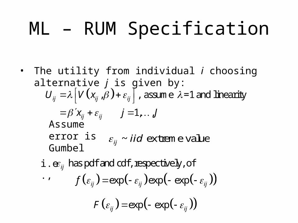
• The utility from individual i choosing alternative j is given by:
, , assume =1 and linearity
1, ,
ij ij ij
ij ij
U V x
x j J
Assume error is Gumbel
~ extreme valueij iid
i.e., has pdf and cdf, respectively, ofij
exp exp expij ij ijf
exp expij ijF

ML Choice Probabilities
• Given the distributional assumptions and representative agent specification, then defining
1
0 otherwise
ij ik
ij
U U k jy
we have that:
Pr 1| ,ij ijP y x Pr | ,ij ikU U k j x
Pr | ,ik ij ij ikV V k j x
ML Choice Probabilities (cont’d)
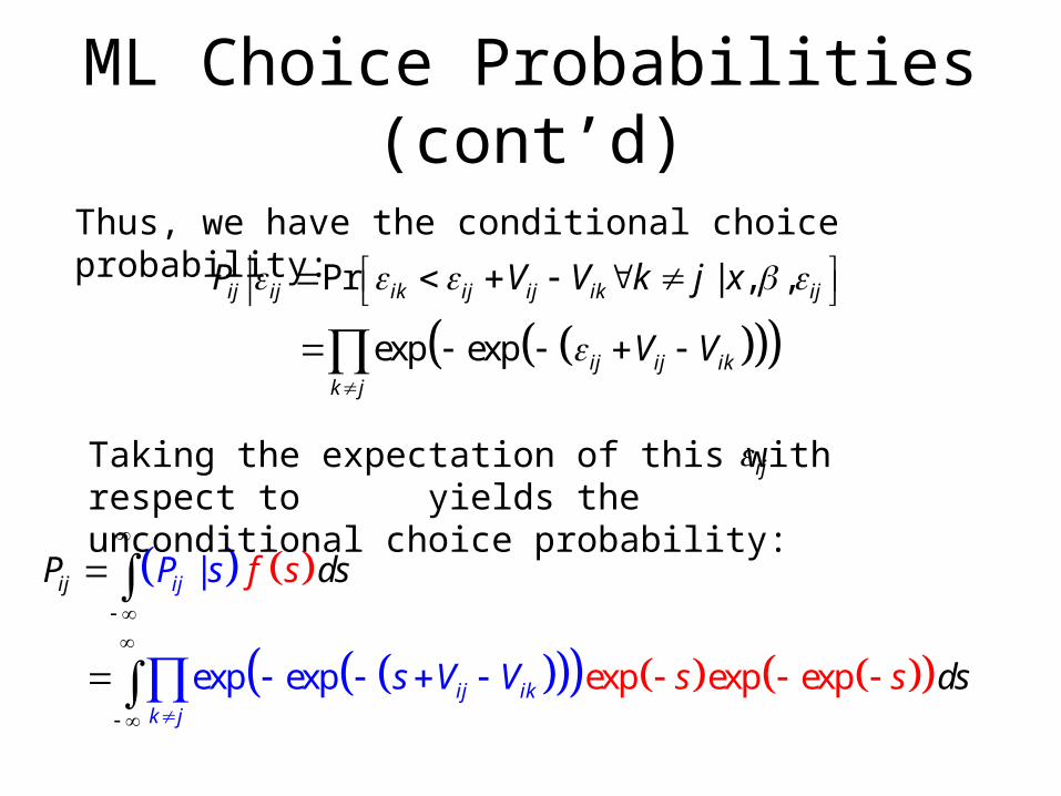
Pr | , ,ij ij ik ij ij ik ijP V V k j x
Thus, we have the conditional choice probability:
exp exp ij ij ikk j
V V
|jij iP sP dsf s
exp exp expexp exp ij ikk j
s V dV ss s
Taking the expectation of this with respect to yields the unconditional choice probability:
ij
ML Choice Probabilities (cont’d)
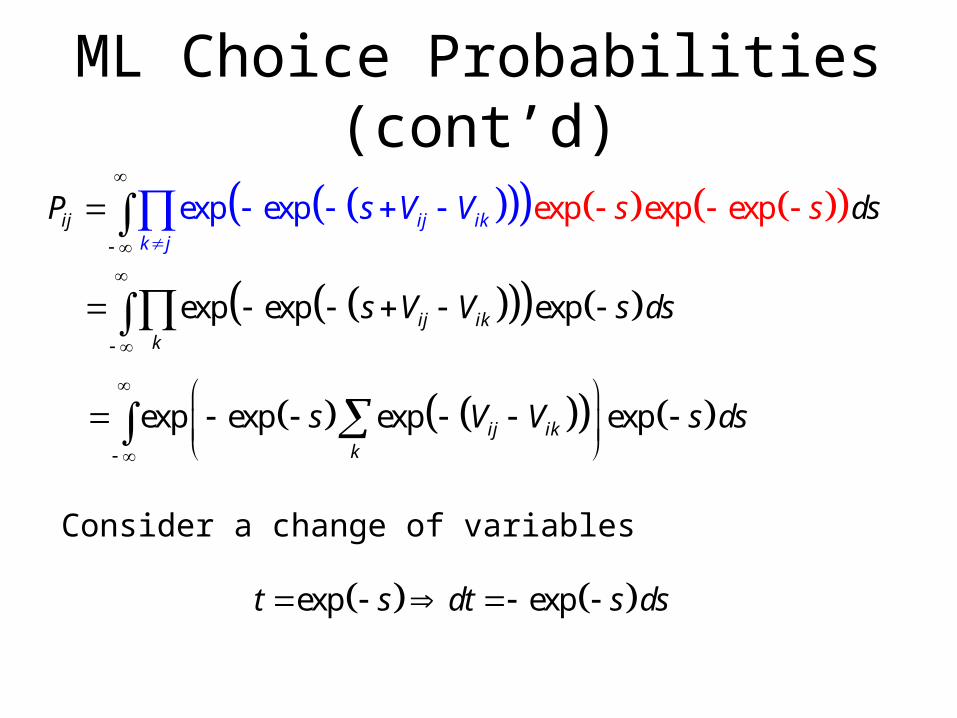
exexp exp p exp expij ikk j
ijP dsV ss sV
exp exp expij ikk
s V V s ds
exp exp exp expij ikk
s V V s ds
Consider a change of variables
exp expt s dt s ds

ML Choice Probabilities (cont’d)
exp exxp pe expij ij ikk
P V V s ss d
0
exp exp ij ikk
dtV Vt
0
exp exp
exp
ij ikj
ij ikk
V
V
t V
V
0
exp exp ij ikk
dtV Vt
1
exp ij ikk
V V
exp
expij
ikk
V
V

Merits of ML Specification
• The log-likelihood model is globally concave in its parameters (McFadden, 1973)
• Choice probabilities lie strictly within the unit interval and sum to one
• The log-likelihood function has a relatively simple form
1 1
1 1
, ln
ln exp
n J
ij iji j
n J
ij ij iki j k
L y x y P
y V V

Utility Variance in ML Specifications
• Assumes that the unobserved sources of heterogeneity are independently and identically distributed across individuals and alternatives; i.e.,
2
| , , | , ,i iVar U X Var X
I
where and 1, ,i i iJU U U
22
26
• Dependent on , but basically homoskedastic in most applications
• This is a problem as it leads to biased estimates if variance of utilities actually varies in real life, which is likely phenomenon
• Because the effect is multiplicative bias is likely to be big

Scale heteroskedasticy
…or Gumbel error heteroskedasticity• SP/RP joint response analysis allowed for
minimal heteroskedasticty (variance switch from SP to RP): i=exp(×1i(RP))
• Choice complexity work introduced i=exp(’zi), where zi is measure of complexity of choice context i
• Respondent cognitive effort: n=exp(’sn), where sn is a measure of cognitive ability of respondent n

Scale Het. limitations
• While scale heteroskedasticity allows the treatment of heteroskedasticity in the choice-respondent context it does not allow heteroskedasticity across utilities in the same choice context
• People may inherently associate more utility variance with less familiar alternatives (e.g. unknown destinations, hypothetical alternatives) than with better known ones (e.g. frequently attended sites, status quo option)
Mixed logit
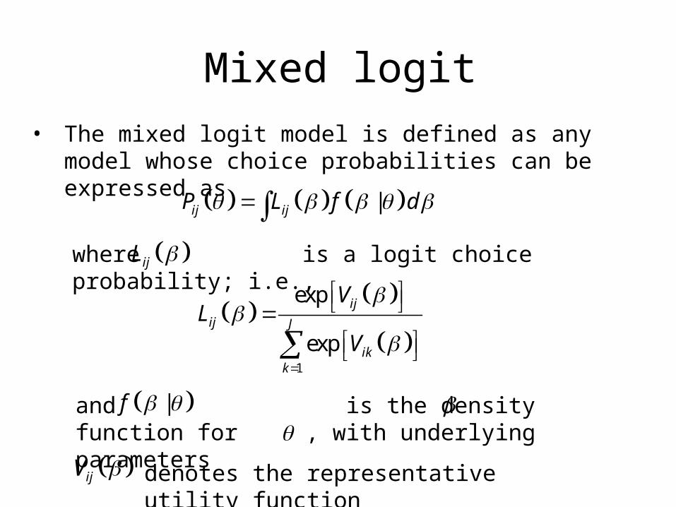
• The mixed logit model is defined as any model whose choice probabilities can be expressed as
|ij ijP L f d where is a logit choice probability; i.e., ijL
1
exp
exp
ij
ij J
ikk
VL
V
and is the density function for , with underlying parameters
|f
ijV denotes the representative utility function
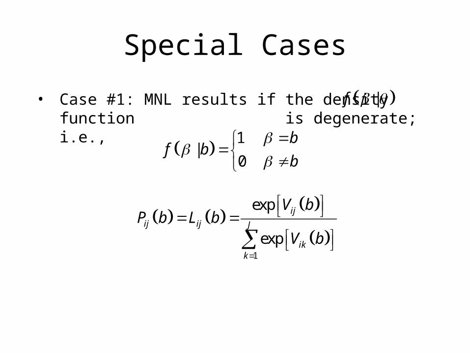
Special Cases
• Case #1: MNL results if the density function is degenerate; i.e.,
|f
1|
0
bf b
b
1
exp
exp
ij
ij ij J
ikk
V bP b L b
V b
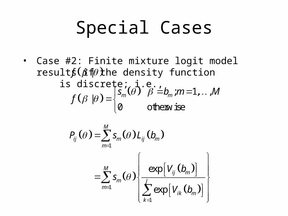
Special Cases
• Case #2: Finite mixture logit model results if the density function is discrete; i.e., |f
; 1, ,|
0 otherwisem ms b m M
f
1
1
1
exp
exp
M
ij m ij mm
Mij m
m Jm
ik mk
P s L b
V bs
V b
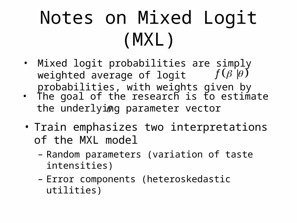
Notes on Mixed Logit (MXL)
• Train emphasizes two interpretations of the MXL model– Random parameters (variation of taste intensities)
– Error components (heteroskedastic utilities)
• Mixed logit probabilities are simply weighted average of logit probabilities, with weights given by |f
• The goal of the research is to estimate the underlying parameter vector
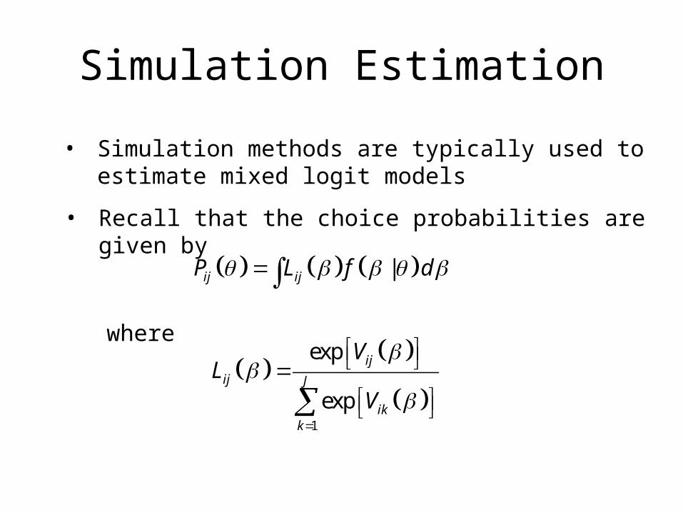
Simulation Estimation
• Simulation methods are typically used to estimate mixed logit models
• Recall that the choice probabilities are given by
|ij ijP L f d
where
1
exp
exp
ij
ij J
ikk
VL
V
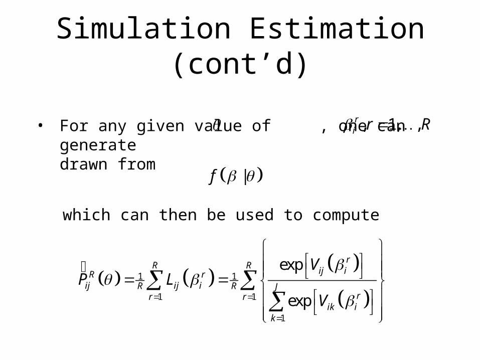
Simulation Estimation(cont’d)
which can then be used to compute
1 1
1 1
1
exp
exp
rR R
ij iR rij ij iR R J
rr rik i
k
VP L
V
• For any given value of , one can generatedrawn from
, 1, ,ri r R
|f

Simulation Estimation
1
lnN
Rij
i
L P
• The simulated log-likelihood for the panel of t choices becomes:
1
1 1 1
1
expln
exp
rN R
ijt i
R Jri r t
ikt ik
V
V
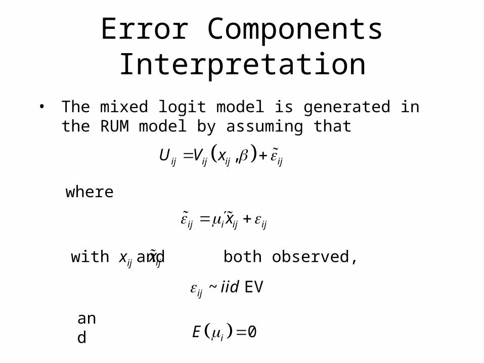
Error Components Interpretation
• The mixed logit model is generated in the RUM model by assuming that
,ij ij ij ijU V x
where
ij i ij ijx
with xij and both observed, ijx
~ EVij iid
and 0iE

Error Components Interpretation(cont’d)
• The error components perspective views the additional random terms as tools for inducing specific patterns of correlation across alternatives.
,ij ik i ij ij i ik ik
ij ik
Cov U U E z z
z z
where
ijVar

Example – Mimicking NL
• Consider a nesting structure
Stay at home (j=0)
Take a trip
Nest A Nest B
1 2 3 4
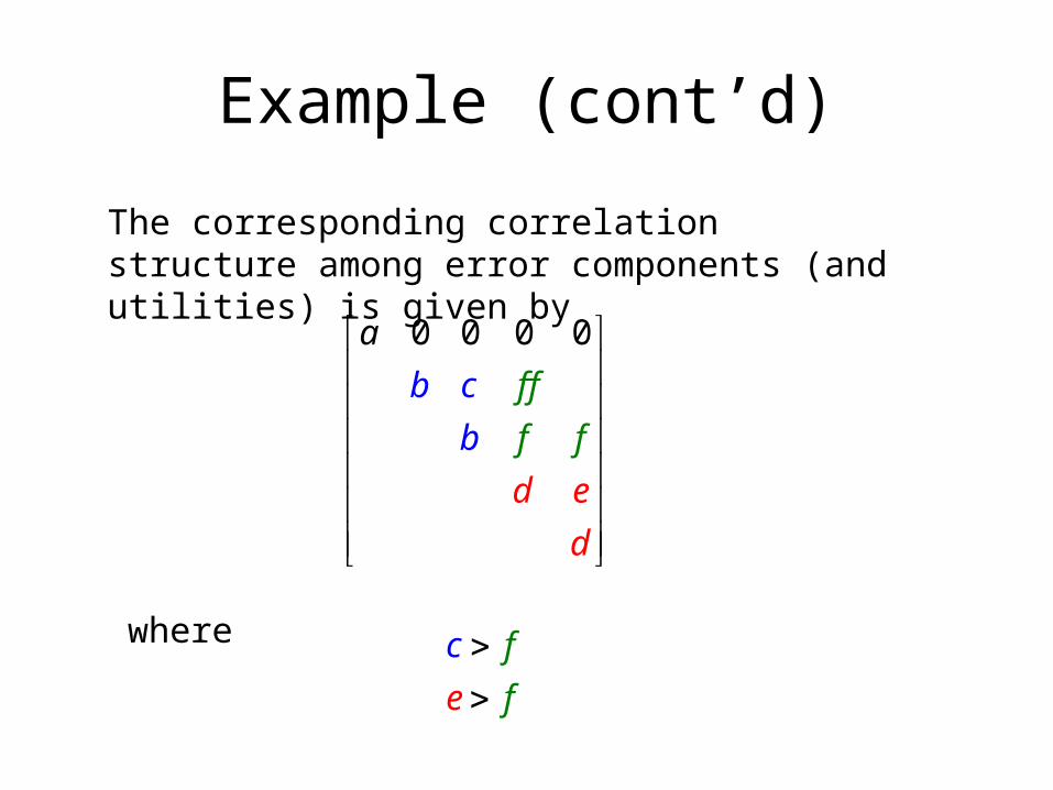
Example (cont’d)
The corresponding correlation structure among error components (and utilities) is given by
0 0 0 0
f f
f
a
b c
b f
d e
d
where c f
fe

Example (cont’d)
• We can build up this covariance structure using error components
0
1,2
3,4
ij ij
ij ij ij
ij ij
x j
U x j
x j
with~ EVij iid
i
i
2~ 0,i N
12i
12 21,2~ 0,i N
34i
34 23,4~ 0,i N

Example (cont’d)
• The resulting covariance structure becomes
2 2 2 2
2 2 2
2 21,2 1,2
21,
2
2
2
2
2
2 22 21,2 1,2
21,
22
2
0 0 0 0
ijVar U

Example (cont’d)
• One limitation of the NL model is that one has to fix the nesting structure
• MXL can be used to create overlapping nests
0 0
1 1
2 2
3 3
4 4
i i
i i
ij i i
i i
i i
x
x
U x
x
x
i
i
i
i
12i12i
34i
34i
13i
13i
14i
14i23i23i
24i
24i

Herriges and Phaneuf (2002)Covariance Pattern
1.88 2.14
-- 1.30
-- 0.64
1.61 1.09
-- 0.93
-- 0.58
1.61
-- 1.72
-- 0.08
-- 0.46
-- 0.35
-- 0.56
(1,2)(1,3)(1,4)
(1,5)( 2,3)
( 2,3,5)( 2,4)( 2,5)(3,4)(3,5)( 4,5)

Implications for Elasticity Patterns
• In general, elasticities given by
s
s
s
j ij ikjk ij
ik j ij
P x xx
x P X
,s
s
ij ij ik
ik j ij
L x f d x
x P x
,
s
ij ij ik
ik j ij
L X xf d
x P x
, , ,Lj ij jk ijw x x f d
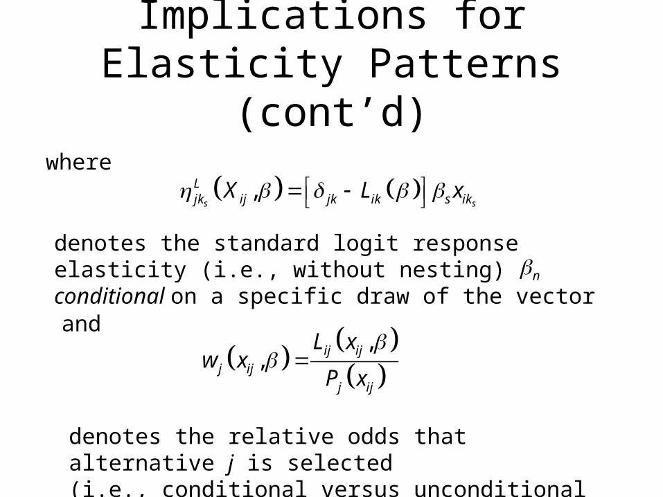
Implications for Elasticity Patterns(cont’d)
where
,s s
Ljk ij jk ik s ikX L x
denotes the standard logit response elasticity (i.e., without nesting) conditional on a specific draw of the vector n
and
,,
ij ij
j ij
j ij
L xw x
P x
denotes the relative odds that alternative j is selected(i.e., conditional versus unconditional odds)

Illustration – Choice Probabilities
0.65 0.20 0.03 0.20 0.45
0.09 0.20 0.24 0.20 0.14
0i iL
; 0ij iL j
2i 0i 2i
j jP L f d
0.1 10

Choice modeling• Error component in hypothetical alternatives,
yet absent in the SQ or no alternative
The induced variance structure across utilities is:

Effect
• Fairly general result that it improves fit while requiring few additional parameters (only st. dev. of err. comp.)
• It can be decomposed by socio-economics covariates (e.g. spread of error varies across segments of respondents)

Adoption and state of practice
• Error component estimators have now been incorporated in commercial software (e.g. Nlogit 4)
• Given their properties and the flexibility they afford they are likely to be increasingly used in practice


![[Architecture ebook] Carlo Scarpa](https://cdn.vdocuments.site/doc/165x107/55cfeb0a5503467d968bd917/architecture-ebook-carlo-scarpa.jpg)


