
Wind turbines in complex terrain (NREL)
Instream MHK turbines in complex bathymetry (VP East channel NewYork)
Common features?
1) horizontal axis turbine
producing power
2) complex incoming flow
conditions (bridge pier, karman
vortices, bluff body wakes and
turbine wakes)
Energy from wind and water extracted by Horizontal Axis Turbine

First goal of a power plant: extract energy efficiently and for a long time
with minimal maintenance costs.
P = ½ cp A U3 mean power output given a mean incoming flow velocity
representative of the actual flow distribution across the rotor
of area A
Turbine lifetime
operation and
maintenance
costs
unsteady loads on the blades, low and high speed
shaft, support tower (in general, on all device’s
components)
The source of such unsteadiness comes
from the turbulence of the incoming flow.
What else ?

Second goal of a renewable energy power plant: work efficiently with a minimal environmental footprint
MHK instream turbines:
erodible sediment layer variable B.C.
short and long term impacts
on river morphodynamics and sediment transport
Wind Turbine:
wake flow, alteration
of the local heat flux,
but most of it:
noise, bats and birds
No noise
birds fishes
Let us consider that a renewable energy source does not
automatically imply that the power plant is
environmentally sustainable

Buck and Renne 1985: wake effect on full-scale 2.5 MW turbines
• Presented summary of turbine/turbine (power deficit) and turbine/met tower
wake interactions (velocity deficit from freestream tower to wake tower)
• Examined wake changes due to thermal stability, wind speed, and
turbulence
Source: Buck, Renne
1985
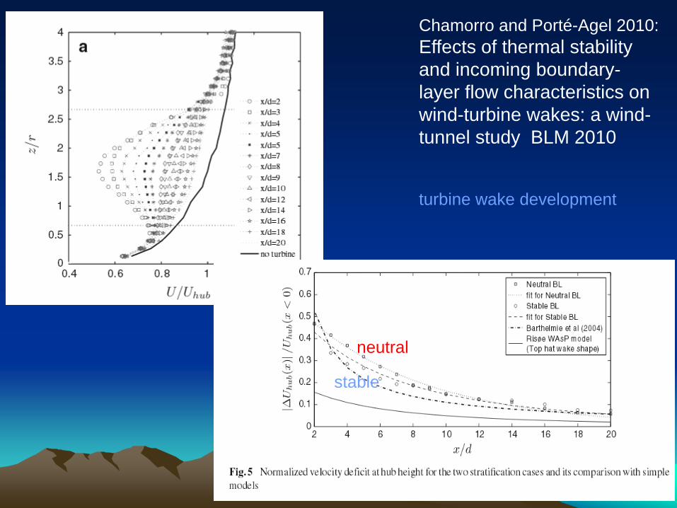
Chamorro and Porté-Agel 2010:
Effects of thermal stability
and incoming boundary-
layer flow characteristics on
wind-turbine wakes: a wind-
tunnel study BLM 2010
turbine wake development
neutral
stable

Raul Cal 2010, the problem of double averaging equation for modeling turbine wake
Entrainment of high momentum fluid
into the wind power plant is due to
turbulence at the “canopy” interface

– Chamorro and Porté-Agel 2010 – Effects of thermal stability and
incoming boundary-layer flow characteristics on wind-turbine
wakes: a wind-tunnel study
neutral
stable

• Turbine wake research (miniature turbines)
– Zhang, Markfort, Porté-Agel 2012 – Near-wake flow structure
downwind of a wind turbine in a turbulent boundary layer
• PIV and hot-wire anemometer
blade
wake

Main ingredients in the wake:
tip and hub vortices, vortex sheets
wake shear layers
wake expansion
wake deficit
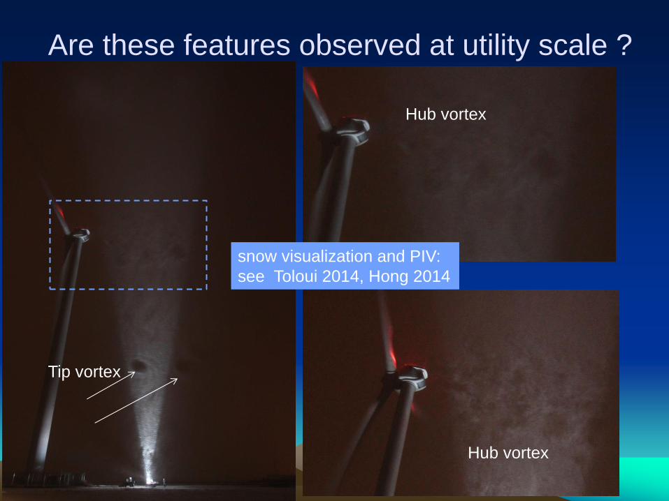
Are these features observed at utility scale ?
Tip vortex
Hub vortex
Hub vortex
snow visualization and PIV:
see Toloui 2014, Hong 2014
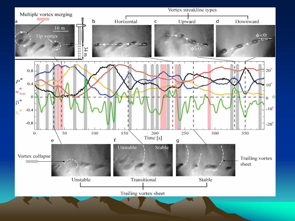
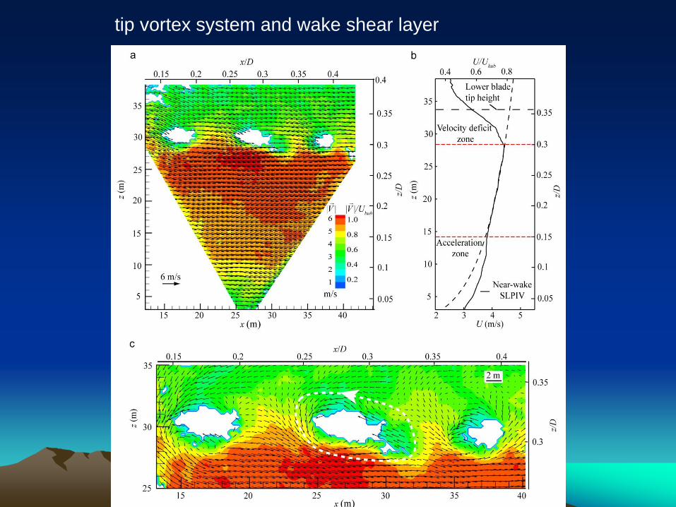
tip vortex system and wake shear layer
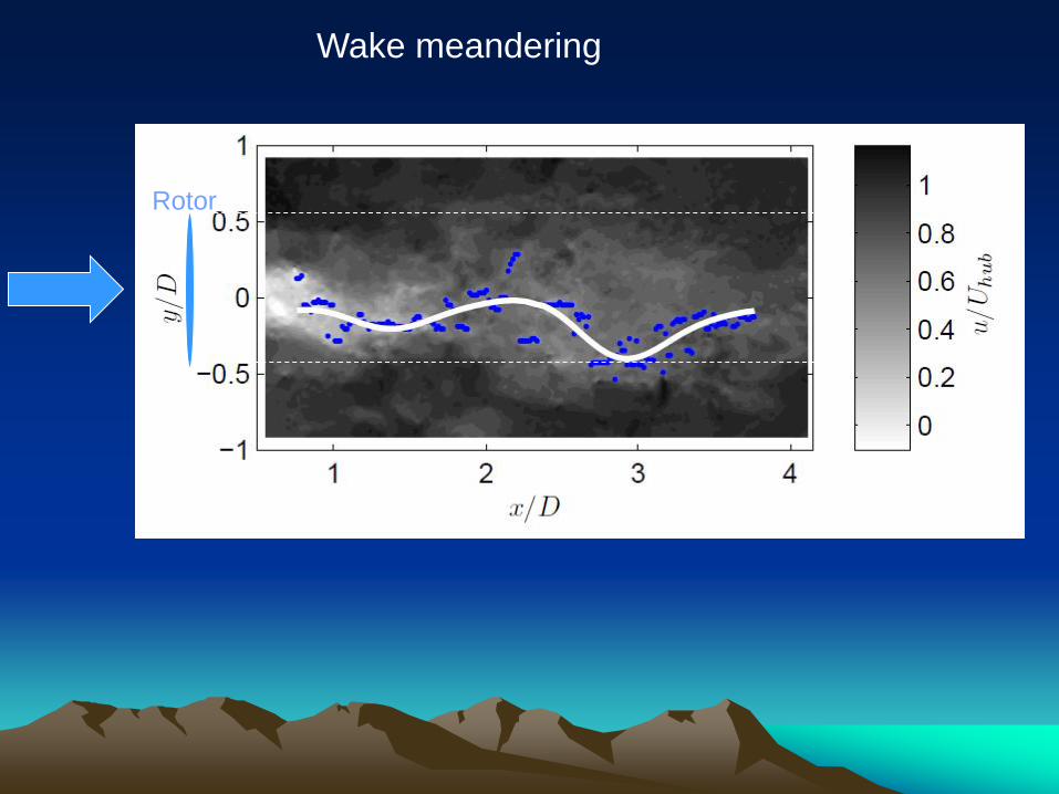
Rotor
Wake meandering

Domain of low speed meander oscillation ...
Is it important ? Does it depend on turbine operating conditions?
Tip vortex
Potential
tip vortex – meander
interaction
leading to wake
instability
A,
We can define the meandering
wavelength and amplitude A , the
expansion angle of the meandering
domain and the mean velocity Uc in
the domain

Two flow meander populations have a distinct Stouhdal number
Let us consider A1 1 Uc1
St1 ~ 0.7
in the range 0.44 ∼ 0.81
explored by Viola, 2014, Iungo, 2014
recognized as the signature of the hub vortex
(Kang and Sotiropoulos 2014)
Let us consider A2 2 Uc2
St2 ~ 0.3
1 2
Medici et al. 2008 reported
values in the range of 0:15
∼ 0:25, Chamorro et
al.2013 observed a peak at
0.28 while Okulov and
Sorensen2014 estimated a
peak at 0.23, both at
x=D ≃ 5.
wake
meandering
oscillation
hub vortex
oscillation

Annoni et al WE
Near and far wake
distinction is based on
the signature of turbine
geometry on the flow
statistics.
Far wake instead has
some intrinsic instability
modes known as wake
meandering
why wake modeling is important ?

The induction factor a is defined
based on the velocity deficit “within”
the rotor plane. Why?
because u is the average velocity at
the low pressure side of the rotor. u
must be >0 so the rotor becomes a
porous disk
radial symmetry actuator disk model

The normalized thrust coefficient and power coefficient depend on
a a=1/3 corresponds to a max Cp identified by the Betz limit of 59.3%
0<a<1 implies that u>0 and u< U
no flow passing through the turbine
all flow passing through the turbine
as if the turbine does not exist

In fact a depends on
the turbine operating conditions, which are defined by the tip
speed ratio and by the pitch blade angle
where =Utip /U = R/ U
while is used to change the blade angle of attach amplifying or
reducing aerodynamic lift torque
J moment of inertia

with increasing complexity and computational costs..
actuator lines models: blade rotation is implemented,
no nacelle no hub vortex (so far...)
high resolution required
fully resolved turbine-blade geometry
very high resolution is required

What are the modeling assumptions , so far ?
1) uniform inflow
2) no turbulence
How can we make sure that the turbine is always operating at optimal conditions ?
Especially if:
the incoming flow is unsteady angle of attack is varying ...
the mean incoming flow is not uniform (boundary layer, or flow within a farm, or
complex terrain effects)
We have some options...
1) improve wake models
2) wind preview: measuring the incoming flow approaching the turbine
3) wind power plant optimization: do not operate each single turbine at optimal
conditions but optimize the full power plant Cp
Remember Cal 2010: how do we bring more high momentum fluid in the turbine
from flow layers above the top tips
increase mixing, increase power density (optimal streamwise-transverse turbine
spacing,

1) Improve (static) wake models
Realistic wake with turbine in two operating conditions (optimal-rated)
suboptimal (derated towards large low )
note that we can modify the
wake expansion angle k (Park
model), adding a dependency on
Cp
e.g. derated k=0.15, rated k=0.09
or introduce a Gaussian profile
instead of the Park “hat”
optimal
TSR
derated

2) Build a dynamic model able to account for wake meandering
(or any scale dependent incoming flow perturbation amplitude
modulation+phase shift). Question is: how can we optimize back
wind turbines base on front turbines performance or state ...
1) test how turbine response (in freq.) propagates
through the wind power plant
1) Improve (dynamic)wake models

• Experimental setup:
– Full-scale testing at Eolos, flow measurements with WindCube
LiDAR
• Inflow and wake data
• Turbine SCADA data
– Model-scale data for comparison
2) Upwind Preview
LiDAR wake
measurements
LiDAR inflow
measurements

• Methods for velocity calculation with LiDAR
– Standard WindCube N on north
– 2D (Planar) Velocity Calculation with NS aligned
with the mean wind
2) Upwind Preview

Inflow and wake Analysis: Wind tunnel - EOLOS
• LiDAR velocity profile
– 1 Hz measurement
• 1 beam per second
– Averaging volume
• Calculates u,v,w from 3 previous
measurements
• Averaging region increases w/
height
• PIV data
– To mimic LiDAR, average in x
• Averaging distance defined from
x/D
z/z h
ub
x/D
26 Howard K.B. and Guala M. AIAA conf. 2013
2) Upwind Preview

• Full Scale Velocity profile
– Profile curvature at x/D=-0.8 • EOLOS convex curve over rotor
• Blockage compared to clean flow
• Scale Comparison
– Blockage at hub height • EOLOS – ΔU/Uhub ≈ 0.053
• Model - ΔU/Uhub ≈ 0.049
– Shear change – many influences • Re #, surface roughness, etc.
27
z/z h
ub
U /Uhub
U /Uhub
z/z h
ub
2) Upwind Preview

Wake Analysis: Full- to Model-Scale Profiles
Velocity profile comparison
28
z/z h
ub
z/
z hu
b
EOLOS - LiDAR Wind Tunnel - Hotwire
1.5D 2.5D 3D
(U - Uinflow)/Uhub (U - Uinflow)/Uhub (U - Uinflow)/Uhub
(U - Uinflow)/Uhub (U - Uinflow)/Uhub
Singh et al. subm.
2) Upwind Preview

• Tracking the response of the Eolos turbine to inflow
- - – LiDAR Uhub
- - – LiDAR Utop-tip
- – Eolos power
Black dots – Root blade strain
– Power and strain
appear to track
velocity fluctuations
– Gust event details
strain response
– Turbine response
2) Upwind Preview

• Tracking the response of the Eolos turbine to inflow
– LiDAR tracking up to 8 elevations within rotor swept area
– Turbine power output, blade strain, etc.
– Each time signal velocity time signal can be correlated to turbine
data
2) Upwind Preview

• Cross-correlation – Power to inflow
– Rotor averaged time signal
• Full-scale data produces 𝜌𝑃𝑢 = 0.82
• Model-scale produces 𝜌𝑃𝑢 = 0.64
– Signal from each elevation
• Full-scale peak at z/zhub=1.3
• Model-scale peak at z/zhub=1.2
– For turbine-turbine arrangement
• First inspect turbine wake
• Peak correlation occurs at hub height
At z/zhub~1.3 corresponding to z=zhub+L/4
the wind velocity is mostly correlated with
power output and blade strain.
This signal can be thus used as a wind input
for a predictive control strategy (front
turbines). For back turbines z/zhub~1
2) Upwind Preview
Question: which control solution can we implement just due to the fact that the
turbine is in boundary layer ?

• Experimental setup: – SAFL wind tunnel (same boundary layer conditions as previous)
• Note that the ceiling was adjusted to account for blockage induced by the turbines
– Voltage acquisition from each turbine
– Wall parallel PIV (i) between rows and (ii) between columns (last row)
– Four test conditions • Aligned
• Staggered
KBH | St. Anthony Falls Lab 32
3) wind power plant optimization
• Yaw Misalignment
• TSR Adjustment

• Aligned farm, spacing effect on total production – 4% reduction from lx = 6D to 5D
– 7% reduction from lx = 6D to 4D
– 13% reduction from lx = ∞D to 6D
• Aligned vs Staggered total production – Staggered has 11.9% increase over aligned farm
with the same spacing
KBH | St. Anthony Falls Lab 33
Δ - lx = 6D - lx = 5D - lx = 4D
○
□
3) wind power plant optimization
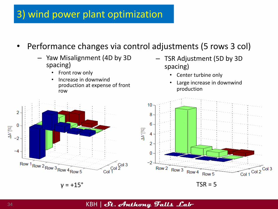
• Performance changes via control adjustments (5 rows 3 col)
KBH | St. Anthony Falls Lab 34
– Yaw Misalignment (4D by 3D spacing)
• Front row only • Increase in downwind
production at expense of front row
– TSR Adjustment (5D by 3D spacing)
• Center turbine only
• Large increase in downwind production
γ = +15° TSR = 5
3) wind power plant optimization

• Total Farm Production Change – Yaw Misalignment
• Production from 5 rows and 3 columns
– TSR Adjustment • Production from 4 rows and 3 columns
• Needs further refinement to measure production change of derated turbine
KBH | St. Anthony Falls Lab 35
3) wind power plant optimization
KBH | St. Anthony Falls Lab 36
• Summary of Findings – Aligned farm spacing
• Intuitive, larger spacing is better – 7% reduction for 6D to 4D
• optimal spacing is an economic problem, not a fluid mechanic problem
– Staggered vs aligned • Staggered 12% more production for 5 rows, 3 cols spaced at lx = 5D and ly = 3D
– Farm performance modification • Yaw misalignment
– Smallest reduction at 0.3% for farm production
• TSR adjustment
– Most effective change, from TSR 3.2 to 5 with nearly 1% increase
– Provides promising results, needs further investigation
3) wind power plant optimization
If we change the point of view and we investigate:
1) what flow structures the turbine feels ?
(unsteady loads cascading down from blades to
foundation)
2) in the TKE scale by scale budget , what survives
in the wake ?
3) What do we have to take into account in the
turbine control?

what are the relevant scales of the order (1/2, 1/3) of the rotor diameter
depending on the tip speed ratio
( on non erodible-concrete channel , Chamorro et al. 2013)
similar evidence is provided for the EOLOS wind turbine
Moving on with this talk...
What are the large scales of the flow in the atmospheric boundary layer ?

Ret = 5884
Ret = 14380
Ret = 106
Ret = 520
Ret = 106
Ret = 106
Very large
scale motion
Super-
structures
Kim & Adrian 99
Balakumar 07
Guala et al. 06, 10, 11
Hutchins et al 2007, 2013
Monty et al 2009
Mathis et al. 2009
Marusic, et al. 2011

Upwind flow perturbations
1) Turbine in baseflow
2) Two turbines in series
3) Sinusoidal hill upwind
of turbine
Simultaneous PIV measurement windows
Flow
Karman vortex shedding
DC motor voltage

𝜆 = 𝜏𝑢𝑐𝑜𝑛𝑣𝑒𝑐𝑡𝑖𝑜𝑛 𝜌𝑥𝑦(𝜏) =𝑣𝑥(𝑡)𝑣𝑦(𝑡 + 𝜏)
𝑣𝑥2 𝑣𝑦
2
T
Turbine and Turbine interactions
~6-10 consistent with VLSM (rotational inertia ?)

What is the effect of a turbine on the incoming flow ?
8<x/D<12
Premultiplied spectral
difference (f, z)
turbine wake – incoming flow
enhanced turbulence
dampened turbulence
Chamorro, Guala , Arndt & Sotiropoulos, JOT 2012
2<x/D<6
x/D near wake far wake

The rotor
diameter
d

Adding complexity: Varying thermal stability regimes
stable neutral convective
stable
convective neutral
Top tip
Bottom tip
o – Neutral □ - Stable ◊ - Convective
(Howard K.B. , Chamorro L.P., Guala M. AIAA 2012, to be submitted to BLM)

Stab
le
Co
nve
ctiv
e
U/Uhub
RESULTS: thermal stability regimes coupled with topographic effects
baseflow-neutral hill - stable
see also Singh, Howard, Guala PoF 2014

The curious case of hill-turbine in the stratified (stable) regime
NEUTRAL
Voltage spectra
The very large scales motions are deflected by the hill for all thermal regimes
neutral stable convective
ST TT
(Howard K.B. , Hu. SJ., Chamorro L.P., Guala M. Wind Energy 2014)
however, thermal stratification inhibits momentum flux in the vertical direction expanding the wake in the cross-flow direction.
thus, in the stratified regime the hill exerts a sheltering effect on the turbine


