
Impedance
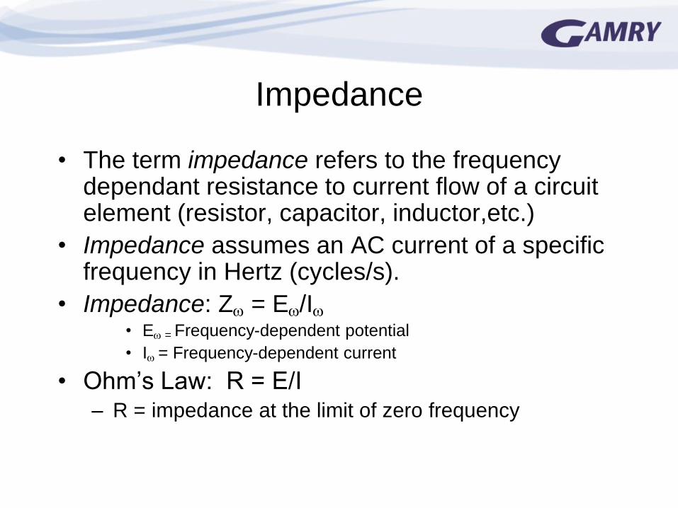
• The term impedance refers to the frequency dependant resistance to current flow of a circuit element (resistor, capacitor, inductor,etc.)
• Impedance assumes an AC current of a specific frequency in Hertz (cycles/s).
• Impedance: Z = E/I
• E = Frequency-dependent potential
• I = Frequency-dependent current
• Ohm’s Law: R = E/I – R = impedance at the limit of zero frequency
Reasons To Run EIS • EIS is theoretically complex (and can be expensive) –
why bother? – The information content of EIS is much higher than DC
techniques or single frequency measurements.
– EIS may be able to distinguish between two or more electrochemical reactions taking place.
– EIS can identify diffusion-limited reactions, e.g., diffusion through a passive film.
– EIS provides information on the capacitive behavior of the system.
– EIS can test components within an assembled device using the device’s own electrodes.
Making EIS Measurements
• Apply a small sinusoidal perturbation (potential or current) of fixed frequency
• Measure the response and compute the impedance at each frequency. – Z = E/I
• E = Frequency-dependent potential
• I = Frequency-dependent current
• Repeat for a wide range of frequencies
• Plot and analyze
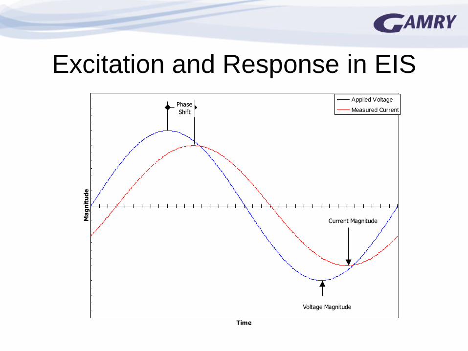
Excitation and Response in EIS
Time
Ma
gn
itu
de
Applied Voltage
Measured CurrentPhase
Shift
Voltage Magnitude
Current Magnitude
EIS Data Presentation
• EIS data may be displayed as either a vector
or a complex quantity.
• A vector is defined by the impedance
magnitude and the phase angle.
• As a complex quantity, Ztotal = Zreal + Zimag
• The vector and the complex quantity are
different representations of the impedance
and are mathematically equivalent.
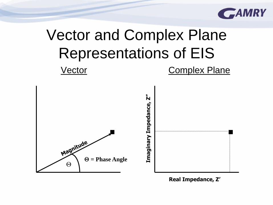
Vector and Complex Plane
Representations of EIS Vector Complex Plane
Real Impedance, Z’
Im
ag
ina
ry I
mp
ed
an
ce
, Z
”
= Phase Angle
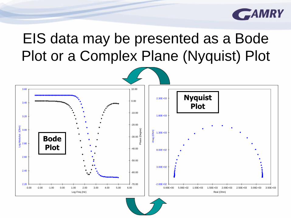
EIS data may be presented as a Bode
Plot or a Complex Plane (Nyquist) Plot
2.20
2.40
2.60
2.80
3.00
3.20
3.40
3.60
-3.00 -2.00 -1.00 0.00 1.00 2.00 3.00 4.00 5.00 6.00
Log Freq (Hz)
Log M
odulu
s
(Ohm
)
-70.00
-60.00
-50.00
-40.00
-30.00
-20.00
-10.00
0.00
10.00
Phase (
Degre
e)
-2.00E+02
3.00E+02
8.00E+02
1.30E+03
1.80E+03
2.30E+03
0.00E+00 5.00E+02 1.00E+03 1.50E+03 2.00E+03 2.50E+03 3.00E+03 3.50E+03
Real (Ohm)
-Im
ag (
Ohm
)
Bode Plot
Nyquist Plot
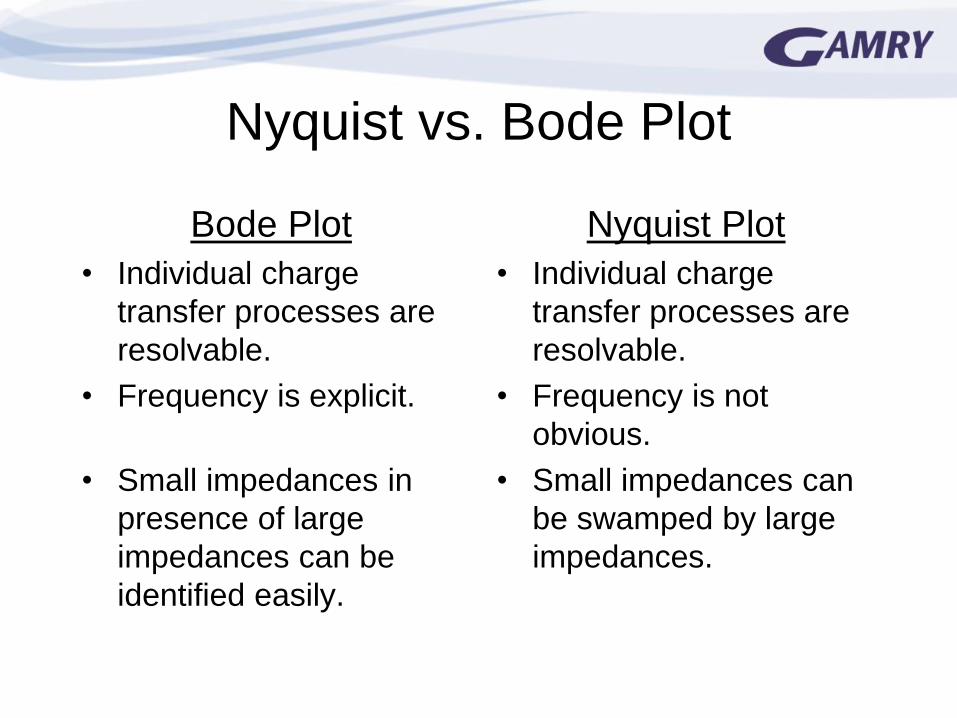
Bode Plot
• Individual charge
transfer processes are
resolvable.
• Frequency is explicit.
• Small impedances in
presence of large
impedances can be
identified easily.
Nyquist Plot
• Individual charge
transfer processes are
resolvable.
• Frequency is not
obvious.
• Small impedances can
be swamped by large
impedances.
Nyquist vs. Bode Plot
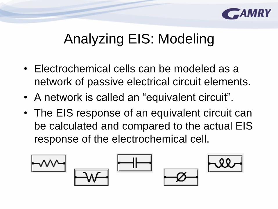
Analyzing EIS: Modeling
• Electrochemical cells can be modeled as a
network of passive electrical circuit elements.
• A network is called an “equivalent circuit”.
• The EIS response of an equivalent circuit can
be calculated and compared to the actual EIS
response of the electrochemical cell.
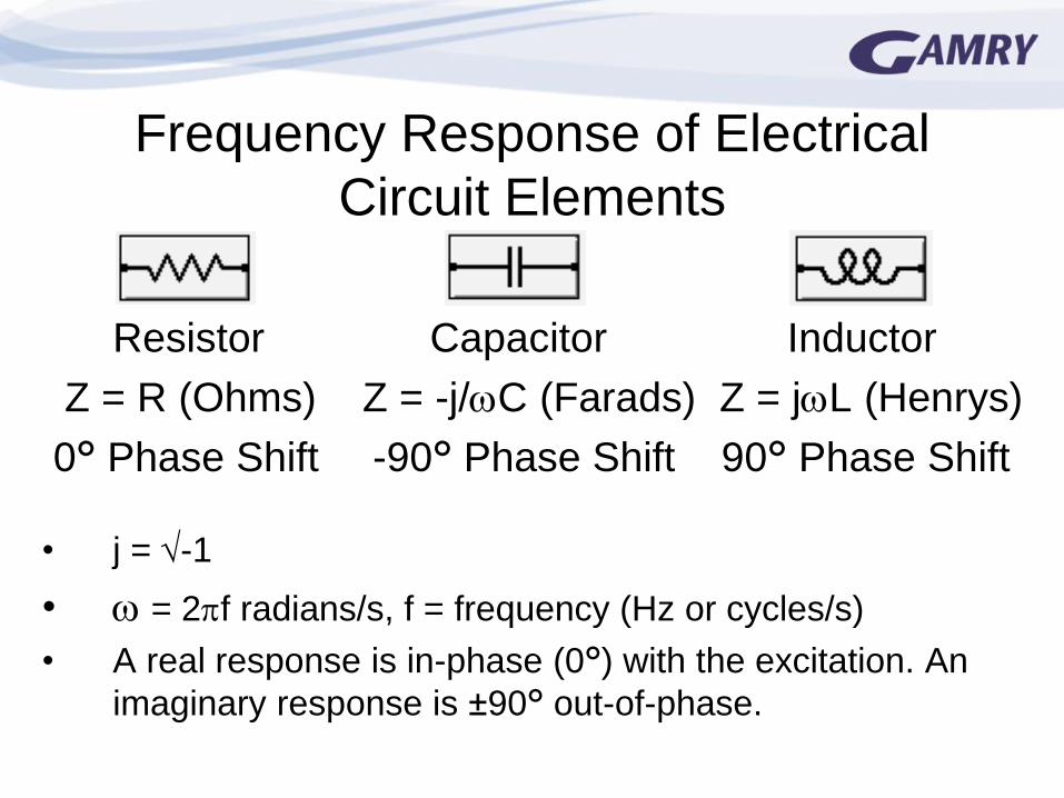
Frequency Response of Electrical
Circuit Elements
Resistor Capacitor Inductor
Z = R (Ohms) Z = -j/C (Farads) Z = jL (Henrys)
0° Phase Shift -90° Phase Shift 90° Phase Shift
• j = -1
• = 2f radians/s, f = frequency (Hz or cycles/s)
• A real response is in-phase (0°) with the excitation. An
imaginary response is ±90° out-of-phase.
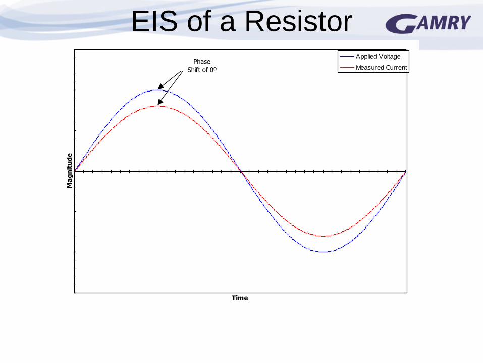
EIS of a Resistor
Time
Ma
gn
itu
de
Applied Voltage
Measured CurrentPhase
Shift of 0º
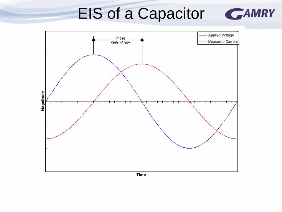
EIS of a Capacitor
Time
Ma
gn
itu
de
Applied Voltage
Measured CurrentPhase
Shift of 90º
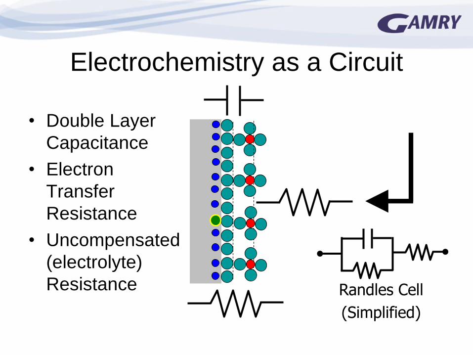
Electrochemistry as a Circuit
• Double Layer
Capacitance
• Electron
Transfer
Resistance
• Uncompensated
(electrolyte)
Resistance Randles Cell
(Simplified)

Bode Plot
2.20
2.40
2.60
2.80
3.00
3.20
3.40
3.60
-3.00 -2.00 -1.00 0.00 1.00 2.00 3.00 4.00 5.00 6.00
Log Freq (Hz)
Log M
odulu
s
(Ohm
)
-70.00
-60.00
-50.00
-40.00
-30.00
-20.00
-10.00
0.00
10.00
Phase (
Degre
e)
Phase Angle
Impedance
Ru
Ru + Rp
RU
RP
CDL
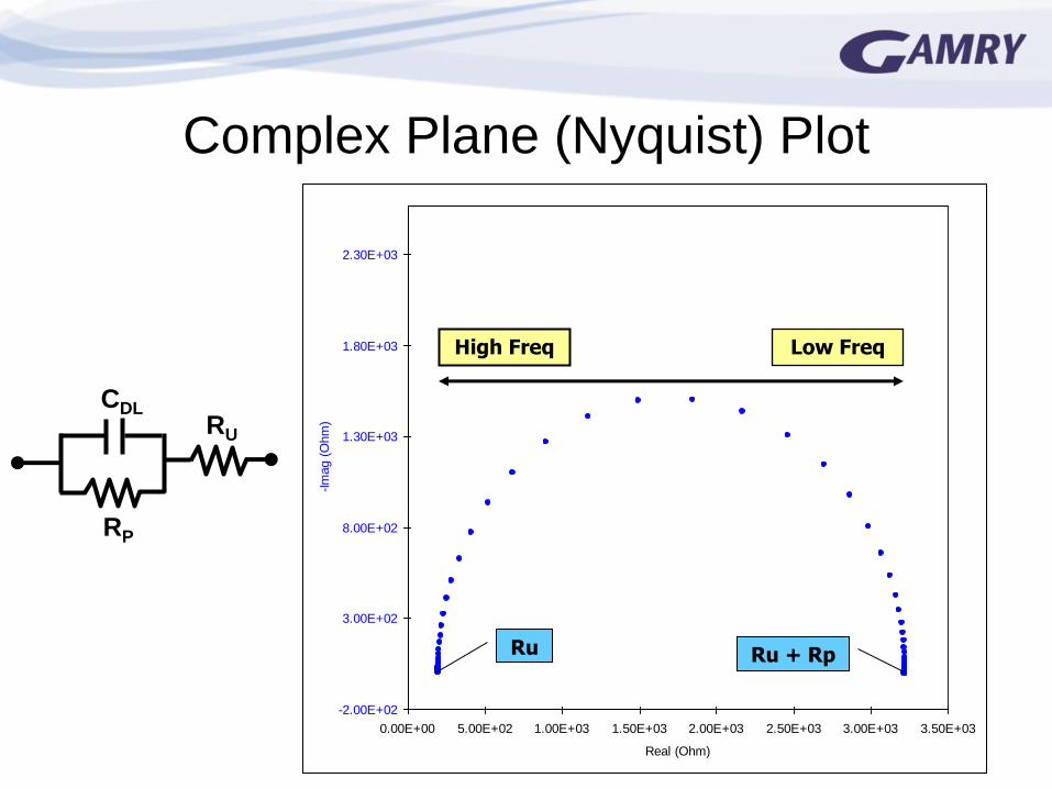
Complex Plane (Nyquist) Plot
-2.00E+02
3.00E+02
8.00E+02
1.30E+03
1.80E+03
2.30E+03
0.00E+00 5.00E+02 1.00E+03 1.50E+03 2.00E+03 2.50E+03 3.00E+03 3.50E+03
Real (Ohm)
-Im
ag (
Ohm
)
Ru Ru + Rp
High Freq Low Freq
RU
RP
CDL

Nyquist Plot with Fit
-2.00E+02
3.00E+02
8.00E+02
1.30E+03
1.80E+03
2.30E+03
0.00E+00 5.00E+02 1.00E+03 1.50E+03 2.00E+03 2.50E+03 3.00E+03 3.50E+03
Real (Ohm)
-Im
ag (
Ohm
)
Results
Rp = 3.019E+03 ± 1.2E+01
Ru = 1.995E+02 ± 1.1E+00
Cdl = 9.61E-07 ± 7E-09
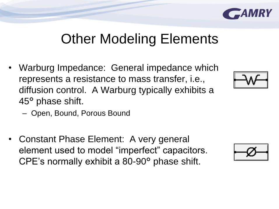
Other Modeling Elements
• Warburg Impedance: General impedance which
represents a resistance to mass transfer, i.e.,
diffusion control. A Warburg typically exhibits a
45° phase shift.
– Open, Bound, Porous Bound
• Constant Phase Element: A very general
element used to model “imperfect” capacitors.
CPE’s normally exhibit a 80-90° phase shift.
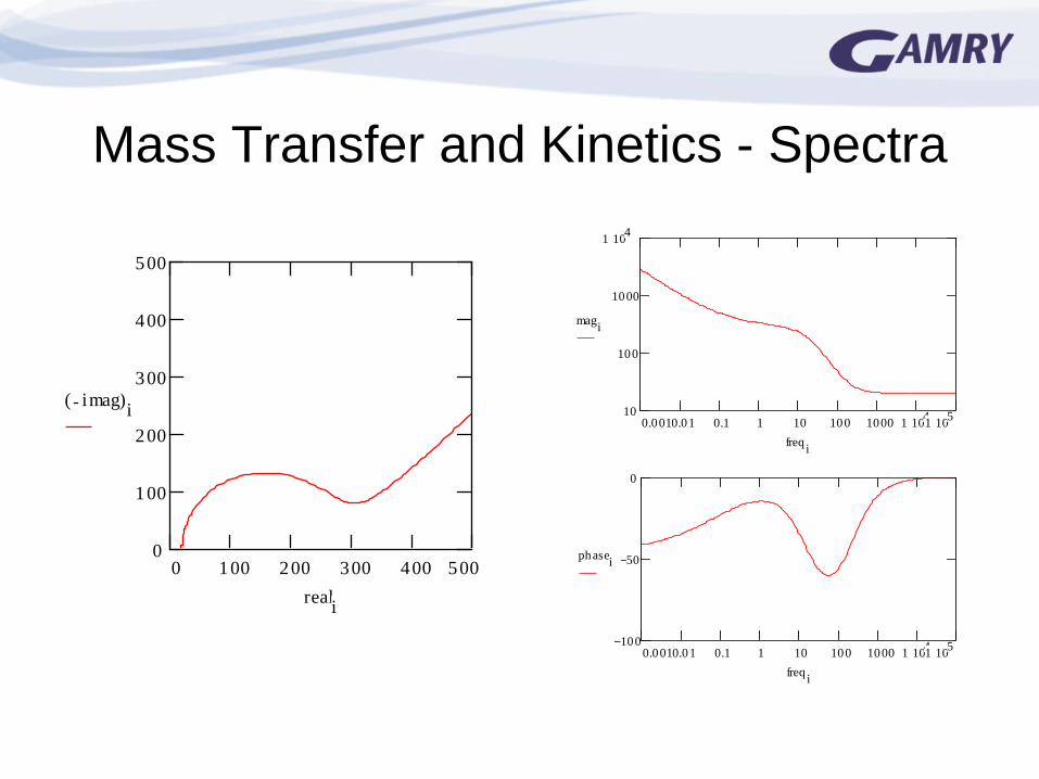
Mass Transfer and Kinetics - Spectra
0
100
200
300
400
500
0 100 200 300 400 500
( )imagi
reali
10
100
1000
1 104
0.0010.01 0.1 1 10 100 1000 1 1041 10
5
magi
freqi
100
50
0
0.0010.01 0.1 1 10 100 1000 1 1041 10
5
phasei
freqi
EIS Modeling
• Complex systems may require complex
models.
• Each element in the equivalent circuit should
correspond to some specific activity in the
electrochemical cell.
• It is not acceptable to simply add elements
until a good fit is obtained.
• Use the simplest model that fits the data.
Criteria For Valid EIS Linear – Stable - Causal
• Linear: The system obeys Ohm’s Law, E = iZ. The value of Z is independent of the magnitude of the perturbation. If linear, no harmonics are generated during the experiment.
• Stable: The system does not change with time and returns to its original state after the perturbation is removed.
• Causal: The response of the system is due only to the applied perturbation.
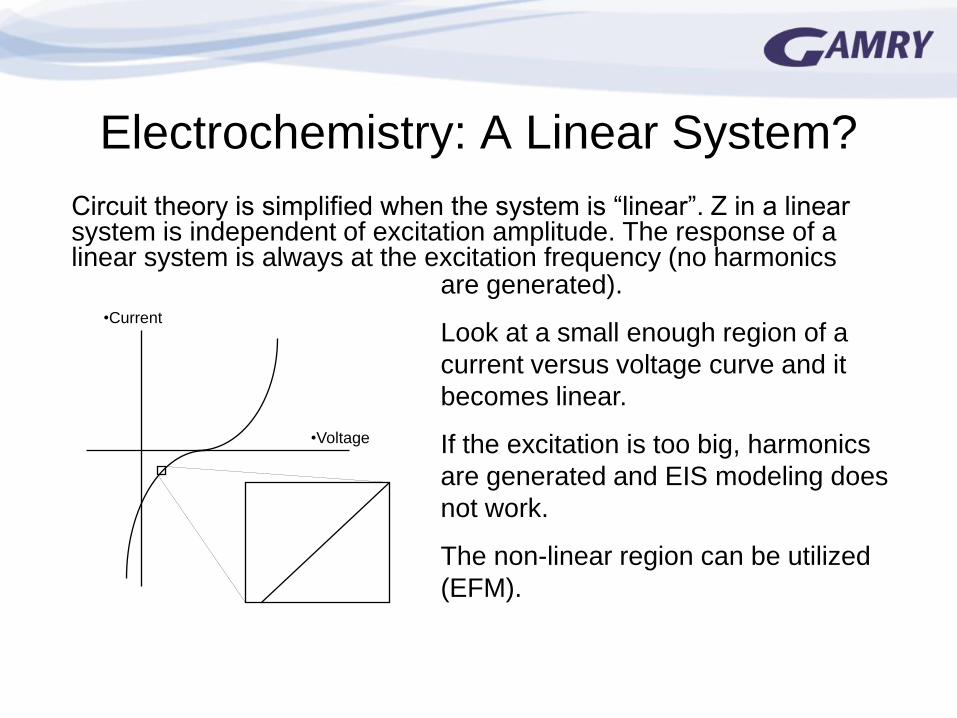
Electrochemistry: A Linear System?
Circuit theory is simplified when the system is “linear”. Z in a linear system is independent of excitation amplitude. The response of a linear system is always at the excitation frequency (no harmonics
are generated).
Look at a small enough region of a
current versus voltage curve and it
becomes linear.
If the excitation is too big, harmonics
are generated and EIS modeling does
not work.
The non-linear region can be utilized
(EFM).
•Current
•Voltage
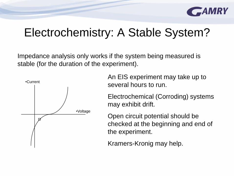
Electrochemistry: A Stable System?
Impedance analysis only works if the system being measured is
stable (for the duration of the experiment).
An EIS experiment may take up to
several hours to run.
Electrochemical (Corroding) systems
may exhibit drift.
Open circuit potential should be
checked at the beginning and end of
the experiment.
Kramers-Kronig may help.
•Current
•Voltage
Kramers-Kronig Transform
• The K-K Transform states that the phase and magnitude in a
real (linear, stable, and causal) system are related.
• Apply the Transform to the EIS data. Calculate the magnitude
from the experimental phase. If the calculated magnitudes
match the experimental magnitudes, then you can have some
confidence in the data. The converse is also true.
• If the values do not match, then the probability is high that your
system is not linear, not stable, or not causal.
• The K-K Transform as a validator of the data is not accepted by
all of the electrochemical community.
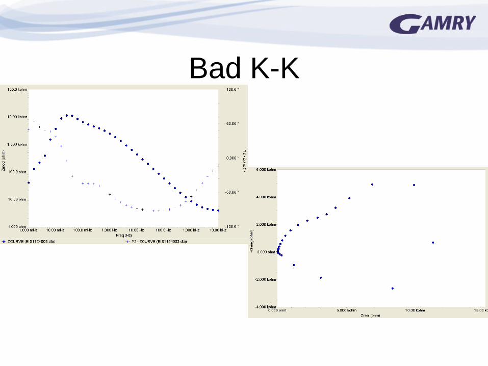
Bad K-K
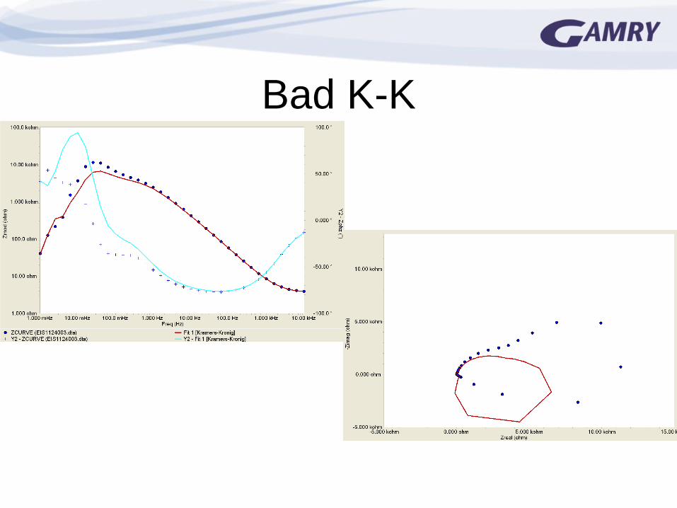
Bad K-K
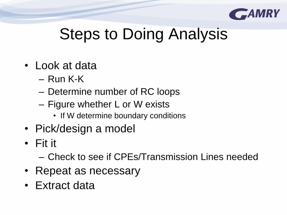
Steps to Doing Analysis
• Look at data – Run K-K
– Determine number of RC loops
– Figure whether L or W exists • If W determine boundary conditions
• Pick/design a model
• Fit it – Check to see if CPEs/Transmission Lines needed
• Repeat as necessary
• Extract data
EIS Instrumentation
• Potentiostat/Galvanostat
• Sine wave generator
• Time synchronization (phase locking)
• All-in-ones, Portable & Floating Systems
Things to be aware of…
• Software – Control & Analysis
• Accuracy
• Performance limitations
EIS Take Home
• EIS is a versatile technique
– Non-destructive
– High information content
• Running EIS is easy
• EIS modeling analysis is very powerful
– Simplest working model is best
– Complex system analysis is possible
– User expertise can be helpful

References for EIS
• Electrochemical Impedance and Noise, R. Cottis and S.
Turgoose, NACE International, 1999. ISBN 1-57590-093-9.
An excellent tutorial that is highly recommended.
• Electrochemical Techniques in Corrosion Engineering, 1986,
NACE International
Proceedings from a Symposium held in 1986. 36 papers.
Covers the basics of the various electrochemical techniques and
a wide variety of papers on the application of these techniques.
Includes impedance spectroscopy.
• Electrochemical Impedance: Analysis and Interpretation, STP
1188, Edited by Scully, Silverman, and Kendig, ASTM, ISBN 0-
8031-1861-9.
26 papers covering modeling, corrosion, inhibitors, soil,
concrete, and coatings.
• EIS Primer, Gamry Instruments website, www.gamry.com


