Research Journal of Finance and Accounting www.iiste.org
ISSN 2222-1697 (Paper) ISSN 2222-2847 (Online)
Vol.5, No.15, 2014
191
Effect of Oil Price Movement on Stock Prices in the Nigerian
Equity Market
Chukwunonso T. Okany*
International Training Institute, Central Bank of Nigeria.
Abstract
This paper studies the relationship between oil prices and stock prices in the Nigerian equity market using a
forecasting framework. The study was driven by the need to determine if the extreme volatility observed in oil
prices has any significant impact on the stock price movement of a major oil exporting economy like the Nigeria.
By establishing the presence of a significant relationship between these variables, investors and policymakers
alike could use oil prices as a leading indicator in producing more accurate projections of stock prices. While the
results of this study recorded no cointegration between stock prices and oil prices, the use of an ARIMA and a
structural-ARIMA model showed that oil price is a significant exogenous variable which could improve the
accuracy of stock price prediction in the Nigerian stock market by an extent.
Keywords: Oil prices, stock market predictability, Nigerian Stock Exchange.
1. Introduction
The documentation of the effects of oil prices on financial markets in developed economies like the United
States and a number of oil importing European markets has led to a relatively high interest in the study of
economic relationship between oil prices and the economic activities of these nations. One of such studies by
Jones and Kaul (1996) showed that oil price movement had a negative relationship with stock market prices. The
logic behind their conclusion could be explained by the fact that rising oil prices is associated with a rise in
energy costs which is central to the cost of production. With a rising cost of production, investors tend to devalue
firms due to lower expected returns in line with the concept of the weighted average cost of capital.
While there is a reasonably large and increasing literature on the impact of oil prices on stock prices for
developed markets, the same cannot be said for emerging oil exporting economies that profit from high oil prices.
This paper is aimed at deepening the study of the relationship between oil prices and movement of stock prices
in the emerging stock market of Nigeria. While a significant number of studies used the framework of employing
vector error correction models to model the impact of oil price shocks on stock market prices, this paper would
make use of a forecasting framework according to Ikoku and Okany (2010), using an ARIMA and a Structural-
ARIMA model to evaluate the impact of oil price movements on stock prices in Nigeria. My line of thought is
that if a combination of an ARMA terms and oil prices produces more accurate out of sample forecasts than an
ARIMA model, then it would be safe to conclude that oil price movements contains information which could
significantly reduce the forecast error of stock prices.
The second section of this paper reviews existing literature on studies bordering the relationship between oil
prices and stock market prices in both developed and emerging economies as well as oil importing and exporting
economies. Following the review of literature is a section dedicated to a number of statistics tests as well as the
modeling of stock prices followed by concluding sections detailing the findings and implications of the analysis.
*The views expressed in this paper are those of the author alone and do not necessarily represent those of the
Central Bank of Nigeria or CBN policy.
2. Literature Review
In one of the studies of oil price movement’s impact on stock prices and the economy, Barsky and Kilian (2002)
explained that one of the impacts of oil price shocks on stock prices was noted in the 70’s when a rise in oil
prices brought about by a severe decrease in the supply of oil resulted in a shortage of finished goods; this led to
a rise in the general price level of goods, and ultimately a global recession. While accepting the impact of oil
prices on the economy and financial markets however, Barsky and Kilian (2002) explained that the events of the
70’s which led to the various negative effects were more severe due to the economic climate of the period which
kept the demand for oil at a high, thereby amplifying the effect of the oil supply shock on the economy.

Research Journal of Finance and Accounting www.iiste.org
ISSN 2222-1697 (Paper) ISSN 2222-2847 (Online)
Vol.5, No.15, 2014
192
Although Barsky and Kilian blamed the recession on the oil price shock experienced during this period, there
have been other views which do not support the existence of a significant relationship between these two
variables. Chen et.al (1986) studied the impact of oil prices on what they would term, “the over-reaction of stock
market prices”. Establishing that stock market prices reacted to a number of economic events and the expectation
of such events, they point out that as a result of the portfolio diversification technique employed by financial
investors worldwide, the impact of oil price shocks on prices was not as significant as it was made to look. They
argued that factors more central to the determination of stock price movements were factors like discount rates,
monetary supply and other state factors which had a more significant impact on the financial markets.
Paying greater attention to the method used in determining the relationship between stock market prices and
certain macroeconomic variables including oil prices, Cheung and Lilian (1998) give less credit to conclusions
based on the short term relationship between oil prices and stock markets, arguing that a long term relationship
between these two variables provided more insight into stock price movement. Building the platform for their
study on the Engel Granger cointegration technique, they attempt to determine if indeed there was a long term
relationship and the dynamics of this relationship in five nations including Canada, Germany, Italy, Japan and the
United States. Having determined this relationship, they progressed by developing an error correction model to
improve their understanding of the impact of certain macroeconomic variables including oil prices on stock
market prices. The result of their tests gave more support to the existence of a long term relationship between the
two variables.
Adopting the same framework as Cheung and Lilian, Apergis and Miller (2008) employ the cointegration test
along with an error correction model in a wider selection of countries which included the United Kingdom and
France, they rejected the notion that there exists a very significant relationship between oil price shocks and
stock prices, arguing that while there was relationship, it was not a very significant relationship thereby
discrediting previous findings to the contrary.
So far, most of the reviewed studies on stock market returns and oil prices have been focused on developed
economies; one of the few studies that focused on emerging stock markets, including South Africa and
Venezuela, was by Basher and Sadorsky (2006) using data from a broad range of stock markets across emerging
markets. Their finding was that oil prices did have a strong impact on stock market returns in general. Their
method was based on the arbitrage pricing theory where oil price was used as a factor under investigation.
Another study by Faff and Brailsford (1999) on the Australian economy also suggested a significant relationship
between stock prices and oil prices while noting a negative relationship.
Also, Arouri and Rault (2010) studied the relationship oil price movements on stock prices of Gulf Corporation
Countries (GCC) to determine what causes what. They employed the granger causality test to determine the
causal effects between stock prices and oil prices. For the Saudi Arabian market, they found out that there was a
consistent bi-directional causality between the two variables, while for the other GCC countries there was a
unidirectional causality from oil prices to stock prices.
3. Data and Methodology
Data on the Nigerian stock market index (All-Share Index) was obtained from the Nigerian Stock Exchange
database. Taking end of month values of the index (ASI), which is value weighted and constitutes all traded
securities, the author used data from January 2004 to June 2014 making for 126 observations. I also obtained
monthly prices for Brent Crude from the Bloomberg database ranging from January 2004 to June 2014 making
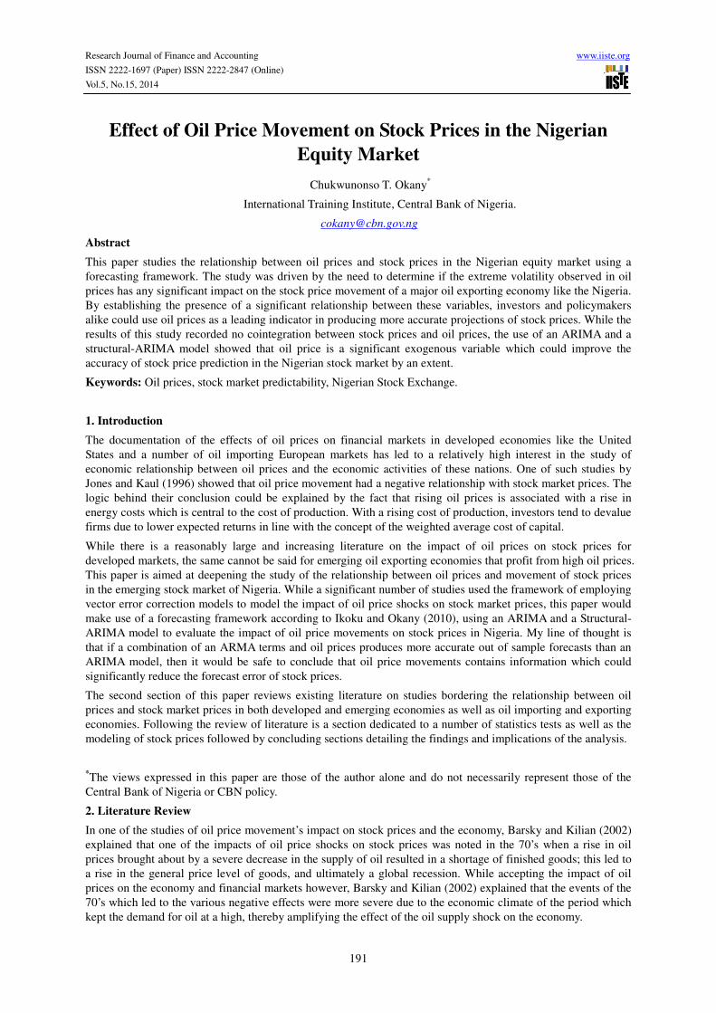
for an equal 126 observations. Please refer to figures 1, 2 and 3 for graphs of the data over this time period. Also,
Figures 5 and 6 shows the descriptive statics of the time series. A set of diagnostics is carried out on both
variables including tests for stationarity, causal effects and cointegration.

Research Journal of Finance and Accounting www.iiste.org
ISSN 2222-1697 (Paper) ISSN 2222-2847 (Online)
Vol.5, No.15, 2014
193
Figure 1. Historical movement of the Nigerian All-Share Index
Figure 2. Historical movement of Oil Prices
Research Journal of Finance and Accounting www.iiste.org
ISSN 2222-1697 (Paper) ISSN 2222-2847 (Online)
Vol.5, No.15, 2014
194
Figure 3. Historical movement of the Nigerian All-Share Index and Oil Prices
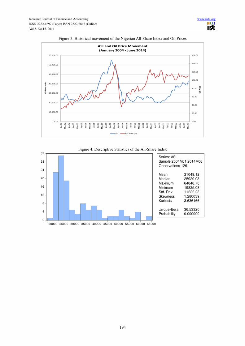
Figure 4. Descriptive Statistics of the All-Share Index
0.00
20.00
40.00
60.00
80.00
100.00
120.00
140.00
160.00
0.00
10,000.00
20,000.00
30,000.00
40,000.00
50,000.00
60,000.00
70,000.00
Jan-
04
May
-04
Sep-
04
Jan-
05
May
-05
Sep-
05
Jan-
06
May
-06
Sep-
06
Jan-
07
May
-07
Sep-
07
Jan-
08
May
-08
Sep-
08
Jan-
09
May
-09
Sep-
09
Jan-
10
May
-10
Sep-
10
Jan-
11
May
-11
Sep-
11
Jan-
12
May
-12
Sep-
12
Jan-
13
May
-13
Sep-
13
Jan-
14
May
-14
All-
Shar
e In
dex
ASI and Oil Price Movement
(January 2004 - June 2014)
ASI Oil Price ($)
Oil
Pric
e
0
4
8
12
16
20
24
28
32
20000 25000 30000 35000 40000 45000 50000 55000 60000 65000
Series: ASISample 2004M01 2014M06Observations 126
Mean 31049.12Median 25920.03Maximum 64848.70Minimum 19825.08Std. Dev. 11222.23Skewness 1.280039Kurtosis 3.636166
Jarque-Bera 36.53320Probability 0.000000
Research Journal of Finance and Accounting www.iiste.org
ISSN 2222-1697 (Paper) ISSN 2222-2847 (Online)
Vol.5, No.15, 2014
195
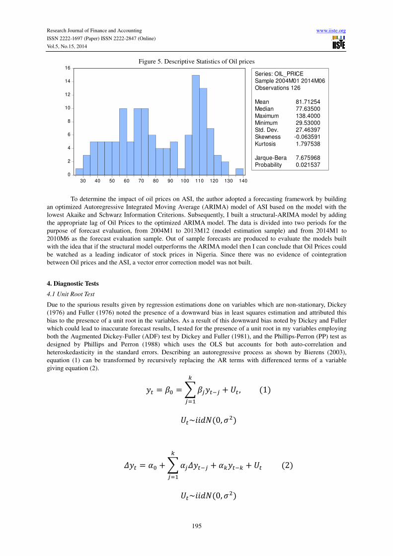
Figure 5. Descriptive Statistics of Oil prices
To determine the impact of oil prices on ASI, the author adopted a forecasting framework by building
an optimized Autoregressive Integrated Moving Average (ARIMA) model of ASI based on the model with the
lowest Akaike and Schwarz Information Criterions. Subsequently, I built a structural-ARIMA model by adding
the appropriate lag of Oil Prices to the optimized ARIMA model. The data is divided into two periods for the
purpose of forecast evaluation, from 2004M1 to 2013M12 (model estimation sample) and from 2014M1 to
2010M6 as the forecast evaluation sample. Out of sample forecasts are produced to evaluate the models built
with the idea that if the structural model outperforms the ARIMA model then I can conclude that Oil Prices could
be watched as a leading indicator of stock prices in Nigeria. Since there was no evidence of cointegration
between Oil prices and the ASI, a vector error correction model was not built.
4. Diagnostic Tests
4.1 Unit Root Test
Due to the spurious results given by regression estimations done on variables which are non-stationary, Dickey
(1976) and Fuller (1976) noted the presence of a downward bias in least squares estimation and attributed this
bias to the presence of a unit root in the variables. As a result of this downward bias noted by Dickey and Fuller
which could lead to inaccurate forecast results, I tested for the presence of a unit root in my variables employing
both the Augmented Dickey-Fuller (ADF) test by Dickey and Fuller (1981), and the Phillips-Perron (PP) test as
designed by Phillips and Perron (1988) which uses the OLS but accounts for both auto-correlation and
heteroskedasticity in the standard errors. Describing an autoregressive process as shown by Bierens (2003),
equation (1) can be transformed by recursively replacing the AR terms with differenced terms of a variable
giving equation (2).
�� = �� =������� + � ,�
� �(1)
�~����(0, ��)
��� = �� +�������� + ������ + �(2)�
� �
�~����(0, ��)
0
2
4
6
8
10
12
14
16
30 40 50 60 70 80 90 100 110 120 130 140
Series: OIL_PRICESample 2004M01 2014M06Observations 126
Mean 81.71254Median 77.63500Maximum 138.4000Minimum 29.53000Std. Dev. 27.46397Skewness -0.063591Kurtosis 1.797538
Jarque-Bera 7.675968Probability 0.021537

Research Journal of Finance and Accounting www.iiste.org
ISSN 2222-1697 (Paper) ISSN 2222-2847 (Online)
Vol.5, No.15, 2014
196
where �� = ��, �� = ∑ �� � 1, � = 1,… , !.�� �
I apply the ADF and PP test to the ASI and Oil Prices where the presence of a unit root is indicated when �� = 0
as the null hypothesis (#�), against an alternative hypothesis (#�) when �� $ 0, which indicates the absence
of a unit root.
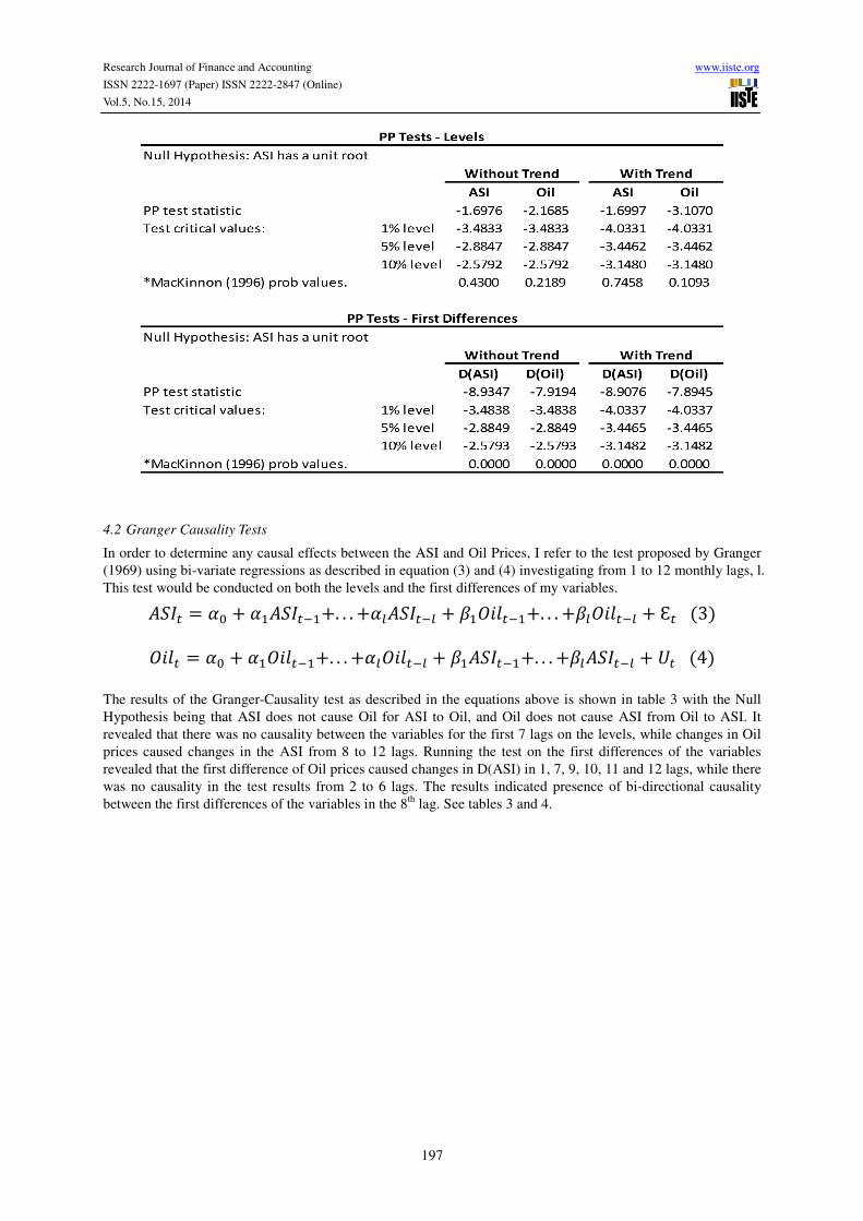
In general, the results of the unit root tests on the two times series, ASI and Oil prices, indicated the presence of a
unit root in the two financial time series. I conducted the tests with and without assumptions of a linear trend in
the series since I could not determine visually whether the series had a linear trend. The ADF test revealed that
ASI and Oil prices had a unit root on the levels without trend, while testing with assumptions of a linear trend
showed that there was a unit root in the ASI and none in the Oil Prices, with a prob. value of 0.0379 rejecting the
presence of a unit root in the Oil prices assuming a linear trend. However, the results differed with the PP test
which showed the presence of a unit root in the two variables both with and without a trend for both the ASI and
Oil prices on the levels.
In order to clean up the unit roots noted in the variables on the levels, I ran the tests on the first differences of the
series; the results from both the ADF and PP tests strongly rejected the presence of unit roots in the first
differences with and without trend as depicted in table 1 and 2 respectively.
Table 1. Unit Root Tests (Augmented Dickey-Fuller)
Table 2. Unit Root Tests (Phillips-Perron)
Research Journal of Finance and Accounting www.iiste.org
ISSN 2222-1697 (Paper) ISSN 2222-2847 (Online)
Vol.5, No.15, 2014
197
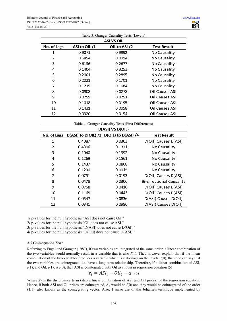
4.2 Granger Causality Tests
In order to determine any causal effects between the ASI and Oil Prices, I refer to the test proposed by Granger
(1969) using bi-variate regressions as described in equation (3) and (4) investigating from 1 to 12 monthly lags, l.
This test would be conducted on both the levels and the first differences of my variables.
%&'� = �� + ��%&'���+. . . +�(%&'��( + ��)�*���+. . . +�()�*��( + Ԑ�(3) )�*� = �� + ��)�*���+. . . +�()�*��( + ��%&'���+. . . +�(%&'��( + � (4)
The results of the Granger-Causality test as described in the equations above is shown in table 3 with the Null
Hypothesis being that ASI does not cause Oil for ASI to Oil, and Oil does not cause ASI from Oil to ASI. It
revealed that there was no causality between the variables for the first 7 lags on the levels, while changes in Oil
prices caused changes in the ASI from 8 to 12 lags. Running the test on the first differences of the variables
revealed that the first difference of Oil prices caused changes in D(ASI) in 1, 7, 9, 10, 11 and 12 lags, while there
was no causality in the test results from 2 to 6 lags. The results indicated presence of bi-directional causality
between the first differences of the variables in the 8th
lag. See tables 3 and 4.
Research Journal of Finance and Accounting www.iiste.org
ISSN 2222-1697 (Paper) ISSN 2222-2847 (Online)
Vol.5, No.15, 2014
198
Table 3. Granger Causality Tests (Levels)
Table 4. Granger Causality Tests (First Differences)
1/ p-values for the null hypothesis "ASI does not cause Oil."
2/ p-values for the null hypothesis "Oil does not cause ASI."
3/ p-values for the null hypothesis "D(ASI) does not cause D(Oil)."
4/ p-values for the null hypothesis "D(Oil) does not cause D(ASI)."
4.3 Cointegration Tests
Referring to Engel and Granger (1987), if two variables are integrated of the same order, a linear combination of
the two variables would normally result in a variable that is also I(1). They however explain that if the linear
combination of the two variables produces a variable which is stationary on the levels, I(0), then one can say that
the two variables are cointegrated, i.e. have a long term relationship. Therefore, if a linear combination of ASI,
I(1), and Oil, I(1), is I(0), then ASI is cointegrated with Oil as shown in regression equation (5) .� = %&'� � )�*� � � (5)
Where .� is the disturbance term (also a linear combination of ASI and Oil prices) of the regression equation.
Hence, if both ASI and Oil prices are cointegrated, .� would be I(0) and they would be cointegrated of the order
(1,1), also known as the cointegrating vector. Also, I make use of the Johansen technique implemented by

Research Journal of Finance and Accounting www.iiste.org
ISSN 2222-1697 (Paper) ISSN 2222-2847 (Online)
Vol.5, No.15, 2014
199
Johansen (1991) using VAR systems which requires the two variables in the linear combination to be integrated
of the same order. For fairness in testing for cointegration between ASI and oil prices, I tested the two variables
for a cointegration relationship using the Phillips-Ouliaris cointegration test as applied by Bernard and Durlauf
(1995).
Table 5 shows the results of my test using the Johansen technique which revealed that there was no long run
relationship between ASI and Oil prices. The test was conducted with no restrictions on the cointegrating
equation, assuming an intercept and no linear trend in the CE. The trace test failed to reject the null hypothesis of
no cointegration equation at the 5 percent level with a prob value of 0.4899. The maximum-Eigenvalue also
failed to reject the absence of a long run relationship between the two variables in the long run with a prob. value
of 0.6492. Also, in table 6, the two step Engel-Granger test revealed that there was no cointegration between ASI
and Oil prices with a prob. value of 0.8778 on the tau-statistics, and 0.8935 on the z-statistic accepting the null
hypothesis of no cointegration between the two. The Phillips-Ouliaris test also shown in table 7 goes on to
confirm that there was no long run relationship between ASI and Oil prices.
Table 5. Johansen Cointegration Test
Table 6. Engle-Granger Cointegration Test
Table 7. Phillip-Ouliaris Cointegration

Research Journal of Finance and Accounting www.iiste.org
ISSN 2222-1697 (Paper) ISSN 2222-2847 (Online)
Vol.5, No.15, 2014
200
5.0 Forecast Models and Performance
Maintaining the choice of a forecasting framework, the author built an ARIMA model as proposed by Box and
Jenkins (1976) by selecting the model with the lowest AIC from a total of 64 models of D(ASI), using AR and
MA terms as shown in table 8. The best ARIMA model obtained was an ARIMA (2, 1, 2) with an SIC of 18.4087
and Adjusted R-Square of 17.68 percent. Using this as my bench mark model, I developed a structural ARIMA,
using the first difference of Oil prices as an explanatory variable of the All-Share index. The structural model
which recorded an Adjusted R-Square of 24.91 percent showed that D(Oil(-1)) was significant in the model with
a coefficient of 64.5228 and a t-statistic of 2.5893. The correlogram of residuals for ARIMA and the structural
model (SARIMA) are shown in tables 10 and 11 respectively. Due to the lack of cointegration between the two
variables, the use of an Error Correction Model to capture any long run dynamics between the variables is ruled
out. Both models are presented in table 9.
With these two models, I produce an out of sample forecast with different time horizons, 2 months, 4 months and
6 months. The results of the two models were evaluated using the mean absolute percent error (MAPE) as shown
in equation 6
/%01 = 100 � 2%&'�3�%&'�%&'� 2(6)567
� 56�
where %&'�-hat at time-t is the forecast and %&'� is the actual.
The results of the forecast shown in table 12 showed that the structural model with Oil prices as an additional
exogenous variable outperformed the ARIMA model in the 2 and 4 months forecast horizon. In the 2 months
forecast, the structural model with Oil prices had an MAPE of 6.687 percent against the ARIMA’s 7.036 percent,
while in the 4 month forecasts, the structural model had 11.3902 percent against the ARIMA’s 11.6369 percent.
In the longest forecast horizon adopted (6 months), the structural model recorded an MAPE of 10.0698 percent
against the ARIMA’s 9.8442 percent. Noticeable is that as the horizon becomes longer, the forecast accuracy
reduced which could be attributed to the lack of cointegration between the two from the tests conducted.
Table 8. ARIMA Selection by SIC
AR / MA 0 1 2 3 4 5 6 7
0 18.4694 18.4684 18.4335 18.4356 18.4457 18.4551 18.4893 18.5142
1 18.4541 18.4399 18.4571 18.4269 18.4631 18.4994 18.4631 18.5000
2 18.4351 18.4678 18.4087 18.4574 18.4488 18.4465 18.5477 18.5862
3 18.4443 18.4358 18.4670 18.4737 18.5354 18.4676 18.4992 18.5401
4 18.4510 18.4720 18.4507 18.4903 18.5511 18.5110 18.5517 18.5361
5 18.4786 18.5142 18.5358 18.5594 18.5565 18.5620 18.5362 18.5775
6 18.5041 18.5372 18.5255 18.5595 18.5744 18.6047 18.5798 18.6148
7 18.5444 18.5865 18.5609 18.6005 18.5890 18.6258 18.6634 18.6623
ARIMA MODEL SELECTION BY SIC

Research Journal of Finance and Accounting www.iiste.org
ISSN 2222-1697 (Paper) ISSN 2222-2847 (Online)
Vol.5, No.15, 2014
201
Table 9. Forecast Model and Performance

Research Journal of Finance and Accounting www.iiste.org
ISSN 2222-1697 (Paper) ISSN 2222-2847 (Online)
Vol.5, No.15, 2014
202
Table 10. Correlogram (ARIMA)

Research Journal of Finance and Accounting www.iiste.org
ISSN 2222-1697 (Paper) ISSN 2222-2847 (Online)
Vol.5, No.15, 2014
203
Table 11. Correlogram (Structural-ARIMA)

Research Journal of Finance and Accounting www.iiste.org
ISSN 2222-1697 (Paper) ISSN 2222-2847 (Online)
Vol.5, No.15, 2014
204
Table 12. Forecast Performance
6.0 Conclusion
The results from my analysis shows that while there was no long run relationship between the ASI and Oil prices,
there appeared to be a short run relationship between the two variables. Going by the forecasting framework
adopted, the results show that Oil prices when used to model stock prices in the Nigerian stock market, did
marginally reduce forecast errors in two of the three adopted forecast horizons, and could be said to have some
predictive ability as a result. This might not be unconnected with the fact that Oil is the main source of revenue
for the Nigerian economy; hence changes in oil prices could have an effect on stock prices. The findings in this
study have significant implications in that it gives investors and policymakers alike, an important perspective on
the oil price risk inherent in the Nigerian stock market. However, upon the conclusion of this study, I believe that
a better predictor of stock prices in the Nigerian stock market might be revenue from oil sales. Because this is the
main source of revenue for the economy, it might have a more significant relationship with stock market prices
as a result. More research could be carried on this area to enrich existing literature on the subject.
Research Journal of Finance and Accounting www.iiste.org
ISSN 2222-1697 (Paper) ISSN 2222-2847 (Online)
Vol.5, No.15, 2014
205
References
Apergis, N. and S.M. Miller, 2008, “Do Structural Oil-Market Shocks Affect Stock Prices?” University of
Connecticut, Economics Department working paper.
Arouri, M.E.H., and C. Rault., 2010, “Oil Prices and Stock Markets: What Drives what in the Gulf Corporation
Council Countries?” CESifo working paper series, No. 2934.
Barsky, R.B., and L. Kilian, 2001, “Do We Really Know that Oil Caused The Great Stagflation? A Monetary
Alternative,” NBER Macroeconomics Annual 2001, MIT Press, Vol. 16.
Basher, S.A., and P. Sardosky, 2006, “Oil Price Risk and Emerging Stock Markets,” Global Finance Journal, Vol.
17, pp. 224 – 251.
Bernard, A.B., and S.N. Durlauf, 1995, “Convergence in international Output”, Journal of Applied Econometrics,
Vol. 10, pp. 97 – 108.
Bierens, H., 2003, Unit Roots, in Baltagi, B., (editor), A Companion to Theoretical Econometrics, Blackwell
Publishing, 2003.
Box, George E.P. and Gwilyn M. Jenkins, 1976, Time Series Analysis: Forecasting and Control, Revised Edition,
Oakland, CA: Holden-Day
Chen, N., R. Roll., and S.A. Ross, 1986, “Economic Forces and the Stock Market”, The Journal of Business, Vol.
59, No. 3, Pp. 383 – 403.
Cheung, Y., and K.N. Lilian, 1998, “International Evidence on the Stock Market and Aggregate Economic
Activity,” Journal of Empirical Finance, Vol. 5, pp. 281 – 296.
Dickey, D.A., 1976, Estimation and Hypothesis Testing in Nonstationary Time Series, Ph.D. dissertation, Iowa
State University.
Dickey, D.A. and W.A. Fuller, 1981, “Likelihood Ratio Statistics for Autoregressive Time Series with a Unit
Root,” Econometrica, Vol. 49, pp. 1057-1072.
Engle, R. F. and C.W. Granger, 1987, “Cointegration and Error Correction: Representation, Estimation and
Testing,” Econometrica, Vol. 55, pp. 251-276.
Faff, R.W., and T.J. Brailsford, 1999, “Oil Price Risk and the Australian Stock Market,” Journal of Energy
Finance and Development, Vol. 4, pp. 69 – 87.
Fama, E.F., 1970, “Efficient Capital Markets: A review of theory and empirical work,” Journal of Finance, pp.
383 – 417.
Fuller, W.A., 1976, Introduction to Statistical Time Series. New York: Wiley.
Granger, C. J., 1969, "Investigating Causal Relationships by Econometrics Models and Cross Spectral Methods,"
Econometrica, Vol. 37, pp. 425-435.
Ikoku, A.E. and C.T Okany, 2010, “Can Price Earning rations predict stock prices?”, International Journal of
Finance, Vol. 22, pp. 6581.
Jones, C.M. and G. Kaul, 1996, “Oil and the Stock Markets,” Journal of Finance, Vol. 51, pp 463 – 491.
Johansen, S., 1991, "Estimation and Hypothesis Testing of Cointegration Vectors in Gaussian Vector
Autoregressive Models," Econometrica, Vol. 59, pp. 1551-1580.
Phillips, P.C. and P. Perron, 1988, “Testing for a Unit Root in Times Series Regression”, Biometrika, Vol. 75, pp.
335-346.
Phillips, P.C. and S. Ouliaris, 1990, “Asymptotic Properties of Residual Based Tests for Cointegration”,
Econometrica, Vol. 58, No. 1, pp.165–193.

The IISTE is a pioneer in the Open-Access hosting service and academic event
management. The aim of the firm is Accelerating Global Knowledge Sharing.
More information about the firm can be found on the homepage:
http://www.iiste.org
CALL FOR JOURNAL PAPERS
There are more than 30 peer-reviewed academic journals hosted under the hosting
platform.
Prospective authors of journals can find the submission instruction on the
following page: http://www.iiste.org/journals/ All the journals articles are available
online to the readers all over the world without financial, legal, or technical barriers
other than those inseparable from gaining access to the internet itself. Paper version
of the journals is also available upon request of readers and authors.
MORE RESOURCES
Book publication information: http://www.iiste.org/book/
IISTE Knowledge Sharing Partners
EBSCO, Index Copernicus, Ulrich's Periodicals Directory, JournalTOCS, PKP Open
Archives Harvester, Bielefeld Academic Search Engine, Elektronische
Zeitschriftenbibliothek EZB, Open J-Gate, OCLC WorldCat, Universe Digtial
Library , NewJour, Google Scholar


