
11 HOLMAN WAY, ORANGE, NSW, AUSTRALIA T [email protected] U WWW.ECHIDNAMMS.ORG
Cargo Vale
Echidna Mixed Model Software For use in biological science 16 February 2019

Cargo Vale | Echidna Mixed Model Software
2
Preface This document describes software written to facilitate the statistical analysis of
biological data using linear mixed models. It builds on over 40 years of experience of
the lead developers in applied biometry in agriculture.
The Echidna project aims to provide software similar to ASReml (copyright VSN
International, www.vsni.co.uk). We expect it will provide most of the facilities in
ASReml, and more with similar or better performance. By arrangement with VSN,
Echidna may be used by ASReml licensees and for non-commercial purposes (academic,
research). It is expected improved functionality in Echidna will be implemented in
ASReml in due course.
We live in a world that seems so simple, yet is incredibly complex when you lift the
bonnet. Solomon said “It is the glory of God to conceal a matter, But the glory of kings
is to search out a matter.” (Proverbs 25:2). Linear models have proven very effective at
analyzing data and gaining an understanding of how things work, with a view to
overcoming production issues for food and fibre.
The echidna is an Australian form of spiny ant-eater. It is an egg laying mammal, a
monotreme, and remarkably efficient at digging for ants. We hope Echidna, a name
given to this software, will prove an efficient tool for investigators digging for
knowledge.
We could wait until the product is well developed and tested before releasing it, but
time is short and tomorrow never comes. So we leave it to you to decide if this product
is useful to you in its current state.
This product is dedicated to the glory of the God and Father of our Lord and Saviour,
Jesus Christ who seeks to bring many sons into His kingdom.
Arthur Gilmour

Cargo Vale | Echidna Mixed Model Software
3
22 Then Paul stood in the midst of the Areopagus and said, “Men of Athens, I perceive
that in all things you are very religious; 23 for as I was passing through and considering
the objects of your worship, I even found an altar with this inscription:
TO THE UNKNOWN GOD.
Therefore, the One whom you worship without knowing, Him I proclaim to you: 24
“God, who made the world and everything in it, since He is Lord of heaven and earth,
does not dwell in temples made with hands. 25 Nor is He worshiped with men’s hands,
as though He needed anything, since He gives to all life, breath, and all things. 26 And
He has made from one blood[c] every nation of men to dwell on all the face of the
earth, and has determined their pre-appointed times and the boundaries of their
dwellings, 27 so that they should seek the Lord, in the hope that they might grope for
Him and find Him, though He is not far from each one of us; 28 for in Him we live and
move and have our being, as also some of your own poets have said, ‘For we are also
His offspring.’ 29 Therefore, since we are the offspring of God, we ought not to think
that the Divine Nature is like gold or silver or stone, something shaped by art and man’s
devising. 30 Truly, these times of ignorance God overlooked, but now commands all
men everywhere to repent, 31 because He has appointed a day on which He will judge
the world in righteousness by the Man whom He has ordained. He has given assurance
of this to all by raising Him from the dead.” Acts 17: 22-31
Cargo Vale | Echidna Mixed Model Software
4
Introduction This software currently comes only as a standalone program called Echidna. (An R
package based on the core has not yet been developed). The latest build of Echidna
can be downloaded from https://www.EchidnaMMS.org. Do not hesitate to report
issues to [email protected] as the developers would like to make this software
as robust and as useful as they can.
Echidna is used in a wide range of settings and therefore has many options (qualifiers)
which cater for the specific characteristics of some of those applications. This
necessarily makes documentation difficult because most qualifiers will not be relevant.
We therefore recommend you identify examples which are similar to your application
to see the things that may be relevant. Further detail on qualifiers may be obtained
from the ASReml User Guide – Functional syntax. Many of the applications are
explained in the new book Genetic Data Analysis for Plant and Animal Breeding by
Fikret Isik · James Holland Christian Maltecca, published by Springer.
Installation Installation is not automated. You will need to download the appropriate files for your
system and the system specific installation instructions.
The Windows implementation of Echidna comes as an archive (.zip file) with 3 folders.
The program Echidna.exe is in the bin folder, this User Guide is in the doc folder and the
examples discussed here are in the examples folder. Check the website for further
installation instructions.
Separate instructions and files are provided for Linux and Mac installations.
Support Echidna is not formally supported and comes with no warranty. No charge is made by
the developer for access to or use of Echidna. However, he will attempt to fix any bugs
that are reported and consider extending the functionality to meet the needs of users.
If you require statistical advice or training to use this software, you may be charged up
to AUD 285 per hour, according to your ability to pay. If you use this software for
commercial purposes, you must obtain an ASReml license from VSN

Cargo Vale | Echidna Mixed Model Software
5
Echidna End User Agreement I understand that 1. The Echidna program was developed by Arthur Gilmour who also did the bulk of the software development of ASReml while employed by NSW DPI 2. NSW DPI sold its interests in ASReml to VSN International who now own all its intellectual property rights 3. VSN consequently own all intellectual property rights associated with ASReml authorize ASReml licencees to use Echidna. They further authorize non-commercial use of Echidna. 4. Echidna is not intended as a replacement for ASReml but as a platform for testing developments that could be implemented in ASReml if VSN choose. 5. There is absolutely no warranty on this product. You use it at your own risk and are encouraged to test results with those from ASReml. I agree not to use Echidna for commercial purposes unless I have a current license to use ASReml. Commercial purposes include genetic evaluation to develop a product or to provide services for which you are paid. I acknowledge that my contact details will be given to VSN upon request.

Cargo Vale | Echidna Mixed Model Software
6
Echidna Source Code License
Agreement Requests for access to the Echidna Source code should be submitted via the website with a statement of intent. You will need to complete a collaborators agreement with VSN. In addition to the terms of the End User Agreement, you will agree not to distribute the source code to another person, and not to use the source code to create a product to be used contrary to the End User Agreement. Further, you will agree to submit any enhancements to the developers for potential inclusion in the main
product.

Cargo Vale | Echidna Mixed Model Software
7
JobFlow This section gives a description of the process of analyzing data with Echidna. The
detail is given in preceding sections.
A hypothesis. One must begin with a question, and collect data to explore the answer to
the question. This is normally expressed as a series of hypotheses which can be tested
in the data. Alternatively, one may wish to estimate an effect in which case you need to
collect enough data to provide sufficient accuracy to your estimate.
Some data. The data is then organized into a table where columns (fields) are variables
and rows are subjects/units/plots. Variables include response variables (measured on
the subjects), covariates (also measured) and descriptive information, factors or class
variables which characterize the subjects. One should include all such variables that
may influence the response. Some will be treatments which relate to your hypotheses
and others will be factors which contribute variation and need to be adjusted for. As
noted above, the data file typically has a header line containing simple column labels
which will be used to name the variables in the analysis, and is often prepared in Excel.
A command file. Now we prepare the basic command file by running Echidna on the
data file (assuming it has headings and has file extension .txt or .csv). This creates a
basic command file but it probably has not correctly classified the variables into variates
(always numeric) and factors (sometimes numeric, sometimes alphanumeric). So,
review the command file, run it and review the data summary reported in the .esr file.
You can further validate the data with PLOT and TABULATE statements.
Output files. Echidna puts its output into several files. You need to know what is in each
file. You will always view the .esr file. You should view the graphics file for the initial
analyses of every trait to check the residuals are plausible (in large datasets, you need
to specify !YHT to get the residuals (.esy) and plot of residuals). All these files are ASCII
files except for the graphics files.
Model Fitting. Typically, you will run a series of models, changing the command file
between runs, in the light of the preceding runs. Start with simple models to check the
data is properly interpreted, the degrees of freedom, numbers of effects, variances and
distribution of residuals are all plausible. Use the !PART/!DOPART mechanism to
maintain a record of the sequence of jobs. Use the command line qualifiers !RENAME,
!ARG and !OUTFILE to put the output files in separate folders.

Cargo Vale | Echidna Mixed Model Software
8
Reporting. VPREDICT and PREDICT are used to report functions of the variance
components (VPREDICT) or model summaries showing fitted means (PREDICT).
Extension Content
.es The command file
.esr Data summary, Analysis summary, Important messages
.esw Secondary information relating to the fitting process
.esl Diagnostic debugging information if requested !LOG !DEBUG
.ess Fitted effects from the model
.esy Residuals and fitted values from the fitted model
.esv Holds latest values of variance parameters
.esk Keeps track of details from the last run
.epv PREDICT output
.etb TABULATE output
.emf/.eps PLOT output (needs graphics viewer to view)
.evp VPREDICT output
Running Echidna You will need to use an ASCII text editor to create the command file and maybe a
spreadsheet program to save the data typically as a .csv (Comma Separated Values) file.
Then, from a command window, you can type
<Echidna Program Path> <Command File Name>
Windows
Some ASCII text editors enable you to run Echidna directly from the editor.
ConText
download from www.contexteditor.org and install
<Options> <Environment Variables> <Execute Keys>
<User exec keys|Add> enter [as,es,csv] and select F9 (say)
Cargo Vale | Echidna Mixed Model Software
9
<Execute> [<Echidna Program Path> ]
<Start in> enter [%p]
<Parameters> enter [%f]
<Hint> enter [Echidna]
<OK>
Then, if you have a .as or .es file open in the editor and press F9, Context will run
Echidna on the file.
Notepad++ (NPP)
download notepad++ (https://notepad-plus-plus.org/download/) and install it
The easiest way to get similar functionality to Context is to install the plugin NppExec.
First install (from https://github.com/bruderstein/nppPluginManager/releases) plugin
manager (will appear in the NPP Plugins menu) and use it to install NppExec (also into
the plugins menu). Use that to create a plugin script
cd $(FULL_CURRENT_PATH)
<Echidna Program Path> -o $(NAME_PART)
npp_open $(CURRENT_DIRECTORY)\$(NAME_PART).esr
and save it (say as Echidna). <F6> will call up the script and <OK> will run it.
Data Any analysis requires data. This might be obtained by conducting an experiment
following protocols to avoid bias and excessive noise in the observations, or by
observing and recording some aspect of creation.
Such data needs to be organized as variables and samples. These will typically be
recorded in a spread-sheet, or maybe a data base, with samples being rows and
variables being columns. Such a table may have millions of rows and thousands of
columns but we will begin with smaller data sets.
Variables are typically identifiers (names), class variables (categories) or measurements
(variates). The values of some variables may be missing for some samples.
The rows of data typically relate to individuals, plants, animals, plots and are often
called subjects/experimental units.

Cargo Vale | Echidna Mixed Model Software
10
Echidna typically reads the data from ASCII text files, often exported from Excel as a
COMMA separated (.csv) or TAB separated values.
It is usual to prepare the data file with a simple name/label for each variable (one
alphanumeric word beginning with a letter) on the first line. Use the !SKIP 1 qualifier to
skip over the line when reading the data. The line is there though to facilitate creating
the initial command file which needs names for the variables in order.
Missing values should be represented by NA, *(asterisk) or .(fullstop). In a .csv file or if
the !CSV qualifier is set, consecutive COMMAs or TABs also imply a missing value.
Command File The user must prepare a command file to run Echidna. This command file has 4 major
sections:
1. Top Control line: Instructions relating to running the job
2. Data description lines: define the input for the analysis
3. Model specification: defines the statistical model to be fitted
4. Output options:
The following sections provide basic and extended information on each phase of the
job.
The typical process is:
1. Run Echidna on the data file to produce a command file template
2. Adapt the file to properly reflect your intentions with respect to the use of each
variable (since the template may not correctly distinguish between variates and
class variables coded as integers)
3. Add the appropriate model line. (Start with a simple model, just to check the
data is being correctly interpreted by Echidna).
4. Run the model and review the output. The output consists of three or more
ASCII files, depending on output options selected and usually includes a plot of
residuals.
5. Modify the model, or add new models and run them, until your analysis is
complete.

Cargo Vale | Echidna Mixed Model Software
11
This guide is only an introduction to coding Echidna, with some basic reference
summaries. If you run the examples and understand the coding, you will be well on the
way to creating your own job. Hopefully, a Resources section of the web-site will present
more detailed explanations of particular cases.

Cargo Vale | Echidna Mixed Model Software
12
Top Command Line Please note the distinction between the command line and the top command line. The
former is the system command to invoke Echidna and under Windows might look like:
“C:\Program Files\ Echidna\bin\Echidna.exe” -w2ro oats 1
while the top command line is the first line of the Echidna command file (say oats.es)
and might look like:
!WORK 2 !RENAME !ARGS 1 !OUTFOLDER
In this case, both supply the same information to the job but the latter is often more
convenient. The latter may be omitted but if both are specified, both are honoured if
there is no conflict and otherwise the former takes precedence.
By the command line we mean the system command used to run Echidna. The
command line has 4 components.
1. The program pathname (under Windows, this might be
“C:\Program Files\Echidna\bin\Echidna.exe”, but it depends where you install
the program)
2. Run option string: This is a sequence of letters and numbers following a MINUS
character. This string is typically omitted as it is often easier to specify the
options on the top control line specified in the command file. Options specified
on the command line take precedence over the alternative specification on the
top control line. The options are described below. For example -w2
3. Command file name. If the command file name is not specified, Echidna will
prompt for the name of the working folder, and the name of the command file.
The command file name is typically a file with filename extension .es but to
create a template .es file, will be the name of the data file. For example oats
4. Arguments. Arguments are strings inserted into the command file at run time.
Options – top line qualifiers Qualifiers are the main way run time alternatives are controlled. Qualifiers begin with
the ! character followed by a name. While the name is usually more than 3 letters long,
it is sufficient to specify just the first three letters. Some qualifiers have arguments. An
argument of 0 is equivalent to not specifying the qualifier. When setting these
qualifiers via the command line options string, just use the first letter.
The top line qualifiers are defined in a typical order of specification:
Cargo Vale | Echidna Mixed Model Software
13
!WORKSPACE n
where n is an integer between 1 and 32 indicating gigabytes of workspace (1 is the
default)
!CONTINUE [f] or !FINAL [f]
instructs Echidna to retrieve variance parameters from an .esv file (f), if available and
continue iterating, or do just 1 more final iteration. If no .esv file is specified, Echidna
looks for one with the same name as the .esr file being produced. If there is none
present, it looks for a filename in the .esk file; when an .esv file is produced, its name is
saved in the .esk file.
!RENAME r
instructs Echidna to modify the output filename using the argument strings. If r is
specified (default 1), then r arguments are built into the output file name. If there are
more than r arguments, the job is run repeatedly for each argument in turn, with the
argument names built into the output file names.
!ARGS a1 [a2 …]
sets the argument strings. As well as the arguments being built into the output
filename, (see !RENAME), they are also substituted into the command file wherever $1
[$2 …] appear in the job. A common use is to specify which !PART of the command file
to process through the !DOPART process described below.
!OUTFOLDER [f]
used with !RENAME and ARGS causes the argument string to be built into the folder
name rather than the file name so that the output from each PART is placed in a
separate folder. If f is omitted, the job name is used as the folder name.
!DEBUG
requests additional debugging output to be written. This will not normally be useful to
the user.
!LOGFILE
opens a special file with file extension .esl to be opened to receive the DEBUG
information.
!VIEW and !EPS
!VIEW displays any Winteracter graphics directly to the screen. In any case, they are
written to graphics files for later viewing. The graphics file is .eps if !EPS is specified,
else is .emf (Windows meta file).

Cargo Vale | Echidna Mixed Model Software
14
High level control qualifiers The !PART i qualifier allow for many models to be specified in a single command file;
which model is fitted in a particular run is then controlled by the !DOPART i qualifier.
!PART i
divides the command file into sections called PARTs and i identifies the parts. The !PART
qualifier must appear on a separate line. i may be a list of part numbers if the following
lines are shared between several paths through the file. It may be 0 if all runs are to
use the following lines.
The !DOPART i qualifier controls which PARTs of the command file are processed in this
run. The !DOPART qualifier may appear anywhere in the job (EXCEPT on the top
command line if i is set using a command line argument).
!ASSIGN tag string
associates a string to the tag name. The string is then inserted in the command file
where $tag appears.
A common use of the ASSIGN statement is to specify starting values for the parameters
of a variance structure. If the string is entered over multiple lines, use qualifiers !<
and !> to delimit it.
!CYCLE (not yet implemented)
!FOR … !DO … (not yet implemented)
Comment lines and inline comments The character # marks the beginning of an inline comment. It and subsequent
characters are ignored.
Any line beginning with # is ignored.
Any line beginning with ! followed by a blank is printed to the output file and otherwise
ignored.

Cargo Vale | Echidna Mixed Model Software
15
Defining the data The data is defined by setting a title line, naming the variables and nominating the data
file.
The TITLE is a single line of text intended as a brief description of the data/analysis
The VARIABLES are listed in the order they appear in the data file. Each variable is given
a NAME. If it is a CLASS variable, the NAME must be followed by a qualifier indicating it
is a class variable. These qualifiers are:
* if the class variable is coded 1:n in the data file, but you are unsure of the value of n
n if the class variable is coded 1:n in the data file
!I n if the class variable is coded with INTEGER labels which are not the values 1:n.
!A n if the class variable is coded with ALPHANUMERIC labels
!P if the class variable is identifies subjects (Trees, Genotypes) which have genetic
relationships defined in a pedigree file.
!L <labels> when data is coded 1:n and <labels> is the list of n class names
!AS <factor> when two or more variables have a common list of class names. Use !A for
the first and !AS <factor> to link the second to the first.
Variable names should not contain any special characters (. : ; / * $ , ‘or “) as these will
confuse the parser.
In the case of !I and !A, classes are defined in the order the names are encountered in
the data file except in the case of !A, you may specify the order of class names with a
following !L qualifier. The !L must be followed by a list of class names, or the name of a
file containing the class names, 1 per row. If the list is incomplete, additional names will
be appended when the data file is read.
PEDIGREE FILE NAME
must follow the variable definitions if any variable is declared as a Pedigree class
variable (!P). The pedigree file contains 3 or 4 fields being the identity (tag, id, name) of
an individual, its Sire and its Dam. Qualifiers that follow the filename include
!SKIP i indicating the file contains i heading lines to be ignored
!MGS indicating the third field is a maternal grandsire
Animal identifiers may be up to 63 characters long.
Identities should not contain the characters: BLANKS, #

Cargo Vale | Echidna Mixed Model Software
16
GRM FILE NAMES
The Numerator Relationship matrix generated from a pedigree is a special case of a
General Relationship matrix. For the general case, the user must prepare the matrix
and present it in one of 3 forms. Use a filename extension .grm if you provide the
relationship matrix directly and .giv if you provide the inverse matrix. The 3 forms are:
DIAGONAL, with 1 value per line being the diagonal element of the matrix,
SPARSE LT, with <row> <column> <value> on each line, specifying the lower triangle
rowwise of the matrix sorted columns within rows, or
DENSE LT, with all the lower triangle values pertaining to a row on the line (L values on
the Lth line).
GRM line qualifiers include:
!SKIP i to skip the first i lines of the grm/giv file
!LDET d lets you set the logDet value for the supplied giv matrix
!ADD adds 1d-6 to the diagonal of a GRM matrix before inversion
2 adds 1d-5, 3 adds 1d-4, 4 adds 1d-3
!PSD allows a GRM matrix to be positive semidefinite
!NSD allows a GRM matrix to be negative semidefinite
!ND allows a GRM matrix to be negative definite
!PRECISION 1|2 allows a courser test for singularity when inverting a GRM matrix;
this may convert a negative definite result into a singular result (with !NSD)
If you supply a GRM matrix, Echidna will invert the matrix and in the process calculate
the LogDeterminant. Otherwise it will use an approximate value as the LogDeterminant
unless you supply the value.
DATA FILE NAME
is the last filename to be specified. It is assumed to be an ASCII file unless the filename
extension is .bin in which case a 32bit binary file is assumed.
Qualifiers that follow the filename include
!SKIP i indicating the file contains i heading lines to be ignored
!READ f specifying that f data fields are to be read.
!FORMAT(string) where string is a comma separated list of field descriptors nX, nAw,
nIw and nFw.d, n is a repeat count, w is a field width, d positions the decimal point if it
is not explicit, X skips a character, A is an character field, I is an integer field and F is a
real value.
!MULTIPLE instructs Echidna to take values over multiple records (if insufficient values
in any record)

Cargo Vale | Echidna Mixed Model Software
17
All file names are expected to contain a period (.), a character not permitted in a
variable name.
Echidna attempts to read the data and print a summary before proceeding to read the
model lines.
Transforming data Often the values in the data file are not exactly in the form required for analysis. Rather
than recreating the data file, you may be able to use some of the following functions to
modify the values.
Basic transformations have the form !<operation> <argument> and are placed after the
appropriate variable name. Thus, !<operation> is essentially a qualifier to the variable.
For example, yield !M 0 means treat zeros in the variable yield as missing values.
Most transformation qualifiers expect an argument which may be a real number or the
number of another data field prefixed by V. For example !+ V3 would add the value of
the 3rd variable to the current variable.
!+, !-, !* ,!/ !^ Basic arithmetic operations
!<, !<= !>, !>= Basic logical operations (result is 0 or 1)
!M, !M< , !M>, !M<=, !M>=
Set data values as missing according to the test
!D, !D< , !D>, !D<=, !D>=
Drop records according to the test. Records where the test value is missing are also dropped.
!= v Assign a value
!<>, !== Logical operation NOT EQUAL TO, EQUAL TO
!LN v Natural log of (field value + v)
!NA v Replace missing values with the argument value
!ABS Absolute value
!MIN v Minimum of data value and argument value
!MOD Modulus of data value relative to argument value
!MAX v Maximum of data value and argument value
!NORMAL v Normal random variable with SE v
!SEED v Set the seed of the random number generator
!SEQ Recodes variable with new level for each change

Cargo Vale | Echidna Mixed Model Software
18
!SET v Values 1:n are replaced by the values in positions 1:n of vector v (of length n). Values outside 1:n are set to zero
!SIN s Sine function; Set s to 360 if data is degrees
!SUB v Data values that appear in the list v are replaced by their position number in v. Values not in v are changed to 0.
!COS s CoSine function; Set s to 360 if data is degrees
!TAN s Tangent function; Set s to 360 if data is degrees
!UNIFORM Uniform random number [0,1] scale by argument
TABULATE The TABULATE statement is intended to facilitate data checking and exploration.
The syntax is
TABULATE <list of response variables> ~ <list of classifying factors>
The tabulation is written to a file with file extension .etb reporting
Count Mean StndDevn Minimum Maximum
for each factor combination (with data) for each trait
PLOT The PLOT statement is intended to facilitate data checking and exploration.
The syntax is
PLOT <X variable> <Y variable> [ <grouping variable> ] [ !JOIN ]
The data can be split into up to 9 separate panels by specifying a grouping variable.
The !JOIN qualifier causes a line to be drawn between plots in the same panel
whenever the X value increases between consecutive points.

Cargo Vale | Echidna Mixed Model Software
19
The plot is displayed to the screen if the top line !VIEW qualifier is set. In any case it is
written to a file for later viewing. It will be a Windows Meta File (.emf) unless !EPS has
been specified on or before the first PLOT statement.
Model fitting qualifiers There are many qualifiers that control various aspects of the model fitting process and
reporting of results. They are listed here in categories with the more popular ones
listed first.
Iteration process !EQNorder i
selects an equation ordering option. There are 3 options:
1 order based on initial row lengths
2 adapted by simulating the absorption process and advancing some rows
3 adapted by simulating the absorption process and more aggressive advancing
4 use model order
Each is best in particular cases. Echidna makes a selection based on job characteristics if
none is selected. If the job runs slow, explore the options in the order 1, 2 then 3.
!MAXIT m
sets the maximum number of iterations to m (default 13 in many jobs). Iteration stops
after m iterations, or when the changes in the log likelihood are small. Use !MAXIT 0
simply create a .esv file in which you can change initial parameter values.
!SINGLE
forces Echidna not to use Parallel Processing in those few places were it may. This is
primarily allow timing comparisons.
Special Model terms !CONTRAST Cname Variable contrast_values
!SPLINE spl(X,k) <knot points>
predefines the spline model function explicitly setting the k knot points
!PVALS X <prediction points>
sets a set of values for X which can be used

Cargo Vale | Echidna Mixed Model Software
20
Model fitting options !FILTER Variable !SELECT value or !EXCLUDE value
records where the Variable is missing, or fails the test are omitted from analysis
!MVINCLUDE design variables which are missing are assumed to be zero.
This is inappropriate for covariables unless they have been centred.
!MVREMOVE data records are ignored if any design variables have missing values.
Output options !EPS
write hardcopy graphics to .eps files (EPS format) rather than .emf (Windows Meta File
format.)
prints the transformed data, comma separated, to an ASCII file with file name ending
_PRNT.csv
!SAVE
writes the transformed data in 32bit real binary format to a file with file name ending
_SAVE.bin
!SLN
requests the fitted values be written to a (.ess) file (default for smaller jobs).
!YHT
requests the residuals and fitted values be written to a (.esy) file (default for smaller
jobs). When residuals are calculated, there is a basic (character based) plot of residuals
vs fitted values written to the .esv file and also a graphical plot (eps or emf) written (and
displayed if !VIEW is active).
Model lines The model lines specify
the response variable(s) followed by the character ~
the model terms to be fitted as fixed effects, followed by
!R and the model terms to be fitted as random effects, followed by
!F and any other large model terms to be fitted as fixed effects
a line beginning with the word RESIDUAL which defines the model for the residual

Cargo Vale | Echidna Mixed Model Software
21
All of these are defined using the names of the variables, either directly, or in
combination or in model functions or variance functions.
The model line for the oats split plot example is
yield ~ mu Variety*Nitrogen !r blocks/wplots
There are several predefined model terms:
mu is the intercept (constant); usually it is not the mean
Trait is the counterpart to mu used in multivariate analysis
mv is a fixed term which fits effects for missing values
units is a random term with a level for each record
Zero inserts a zero column in the design matrix
There are several model line operators:
. defines an interaction of two terms as in variety.nitrogen
/ expands a nested list: blocks/wplots expands to blocks blocks.wplots
* expands to interactions and main effects: Var*Nit expands to Var Nit Var.Nit,
the expansion is main effects, all twoway and the full multiway interactions
+ is an optional character between terms, and indicates the model is incomplete
at the end of a line
, is an optional character between terms, and indicates the model is incomplete
at the end of a line
- before a term indicates the term is not to be fitted even though it is listed
Variable names are case sensitive, but may be given in truncated form (Var is equivalent
Variety) provided no ambiguity is introduced.
Common model functions include:
and(.) overlays the specified model term on the previous term
at(.,k) binary variable, 1 if variable has value k, else 0
c(.) The last class is fitted as the negative sum of the other classes
dev(.) used to specify deviance in a hglm bivariate model
fac(.,.) create a factor from values of 1 or 2 variates (coordinates).
hs(.,k) binary variable, 1 if variable has value 1 or k, else 0
inv(,.s) take reciprocal transformation of variable value+ s
leg(.,[-]k) Legendre polynomials of degree k (negative omits the constant)
lin(.) Treat factor levels as a covariate
log(.,s) take log transformation of variable value+ s
sqrt(.,s) take square root transformation of variable value+ s
Cargo Vale | Echidna Mixed Model Software
22
spl(.,k) Random (curvature) component of spline function e.g. y ~ mu X !r spl(X)
uni(.,k) creates a units term when the variable has value k
val(s) scales the model term e.g. Lgeno.val(0.5) and(Rgeno.val(0.5))
Zero, Zero(k) inserts 1(k) zero columns in the design matrix
at(), dev(), lin(), log() and sqrt() may be used as response variables.
For multivariate analysis, provide a list of response variables, for example
GFW FDIAM ~ Trait Tr.c(YEAR) !r us(Tr).TEAM
Variance structures Common variance wrapper functions include:
id(.) and idv(.) identity or scaled identity
ar1(.) and ar1v(.) autoregressive correlation or covariance matrix
coru(.) and coruv(.) uniform correlation matrix
diag(.) diagonal variance matrix
grmk(.) the kth GRM matrix
us(.) unstructured variance matrix
facvk(.) factor analytic (basic form)
xfak(.) factor analytic (eXtended form)
rrk(.) factor analytic: No specific variance
Echidna will generate starting values which will usually be adequate, but the user can
supply them when you have prior knowledge.
You can either write something like
us(Trait 0.4 0.4 2.0).TEAM or
!ASSIGN VTERM 0.4 0.4 2.0 # the first ASSIGN statement
us(Trait_a).TEAM # _a means look for start values in the first
# ASSIGN string
Echidna assumes variance matrices are symmetric. The various variance functions
represent various degrees of structure ranging from an Identity (id()), scaled identity
(idv(.)), a known matrix (grmk(.) maybe with a scaling factor) to the completely
unstructured matrix (us(.)).
Cargo Vale | Echidna Mixed Model Software
23
Often the us() form is not estimable as a positive definite matrix because it has too
many parameters. The factor analytic is then a popular reparameterization in the form
of Σ=ΓΓ’+Ψ where for Σ of rank p, Γ is a p by k matrix of loadings and Ψ is a diagonal
matrix of specific variances. So for p=3, k=1 we have 6 parameters as does the
corresponding US form. The loadings represent regressions onto an underlying factor
(k factors).
The Factor analytic variance structure comes in 3 forms. facvk() assumes all specific
variances are present (non zero) so that the matrix is positive definite. It is a dense
formulation best suited to small matrices (<10 levels). Use the facv() form in residual
structures. The xfak() allows some specific variances to be zero. The rrk() form has all
specific variances zero and is typically used with a matching DIAG structure to supply
the specific variances. The xfak() runs faster than the facvk() form and the rrk(S).gen
+ diag(S).gen is faster again. See the six site MET example for further information.
When factor analytic is crossed with a GRM or NRM matrix in a 3 way direct product
(not yet available), define the structure with the RR (XFA) term first and the NRM/GRM
term last.
Residual Line The RESIDUAL line may be omitted when the residuals are all IID (with a common
variance).
Otherwise it should be specified immediately after the model line.
For a standard Spatial analysis, that is for data from plots in a rectangular grid, indexed
by variables Row and Column in sorted order (Columns within Rows) and, fitting
autogressive residual correlations within rows and columns, the specification is
Residual ar1(Row).ar1(Column)
For a multi environment trial, we can specify a spatial model for each environment as
RESIDUAL at(site).ar1(row).ar1(col)
Or more specifically as, say,
residual sat(site,3).idv(col 0.5).ar1(row 0.4) sat(site,2,1).ar1v(col .2 1.2).ar1(row 0.3)

Cargo Vale | Echidna Mixed Model Software
24
When the R structure is defined by factors in the model, Echidna sorts the data records
to ensure the structure matches the plot order, assuming the structure is consistent
across sections(experiments).
For multivariate analysis, write
RESIDUAL units.diag(Trait) or
RESIDUAL units.us(Trait) or
RESIDUAL sat(Site).units.diag(Trait) or
RESIDUAL sat(Site).units.us(Trait)
where diag() defines a diagonal variance structure, us() defines an unstructured
variance structure, units represents the rows of data and Site represents independent
blocks of data.
VCC Setting variance parameter values Echidna will assign default starting values for all variance parameters implied by the
model specified.
The user may want to set parameters at particular values, or initialize them at particular
values, or specify simple relationships among parameters. There are several ways these
tasks may be done, depending on the circumstances.
For this discussion, a parameter has four characteristics: value, type, parameter space
and relationship. The common types are and their parameter space:
variance, required to be positive
covariance,
correlation, restricted between -1 and 1.
loading,
range, must be positive.
‘Gamma codes’ are used to set/report the relationship of a parameter to its usual
parameter space:
P positive: keep parameter within the usual parameter space
U unrestrained:
F fixed:
Z hold at zero (if a covariance)

Cargo Vale | Echidna Mixed Model Software
25
C constrained to match another parameter (if the same type)
B bound i.e. fixed at a value close to the boundary of the parameter space.
The default gamma code for all parameters is P. The first 4 may be set by the user using
the !G qualifier described below. C is set by the !MATCH qualifier or the != qualifier
described below. B is set by the program when a P parameter is updated to become
outside the parameter space.
Most parameters are not allowed to have a value of zero (unless formally part of the
variance structure). Parameters typically have a natural parameter space which is
represented by the letter P. With this restraint, variance components are required to
be positive, correlations inside [-1,1]. The restraint letter U means unrestrained. The
restraint letter F means fixed and sometimes Z can be used to fix a correlation at 0.0.
1. Set traditional components for simple random terms in the model line
2. Set the parameters directly in the variance function.
3. Set the parameters in the variance function using !ASSIGN
4. Set the parameters via the .esv file
5. Set the parameters via a VCC statement
Set traditional components for simple random terms in the model line
For simple random factors where a variance wrapper function is not specified, follow
the model term with its initial value, and maybe its restraint code, if required.
For example
yield ~ mu Var*Nit !r Blocks 0.2 !GF Bl.wplot 0.3 !GU
fixes (F) the variance ratio (since this model is fitted on the gamma scale) for blocks at
0.2 and initializes the variance ratio for Bl.wplot at 0.3 but allows it to have a negative
value (U) when estimated.
Set the parameters directly in the variance function.
For variance structures specified using wrapper functions, initial parameter values and
restraint codes are specified as additional arguments to the function.
For example
Residual ar1(Row 0.48).ar1(Col 0.65)

Cargo Vale | Echidna Mixed Model Software
26
initializes the two spatial correlation parameters for Row and Col at 0.48 and 0.65
respectively.
The extra arguments are stripped out of the function and stored in an ASSIGN string
until need to initialize the parameter values. This method is convenient when there are
only a few parameters.
Set the parameters in the variance function using !ASSIGN
In cases where there are say more than say six parameters, we recommend the user
use the ASSIGN string directly. Use the string tag with & to link the string to the
function. For example
!ASSIGN XFAQ !< !init 0.05 0.05 0.20 0.10 0.10,
0.6403124 0.4685213 0.2186433 0.2030259 -0.0624695 ,
0.0000000 0.2654954 0.5934603 0.7340167 0.5622255 !>
yield ~ site !r xfa2(site,&XFAQ).geno
residual sat(site):id(160)
Note, use of & is the syntax chosen to link the string to the function without actually
inserting the values into the line, just to strip them out again!
Set the parameters via the .esv file
After setting up the model, and after every iteration, Echidna writes the current
parameter values to an .esv (Echidna start values) file. When the !CONTINUE qualifier is
set, the parameters are updated from the .esv file before the first iteration (rather than
that file being written at this point). The idea is that the user can use the .esv file to set
parameter values and Gamma codes by editing the .esv file.
Set the parameters via a VCC statement
The VCC statement allows simple relationships to be declared among parameters as
well as setting Gamma codes and starting values. The full syntax is
VCC term;comp [ !INIT <v> ] [!G<g> ] [!BLOCK r ] [!MATCH <c>]
where
term identifies the model term and comp identifies the component whose
parameters are being respecified
[ .. ] indicates the enclosed qualifier is not required
!INIT <v> specifies starting values for the parameters (as space separated list)
!G<g> specifies a string of Gamma codes (without spaces)

Cargo Vale | Echidna Mixed Model Software
27
!BLOCK r repeats the relationships defined by !MATCH as blocks of size r
!MATCH <c> sets parameter relationships relative to the first in the list
By way of example, for data with 5 sites,
yield ~ site !r xfa2(site).geno
residual sat(site).id(160)
vcc sat(site,1).id !MATCH 1 2 3 4 5
vcc xfa !init 0.05 0.05 0.20 0.10 0.10,
0.6403124 0.4685213 0.2186433 0.2030259 -0.0624695 ,
0.0000000 0.2654954 0.5934603 0.7340167 0.5622255
The residual sat(site):id(160) line defines 5 residual variance structures, the first being
sat(site,1).id, and having just a single parameter (a variance). The first VCC line sets the
variances for all 5 sites to be the same. The second VCC line supplies initial values for
the xfa term in the model. Without introducing ambiguity, the string has in each case
been abbreviated.
In addition to making parameters equal, the !MATCH list can associate coefficients with
the parameters. The initial use was to specify two components which were to have the
same magnitude put opposite signs. In the example, if we wanted the variance at site 3
to be half that at other sites, we would write !MATCH 1 2 3*0.5 4 5.
Note that the !INIT and !G qualifiers only apply to parameters for the specified model
term and have the same syntax as if specified in an ASSIGN list. !MATCH links across
model terms assuming the user knows how the related components are positioned
relative to those of the specified term.
PREDICT The PREDICT statement facilitates calculation of linear functions of the fitted effects.
Not all functions are statistically ESTIMABLE. The prediction process checks for
estimability and does not report non-estimable predictions unless specifically
requested.
The linear model is based on a set of variables, either factors or covariates. Imagine a
multiway table based on these variables. The table can be extended by setting a list of
values for covariates. Not all cells in the table are necessarily estimable. Usually, we
want to collapse this table and this is done in 3 ways. For variables only used to define
random terms in the model, these variables may be ignored. For covariates, we can
predict at specific covariate values. For variables that define factors that appear as

Cargo Vale | Echidna Mixed Model Software
28
fixed effects, we can predict a specified values, or average over these variables.
Averaging over non-estimable cells is the most common source of difficulty with
prediction.
The PREDICT statement should be placed after the model and RESIDUAL line. It needs
to be parsed before the model is fitted. Up to 10 predict statements may be specified.
Current syntax is:
PREDICT <variables> [!VPV] [!PRINTALL]
Echidna reports the (estimable) predicted values with their standard error and an
average standard error of difference (SED, calculating ignoring estimability issues). The
usual calculation of SED is to predict the specified values, their predicted variances, and
the predicted variance of their sum. An average covariance is derived from the
variance of the sum less the sum of the individual variances. The SED is then calculated
from the average variance and average covariance.
!PRINTALL forces the printing of the non-estimable predicted values. They are flagged
by an * in the Ecode field of the report. The non-estimable predictions are rarely of any
interest.
!VPV requests Echidna calculate the whole variance/covariance matrix for the set of
predicted values. This can then be reported, or used to calculate t-statistics for all
pairwise comparisons (!TDIFF) or a set of weights to use if doing a meta analysis based
on the predicted values (!TWOSTAGEWEIGHTS).
These notes will be extended as further functionality is added
(!AVERAGE, !PRESENT, !ASSOCIATE, !TDIFF, !TWOSTAEWEIGHTS, !PARALLEL).
VPREDICT The VPREDICT statement facilitates calculation of heritability from variance
components. The syntax covers several lines with the first containing the single
keyword VPREDICT and the last being blank (to terminate the command code).
The intervening lines have the syntax
<Key Letter> <Label> <arguments>

Cargo Vale | Echidna Mixed Model Software
29
<Key Letter> is one of the letters F, H, R, X
F specifies a linear function like animal + units
H specifies a ratio (heritability) like animal / Total
R specifies correlations from a matrix
X converts a FA structure to a US structure
<Label> is the label for what is calculated
<arguments> lists the variance components to be used.
An example is given in the Coopworth examples
Generalized Linear (Mixed) Models The method of analysis for binomial (binary) and poisson data implemented as
iteratively reweighted least squares is known as PQL (posterior quasi-likelihood). The
process is invoked by specifying the distribution (!BINOMIAL or !POISSON) and the link
function (!LOGIT, !PROBIT or !COMPLOGLOG for binomial, !LOG or !SQRT for Poisson)
after the variable. For binomial data, a !TOTALS <totals> qualifier is required to set the
count numbers for binomial data (else the response is assumed 0/1 (binary)). A
dispersion parameter is estimated by default from the residual of the working variable),
unless !DISP 1 is specified to set the dispersion to 1.
For binomial count data, the response is assumed to be a proportion unless the mean is
greater than 1 in which case it is assumed to be counts.
See the LAMB example
L5 !BINOMIAL !LOGIT !TOTAL=TOT !DISP 1 ~ mu SEX GRP !r SIRE .16783
Examples Oats: Split Plot The command file (oats.es) for a basic split plot analysis is
!ARG 2 !OUTFILE !RENAME !LOGFILE Split plot analysis - oat Variety.Nitrogen # "C:\new.txt (Created by Genstat: 13:54:37 06/01/99)" # blocks nitrogen subplots variety wplots yield # 1 0.6_cwt 1 Marvellous 1 156 # 1 0.4_cwt 2 Marvellous 1 118 # 1 0.2_cwt 3 Marvellous 1 140 # 1 0_cwt 4 Marvellous 1 105

Cargo Vale | Echidna Mixed Model Software
30
# 1 0_cwt 1 Victory 2 111 # 1 0.2_cwt 2 Victory 2 130 # 1 0.6_cwt 3 Victory 2 174 # 1 0.4_cwt 4 Victory 2 157 blocks * nitrogen !A subplots variety !A wplots * yield oats.asd !skip 2 !DOPART $1 !OUTLIER TABULATE yield ~ nitrogen variety !CONTRAST LinN nitrogen 3 1 -1 -3 !PART 1 yield ~ mu, LinN c(variety) c(nitrogen) , LinN.c(variety) c(variety).c(nitrogen), !r blocks blocks.wplots // residual idv(units) #predict variety nitrogen !margin !PART 2 !SLN !YHT yield ~ mu, variety nitrogen , c(variety).c(nitrogen),
!r blocks blocks.wplots
The output is written to oats2\oats.esr which contains
Echidna 0.0 Aa 31 Mar 2017 Windows 64 Split plot analysis - oat Variety.Nitrogen Folder: C:\Users\Arthur\Dropbox\MMX\Examples Wed Aug 30 13:02:02 2017 Data File: oats.asd Data File: oats.asd has length 4142 bytes Summary of 72 data records Variable Levels NMiss NZero Min Max Distribution or Mn SD Sk Kt blocks 6 0 0 1 6 12 12 12 12 12 12 nitrogen 4 0 0 1 4 18 18 18 18 subplots 1 0 0 1.00 4.00 2.50 1.13 23.71 56.40 variety 3 0 0 1 3 24 24 24 wplots 3 0 0 1 3 24 24 24 yield 1 0 0 53.00 174.00 103.97 27.06 -56.49 154.68 1 LogL= -222.61 60 DF

Cargo Vale | Echidna Mixed Model Software
31
2 LogL= -216.99 60 DF 3 LogL= -215.72 60 DF 4 LogL= -215.47 60 DF 5 LogL= -215.45 60 DF 6 LogL= -215.45 60 DF Wald F statistics Source of Variation NumDF DenDF F-inc P-inc mu 1 245.18 variety 2 1.49 nitrogen 3 37.69 c(variety).c(nitrogen) 6 0.30 Model_Term Order Gamma Sigma Z_ratio %C blocks 6 1.21116 214.480 1.27 0 P blocks.wplots 18 0.598937 106.063 1.56 0 P Residual_units 72 1.00000 177.086 4.74 0 blocks 6 effects fitted blocks.wplots 18 effects fitted Finished: Sat Sep 09 14:58:36 2017
The !SLN qualifier causes the model solutions to be reported to oats.ess
The !YHT qualifier causes the residuals to be reported to oats.esy
The TABULATE statement writes the following to the oats.etb file
yield Count Mean StndDevn Minimum Maximum nitrogen variety 6 124.8333 20.8750 96.0000 149.0000 0.6_cwt Golden_rain 6 126.8333 20.2920 99.0000 156.0000 0.6_cwt Marvellous 6 118.5000 30.0915 86.0000 174.0000 0.6_cwt Victory 6 114.6667 29.9444 86.0000 161.0000 0.4_cwt Golden_rain 6 117.1667 9.7860 104.0000 132.0000 0.4_cwt Marvellous 6 110.8333 26.0109 81.0000 157.0000 0.4_cwt Victory 6 98.5000 13.4722 82.0000 114.0000 0.2_cwt Golden_rain 6 108.5000 26.8533 70.0000 140.0000 0.2_cwt Marvellous 6 89.6667 22.5093 64.0000 130.0000 0.2_cwt Victory 6 80.0000 21.0048 60.0000 117.0000 0_cwt Golden_rain 6 86.6667 16.5731 63.0000 105.0000 0_cwt Marvellous 6 71.5000 20.5985 53.0000 111.0000 0_cwt Victory
Basic Animal Model - Harvey !DEBUG !LOG !OUT
ABSORPTION AND VARIANCE COMPONENTS
animal !P

Cargo Vale | Echidna Mixed Model Software
32
sire !A
dam
LINES 2
DAMAGE
ADAILYGAIN
ex11a.dat !alpha !DIAG
ex11a.dat !extra 2 !SLN
AD ~ mu c(L) ani .25
Output
Pedigree File: ex11a.dat !ALPHA !DIAG Animal 74 Sire 9 Dam 0 Data File: ex11a.dat Summary of 65 data records Variable Levels Miss Zero Min Max Distribution or Mn SD Sk Kt animal 74 0 0 2 74 sire 9 0 0 1 9 8 8 5 8 7 6 8 7 8 dam 1 0 65 0.00 0.00 0.00 0.00 0.00 0.00 LINES 3 0 0 1 3 21 15 29 DAMAGE 1 0 0 3.00 5.00 4.38 0.78 50.36 158.62 ADAILYGAIN 1 0 0 44.00 206.00 176.65 14.70 -11.28 15.41 1 LogL= -191.37 62 DF 2 LogL= -190.93 62 DF 3 LogL= -190.83 62 DF 4 LogL= -190.81 62 DF 5 LogL= -190.81 62 DF Analysis of ADAILYGAIN Wald F statistics Source of Variation NumDF DenDF F-inc P-inc mu 1 6140.32 c(L) 2 6.44 Model_Term Order Gamma Sigma Z_ratio %C animal 74 effects animal 74 2.14498 109.275 1.04 0 P Residual_units 65 1.00000 50.9446 0.59 0 animal 74 effects fitted Finished: Sat Sep 09 14:59:50 2017
Larger Animal Model - Coopworth 7
Cargo Vale | Echidna Mixed Model Software
33
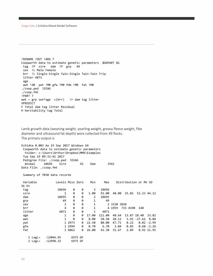
!RENAME !OUT !ARG 7 Coopworth data to estimate genetic parameters $DOPART $1 tag !P sire dam !P grp 49 sex !L Male Female brr !L Single-Single Twin-Single Twin-Twin Trip litter 4871 age wwt !d0 ywt !M0 gfw !M0 fdm !M0 fat !M0 ./coop.ped !DIAG ./coop.fmt !PART 7 wwt ~ grp sex*age c(brr) !r dam tag litter VPREDICT F Total dam tag litter Residual H heritability tag Total
Lamb growth data (weaning weight, yearling weight, greasy fleece weight, fibe diameter and ultrasound fat depth) were collected from 49 flocks. The primary output is
Echidna 0.003 Aa 19 Sep 2017 Windows 64 Coopworth data to estimate genetic parameters Folder: c:\Users\Arthur\Dropbox\MMX\Examples Tue Sep 19 09:33:41 2017 Pedigree File: ./coop.ped !DIAG Animal 10696 Sire 92 Dam 3561 Data File: ./coop.fmt Summary of 7030 data records Variable Levels Miss Zero Min Max Distribution or Mn SD Sk Kt tag 10696 0 0 3 10696 sire 1 0 0 1.00 92.00 48.00 25.02 52.23 44.12 dam 10695 0 0 2 10695 grp 49 0 0 1 49 sex 2 0 0 1 2 3220 3810 brr 4 0 0 1 4 1959 733 4190 148 litter 4871 0 0 1 4871 age 1 0 0 17.00 111.00 48.64 13.87 18.40 33.82 wwt 1 0 0 8.00 50.50 28.12 5.92 -27.62 8.04 ywt 1 2973 0 22.50 80.00 47.71 8.22 0.02 -2.99 gfw 1 2994 0 0.70 6.70 3.04 0.85 0.60 -2.26 fat 1 6062 0 26.00 41.30 31.67 2.89 8.92 11.95 1 LogL= -13044.95 6975 DF 2 LogL= -12998.32 6975 DF

Cargo Vale | Echidna Mixed Model Software
34
3 LogL= -12993.96 6975 DF 4 LogL= -12993.81 6975 DF 5 LogL= -12993.80 6975 DF Analysis of wwt Wald F statistics Source of Variation NumDF DenDF F-inc P-inc grp 49 1547.04 sex 1 680.59 age 1 1063.79 sex.age 1 8.50 c(brr) 3 546.14 Model_Term Order Gamma Sigma Z_ratio %C dam 10695 0.184505 1.52007 3.88 0 P tag 10696 0.303631 2.50151 3.72 0 P litter 4871 0.467913 3.85496 8.93 0 P Residual_units 7030 1.00000 8.23863 18.68 0 dam 10695 effects fitted tag 10696 effects fitted litter 4871 effects fitted Finished: Tue Sep 19 09:33:46 2017 LogL Converged sped7/sped
Standard Spatial Analysis – Slate Hall Farm This wheat experiment tested 25 varieties in 6 replicates using a balanced incomplete
block design. Two standard models are shown in the code:
!REN !OUT !ARG 1 2 !DEB !LOG Slate Hall 1976 Cereal trial !DOPART $1 rep 6 latrow 30 latcol 30 fldrow 10 fldcol 15 variety 25 yield 1 !/10 weight !=V0 !== 145 !*-0.5 !+1 data\shf.dat !DISPLAY 15 !PART 1 # Balanced Incomplete Block Analysis yield ~ mu variety !r rep latrow latcol !PART 2 # AR1 x AR1 Spatial Analysis yield ~ mu variety residual ar1(fldrow):ar1(fldcol) !PART 1 2 PREDICT variety

Cargo Vale | Echidna Mixed Model Software
35
Output from part 1 Summary of 150 data records Variable Levels Miss Zero Min Max Distribution or Mn SD Sk Kt rep 6 0 0 1 6 25 25 25 25 25 25 latrow 30 0 0 1 30 latcol 30 0 0 1 30 fldrow 10 0 0 1 10 15 15 15 15 15 15 15 15 15 15 fldcol 15 0 0 1 15 variety 25 0 0 1 25 yield 1 0 0 91.70 211.90 147.04 23.23 63.90 187.08 1 LogL= -446.36 125 DF 2 LogL= -428.12 125 DF 3 LogL= -420.52 125 DF 4 LogL= -419.97 125 DF 5 LogL= -419.96 125 DF 6 LogL= -419.96 125 DF Analysis of yield Wald F statistics Source of Variation NumDF DenDF F-inc P-inc mu 1 1216.30 variety 24 8.84 Model_Term Order Gamma Sigma Z_ratio %C rep 6 0.528714 42.6239 0.62 0 P latrow 30 1.93444 155.951 3.06 0 P latcol 30 1.83725 148.115 3.04 0 P Residual_units 150 1.00000 80.6180 6.01 0 rep 6 effects fitted latrow 30 effects fitted latcol 30 effects fitted Finished: Tue Sep 26 09:05:23 2017 LogL Converged shf30/shf Echidna creates a residual plot for each analysis. It typically includes a plot of residuals against fitted values. In the case of a spatial analysis, it includes a heat map and a variogram. The plot from this analysis is

Cargo Vale | Echidna Mixed Model Software
36
In the heatmap, BLUE highlights the low plots (large negative residuals) and RED highlights the high plots (large positive residuals). The Variogram shows the variance of the difference between residuals separated distances in the two spatial directions. See Gilmour et al 1997 for a discussion on the use of variograms to elucidate spatial structure in residuals. Output from part 2 6 LogL= -412.50 125 DF Analysis of yield Wald F statistics Source of Variation NumDF DenDF F-inc P-inc mu 1 851.32 variety 24 13.04 Model_Term Order Gamma Sigma Z_ratio %C ar1(fldrow).ar1(fldcol) 150 effects ar1(fldrow) 10 0.458558 177.683 2151.60 0 P ar1(fldcol) 15 0.683772 264.949 4185.87 0 P Residual_units 150 1.00000 387.481 5.00 0 Finished: Tue Sep 26 09:24:58 2017 LogL Converged shf31/shf
Note that the spatial model has a better fit (LogL 7.46 higher with 1 less variance
parameter).
Residuals vs Fitted Values
ar1(fldrow_a).ar1(fldcol_b)
Range Plot

Cargo Vale | Echidna Mixed Model Software
37
Missing values in the spatial grid A second example is the Nebraska Interstate trial (see ningrid.es) which had 56 varieties
grown with 4 reps in a 22 x 11 grid. However, there is no data for 18 of the 442 grid
points. That is, the data file nin89.asd has only 242 rows of data.
If the model term mv is specified in the model, and a spatial residual model is
requested, Echidna will complete the grid so the spatial model can be fitted, estimating
18 missing values. Note that the model associated with the missing values is arbitrary
so that the missing value estimates are not useful. You could of course manually
complete the grid (so all plots are represented in the data) and then the missing value
estimates may be meaningful.
Basic Multi-environment trial
This is an unreplicated trial run at three locations. Six check varieties are sown on a
diagonal grid to give basic replication and allow estimation of spatial correlation.
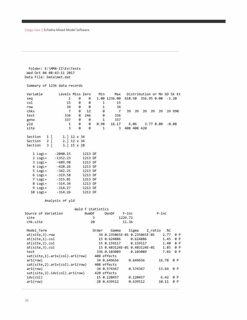
!DEB !LOG !OUT !RE !ARG 1 met test run !DOPART $1 seq col 15 # Actually 12 12 and 15 for the sites respectively row 34 # Actually 34 34 and 28 for the sites respectively chks 7 test 336 geno 337 yld 1 !*.01 site 3 Data\met.dat # !section site !ROW row !COL col !PART 1 yld ~ site chk.site !r at(site,3).row .02 at(site).col .036 .40 .9 test residual sat(site,3).idv(col).ar1(row) sat(site,2,1).ar1v(col).ar1(row) !PART 2 yld ~ site chk.site !r at(site,3).row .623 at(site).col test .103 residual sat(site,3).idv(col 0.12).ar1(row 0.64) sat(site,2,1).ar1v(col 0.195 .99).ar1(row 0.65)
Echidna 0.005 Aa 04 Oct 2017 Windows 64 met test run
Cargo Vale | Echidna Mixed Model Software
38
Folder: E:\MMX-II\Ex\Tests Wed Oct 04 08:43:11 2017 Data File: Data\met.dat Summary of 1236 data records Variable Levels Miss Zero Min Max Distribution or Mn SD Sk Kt seq 1 0 0 1.00 1236.00 618.50 356.95 0.00 -1.20 col 15 0 0 1 15 row 34 0 0 1 34 chks 7 0 12 0 7 39 39 39 39 39 39 990 test 336 0 246 0 336 geno 337 0 0 1 337 yld 1 0 0 0.98 16.17 6.06 3.77 0.80 -0.88 site 3 0 0 1 3 408 408 420 Section 1 [ 1.] 12 x 34 Section 2 [ 2.] 12 x 34 Section 3 [ 3.] 15 x 28 1 LogL= -2040.15 1213 DF 2 LogL= -1352.23 1213 DF 3 LogL= -689.98 1213 DF 4 LogL= -428.26 1213 DF 5 LogL= -342.25 1213 DF 6 LogL= -319.58 1213 DF 7 LogL= -315.01 1213 DF 8 LogL= -314.34 1213 DF 9 LogL= -314.27 1213 DF 10 LogL= -314.26 1213 DF Analysis of yld Wald F statistics Source of Variation NumDF DenDF F-inc P-inc site 3 1229.72 chk.site 20 11.36 Model_Term Order Gamma Sigma Z_ratio %C at(site,3).row 34 0.235065E-01 0.235065E-01 2.77 0 P at(site,1).col 15 0.624886 0.624886 1.45 0 P at(site,2).col 15 0.159117 0.159117 1.40 0 P at(site,3).col 15 0.483124E-01 0.483124E-01 1.85 0 P test 336 0.103089 0.103089 7.02 0 P sat(site,1).ar1v(col).ar1(row) 408 effects ar1(row) 34 0.649656 0.649656 16.78 0 P sat(site,2).ar1v(col).ar1(row) 408 effects ar1(row) 34 0.574367 0.574367 13.64 0 P sat(site,3).idv(col).ar1(row) 420 effects idv(col) 15 0.120457 0.120457 6.42 0 P ar1(row) 28 0.639512 0.639512 10.11 0 P

Cargo Vale | Echidna Mixed Model Software
39
at(site,3).row 34 effects fitted, 6 were zero. at(site,1).col 15 effects fitted. at(site,2).col 15 effects fitted. at(site,3).col 15 effects fitted. test 336 effects fitted, 18 were zero. Finished: Wed Oct 04 08:43:13 2017 LogL Converged met1/met
Multi-environment trial with six locations
This is a replicated trial testing 37 varieties at six locations. We demonstrate several
forms of the Factor analytic model to model the genetic covariance across sites. The
factor analytic model parameterizes the 6x6 variance matrix as ΓΓ’+Ψ where Γ here has
6 rows and 1 or 2 columns, Ψ is a diagonal matrix of order 6 of specific variances.
Specific variances may be zero (or negative). Spatial variation is modelled.
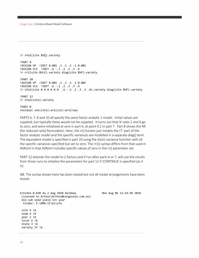
!WORK 1 !ren !ARG 12 !OUT !CONTINUE mid sub seed yield 1st year !DOPART $1 seq site 6 !A snam 6 !A year 2 !A locat 6 !A state 3 !A sy row 27 col 6 variety 37 !A lr lc species 14 !A sqrtsy logsy mssy.asd !skip 1 !maxit 22 !SLN !EXTRA 1 !PART 0 logsy ~ site site/c(species) mv, at(site,3).lr at(site,4).lr, !r at(site,1).col .13 at(site,5).col .39, at(site,6).col .05, !PART 6 !ASSIGN VQ !INIT 0 .1 .1 .1 .1 0 .6 -.1 .2 .3 .3 .4 !r xfa1(site $VQ).variety !PART 7 !ASSIGN VQ !INIT 0.001 .1 .1 .1 .1 0.001 .6 -.1 .2 .3 .3 .4
Cargo Vale | Echidna Mixed Model Software
40
!r xfa1(site $VQ).variety !PART 8 !ASSIGN VP !INIT 0.001 .1 .1 .1 .1 0.001 !ASSIGN VLE !INIT .6 -.1 .2 .3 .3 .4 !r rr1(site $VLE).variety diag(site $VP).variety !PART 10 !ASSIGN VP !INIT 0.001 .1 .1 .1 .1 0.001 !ASSIGN VLE !INIT .6 -.1 .2 .3 .3 .4 !r xfa1(site 0 0 0 0 0 0 .6 -.1 .2 .3 .3 .4).variety diag(site $VP).variety !PART 12 !r xfa2(site).variety !PART 0 residual sat(site):ar1(col):ar1(row)
PARTS 6, 7, 8 and 10 all specify the same factor analytic 1 model. Initial values are supplied, but typically these would not be supplied. It turns out that Ψ vales 1 and 6 go to zero, and were initialized at zero in part 6, at point 0.1 in part 7. Part 8 shows the RR (for reduced rank) formulation. Here, the rr() fuction just models the ΓΓ’ part of the factor analytic model and the specific variances are modelled in a separate diag() term. The equivalent model is specified in part 10 using the xfa1() variance function with all the specific variances specified but set to zero. The rr1() syntax differs from that used in ASReml in that ASReml includes specific values of zero in the rr() parameter set. PART 12 extends the model to 2 factors and if run after parts 6 or 7, will use the results from those runs to initialize the parameters for part 12 if !CONTINUE is specified (as it is). NB. The syntax shown here has been tested but not all model arrangements have been tested. Echidna 0.030 Aa 2 Aug 2018 Windows Mon Aug 06 12:24:30 2018 Licensed to Arthur([email protected]) mid sub seed yield 1st year Folder: E:\MMX-II\Ex\xfa site 6 !A snam 6 !A year 2 !A locat 6 !A state 3 !A variety 37 !A

Cargo Vale | Echidna Mixed Model Software
41
species 14 !A Data File: mssy.asd Summary of 535 data records Variable Levels Miss Zero Min Max Distribution or Mn SD Sk Kt seq 1 0 0 1.00 535.00 268.00 154.58 0.00 -1.21 site 6 0 0 1 6 104 104 66 66 81 114 snam 6 0 0 1 6 104 104 66 66 81 114 year 2 0 0 1 1 535 locat 6 0 0 1 6 104 104 66 66 81 114 state 3 0 0 1 3 322 132 81 sy 1 4 0 8.00 2331.00 301.02 203.53 2.68 18.78 row 27 0 0 1 27 col 6 0 0 1 6 120 120 120 93 41 41 variety 37 0 0 1 37 lr 1 0 21 -13.00 13.00 0.00 6.32 0.00 -0.75 lc 1 0 27 -2.50 2.50 0.00 1.39 0.00 -0.89 species 14 0 0 1 14 sqrtsy 1 1 1 0.00 48.28 16.39 5.55 0.44 1.85 logsy 1 4 0 2.19723 7.75448 5.48574 0.73733 -1.03 2.30 Warning: Unknown QUALIFIER NOD ignored in line: mssy.asd Warning: site_b taken as site Section 1 [ 1.] 4 x 26 Section 2 [ 2.] 4 x 26 Section 3 [ 3.] 6 x 11 Section 4 [ 4.] 6 x 11 Section 6 [ 6.] 6 x 19 sat(site,6).ar1(col).ar1(row) 1 LogL= -61.36 505 DF 2 LogL= -25.33 505 DF 3 LogL= 7.56 505 DF 4 LogL= 13.54 505 DF 5 LogL= 14.02 505 DF 6 LogL= 14.03 505 DF 7 LogL= 14.03 505 DF Analysis of logsy Wald F statistics Source of Variation NumDF DenDF F-inc P-inc site 6 2455.17 site.c(species) 18 4.56 Model_Term Order Gamma Sigma Z_ratio %C at(site,1).col 6 0.130346 0.130346 0.94 0 P at(site,5).col 6 0.389531 0.389531 0.98 0 P at(site,6).col 6 0.457810E-01 0.457810E-01 0.92 0 P xfa1(site_b).variety 259 effects xfa1(site_b) 0 1 7 0.00000 0.00000 0.00 0 F xfa1(site_b) 0 2 7 0.128853E-01 0.128853E-01 0.98 0 P xfa1(site_b) 0 3 7 0.830662E-02 0.830662E-02 0.20 -1 P

Cargo Vale | Echidna Mixed Model Software
42
xfa1(site_b) 0 4 7 0.855346E-01 0.855346E-01 1.55 0 P xfa1(site_b) 0 5 7 0.705927E-01 0.705927E-01 1.51 0 P xfa1(site_b) 0 6 7 0.00000 0.00000 0.00 0 F xfa1(site_b) 1 1 7 0.206451 0.206451 2.62 0 P xfa1(site_b) 1 2 7-0.251937E-01-0.251937E-01 -0.51 0 P xfa1(site_b) 1 3 7 0.189174 0.189174 2.17 0 P xfa1(site_b) 1 4 7 0.254406E-01 0.254406E-01 0.25 0 P xfa1(site_b) 1 5 7 0.169110E-01 0.169110E-01 0.16 2 P xfa1(site_b) 1 6 7 0.438153 0.438153 4.59 0 P sat(site,1).ar1(col).ar1(row) 104 effects ar1(col) 4 0.506758E-01 0.506758E-01 0.36 0 P ar1(row) 26 0.383241 0.383241 3.70 0 P ar1(row) 26 0.475011 0.475011 5.64 0 P sat(site,2).ar1(col).ar1(row) 104 effects ar1(col) 4 0.253246 0.253246 2.00 0 P ar1(row) 26 0.296927 0.296927 3.08 0 P ar1(row) 26 0.153510 0.153510 5.91 0 P sat(site,3).ar1(col).ar1(row) 66 effects ar1(col) 6 0.569952E-01 0.569952E-01 0.37 0 P ar1(row) 11 0.241967E-01 0.241967E-01 0.17 -1 P ar1(row) 11 0.279422 0.279422 4.58 0 P sat(site,4).ar1(col).ar1(row) 66 effects ar1(col) 6 0.236058 0.236058 1.42 0 P ar1(row) 11 0.460897 0.460897 3.14 0 P ar1(row) 11 0.377468 0.377468 3.81 0 P sat(site,5).ar1(col).ar1(row) 81 effects ar1(col) 3 0.240395 0.240395 1.51 0 P ar1(row) 27 0.758894E-02 0.758894E-02 0.06 0 P ar1(row) 27 0.289851 0.289851 5.32 0 P sat(site,6).ar1(col).ar1(row) 114 effects ar1(col) 6 0.192688 0.192688 1.46 0 P ar1(row) 19 0.301040 0.301040 2.46 0 P ar1(row) 19 0.311971 0.311971 5.44 0 P mv 4 effects fitted. at(site,3).lr 1 effects fitted. at(site,4).lr 1 effects fitted. at(site,1).col 6 effects fitted, 2 were zero. at(site,5).col 6 effects fitted, 3 were zero. at(site,6).col 6 effects fitted. xfa1(site_b).variety 259 effects fitted. Finished: Mon Aug 06 12:24:30 2018 LogL Converged mfa6/mfa
Lupin Multi-environment trial with 87 locations
This is an analysis of variety means from 87 lupin trials. There are 2019 means
representing 203 varieties (means in 11.4% of the two-way table). We have fitted

Cargo Vale | Echidna Mixed Model Software
43
models with 1, 2, 3 and 4 factors, and compare the loglikelihood with the results
obtained from ASReml 4.2.
!WORK 1 !ren !ARG 12 !OUT !CONTINUE !WORK 1 !RENAME !arg 1 2 2 3 3 4 !CON !OUT Title: ALBUS_2stage. !DOPART $1 #trial,year,region,variety,yield,rep,weight,ems #KFA02BURU,2002,NSW,KIEV-MUTANT,0.873,3,2136.562,0.0010000 trial !A year !I region !A variety !A yield rep * Weight ems weight !=Weight !*0.025 ALBUS.csv !SKIP 1 !MAXIT 50 !CONTINUE !PART 1 2 3 4 yield !wt=weight !DISP 0.025 ~ mu trial !r xfa$1(trial).var # ASR 2910.82 3017. 3158.34 3238.32 # Echidna 2910.37 3007 3157 3220.4 # 2911.47 3044 3221.15
The exact likelihood sequence is dependent on some tuning parameters built into the code and these will probably be changed. The xfa1() model reports a Log Likelihood of 2911.47. This model includes 10 specific variances of zero. Progressing to xfa2() increases the likelihood to 3044 (after a CONTINUE), a gain of 133, and has 24 specific variances of zero. This gain is associated with 72 (87 -1 -14) extra free parameters. The xfa3() model increases the likelihood by 113 to 3157 and has 32 specific variances of zero. This gain is associated with 77 (87 -2 -8) extra free parameters. The gain from fitting xfa4 (whether 80 from ASReml, or 64 from Echidna) has 84/69 (87-3-15) free parameters. (The ASreml result only has 19 zero PSI). Echidna 0.030 Aa 2 Aug 2018 Windows Thu Aug 09 15:31:19 2018 Licensed to Arthur([email protected]) Title: ALBUS_2stage. Folder: E:\MMX-II\Ex\xfa trial !A year !I region !A variety !A ems weight !=Weight !*0.025 Data File: ALBUS.csv

Cargo Vale | Echidna Mixed Model Software
44
Summary of 2019 data records Variable Levels Miss Zero Min Max Distribution or Mn SD Sk Kt trial 87 0 0 1 87 year 5 0 0 1 5 337 438 518 430 296 region 3 0 0 1 3 1940 24 55 variety 203 0 0 1 203 yield 1 0 0 0.09 5.61 1.73 1.08 0.56 -0.50 rep 6 0 0 1 6 201 294 1485 18 6 15 Weight 1 0 0 8. 13415. 590. 1131. 4.84 29.70 ems 1 0 0 0.00037 0.39100 0.02491 0.04671 5.95 42.38 weight 1 0 0 0.19 335.37 14.75 28.27 4.84 29.70 Notice: Updating initial parameter values from .esv file if present. Notice: 26 variance parameter constraint codes were changed when reading the .esv file! 1 LogL= 3008.94 1932 DF 2 LogL= 3009.65 1932 DF 3 LogL= 3010.68 1932 DF 4 LogL= 3011.40 1932 DF 5 LogL= 3012.48 1932 DF 6 LogL= 3013.27 1932 DF 7 LogL= 3014.46 1932 DF 8 LogL= 3015.38 1932 DF 9 LogL= 3016.36 1932 DF 10 LogL= 3017.42 1932 DF 11 LogL= 3018.56 1932 DF 12 LogL= 3019.78 1932 DF 13 LogL= 3020.98 1932 DF 14 LogL= 3022.95 1932 DF 15 LogL= 3024.63 1932 DF 16 LogL= 3026.20 1932 DF 17 LogL= 3027.65 1932 DF 18 LogL= 3028.96 1932 DF 19 LogL= 3030.12 1932 DF 20 LogL= 3031.15 1932 DF 21 LogL= 3032.03 1932 DF 22 LogL= 3033.13 1932 DF 23 LogL= 3033.72 1932 DF 24 LogL= 3034.40 1932 DF 25 LogL= 3034.89 1932 DF 26 LogL= 3035.27 1932 DF 27 LogL= 3035.71 1932 DF 28 LogL= 3036.10 1932 DF 29 LogL= 3036.51 1932 DF 30 LogL= 3036.97 1932 DF 31 LogL= 3037.55 1932 DF 32 LogL= 3038.47 1932 DF 33 LogL= 3039.53 1932 DF 34 LogL= 3040.63 1932 DF

Cargo Vale | Echidna Mixed Model Software
45
35 LogL= 3041.35 1932 DF 36 LogL= 3042.02 1932 DF 37 LogL= 3042.44 1932 DF 38 LogL= 3042.78 1932 DF 39 LogL= 3043.05 1932 DF 40 LogL= 3043.28 1932 DF 41 LogL= 3043.48 1932 DF 42 LogL= 3043.65 1932 DF 43 LogL= 3043.79 1932 DF 44 LogL= 3043.94 1932 DF 45 LogL= 3044.06 1932 DF 46 LogL= 3044.16 1932 DF 47 LogL= 3044.24 1932 DF 48 LogL= 3044.31 1932 DF 49 LogL= 3044.38 1932 DF 50 LogL= 3044.44 1932 DF Analysis of yield Wald F statistics Source of Variation NumDF DenDF F-inc P-inc mu 1 61146.84 trial 86 1244.24 Model_Term Order Gamma Sigma Z_ratio %C xfa2(trial).var 18067 effects xfa2(trial) 0 1 89 0.560555E-02 0.560555E-02 3.02 0 P xfa2(trial) 0 2 89 0.436437E-02 0.436437E-02 1.16 0 P xfa2(trial) 0 3 89 0.171608E-02 0.171608E-02 2.06 0 P xfa2(trial) 0 4 89 0.297772E-02 0.297772E-02 2.54 0 P xfa2(trial) 0 5 89 0.00000 0.00000 0.00 0 F xfa2(trial) 0 6 89 0.00000 0.00000 0.00 0 F xfa2(trial) 0 7 89 0.100567E-02 0.100567E-02 1.54 0 P …
Simple multivariate analysis A wether trial conducted at Orange, NSW recorded … for wethers grouped in teams
representing various bloodlines. The basic multivariate analysis is coded as
!DEBUG !LOG !OUT !ARG 6 !RENAME ORANGE WETHER TRIAL 84-88 !DOPART $1 TAG TEAM 35 YEAR 2 GFW YLD FDIAM Data/orangeWetherTrial.dat !FORMAT(I4,6X,I3,I2,3F4.1)

Cargo Vale | Echidna Mixed Model Software
46
!PART 6 !ASSIGN VTeam .4 .4 1.14 !ASSIGN Verror .4 .4 2.2 GFW FDIAM ~ Trait Tr.c(YEAR) !r us(Tr_a).TEAM traits.team residual units:us(Trait_b)
The FORMAT statement is used because this old data was prepared without delimitors,
looking like
0101 3 21 1 1 56 743 185
0101 3 21 1 2 60 712 196
0101 3 21 1 3 80 757 215
Is read as
0101 1 1 5.6 74.3 18.5
0101 1 2 6.0 71.2 19.6
0101 1 3 8.0 75.7 21.5
Note the use of the !ASSIGN statements to supply initial values for the two us structures. If the model was written without the ASSIGN statements, as GFW FDIAM ~ Trait Tr.c(YEAR) !r us(Tr .4 .4 1.14).TEAM traits.team residual units:us(Trait .4 .4 2.2) Echidna would move the start values into ASSIGN strings anyway, while parsing the
model.
Echidna 0.006 Aa 19 Oct 2017 Windows 64 ORANGE WETHER TRIAL 84-88 Folder: E:\MMX-II\Ex\Tests Thu Oct 19 11:25:10 2017 Data File: Data/orangeWetherTrial.dat Summary of 1485 data records Variable Levels Miss Zero Min Max Distribution or Mn SD Sk Kt TAG 1 0 0 101. 4015. 2060. 1130. 0.06 -1.13 TEAM 35 0 0 1 35 YEAR 3 0 0 1 3 455 517 513 GFW 1 0 0 4.10 11.20 7.48 1.05 0.28 0.11 YLD 1 0 0 60.30 88.60 75.11 4.38 -0.22 -0.01 FDIAM 1 0 0 15.90 30.60 22.29 2.19 0.19 -0.10 Warning: Tr_b taken as Trait 1 LogL= -1529.20 2964 DF 2 LogL= -1521.48 2964 DF 3 LogL= -1507.61 2964 DF 4 LogL= -1503.82 2964 DF

Cargo Vale | Echidna Mixed Model Software
47
5 LogL= -1503.62 2964 DF 6 LogL= -1503.62 2964 DF Analysis of GFW FDIAM Wald F statistics Source of Variation NumDF DenDF F-inc P-inc Trait 2 5920.13 Tr.c(YEAR) 4 354.40 Model_Term Order Gamma Sigma Z_ratio %C us(Tr_b).TEAM 70 effects us(Tr_b) 2 0.387107 0.387107 4.02 0 P us(Tr_b) 2 0.400617 0.400617 2.67 0 P us(Tr_b) 2 1.44691 1.44691 3.98 0 P units.us(Trait_c) 2970 effects us(Trait_c) 2 0.444170 0.444170 26.91 0 P us(Trait_c) 2 0.352635 0.352635 12.76 0 P us(Trait_c) 2 2.20813 2.20813 26.91 0 P us(Tr_b).TEAM 70 effects fitted. Finished: Thu Oct 19 11:25:10 2017 LogL Converged owt1/owt
Bivariate animal model with missing observations Coopworth 12 Adding the model lines
!PART 12 // wwt ywt ~ Trait Tr.(grp sex age c(brr) ) + !r us(Tr 1.2 1.1 1.1).dam us(Tr 2.8 3 6.2).tag us(Tr 4 2.5 3).litter residual units.us(Trait 8 5 15) VPREDICT F Total dam tag litter units H heritability tag Total R R_g tag
to the Coopworth example and running it gives
Echidna 0.014 Aa 02 Nov 2017 Windows 64
wwt Weaning weight Pedigree Direct Genetic
Folder: E:\MMX-II\Ex\Tests
Thu Nov 02 14:56:37 2017
Pedigree File: ./coop.ped !DIAG
Animal 10696 Sire 92 Dam 3561
Data File: ./coop.fmt
Summary of 7030 data records
Variable Levels Miss Zero Min Max Distribution or Mn SD Sk Kt

Cargo Vale | Echidna Mixed Model Software
48
tag 10696 0 0 3 10696
sire 1 0 0 1.00 92.00 48.00 25.02 -0.25 -1.10
dam 10696 0 0 2 10695
grp 49 0 0 1 49
sex 2 0 0 1 2 3220 3810
brr 4 0 0 1 4 1959 733 4190 148
litter 4871 0 0 1 4871
age 1 0 0 17.00 111.00 48.64 13.87 0.93 1.40
wwt 1 0 0 8.00 50.50 28.12 5.92 0.17 -0.05
ywt 1 2973 0 22.50 80.00 47.71 8.22 0.24 -0.16
gfw 1 2994 0 0.70000 6.7000 3.039 0.84963 0.47 0.27
fat 1 6062 0 26.00 41.30 31.67 2.89 0.38 -0.09
Warning: Tr taken as Trait
Warning: Tr_a taken as Trait
Warning: Tr_b taken as Trait
Warning: Tr_c taken as Trait
1 LogL= -20684.80 10982 DF
2 LogL= -20683.81 10982 DF
3 LogL= -20682.70 10982 DF
4 LogL= -20682.69 10982 DF
5 LogL= -20682.69 10982 DF
Analysis of wwt ywt
Wald F statistics
Source of Variation NumDF DenDF F-inc P-inc
Trait 2 48085.45
Tr.grp 93 77.95
Tr.sex 2 1198.49
Tr.age 2 538.65
Tr.c(brr) 6 279.21
Model_Term Order Gamma Sigma Z_ratio %C
us(Tr_a).dam 21392 effects
us(Tr_a) 2 1.58551 1.58551 4.05 0 P
us(Tr_a) 2 1.50152 1.50152 3.11 0 P
us(Tr_a) 2 0.901185 0.901185 0.99 0 P
us(Tr_b).tag 21392 effects
us(Tr_b) 2 2.46311 2.46311 3.69 0 P
us(Tr_b) 2 2.74701 2.74701 3.14 0 P
us(Tr_b) 2 6.13120 6.13120 3.76 0 P
us(Tr_c).litter 9742 effects
us(Tr_c) 2 3.82504 3.82504 8.87 0 P
us(Tr_c) 2 2.30567 2.30567 4.36 0 P
us(Tr_c) 2 3.33782 3.33782 3.29 0 P
units.us(Trait_d) 14060 effects
us(Trait_d) 2 8.26037 8.26037 18.83 0 P
us(Trait_d) 2 5.52531 5.52531 9.59 0 P
us(Trait_d) 2 15.5937 15.5937 14.25 0 P
us(Tr_a).dam 21392 effects fitted, 82 were zero.
us(Tr_b).tag 21392 effects fitted, 82 were zero.
us(Tr_c).litter 9742 effects fitted, 34 were zero.
Finished: Thu Nov 02 14:58:53 2017 LogL Converged sped12/sped

Cargo Vale | Echidna Mixed Model Software
49
Notice that the dam matrix is not positive definite as that constraint has not been
implemented yet.
The VPREDICT statement produces an .epv file containing
us(Tr_a).dam 21392 effects fitted, 82 were zero.
1 Residual 1.0000 0.0000
2 us(Tr_c).litter;us(Tr_c) 3.8251 0.43111
3 us(Tr_c).litter;us(Tr_c) 2.3058 0.52919
4 us(Tr_c).litter;us(Tr_c) 3.3393 1.0154
5 us(Tr_b).tag;us(Tr_b) 2.4631 0.66667
6 us(Tr_b).tag;us(Tr_b) 2.7471 0.87510
7 us(Tr_b).tag;us(Tr_b) 6.1314 1.6305
8 us(Tr_a).dam;us(Tr_a) 1.5855 0.39143
9 us(Tr_a).dam;us(Tr_a) 1.5014 0.48210
10 us(Tr_a).dam;us(Tr_a) 0.89971 0.90802
11 units.us(Trait_d);us(Trait_d) 8.2604 0.43877
12 units.us(Trait_d);us(Trait_d) 5.5253 0.57641
13 units.us(Trait_d);us(Trait_d) 15.594 1.0944
14 Total 16.134 0.32056
15 Total 12.080 0.39522
16 Total 25.964 0.67721
heritability = us(Tr_b) 5/Total 14 = 0.15266 0.03996
heritability = us(Tr_b) 7/Total 16 = 0.23615 0.05951
R_g 2 1 = us(Tr 6/SQR[us(Tr 5*us(Tr 7]= 0.7069 0.1037
Notice: The parameter estimates are followed by
their approximate standard errors. us(Tr_b).tag
21392 effects fitted, 82 were zero.
GLMM Sire model for Lamb foot scoring data. M Alwan in a masters project at Messey University score the feet of 2513 lambs and the
results are summarized in the file lamb.dat. The lambs represented 18 sires in 5
groups. The aim of this analysis is to estimate the heritability on the liability scale.
!DEBUG !LOG !OUT !REN !ARG 1 Lamb data from ARG thesis page 177-8 !DOPART $1 CYR GRP 5 SEX SIRE !I TOT L5 !/TOT # Express as a proportion L4 LS LR lamb.dat !skip 1 !DDF -1 !PART 1 L5 !bin !TOTAL=TOT !DISP 1 ~ mu SEX GRP !r SIRE .16783 VPREDICT F Total Residual*3.289 + SIRE F Genetic SIRE*4 H Heritability Genetic Total
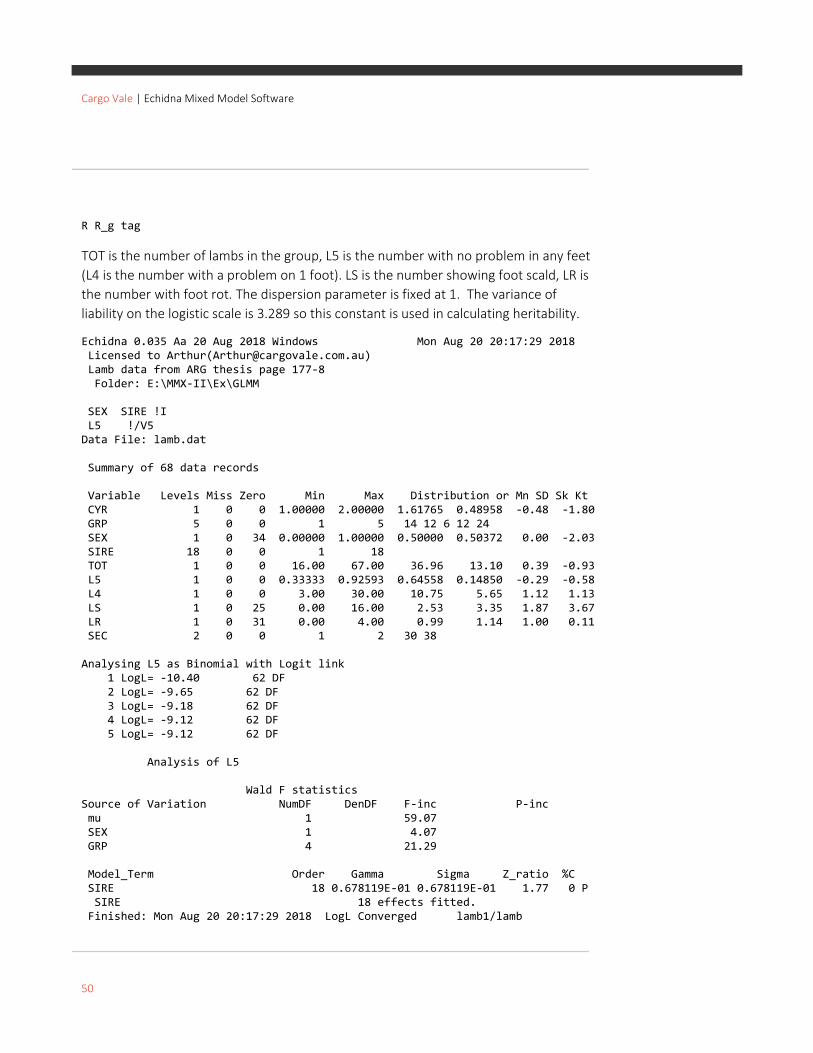
Cargo Vale | Echidna Mixed Model Software
50
R R_g tag
TOT is the number of lambs in the group, L5 is the number with no problem in any feet
(L4 is the number with a problem on 1 foot). LS is the number showing foot scald, LR is
the number with foot rot. The dispersion parameter is fixed at 1. The variance of
liability on the logistic scale is 3.289 so this constant is used in calculating heritability.
Echidna 0.035 Aa 20 Aug 2018 Windows Mon Aug 20 20:17:29 2018 Licensed to Arthur([email protected]) Lamb data from ARG thesis page 177-8 Folder: E:\MMX-II\Ex\GLMM SEX SIRE !I L5 !/V5 Data File: lamb.dat Summary of 68 data records Variable Levels Miss Zero Min Max Distribution or Mn SD Sk Kt CYR 1 0 0 1.00000 2.00000 1.61765 0.48958 -0.48 -1.80 GRP 5 0 0 1 5 14 12 6 12 24 SEX 1 0 34 0.00000 1.00000 0.50000 0.50372 0.00 -2.03 SIRE 18 0 0 1 18 TOT 1 0 0 16.00 67.00 36.96 13.10 0.39 -0.93 L5 1 0 0 0.33333 0.92593 0.64558 0.14850 -0.29 -0.58 L4 1 0 0 3.00 30.00 10.75 5.65 1.12 1.13 LS 1 0 25 0.00 16.00 2.53 3.35 1.87 3.67 LR 1 0 31 0.00 4.00 0.99 1.14 1.00 0.11 SEC 2 0 0 1 2 30 38 Analysing L5 as Binomial with Logit link 1 LogL= -10.40 62 DF 2 LogL= -9.65 62 DF 3 LogL= -9.18 62 DF 4 LogL= -9.12 62 DF 5 LogL= -9.12 62 DF Analysis of L5 Wald F statistics Source of Variation NumDF DenDF F-inc P-inc mu 1 59.07 SEX 1 4.07 GRP 4 21.29 Model_Term Order Gamma Sigma Z_ratio %C SIRE 18 0.678119E-01 0.678119E-01 1.77 0 P SIRE 18 effects fitted. Finished: Mon Aug 20 20:17:29 2018 LogL Converged lamb1/lamb

Cargo Vale | Echidna Mixed Model Software
51
The heritability is reported in the .evp file.
1 Residual 1.0000 0.0000 2 SIRE 0.67812E-01 0.38208E-01 3 Total 3.3568 0.38208E-01 4 Genetic 0.27125 0.15283 Heritability = Genetic 4/Total 3 = 0.08081 0.04461 Notice: The parameter estimates are followed by their approximate standard errors.
Figure produced from the Orange tree data by the command PLOT x circ !JOIN !VIEW
this is the orange data
x
circ
214.000
30.0000118.000 1582.00

Cargo Vale | Echidna Mixed Model Software
52
List of References
Gilmour, A.R., Anderson, R.D. and Rae, A.L. (1985). The analysis of binomial
data by a generalized linear mixed model. Biometrika, 72: 593 599.
http://dx.doi.org/10.1093/biomet/72.3.593
Gilmour, A.R., Luff, A.F., Fogarty, N.M. and Banks, R.G. (1994). Genetic
parameters for ultrasonic fat depth and eye muscle measurements in live Poll
Dorset sheep. Australian Journal of Agricultural Research, 45, 1281-91.
Gilmour, A.R., Thompson, R. and Cullis, B.R. (1995). Average Information
REML, an efficient algorithm for variance parameter estimation in linear
mixed models. Biometrics 51, 1440-50.
Gilmour, A.R., Cullis, B.R. and Verbyla, A. (1997). Accounting for Natural
and Extraneous Variation in the Analysis of Field Experiments. Journal of
Agricultural, Biological and Environmental Statistics 2, 269-293.


