
Lecture 14: Contingency Analysis,
Sensitivity Methods
ECEN 615Methods of Electric Power Systems Analysis
Prof. Tom Overbye
Dept. of Electrical and Computer Engineering
Texas A&M University

Announcements
• Homework 3 is due today
• Read Chapter 7 (the term reliability is now used instead
of security)
• Midterm exam is Oct 18 in class
• Off campus students should work with Iyke to get their exam
proctoring setup
• Closed book, closed notes, but calculators and one 8.5 by 11
inch note sheet allowed
• Exam covers up to the end of today’s lecture
• Book material is intended to be supplementary; nothing from
the book not covered in class or homework will be on the exam
2

Contingency Analysis
• Contingency analysis is the process of checking the
impact of statistically likely contingencies
– Example contingencies include the loss of a generator, the loss
of a transmission line or the loss of all transmission lines in a
common corridor
– Statistically likely contingencies can be quite involved, and
might include automatic or operator actions, such as switching
load
• Reliable power system operation requires that the
system be able to operate with no unacceptable
violations even when these contingencies occur
– N-1 reliable operation considers the loss of any single element
3

Contingency Analysis
• Of course this process can be automated with the usual
approach of first defining a contingency set, and then
sequentially applying the contingencies and checking
for violations
– This process can naturally be done in parallel
– Contingency sets can get quite large, especially if one
considers N-2 (outages of two elements) or N-1-1 (initial
outage, followed by adjustment, then second outage
• The assumption is usually most contingencies will not
cause problems, so screening methods can be used to
quickly eliminate many contingencies
– We’ll cover these later (Gabe Ejebe is NAE class of 2018)4

Contingency Analysis in PowerWorld
• Automated using the Contingency Analysis tool
5

Power System Control and Sensitivities
• A major issue with power system operation is the
limited capacity of the transmission system
– lines/transformers have limits (usually thermal)
– no direct way of controlling flow down a transmission line
(e.g., there are no valves to close to limit flow)
– open transmission system access associated with industry
restructuring is stressing the system in new ways
• We need to indirectly control transmission line flow by
changing the generator outputs
• Similar control issues with voltage
6

Indirect Transmission Line Control
• What we would like to determine is how a change
in generation at bus k affects the power flow on a
line from bus i to bus j.
The assumption is
that the change
in generation is
absorbed by the
slack bus
7
Power Flow Simulation - Before
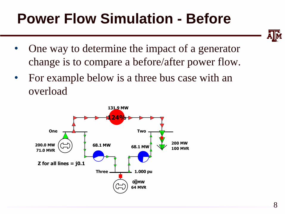
• One way to determine the impact of a generator
change is to compare a before/after power flow.
• For example below is a three bus case with an
overload
Z for all lines = j0.1
One Two
200 MW
100 MVR200.0 MW
71.0 MVR
Three 1.000 pu
0 MW
64 MVR
131.9 MW
68.1 MW 68.1 MW
124%
8

Power Flow Simulation - After
• Increasing the generation at bus 3 by 95 MW (and
hence decreasing it at bus 1 by a corresponding
amount), results in a 30.3 MW drop in the MW flow on
the line from bus 1 to 2, and a 64.7 MW drop
on the flow from 1 to 3.
Z for all lines = j0.1Limit for all lines = 150 MVA
One Two
200 MW
100 MVR105.0 MW
64.3 MVR
Three1.000 pu
95 MW
64 MVR
101.6 MW
3.4 MW 98.4 MW
92%
100% Expressed as a
percent, 30.3/95
=32% and
64.7/95=68%
9
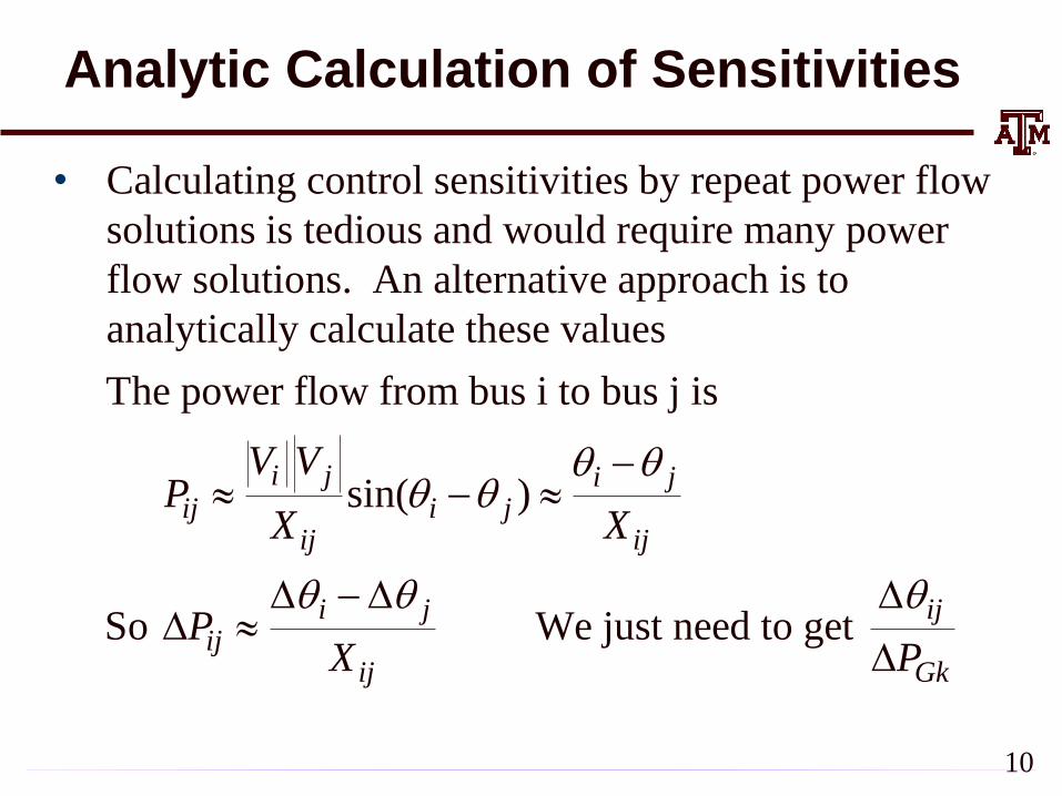
Analytic Calculation of Sensitivities
• Calculating control sensitivities by repeat power flow
solutions is tedious and would require many power
flow solutions. An alternative approach is to
analytically calculate these values
The power flow from bus i to bus j is
sin( )
So We just need to get
i j i jij i j
ij ij
i j ijij
ij Gk
V VP
X X
PX P
10

Analytic Sensitivities
1
From the fast decoupled power flow we know
( )
So to get the change in due to a change of
generation at bus k, just set ( ) equal to
all zeros except a minus one at position k.
0
1
0
θ B P x
θ
P x
P Bus k
11

Three Bus Sensitivity Example
line
bus
12
3
For a three bus, three line case with Z 0.1
20 10 1020 10
10 20 1010 20
10 10 20
Hence for a change of generation at bus 3
20 10 0 0.0333
10 20 1 0.0667
j
j
Y B
3 to 1
3 to 2 2 to 1
0.0667 0Then P 0.667 pu
0.1
P 0.333 pu P 0.333 pu
12

More General Sensitivity Analysis: Notation
• We consider a system with n buses and L lines given
by the set given by the set
– Some authors designate the slack as bus zero; an alternative
approach, that is easier to implement in cases with multiple
islands and hence slacks, is to allow any bus to be the slack,
and just set its associated equations to trivial equations just
stating that the slack bus voltage is constant
• We may denote the kth transmission line or transformer in the system, k , as
( , ),k k k
i j
from node to node
1 2{ , , , }
LL
13

Notation, cont.
• We’ll denote the real power flowing on k from bus i
to bus j as ƒk• The vector of real power flows on the L lines is:
which we simplify to
• The bus real and reactive power injection vectors are
1 2f [ , , , ]
L
Tf f f
1 2f [ , , , ]
T
Lf f f
1 2p [ , , , ]
TN
p p p
1 2q [ , , , ]
TN
q q q
14

Notation, cont.
• The series admittance of line is g +jb and we
define
• We define the LN incidence matrix
1 2B , , ,
Ldiag b b b
1
2
a
aA
aL
T
T
T
where the component j of ai isnonzero whenever line i is
coincident with node j. Hence
A is quite sparse, with two
nonzeros per row
15

Analysis Example: Available Transfer Capability
• The power system available transfer capability or
ATC is defined as the maximum additional MW
that can be transferred between two specific areas,
while meeting all the specified pre- and post-
contingency system conditions
• ATC impacts measurably the market outcomes and
system reliability and, therefore, the ATC values
impact the system and market behavior
• A useful reference on ATC is Available Transfer
Capability Definitions and Determination from
NERC, June 1996 (available freely online)
16
ATC and Its Key Components
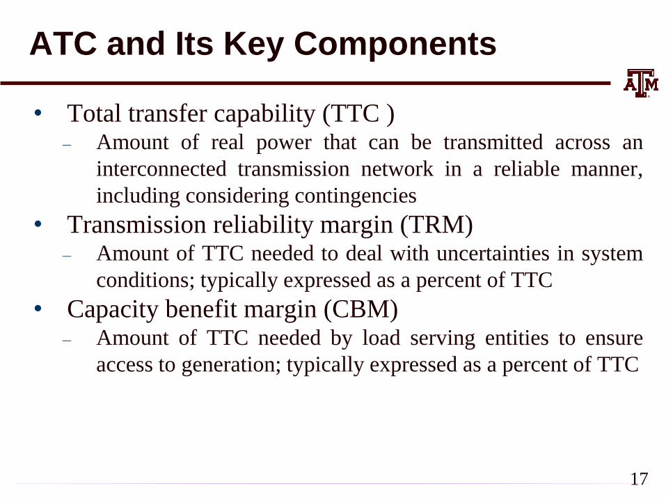
• Total transfer capability (TTC )– Amount of real power that can be transmitted across an
interconnected transmission network in a reliable manner,
including considering contingencies
• Transmission reliability margin (TRM)– Amount of TTC needed to deal with uncertainties in system
conditions; typically expressed as a percent of TTC
• Capacity benefit margin (CBM)– Amount of TTC needed by load serving entities to ensure
access to generation; typically expressed as a percent of TTC
17

ATC and Its Key Components
• Uncommitted transfer capability (UTC)UTC TTC – existing transmission commitment
• Formal definition of ATC isATC UTC – CBM – TRM
• We focus on determining Um,n, the UTC from node m
to node n
• Um,n is defined as the maximum additional MW that
can be transferred from node m to node n without
violating any limit in either the base case or in any post-
contingency conditions
18

UTC (or TTC) Evaluation
nm
t t
maxf
i j
no
limit
violation
,
( )
. .
m n
j max
U = max t
s t
f f f
L
for the base case j = 0 and each contingency case
j = 1,2 … , J
( )0f f
19
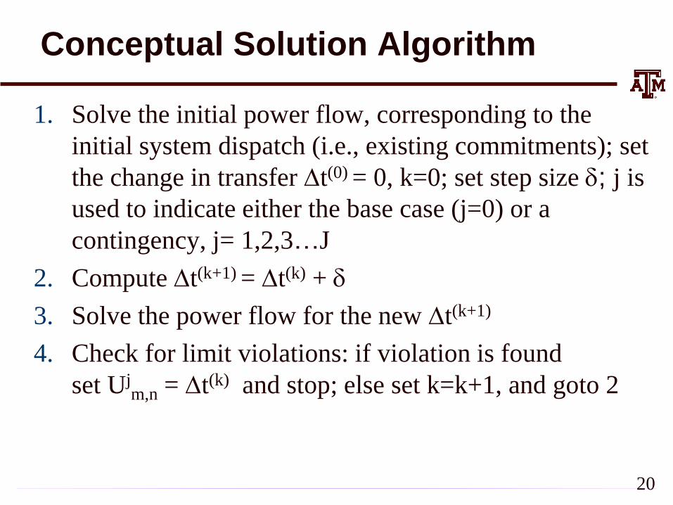
Conceptual Solution Algorithm
1. Solve the initial power flow, corresponding to the
initial system dispatch (i.e., existing commitments); set
the change in transfer t(0) = 0, k=0; set step size d; j is
used to indicate either the base case (j=0) or a
contingency, j= 1,2,3…J
2. Compute t(k+1) = t(k) + d
3. Solve the power flow for the new t(k+1)
4. Check for limit violations: if violation is found
set Ujm,n = t(k) and stop; else set k=k+1, and goto 2
20

Conceptual Solution Algorithm, cont.
• This algorithm is applied for the base case (j=0) and
each specified contingency case, j=1,2,..J
• The final UTC, Um,n is then determined by
• This algorithm can be easily performed on parallel
processors since each contingency evaluation is
independent of the other
( )
, ,
j
m n m n0 j J
U = min U
21

Five Bus Example: Reference
Line 1
Line 2
Line 3
Line 6
Line 5
Line 4slack
1.050 pu
42 MW
67 MW
100 MW
118 MW
1.040 pu
1.042 pu
A
MVA
A
MVA
A
MVA
1.042 pu
A
MVA
1.044 pu
33 MW
MW200
258 MW
MW118
260 MW
100 MW
MW100
A
MVA
One Two
Three
Four
Five
PowerWorld Case: B5_DistFact 22

Five Bus Example: Reference
3
( MW )
1 2 0 6.25 150
1 3 0 12.5 400
1 4 0 12.5 150
2 3 0 12.5 150
3 4 0 12.5 150
4 5 0 10 1,000
i j g b maxf
1
2
4
5
6
23

5 - BUS SYSTEM EXAMPLE
• We evaluate U2,3 using the previous procedure– Gradually increase generation at Bus 2 and load at Bus 3
• We consider the base case and the single contingency
with line 2 outaged (between 1 and 3): J 1
• Simulation results show for the base case that
• And for the contingency that
• Hence ( ) (1)
2,3 2,3 2,3, 24
0U min U U MW
( )
2,345
0U MW
(1)
2,324U MW
24

Five Bus: Maximum Base Case Transfer
Line 1
Line 2
Line 3
Line 6
Line 5
Line 4slack
1.050 pu
55 MW
71 MW
100 MW
150 MW
1.040 pu
1.041 pu
A
MVA
A
MVA
1.041 pu
A
MVA
1.043 pu
29 MW
MW200
258 MW
MW163
305 MW
100 MW
MW100
A
MVA
One Two
Three
Four
Five
100%A
MVA
2,3
( )45
0U MW
25

Five Bus: Maximum Contingency Transfer
Line 1
Line 2
Line 3
Line 6
Line 5
Line 4slack
1.050 pu
34 MW
92 MW
100 MW
150 MW
1.040 pu
1.036 pu
A
MVA
A
MVA
1.038 pu
A
MVA
1.040 pu
8 MW
MW200
258 MW
MW142
284 MW
100 MW
MW100
One Two
Three
Four
Five
100%A
MVA
2,3
(1)24U MW
26

Computational Considerations
• Obviously such a brute force approach can run into
computational issues with large systems
• Consider the following situation:– 10 iterations for each case
– 6,000 contingencies
– 2 seconds to solve each power flow
• It will take over 33 hours to compute a single UTC
for the specified transfer direction from m to n.
• Consequently, there is an acute need to develop fast
tools that can provide satisfactory estimates
27

Problem Formulation
• Denote the system state by
• Denote the conditions corresponding to the existing
commitment/dispatch by s(0), p(0) and f(0) so that
θx
V
1 2θ [ , , , ]
N T
1 2V [ , , , ]
N TV V V
( ) ( )
( ) ( )
g(x ,p ) 0
f h(x )
0 0
0 0
the power flow equations
line real power flow vector
28

Problem Formulation
1
( , )N
P k m k m k m k
k k m k m
m
g s p V V G cos B sin p
2
( ) ( ) ( ), ,i i j i j i j i j
h s g V V V cos b V V sin i j
g (x,p)g(x,p)
g (x,p)
P
Q
1
( , )N
Q m m k m k m k
k k m k m
m
g s p V V G sin B cos q
29
g includes the real and reactive
power balance equations

Problem Formulation
• For a small change, p, that moves the injection
from p(0) to p(0) + p , we have a corresponding
change in the state x with
• We then apply a first order Taylor’s series expansion
( ) ( )g (x x, p) 0
0 0p
( ) ( )
( ) ( )
( ) ( ) ( ) ( )
x p
x p
gg x x,p p g x ,p x
x
g. . .
p
0 0
0 0
0 0 0 0
p h o t
30

Problem Formulation
• We consider this to be a “small signal” change, so we
can neglect the higher order terms (h.o.t.) in the
expansion
• Hence we should still be satisfying the power balance
equations with this perturbation; so
( ) ( ) ( ) ( )x p x p
g gx 0
x p0 0 0 0
p
31

Problem Formulation
• Also, from the power flow equations, we obtain
g
p Ig
0p g
p
P
Q
g g
g θ VJ(x,p)
x g g
θ V
P P
Q Q
and then just the power flow Jacobian
32

Problem Formulation
• With the standard assumption that the power flow
Jacobian is nonsingular, then
• We can then compute the change in the line real
power flow vector
0 01
( ) ( )I
x J(x ,p ) p0
1( ) ( )
Ih hf s (x ,p ) p
x x 0
T T
0 0J
33

Sensitivity Comments
• Sensitivities can easily be calculated even for large
systems
– If p is sparse (just a few injections) then we can use a fast
forward; if sensitivities on a subset of lines are desired we
could also use a fast backward
• Sensitivities are dependent upon the operating point
– They also include the impact of marginal losses
• Sensitivities could easily be expanded to include
additional variables in x (such as phase shifter angle),
or additional equations, such as reactive power flow
34

Sensitivity Comments, cont.
• Sensitivities are used in the optimal power flow; in that
context a common application is to determine the
sensitivities of an overloaded line to injections at all
the buses
• In the below equation, how could we quickly get these
values?
– A useful reference is O. Alsac, J. Bright, M. Prais, B. Stott,
“Further Developments in LP-Based Optimal Power Flow,”
IEEE. Trans. on Power Systems, August 1990, pp. 697-711;
especially see equation 3.
1( ) ( )
Ih hf (x ,p ) p
x 0
T T
0 0f J
x
35

Sensitivity Example in PowerWorld
• Open case B5_DistFact and then Select Tools,
Sensitivities, Flow and Voltage Sensitivities
– Select Single Meter, Multiple Transfers, Buses page
– Select the Device Type (Line/XFMR), Flow Type (MW),
then select the line (from Bus 2 to Bus 3)
– Click Calculate Sensitivities; this shows impact of a single
injection going to the slack bus (Bus 1)
– For our example of a transfer from 2 to 3 the value is the
result we get for bus 2 (0.5440) minus the result for bus 3
(-0.1808) = 0.7248
– With a flow of 118 MW, we would hit the 150 MW limit
with (150-118)/0.7248 =44.1MW, close to the limit we
found of 45MW 36

Sensitivity Example in PowerWorld
• If we change the conditions to the anticipated
maximum loading (changing the load at 2 from 118 to
118+44=162 MW) and we re-evaluate the sensitivity
we note it has changed little
(from -0.7248 to -0.7241)
– Hence a linear approximation (at least for this scenario) could
be justified
• With what we know so far, to handle the contingency
situation, we would have to simulate the contingency,
and reevaluate the sensitivity values
– We’ll be developing a quicker (but more approximate)
approach next 37

Linearized Sensitivity Analysis
• By using the approximations from the fast
decoupled power flow we can get sensitivity values
that are independent of the current state. That is,
by using the B’ and B’’ matrices
• For line flow we can approximate
2
( ) ( ) ( ), ,
By using the FDPF appxomations
( )( ) ( ) , ,
i i j i j i j i j
i ji j
h s g V V V cos b V V sin i j
h s b i jX
38


