8DYNAMIC NETWORKS ANDBEHAVIOR: SEPARATINGSELECTION FROM INFLUENCE
Christian Steglich*Tom A. B. Snijders*,†Michael Pearson‡
A recurrent problem in the analysis of behavioral dynamics, givena simultaneously evolving social network, is the difficulty of sep-arating the effects of partner selection from the effects of socialinfluence. Because misattribution of selection effects to social in-fluence, or vice versa, suggests wrong conclusions about the socialmechanisms underlying the observed dynamics, special diligencein data analysis is advisable. While a dependable and valid methodwould benefit several research areas, according to the best of ourknowledge, it has been lacking in the extant literature. In this pa-per, we present a recently developed family of statistical models
This work is part of the ESF European Collaborative Research Project“Dynamics of Actors and Networks across Levels: Individuals, Groups, Organi-zations, and Social Settings.” We thank the Chief Scientist’s Office of the ScottishHome and Health Department for funding data collection carried out by ProfessorPatrick West and Lynn Michell of the MRC Social and Public Health Sciences Unit,Glasgow University. We thank three reviewers and the editor for helpful comments.The first author was funded by the Netherlands Organization for Scientific Re-search (NWO) under grants 401-01-550 and 461-05-690. An earlier version of thispaper was presented at the XXIV Sunbelt Social Network Conference, Portoroz(Slovenia), May 12–16, 2004. The third author received funding from the CarnegieTrust. Direct correspondence to Christian Steglich, Grote Rozenstraat 31, NL-9712TG Groningen, The Netherlands; e-mail: [email protected].
*University of Groningen, The Netherlands†Nuffield College, University of Oxford‡Edinburgh Napier University
329
330 STEGLICH ET AL.
that enables researchers to separate the two effects in a statisti-cally adequate manner. To illustrate our method, we investigatethe roles of homophile selection and peer influence mechanismsin the joint dynamics of friendship formation and substance useamong adolescents. Making use of a three-wave panel measuredin the years 1995–1997 at a school in Scotland, we are able to assessthe strength of selection and influence mechanisms and quantifythe relative contributions of homophile selection, assimilation topeers, and control mechanisms to observed similarity of substanceuse among friends.
1. INTRODUCTION
In social groups, there generally is interdependence between the groupmembers’ individual behavior and attitudes, and the network structureof social ties between them. The study of such interdependence is arecurring theme in theory formation as well as empirical research in thesocial sciences. Sociologists have long known that structural cohesionamong group members is important for compliance with group norms(Durkheim 1893; Homans 1974). Research on social identity theoryidentified within-group similarity and between-group dissimilarity asprinciples by which populations are subdivided into cohesive smaller so-cial units (Taylor and Crocker 1981; Abrams and Hogg 1990). Detailednetwork studies (e.g., Padgett and Ansell 1993) as well as discussion es-says (Emirbayer and Goodwin 1994; Stokman and Doreian 1997) madeclear that to obtain a deeper understanding of social action and socialstructure, it is necessary to study the dynamics of individual outcomesand network structure, and how these mutually impinge upon one an-other. In methodological terms, this means that complete network struc-ture as well as relevant actor attributes—indicators of performance andsuccess, attitudes and cognitions, behavioral tendencies—must be stud-ied as joint dependent variables in a longitudinal framework where thenetwork structure and the individual attributes mutually influence oneanother. We argue that previous empirical studies of such dynamicshave failed to address fundamental statistical and methodological is-sues. As demonstrated by Mouw (2006) for the case of social capitaleffects on individual outcomes, this failure can lead to severe bias in re-ported results. As an alternative, we present a new, statistically rigorousmethod for this type of investigation, which we illustrate in an elaborateempirical application.
SEPARATING SELECTION FROM INFLUENCE 331
The example concerns the joint dynamics of friendship and sub-stance use in adolescent peer networks (Hollingshead 1949; Newcomb1962). It is by now well-established that the smoking, alcohol, and druguse patterns of two adolescents tend to be more similar when these ado-lescents are friends than when they are not (Cohen 1977; Kandel 1978;Brook, Whiteman, and Gordon 1983). Formulated more generally, peo-ple who are closely related to each other tend to be similar on salientindividual behavior and attitude dimensions—a phenomenon for whichFararo and Sunshine (1964) coined the term homogeneity bias. In sta-tistical terminology, this kind of association is known by the name ofnetwork autocorrelation, a notion originating from the spatial statisticsliterature (Doreian 1989). Up until now, however, the dynamic processesthat give rise to network autocorrelation have not been sufficientlyunderstood. Some theorists evoke influence mechanisms and contagionas possible explanations (Friedkin 1998, 2001; Oetting and Donner-meyer 1998)—a perspective largely in line with classical sociological the-ory on socialization and coercion. Others invoke selection mechanisms,more specifically homophily (Lazarsfeld and Merton 1954; Byrne 1971;McPherson and Smith-Lovin 1987; McPherson, Smith-Lovin, andCook 2001), while still others emphasize the unresolved tension betweenthese alternative perspectives (Ennett and Bauman 1994; Leenders 1995;Pearson and Michell 2000; Haynie 2001; Pearson and West 2003; Kirke2004). Attempts to overcome this tension on the theoretical level are rareand in general not geared to statistical analysis, but they employ sim-ulation (e.g., Carley 1991) or derive properties of long-term equilibria(Friedkin and Johnsen 2003). For the empirical researcher, these at-tempts therefore may not be very helpful.
In order to explain network autocorrelation phenomena, a dy-namic perspective is indeed necessary. Considering the case of network-autocorrelated tobacco use, a smoker may tend to have smoking friendsbecause, once somebody is a smoker, he or she is likely to meet othersmokers in smoking areas and thus has more opportunities to formfriendship ties with them (“selection”). At the same time, it may havebeen the friendship with a smoker that made him or her start smok-ing in the first place (“influence”). Which of the two patterns plays thestronger role can be decisive for success or failure of possible inter-vention programs—moreover, a policy that is successful for one typeof substance use (say, smoking) may fail for another (say, drinking)if the generating processes are different in nature. Modeling this as a
332 STEGLICH ET AL.
dynamic process using longitudinal network data is necessary to addressthe problem adequately (Valente 2003).
The most common format of such data in sociological studiesis the panel design—which introduces some analytical complications,because the processes of influence and selection must reasonably beassumed to operate unobservedly in continuous time between the panelwaves. Finally, complete network studies (i.e., measurements of the wholenetwork structure in a given group) are clearly preferable to personal(ego-centered) network studies, because selection patterns can best bestudied when the properties of nonchosen potential partners are alsoknown, and because of the possible importance of indirect ties (two per-sons having common friends, etc.) that are difficult to assess in personalnetwork studies. Complete network data, on the other hand, are charac-terized by highly interdependent observations. This rules out the appli-cation of statistical methods that rely on independent observations—i.e., most standard techniques. To our knowledge, no previous studysucceeded in a statistically and methodologically credible assessmentand the separation of selection and influence mechanisms.
In this paper, we show how previous approaches failed to ade-quately respond to these statistical-methodological challenges, and wepresent a new, flexible method that enables researchers to statisticallyseparate the effects of selection from those of influence. A fundamen-tal difference with respect to earlier approaches is that our methodformalizes the simultaneous, joint evolution of social networks and be-havioral characteristics of the network actors in an explicit, stochasticmodel. Proposed and described mathematically by Snijders, Steglich,and Schweinberger (2007), it can be fitted to data collected in a paneldesign, where complete networks as well as changeable attributes aremeasured. We will call this data type network-behavior panel data, un-derstanding that “behavior” here stands for changeable attributes in awide sense, including attitudes, performance, etc. Model fitting yieldsparameter estimates that can be used for making inferences aboutthe mechanisms driving the evolution process. The new method ex-tends earlier methodology for the analysis of “pure” network dynamics(Snijders 2001, 2005) by adding components that allow for the inclusionof coevolving behavioral variables.
In addition to the already mentioned network autocorrela-tion phenomena, other aspects of dynamic network-behavior inter-dependence can in principle be investigated with our models, when
SEPARATING SELECTION FROM INFLUENCE 333
network-behavior panel data are available. For instance, Granovetter’s(1982) theory about weak ties as providers of opportunities for chang-ing individual properties, or Burt’s (1987, 1992) theory about brokerageand structural competition, can be tested for their validity on the ac-tor level in a dynamic context where the network and individual actorcharacteristics are subject to mutually dependent endogenous change.More generally, the focus of the research to which our models can beapplied need not include the aspect of partner selection, but it can alsobe on the level of individual outcomes. Whenever endogeneity of part-ner choice is regarded as an obstacle to reliable inferences, the study ofthe co-dependent network as a second dependent variable is opportune,and the modeling proposed here is a potentially useful avenue. A casein point is the study of causal relations between social capital and labormarket outcomes, as critically reviewed by Mouw (2006). We think thatthe modeling presented here has the potential to open new paths fortheory development and testing in many network-related research areas.In the present paper, however, we restrict attention to a general sketchof the modeling framework and one illustrative application, the analysisof selection and influence mechanisms with respect to substance use be-havior (tobacco and alcohol consumption), based on network-behaviorpanel data measured in 1995–1997 at a secondary school in Scotland.
1.1. Overview
We begin with an illustration of the problem of assessing simultane-ously operating selection and influence processes by identifying threemajor methodological obstacles that need to be addressed, and givinga summary review and critique of prior research methods. The exampleof friendship and substance use in adolescent peer groups will play onlya tangential role at this stage. Then, the actor-based model family fornetwork and behavior coevolution is presented. We illustrate the newmethod by applying it to a three-wave data set about the coevolution ofsmoking and drinking behavior with friendship networks (Pearson andWest 2003). In these analyses, selection and influence effects are assessedsimultaneously, hence controlling one effect for the other. A simulationstudy based on the obtained parameter estimates allows us to drawquantitative conclusions about the sources of observed network auto-correlation. In addition to selection and influence on the two substance
334 STEGLICH ET AL.
use dimensions, three other possible sources are distinguished: (1) thecarryover of network autocorrelation that already existed at the begin-ning of the investigated period, (2) selection based on other individualvariables (sex, age, money, dating), and (3) the effects of endogenousnetwork formation (reciprocity, balance, and network closure). In theconcluding section, the main results of the article are summarized, andprospective further applications of the new method are sketched.
2. NETWORK AUTOCORRELATION AS AN EMPIRICALPUZZLE
The genesis of network autocorrelation is not yet sufficiently under-stood in many research areas (Manski 1993), and multiple explanatorypropositions and theories coexist. This also holds for the literature onthe effects of peer groups in adolescence, on which we focus here. We canfind several quite specific hypotheses about how friendship networkscoevolve with behavioral dimensions in general, and with tobacco useand alcohol consumption in particular. The underlying theories positconceptually distinct mechanisms which, nonetheless, lead to similarcross-sectional patterns of network autocorrelation. We confine ourreview to a short sketch of the three most prominent mechanisms cov-ered in extant literature: (1) assimilation, (2) homophily, and (3) socialcontext.
According to socialization theory, peer groups are responsiblefor creating behavioral homogeneity in a group (Olson 1965; Homans1974). The claim is that adolescents, being influenced by their peers, willassimilate to the peers’ behavior, hence the finding of similarity amongfriends. Applications can be found—for example, in a series of paperson substance use by Oetting and colleagues (Oetting and Beauvais1987; Oetting and Donnermeyer 1998), or in Haynie’s (2001) analysisof adolescents’ delinquency. In this perspective, change primarily takesplace in the individual’s behavior, while the friendship network is treatedas rather static (Friedkin 1998, 2001).
A diametrically opposite approach, in which the network istreated as dynamic but its determinants as rather static, is takenby research on friendship formation (Byrne 1971; Lazarsfeld andMerton 1954; Moody 2002). Here, similarity among friends is explainedby selection—that is, by similar adolescents seeking out each other as
SEPARATING SELECTION FROM INFLUENCE 335
friends. There can be different reasons why this happens. The mostwidely known is homophily, the principle by which similarity in behav-ior acts as a direct cause of interpersonal attraction (Lazarsfeld andMerton 1954; McPherson and Smith-Lovin 1987; McPherson et al.2001). Applications of theories on homophily to adolescents’ substanceuse can be found, for example, in Fisher and Bauman (1988), Ennett andBauman (1994), Elliott, Huizinga, and Ageton (1985), and Thornberryand Krohn (1997).
As stressed by Feld (1981, 1982; Kalmijn and Flap 2001), how-ever, what on the surface looks like homophily may in reality resultfrom other network formation processes. Different social contexts (set-tings, foci) can be responsible for the observed similarity of friends,because when people select themselves to the same social setting, thiswill usually indicate prior similarity on a host of individual properties,while actual friendship formation simply reflects the opportunity ofmeeting in this social setting and does not allow us to infer a causalrole of the prior similarity in friendship creation. The argument can beextended to also cover informal forms of social settings, such as theopportunity structure of meeting others that is implied by the socialnetwork itself (Pattison and Robins 2002). Endogenous mechanisms offriendship dynamics, such as network closure or social balance (Feldand Elmore 1982; van de Bunt, van Duijn, and Snijders 1999), may thisway also lead to similarity of friends and must not be misdiagnosed ashomophilous selection patterns (Berndt and Keefe 1995).
In the terminology of Borgatti and Foster (2003), the main di-mensions on which these three accounts of network autocorrelationdiffer are whether behavior is treated as a consequence of the network(assimilation) or as its antecedent (homophily, context), and whethertemporal antecedence is also causal (homophily) or only correlational(context). In the case of adolescents’ substance use in friendship net-works, it is obvious that all three accounts potentially play a role, as ado-lescents typically change their networks frequently (Degirmencioglu,Richards, Tolson, and Urberg 1998) and many of them start experi-menting with risk behavior such as substance use. As can already beseen from the brief discussion above, multiple theoretical accounts havebeen advanced for explaining network autocorrelation, and a test ofthese theories against each other is expedient. Considering that previ-ous research on substance use found evidence for both selection andinfluence processes, this holds all the more in the case of our empirical
336 STEGLICH ET AL.
application. In our analyses, we will achieve a separation of assimila-tion, homophily, and other effects (some related to social context, butalso others), on two substance use dimensions. This separation consistsof hypothesis tests of the different autocorrelation-generating mech-anisms in one model, and calculation of model-based effect sizes forthese mechanisms.
Our method is certainly not the first attempt to simultaneouslyassess selection and influence and to determine the relative strength ofeach process. However, it differs from previous approaches by employ-ing a model that explicitly represents the mutual dependence betweennetwork and behavior, coevolving in continuous time. Such a modelpermits a more rigorous statistical treatment than previous methods,which left the model implicit. Restrictions inherent to our method willbe addressed in the discussion. In the following sections, we will providereasons why previous, similar attempts cannot be considered trustwor-thy. For this aim, a set of criteria (“key issues”) is derived which an ex-planatory model for network autocorrelation should fulfill. The sectionends with an evaluation of previous attempts at disentangling selectionand influence, making use of these criteria.
2.1. Key Issues and a Typology of Previous Approaches
A few earlier studies tested the competing explanations of networkautocorrelation against each other in longitudinal studies of completenetworks. The earliest publications on this topic seem to be the arti-cles by Cohen (1977) and Kandel (1978), which represent two of thethree major previous approaches to the study of network autocorre-lation that we propose to distinguish here. These are the contingencytable approach (Kandel 1978; Billy and Udry 1985; Fisher and Bauman1988), the aggregated personal network approach (Cohen 1977; Ennettand Bauman 1994; Pearson and West 2003; Kirke 2004), and structuralequation modeling (Krohn et al. 1996; Iannotti, Bush, and Weinfurt1996; Simons-Morton and Chen 2005; de Vries et al. 2006). We willshortly characterize and evaluate these approaches against three key is-sues that are fundamental for the separation of selection and influenceeffects. These are (1) network dependence of the actors, which is essentialin modeling dynamics of network ties, and which precludes the appli-cation of statistical techniques that rely on independent observations;
SEPARATING SELECTION FROM INFLUENCE 337
(2) the necessity to control for alternative mechanisms of network evolu-tion and behavioral change in order to avoid misinterpretation in termsof homophily and assimilation; and (3) incomplete observations impliedby the use of panel data while the underlying evolution processes operatein continuous time.
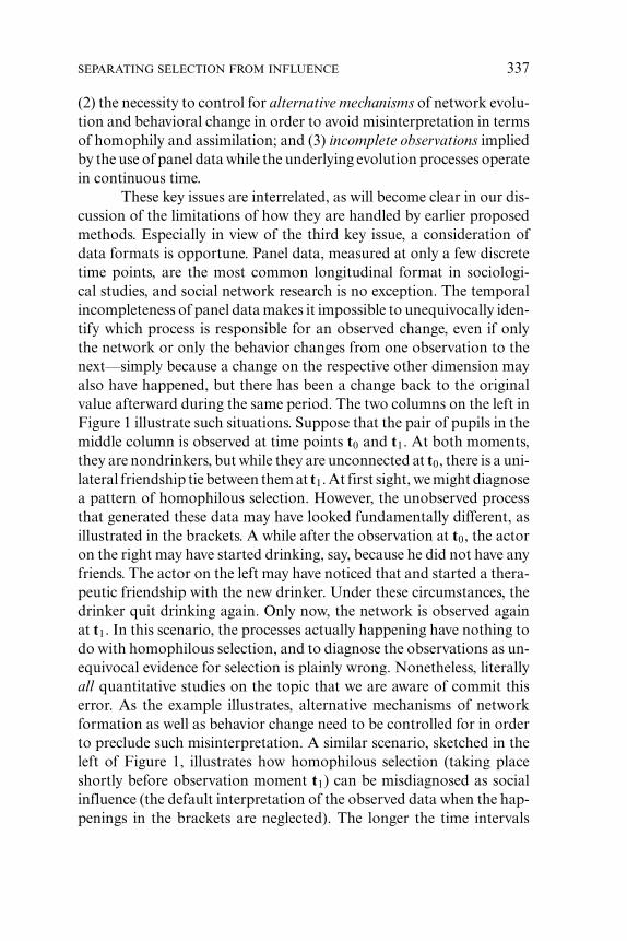
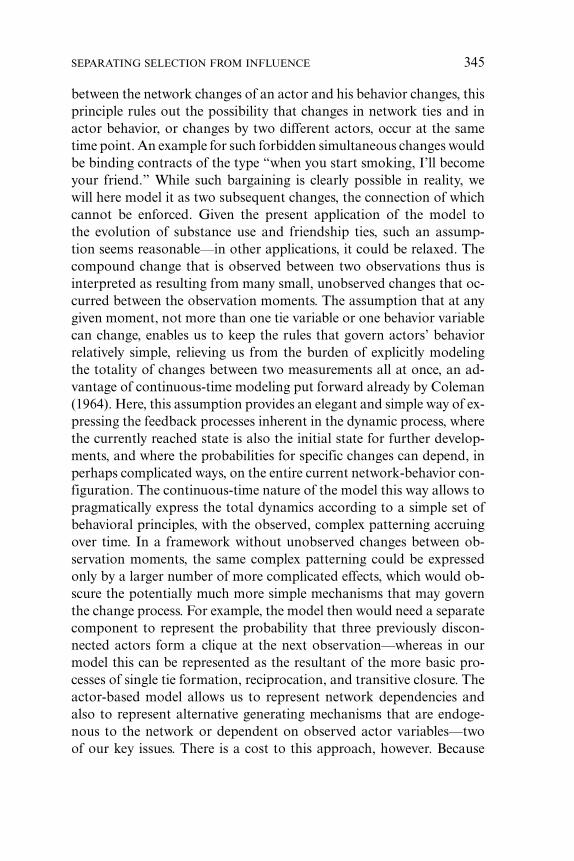
These key issues are interrelated, as will become clear in our dis-cussion of the limitations of how they are handled by earlier proposedmethods. Especially in view of the third key issue, a consideration ofdata formats is opportune. Panel data, measured at only a few discretetime points, are the most common longitudinal format in sociologi-cal studies, and social network research is no exception. The temporalincompleteness of panel data makes it impossible to unequivocally iden-tify which process is responsible for an observed change, even if onlythe network or only the behavior changes from one observation to thenext—simply because a change on the respective other dimension mayalso have happened, but there has been a change back to the originalvalue afterward during the same period. The two columns on the left inFigure 1 illustrate such situations. Suppose that the pair of pupils in themiddle column is observed at time points t0 and t1. At both moments,they are nondrinkers, but while they are unconnected at t0, there is a uni-lateral friendship tie between them at t1. At first sight, we might diagnosea pattern of homophilous selection. However, the unobserved processthat generated these data may have looked fundamentally different, asillustrated in the brackets. A while after the observation at t0, the actoron the right may have started drinking, say, because he did not have anyfriends. The actor on the left may have noticed that and started a thera-peutic friendship with the new drinker. Under these circumstances, thedrinker quit drinking again. Only now, the network is observed againat t1. In this scenario, the processes actually happening have nothing todo with homophilous selection, and to diagnose the observations as un-equivocal evidence for selection is plainly wrong. Nonetheless, literallyall quantitative studies on the topic that we are aware of commit thiserror. As the example illustrates, alternative mechanisms of networkformation as well as behavior change need to be controlled for in orderto preclude such misinterpretation. A similar scenario, sketched in theleft of Figure 1, illustrates how homophilous selection (taking placeshortly before observation moment t1) can be misdiagnosed as socialinfluence (the default interpretation of the observed data when the hap-penings in the brackets are neglected). The longer the time intervals
338 STEGLICH ET AL.
t0
t1
t0
t1
FIGURE 1. Illustrations for two of the three “key issues” mentioned in the text: incompleteobservation of changes (left and middle column) and alternative mechanisms (allcolumns).
are between observations, the higher the chances that such alternativetrajectories happen. Calculations based on our empirical study suggestthat on top of the observed changes, another 7–10% of changes remainunobserved because they cancel each other out before observation. Instudies on adolescent behavior, time intervals of one year are the rule,while scenarios as sketched in Figure 1 can reasonably be assumed totake place within a few months. The use of retrospective questions forassessing the particular relationship’s history (Kirke 2004) in principlecould remedy this predicament. However, retrospective social networkinformation is rare and prone to unreliability (Bernard et al. 1985), sothis remedy leads to other problems.
The problem of alternative generating mechanisms is not limitedto situations where the data are incompletely observed. In the columnon the right of Figure 1, the newly created tie could result from ho-mophilous selection (and indeed would be unequivocally diagnosed assuch by previous approaches in the literature). However, it could alsoresult from a purely structural mechanism known to play a strong rolein friendship formation—namely, triadic closure. Having a commonfriend at t0 may be the reason why at t1, a tie is established betweenthe two previously unrelated actors. The message is that even if we canassume that no unobserved changes have taken place, there still is in-terpretative leeway concerning the mechanisms responsible for a givenobserved change. Controlling for such mechanisms as far as possible isa criterion that previous research largely has failed to address.
Next to the temporal aspect of data collection, the cross-sectionaldesign is also important in distinguishing selection from influence
SEPARATING SELECTION FROM INFLUENCE 339
effects. There are two ideal types of social network studies: (1) ego-centered network studies, in which for a random sample of individuals(the egos), the network neighbors and their properties are assessed; and(2) complete network studies, in which for a given set of actors, all rela-tional links in this set are assessed, and the assumption is made that forthe research question being addressed, links outside of this set are lessconsequential and by approximation can be neglected. For the presentpurpose, an ego-centered network design is inadequate because evenin a panel study, such data do not provide information about other,potential relational partners that were not selected. This precludes ameaningful assessment of selection processes. For adequately measur-ing selection effects, a meaningful approximation of the set of potentialrelational partners must be made, whose individual properties must beknown irrespective of whether they actually become partners or not.In studies of complete networks, these data are available for all actorsin the network. Thus, a necessary condition for conducting a completenetwork study is that the delineation of the network gives a reasonableapproximation to the set of the actual and potential relational part-ners. However, this information comes at the price of dependence ofobservations, which rules out the application of the common statisticalprocedures, as these rely on independence of residuals. Depending onthe exact nature of the data-generating process, such procedures can bebiased toward conservative as well as liberal testing (Kenny and Judd1986; Bliese and Hanges 2004), and therefore lack reliability.
2.2. An Assessment of Previously Used Analytical Methods
There have been earlier attempts to separate selection effects from in-fluence effects, which we categorize in three main groups: (1) modelingfrequencies in a contingency table, (2) analyzing characteristics aggre-gated from the personal network, and (3) structural equation modeling.Here, we will briefly characterize these methods, in this order, and high-light the degree to which they meet the requirements on the three keyissues introduced.
In the contingency table approach, dyads of mutually chosenbest friends are typically cross-tabulated according to whether or notthe two pupils’ friendship remains stable between first and second mea-surement, and whether or not their behavior falls in the same, binary
340 STEGLICH ET AL.
category. Influence is typically assessed by studying the subsample ofrespondents who named the same best friend in both waves, while se-lection is assessed on the subsample of changing friendship ties. Forboth mechanisms, probabilities of change toward a behaviorally ho-mogeneous friendship are calculated, and based on these probabilities,predictions are generated for the whole sample of dyads. Significancetests for the two mechanisms are then derived by comparing these pre-dictions to the observed data, under the assumption of dyad indepen-dence. Prominent research that employs variants of this approach areKandel’s (1978) seminal study of marijuana use, educational aspira-tions, political orientation, and delinquency at New York State highschools, Billy and Udry’s (1985) study of adolescents’ sexual behavior,and Fisher and Bauman’s (1988) investigation of adolescents’ smok-ing and alcohol consumption. Our key issue of network dependence,here in the shape of inadequately assuming dyad independence, is usu-ally acknowledged as an acceptable weakness in this research. The twoother key issues, though, remain fully unaddressed. The use of incom-pletely observed data in particular puts a question mark over the results.Because the categorization of dyads in the contingency table is basedonly on the observed states at the beginning and at the end of theobservation period, the possibility of multiple explanatory trajectorieslinking these observations (as shown in Figure 1) is ruled out. Alterna-tive generating mechanisms, finally, can to some degree be controlledfor in this approach; see Fisher and Bauman (1988) for an example.However, triadic effects such as network closure or balance cannot becontrolled because of the restriction to dyads.
The studies we summarize as taking an aggregated personal net-work approach follow an explicit two-stage strategy. First, the networkdata are collapsed into summary statistics on the actor level, indicatingthe actor’s network position and properties of his personal network.Second, these reduced data are analyzed under independence assump-tions. Implicit in this approach is the assumption that all change isobserved and sufficiently reflected in the chosen statistics. The inde-pendence assumptions used in the second stage are clearly erroneous,which means that the studies cannot establish a firm statistical conclu-sion concerning processes of influence and selection. Next to leavingall our key issues unresolved, however, there are additional problemswith this approach. One is related to the arbitrariness in the choice
SEPARATING SELECTION FROM INFLUENCE 341
of the particular preprocessing algorithm. While Ennett and Bauman(1994), Pearson and Michell (2000), and Pearson and West (2003) makeuse of the negopy software (Richards 1995), which categorizes respon-dents into the four sociometric positions—group member, peripheral,liaison, and isolate—Cohen (1977) relies on a definition of sociomet-ric groups proposed by Coleman (1961), while Kirke (2004) relies onthe identification of weak components provided by the GRADAP soft-ware (Sprenger and Stokman 1995). The different options available atthis preprocessing stage are manifold, and their consequences are notwell-understood. More importantly, though, the reliance on the outputof such algorithms implies that network positions and neighborhoodproperties are used as if they were exogenously determined actor at-tributes. Further mutual interdependencies in the network structure, orthe specific identity of the peers, are not taken into account. A “groupmember” at one observation may still be identified as a “group member”at the subsequent observation, yet the groups referred to may consistof completely different peers. In such a situation, even the assumptionthat “the group” exerted social influence in the period in-between seemsdubious. Also, the selection of specific peers cannot be modeled in anactor-based analysis, and accordingly, the study of influence processesis not controlled for selection. As partial solution to the problem ofpeer identity, the actor-level statistics obtained in the first stage can becombined with an analysis on the dyad level under a contingency tableapproach; see Ennett and Bauman (1994) for an example.
The third type of studies that we distinguish here employ struc-tural equation models, specified as a cross-lagged panel or a latenttrajectory model, to assess selection and influence (Krohn et al. 1996;Iannotti et al. 1996; Simons-Morton and Chen 2005; De Vries et al.2006). This approach has been used for data collected using completenetwork as well as personal network designs. An advantage of this ap-proach over the other two is the relative ease with which selection andinfluence effects can be simultaneously assessed in the same analysis,controlling one for the occurrence of the other. The dependent vari-able for selection is defined here not at the dyadic level but by using avariable expressing peer behavior, which is an aggregate of the personalnetwork, usually defined as the average behavior of the current peers.In cross-lagged model specifications, there are paths from previous-wave respondent behavior to current-wave peer behavior, and from
342 STEGLICH ET AL.
previous-wave peer behavior to current-wave respondent behavior. Inthis setup, the estimated path coefficient from lagged peer behavior tocurrent respondent behavior is taken as a measure of peer influence,while the coefficient for the path from lagged respondent behavior tocurrent peer behavior is taken as an indicator for selection effects. Byestimating separate effects for old friends and new friends, the interpre-tation of path coefficients in terms of selection and influence is possi-ble, at least conceptually. However, the method still neglects the threekey issues of incomplete observations (estimated path coefficients di-rectly link the observed variables to each other), alternative generatingmechanisms (selection being modeled at an aggregate level precludesexpressing alternative mechanisms at the dyadic or triadic level), and—here especially important—the interdependence of observations. Whenthis approach is applied to complete network data, the individual re-spondent, whose behavior figures centrally in one observation, will alsoappear among the peers for other observations. This clearly violates in-dependence of observations, which is one of the crucial assumptions ofstructural equation modeling. While the use of ego-centered data wouldsolve this problem, it is not an option because it effectively precludes thestudy of selection processes, as outlined earlier. Mouw (2006) identifiesa number of other limitations of the cross-lagged panel specificationfor the case of ego-centered data, in particular that this specificationcontrols insufficiently for stable unobserved differences between respon-dents.
To summarize: the three analytical strategies covered here allfollow a two-stage procedure. In the first stage, the network data arecollapsed into individual-level variables (e.g., local density, centrality,indicators of group position, peer behavior) or dyad-level variables (be-havioral homogeneity), which in the second stage figure as variablesin more conventional analyses—as dependent variables for assessingselection effects, and as independent variables for assessing effects ofsocial influence. The shortcomings of such approaches are related tothe key issues introduced earlier. The stage of collapsing networksinto individual- or dyad-level data remains arbitrary and does not dofull justice to the structural aspect of evolving networks. In particu-lar, the use of such collapsed variables artificially freezes their valuesat the last preceding observation, which negates their endogenouslychanging nature and inhibits the study of potentially important feed-back mechanisms between network and behavior that are unobserved.
SEPARATING SELECTION FROM INFLUENCE 343
Alternative mechanisms that may be responsible for observed changesare generally difficult to control for in such models, especially whenthey express triadic or higher-order network effects such as closure orstructural balance. Finally, due to the problem of nonindependence ofactors and dyads, the first step of data reduction does not deliver datathat meet the requirements of the statistical procedures applied in thesecond-stage analyses.
3. A NEW APPROACH: MODELING THE COEVOLUTIONOF NETWORKS AND BEHAVIOR
A more principled statistical approach is possible by basing the dataanalysis on an explicit probability model for network-behavior coevo-lution that deals in a satisfactory way with the three key issues of net-work dependence, control for alternative mechanisms, and unobservedchanges in between observation moments. A computational model,which can be analyzed by means of computer simulations, is likely to bethe only satisfactory way to proceed. There is a rich tradition in compu-tational models for networks, and a smaller literature in which networkties as well as individual attributes change endogenously. Some exam-ples are Carley (1991), Macy et al. (2003), and Ehrhardt, Marsili, andVega-Redondo (2007). In part of this literature the changing attributesrefer to strategies played in games (e.g., Eguıluz et al. 2005). Researchin the physics literature on models of mutually dependent networksand attributes is reviewed by Gross and Blasius (2008). This literatureis mainly oriented toward deriving macrolevel properties of data setsimplied by models defined by relatively simple behavioral rules—but itis not very useful for purposes of statistical inference. Statistical mod-els for cross-sectional data with mutually dependent network ties wereproposed by Robins, Elliott, and Pattison (2001) and Robins, Pattison,and Elliott (2001), and are further discussed by Robins and Pattison(2005). For our purpose of longitudinal statistical analysis, we makeuse of the model proposed by Snijders and colleagues (2007), whichis an extension of earlier modeling work by Snijders (2001, 2005) fornetworks without coevolving behavioral dimensions. This model has atransparent definition as a stochastic process, and it is sufficiently flex-ible to incorporate a wide variety of alternative mechanisms. The pro-cess of network-behavioral coevolution is modeled here as an emergent
344 STEGLICH ET AL.
group-level result of interdependent behavioral changes occurring forsingle actors, and network changes occurring for pairs of actors. Onemajor characteristic of this model is its assumption that changes may oc-cur continuously between the observation moments. Models for paneldata that assume unobserved changes at arbitrary moments betweenpanel waves are particularly attractive for modeling feedback betweenmultiple variables. Such models are called continuous-time models,and they were proposed for discrete variables by Coleman (1964) anddiscussed for continuous variables, for example, by Arminger (1986)and Singer (1998). Holland and Leinhardt (1977) proposed to usecontinuous-time models specifically for network dynamics.
Handling the dynamic mutual dependence of the network tiesand the individual behavior requires a process model that specifies thesedependencies in a plausible way. The way to achieve this is based on thesecond major characteristic of this model, which is its actor-based archi-tecture. An explicit actor-based approach is in line with extant theoriesof individuals who act in the context of a social network. For exam-ple, for the study of friendship networks, taking the network actors asthe foci of modeling seems natural, as commonly invoked mechanismsof friendship formation (like homophily, reciprocity, or transitive clo-sure) are traditionally formulated and understood as forces operatingat the actor level, within the context of the network; the same holdsfor mechanisms of behavioral change (like social influence). Modelingthese changes in an actor-based framework implies that actors are as-sumed to “make” the change, by altering either their outgoing networkties or their behavior. The central model components will be the actors’behavioral rules determining these changes.
3.1. Action Rules and Occasions to Act
Some assumptions need to be made for the model to be tractable.Changes in network ties and behavior are assumed to happen in con-tinuous time, at stochastically determined moments. This allows us totackle the key issue of unobserved changes. We follow the principle,proposed by Holland and Leinhardt (1977) for network dynamics, todecompose the change process into its smallest steps. This is a way to ob-tain a relatively parsimonious model, and its implementation combinesin a natural way with the continuous time parameter. Distinguishing
SEPARATING SELECTION FROM INFLUENCE 345
between the network changes of an actor and his behavior changes, thisprinciple rules out the possibility that changes in network ties and inactor behavior, or changes by two different actors, occur at the sametime point. An example for such forbidden simultaneous changes wouldbe binding contracts of the type “when you start smoking, I’ll becomeyour friend.” While such bargaining is clearly possible in reality, wewill here model it as two subsequent changes, the connection of whichcannot be enforced. Given the present application of the model tothe evolution of substance use and friendship ties, such an assump-tion seems reasonable—in other applications, it could be relaxed. Thecompound change that is observed between two observations thus isinterpreted as resulting from many small, unobserved changes that oc-curred between the observation moments. The assumption that at anygiven moment, not more than one tie variable or one behavior variablecan change, enables us to keep the rules that govern actors’ behaviorrelatively simple, relieving us from the burden of explicitly modelingthe totality of changes between two measurements all at once, an ad-vantage of continuous-time modeling put forward already by Coleman(1964). Here, this assumption provides an elegant and simple way of ex-pressing the feedback processes inherent in the dynamic process, wherethe currently reached state is also the initial state for further develop-ments, and where the probabilities for specific changes can depend, inperhaps complicated ways, on the entire current network-behavior con-figuration. The continuous-time nature of the model this way allows topragmatically express the total dynamics according to a simple set ofbehavioral principles, with the observed, complex patterning accruingover time. In a framework without unobserved changes between ob-servation moments, the same complex patterning could be expressedonly by a larger number of more complicated effects, which would ob-scure the potentially much more simple mechanisms that may governthe change process. For example, the model then would need a separatecomponent to represent the probability that three previously discon-nected actors form a clique at the next observation—whereas in ourmodel this can be represented as the resultant of the more basic pro-cesses of single tie formation, reciprocation, and transitive closure. Theactor-based model allows us to represent network dependencies andalso to represent alternative generating mechanisms that are endoge-nous to the network or dependent on observed actor variables—twoof our key issues. There is a cost to this approach, however. Because
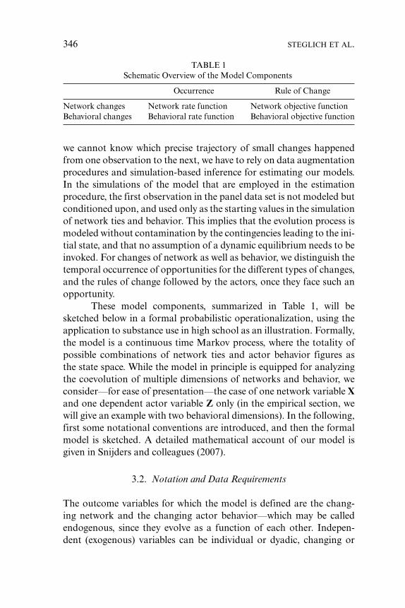
346 STEGLICH ET AL.
TABLE 1Schematic Overview of the Model Components
Occurrence Rule of Change
Network changes Network rate function Network objective functionBehavioral changes Behavioral rate function Behavioral objective function
we cannot know which precise trajectory of small changes happenedfrom one observation to the next, we have to rely on data augmentationprocedures and simulation-based inference for estimating our models.In the simulations of the model that are employed in the estimationprocedure, the first observation in the panel data set is not modeled butconditioned upon, and used only as the starting values in the simulationof network ties and behavior. This implies that the evolution process ismodeled without contamination by the contingencies leading to the ini-tial state, and that no assumption of a dynamic equilibrium needs to beinvoked. For changes of network as well as behavior, we distinguish thetemporal occurrence of opportunities for the different types of changes,and the rules of change followed by the actors, once they face such anopportunity.
These model components, summarized in Table 1, will besketched below in a formal probabilistic operationalization, using theapplication to substance use in high school as an illustration. Formally,the model is a continuous time Markov process, where the totality ofpossible combinations of network ties and actor behavior figures asthe state space. While the model in principle is equipped for analyzingthe coevolution of multiple dimensions of networks and behavior, weconsider—for ease of presentation—the case of one network variable Xand one dependent actor variable Z only (in the empirical section, wewill give an example with two behavioral dimensions). In the following,first some notational conventions are introduced, and then the formalmodel is sketched. A detailed mathematical account of our model isgiven in Snijders and colleagues (2007).
3.2. Notation and Data Requirements
The outcome variables for which the model is defined are the chang-ing network and the changing actor behavior—which may be calledendogenous, since they evolve as a function of each other. Indepen-dent (exogenous) variables can be individual or dyadic, changing or
SEPARATING SELECTION FROM INFLUENCE 347
unchanging. We make use of the following notation. The network isassumed to be based in a group of N actors—for example, a cohort ofpupils at the same school, or business firms active in the same periodin the same industry. The network is denoted by x, where xij(t) standsfor the value of the directed relationship between actors i and j at timepoint t. Examples for such relational variables are friendship betweenthe pupils of a year group, advice among employees in an organiza-tion, or share ownership between business firms. We assume that x isdichotomous—that is, xij = 1 stands for presence of a tie and xij = 0 forabsence. Next, z denotes the behavioral variable, with zi(t) standing forthe score of actor i at time point t. Examples here are the smoking be-havior of pupils, the performance of employees, or the activity in a givenmarket segment of a business firm. We assume that behavioral dimen-sions are measured on a discrete, ordinal scale represented by integervalues (e.g., dichotomous scales). Finally, v and w denote actor-leveland dyad-level exogenous covariates, respectively (for ease of presenta-tion here assumed to be constant over time), with v(k)
i standing for thescore of actor i on actor covariate k, and w(k)
ij standing for the dyadiccovariate k measured for the pair (ij). Typical actor covariates are sex,age, or education of a pupil or an employee, or number of employees of abusiness firm. Examples for dyadic covariates could be a classmate rela-tion between pupils in a year group, an organizational hierarchy betweenemployees, or the geographical distance of business firms.
We consider the case of network-behavior panel data, where thenetwork and behavioral data are collected for a finite set of time pointsonly (say, t1 < t2 < · · · < tM), with at least M = 2 waves. In the fol-lowing section, the data are indicated by lowercase letters (networksx(t1) , . . . , x(tM), behavior z(t1) , . . . , z(tM), etc.), while the stochasticmodel components (of which these data are assumed to be realizations)are indicated by uppercase letters (network model X(t) and behavioralmodel Z(t)). The formal model is obtained by spelling out the submod-els indicated in Table 1 and integrating them into the overall model.Although the objective functions are the most important model compo-nents, for ease of presentation we first explain the model for occurrenceof changes.
3.3. Modeling Opportunities for Change
The assumption was already mentioned that at any single moment,only one tie variable or one behavioral variable may change. More
348 STEGLICH ET AL.
specifically, it is assumed that at stochastically determined moments,one actor gets the opportunity to change one of his or her outgoingtie variables, or to change his or her behavior. Such opportunities forchange are called micro steps. It is also allowed that the actor doesnot make a change but leaves things as they are. The frequency bywhich actors have the opportunity to make a change is modeled byrate functions, one for each type of change. The main reason for havingseparate rate functions for the behavioral and the network changes isthat practically always, one type of decision will indeed be made morefrequently than the other. In information flow networks, for example,we can expect that the actors’ individual properties (here: knowledgestates) change more quickly than their network ties. In group formationprocesses, where the behavioral dimensions may represent attitudes, theopposite may be true. In the application to substance use and friendshipat high school, we would expect more frequent changes in the networkthan in substance use, caused by (1) the addictive nature of substanceuse and (2) the students’ social orientation phase in adolescence.
The first observations of network ties x(t1) and behavior z(t1)serve as starting values of the evolution process — that is, they are notmodeled themselves but conditioned upon, and only the subsequentchanges of network ties and behavior are modeled. In order to obtaina Markov process, waiting times between micro steps must have expo-nential distributions, as this is the only distribution with the lack ofmemory property (Norris 1997). For each actor i and for network andbehavioral changes alike, we model the waiting time until actor i takesa micro step by exponentially distributed variables Ti
net and Tibeh with
parameters λinet > 0 and λi
beh > 0, i.e., the waiting times are distributedsuch that Pr(T > t) = exp(−λt) for all t > 0. The parameters of thesedistributions indicate the rate (or speed) at which the respective changeis likely to occur; the expected waiting time is 1/λ. Since actual waitingtimes between changes are not observed, more complicated modelingis unwarranted. It is further assumed that all waiting times are indepen-dent, given the current state of network and behavior. Properties of theexponential distribution imply that, starting from any given moment intime (e.g., the moment of the preceding micro step), the waiting timeuntil occurrence of the next micro step of either kind by any actor isexponentially distributed with parameter
λtotal =∑
i
(λnet
i + λbehi
). (1)
SEPARATING SELECTION FROM INFLUENCE 349
The probability that this is a network micro step taken by aparticular actor i is given by
λneti
/λtotal, (2)
and the probability that this is a behavior micro step taken by a partic-ular actor i is given by
λbehi
/λtotal. (3)
There may be heterogeneity in the activity of actors — some ac-tors may change their network ties, or their behavior, more quickly thanothers. Such activity differences may be caused by individual properties(e.g., by sex differences) or by an existing network structure (e.g., by thenumber of ties an actor already has). We can incorporate such activitydifferences between actors by letting the parameters λ that govern therate functions depend on actor attributes and network positions, as inSnijders (2001, 2005). In this paper, however, we limit the discussionto model specifications where both types of rate functions are constantacross actors, and depend only on the periods between panel waves.Accordingly, from here onward, the lower index m of a rate λtype
m willdenote a time period, 1 ≤ m ≤ M, not an individual anymore.
3.4. Modeling Mechanisms of Change
What happens in a micro step is modeled as the outcome of changesmade by the actors. Micro steps can be of two kinds, correspondingto network changes or behavioral changes. For network changes, themicro step consists of the change of one tie variable by a given actor.Say x is the current network and actor i has the opportunity to makea network change. The next network state x′ then must be either equalto x (i.e., keep the current situation) or deviate from x in exactly oneelement in row i (i.e., change the tie variable linking actor i to oneother actor). From these N possible outcomes, it is assumed that ichooses that value x′ for which fnet
i (x, x′, z) + εneti (x, x′, z) is maximal.
Here z is the current vector of behavior scores, fnet is a deterministicobjective function that can be interpreted loosely as a measure of theactor’s satisfaction with the result of the network decision (“what the
350 STEGLICH ET AL.
actor strives for when changing network ties”), and εnet is a randomdisturbance term representing unexplained change. By making someconvenient standard assumptions about the distribution of the randomcomponent (McFadden 1974; Pudney 1989), the choice probabilitiescan be expressed in multinomial logit shape,
exp(fneti (x′, z)
)/∑x′′
exp(fneti (x′′, z)
), (4)
where the sum in the denominator extends over all possible next networkstates x′′. This model for tie probabilities was used also by Snijders(2001) and Powell and colleagues (2005).
In a behavioral micro step, following again the parsimoniousmodeling principle that changes occur in the smallest possible steps, itis assumed that a given actor either increments or decrements his score onthe behavioral variable by one unit, provided that this change does notstep outside the range of this variable; it is also assumed that the scoreis not changed. The modeling is completely analogous to that of thenetwork micro steps. If z is the current vector of behavior scores for allactors, and i is the actor allowed to change his behavior, let z′ denote thevector resulting from an allowed micro step. It is allowed that i choosesthat value z′ for which fbeh
i (x, z, z′) + εbehi (x, z, z′) is maximal, where
now fbeh is a different deterministic objective function that again can beinterpreted as the actor’s satisfaction with the result of the behavioraldecision, and εbeh again is a random disturbance term representingunexplained change. By making appropriate assumptions about thedistribution of the random component, choice probabilities can also beexpressed in multinomial logit shape,
exp(fbehi (x, z′)
)/∑z′′
exp(fbehi (x, z′′)
), (5)
where now the sum in the denominator extends over all possible nextbehavior states z′′. This type of model, for changes in an ordinal variablenot combined with network ties, was used also by Chan and Munoz-Hernandez (2003).
It may be noted here that the model formulation in terms ofchoice models does in no way imply that we assume actors to befully strategically rational, let alone that estimated parameters for the
SEPARATING SELECTION FROM INFLUENCE 351
objective functions express respondents’ actual preferences. Becausethe states’ evaluations in terms of the objective function are being com-pared immediately after a contemplated micro step, the actors’ behaviorlacks the strategic element of considering reactions from other actors.The model therefore can best be viewed as an instantiation of myopicrationality, following Luce’s (1959) rationality axioms.
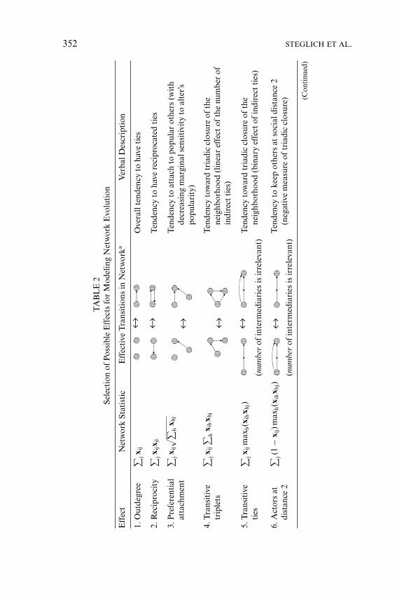
The focus of modeling is on the deterministic parts, defined by theobjective functions f. A high degree of flexibility is achieved by modelingthese as linear combinations of effects that express the dependence ofnetwork and behavior on each other as well as on externally givenvariables. The term exogenous will be used for effects depending onsuch external variables, while endogenous effects depend on the currentvalues of the dependent variables (networks and behavior). For networkchanges, the objective function has the general shape fnet
i (x, x′, z) =∑h βnet
h sneth (i, x, x′, z), where statistics snet
h stand for the effects, weightedby parameters βnet
h whose size is determined by fitting the model to thedata. Analogously, the objective function for behavioral changes hasthe form fbeh
i (x, z, z′) = ∑h βbeh
h sbehh (i, x, z, z′). The statistics, or effects,
must be defined on substantive grounds based on theory and fieldknowledge. They are arbitrary from the point of view of mathematicalmodeling, although in practice it is an advantage that they are nottoo complicated computationally. The most important network andbehavior effects depend only on the new states x′ and z′, not on theprevious states x and z, and their weights β can be interpreted as thedegree to which the actors have a tendency to change into a directionwhere the network-behavioral state has high values for these effects. Aselection of possible endogenous network effects snet
h is given in Table 2,while a similar selection of effects sbeh
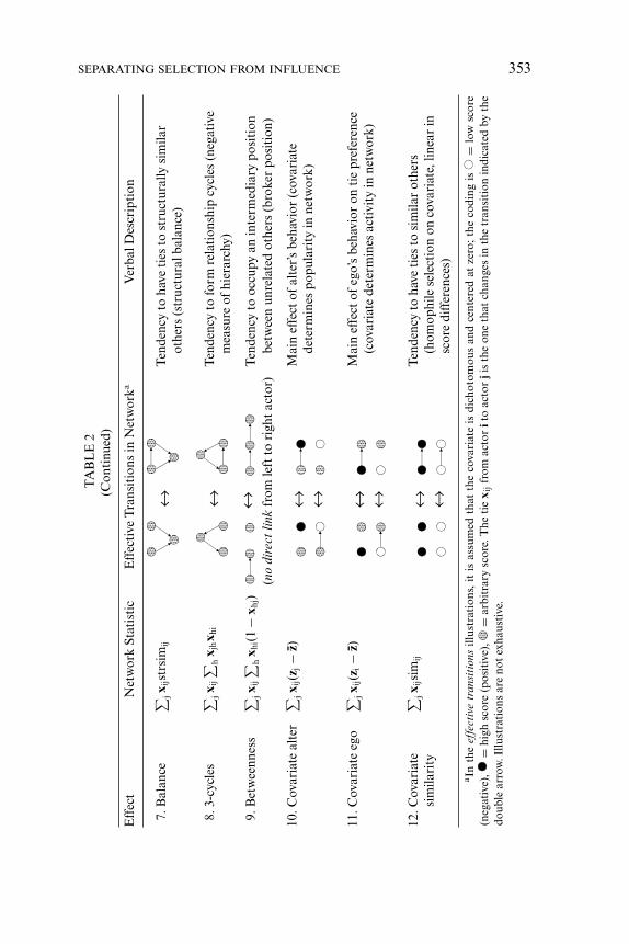
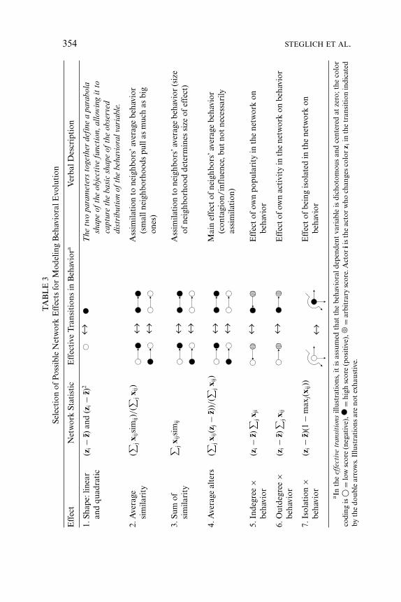
h for behavioral changes is givenin Table 3. These components are based on indicators of structuralpositions in networks that are of fundamental importance in socialnetwork analysis (Wasserman and Faust 1994). The second columnof these tables contains the formulas of the statistics that express therespective effects.
In these tables, similarity of the behavioral scores of two ac-tors i and j is defined as simij = 1 − |zi − zj|/rangeZ, where the rangeof behavioral scores is defined as the maximum minus the minimum ofobserved values. By this definition, similarity is standardized to the unitinterval, sim = 0 indicating maximally dissimilar scores and sim = 1indicating identical (i.e., maximally similar) scores. For the calculations
352 STEGLICH ET AL.
TA
BL
E2
Sele
ctio
nof
Poss
ible
Eff
ects
for
Mod
elin
gN
etw
ork
Evo
luti
on
Eff
ect
Net
wor
kSt
atis
tic
Eff
ecti
veT
rans
itio
nsin
Net
wor
kaV
erba
lDes
crip
tion
1.O
utde
gree
∑ jx i
jO
vera
llte
nden
cyto
have
ties
2.R
ecip
roci
ty∑ j
x ijx
jiT
ende
ncy
toha
vere
cipr
ocat
edti
es
3.P
refe
rent
ial
atta
chm
ent
∑ jx i
j√ ∑h
x hj
Ten
denc
yto
atta
chto
popu
lar
othe
rs(w
ith
decr
easi
ngm
argi
nals
ensi
tivi
tyto
alte
r’s
popu
lari
ty)
4.T
rans
itiv
etr
iple
ts
∑ jx i
j∑ h
x ihx h
jT
ende
ncy
tow
ard
tria
dic
clos
ure
ofth
ene
ighb
orho
od(l
inea
ref
fect
ofth
enu
mbe
rof
indi
rect
ties
)
5.T
rans
itiv
eti
es
∑ jx i
jm
axh(x
ihx h
j)T
ende
ncy
tow
ard
tria
dic
clos
ure
ofth
ene
ighb
orho
od(b
inar
yef
fect
ofin
dire
ctti
es)
(num
ber
ofin
term
edia
ries
isir
rele
vant
)
6.A
ctor
sat
dist
ance
2
∑ j(1
−x i
j)m
axh(x
ihx h
j)T
ende
ncy
toke
epot
hers
atso
cial
dist
ance
2(n
egat
ive
mea
sure
oftr
iadi
ccl
osur
e)(n
umbe
rof
inte
rmed
iari
esis
irre
leva
nt)
(Con
tinu
ed)
SEPARATING SELECTION FROM INFLUENCE 353T
AB
LE
2(C
onti
nued
)
Eff
ect
Net
wor
kSt
atis
tic
Eff
ecti
veT
rans
itio
nsin
Net
wor
kaV
erba
lDes
crip
tion
7.B
alan
ce∑ j
x ijs
trsi
mij
Ten
denc
yto
have
ties
tost
ruct
ural
lysi
mila
rot
hers
(str
uctu
ralb
alan
ce)
8.3-
cycl
es∑ j
x ij∑ h
x jhx h
iT
ende
ncy
tofo
rmre
lati
onsh
ipcy
cles
(neg
ativ
em
easu
reof
hier
arch
y)
9.B
etw
eenn
ess
∑ jx i
j∑ h
x hi(1
−x h
j)T
ende
ncy
tooc
cupy
anin
term
edia
rypo
siti
on(n
odi
rect
link
from
left
tori
ght
acto
r)be
twee
nun
rela
ted
othe
rs(b
roke
rpo
siti
on)
10.C
ovar
iate
alte
r∑ j
x ij(z
j−
z)M
ain
effe
ctof
alte
r’s
beha
vior
(cov
aria
tede
term
ines
popu
lari
tyin
netw
ork)
11.C
ovar
iate
ego
∑ jx i
j(zi−
z)M
ain
effe
ctof
ego’
sbe
havi
oron
tie
pref
eren
ce(c
ovar
iate
dete
rmin
esac
tivi
tyin
netw
ork)
12.C
ovar
iate
sim
ilari
ty
∑ jx i
jsim
ijT
ende
ncy
toha
veti
esto
sim
ilar
othe
rs(h
omop
hile
sele
ctio
non
cova
riat
e,lin
ear
insc
ore
diff
eren
ces)
aIn
the
effe
ctiv
etr
ansi
tion
sill
ustr
atio
ns,
itis
assu
med
that
the
cova
riat
eis
dich
otom
ous
and
cent
ered
atze
ro;
the
codi
ngis
=lo
wsc
ore
(neg
ativ
e),
=hi
ghsc
ore
(pos
itiv
e),
=ar
bitr
ary
scor
e.T
heti
ex
ijfr
omac
tor
ito
acto
rji
sth
eon
eth
atch
ange
sin
the
tran
siti
onin
dica
ted
byth
edo
uble
arro
w.I
llust
rati
ons
are
not
exha
usti
ve.
354 STEGLICH ET AL.T
AB
LE
3Se
lect
ion
ofPo
ssib
leN
etw
ork
Eff
ects
for
Mod
elin
gB
ehav
iora
lEvo
luti
on
Eff
ect
Net
wor
kSt
atis
tic
Eff
ecti
veT
rans
itio
nsin
Beh
avio
raV
erba
lDes
crip
tion
1.Sh
ape:
linea
ran
dqu
adra
tic
(zi−
z)an
d(z
i−
z)2
The
two
para
met
ers
toge
ther
defi
nea
para
bola
shap
eof
the
obje
ctiv
efu
ncti
on,a
llow
ing
itto
capt
ure
the
basi
csh
ape
ofth
eob
serv
eddi
stri
buti
onof
the
beha
vior
alva
riab
le.
2.A
vera
gesi
mila
rity
(∑ jx i
jsim
ij)/
(∑ jx i
j)A
ssim
ilati
onto
neig
hbor
s’av
erag
ebe
havi
or(s
mal
lnei
ghbo
rhoo
dspu
llas
muc
has
big
ones
)
3.Su
mof
sim
ilari
ty
∑ jx i
jsim
ijA
ssim
ilati
onto
neig
hbor
s’av
erag
ebe
havi
or(s
ize
ofne
ighb
orho
odde
term
ines
size
ofef
fect
)
4.A
vera
geal
ters
(∑ jx i
j(zj−
z))/
(∑ jx i
j)M
ain
effe
ctof
neig
hbor
s’av
erag
ebe
havi
or(c
onta
gion
/inf
luen
ce,b
utno
tne
cess
arily
assi
mila
tion
)
5.In
degr
ee×
beha
vior
(zi−
z)∑ j
x ji
Eff
ect
ofow
npo
pula
rity
inth
ene
twor
kon
beha
vior
6.O
utde
gree
×be
havi
or(z
i−
z)∑ j
x ij
Eff
ecto
fow
nac
tivi
tyin
the
netw
ork
onbe
havi
or
7.Is
olat
ion
×be
havi
or(z
i−
z)(1
−m
axj(x
ij))
Eff
ect
ofbe
ing
isol
ated
inth
ene
twor
kon
beha
vior
aIn
the
effe
ctiv
etr
ansi
tion
sill
ustr
atio
ns,i
tis
assu
med
that
the
beha
vior
alde
pend
ent
vari
able
isdi
chot
omou
san
dce
nter
edat
zero
;the
colo
rco
ding
is�
=lo
wsc
ore
(neg
ativ
e),
=hi
ghsc
ore
(pos
itiv
e),
=ar
bitr
ary
scor
e.A
ctor
iis
the
acto
rw
hoch
ange
sco
lor
z iin
the
tran
siti
onin
dica
ted
byth
edo
uble
arro
ws.
Illu
stra
tion
sar
eno
tex
haus
tive
.
SEPARATING SELECTION FROM INFLUENCE 355
of the statistics in the tables, similarity is further centered around theempirical average over all measurement points. Such centering reducesestimation difficulties caused by collinearity. Therefore, the covariatesand behavioral variables are also centered (which, in this case, can beseen back in the formulas). The balance effect for network evolution(Davis 1963; Mizruchi 1993) contains a measure of structural similaritystrsimij = ∑
h (b − |xih − xjh|) that is analogous to similarity, where b isa parameter used for standardization. In network terms, this may beregarded as a measure for structural equivalence regarding outgoingties (Lorrain and White 1971). The tables can naturally give only aglimpse of the complexity and richness of modeling that becomes pos-sible within the proposed framework and may be elaborated in futureresearch.
3.5. Integration of Model Components and Model Estimation
The total model specification for network-behavioral coevolution con-sists of the first wave observations x(t1) and z(t1) as the initial state of thestochastic process, the rate functions defining the rates of occurrence ofnetwork or behavioral micro steps by specific actors as sketched above,and the choice probabilities for each possible micro step. As a whole, themodel belongs to the class of continuous time Markov chains (e.g., Norris1997). The description given above allows us to construct a computersimulation of this process and also to specify the so-called intensitymatrix which is the mathematical characterization of the Markov chainprocess (cf. see Snijders et al. 2007).
For given sets of parameter values, the evolution model can beimplemented as a stochastic simulation algorithm that can be usedto generate network and behavioral data according to the postulateddynamic process. Since the model is a Markov chain, the simulationalgorithm is defined by giving the step of a single change in the process.We start out at some network-behavior configuration (x(t), z(t)). First,a waiting time is drawn from the exponential distribution with param-eter (1), and the time parameter t is incremented by this waiting time.The process stops when time exceeds the end time of the period. If itcontinues, using probabilities (2) and (3), it is determined whether thenext event is a network change or a behavior change, and who is theactor making the change. The change to be made is chosen according
356 STEGLICH ET AL.
to probabilities (4) or (5), respectively. The process repeats itself untilthe end of the period is reached. At that point, the resulting simulatednetwork-behavior configuration can be evaluated.
The model is too complex to allow for closed-form calculations ofprobabilities, expected values, etc., which is why direct ways of parame-ter estimation such as maximum likelihood are not easily implemented.However, the simulation algorithm can be employed to determine pa-rameter estimates as those values under which simulated and observeddata resemble each other most closely. This idea is instantiated in themethod of moments estimation routine, which is used in the empiricalsection of this paper. To define it, each model parameter θ. must bematched with a statistic S. that can be evaluated on a given data set (beit simulated or observed), and which defines an estimation equation forthis parameter by demanding that the expected value over simulationsis equal to the observed value of the statistic. The vector of parameterestimates is obtained as the joint solution to the corresponding systemof equations. For network-behavior coevolution models, Snijders andcolleagues (2007) proposed the following four types of statistics for thefour types of model parameters according to Table 1:
Network rate, period m θ. = λnetm S. =
∑ij
|Xij(tm+1) − xij(tm)|
Behavior rate, period m θ. = λbehm S. =
∑i
|Zi(tm+1) − zi(tm)|
Network objective θ. = βneth S. =
∑m
∑i
sneth (i, X(tm+1), z(tm))
function effects
Behavior objective θ. = βbehh S. =
∑m
∑i
sbehh (i, x(tm), Z(tm+1))
function effects
The expected value over simulations of each of these estima-tion statistics S. can be understood as a function of the vector θ of allmodel parameters, and it is typically monotone increasing in its “own”parameter. Under mild regularity conditions (nondegeneracy of the ma-trix D of partial derivatives of statistics S by parameters θ), parameterscan be uniquely identified. Notice the “cross-lagged” combination ofsimulated data at the end of an observation period with observed data
SEPARATING SELECTION FROM INFLUENCE 357
at the beginning of the period, on which the estimation statistics for ob-jective function parameters are based. Here it is ensured that selectionand influence processes that result in the same cross-sectional patternscan be empirically distinguished, provided that the lagged statistic isreasonably stable over time.
The iterative procedure by which parameter estimates and stan-dard errors are obtained is described in detail by Snijders (2001) and bySnijders and colleagues (2007), and it can be sketched as follows. Theiterations start at a parameter value θ0, and at step k they have reachedthe current trial parameter value θk. The process is then simulated ac-cording to this parameter value, yielding simulated statistics Ssim
k . Afterthis simulation, the parameter is updated according to the equationθk+1 = θk − ak+1D−1
0 (Ssimk − Sobs), where D0 is an approximation of the
matrix of partial derivatives of statistics S by parameters θ evaluated atθ0, where Sobs is the observed vector of estimation statistics, and whereak is a sequence of numbers that approach zero at rate k−c; c is chosenfrom the interval 0.5 < c < 1 so as to obtain good convergence prop-erties. The final estimate is defined as a tail average of the trial values,θ = 1
R
∑Rr=1 θ r0+r, where the initial number of trials r0 is long enough
for a suitable burn-in period, and R is large enough to obtain a stableestimate. Standard errors of the estimate θ are calculated as the squareroots of the diagonal elements of the approximate covariance matrixof the estimator function θ , evaluated at the estimate, as given by theequation covθ (θ ) = D−1
θ�θ (S)Dθ . Here �θ (S) stands for the matrix of
simulated covariance of the vector of estimation statistics, evaluated atthe estimate, and D is again the (approximate) derivative matrix, nowevaluated at the estimate.
Parameter estimation for this type of model has been broadlycategorized as “third generation problems” in applied statistics(Gourieroux and Monfort 1996) and it is computationally intensive.Depending on the data set and the model, it is possible—but rare—thatthe algorithm does not converge in a satisfactory way. This happensfor models that are complicated in the sense that there are too manyparameters relative to the variation in the data, or when effects arehighly correlated in the data. Nonconvergence may also be an indicatorof model misspecification. In the large majority of cases, however, withdata sets ranging between 30 and a few hundred actors, and when theamount of change between successive waves is not too large while the
358 STEGLICH ET AL.
amount of change between the first and last waves is large enough, ourexperience is that convergence results are good.
3.6. Interpretation of Model Parameters
As a consequence of the actor-based nature of modeling and the de-composition of observed transitions from one observation to the nextas a sequence of unobserved small changes, special attention needs tobe paid to the interpretation of the estimated model parameters. Theparameters of the rate functions can be related directly to the speedof the evolution process—keeping in mind that they reflect frequenciesof opportunities for change, not frequencies of actual change, and thatactors who are near the optimum of their objective functions will havea smaller probability of utilizing their opportunity for change. The pa-rameters of the objective functions, however, relate in a more indirectway to the observed global dynamics of network and behavior. Froma perspective of agency, these functions can be regarded as satisfactionmeasures of the actors with their local network-behavioral neighbor-hood. At a less construing level, they can be thought of descriptively, asa summary expression of the behavioral rules that are likely to be fol-lowed by the actors, given the observed data. These objective functions,together with the current network-behavior configuration, imply spe-cific global dynamics as emergent property of the individual changes,in which network actors are mutually constraining each other and mu-tually offering opportunities to each other in a feedback process. Inorder to understand how the estimated parameters of the objectivefunctions relate to the global dynamics observed, the Markov prop-erty of the process model needs to be invoked. This property impliesthat corresponding to the parameters there is a stationary (equilib-rium) distribution of probabilities over the state space of all possiblenetwork-behavior configurations. Because the data configuration ob-served in the first wave of the panel will often not be in the center ofthis equilibrium distribution, the model defines a nonstationary processof network-behavioral dynamics, starting at the first observation andthen “drifting” toward those states that have a relatively high probabil-ity under the equilibrium distribution; for the mathematical principles,see Norris (1997), for example. The dynamics as well as the station-ary distribution of all but the simplest cases of these models are too
SEPARATING SELECTION FROM INFLUENCE 359
complex for analytic calculations, but they can be investigated by com-puter simulation.
For the “immediate interpretation” of the parameters of theobjective functions, it can be useful to consider the odds of some-what idealized micro steps (this is similar to the interpretation of pa-rameters obtained by logistic regression). Suppose an actor i is in asituation to make a network micro step, and suppose two alterna-tive courses of action result in networks xA and xB. From the lin-ear shape of the objective function and the multinomial logit prob-abilities for micro steps, the odds for these outcomes can be derivedas Pr(xA)/Pr(xB) = exp(
∑h βnet
h [sneth (xA) − snet
h (xB)]), in simplified no-tation. As can be seen from this formula, the odds depend on thedegree to which the two networks differ on the actor-specific statis-tics snet
h (see again Table 2), these differences being weighted by themodel parameters. Likewise, if the actor is in a situation to make abehavioral micro step and is considering two alternative courses of ac-tion resulting in behavioral vectors zA and zB, the odds are given byPr(zA)/Pr(zB) = exp(
∑h βbeh
h [sbehh (zA) − sbeh
h (zB)]).By way of example, let us assume that in a simple model
specification, the function fneti (x, x′, z) = −2.0
∑j x′
ij + 2.5∑
j x′ijxji +
1.0∑
j x′ijsimij was estimated as a typical network objective function,
while the behavioral objective function was estimated as fbehi (x, z, z′) =
−1.0(z′i − z) − 0.5(z′
i − z)2 + 2.5(∑
j xijsim′ij)/(
∑j xij), also quite typi-
cal. The primes indicate those elements in the formulas the values ofwhich are under the control of actor i and may be changed in a microstep that is governed by the objective function in which they occur.The network objective function contains three effects: (1) the outdegreeeffect (with parameter estimate βnet
out = −2.0), (2) the reciprocity effect(with parameter estimate βnet
rec = 2.5), and (3) the similarity effect (withparameter estimate βnet
sim = 1.0). In the behavioral objective function,the model contains three more effects: (1) an effect with two parametersdetermining the basic shape of the distribution of the variable, (2) onelinear (with estimate βbeh
lin = −1.0) and one quadratic (with estimateβbeh
quad = −0.5) effect, and (3) an effect of average similarity to neighbors(with parameter estimate βbeh
av.sim = 2.5). We now address the questionof how these parameter values can be interpreted, starting with thenetwork objective function.
The parameter attached to the outdegree effect in the networkobjective function has a negative sign, which indicates that observed
360 STEGLICH ET AL.
network densities are low. If the objective function were constant zero(i.e., if the outdegree parameter and all other parameters are zero), thenetwork micro steps would, according to the odds formula above, leadin the long run to a network of density 0.5. In other words, 50% of allpossible ties would be present in such equilibrium networks. Empiricaldensities in most social networks are much lower than 0.5, and therefore,the outdegree parameter (which models the general tendency of theactors to send out ties in the network, hence indirectly also the densityof the network) is typically strongly negative. If we for the momentdisregard the other parameters, the value of –2.0 for the outdegreeparameter means that upon an opportunity for change, the odds forany tie to be present versus absent are exp(−2.0) ≈ 0.135.
The reciprocity parameter accounts for the observed degree ofreciprocity in the networks. If the objective function consisted only ofthe outdegree effect and if the reciprocity parameter was zero, the microsteps would in the long run lead to a network in which the incomingand outgoing ties are independent. In such a situation, reciprocatedties in sparse networks would be very unlikely. However, many sparsesocial relations, such as friendship, exhibit a relatively high degree ofreciprocation. For modeling these relations, the reciprocity parameter(which models the general tendency of the actors to reciprocate incom-ing ties by sending back an outgoing tie) is typically strongly positive.The objective function value associated with a reciprocated tie is calcu-lated by adding to the outdegree parameter value (for having the tie) thereciprocity parameter value (for the additional property of reciprocity),which amounts to a net value of –2.0 + 2.5 = 0.5 for a reciprocated tie.Making use of the odds formula above, the odds of reciprocating anincoming tie versus not reciprocating it are exp(0.5) ≈ 1.65.
The positive similarity effect in our example indicates that actorstend to have ties to similar others rather than to dissimilar ones; theodds are ceteris paribus 2.72 for a tie to a maximally similar actor versusa maximally dissimilar actor. By including this effect, homophilousselection based on the behavioral variable can be modeled.
So far, the odds calculations referred only to the existence ofa tie versus nonexistence, but they could also be more complex. Forinstance, the odds of reciprocating an incoming tie to a dissimilar ac-tor versus creating a unilateral, unreciprocated tie to a similar one areexp(0.5 + 2.0 − 1.0) ≈ 4.48. As in logistic regression, the calculation ofodds becomes more complex as the model has more components and
SEPARATING SELECTION FROM INFLUENCE 361
as one is willing to distinguish more variable configurations. We mustkeep in mind that all odds calculations are model-derived and refer toartificial comparisons, since they hold only under a ceteris paribus as-sumption. Accordingly, for determining their validity, they need to beconsidered in light of how the actual data look—here reflected in theempirical values of the statistics s—and whether a specific odds calcula-tion derived from an estimated model refers to situations that frequentlyoccur in the data (then validity is less problematic) or not (then calcu-lation of the odds in question may be an unwarranted extrapolation).In general, the more effects one is willing to consider (and estimate) si-multaneously, the less analytically tractable the model-explained globaldynamics get, and the more one needs to consult simulations for learn-ing about what an estimated model means in terms of global networkproperties.
In the example above, we now consider the behavior objectivefunction, which contains three more parameters. The first two arethe linear and quadratic shape parameters, which model the shapeof the long-term distribution of the behavior variable. Let us assumethat the possible scores on the behavioral variable range from 1 to 5and that the observed average over all time points is at z = 3. Thecentered behavior variable then ranges from –2 to +2. Disregardingthe third parameter for the moment, the two shape parameters de-fine a parabolic objective function with maximum at the centeredbehavior score of –1, which corresponds to value 2 on the originalscale. This means that in the long run, the distribution of respon-dents’ behavior scores will also be unimodal with a maximum atscore value 2. Odds calculations can also be done for behavioral mi-cro steps. For instance, comparing a move from the average score of3 to the optimum score of 2 with the option of staying at score 3,the odds are exp(−1.0[(2 − 3) − (3 − 3)] − 0.5[(2 − 3)2 − (3 − 3)2]) ≈1.65, meaning that in direct comparison, the move down to 2 is morelikely (62%) than the stay at 3 (38%).
The third parameter, positive average similarity, indicates apropensity of the actors to behave in the same manner as their friendsdo—that is, to assimilate to them. Consider the same actor as abovewith score 3 on the behavior, and assume he has five friends, four ofwhich are scoring 3 or higher, and one of which is scoring 2 or lower.Then for the above comparison of staying at score 3 versus movingdown to score 2, the actor would get more dissimilar to the four friends
362 STEGLICH ET AL.
scoring high while getting more similar to the one friend scoring low.Average similarity to friends would decrease by 0.5 (the sum of similar-ity changes to all actors) divided by 5 (the number of friends), and thenew odds can be calculated by multiplying the odds from above with thenew contribution exp(6.0 × (−0.5/5)) ≈ 0.549, such that we altogetherget odds of 0.549 × 1.65 ≈ 0.90 for moving down to 2 instead of stayingat 3. Due to the additional effect of assimilation to friends, the binaryprobabilities now change to slightly favoring staying at 3 (52%) overmoving down to score 2 (48%).
In the total model, both selection and influence effects wereincluded in the same model specification (though in different parts).Therefore, the effects are controlled for each other—that is, they arestatistically separated. In order to assess the empirical evidence foreither effect, we need to take a closer look at the standard errors andtest the hypothesis that the effect is nil. In the empirical part reportedin the following section, we will address these issues in more detail. Wewill also give examples of simulation-based inference regarding globalnetwork dynamics in the shape of an investigation of the determinantsof network autocorrelation.
4. THE CO-EVOLUTION OF FRIENDSHIP AND SUBSTANCEUSE
In this section, the use of the techniques introduced above will bedemonstrated. In an example application, we investigate the interplayof friendship dynamics and the dynamics of substance use among ado-lescents, the substances studied being alcohol and tobacco. On bothdimensions, network autocorrelation is a well-documented fact, andon both dimensions, influence as well as selection were advanced asexplanatory mechanisms (Napier, Goe, and Bachtel 1984; Fisher andBauman 1988; Ennett and Bauman 1994; Andrews et al. 2002). Thepurpose of the present investigation is to decide between the differentunderlying theories, for the social environment in which our data werecollected, by assessing the strength of their corresponding mechanisms.By fitting actor-based models, we are able to overcome the three key is-sues we identified: the actor-based way of modeling ensures that depen-dencies in the data can be sufficiently accounted for, the simultaneousmodeling of network and behavioral evolution ensures that selection
SEPARATING SELECTION FROM INFLUENCE 363
and influence can be controlled for each other as well as for othermechanisms of network and behavior change, and the continuous-timemodel controls for invisibility of changes between panel waves.
4.1. Questions Addressed
The investigation addresses three main questions:
1. To what degree can influence and selection mechanisms accountfor the observed coevolution of substance use and friendship ties inour data?
2. Does the answer to this question differ between the use of tobaccoand the use of alcohol?
Finally, in order to explicitly address the issue of separating selectionand influence and quantify the amount of observed substance usesimilarity among friends, we ask:
3. Which amount of network autocorrelation on the substance usedimensions can be accounted for by selection mechanisms, by in-fluence mechanisms, or by other ‘control’ mechanisms?
4.2. Data
The data were collected in the Teenage Friends and Lifestyle Study(Pearson and Michell 2000; Pearson and West 2003). Tracing a yearcohort at a secondary school in Glasgow, Scotland, friendship networks,smoking behavior, alcohol consumption, and other lifestyle variableswere measured at three time points in successive academic years, startingin February 1995 when the pupils were 12–13 years old and ending inJanuary 1997. The panel contained a total of 160 pupils, of which150 were present in the first wave, 146 in the second, and 137 in thethird. Social networks were assessed by asking pupils to name up to sixfriends from their year group. They were also asked about “adolescentissues” such as lifestyle, taste in music, smoking behavior, and alcoholand drug consumption. We focus here on the dynamics of smokingand alcohol consumption only; analyses of other variables in this studycan be found in Steglich, Snijders, and West (2006, taste in music) andPearson, Steglich, and Snijders (2006, cannabis use).
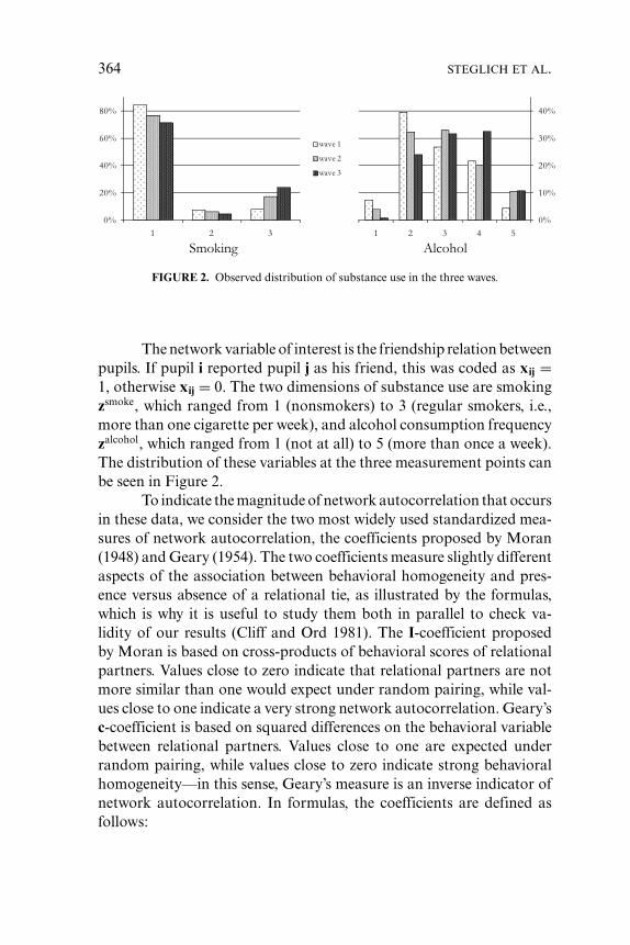
364 STEGLICH ET AL.
FIGURE 2. Observed distribution of substance use in the three waves.
The network variable of interest is the friendship relation betweenpupils. If pupil i reported pupil j as his friend, this was coded as xij =1, otherwise xij = 0. The two dimensions of substance use are smokingzsmoke, which ranged from 1 (nonsmokers) to 3 (regular smokers, i.e.,more than one cigarette per week), and alcohol consumption frequencyzalcohol, which ranged from 1 (not at all) to 5 (more than once a week).The distribution of these variables at the three measurement points canbe seen in Figure 2.
To indicate the magnitude of network autocorrelation that occursin these data, we consider the two most widely used standardized mea-sures of network autocorrelation, the coefficients proposed by Moran(1948) and Geary (1954). The two coefficients measure slightly differentaspects of the association between behavioral homogeneity and pres-ence versus absence of a relational tie, as illustrated by the formulas,which is why it is useful to study them both in parallel to check va-lidity of our results (Cliff and Ord 1981). The I-coefficient proposedby Moran is based on cross-products of behavioral scores of relationalpartners. Values close to zero indicate that relational partners are notmore similar than one would expect under random pairing, while val-ues close to one indicate a very strong network autocorrelation. Geary’sc-coefficient is based on squared differences on the behavioral variablebetween relational partners. Values close to one are expected underrandom pairing, while values close to zero indicate strong behavioralhomogeneity—in this sense, Geary’s measure is an inverse indicator ofnetwork autocorrelation. In formulas, the coefficients are defined asfollows:
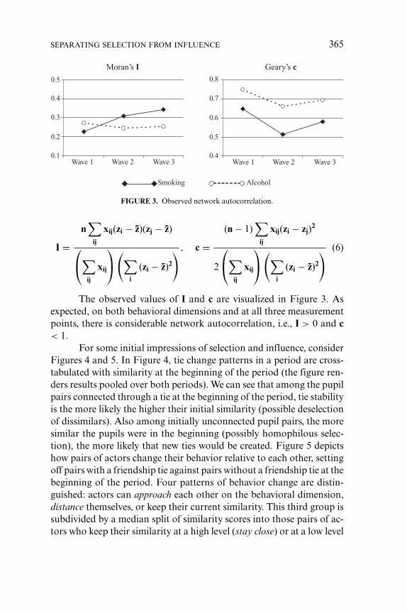
SEPARATING SELECTION FROM INFLUENCE 365
0.1
0.2
0.3
0.4
0.4
0.5
0.6
0.7
0.80.5
Wave 1
Moran’s I Geary’s c
Wave 2 Wave 3
Smoking Alcohol
Wave 1 Wave 2 Wave 3
FIGURE 3. Observed network autocorrelation.
I =n
∑ij
xij(zi − z)(zj − z)
⎛⎝∑
ij
xij
⎞⎠(∑
i
(zi − z)2
) , c =(n − 1)
∑ij
xij(zi − zj)2
2
⎛⎝∑
ij
xij
⎞⎠ (∑
i
(zi − z)2
) (6)
The observed values of I and c are visualized in Figure 3. Asexpected, on both behavioral dimensions and at all three measurementpoints, there is considerable network autocorrelation, i.e., I > 0 and c< 1.
For some initial impressions of selection and influence, considerFigures 4 and 5. In Figure 4, tie change patterns in a period are cross-tabulated with similarity at the beginning of the period (the figure ren-ders results pooled over both periods). We can see that among the pupilpairs connected through a tie at the beginning of the period, tie stabilityis the more likely the higher their initial similarity (possible deselectionof dissimilars). Also among initially unconnected pupil pairs, the moresimilar the pupils were in the beginning (possibly homophilous selec-tion), the more likely that new ties would be created. Figure 5 depictshow pairs of actors change their behavior relative to each other, settingoff pairs with a friendship tie against pairs without a friendship tie at thebeginning of the period. Four patterns of behavior change are distin-guished: actors can approach each other on the behavioral dimension,distance themselves, or keep their current similarity. This third group issubdivided by a median split of similarity scores into those pairs of ac-tors who keep their similarity at a high level (stay close) or at a low level
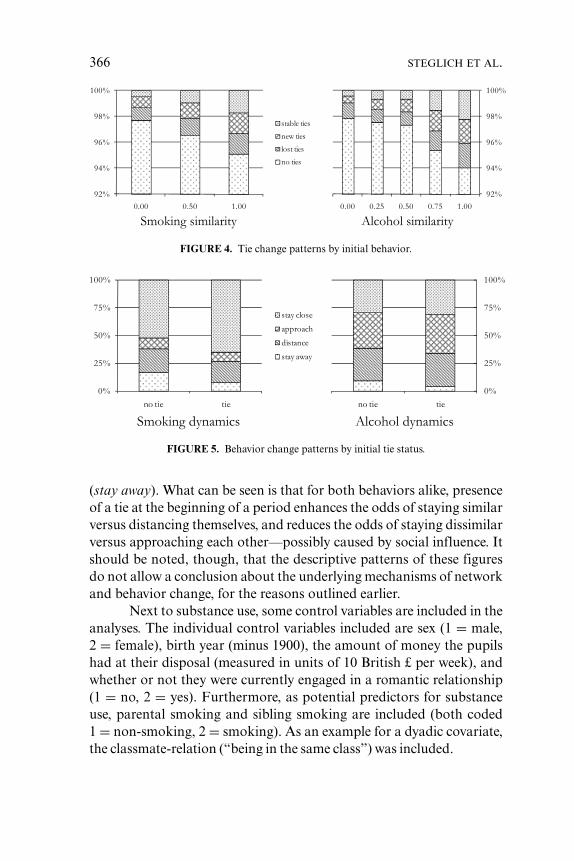
366 STEGLICH ET AL.
FIGURE 4. Tie change patterns by initial behavior.
FIGURE 5. Behavior change patterns by initial tie status.
(stay away). What can be seen is that for both behaviors alike, presenceof a tie at the beginning of a period enhances the odds of staying similarversus distancing themselves, and reduces the odds of staying dissimilarversus approaching each other—possibly caused by social influence. Itshould be noted, though, that the descriptive patterns of these figuresdo not allow a conclusion about the underlying mechanisms of networkand behavior change, for the reasons outlined earlier.
Next to substance use, some control variables are included in theanalyses. The individual control variables included are sex (1 = male,2 = female), birth year (minus 1900), the amount of money the pupilshad at their disposal (measured in units of 10 British £ per week), andwhether or not they were currently engaged in a romantic relationship(1 = no, 2 = yes). Furthermore, as potential predictors for substanceuse, parental smoking and sibling smoking are included (both coded1 = non-smoking, 2 = smoking). As an example for a dyadic covariate,the classmate-relation (“being in the same class”) was included.
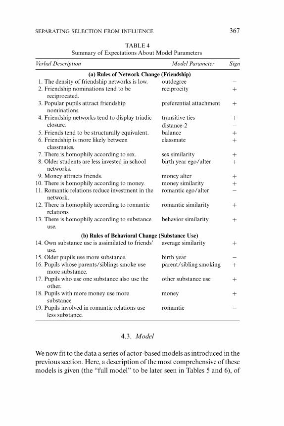
SEPARATING SELECTION FROM INFLUENCE 367
TABLE 4Summary of Expectations About Model Parameters
Verbal Description Model Parameter Sign
(a) Rules of Network Change (Friendship)1. The density of friendship networks is low. outdegree −2. Friendship nominations tend to be
reciprocated.reciprocity +
3. Popular pupils attract friendshipnominations.
preferential attachment +
4. Friendship networks tend to display triadicclosure.
transitive ties +distance-2 −
5. Friends tend to be structurally equivalent. balance +6. Friendship is more likely between
classmates.classmate +
7. There is homophily according to sex. sex similarity +8. Older students are less invested in school
networks.birth year ego/alter +
9. Money attracts friends. money alter +10. There is homophily according to money. money similarity +11. Romantic relations reduce investment in the
network.romantic ego/alter −
12. There is homophily according to romanticrelations.
romantic similarity +
13. There is homophily according to substanceuse.
behavior similarity +
(b) Rules of Behavioral Change (Substance Use)14. Own substance use is assimilated to friends’
use.average similarity +
15. Older pupils use more substance. birth year −16. Pupils whose parents/siblings smoke use
more substance.parent/sibling smoking +
17. Pupils who use one substance also use theother.
other substance use +
18. Pupils with more money use moresubstance.
money +
19. Pupils involved in romantic relations useless substance.
romantic −
4.3. Model
We now fit to the data a series of actor-based models as introduced in theprevious section. Here, a description of the most comprehensive of thesemodels is given (the “full model” to be later seen in Tables 5 and 6), of
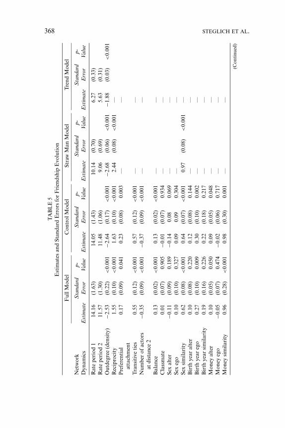
368 STEGLICH ET AL.
TA
BL
E5
Est
imat
esan
dSt
anda
rdE
rror
sfo
rF
rien
dshi
pE
volu
tion
Ful
lMod
elC
ontr
olM
odel
Stra
wM
anM
odel
Tre
ndM
odel
Net
wor
kS
tand
ard
p-S
tand
ard
p-S
tand
ard
p-S
tand
ard
p-D
ynam
ics
Est
imat
eE
rror
Val
ueE
stim
ate
Err
orV
alue
Est
imat
eE
rror
Val
ueE
stim
ate
Err
orV
alue
Rat
epe
riod
114
.16
(1.6
3)14
.05
(1.4
3)10
.14
(0.7
0)6.
27(0
.33)
Rat
epe
riod
211
.57
(1.3
0)11
.48
(1.0
6)9.
06(0
.69)
5.63
(0.3
1)O
utde
gree
(den
sity
)−2
.53
(0.2
2)<
0.00
1−2
.64
(0.1
7)<
0.00
1−2
.68
(0.0
6)<
0.00
1−1
.88
(0.0
3)<
0.00
1R
ecip
roci
ty1.
55(0
.10)
<0.
001
1.63
(0.1
0)<
0.00
12.
44(0
.08)
<0.
001
—P
refe
rent
ial
atta
chm
ent
0.17
(0.0
9)0.
041
0.23
(0.0
8)0.
003
——
Tra
nsit
ive
ties
0.55
(0.1
2)<
0.00
10.
57(0
.12)
<0.
001
——
Num
ber
ofac
tors
atdi
stan
ce2
−0.3
5(0
.09)
<0.
001
−0.3
7(0
.09)
<0.
001
——
Bal
ance
0.13
(0.0
2)<
0.00
10.
13(0
.02)
<0.
001
——
Cla
ssm
ate
0.01
(0.0
7)0.
905
−0.0
1(0
.07)
0.93
4—
—Se
xal
ter
−0.1
1(0
.09)
0.18
9−0
.14
0.08
0.06
9—
—Se
xeg
o0.
10(0
.10)
0.32
70.
090.
090.
304
——
Sex
sim
ilari
ty0.
62(0
.08)
<0.
001
0.64
(0.0
7)<
0.00
10.
97(0
.08)
<0.
001
—B
irth
year
alte
r0.
10(0
.08)
0.22
00.
12(0
.08)
0.14
4—
—B
irth
year
ego
0.27
(0.1
0)0.
009
0.30
(0.1
0)0.
002
——
Bir
thye
arsi
mila
rity
0.19
(0.1
6)0.
226
0.22
(0.1
8)0.
217
——
Mon
eyal
ter
0.10
(0.0
5)0.
050
0.09
(0.0
5)0.
048
——
Mon
eyeg
o−0
.05
(0.0
7)0.
474
−0.0
2(0
.06)
0.71
7—
—M
oney
sim
ilari
ty0.
96(0
.28)
<0.
001
0.98
(0.3
0)0.
001
——
(Con
tinu
ed)
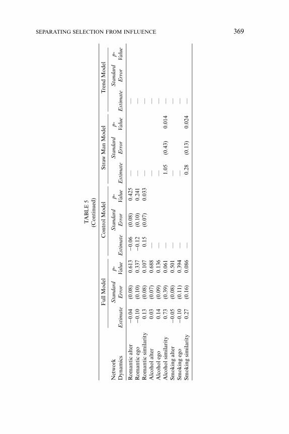
SEPARATING SELECTION FROM INFLUENCE 369
TA
BL
E5
(Con
tinu
ed)
Ful
lMod
elC
ontr
olM
odel
Stra
wM
anM
odel
Tre
ndM
odel
Net
wor
kS
tand
ard
p-S
tand
ard
p-S
tand
ard
p-S
tand
ard
p-D
ynam
ics
Est
imat
eE
rror
Val
ueE
stim
ate
Err
orV
alue
Est
imat
eE
rror
Val
ueE
stim
ate
Err
orV
alue
Rom
anti
cal
ter
−0.0
4(0
.08)
0.61
3−0
.06
(0.0
8)0.
425
——
Rom
anti
ceg
o−0
.10
(0.1
0)0.
337
−0.1
2(0
.10)
0.24
1—
—R
oman
tic
sim
ilari
ty0.
13(0
.08)
0.10
70.
15(0
.07)
0.03
3—
—A
lcoh
olal
ter
0.03
(0.0
7)0.
688
——
—A
lcoh
oleg
o0.
14(0
.09)
0.13
6—
——
Alc
ohol
sim
ilari
ty0.
73(0
.39)
0.06
1—
1.05
(0.4
3)0.
014
—Sm
okin
gal
ter
−0.0
5(0
.08)
0.50
1—
——
Smok
ing
ego
−0.1
0(0
.11)
0.39
4—
——
Smok
ing
sim
ilari
ty0.
27(0
.16)
0.08
6—
0.28
(0.1
3)0.
024
—
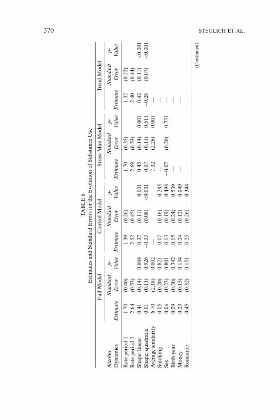
370 STEGLICH ET AL.
TA
BL
E6
Est
imat
esan
dSt
anda
rdE
rror
sfo
rth
eE
volu
tion
ofSu
bsta
nce
Use
Ful
lMod
elC
ontr
olM
odel
Stra
wM
anM
odel
Tre
ndM
odel
Alc
ohol
Sta
ndar
dp-
Sta
ndar
dp-
Sta
ndar
dp-
Sta
ndar
dp-
Dyn
amic
sE
stim
ate
Err
orV
alue
Est
imat
eE
rror
Val
ueE
stim
ate
Err
orV
alue
Est
imat
eE
rror
Val
ue
Rat
epe
riod
11.
70(0
.40)
1.39
(0.2
6)1.
70(0
.35)
1.32
(0.2
2)R
ate
peri
od2
2.64
(0.5
3)2.
52(0
.45)
2.69
(0.5
3)2.
40(0
.44)
Shap
e:lin
ear
0.41
(0.1
4)0.
004
0.37
(0.1
1)0.
001
0.45
(0.1
4)0.
001
0.42
(0.1
1)<
0.00
1Sh
ape:
quad
rati
c0.
01(0
.11)
0.92
6−0
.33
(0.0
8)<
0.00
10.
07(0
.11)
0.51
1−0
.28
(0.0
7)<
0.00
1A
vera
gesi
mila
rity
6.70
(2.1
8)0.
002
—7.
32(2
.26)
0.00
1—
Smok
ing
0.05
(0.2
0)0.
821
0.17
(0.1
6)0.
285
——
Sex
0.06
(0.2
3)0.
801
0.13
(0.1
9)0.
498
−0.0
7(0
.20)
0.73
1—
Bir
thye
ar0.
29(0
.30)
0.34
20.
15(0
.24)
0.53
9—
—M
oney
0.23
(0.1
5)0.
134
0.24
(0.1
2)0.
049
——
Rom
anti
c−0
.45
(0.3
2)0.
151
−0.2
5(0
.26)
0.34
4—
—
(Con
tinu
ed)
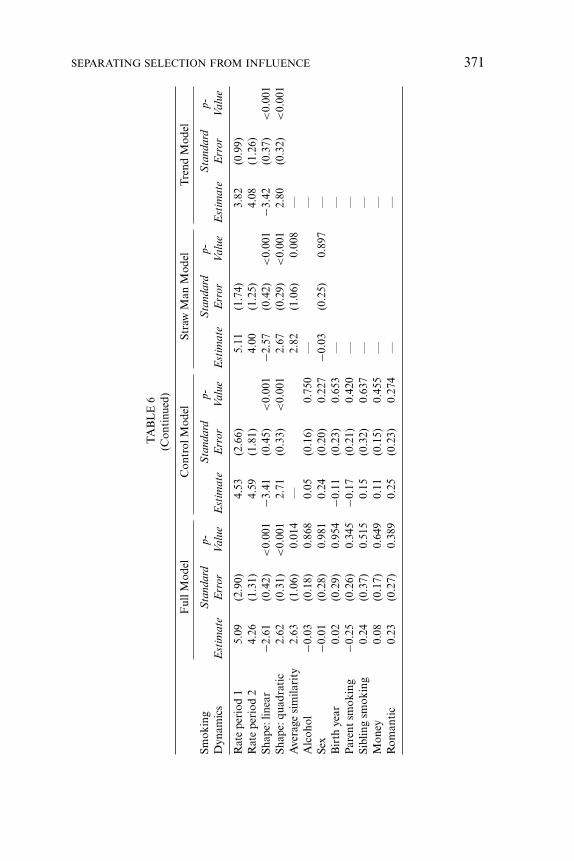
SEPARATING SELECTION FROM INFLUENCE 371
TA
BL
E6
(Con
tinu
ed)
Ful
lMod
elC
ontr
olM
odel
Stra
wM
anM
odel
Tre
ndM
odel
Smok
ing
Sta
ndar
dp-
Sta
ndar
dp-
Sta
ndar
dp-
Sta
ndar
dp-
Dyn
amic
sE
stim
ate
Err
orV
alue
Est
imat
eE
rror
Val
ueE
stim
ate
Err
orV
alue
Est
imat
eE
rror
Val
ue
Rat
epe
riod
15.
09(2
.90)
4.53
(2.6
6)5.
11(1
.74)
3.82
(0.9
9)R
ate
peri
od2
4.26
(1.3
1)4.
59(1
.81)
4.00
(1.2
5)4.
08(1
.26)
Shap
e:lin
ear
−2.6
1(0
.42)
<0.
001
−3.4
1(0
.45)
<0.
001
−2.5
7(0
.42)
<0.
001
−3.4
2(0
.37)
<0.
001
Shap
e:qu
adra
tic
2.62
(0.3
1)<
0.00
12.
71(0
.33)
<0.
001
2.67
(0.2
9)<
0.00
12.
80(0
.32)
<0.
001
Ave
rage
sim
ilari
ty2.
63(1
.06)
0.01
4—
2.82
(1.0
6)0.
008
—A
lcoh
ol−0
.03
(0.1
8)0.
868
0.05
(0.1
6)0.
750
——
Sex
−0.0
1(0
.28)
0.98
10.
24(0
.20)
0.22
7−0
.03
(0.2
5)0.
897
—B
irth
year
0.02
(0.2
9)0.
954
−0.1
1(0
.23)
0.65
3—
—P
aren
tsm
okin
g−0
.25
(0.2
6)0.
345
−0.1
7(0
.21)
0.42
0—
—Si
blin
gsm
okin
g0.
24(0
.37)
0.51
50.
15(0
.32)
0.63
7—
—M
oney
0.08
(0.1
7)0.
649
0.11
(0.1
5)0.
455
——
Rom
anti
c0.
23(0
.27)
0.38
90.
25(0
.23)
0.27
4—
—
372 STEGLICH ET AL.
which all the other models are simplifications. The model for friendshipdynamics is first discussed by specifying the network objective functionand then the behavior objective functions are sketched, one for eachtype of substance use, modeling behavior dynamics.
An overall tendency to form network ties, expressed by the out-degree effect, forms the basis of the network objective function. It isexpected to be negative due to the low density of the observed networks(see the first row in Table 2). Endogenous determinants of networkevolution are properties by which the network, in a feedback process,affects its own dynamics. We include several endogenous network ef-fects: the tendency to reciprocate friendship nominations (reciprocityeffect, expected positive, second row in Table 2), the tendency to nom-inate popular (i.e., frequently chosen) others as friends (“preferentialattachment,” expected positive, third row), and tendencies toward net-work closure and structural balance. Network closure means that directfriendship relations are more likely to those others who also indirectlyare friends—that is, who are linked via a third pupil. This could be op-erationalized by three different effects, described in rows 4–6 of Table2, of which we chose rows 5 and 6. Structural balance is a well-knownconcept dating back to Heider (1958). In our operationalization (row7), we measure it by the tendency to be friends with pupils who share thesame other friends: the more similar the friendship selection patternsof two pupils (in network jargon: the more structurally equivalent theyare), the more likely they are to also choose each other as friends. Otherendogenous network effects that could be included in a model, butwhich we omitted for lack of substantive theory in the present case, arerelated to hierarchization and brokerage. An aversion to forming three-cycles indicates the presence of an informal hierarchy in the networkand could be modeled by including the corresponding effect (row 8).The betweenness effect (row 9) measures a tendency to assume a brokerrole in the friendship network by establishing indirect links between net-work regions that are not directly connected. For friendship networks,it can be expected that there is no hierarchy and that brokerage playslittle role, hence our omission of these effects.
The dyadic variable wclassmate, indicating whether two pupils be-long to the same class in the cohort, is expected to have a main (pos-itive) effect on friendship, which is included in the model as a statis-tic
∑j xijwclassmate
ij (not visualized in Table 2). The individual variablessex, birth year, money, and involvement in romantic relations can be
SEPARATING SELECTION FROM INFLUENCE 373
expected to affect friendship evolution in three ways: as a main effect onalter attractiveness (row 10), as a main effect on network activity of ego(row 11), and as a similarity effect of homophilous selection (row 12).Finally, in order to assess the effects of selection based on substanceuse, also taking into account the variables smoking and alcohol use, theego-, alter-, and similarity effects are included in the model specifica-tion. In part (a) of Table 4, reasonable expectations about the signs ofsome effects are given. Because for our purpose most effects play onlythe auxiliary role of control variables, we do not discuss them furtherhere. Nonetheless, their inclusion is crucial for our aim of explainingnetwork autocorrelation and properly separating selection and influ-ence, as they capture the “alternative generating mechanisms” that weidentified as a key issue to take into account.
The basis for modeling the evolution of the substance use di-mensions are two parameters expressing the shape of the variables’ dis-tributions in the long run. Looking again at Figure 2, the distributionof the smoking variable is U-shaped, while the alcohol consumptionvariable is distributed according to an inverse U-shape. In the objec-tive function, these different shapes can be expressed by the linear andquadratic effects of substance use (see the first row in Table 3). Thesign of the quadratic term here indicates whether the objective functionis a parabola opening upward (a positive sign, implying a U-shapeddistribution as observed for the smoking variable) or downward (a neg-ative sign, implying an inverse U-shaped distribution as observed forthe alcohol variable).
For measuring social influence on substance use, different oper-ationalizations are possible, such as an effect of average similarity toneighbors (second row), an effect of similarity that is not averaged butis added over neighbors (third row), or a main effect of peers’ averagesubstance use (row 4). Which of those, if any, is best-suited for modelingsocial influence remains in principle an empirical question. Based onscore-type tests (Schweinberger 2004) that provide a statistical basis forchoosing between such alternative operationalizations, we here chosethe average similarity effect, as it fit best with our data. It also corre-sponds most closely to the intuitive idea that each pupil is influencedby his group of friends in about the same way (Cohen 1977).
Individual variables v (e.g., sibling smoking) are included asmain effects in the behavior objective functions, i.e., with statistics(zi − z)(vi − v) (not visualized in Table 3), reflecting (if the coefficient
374 STEGLICH ET AL.
is positive) that higher values of v will tend to lead to higher values ofz. In the same way, the main effect of the substance use dimensions oneach other can also be included. Part (b) in Table 4 gives an overview ofreasonable expectations concerning the specific model parameters forthe substance use dynamics.
4.4. Results
We estimated models of four degrees of complexity for the coevolutionof the friendship network with smoking behavior and alcohol consump-tion. The trend model postulates purely random change of network andbehavior, and the control model contains all effects except selection andinfluence related to the behavioral variables. These models will furtherserve as benchmarks for explaining observed network autocorrelation inthe discussion below. The full model is the one in which the hypothesesfrom Table 4 are tested. The straw man model, finally, is a deliberatelymis-specified model in which selection and influence are modeled ina “naive” way—that is, not controlling for most of the effects in thecontrol model. This straw man will serve for illustrating the dangers ofmodel mis-specification, in terms of failure to control for alternativegenerating mechanisms. Tables 5 and 6 give parameter estimates for themodels discussed below.
First the network evolution part is considered (reported inTable 5) and then the evolution of the two behavioral dimensions smok-ing and alcohol consumption (reported in Table 6). The parametersof main interest for friendship dynamics are those that operational-ize friend selection based on substance use. The ego- and alter effectsof this type do not reach significance, suggesting that there is not amain effect of substance use on either friendship nominating activ-ity or on popularity in the network. The homophily-operationalizingparameters have the predicted sign but are only marginally signifi-cant (parameters alcohol similarity and smoking similarity in row 13 ofTable 4). This indicates that the descriptive evidence for homophilous se-lection according to substance use (Figure 4) cannot be fully attributedto a genuine homophilous selection mechanism, but in part also resultsfrom a combination of mechanisms expressed by the other parame-ters. A look at the straw man model’s estimates confirms this impres-sion: when not comprehensively controlling for alternative generating
SEPARATING SELECTION FROM INFLUENCE 375
mechanisms, much stronger test results for homophily based on sub-stance use are found—a result not to be taken seriously. Effects that aremore likely responsible for the appearance of significant homophily inthe straw man model are those that are significant in the full model butnot included in the straw man model.
The inherent tendency of friendship to be reciprocated, a ten-dency toward seeking popular others as friends, network closure, andstructural balance, together constitute a highly significant endogenousexplanation of observed friendship dynamics. The corresponding pa-rameters’ signs confirm our expectations formulated in Table 4 (param-eters outdegree through balance in Table 5; expectations 1 through 5in Table 4). Also among the covariate effects, several expectations canbe confirmed, such as strong homophily mechanisms based on sex andmoney (parameters sex similarity and money similarity; expectations 7and 10 in Table 4), a marginal homophily effect of having a romanticrelation (parameter romantic similarity; expectation 12), higher attrac-tiveness of rich versus poor friends (parameter money alter; expectation9), and a lower network presence of older pupils, as expressed in thepositive ego effect of birth year (parameter birth year ego; expectation8; the alter effect of birth year fell short of significance). Expectationsthat cannot be confirmed are those about lower friendship involvementof students with romantic relations (parameters romantic ego & alter;expectation 11), and—surprisingly—also the classmate effect (param-eter classmate; expectation 6). This may be due to the fact that in theschool studied, teaching at the time did not take place in a classroomcontext, but in courses of varying composition. The class was a largelyadministrative unit and did not necessarily reflect opportunity for socialinteraction.
The behavioral evolution part of the models consists of the sub-models for smoking dynamics and alcohol dynamics, with the resultsreported in Table 6. Here, the focus of interest is on social influencemechanisms (expectation 14 in Table 4), and these are clearly confirmedby our analyses—the average similarity parameter indicates strong as-similation effects on both substance use dimensions, in the full modeland in the straw man model alike. The overall consistency between thesetwo models indicates that the mechanisms of behavior change that wecontrol for seem to be less related to social influence processes.
The two shape parameters of the smoking submodel confirm theexpectation of a U-shaped basis for the objective function, which holds
376 STEGLICH ET AL.
for all estimated models alike. This suggests that this empirical shape(see again Figure 2) does not result from influence mechanisms alone,but might express a “universal” property of smoking. There hardlyseems to be a “middle ground”, and pupils are either nonsmokers orregular smokers, possibly reflecting addiction effects. Social influenceexists but is unlikely to override this basic pattern. For alcohol con-sumption, the expected inverse U-shape is only found back in the sim-pler models (trend and control) but not in the models containing theassimilation effect. Apparently, the inverse U-shape of the empiricaldistributions of alcohol use in Figure 2 can be better explained as re-sulting from assimilation to friends’ alcohol consumption than from auniversal, network-independent shape of the distribution. Recall in thiscontext that the modeling conditions on the first observation. The in-verse U-shaped distribution of alcohol scores that already exists at thisfirst observation moment is therefore not explained, but its persistenceover time is sufficiently explained as resulting from assimilation to net-work neighbors. Finally, none of the included covariates (expectations15–19 in Table 4) significantly explains the evolution of either substanceuse dimension, stressing the point that alternative generating mecha-nisms seem not to play as strong a role on the substance use dimensionsas they did on the network dimension.
4.5. Conclusions from the Analyses
Proceeding from these results, we can now draw conclusions aboutwhich of the mentioned theories are able to account for the observedcoevolution dynamics. The dynamics of smoking behavior and alcoholconsumption follow roughly the same patterns: for both substances, theparameters for homophilous selection and for assimilation are signifi-cant. Based on significance of effects, the results in the first place canbe viewed as a confirmation of social influence theories. However, theevidence for alcohol consumption being a “social phenomenon” in thesense of pupils being influenced by their friends is stronger than forsmoking, which can be derived from calculation of odds as well as fromparameter significance (p = 0.002 versus p = 0.014). A micro step onthe alcohol dimension toward the friends’ average alcohol use corre-sponds to a change of 1/range(alcohol) = 1/4 in the average similaritystatistic, so the relevant odds of the effect are exp(6.7/4) = 5.3. For the

SEPARATING SELECTION FROM INFLUENCE 377
corresponding effect in smoking dynamics, the odds are exp(2.63/2) =3.7. Also, the quadratic shape parameter for smoking remains signifi-cant and is positive in the full model, unlike for alcohol, which suggeststhat an important part is played by the addictive nature of smoking,which may override social influence.
Selection of friends may well lead to friendship between pupilsof similar substance use, as can be seen from the straw man model(p = 0.014 for alcohol, p = 0.024 for smoking). However, this by andlarge seems not to result from genuine homophily according to thesesubstance use patterns, but from other, significant selection patternsthat are controlled for, as the significance drops to marginal size (p =0.061 for alcohol, p = 0.086 for smoking) when we control for a broadarray of alternative mechanisms of friendship formation, as is donein the full model. So, in the second place, the results can be seen assupporting the argument in Feld (1981, 1982) about similarity resultingfrom context effects rather than occurring independently from those.In order to show the validity of this argument, however, it needs to beinvestigated whether these significant alternative mechanisms do indeedimply similarity on the substance use dimensions—that is, do contributeto network autocorrelation. To test this, we now conduct a simulationstudy.
4.6. A Quantitative Assessment of the Determinants of NetworkAutocorrelation
We now address the issue of measuring the “amount” of network au-tocorrelation allocated by a fitted model to the different generativeprocesses—that is, to selection, influence, and the control processesunrelated to these two main effects. Two alternative measures of net-work autocorrelation are considered, Moran’s I-coefficient and Geary’sc-coefficient, as introduced above. Our overall conclusions from theseanalyses should not depend on the specific measure chosen. We do,however, expect minor quantitative differences since the calculation ofGeary’s measure is based on distances on the substance use scale, whilefor Moran’s coefficient, it is based on cross-products.
The procedure followed is similar in underlying intuition toKandel’s (1978, p 433) quantification proposal, which in a footnoteshe attributes to James Coleman. Also Fisher and Bauman’s (1988)
378 STEGLICH ET AL.
proposal follows the same ideas, so our own proposal in principle isnothing new. Kandel’s procedure was as follows: two simple modelsare first fitted to the data, one operationalizing the selection process“alone,” the other the influence process “alone”. Both models are thenused for calculating expected network autocorrelation, and this cal-culated value indicates the magnitude of the effect considered. Ourimplementation differs from those by Kandel and by Fisher and Bau-man mainly by the fact that we use a model where the selection andinfluence effects are mutually controlled for each other and for othermechanisms. We thus evaluate the observed network autocorrelation,the network autocorrelation implied by our fitted model (explained au-tocorrelation), and the values implied by simpler models, in which eitherselection, or influence, or both, are “switched off.” For this purpose,we combine results from the full and the control model. In addition,in order to assess the amount of network autocorrelation that can beattributed to alternative (“control”) mechanisms, we consider implica-tions of the trend model. In this model, both the selection and influenceeffects as well as the control effects are “switched off”, enabling us toimprove on a second major criticism we had of the earlier studies—namely, their neglect of assessing the impact of alternative mechanisms.The resulting allocation of explained network autocorrelation accord-ing to generating mechanisms can be seen in Figure 6. In these diagrams,it needs to be understood that the pie slices labeled “selection” coversubstance-use based selection only—that is, homophily, ego,- and alter-effects based on substance use. Other selection effects, such as closureor covariate-based homophily, are allocated to the “control” slices.
The percentages in this figure were obtained in the following way.The trend model, the control model, and the full model as well as twohybrid models were used for simulating in continuous time network-behavioral coevolution trajectories that follow the rules extracted fromthe data. Each such trajectory starts out at the first observation ofnetwork and behavior at t1. In the simulations, when time reaches themoment t2 of the second observation, the autocorrelation measure isevaluated on the simulated data. The same procedure is repeated forall periods until the time reaches the last observation moment tM (hereM = 3). This way, observed autocorrelation measures can be relatedto a distribution of simulated autocorrelation measures, and differentmodels can be compared on their implied distributions of networkautocorrelation measures. For brevity, we report only across-period
SEPARATING SELECTION FROM INFLUENCE 379
FIGURE 6. Model-based decomposition of network autocorrelation. Slice sizes correspondto percentages of the coefficient size difference between average predictions ofnull and full models that through simulations could be allocated to differentcoevolution mechanisms.
averages on the network autocorrelation measures. Thus, the variablesstudied in Figure 6 are Moran’s I-coefficient and Geary’s c-coefficient,averaged over observation moments t2 and t3.
The calculations rely on 1000 independent trajectories of thenetwork-behavioral coevolution process of five models. The main modelof interest here is the one in which, next to the control effects, both themain influence effect and the main selection effect were estimated fromthe data (the full model). The model without influence or selection,in which the network and the two behavioral dimensions evolve inde-pendently, is the control model. To assess the impact of the controleffects on the network autocorrelation, the trend model is estimated. Itcontains only the outdegree parameter in the network part and the twoshape parameters in the behavioral parts, and yields network autocorre-lation values that depend on universal trend together with the initiallyobserved state. These three data-fitted models are complemented by
380 STEGLICH ET AL.
TABLE 7Model-Based Simulated Network Autocorrelation
Smoking Alcohol
Model Moran Geary Model Moran Geary
Null −0.007 1.000 Null −0.007 1.000Trend 0.046 (0.049) 0.908 (0.067) Trend 0.024 (0.055) 0.968 (0.071)Control 0.097 (0.064) 0.823 (0.084) Control 0.057 (0.066) 0.930 (0.082)No influence 0.166 (0.064) 0.680 (0.082) No influence 0.143 (0.067) 0.799 (0.077)No selection 0.201 (0.075) 0.733 (0.082) No selection 0.200 (0.079) 0.785 (0.083)Full 0.272 (0.076) 0.598 (0.083) Full 0.301 (0.082) 0.648 (0.077)
Observed 0.310 0.542 Observed 0.247 0.696
two “cross-combined” hybrid models. In one of these, the network partis taken from the full model while the behavioral parts are taken fromthe control model, and in the other one, the combination is reversed.The idea behind this cross-combination is that, in order to identify themagnitude of network autocorrelation explained by only the main se-lection effect, we wish to compare network autocorrelation under thefull model (where selection is controlled for influence) with networkautocorrelation under a model where no selection occurs, while influ-ence resembles that under the full model, and all control effects in thenetwork part fit the data best.
Table 7 renders averages and standard deviations of the networkautocorrelation coefficients over the 1000 simulated network trajecto-ries per model, next to the expected value under permutations of theactors (row “null”) and the observed value. The numbers refer to thecoefficients’ average over t2 and t3, the time points at the end of thetwo periods in which unobserved change is simulated. What needs tobe noticed first is that the values for the full model do not perfectlyfit the observed values. For smoking, the model-predicted values areless extreme than observed, while for alcohol consumption, it is theother way round. This suggests that factors that lie outside the scopeof our models probably enhance smoking autocorrelation, while theyprobably reduce alcohol autocorrelation.
Table 7 clearly shows that the less complex a model is, the lessnetwork autocorrelation it implies. Taking the difference between thefull model’s predictions and the null expectations under independenceas 100% (“all the model explains”), the values of this table were trans-formed into percentages to arrive at the diagrams in Figure 6. Themodels trend, control and full, are hierarchically nested, which meansthat the coefficients can be linearly transformed into percentages. The
SEPARATING SELECTION FROM INFLUENCE 381
other two models, in which either selection or influence are switchedoff, are nested in-between the control and the full model but not withineach other. Therefore, the allocation of percentage values to influenceand homophilous selection can be done in two ways: by considering theincrease of the predicted coefficient upon including the effect, comparedto the control model, or by considering the decrease of the predictedcoefficient upon excluding the effect, compared to the full model. Theresulting discrepancy of both calculations is rendered as “indetermi-nate” in the diagrams.
As suspected, trend and control effects are responsible for a con-siderable part of the observed network autocorrelation. More than one-third of the explained autocorrelation on smoking is epiphenomenal—that is, resulting from processes other than substance use based selectionand the social influence of school friends. For alcohol consumption, therole of these effects is much weaker, approximately one-fifth of the totalexplained autocorrelation. The fractions that are allocated to influenceand selection processes show two main results. On the one hand, there isa systematic difference between substance use dimensions. For alcoholuse, the contribution of influence effects relative to selection effects isstronger than for tobacco use, where selection plays a more importantrole. On the other hand, there is a systematic difference between the twoautocorrelation coefficients. Moran’s I identifies an overall stronger roleof influence mechanisms than does Geary’s c. For smoking, this discrep-ancy is even so strong that the two coefficients suggest opposite answersto the question asking which of the two mechanisms contributes mostto autocorrelation.
In order to understand this discrepancy, we take a closer lookat the mathematical relationship between the two autocorrelation co-efficients. Making use of (6), the Geary coefficient can be expresseddepending on the Moran coefficient, as follows
c = (1 − n)n
I +(n − 1)
∑i
(xi+ + x+i)(zi − z)2
2
⎛⎝∑
ij
xit
⎞⎠ (∑
i
(zi − z)2
) (7)
where xi+ and x+i stand for actor i’s outdegree and indegree, respectively,and their sum can be seen as the actor’s overall connectedness. The termby which the two autocorrelation coefficients differ is proportional to
382 STEGLICH ET AL.
∑i (xi+ + x+i)(zi − z)2, the connectedness-weighted sum of squared dis-
tances from the behavioral average. What (7) implies is on the one handthat for data sets in which the highly connected actors are behaviorallyextreme, the two coefficients give qualitatively different results, whilefor data sets in which they are behaviorally average, the coefficients giveidentical results. In our data (see again Figure 2), the smoking variablehas a U-shaped distribution, so we can expect strong differences. Thealcohol variable is unimodally distributed, which means that differencesshould be smaller. In fact, this pattern is what we observe in Figure 6.On the other hand, (7) implies that the Geary coefficient de-emphasizesthe contribution of behaviorally extreme actors compared to the Morancoefficient (recall that Geary’s c is an inverse measure of network au-tocorrelation). Any difference between the decomposition results forthe two coefficients can therefore be interpreted as resulting from thisdifferent emphasis.
Given these considerations, we must come to the following con-clusions: While there is significant evidence for assimilation to friendson both substance use dimensions, this influence effect seems to occurmore strongly in the behaviorally extreme groups, because Moran’s co-efficient (which is more sensitive to the contribution of these groups)identifies an overall stronger role of influence. For smoking, these ex-treme groups are the majority of students (U-shape of the distribution),which explains why the discrepancy of decomposition results betweenautocorrelation coefficients is particularly strong. For alcohol use, theextreme groups constitute a minority (inverse U-shape), hence the dis-crepancy of results is smaller.
5. DISCUSSION
In this paper, we presented a new method for analyzing the coevolu-tion of social networks and changing characteristics of the actors inthe network. The method is based on an explicit probability model forchanges in network ties and individual behavior, mutually reacting onone another. This coevolution is crucial for a variety of research topicsthat currently receive a lot of attention. Examples are studies aboutthe spread of health-related behaviors, like the smoking and drinkingbehavior studied in our example, about the spread of deviance andcrime, about the effects of communication interaction on individual
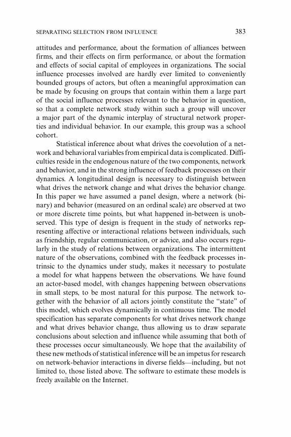
SEPARATING SELECTION FROM INFLUENCE 383
attitudes and performance, about the formation of alliances betweenfirms, and their effects on firm performance, or about the formationand effects of social capital of employees in organizations. The socialinfluence processes involved are hardly ever limited to convenientlybounded groups of actors, but often a meaningful approximation canbe made by focusing on groups that contain within them a large partof the social influence processes relevant to the behavior in question,so that a complete network study within such a group will uncovera major part of the dynamic interplay of structural network proper-ties and individual behavior. In our example, this group was a schoolcohort.
Statistical inference about what drives the coevolution of a net-work and behavioral variables from empirical data is complicated. Diffi-culties reside in the endogenous nature of the two components, networkand behavior, and in the strong influence of feedback processes on theirdynamics. A longitudinal design is necessary to distinguish betweenwhat drives the network change and what drives the behavior change.In this paper we have assumed a panel design, where a network (bi-nary) and behavior (measured on an ordinal scale) are observed at twoor more discrete time points, but what happened in-between is unob-served. This type of design is frequent in the study of networks rep-resenting affective or interactional relations between individuals, suchas friendship, regular communication, or advice, and also occurs regu-larly in the study of relations between organizations. The intermittentnature of the observations, combined with the feedback processes in-trinsic to the dynamics under study, makes it necessary to postulatea model for what happens between the observations. We have foundan actor-based model, with changes happening between observationsin small steps, to be most natural for this purpose. The network to-gether with the behavior of all actors jointly constitute the “state” ofthis model, which evolves dynamically in continuous time. The modelspecification has separate components for what drives network changeand what drives behavior change, thus allowing us to draw separateconclusions about selection and influence while assuming that both ofthese processes occur simultaneously. We hope that the availability ofthese new methods of statistical inference will be an impetus for researchon network-behavior interactions in diverse fields—including, but notlimited to, those listed above. The software to estimate these models isfreely available on the Internet.
384 STEGLICH ET AL.
Important scholarly work has been published in the econometricliterature about the difficulty of identifying endogenous social interac-tions, defined by Manski (1993: 532) as effects “wherein the propensityof an individual to behave in some way varies with the behavior ofthe group.” Our model presents a special case of endogenous socialinteractions, where the group is defined as the personal network (thecollection of members of the total network to whom the focal actorhas an outgoing tie) and determined endogenously. In this case, it ispossible to obtain meaningful estimates of these effects, due to the lon-gitudinal design, the observation of the ties in the network, and themodel assumptions being postulated.
As in any statistical model, the validity of the conclusions de-pends on the tenability of the model as, at least, an adequate approxima-tion. A crucial assumption in our general modeling approach is that theprobabilities of the changes in network and behavior depend only on thecurrent value of network and behavior (the “state” of the model) and onthe observed exogenous actor-bound and dyadic variables—in mathe-matical terms, that network and behavior jointly evolve as a Markovprocess (Norris 1997). Making such an assumption for modeling net-work dynamics was first proposed by Holland and Leinhardt (1977),and our approach shares this assumption with many actor-based mod-els as well as with many statistical models. It should be noted that it isnot assumed that the observed system is in equilibrium. The specifica-tion of the objective functions (cf. Tables 2 and 3) offers much flexibilityto specify how exactly the probabilities of change depend on the cur-rent state and the independent variables, while staying within the classof Markov processes. In the empirical analyses, we therefore includeda relatively large number of independent variables—to obtain a goodfit between model and data, and to alleviate concerns about the modelassumptions.
In the empirical part of the paper, we showed how persistentpuzzles surrounding network autocorrelation in substance use amongadolescents could be solved for the case of a study of a secondaryschool cohort in Glasgow by applying our method. We showed that inour data set, there was evidence for peer influence on both substanceuse dimensions, stronger for alcohol consumption but still significantfor smoking. The effects of partner selection, on the other hand, wereidentified to be only weakly related to substance use, hinging more onmechanisms of network closure, structural balance, and selection based
SEPARATING SELECTION FROM INFLUENCE 385
on sociodemographic properties. Simulation studies served to quantifythe “amount” of network autocorrelation that could be ascribed to thedifferent processes of trend (in behavior and network evolution), controlmechanisms, substance use based selection, and influence. These studiesserved to improve on earlier, similar attempts in the literature, in whichthe role of trend and control mechanisms in particular was neglected,and which arrived at diverging conclusions about the importance ofselection and influence effects.
Important remaining concerns are the possibility of observationerrors, the problem of correlated unobservables (Moffitt 2001; Mouw2006), and the possibility of dependence on past events. These issueswill hopefully be treated in future work, and we only briefly discuss eachof them here. The first concern is that observation errors are a blindspot in available methods for social network analysis. Although muchis known about inaccuracies in social network observations (Marsden2005), most or all currently available statistical analysis methods assumethat observation is perfect. This will be an important area for furthermethodological developments.
The second important concern is the possibility that there maybe nonobserved variables codetermining the probabilities of change innetwork and/or behavior. These variables should then be added to thestate variable of the system in order to satisfy the Markov property.This problem is recognized in a wide variety of models as the endogene-ity of important explanatory variables (Manski 1993; Moffitt 2001).The royal road to solving it is the development of better theory andmore extensive data collection. An advantage of linear models, com-pared to models for discrete data like ours, is the availability of methodssuch as fixed effects that may control, under suitable assumptions, forunobserved time-constant actor differences (Mouw 2006). Such meth-ods have not yet been developed for the model presented in this pa-per. This concern implies for our approach that conclusions should bephrased cautiously, without strict causal interpretations. An example ofcorrelated unobservables in our setup would be the possible existenceof an unobserved individual characteristic v with the properties that attime tA individuals make enduring ties mainly to others with similarvalues on v, while at time tB individuals change their value on the be-havioral variable z depending on their v values. If tA < tB, the processwill seem to be influence (persons who are tied become similar on z),whereas if tA > tB, the process will seem to be selection (persons who
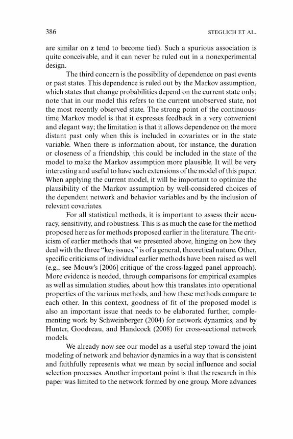
386 STEGLICH ET AL.
are similar on z tend to become tied). Such a spurious association isquite conceivable, and it can never be ruled out in a nonexperimentaldesign.
The third concern is the possibility of dependence on past eventsor past states. This dependence is ruled out by the Markov assumption,which states that change probabilities depend on the current state only;note that in our model this refers to the current unobserved state, notthe most recently observed state. The strong point of the continuous-time Markov model is that it expresses feedback in a very convenientand elegant way; the limitation is that it allows dependence on the moredistant past only when this is included in covariates or in the statevariable. When there is information about, for instance, the durationor closeness of a friendship, this could be included in the state of themodel to make the Markov assumption more plausible. It will be veryinteresting and useful to have such extensions of the model of this paper.When applying the current model, it will be important to optimize theplausibility of the Markov assumption by well-considered choices ofthe dependent network and behavior variables and by the inclusion ofrelevant covariates.
For all statistical methods, it is important to assess their accu-racy, sensitivity, and robustness. This is as much the case for the methodproposed here as for methods proposed earlier in the literature. The crit-icism of earlier methods that we presented above, hinging on how theydeal with the three “key issues,” is of a general, theoretical nature. Other,specific criticisms of individual earlier methods have been raised as well(e.g., see Mouw’s [2006] critique of the cross-lagged panel approach).More evidence is needed, through comparisons for empirical examplesas well as simulation studies, about how this translates into operationalproperties of the various methods, and how these methods compare toeach other. In this context, goodness of fit of the proposed model isalso an important issue that needs to be elaborated further, comple-menting work by Schweinberger (2004) for network dynamics, and byHunter, Goodreau, and Handcock (2008) for cross-sectional networkmodels.
We already now see our model as a useful step toward the jointmodeling of network and behavior dynamics in a way that is consistentand faithfully represents what we mean by social influence and socialselection processes. Another important point is that the research in thispaper was limited to the network formed by one group. More advances
SEPARATING SELECTION FROM INFLUENCE 387
in theory will be possible when the coevolution of social networks andbehavior can be studied in many groups, and when a generalization toa population of networks will be possible. This will require a multilevelextension of the methods proposed here, generalizing the multilevelnetwork studies of Lubbers (2003) and of Snijders and Baerveldt (2003).Finally, also within the current framework of one network, severalextensions are possible—for example, the design of effects other thanthose proposed here, which could represent other theoretically derivedhypotheses; the analysis of multiplex (multivariate) networks; and otherestimation techniques, such as maximum likelihood. We hope that theavailability of this new method will stimulate empirical research in themutually dependent dynamics of networks and behavior in a variety ofsubstantive fields.
REFERENCES
Abrams, Dominic, and Michael A. Hogg. 1990. Social Identity Theory: Constructiveand Critical Advances. New York: Springer.
Andrews, Judy A., Elizabeth Tildesley, Hyman Hops, and Fuzhong Li. 2002. “TheInfluence of Peers on Young Adult Substance Use.” Health Psychology 21:349–357.
Arminger, Gerhard. 1986. “Linear Stochastic Differential Equations for Panel Datawith Unobserved Variables.” Pp. 187–212 in Sociological Methodology, vol. 16,edited by N. B. Tuma. Washington: Jossey-Bass.
Bernard, H. Russell, Peter D. Killworth, D. Kronenfeld, and L. Sailer. 1985.“The Problem of Informant Accuracy.” Annual Review of Anthropology 13:495–517.
Berndt, Thomas J., and Keunho Keefe. 1995. “Friends’ Influence on Adolescents’Adjustment to School.” Child Development 66:1312–29.
Billy, John O.G., and J. Richard Udry. 1985. “Patterns of Adolescent Friendshipand Effects on Sexual Behavior.” Social Psychology Quarterly 48:27–41.
Bliese, Paul D., and Paul J. Hanges. 2004. “Being Both Too Liberal and TooConservative: The Perils of Treating Grouped Data as Though They Were Inde-pendent.” Organizational Research Methods 7:400–17.
Borgatti, Stephen P., and Pacey C. Foster. 2003. “The Network Paradigm in Orga-nizational Research: A Review and Typology.” Journal of Management 29:991–1013.
Brook, Judith S., Martin Whiteman, and Ann S. Gordon. 1983. “Stages of DrugUse in Adolescence—Personality, Peer and Family Correlates.” DevelopmentalPsychology 19(2):269–77.
Burt, Ronald S. 1987. “Social Contagion and Innovation: Cohesion Versus Struc-tural Equivalence.” American Journal of Sociology 92:1287–335.
———. 1992. Structural Holes. Cambridge, MA: Harvard University Press.
388 STEGLICH ET AL.
Byrne, Donn. 1971. The Attraction Paradigm. New York: Academic Press.Carley, Kathleen. 1991. “A Theory of Group Stability.” American Sociological
Review 56:331–54.Chan, K. S., and B. Munoz-Hernandez. 2003. “A Generalized Linear Model for
Repeated Ordered Categorical Response Data.” Statistica Sinica 13:207–226.Cliff, Andrew D., and J. Keith Ord. 1981. Spatial Processes: Models and Applica-
tions. London: Pion.Cohen, Jere M. 1977. “Sources of Peer Group Homogeneity.” Sociology of Educa-
tion 50(4):227–41.Coleman, James S. 1961. The Adolescent Society. Glencoe, IL: Free Press.——. 1964. Introduction to Mathematical Sociology. New York: Free Press of Glen-
coe.Davis, James A. 1963. “Structural Balance, Mechanical Solidarity, and Interper-
sonal Relations.” American Journal of Sociology 68:444–62.Degirmencioglu, Serdar M., Protima Richard, Jerry M. Tolson, and Kathryn A.
Urberg. 1998. “Adolescent Friendship Networks: Continuity and Change overthe School Year.” Merrill-Palmer Quarterly 44:313–37.
De Vries, Hein, Math Candel, Rutger Engels, and Liesbeth Mercken. 2006. “Chal-lenges to the Peer Influence Paradigm: Results for 12–13-Year-Olds from SixEuropean Countries from the European Smoking Prevention Framework Ap-proach Study.” Tobacco Control 15:83–89.
Doreian, Patrick. 1989. “Network Autocorrelation Models: Problems andProspects.” Pp. 369–89 in Spatial Statistics: Past, Present, Future, edited byDaniel A. Griffith. Ann Arbor: Michigan Document Services.
Durkheim, Emile. 1893. De la division du travail social: etude sur l’organisation dessocietes superieures. Paris: Presses Universitaires de France. English translation1964: The Division of Labor in Society. New York: Free Press.
Eguıluz, Vıctor M., Martın G. Zimmerman, Camilo J. Cela-Conde, and MaxiSan Miguel. 2005. “Cooperation and the Emergence of Role Differentiation inthe Dynamics of Social Networks.” American Journal of Sociology 110:977–1008.
Ehrhardt, George C. M. A., Matteo Marsili, and Fernando Vega-Redondo. 2007.“Emergence and Resilience of Social Networks: A General Theoretical Frame-work.” Annales d’Economie et de Statistique 86:1–13.
Elliott, Delbert S., David Huizinga, and Suzanne S. Ageton. 1985. ExplainingDelinquency and Drug Use. Beverly Hills, CA: Sage.
Emirbayer, Mustafa, and Jeff Goodwin. 1994. “Network Analysis, Culture, and theProblem of Agency.” American Journal of Sociology 99:1411–54.
Ennett, Susan T., and Karl E. Bauman. 1994. “The Contribution of Influenceand Selection to Adolescent Peer Group Homogeneity: The Case of AdolescentCigarette Smoking.” Journal of Personality and Social Psychology 67:653–63.
Fararo, Thomas J., and Morris Sunshine. 1964. A Study of a Biased Friendship Net.Syracuse, NY: Syracuse University Press.
Feld, Scott L. 1981. “The Focused Organization of Social Ties.” American Journalof Sociology 86:1015–35.
SEPARATING SELECTION FROM INFLUENCE 389
———. 1982. “Structural Determinants of Similarity Among Associates.” Ameri-can Sociological Review 47:797–801.
Feld, Scott L., and Richard Elmore. 1982. “Patterns of Sociometric Choices: Tran-sitivity Reconsidered.” Social Psychology Quarterly 45(2):77–85.
Fisher, Lynn A., and Karl E. Bauman. 1988. “Influence and Selection in the Friend-Adolescent Relationship: Findings from Studies of Adolescent Smoking andDrinking.” Journal of Applied Social Psychology 18:289–314.
Freeman, Linton C. 1979. “Centrality in Social Networks.” Social Networks 1:215–39.
Friedkin, Noah E. 1998. A Structural Theory of Social Influence. Cambridge, Eng-land: Cambridge University Press.
———. 2001. “Norm Formation in Social Influence Networks.” Social Networks23:167–189.
Friedkin, Noah E., and Eugene C. Johnsen. 2003. “Attitude Change, Affect Control,and Expectation States in the Formation of Influence Networks.” Advances inGroup Processes 20:1–29.
Geary, Robert C. 1954. “The Contiguity Ratio and Statistical Mapping.” Incorpo-rated Statistician 5:115–45.
Gourieroux, Christian, and Alain Monfort. 1996. Simulation-Based EconometricMethods. CORE Lectures. Oxford, England: Oxford University Press.
Granovetter, Mark. 1973. “The Strength of Weak Ties.” American Journal of Soci-ology 78:1360–80.
———. 1982. “The Strength of Weak Ties: A Network Theory Revisited.” Pp.105–30 in Social Structure and Network Analysis, edited by Peter V. Marsdenand N. Lin. Beverly Hills: Sage.
Gross, Thilo, and Bernd Blasius. 2007. “Adaptive Co-evolutionary Networks: AReview.” Journal of the Royal Society Interface 5:259–71.
Haynie, Dana L. 2001. “Delinquent Peers Revisited: Does Network Structure Mat-ter?” American Journal of Sociology 106:1013–57.
Heider, Fritz. 1958. The Psychology of Interpersonal Relations. New York: Wiley.Holland, Paul W., and Samuel Leinhardt. 1977. “A Dynamic Model for Social
Networks.” Journal of Mathematical Sociology 5:5–20.Hollingshead, August de Belmont. 1949. Elmtown’s Youth: the Impact of Social
Classes on Adolescents. New York: Wiley.Homans, George C. 1974. Social Behavior: Its Elementary Forms. New York: Har-
court Brace Jovanovich.Hunter, David R., Steven M. Goodreau, and Mark S. Handcock. 2008. “Goodness
of Fit of Social Network Models.” Journal of the American Statistical Association103:248–58.
Iannotti, Ronald J., Patricia J. Bush, and Kevin P. Weinfurt. 1996. “Percep-tion of Friends’ Use of Alcohol, Cigarettes, and Marijuana Among Ur-ban Schoolchildren: A Longitudinal Analysis.” Addictive Behaviors 21:615–32.
Kandel, Denise B. 1978. “Homophily, Selection, and Socialization in AdolescentFriendship Pairs.” American Journal of Sociology 48:427–36.
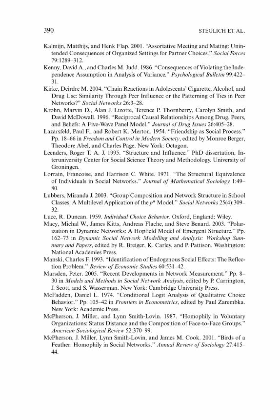
390 STEGLICH ET AL.
Kalmijn, Matthijs, and Henk Flap. 2001. “Assortative Meeting and Mating: Unin-tended Consequences of Organized Settings for Partner Choices.” Social Forces79:1289–312.
Kenny, David A., and Charles M. Judd. 1986. “Consequences of Violating the Inde-pendence Assumption in Analysis of Variance.” Psychological Bulletin 99:422–31.
Kirke, Deirdre M. 2004. “Chain Reactions in Adolescents’ Cigarette, Alcohol, andDrug Use: Similarity Through Peer Influence or the Patterning of Ties in PeerNetworks?” Social Networks 26:3–28.
Krohn, Marvin D., Alan J. Lizotte, Terence P. Thornberry, Carolyn Smith, andDavid McDowall. 1996. “Reciprocal Causal Relationships Among Drug, Peers,and Beliefs: A Five-Wave Panel Model.” Journal of Drug Issues 26:405–28.
Lazarsfeld, Paul F., and Robert K. Merton. 1954. “Friendship as Social Process.”Pp. 18–66 in Freedom and Control in Modern Society, edited by Monroe Berger,Theodore Abel, and Charles Page. New York: Octagon.
Leenders, Roger T. A. J. 1995. “Structure and Influence.” PhD dissertation, In-teruniversity Center for Social Science Theory and Methodology. University ofGroningen.
Lorrain, Francoise, and Harrison C. White. 1971. “The Structural Equivalenceof Individuals in Social Networks.” Journal of Mathematical Sociology 1:49–80.
Lubbers, Miranda J. 2003. “Group Composition and Network Structure in SchoolClasses: A Multilevel Application of the p* Model.” Social Networks 25(4):309–32.
Luce, R. Duncan. 1959. Individual Choice Behavior. Oxford, England: Wiley.Macy, Michal W., James Kitts, Andreas Flache, and Steve Benard. 2003. “Polar-
ization in Dynamic Networks: A Hopfield Model of Emergent Structure.” Pp.162–73 in Dynamic Social Network Modelling and Analysis: Workshop Sum-mary and Papers, edited by R. Breiger, K. Carley, and P. Pattison. Washington:National Academies Press.
Manski, Charles F. 1993. “Identification of Endogenous Social Effects: The Reflec-tion Problem.” Review of Economic Studies 60:531–42.
Marsden, Peter. 2005. “Recent Developments in Network Measurement.” Pp. 8–30 in Models and Methods in Social Network Analysis, edited by P. Carrington,J. Scott, and S. Wasserman. New York: Cambridge University Press.
McFadden, Daniel L. 1974. “Conditional Logit Analysis of Qualitative ChoiceBehavior.” Pp. 105–42 in Frontiers in Econometrics, edited by Paul Zarembka.New York: Academic Press.
McPherson, J. Miller, and Lynn Smith-Lovin. 1987. “Homophily in VoluntaryOrganizations: Status Distance and the Composition of Face-to-Face Groups.”American Sociological Review 52:370–99.
McPherson, J. Miller, Lynn Smith-Lovin, and James M. Cook. 2001. “Birds of aFeather: Homophily in Social Networks.” Annual Review of Sociology 27:415–44.
SEPARATING SELECTION FROM INFLUENCE 391
Mizruchi, Mark S. 1993. “Cohesion, Equivalence, and Similarity of Behavior: ATheoretical and Empirical Assessment.” Social Networks 15:275–307.
Moffitt, Robert A. 2001. “Policy Interventions, Low-Level Equilibria, and SocialInteractions.” Pp. 45–82 in Social Dynamics, edited by Steven N. Durlauf andH. Peyton Young. Cambridge, MA: MIT Press.
Moody, James. 2002. “Race, School Integration, and Friendship Segregation inAmerica.” American Journal of Sociology 107:679–716.
Moran, Patrick A. P. 1948. “The Interpretation of Statistical Maps.” Journal of theRoyal Statistical Society, Series B, 10:245–51.
Mouw, Ted. 2006. “Estimating the Causal Effect of Social Capital: A Review ofRecent Research.” Annual Review of Sociology 32:79–102.
Napier, Ted L., W. Richard Goe, and Douglas C. Bachtel. 1984. “An Assessmentof the Influence of Peer Association and Identification on Drug Use AmongRural High School Students.” Journal of Drug Education 14:227–48.
Newcomb, Theodore M. 1962. “Student Peer-Group Influence.” Pp. 469–88 inThe American College: A Psychological and Social Interpretation of the HigherLearning, edited by Nevitt Sanford. New York: Wiley.
Norris, James R. 1997. Markov Chains. Cambridge, England: Cambridge Univer-sity Press.
Oetting, Eugene R., and Fred Beauvais. 1987. “Peer Cluster Theory, Socializa-tion Characteristics, and Adolescent Drug Use: A Path Analysis.” Journal ofCounseling Psychology 34:205–13.
Oetting, Eugene R., and Joseph F. Donnermeyer. 1998. “Primary SocializationTheory: The Etiology of Drug Use and Deviance. I.” Substance Use and Misuse33:995–1026.
Olson, Mancur. 1965. The Logic of Collective Action: Public Goods and the Theoryof Groups. Cambridge, MA: Harvard University Press.
Padgett, John, and Christopher Ansell. 1993. “Robust Action and the Rise of theMedici, 1400–1434.” American Journal of Sociology 98(6):1259–319.
Pattison, Philippa E., and Garry L. Robins. 2002. “Neighbourhood-based Modelsfor Social Networks.” Pp. 301–37 in Sociological Methodology, vol. 32, editedby Ross M. Stolzenberg. Boston, MA: Blackwell Publishing.
Pearson, Michael, and Lynn Michell. 2000. “Smoke Rings: Social Network Anal-ysis of Friendship Groups, Smoking, and Drug-Taking.” Drugs: Education,Prevention and Policy 7(1):21–37.
Pearson, Michael, and Patrick West. 2003. “Drifting Smoke Rings: Social NetworkAnalysis and Markov Processes in a Longitudinal Study of Friendship Groupsand Risk-Taking.” Connections 25(2):59–76.
Pearson, Michael, Christian Steglich, and Tom A. B. Snijders. 2006. “Homophilyand Assimilation Among Sport-Active Adolescent Substance Users.” Connec-tions 27(1):51–67.
Powell, Walter W., Douglas R. White, Kenneth W. Koput, and Jason Owen-Smith.2005. “Network Dynamics, and Field Evolution: The Growth of Interorga-nizational Collaboration in the Life Sciences.” American Journal of Sociology110:1132–205.
392 STEGLICH ET AL.
Pudney, Stephen. 1989. Modelling Individual Choice. Oxford, England: Basil Black-well.
Richards, William D. 1995. NEGOPY 4.30 Manual and User’s Guide. Burnaby,British Columbia: School of Communication, Simon Fraser University.
Robins, Garry, Peter Elliott, and Philippa Pattison. 2001. “Network Models forSocial Selection Processes.” Social Networks 23:1–30.
Robins, Garry, and Philippa Pattison. 2005. “Interdependencies and Social Pro-cesses: Dependence Graphs and Generalized Dependence Structures.” Pp. 192–214 in Models and Methods in Social Network Analysis, edited by P. Carrington,J. Scott, and S. Wasserman. New York: Cambridge University Press.
Robins, Garry, Philippa Pattison, and Peter Elliott. 2001. “Network Models forSocial Influence Processes.” Psychometrika 6:161–90.
Schweinberger, Michael. 2004. “Statistical Modeling of Network Panel Data:Goodness-of-Fit.” Unpublished Manuscript.
Simons-Morton, Bruce, and Rusan S. Chen. 2005. “Over Time Relationships Be-tween Early Adolescent and Peer Substance Use.” Addictive Behaviors 31:1211–23.
Singer, Hermann. 1998. “Continuous Panel Models with Time Dependent Param-eters.” Journal of Mathematical Sociology 23:77–98.
Snijders, Tom A. B. 2001. “The Statistical Evaluation of Social Network Dynam-ics.” Pp. 361–95 in Sociological Methodology, vol. 31, edited by M. E. Sobel andM. P. Becker. Boston, MA: Blackwell Publishing.
——. 2005. “Models for Longitudinal Network Data.” Pp. 215–47 in Models andMethods in Social Network Analysis, edited by P. Carrington, J. Scott, and S.Wasserman. New York: Cambridge University Press.
Snijders, Tom A. B., and Chris Baerveldt. 2003. “A Multilevel Network Studyof the Effects of Delinquent Behavior on Friendship Evolution.” Journal ofMathematical Sociology 27:123–51.
Snijders, Tom A. B., Christian Steglich, and Michael Schweinberger. 2007. “Mod-eling the Coevolution of Networks and Behavior.” Pp. 41–71 in LongitudinalModels in the Behavioral and Related Sciences, edited by K. van Montfort, H.Oud, and A. Satorra. Mahwah, NJ: Lawrence Erlbaum.
Sprenger, Karel J. A., and Frans N. Stokman. 1995. GRADAP: Graph Definition andAnalysis Package. Groningen: ProGamma.
Steglich, Christian, Tom A. B. Snijders, and Patrick West. 2006. “Applying SIENA:An Illustrative Analysis of the Coevolution of Adolescents’ Friendship Net-works, Taste in Music, and Alcohol Consumption.” Methodology 2:48–56.
Stokman, Frans N., and Patrick Doreian. 1997. “Evolution of Social Networks:Processes and Principles.” Pp. 233–50 in Evolution of Social Networks, edited byPatrick Doreian and Frans N. Stokman. Amsterdam: Gordon and Breach.
Taylor, Shelley E., and Jennifer Crocker. 1981. “Schematic Biases of Social Infor-mation Processing.” Pp. 89–134 in Social Cognition: The Ontario Symposium,vol. 1, edited by E. Tory Higgins, C. Peter Herman, and Mark P. Zanna. Hills-dale, NJ: Erlbaum.
SEPARATING SELECTION FROM INFLUENCE 393
Thornberry, Terence P., and Marvin D. Krohn. 1997. “Peers, Drug Use, and Delin-quency.” Pp. 218–33 in Handbook of Antisocial Behavior, edited by D. M. Stoff,J. Breiling, and J. D. Maser. New York: Wiley.
Valente, Thomas W. 2003. “Social Network Influences on Adolescent SubstanceUse: An Introduction.” Connections 25(2):11–16.
van de Bunt, Gerhard G., Marijtje A. J. van Duijn, and Tom A. B. Snijders. 1999.“Friendship Networks Through Time: An Actor-Oriented Dynamic Statisti-cal Network Model.” Computational and Mathematical Organization Theory5(2):167–92.
Wasserman, Stanley, and Katherine Faust. 1994. Social Network Analysis: Methodsand Applications. New York: Cambridge University Press.
[Note: Corrections were added to the article on 1 October 2010 af-ter first publication online on 15 June 2010. The second part ofequation (6) was incorrect and has been amended in this version, equa-tion (7) has been amended to be in line with the corrections made toequation (6).]


