1
Does Education Really Disadvantage Women
in the Marriage Market?
Elaina Rose* Department of Economics, #353330
University of Washington Seattle, WA 98195
Working Paper No. 33
Center for Statistics and the Social Sciences
University of Washington
July 2003
* This research was supported by NIH Grant R03HD41611. I am grateful to Janet Currie, Henry Farber, Shoshana Grossbard-Schechtman and Levis Kochin for helpful comments and suggestions. Kisa Watanabe provided excellent research assistance.
2
Abstract
The last several decades have seen profound changes in the roles of women in the labor market and the family, with both the media and academic research emphasizing the conflict that women face between their roles in the two spheres. One recurring theme is the “success penalty”, or the disadvantage career success poses to women in the marriage market. In this paper I use data from the U.S. Census to track this success penalty in terms of the relationship between education and marriage for women age 40-44 over the period 1980 through 2000. In 1980, the relationship between education and marriage was essentially an inverted “U”, peaking at 12-16 years of education. When measured as the difference between the likelihood of marriage at the peak of the “U” and the likelihood at the highest level of education, the penalty fell substantially in both the 1980’s and 1990’s. In each year, there are “sheepskin effects” which appear as peaks in the “Currently Married” profiles at high school and college completion, but there are no comparable sheepskin effects in the “Ever Married” profiles. The relationship between education and marriage is also studied for men, by race, and allowing for cohabiting in the definition of marriage. I also track the relationship between education and motherhood; the tradeoff between these two outcomes appears to be declining as well. The decline in the disadvantaged faced by educated women in terms of family outcomes suggests that specialization and exchange is playing less of a role in marriage, and/or that the social norm for hypergamy (i.e., women “marrying up”) has shifted.
3
I. Introduction
The last several decades have seen profound changes in the roles of women in the labor market
and the family. One subject of concern has been the conflict that women face between their roles in the
two spheres. Several writers have noted that the ideal of “having it all” proved elusive for American
women in the late 20th century. For instance, Goldin (1997) demonstrates the paucity of women
college graduates from the breakthrough generation (graduating between 1966 and 1979) who managed
to achieve both family and career success by 1988.
One recurring theme in both the media and in academic research is the “success penalty”, or
the disadvantage career success poses to women in the marriage market. For instance, Sylvia Hewlett
reports: “the rule of thumb seems to be that the more successful the woman, the less likely it is that she
will find a husband or bear a child. For men the reverse is true.” 1 Maureen Dowd followed up on
Hewlett’s work in a series of New York Times columns last year, stating in one: “Men veer away from
‘challenging’ women because they have an atavistic desire to be the superior force in a relationship”2.
Several letters in response to the Times column support the perception that success disadvantages
women’s prospects for marriage.3 Hewlett emphasizes that one consequence of the success penalty is
the limited opportunities for career women to bear and raise children.
What is the source of the penalty? Historically, and in a variety of settings, there is a social
norm for what anthropologists call “female hypergamy”, that is, women tending to marry up on various
dimensions. For instance, Miller [1981] reports that in some parts of India strong pressures for
hypergamy imply a lack of suitable husbands for high caste girls, resulting in female infanticide. In
another context, the Talmud advises men to “go down a step to take a wife,” (Yevamot, 63a) because,
according to Rashi, “a woman from a more distinguished family than her husband may consider
herself superior and act haughtily toward him”.4
1 Dowd [2002]. 2 Dowd [2002]. 3 Although one man (Naidich [2002]) did respond with skepticism. 4 I am grateful to Levis Kochin and David Twersky for these references.
4
Hypergamy can be the result of a model of specialization and exchange as well as social norms.
As Becker [1974] shows, the returns from specialization and exchange are greater when partners differ
in market relative to home productivity. In the traditional model, men specialize in the market and
women specialize in the home. If education increase market productivity more than home productivity,
then marital surplus will be greater in hypergamous marriages. Regardless of whether it is the outcome
of a model of specialization and exchange or the result of social norms, hypergamy with respect to
education can lead to a success penalty as it tends to disadvantage women at the top of the distribution.
The first objective of this paper is to estimate the success penalty in terms of the relationship
between education and marriage market outcomes, for women in their early 40’s. The focus is on
education, rather than, say, income, in that the former is less apt to be endogenous with respect to
marriage and parenthood.
The second objective is to test for a shift in the relationship between education and marriage in
the latter decades of the 20th century. The direction of a shift is ambiguous a priori. On one hand,
there is an “excess supply effect”: Women’s education has increased substantially in the last several
decades, both in absolute terms and relative to men. Hypergamy, combined with an increased supply
of women with college and advanced degrees would tend to increase the competition of successful
women for appropriate partners, and exacerbate the success penalty.
On the other hand, the nature of marriage has changed as well. The conventional “Leave it to
Beaver” marriage of the 1950’s and 60’s in which the husband worked in the labor market and the wife
took care of the home has given way to a new norm in which both spouses work.5 Both a shift in social
norms and a decline in the returns to specialization in marriage would lead to a “decline in hypergamy”
effect. This decline in hypergamy resulting from a decline in the returns to specialization would be
similar to Lam’s [1988] result that a decline in the returns to specialization6 would lead to more
5 Jacobson [1998] reports changes in labor force participation rates for married women. Blau [1998] reports that women in 1988 spent significantly less, and men spend somewhat more, time on housework than in 1978. 6Evidence of a decline in the role of specialization within marriage includes Lundberg and Rose [1999]
5
positive assortative mating – i.e., an increase in the degree of similarity of spouses7 reduce the
disadvantage faced by successful women in the marriage market.8
In this paper, I use data from the U.S. Census of Population for 1980, 1990 and 2000 to track
the relationship between education and two marriage outcomes – “Currently Married” and “Ever
Married” –for women age 40-44. In 1980, the relationships were highly non-linear: an inverted-U
shapes peaking at between 12 and 16 years of education. In terms of the outcome “Currently Married”,
the data show what appear to be “sheepskin effects” in marriage outcomes: spikes in the
education/marriage profile at 12- and 16- years of education. While the profiles shifted down in each
of the two subsequent decades, the negative relationship between education and marriage at the higher
end of the distribution weakened substantially. When measured as the difference in the likelihood of
being currently married with a graduate/professional degree relative to a bachelors degree, the success
penalty fell significantly and substantially over the period – from 15.7 in 1980 to 1.6 percentage points
in 2000. The penalty measured in terms of “Ever Married fell from 11.1 percentage points to 2.6
percentage points.
The third objective of the paper is to explore reasons for the discrepancy between the popular
perceptions as well as research pointing to a substantial success penalty, and the finding here that the
success penalty is minimal. I estimate the relationship between education and marriage for men,
examine differences by race, address the role of cohabitation, and track the relationship between
education and motherhood as well as marriage. In short, as cohabitation is relatively rare for
individuals age 40-44, it does not explain the changing relationship between education and marriage.
There is little evidence of the existence of a success penalty at all for black women over the period.
Finally, the tradeoff between education and motherhood appears to be declining, as well. and Gray [1997]. 7 In fact, Mare [1999] finds less assortative mating on education in the period 1940-1980. Using data from the Panel Study of Income Dynamics (PSID), Rose [2001] finds evidence of a decline in assortative mating and hypergamy with respect to college completion, and parent’s education between 1970 and 1990. 8 Goldstein and Kenney report that women with college education are more relatively more likely to be married in 1980 than in 1960.
6
Section II of this paper discusses the data used for the analysis. Section III presents graphs of
the relationship between education and marriage as well as probit regression results. Section IV
concludes.
II. Data
The data are from the United States Census of Population Public Use Microdata Sample
(PUMS). For 1980 and 1990, I used the 5% Public Use Microdata Sample (PUMS), and for 2000 I
used the 1% sample. For most of the analyses, the outcome is “marriage”. Two measures of marital
status are used: whether the individual is currently married (“Currently Married” or “Current” for
short), and whether the individual has ever been married (“Ever Married”, or “Ever”). “Current” is a
dummy variable which equals one if the individual is currently married – whether living with spouse or
separated. “Ever” equals one if “Current” equals one or if the individual is a widow or is divorced.
Because cohabitation has become a partial substitute for marriage over the period (Bumpass et
al, 1991), I also look at the outcome “Cohabiting” – whether an individual is currently married or
cohabiting. Cohabiting was defined as adjusted Persons of Opposite Sex Sharing Living Quarters
(POSSLQ), following the definitions set out in Casper et al [1999] for 1980, and was identified as
“unmarried partner” in 1990 and 2000.
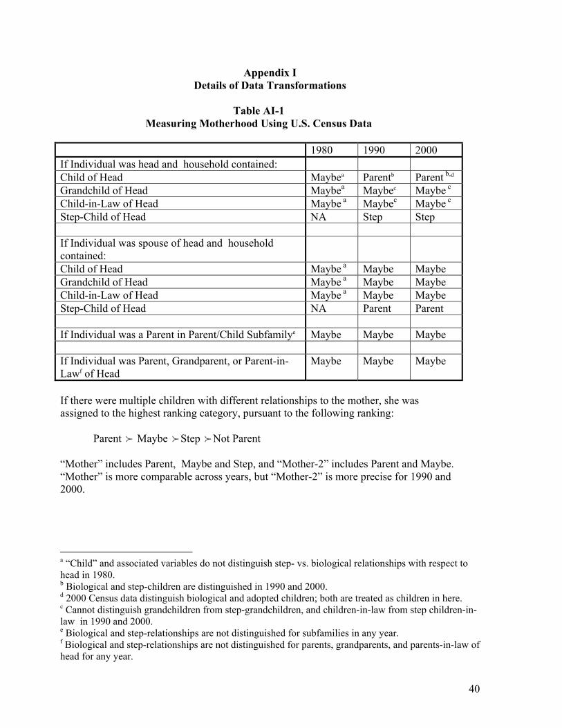
For some analyses, the outcome is motherhood (“Mother”). Unfortunately, only an imperfect
measure of motherhood is available from the Census. As the Census only asks about individuals
residing within a household, parents of children residing elsewhere may be misclassified. Another
problem is that in 1980, and in later years for some individuals living in sub-families, it is not possible
to distinguish co-resident step-children from biological children. Appendix Table A-1 details
the method used to develop the measure of motherhood. When women could be definitively identified
as biological or adoptive mothers, they are classified as “Parent”. When they are determined to be
step-mothers, but not biological or adoptive mothers, they are classified as “Step”. When it is not clear
7
if they are biological adoptive mothers or step-mothers, they are classified as “Maybe”. I use a
definition that includes “Maybe” and “Step” in the definition of motherhood, as it is consistent over the
three surveys. An alternative measure, “Mother-2”, does not include “Step”. While this measure is
more precise in 1990 and 2000, it is not consistent with the best definition available for 1980.
Another complication is that the coding of education changed between 1980 and 1990. In
1980, each respondent reported the number of years of school attended and whether the final year was
completed. The questions in 1990 and 2000 focused more on degrees attained. The 1980 measures
were collapsed to aggregate the small cell counts at low levels of education to obtain the variable “Edu-
1”. “Edu-1” was collapsed further to “Edu-2” which is comparable to the 1990 and 2000 measures.
The correspondence between the education measures is outlined in Appendix Table A-2..
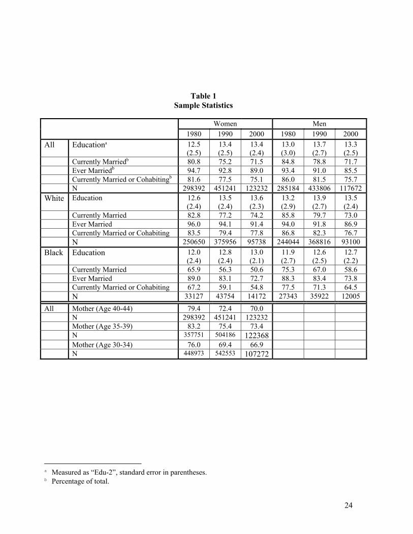
Table 1 reports characteristics of the sample in each year for men and women, and for whites
and blacks separately. Women’s education increased more than men’s over the period. On average,
women age 40-44 had 12.5 years of education in 1980, which increased to 13.4 in 2000. The
comparable numbers for men are 13.0 and 13.3.
While there has clearly been a decline in marriage, the vast majority of both men and women
have been married at some time in their lives by age 40-44. Even in 2000, 89.0 percent of all women,
and 85.5 percent of all men had been married at some point. Due to the possibility of divorce (and to a
minor extent, widowhood), fewer individuals report being currently married than having ever been
married. The percentage of women currently married fell from 71.5 percent in 1980 to 89.0 percent in
2000; the comparable numbers for men are 84.8 and 71.7 percent, respectively.
The second panel reports the same statistics for whites. As whites dominate the sample, it is
not surprising that the patterns for whites are similar to those for the sample as a whole, with marriage
rates and education being somewhat higher.
The bottom panel reports the same statistics for blacks. Education has increased more
markedly for black men relative to white men over the period, but the increase for black women is
similar to that of white women. Marriage rates for blacks, however, are substantially lower than those
8
for whites, and their decline over the period has been more precipitous. For instance, in 1980, 65.9
percent of black women in the sample were currently married, the percentage fell by 15.3 points, to
50.6 percent by 2000.9
While cohabitation overall has increased, it is still relatively uncommon among individuals in
their early 40’s. For instance, in 2000, only 3.6 of women in the sample were cohabiting, while 71.5
percent were married.
Motherhood appears to have declined as well. In 1980, 79.4 percent of women age 40-44 had
a co-resident child, but the percentage fell to 70.0 percent by 2000. As women in this age group may
have had children in their teens or early twenties that are no longer co-resident, I look at the same
relationships for women age 35-49 and 30-34. The percentage of these women who were mothers fell
by about 10 percentage points for each age category over the twenty-year period.
III. Findings
III.A. Women, Education and Marriage
Linear Specification
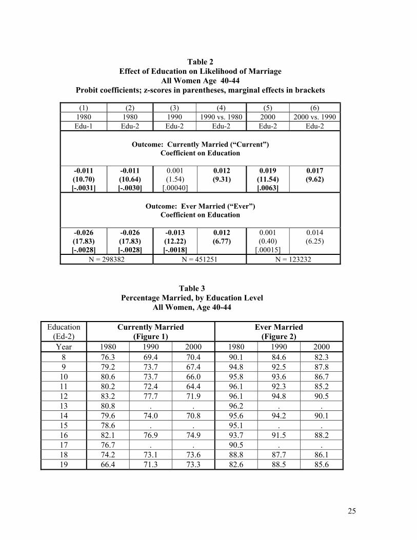
Table 2 reports the probit regression coefficients, t-statistics, and marginal effects with respect
to education on the two marriage outcomes. The top panel refers to refers to “Current”, and the
bottom panel refers to “Ever”. The coefficients in columns (1) and (2) are based on single year
regressions for 1980. Column (1) uses “Edu-1” and Column (2) uses “Edu-2”. Columns (3) and (5)
report coefficients from the single year regressions for 1990 and 2000 respectively, using “Edu-2”.
Columns (4) and (6) are computed from pooled regressions in which the coefficients and intercepts are
allowed to vary by year, and “Edu-2” is used for all years. Column (4) reports the differences in the
education coefficients between 1980 and 1990, and the t-statistics associated with the hypothesis tests
9 The remainder of the sample consists of individuals classified as Asian or “Other”. As this is a heterogeneous group, I didn’t do any analyses with respect to it.
9
that the differences equal zero. The comparable statistics for the differences between the 1990 and
2000 coefficients are reported in Column (6)
In 1980, the effect of education on both “Current” and “Ever” is negative and highly
significant. The coefficients correspond to marginal effects of -.0031 and -.0028, respectively,
indicating that each additional year of education is associated with about a 3.1 percentage point lower
likelihood of being currently married at, and a 2.8 percentage point lower likelihood of having been
married by, age 40-44 in 1980. The two measures of education produce virtually identical results.
In 1990, the coefficient of education on “Current” is not significantly different from zero,
while the comparable coefficient on “Ever” is still negative and significant. In both cases, the
coefficients are significantly smaller (t=9.31 for “Current”, t=6.77 for “Ever”) than in 1980.
The significantly positive coefficient of education on “Current” in 2000 corresponds to a
marginal effect of .0063, indicating that each additional year of education is associated with a 0.63 a
percentage point increase in the likelihood of being married (t=11.54); this also effect is significantly
different than the effect in 1990 (t=9.62). The effect of education on “Ever” is not significant, but is
significantly greater than the 1990 coefficient (t=6.25).
Overall, these results suggest that a significant success penalty existed in 1980, but fell
significantly in each of the subsequent two decades. The 2000 results suggest the existence of a
success premium for the outcome currently married, and no significant relationship between education
and having ever been married.
Plotting the Education/Marriage Profiles
The results in Table 2 are limited in that they restrict the relationship between education and
marriage to be linear. To evaluate whether this assumption is reasonable, the percentage of women
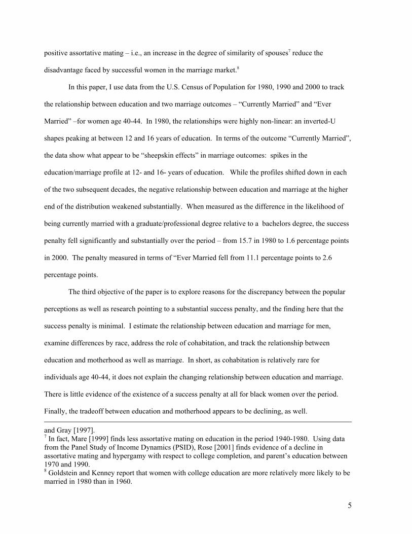
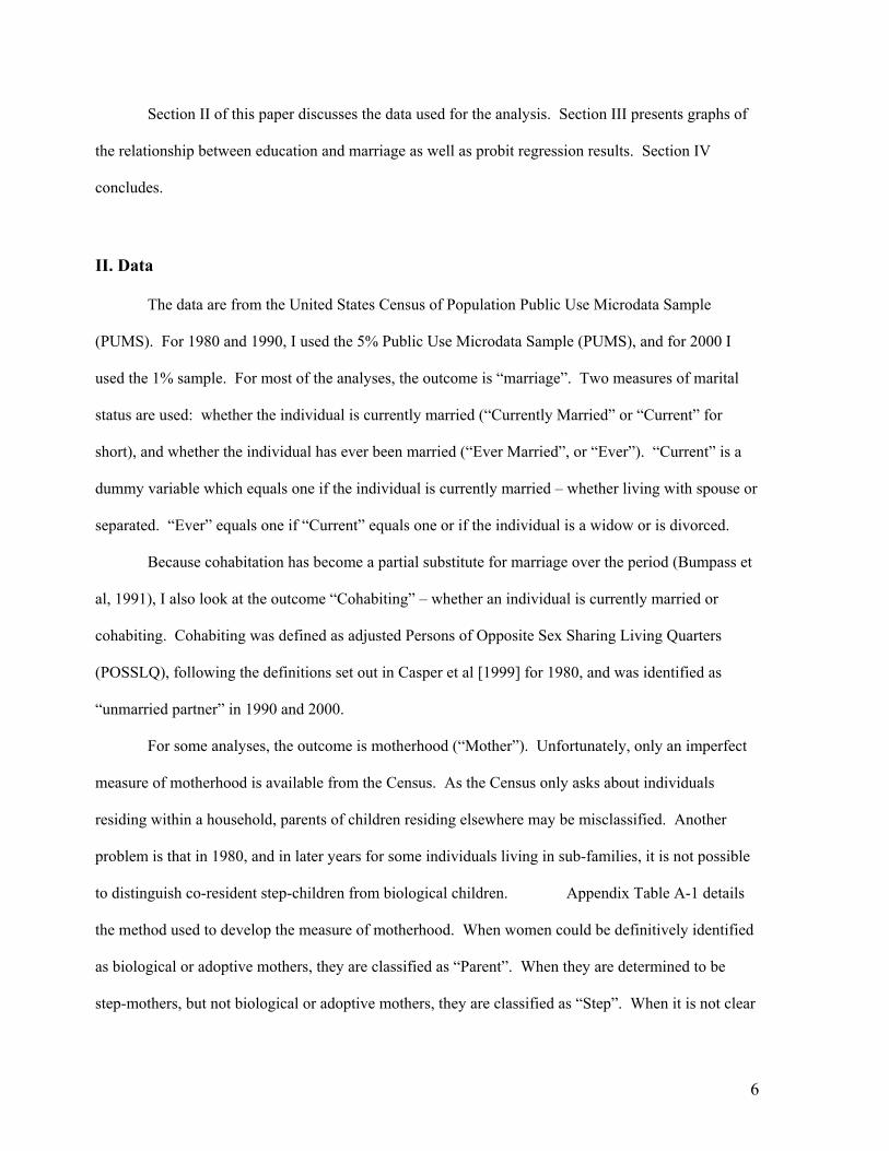
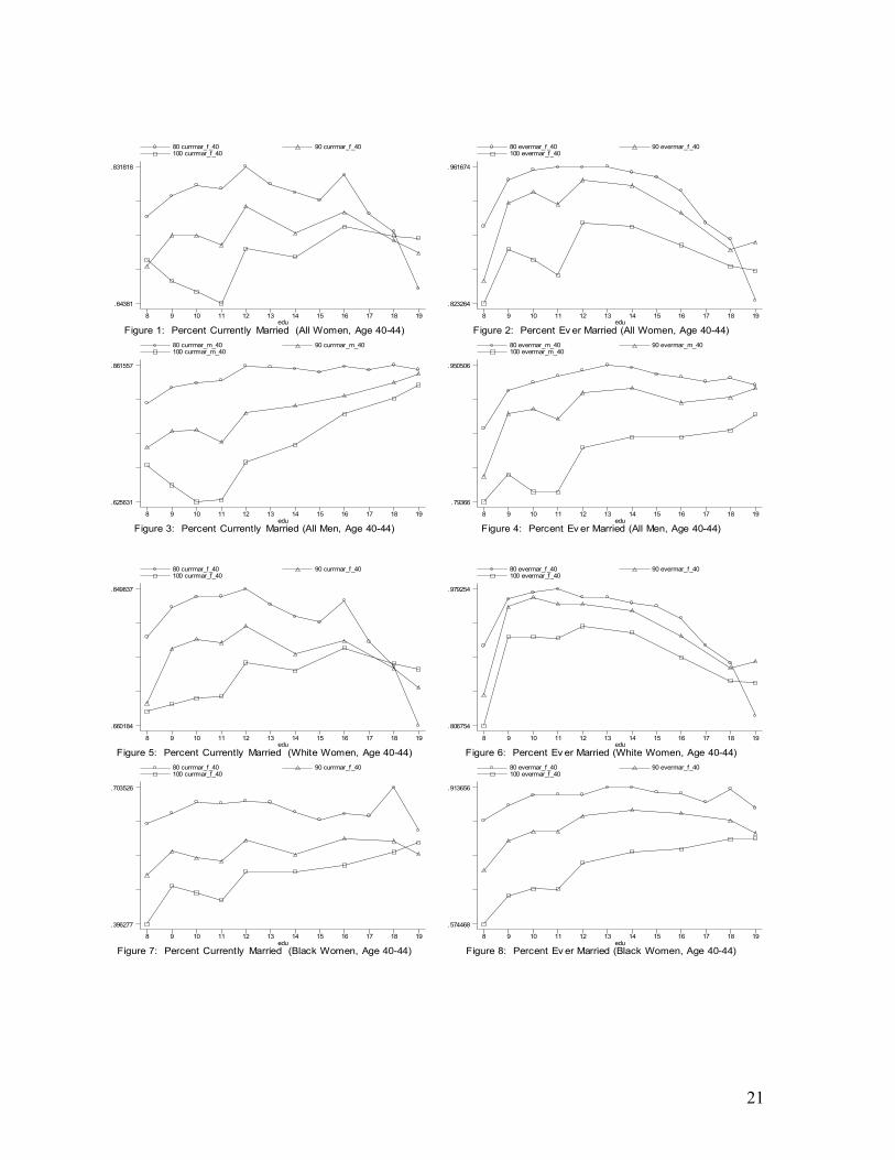
currently and ever married by each level of education are reported in Table 3 and plotted in Figures 1
and 2 for each of the three years. The 1980 data use “Edu-1”, and the 1990 and 2000 data use “Edu-2”.
10
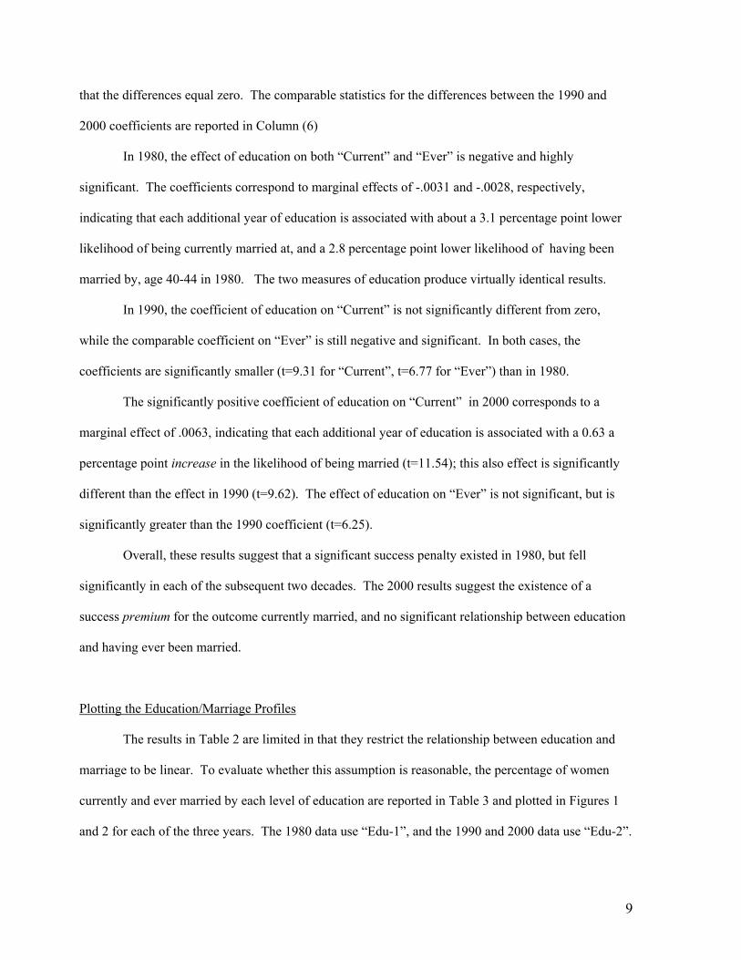
Figure 1 shows that in 1980, the proportion currently married is (weakly) increasing with each
year of education up to twelve years, at which point there is a spike. There is a decline for each of the
following levels of education, and then a spike at sixteen years of education, after which the profile
declines sharply. The profile shifts downward, particularly at lower levels of education, in each of the
two subsequent decades. For 1990, there are still spikes in the profile at twelve and sixteen years of
education; otherwise the profile is flatter. In 2000, other than the two spikes, the profile appears to be
essentially flat or increasing from high school graduation forward.
In 1980, the likelihood of being currently married was substantially lower at 19 years of
education (66.4 percent) relative to the local maximum at year 16 (82.1). The difference of 15.7
percentage points reflects a success penalty consistent with Dowd and Hewlett’s statements. However,
this difference fell in each of the two subsequent decades. By 2000, the difference fell to 1.4
percentage points (73.3 – 71.9 percent). The compression in the profiles at high levels of education
indicates that the widely noted decline in marriage, at least for this age group, has been driven mainly
by women at lower levels of education.
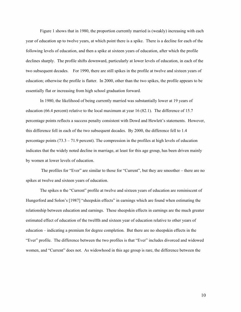
The profiles for “Ever” are similar to those for “Current”, but they are smoother – there are no
spikes at twelve and sixteen years of education.
The spikes n the “Current” profile at twelve and sixteen years of education are reminiscent of
Hungerford and Solon’s [1987] “sheepskin effects” in earnings which are found when estimating the
relationship between education and earnings. These sheepskin effects in earnings are the much greater
estimated effect of education of the twelfth and sixteen year of education relative to other years of
education – indicating a premium for degree completion. But there are no sheepskin effects in the
“Ever” profile. The difference between the two profiles is that “Ever” includes divorced and widowed
women, and “Current” does not. As widowhood in this age group is rare, the difference between the
11
two profiles reflects divorced women and suggests that women who tend to drop out from college are
more likely to “drop out” from marriage.10
Non-Linear Specifications
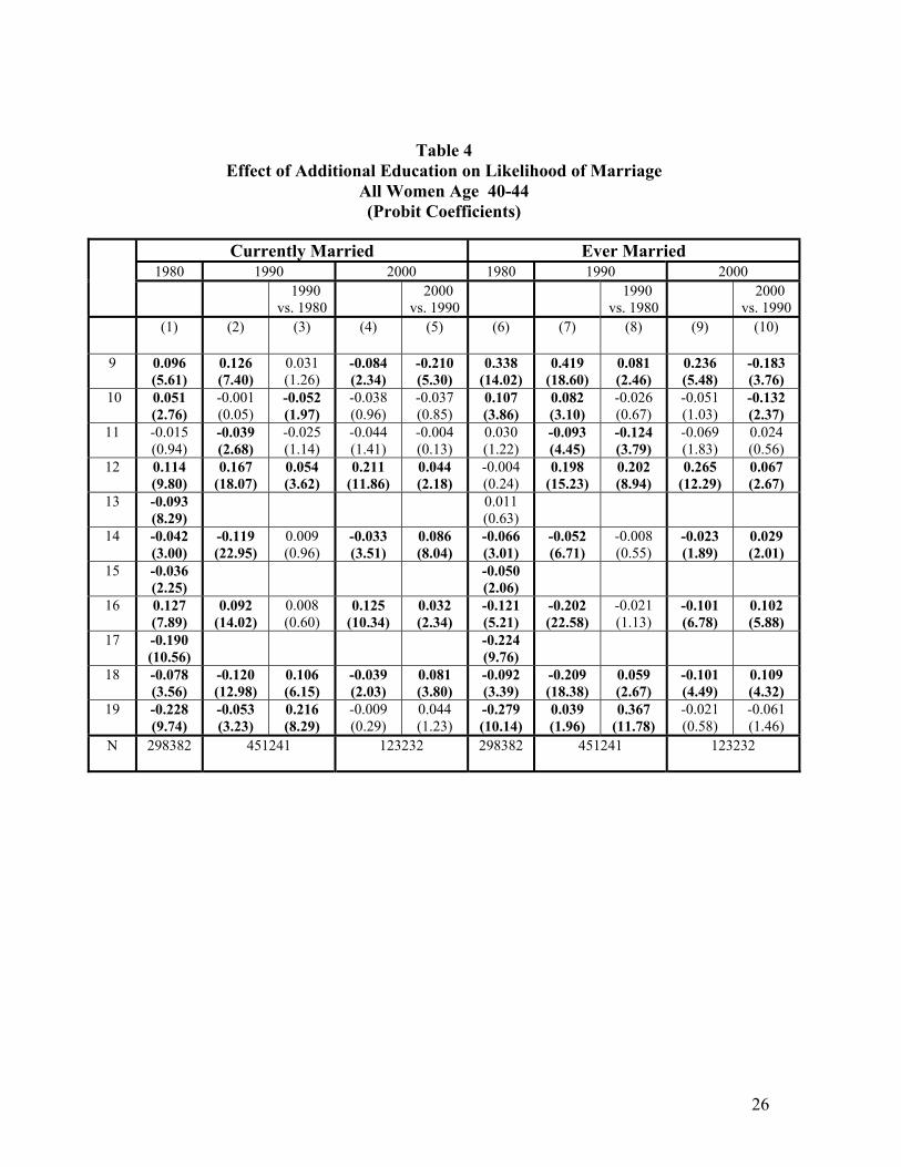
But are these relationships statistically significant? Table 3 presents the results of probit
regression models of the relationship between education and marriage for each of the three years.
Columns (1) through (5) pertain to the outcome “Current” and Columns (6) through (10) pertain to the
outcome “Ever”. Columns (1) and (6) are based on the model for the year 1980 using dummy
variables for each of the levels of “Edu-1”. Columns (2) and (7) are based on the model for the year
1990 using “Edu-2”, and columns (4) and (9) are based on “Edu-2” for 2000. Additionally, pooled
probit regressions were performed for each of the two outcomes (using “Edu-2” for all years) to test
whether the changes in the coefficients between decades were significant. These results are reported in
columns (3) and (5) for “Current” and for columns (8) and (10) for “Ever”.
Education is measured as having at least that level of education, so each coefficient reflects the
incremental effect of that year of education on the continuous latent variable associated with the
outcome being one; the omitted category is eight years of education or less.11 For instance, in 1980,
going from eight to nine years of education increases the latent variable associated with the outcome
that a woman is married by about 9.6 percent, and this change is statistically significant (t=5.61); the
effect of going from nine to ten years is positive and statistically significant (t=2.76), and the effect of
going from ten to eleven years is not statistically significant (t=.94). 10 Another possibility is that women who are divorced are more likely to be attending college at the date of the interview. I examined this using the 1980, which asks whether the individual has completed the respective year of education, or is still attending or dropped out. The percentages currently attending women (men) in the sample were: 3.8 (2.9) percent of married, 4.7 (3.1) percent of widowed, 6.7 (3.3) percent of divorced, 4.9 (3.2) percent of separated and 6.0 (4.1) percent of never married. To the extent that interviews were conducted over the summer, the percentage currently attending do not reflect those still in school but between years in a program. 11 Yes, I know I should report and discuss marginal (or, incremental) effects, and that a significant coefficient does not imply a significant marginal effect. However, the sign of the coefficient and the marginal effect are the same, and the significance levels are not much different. I’ll fix this up in the next version!
12
In 1980, at least throughout high school, education was associated with an increased likelihood
of marriage. The coefficients are positive and significant for the 9th, 10th, and 12th year of education,
and insignificant for the 11th year. However, each year of education between high school and college is
associated with a significantly lower likelihood of marriage, until the “sheepskin” year 16 – typically,
college graduation – when there is a significant increase. Beyond that point, however, each year of
education is associated with a significantly lower likelihood of marriage. So, the “success penalty” is
statistically, as well as quantitatively, significant.
The findings for 1990 reported in Column (2) are qualitatively similar to those for 1980. From
high school graduation forward, the signs of the effects are the same, and all the coefficients are
statistically significant. The standard errors are larger for the 2000 sample, as the sample size is
smaller. Still, from the twelfth year of education forward, the signs are similar to the previous years,
and except for the final transition from masters degree to graduate professional degree, the coefficients
are all statistically significant.
The coefficients in Columns (3) and (5), based on the pooled 1980, 1990 and 2000 data using
Ed-2 for all years, provide the means to test whether the coefficients have changed significantly over
time. In the 1980’s the effect of going from college to master’s degree, and master’s degree to
graduate professional degree fell significantly in absolute value. Overall, the changes in the 1990’s
were significant as well. So, the success penalty declined significantly in each of the two decades.
Moving on to the outcome “Ever” in columns (6) through (10), we find similar results,
although there are no significant sheepskin effects. In 1980, the effect of education on marriage was
negative and significant for each year beyond the thirteenth. In 1990, the effects were negative and
significant for all of these education levels except for the very highest, and the coefficients for the
highest two education levels were significantly smaller in absolute value than in 1980. For 2000, the
effects for the 14th through 18th year were negative, but significantly less so than in 1990.
13
III. B. What About Men?
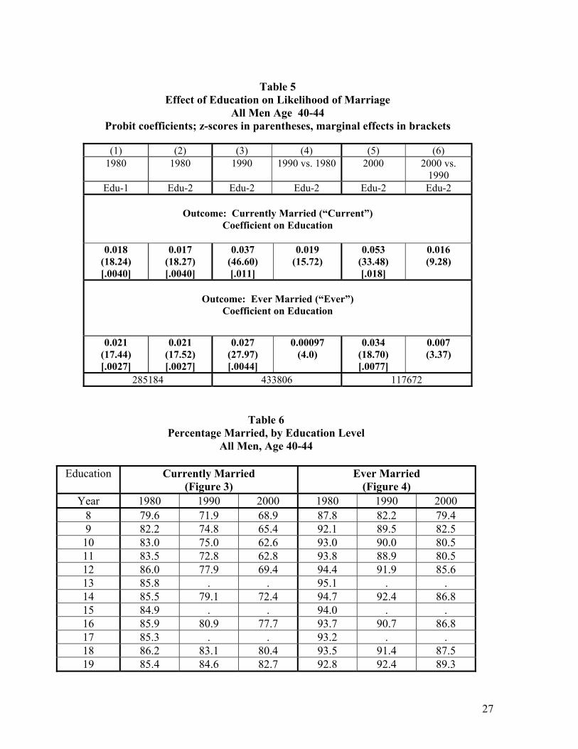
Of course, a complete discussion of the marriage market needs to consider both sides. In this
subsection, I repeat the previous analysis for the comparable sample of men; the results are report in
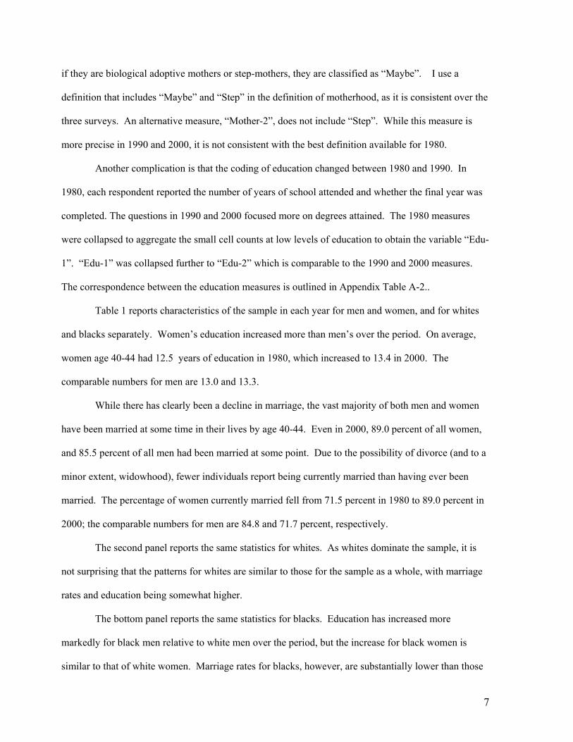
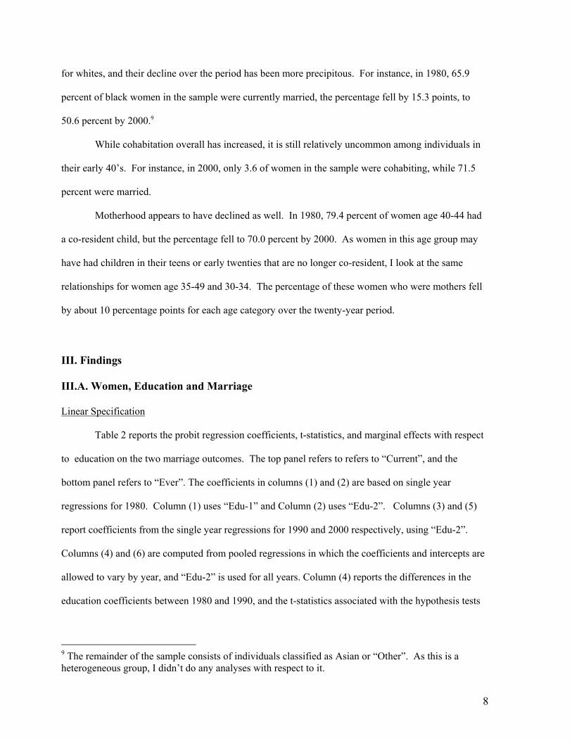
Figures 3 and 4, and Tables 5 through 7.
The results of the linear specification in Table 5 indicate that increased education is associated
with greater likelihood of marriage at all ages. The relationship becomes stronger in each decade. In
1980, an additional year of education results in a 0.4 percentage point increase in the likelihood of
marriage; the comparable numbers for 1990 and 2000 are 1.1 and 1.8 percentage points, respectively.
The increases in the coefficients in each of the two decades are statistically significant (t= 15.72, 9.28
for “Current”, and t= 4.0 and 3.37 for “Ever”, for the 1980’s and 1990’s, respectively).
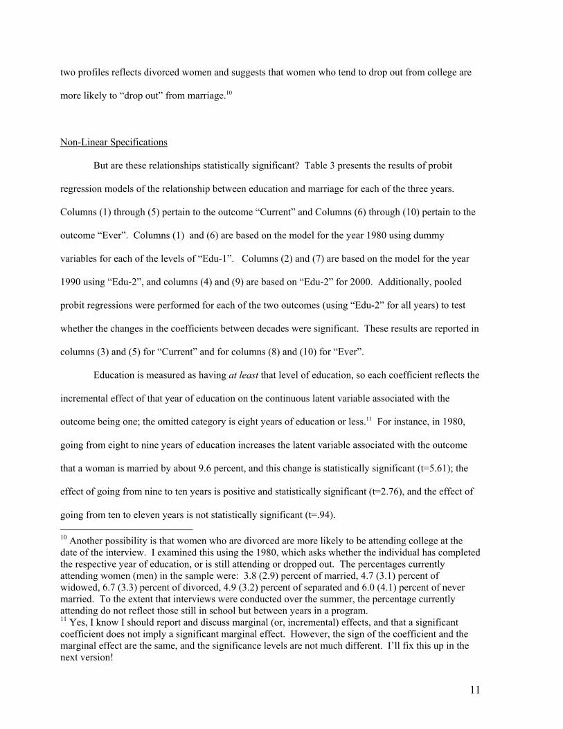
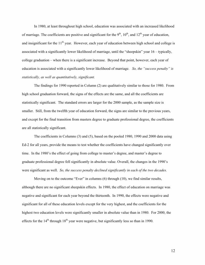
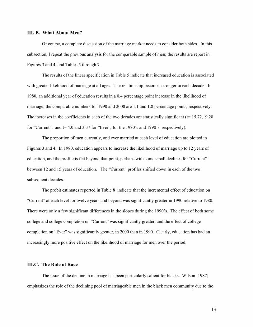
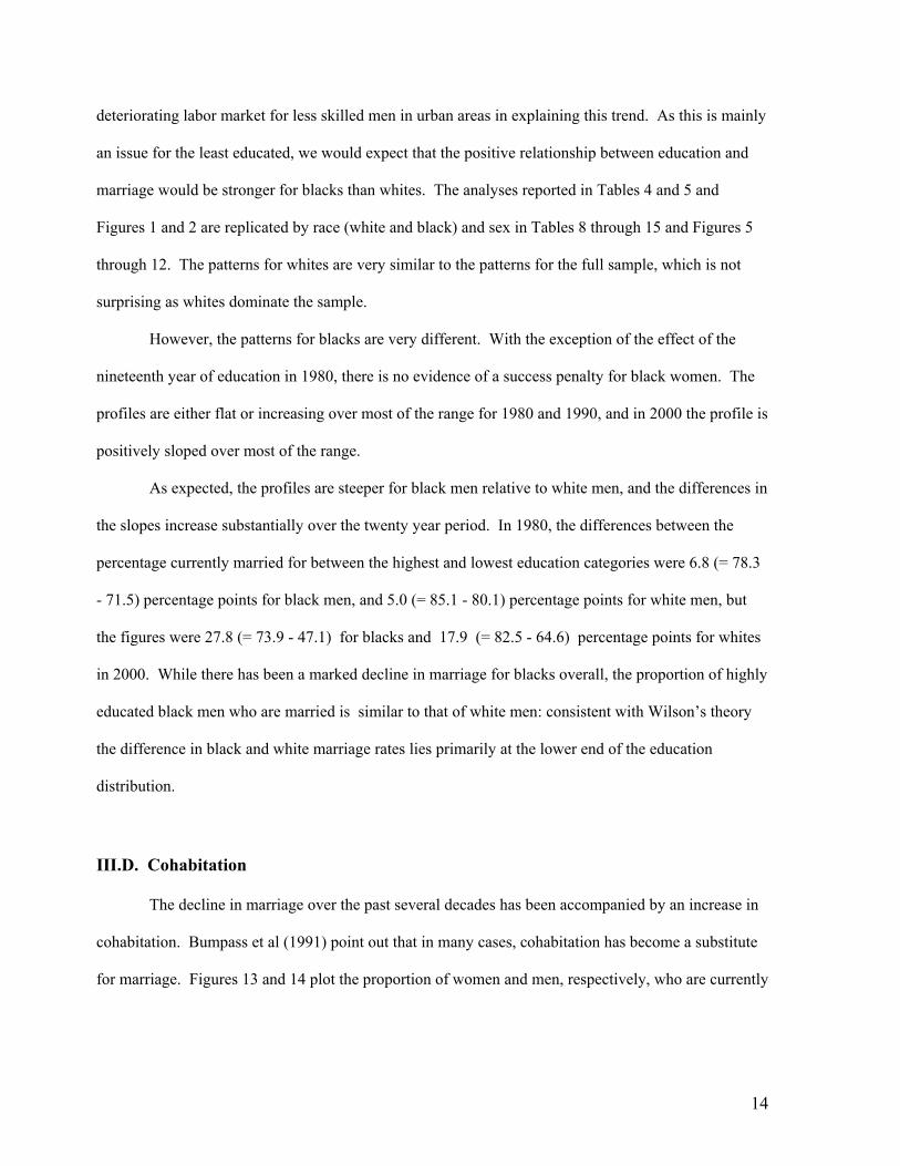
The proportion of men currently, and ever married at each level of education are plotted in
Figures 3 and 4. In 1980, education appears to increase the likelihood of marriage up to 12 years of
education, and the profile is flat beyond that point, perhaps with some small declines for “Current”
between 12 and 15 years of education. The “Current” profiles shifted down in each of the two
subsequent decades.
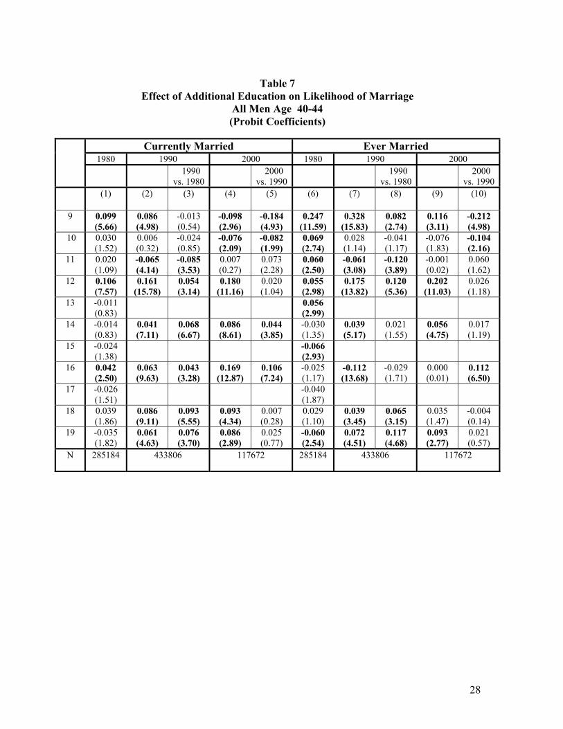
The probit estimates reported in Table 8 indicate that the incremental effect of education on
“Current” at each level for twelve years and beyond was significantly greater in 1990 relative to 1980.
There were only a few significant differences in the slopes during the 1990’s. The effect of both some
college and college completion on “Current” was significantly greater, and the effect of college
completion on “Ever” was significantly greater, in 2000 than in 1990. Clearly, education has had an
increasingly more positive effect on the likelihood of marriage for men over the period.
III.C. The Role of Race
The issue of the decline in marriage has been particularly salient for blacks. Wilson [1987]
emphasizes the role of the declining pool of marriageable men in the black men community due to the
14
deteriorating labor market for less skilled men in urban areas in explaining this trend. As this is mainly
an issue for the least educated, we would expect that the positive relationship between education and
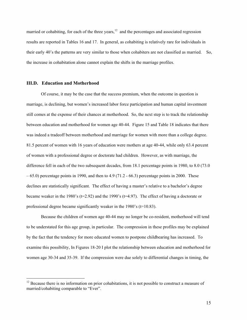
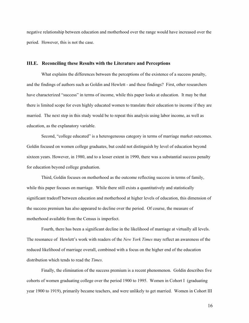
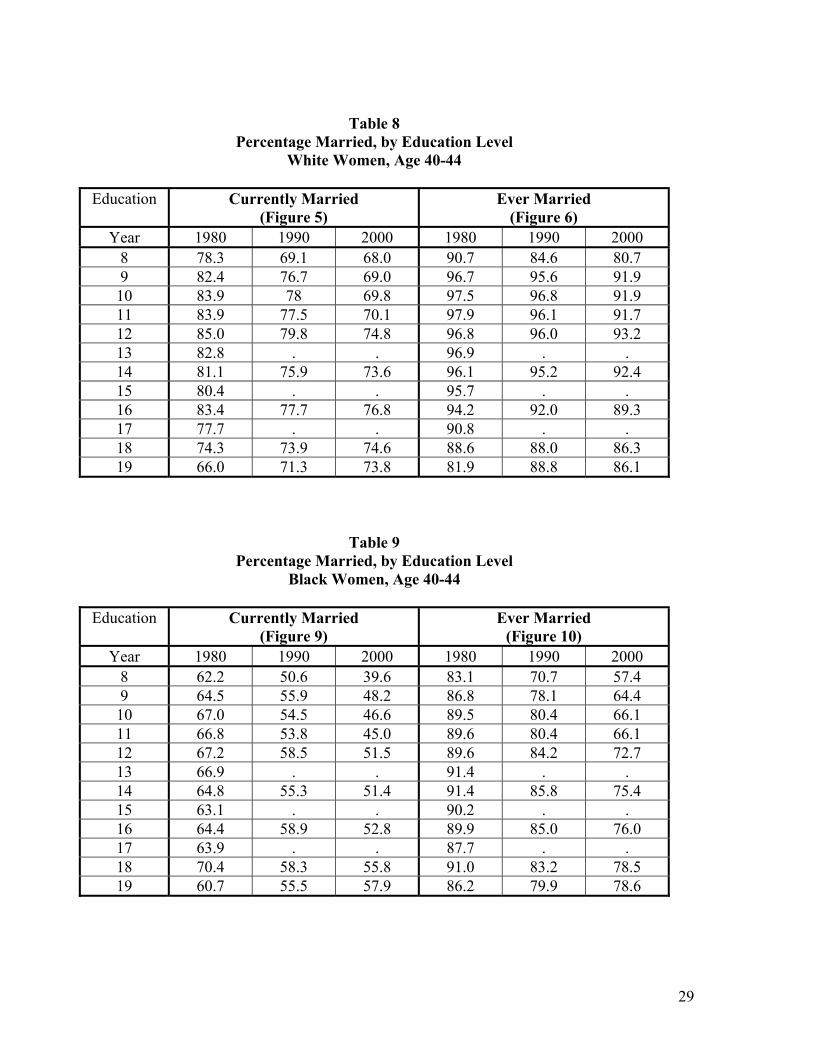
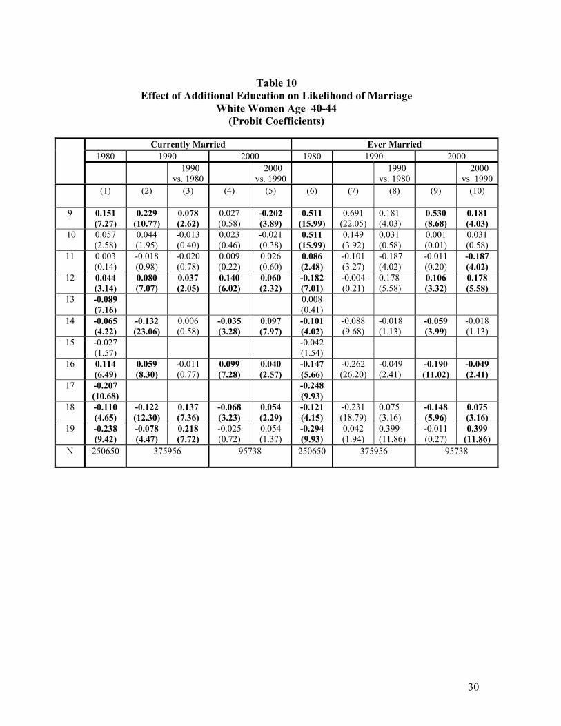
marriage would be stronger for blacks than whites. The analyses reported in Tables 4 and 5 and
Figures 1 and 2 are replicated by race (white and black) and sex in Tables 8 through 15 and Figures 5
through 12. The patterns for whites are very similar to the patterns for the full sample, which is not
surprising as whites dominate the sample.
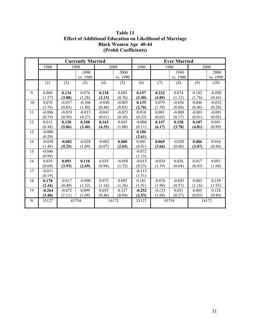
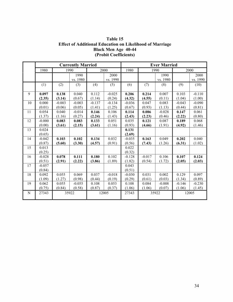
However, the patterns for blacks are very different. With the exception of the effect of the
nineteenth year of education in 1980, there is no evidence of a success penalty for black women. The
profiles are either flat or increasing over most of the range for 1980 and 1990, and in 2000 the profile is
positively sloped over most of the range.
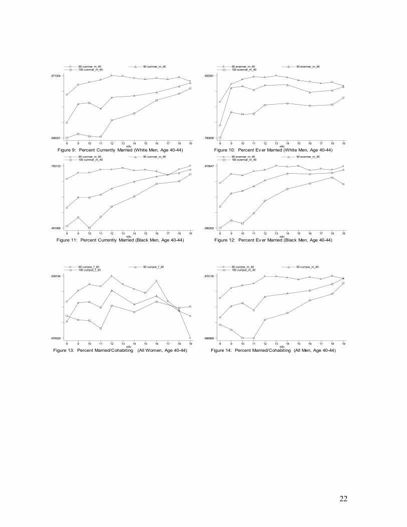
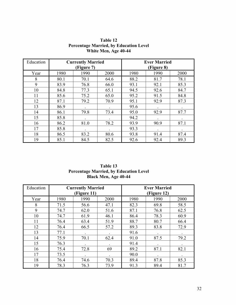
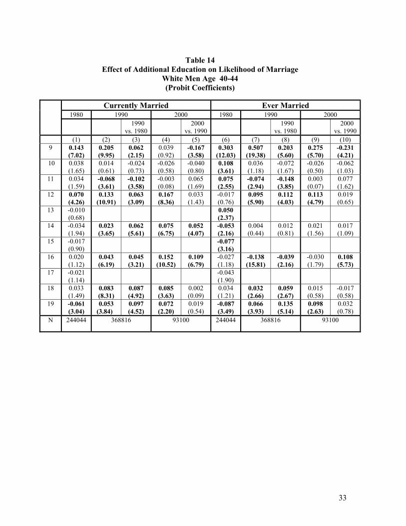
As expected, the profiles are steeper for black men relative to white men, and the differences in
the slopes increase substantially over the twenty year period. In 1980, the differences between the
percentage currently married for between the highest and lowest education categories were 6.8 (= 78.3
- 71.5) percentage points for black men, and 5.0 (= 85.1 - 80.1) percentage points for white men, but
the figures were 27.8 (= 73.9 - 47.1) for blacks and 17.9 (= 82.5 - 64.6) percentage points for whites
in 2000. While there has been a marked decline in marriage for blacks overall, the proportion of highly
educated black men who are married is similar to that of white men: consistent with Wilson’s theory
the difference in black and white marriage rates lies primarily at the lower end of the education
distribution.
III.D. Cohabitation
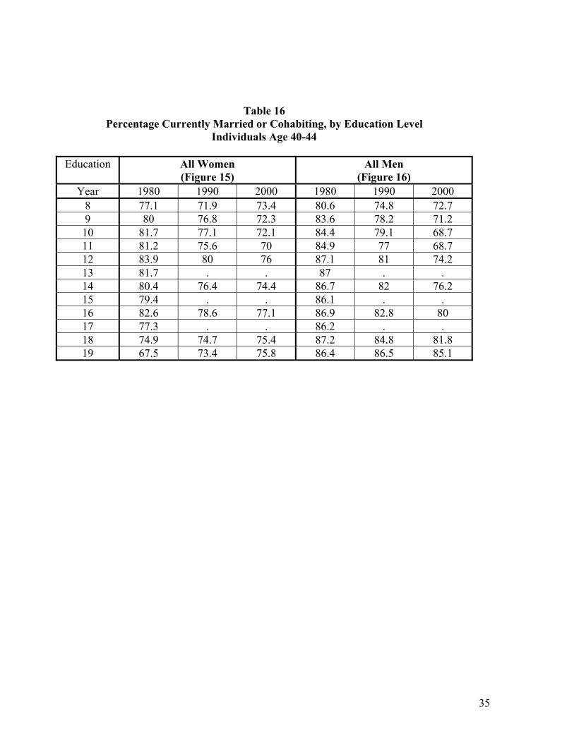
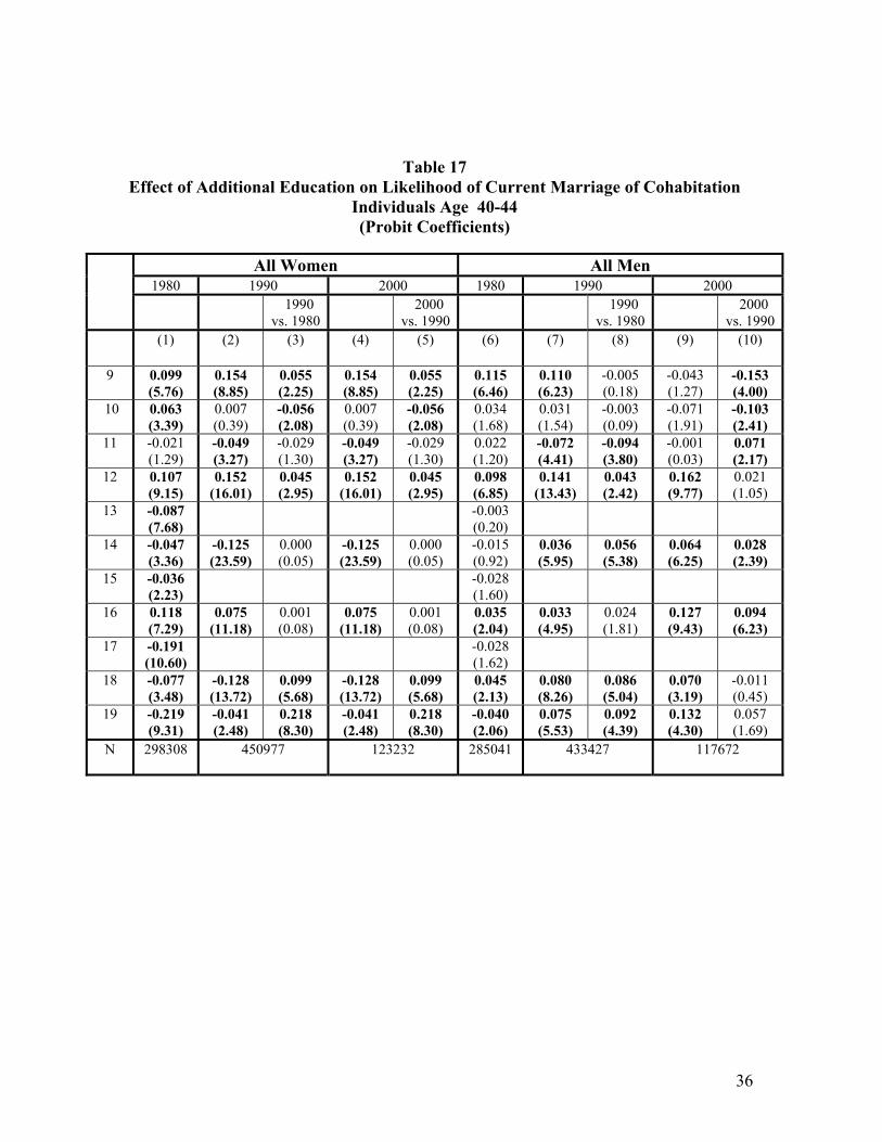
The decline in marriage over the past several decades has been accompanied by an increase in
cohabitation. Bumpass et al (1991) point out that in many cases, cohabitation has become a substitute
for marriage. Figures 13 and 14 plot the proportion of women and men, respectively, who are currently
15
married or cohabiting, for each of the three years,12 and the percentages and associated regression
results are reported in Tables 16 and 17. In general, as cohabiting is relatively rare for individuals in
their early 40’s the patterns are very similar to those when cohabiters are not classified as married. So,
the increase in cohabitation alone cannot explain the shifts in the marriage profiles.
III.D. Education and Motherhood
Of course, it may be the case that the success premium, when the outcome in question is
marriage, is declining, but women’s increased labor force participation and human capital investment
still comes at the expense of their chances at motherhood. So, the next step is to track the relationship
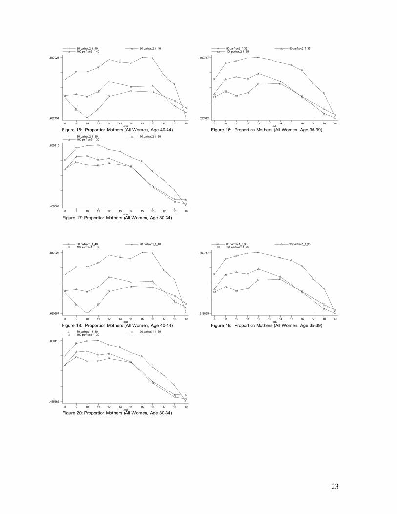
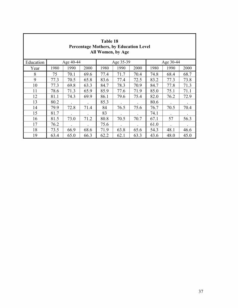
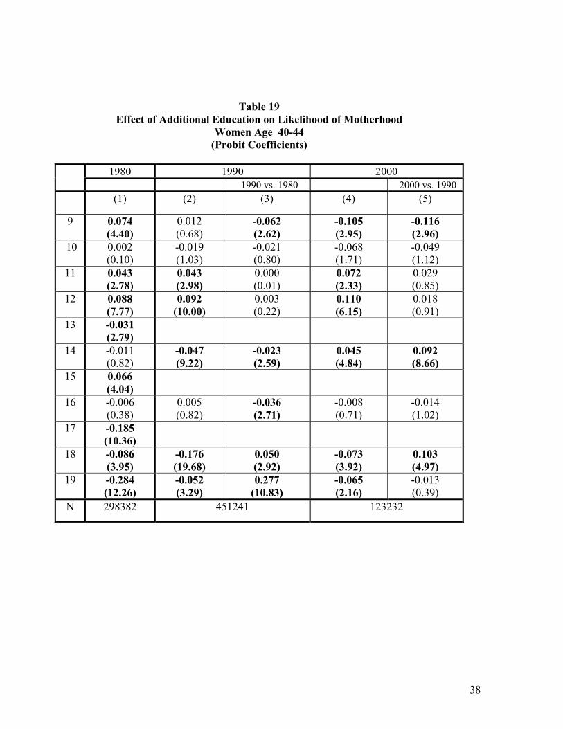
between education and motherhood for women age 40-44. Figure 15 and Table 18 indicates that there
was indeed a tradeoff between motherhood and marriage for women with more than a college degree.
81.5 percent of women with 16 years of education were mothers at age 40-44, while only 63.4 percent
of women with a professional degree or doctorate had children. However, as with marriage, the
difference fell in each of the two subsequent decades, from 18.1 percentage points in 1980, to 8.0 (73.0
– 65.0) percentage points in 1990, and then to 4.9 (71.2 - 66.3) percentage points in 2000. These
declines are statistically significant. The effect of having a master’s relative to a bachelor’s degree
became weaker in the 1980’s (t=2.92) and the 1990’s (t=4.97). The effect of having a doctorate or
professional degree became significantly weaker in the 1980’s (t=10.83).
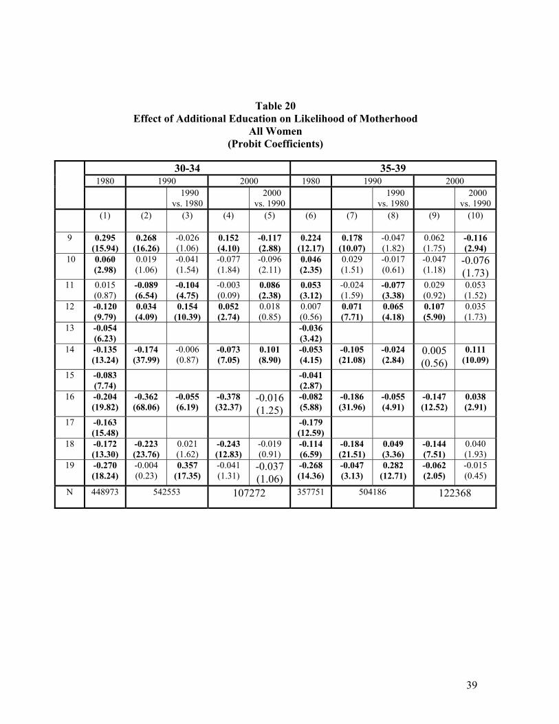
Because the children of women age 40-44 may no longer be co-resident, motherhood will tend
to be understated for this age group, in particular. The compression in these profiles may be explained
by the fact that the tendency for more educated women to postpone childbearing has increased. To
examine this possibility, In Figures 18-20 I plot the relationship between education and motherhood for
women age 30-34 and 35-39. If the compression were due solely to differential changes in timing, the
12 Because there is no information on prior cohabitations, it is not possible to construct a measure of married/cohabiting comparable to “Ever”.
16
negative relationship between education and motherhood over the range would have increased over the
period. However, this is not the case.
III.E. Reconciling these Results with the Literature and Perceptions
What explains the differences between the perceptions of the existence of a success penalty,
and the findings of authors such as Goldin and Hewlett - and these findings? First, other researchers
have characterized “success” in terms of income, while this paper looks at education. It may be that
there is limited scope for even highly educated women to translate their education to income if they are
married. The next step in this study would be to repeat this analysis using labor income, as well as
education, as the explanatory variable.
Second, “college educated” is a heterogeneous category in terms of marriage market outcomes.
Goldin focused on women college graduates, but could not distinguish by level of education beyond
sixteen years. However, in 1980, and to a lesser extent in 1990, there was a substantial success penalty
for education beyond college graduation.
Third, Goldin focuses on motherhood as the outcome reflecting success in terms of family,
while this paper focuses on marriage. While there still exists a quantitatively and statistically
significant tradeoff between education and motherhood at higher levels of education, this dimension of
the success premium has also appeared to decline over the period. Of course, the measure of
motherhood available from the Census is imperfect.
Fourth, there has been a significant decline in the likelihood of marriage at virtually all levels.
The resonance of Hewlett’s work with readers of the New York Times may reflect an awareness of the
reduced likelihood of marriage overall, combined with a focus on the higher end of the education
distribution which tends to read the Times.
Finally, the elimination of the success premium is a recent phenomenon. Goldin describes five
cohorts of women graduating college over the period 1900 to 1995. Women in Cohort I (graduating
year 1900 to 1919), primarily became teachers, and were unlikely to get married. Women in Cohort III
17
(graduating 1946 to 1965) had both family and career, but college attendance for this group was aimed
at accessing the market of college educated men, and were unlikely to have both career and family
simultaneously. Women in Cohort IV (graduating 1966 to 1979) the last cohort for which Goldin has
completed fertility data, report having desired motherhood and career, but only about 17 percent had
achieved that by 1988. Perhaps what we are seeing in the 2000 data, where the success penalty in
terms of marriage is virtually eliminated, and the success penalty in terms of motherhood is declining,
is the emergence of a cohort of women for whom the combination of career and motherhood is not
impossible. This would be consistent with the report that 71 percent of women attending a recent
Fortune magazine study of 187 women attending FORTUNE Magazine’s Most Powerful Women in
Business Summit were mothers (Sellers, 2002).
IV. Conclusions and Directions for Future Research
The relationship between education and marriage for women age 40-44 was an inverted U in
1980. The profile shifted down and became flatter in each of the two subsequent decades, and the
“success penalty”, measured as the difference between the peak of the profile and the likelihood of
marriage at the highest level of education, fell substantially in each of the subsequent two decades.
The penalty in terms of motherhood, a well as marriage appears to be falling as well. For men, the
profiles were essentially flat in 1980, but shifted down and became steeper in each of the subsequent
two decades.
What are the implications of these results? First, the decline in marriage is overwhelmingly a
phenomenon of the less educated segments of the population, particularly among blacks. This reflects
Wilson’s [1987] work regarding the declining number of marriageable low-skilled men due to the
decline in their labor market opportunities over the period.
Second, the findings suggest that the “decline in hypergamy” effect outweighs the “excess
supply effect”, suggesting that the marriage market is accommodating the increased number of
18
successful women competing for appropriate men by reducing the asymmetry between husbands’ and
wives’ characteristics at the time of marriage.
Finally, the perception that women face a stark choice between career and marriage is incorrect.
Young women no longer need to feel pressure to limit investments in their careers in order to enhance
their opportunities in terms of marriage, and perhaps motherhood.
Still, the issue of the relationship between marriage and career is extremely complicated, and
further work remains on the agenda. One caveat regarding causality must be considered in evaluating
these results. The changing relationship between education and marriage may reflect a shift in the
relationship between unobservables associated with marriage and education. For instance, as the later
cohort of women included more women with higher education, they may be less selective with respect
to the preferences and/or endowments which would generate lower likelihood of marriage. This
would tend to lead to a more positive relationship between education and marriage in the later years,
and suggest that the perceived “success penalty” in the early years was a choice, not the result of
education per se. Also, education may respond to marriage itself – with women in the later cohorts
being more likely to remain in school while married. The latter issue can be addressed with a panel
data set which tracks the marital and education histories of respondents.
Other tasks include continuing to reconcile these results with other papers in the literature.
This will involve obtaining more precise measures of motherhood, and tracking these outcomes with
respect to income as well as education. Other data sets can be consulted in order to obtain more
reliable causal estimates of the effect of education and career investments on family outcomes, using
sibling and instrumental variables techniques. This will also make it possible to uncover the
circumstances under which women are able to combine career and family. Finally, I will use the
Census data estimate changes in assortative mating and hypergamy directly, by tracking the change in
the relationship between husbands’ and wives’ characteristics over time.
19
References
Becker, Gary S. (1973) “A Theory of Marriage: Part I” Journal of Political Economy 81:4, 813-46. Becker , Gary S. (1974) “A Theory of Marriage: Part II” Journal of Political Economy 82:2, S11-S26. Becker, Gary S. (1981) A Treatise on the Family (Cambridge: Harvard University Press). Becker, Gary S. (1985) “Human Capital, Effort, and the Sexual Division of Labor” Journal of Labor Economics 81:4, 813-46. Behrman, Jere and Mark R. Rosenzweig (2002) “Does Increasing Women’s Schooling Raise the Schooling of the Next Generation?” American Economic Review 92:1, 323-34. Blau, Francine D. (1998) “Trends in the Well-Being of American Women, 1970-1995, Journal of Economic Literature 36 (Section I). Bumpass, L. L., J.J. Sweet and Andrew Cherlin (1991) “The Role of Cohabitation in Declining Rates of Marriage” Journal of Marriage and the Family 53, 913-27. Casper, Lynne M, Philip N. Cohen and Tavia Simmons (1999) “How Does POSSLQ Measure Up? Historical Estimates of Cohabitation,” Population Division Working Paper No. 36, US Bureau of the Census, May 1999. Dowd, Maureen (2002) “The Baby Bust”, The New York Times, April 10, 2002. Goldstein, Joshua R. and Catherine T. Kenney (2001) “Marriage Delayed or Marriage Forgone? New Cohort Forecasts of First Marriage for U.S. Women” American Sociological Review 66, 506-519. Gray, Jeffrey S. (1997) “The Fall in Men's Return to Marriage: Declining Productivity Effects or Changing Selection?” Journal of Human Resources 32:3, 481-504. Hewlett, Sylvia (2002) Creating a Life: Professional Women and the Quest for Children, New York: Hyperion. Hungerford, Thomas and Gary Solon (1987) “Sheepskin Effects in the Returns to Education,” Review of Economics and Statistics 69:1, 175-77. Jacobsen, Joyce, (1998) The Economics of Gender, New York: Blackwell. Juhn, Chinhui (1992) “The Decline in Male Labor Force Participation: The Role of Declining Opportunities,” Quarterly Journal of Economics 107, p. 79-102. Lam, David (1988) “Marriage Markets and Assortative Mating with Household Public Goods: Theoretical Results and Empirical Implications” Journal of Human Resources 23(4) 462-87. Lundberg, Shelly and Robert A. Pollak (1995) “Bargaining and Distribution in Marriage” Journal of Economic Perspectives 10:4, 139-58. Lundberg, Shelly and Elaina Rose (1998) “The Determinants of Specialization within Marriage”,
20
mimeo, University of Washington. Mare, Robert (1991) “Five Decades of Educational Assortative Mating, American Sociological Review 56 15-32. Miller, Barbara (1981)The Endangered Sex : Neglect of Female Children in Rural North India, London: Cornell University. Naidich, Andrew (2002), Letter to the Editor, The New York Times April 12, 2002. Pencavel, John (1998) “Assortative Mating by Schooling and the Work Behavior of Wives and Husbands” American Economic Review 88:2, 326-29. Qian , Zhenchao (1998) “Changes in Assortative Mating: The Impact of Age and Education, 1970-1990” Demography 35:3, 279-92. Rose, Elaina (2001) “Marriage and Assortative Mating: How Have the Patterns Changed?” mimeo, University of Washington. http://www.econ.washington.edu/people/detail.asp?uid=erose. Sellers, Patricia (2002) “Not All Women Cry the Baby Blues”, FORTUNE, April 29, 2002.
21
Figure 1: Percent Currently Married (All Women, Age 40-44)edu
80 currmar_f_40 90 currmar_f_40 100 currmar_f_40
8 9 10 11 12 13 14 15 16 17 18 19
.64381
.831818
Figure 2: Percent Ev er Married (All Women, Age 40-44)edu
80 evermar_f_40 90 evermar_f_40 100 evermar_f_40
8 9 10 11 12 13 14 15 16 17 18 19
.823264
.961674
Figure 3: Percent Currently Married (All Men, Age 40-44)edu
80 currmar_m_40 90 currmar_m_40 100 currmar_m_40
8 9 10 11 12 13 14 15 16 17 18 19
.625631
.861557
Figure 4: Percent Ev er Married (All Men, Age 40-44)edu
80 evermar_m_40 90 evermar_m_40 100 evermar_m_40
8 9 10 11 12 13 14 15 16 17 18 19
.79366
.950506
Figure 5: Percent Currently Married (White Women, Age 40-44)edu
80 currmar_f_40 90 currmar_f_40 100 currmar_f_40
8 9 10 11 12 13 14 15 16 17 18 19
.660184
.849837
Figure 6: Percent Ev er Married (White Women, Age 40-44)edu
80 evermar_f_40 90 evermar_f_40 100 evermar_f_40
8 9 10 11 12 13 14 15 16 17 18 19
.806754
.979254
Figure 7: Percent Currently Married (Black Women, Age 40-44)edu
80 currmar_f_40 90 currmar_f_40 100 currmar_f_40
8 9 10 11 12 13 14 15 16 17 18 19
.396277
.703526
Figure 8: Percent Ev er Married (Black Women, Age 40-44)edu
80 evermar_f_40 90 evermar_f_40 100 evermar_f_40
8 9 10 11 12 13 14 15 16 17 18 19
.574468
.913656
22
Figure 9: Percent Currently Married (White Men, Age 40-44)edu
80 currmar_m_40 90 currmar_m_40 100 currmar_m_40
8 9 10 11 12 13 14 15 16 17 18 19
.646021
.871054
Figure 10: Percent Ev er Married (White Men, Age 40-44)edu
80 evermar_m_40 90 evermar_m_40 100 evermar_m_40
8 9 10 11 12 13 14 15 16 17 18 19
.780699
.955561
Figure 11: Percent Currently Married (Black Men, Age 40-44)edu
80 currmar_m_40 90 currmar_m_40 100 currmar_m_40
8 9 10 11 12 13 14 15 16 17 18 19
.461066
.783133
Figure 12: Percent Ev er Married (Black Men, Age 40-44)edu
80 evermar_m_40 90 evermar_m_40 100 evermar_m_40
8 9 10 11 12 13 14 15 16 17 18 19
.585202
.915647
Figure 13: Percent Married/Cohabiting (All Women, Age 40-44)edu
80 currpos_f_40 90 currpos_f_40 100 currpos_f_40
8 9 10 11 12 13 14 15 16 17 18 19
.674629
.839194
Figure 14: Percent Married/Cohabiting (All Men, Age 40-44)edu
80 currpos_m_40 90 currpos_m_40 100 currpos_m_40
8 9 10 11 12 13 14 15 16 17 18 19
.686869
.872135
23
Figure 15: Proportion Mothers (All Women, Age 40-44)edu
80 parfrac2_f_40 90 parfrac2_f_40 100 parfrac2_f_40
8 9 10 11 12 13 14 15 16 17 18 19
.632754
.817023
Figure 16: Proportion Mothers (All Women, Age 35-39)edu
80 parfrac2_f_35 90 parfrac2_f_35 100 parfrac2_f_35
8 9 10 11 12 13 14 15 16 17 18 19
.620572
.860717
Figure 17: Proportion Mothers (All Women, Age 30-34)edu
80 parfrac2_f_30 90 parfrac2_f_30 100 parfrac2_f_30
8 9 10 11 12 13 14 15 16 17 18 19
.435562
.850115
Figure 18: Proportion Mothers (All Women, Age 40-44)edu
80 parfrac1_f_40 90 parfrac1_f_40 100 parfrac1_f_40
8 9 10 11 12 13 14 15 16 17 18 19
.630687
.817023
Figure 19: Proportion Mothers (All Women, Age 35-39)edu
80 parfrac1_f_35 90 parfrac1_f_35 100 parfrac1_f_35
8 9 10 11 12 13 14 15 16 17 18 19
.618865
.860717
Figure 20: Proportion Mothers (All Women, Age 30-34)edu
80 parfrac1_f_30 90 parfrac1_f_30 100 parfrac1_f_30
8 9 10 11 12 13 14 15 16 17 18 19
.435562
.850115
24
Table 1
Sample Statistics
Women Men 1980 1990 2000 1980 1990 2000 All Educationa 12.5
(2.5) 13.4 (2.5)
13.4 (2.4)
13.0 (3.0)
13.7 (2.7)
13.3 (2.5)
Currently Marriedb 80.8 75.2 71.5 84.8 78.8 71.7 Ever Marriedb 94.7 92.8 89.0 93.4 91.0 85.5 Currently Married or Cohabitingb 81.6 77.5 75.1 86.0 81.5 75.7 N 298392 451241 123232 285184 433806 117672 White Education 12.6
(2.4) 13.5 (2.4)
13.6 (2.3)
13.2 (2.9)
13.9 (2.7)
13.5 (2.4)
Currently Married 82.8 77.2 74.2 85.8 79.7 73.0 Ever Married 96.0 94.1 91.4 94.0 91.8 86.9 Currently Married or Cohabiting 83.5 79.4 77.8 86.8 82.3 76.7 N 250650 375956 95738 244044 368816 93100 Black Education 12.0
(2.4) 12.8 (2.4)
13.0 (2.1)
11.9 (2.7)
12.6 (2.5)
12.7 (2.2)
Currently Married 65.9 56.3 50.6 75.3 67.0 58.6 Ever Married 89.0 83.1 72.7 88.3 83.4 73.8 Currently Married or Cohabiting 67.2 59.1 54.8 77.5 71.3 64.5 N 33127 43754 14172 27343 35922 12005
All Mother (Age 40-44) 79.4 72.4 70.0 N 298392 451241 123232 Mother (Age 35-39) 83.2 75.4 73.4 N 357751 504186 122368 Mother (Age 30-34) 76.0 69.4 66.9 N 448973 542553 107272
a Measured as “Edu-2”, standard error in parentheses. b Percentage of total.
25
Table 2
Effect of Education on Likelihood of Marriage All Women Age 40-44
Probit coefficients; z-scores in parentheses, marginal effects in brackets
(1) (2) (3) (4) (5) (6) 1980 1980 1990 1990 vs. 1980 2000 2000 vs. 1990 Edu-1 Edu-2 Edu-2 Edu-2 Edu-2 Edu-2
Outcome: Currently Married (“Current”)
Coefficient on Education
-0.011 (10.70) [-.0031]
-0.011 (10.64) [-.0030]
0.001 (1.54)
[.00040]
0.012 (9.31)
0.019 (11.54) [.0063]
0.017 (9.62)
Outcome: Ever Married (“Ever”)
Coefficient on Education
-0.026 (17.83) [-.0028]
-0.026 (17.83) [-.0028]
-0.013 (12.22) [-.0018]
0.012 (6.77)
0.001 (0.40)
[.00015]
0.014 (6.25)
N = 298382 N = 451251 N = 123232
Table 3 Percentage Married, by Education Level
All Women, Age 40-44
Education (Ed-2)
Currently Married (Figure 1)
Ever Married (Figure 2)
Year 1980 1990 2000 1980 1990 2000 8 76.3 69.4 70.4 90.1 84.6 82.3 9 79.2 73.7 67.4 94.8 92.5 87.8 10 80.6 73.7 66.0 95.8 93.6 86.7 11 80.2 72.4 64.4 96.1 92.3 85.2 12 83.2 77.7 71.9 96.1 94.8 90.5 13 80.8 . . 96.2 . . 14 79.6 74.0 70.8 95.6 94.2 90.1 15 78.6 . . 95.1 . . 16 82.1 76.9 74.9 93.7 91.5 88.2 17 76.7 . . 90.5 . . 18 74.2 73.1 73.6 88.8 87.7 86.1 19 66.4 71.3 73.3 82.6 88.5 85.6
26
Table 4 Effect of Additional Education on Likelihood of Marriage
All Women Age 40-44 (Probit Coefficients)
Currently Married Ever Married 1980 1990 2000 1980 1990 2000 1990
vs. 1980 2000
vs. 1990 1990
vs. 1980 2000
vs. 1990 (1) (2) (3) (4) (5) (6) (7) (8) (9) (10)
9 0.096 (5.61)
0.126 (7.40)
0.031 (1.26)
-0.084 (2.34)
-0.210 (5.30)
0.338 (14.02)
0.419 (18.60)
0.081 (2.46)
0.236 (5.48)
-0.183 (3.76)
10 0.051 (2.76)
-0.001 (0.05)
-0.052 (1.97)
-0.038 (0.96)
-0.037 (0.85)
0.107 (3.86)
0.082 (3.10)
-0.026 (0.67)
-0.051 (1.03)
-0.132 (2.37)
11 -0.015 (0.94)
-0.039 (2.68)
-0.025 (1.14)
-0.044 (1.41)
-0.004 (0.13)
0.030 (1.22)
-0.093 (4.45)
-0.124 (3.79)
-0.069 (1.83)
0.024 (0.56)
12 0.114 (9.80)
0.167 (18.07)
0.054 (3.62)
0.211 (11.86)
0.044 (2.18)
-0.004 (0.24)
0.198 (15.23)
0.202 (8.94)
0.265 (12.29)
0.067 (2.67)
13 -0.093 (8.29)
0.011 (0.63)
14 -0.042 (3.00)
-0.119 (22.95)
0.009 (0.96)
-0.033 (3.51)
0.086 (8.04)
-0.066 (3.01)
-0.052 (6.71)
-0.008 (0.55)
-0.023 (1.89)
0.029 (2.01)
15 -0.036 (2.25)
-0.050 (2.06)
16 0.127 (7.89)
0.092 (14.02)
0.008 (0.60)
0.125 (10.34)
0.032 (2.34)
-0.121 (5.21)
-0.202 (22.58)
-0.021 (1.13)
-0.101 (6.78)
0.102 (5.88)
17 -0.190 (10.56)
-0.224 (9.76)
18 -0.078 (3.56)
-0.120 (12.98)
0.106 (6.15)
-0.039 (2.03)
0.081 (3.80)
-0.092 (3.39)
-0.209 (18.38)
0.059 (2.67)
-0.101 (4.49)
0.109 (4.32)
19 -0.228 (9.74)
-0.053 (3.23)
0.216 (8.29)
-0.009 (0.29)
0.044 (1.23)
-0.279 (10.14)
0.039 (1.96)
0.367 (11.78)
-0.021 (0.58)
-0.061 (1.46)
N 298382 451241 123232 298382 451241 123232
27
Table 5
Effect of Education on Likelihood of Marriage All Men Age 40-44
Probit coefficients; z-scores in parentheses, marginal effects in brackets
(1) (2) (3) (4) (5) (6) 1980 1980 1990 1990 vs. 1980 2000 2000 vs.
1990 Edu-1 Edu-2 Edu-2 Edu-2 Edu-2 Edu-2
Outcome: Currently Married (“Current”)
Coefficient on Education
0.018 (18.24) [.0040]
0.017 (18.27) [.0040]
0.037 (46.60) [.011]
0.019 (15.72)
0.053 (33.48) [.018]
0.016 (9.28)
Outcome: Ever Married (“Ever”)
Coefficient on Education
0.021 (17.44) [.0027]
0.021 (17.52) [.0027]
0.027 (27.97) [.0044]
0.00097 (4.0)
0.034 (18.70) [.0077]
0.007 (3.37)
285184 433806 117672
Table 6 Percentage Married, by Education Level
All Men, Age 40-44
Education Currently Married (Figure 3)
Ever Married (Figure 4)
Year 1980 1990 2000 1980 1990 2000 8 79.6 71.9 68.9 87.8 82.2 79.4 9 82.2 74.8 65.4 92.1 89.5 82.5 10 83.0 75.0 62.6 93.0 90.0 80.5 11 83.5 72.8 62.8 93.8 88.9 80.5 12 86.0 77.9 69.4 94.4 91.9 85.6 13 85.8 . . 95.1 . . 14 85.5 79.1 72.4 94.7 92.4 86.8 15 84.9 . . 94.0 . . 16 85.9 80.9 77.7 93.7 90.7 86.8 17 85.3 . . 93.2 . . 18 86.2 83.1 80.4 93.5 91.4 87.5 19 85.4 84.6 82.7 92.8 92.4 89.3
28
Table 7
Effect of Additional Education on Likelihood of Marriage All Men Age 40-44 (Probit Coefficients)
Currently Married Ever Married 1980 1990 2000 1980 1990 2000 1990
vs. 1980 2000
vs. 1990 1990
vs. 1980 2000
vs. 1990 (1) (2) (3) (4) (5) (6) (7) (8) (9) (10)
9 0.099 (5.66)
0.086 (4.98)
-0.013 (0.54)
-0.098 (2.96)
-0.184 (4.93)
0.247 (11.59)
0.328 (15.83)
0.082 (2.74)
0.116 (3.11)
-0.212 (4.98)
10 0.030 (1.52)
0.006 (0.32)
-0.024 (0.85)
-0.076 (2.09)
-0.082 (1.99)
0.069 (2.74)
0.028 (1.14)
-0.041 (1.17)
-0.076 (1.83)
-0.104 (2.16)
11 0.020 (1.09)
-0.065 (4.14)
-0.085 (3.53)
0.007 (0.27)
0.073 (2.28)
0.060 (2.50)
-0.061 (3.08)
-0.120 (3.89)
-0.001 (0.02)
0.060 (1.62)
12 0.106 (7.57)
0.161 (15.78)
0.054 (3.14)
0.180 (11.16)
0.020 (1.04)
0.055 (2.98)
0.175 (13.82)
0.120 (5.36)
0.202 (11.03)
0.026 (1.18)
13 -0.011 (0.83)
0.056 (2.99)
14 -0.014 (0.83)
0.041 (7.11)
0.068 (6.67)
0.086 (8.61)
0.044 (3.85)
-0.030 (1.35)
0.039 (5.17)
0.021 (1.55)
0.056 (4.75)
0.017 (1.19)
15 -0.024 (1.38)
-0.066 (2.93)
16 0.042 (2.50)
0.063 (9.63)
0.043 (3.28)
0.169 (12.87)
0.106 (7.24)
-0.025 (1.17)
-0.112 (13.68)
-0.029 (1.71)
0.000 (0.01)
0.112 (6.50)
17 -0.026 (1.51)
-0.040 (1.87)
18 0.039 (1.86)
0.086 (9.11)
0.093 (5.55)
0.093 (4.34)
0.007 (0.28)
0.029 (1.10)
0.039 (3.45)
0.065 (3.15)
0.035 (1.47)
-0.004 (0.14)
19 -0.035 (1.82)
0.061 (4.63)
0.076 (3.70)
0.086 (2.89)
0.025 (0.77)
-0.060 (2.54)
0.072 (4.51)
0.117 (4.68)
0.093 (2.77)
0.021 (0.57)
N 285184 433806 117672 285184 433806 117672
29
Table 8
Percentage Married, by Education Level White Women, Age 40-44
Education Currently Married
(Figure 5) Ever Married
(Figure 6) Year 1980 1990 2000 1980 1990 2000
8 78.3 69.1 68.0 90.7 84.6 80.7 9 82.4 76.7 69.0 96.7 95.6 91.9 10 83.9 78 69.8 97.5 96.8 91.9 11 83.9 77.5 70.1 97.9 96.1 91.7 12 85.0 79.8 74.8 96.8 96.0 93.2 13 82.8 . . 96.9 . . 14 81.1 75.9 73.6 96.1 95.2 92.4 15 80.4 . . 95.7 . . 16 83.4 77.7 76.8 94.2 92.0 89.3 17 77.7 . . 90.8 . . 18 74.3 73.9 74.6 88.6 88.0 86.3 19 66.0 71.3 73.8 81.9 88.8 86.1
Table 9 Percentage Married, by Education Level
Black Women, Age 40-44
Education Currently Married (Figure 9)
Ever Married (Figure 10)
Year 1980 1990 2000 1980 1990 2000 8 62.2 50.6 39.6 83.1 70.7 57.4 9 64.5 55.9 48.2 86.8 78.1 64.4 10 67.0 54.5 46.6 89.5 80.4 66.1 11 66.8 53.8 45.0 89.6 80.4 66.1 12 67.2 58.5 51.5 89.6 84.2 72.7 13 66.9 . . 91.4 . . 14 64.8 55.3 51.4 91.4 85.8 75.4 15 63.1 . . 90.2 . . 16 64.4 58.9 52.8 89.9 85.0 76.0 17 63.9 . . 87.7 . . 18 70.4 58.3 55.8 91.0 83.2 78.5 19 60.7 55.5 57.9 86.2 79.9 78.6
30
Table 10
Effect of Additional Education on Likelihood of Marriage White Women Age 40-44
(Probit Coefficients)
Currently Married Ever Married 1980 1990 2000 1980 1990 2000 1990
vs. 1980 2000
vs. 1990 1990
vs. 1980 2000
vs. 1990 (1) (2) (3) (4) (5) (6) (7) (8) (9) (10)
9 0.151 (7.27)
0.229 (10.77)
0.078 (2.62)
0.027 (0.58)
-0.202 (3.89)
0.511 (15.99)
0.691 (22.05)
0.181 (4.03)
0.530 (8.68)
0.181 (4.03)
10 0.057 (2.58)
0.044 (1.95)
-0.013 (0.40)
0.023 (0.46)
-0.021 (0.38)
0.511 (15.99)
0.149 (3.92)
0.031 (0.58)
0.001 (0.01)
0.031 (0.58)
11 0.003 (0.14)
-0.018 (0.98)
-0.020 (0.78)
0.009 (0.22)
0.026 (0.60)
0.086 (2.48)
-0.101 (3.27)
-0.187 (4.02)
-0.011 (0.20)
-0.187 (4.02)
12 0.044 (3.14)
0.080 (7.07)
0.037 (2.05)
0.140 (6.02)
0.060 (2.32)
-0.182 (7.01)
-0.004 (0.21)
0.178 (5.58)
0.106 (3.32)
0.178 (5.58)
13 -0.089 (7.16)
0.008 (0.41)
14 -0.065 (4.22)
-0.132 (23.06)
0.006 (0.58)
-0.035 (3.28)
0.097 (7.97)
-0.101 (4.02)
-0.088 (9.68)
-0.018 (1.13)
-0.059 (3.99)
-0.018 (1.13)
15 -0.027 (1.57)
-0.042 (1.54)
16 0.114 (6.49)
0.059 (8.30)
-0.011 (0.77)
0.099 (7.28)
0.040 (2.57)
-0.147 (5.66)
-0.262 (26.20)
-0.049 (2.41)
-0.190 (11.02)
-0.049 (2.41)
17 -0.207 (10.68)
-0.248 (9.93)
18 -0.110 (4.65)
-0.122 (12.30)
0.137 (7.36)
-0.068 (3.23)
0.054 (2.29)
-0.121 (4.15)
-0.231 (18.79)
0.075 (3.16)
-0.148 (5.96)
0.075 (3.16)
19 -0.238 (9.42)
-0.078 (4.47)
0.218 (7.72)
-0.025 (0.72)
0.054 (1.37)
-0.294 (9.93)
0.042 (1.94)
0.399 (11.86)
-0.011 (0.27)
0.399 (11.86)
N 250650 375956 95738 250650 375956 95738
31
Table 11 Effect of Additional Education on Likelihood of Marriage
Black Women Age 40-44 (Probit Coefficients)
Currently Married Ever Married 1980 1990 2000 1980 1990 2000 1990
vs. 1980 2000
vs. 1990 1990
vs. 1980 2000
vs. 1990 (1) (2) (3) (4) (5) (6) (7) (8) (9) (10)
9 0.060 (1.57)
0.134 (3.08)
0.074 (1.28)
0.218 (2.13)
0.085 (0.76)
0.157 (3.40)
0.232 (4.89)
0.074 (1.12)
0.182 (1.76)
-0.050 (0.44)
10 0.070 (1.76)
-0.037 (0.83)
-0.106 (1.80)
-0.040 (0.40)
-0.003 (0.03)
0.135 (2.70)
0.079 (1.59)
-0.056 (0.80)
0.046 (0.46)
-0.032 (0.28)
11 -0.006 (0.19)
-0.019 (0.59)
-0.013 (0.27)
-0.041 (0.61)
-0.023 (0.30)
0.010 (0.23)
0.001 (0.02)
-0.009 (0.17)
-0.001 (0.01)
-0.001 (0.02)
12 0.012 (0.48)
0.120 (5.86)
0.108 (3.40)
0.163 (4.35)
0.043 (1.00)
-0.004 (0.11)
0.147 (6.17)
0.150 (3.78)
0.187 (4.81)
0.041 (0.89)
13 -0.008 (0.29)
0.106 (2.61)
14 -0.058 (1.48)
-0.082 (5.25)
-0.028 (1.09)
-0.002 (0.07)
0.080 (2.65)
0.001 (0.01)
0.069 (3.66)
-0.020 (0.60)
0.086 (3.07)
0.016 (0.48)
15 -0.046 (0.99)
-0.072 (1.15)
16 0.034 (0.69)
0.093 (3.93)
0.118 (2.69)
0.035 (0.94)
-0.058 (1.32)
-0.015 (0.23)
-0.034 (1.19)
0.036 (0.64)
0.017 (0.43)
0.051 (1.04)
17 -0.011 (0.19)
-0.115 (1.51)
18 0.178 (2.44)
-0.017 (0.49)
-0.090 (1.52)
0.075 (1.16)
0.092 (1.26)
0.181 (1.91)
-0.076 (1.90)
-0.043 (0.57)
0.083 (1.16)
0.159 (1.93)
19 -0.264 (3.40)
-0.072 (1.11)
0.099 (1.06)
0.055 (0.46)
0.127 (0.94)
-0.252 (2.53)
-0.123 (1.68)
0.031 (0.27)
0.005 (0.03)
0.128 (0.84)
N 33127 43754 14172 33127 43754 14172
32
Table 12 Percentage Married, by Education Level
White Men, Age 40-44
Education Currently Married (Figure 7)
Ever Married (Figure 8)
Year 1980 1990 2000 1980 1990 2000 8 80.1 70.1 64.6 88.2 81.7 78.1 9 83.9 76.8 66.0 93.1 92.1 85.3 10 84.8 77.3 65.1 94.5 92.6 84.7 11 85.6 75.2 65.0 95.2 91.5 84.8 12 87.1 79.2 70.9 95.1 92.9 87.3 13 86.9 . . 95.6 . . 14 86.1 79.8 73.4 95.0 92.9 87.7 15 85.8 . . 94.2 . . 16 86.2 81.0 78.2 93.9 90.9 87.1 17 85.8 . . 93.3 . . 18 86.5 83.2 80.6 93.8 91.4 87.4 19 85.1 84.5 82.5 92.6 92.4 89.3
Table 13
Percentage Married, by Education Level Black Men, Age 40-44
Education Currently Married
(Figure 11) Ever Married
(Figure 12) Year 1980 1990 2000 1980 1990 2000
8 71.5 56.6 47.1 82.3 69.8 58.5 9 74.7 62.0 51.6 87.1 76.8 62.5 10 74.7 61.9 46.1 86.4 78.3 60.9 11 76.4 63.4 51.9 88.7 80.7 66.4 12 76.4 66.5 57.2 89.3 83.8 72.9 13 77.1 . . 91.6 . . 14 75.9 70.1 62.4 91.0 87.5 79.2 15 76.3 . . 91.4 . . 16 75.4 72.8 69 89.2 87.1 82.1 17 73.5 . . 90.0 . . 18 76.4 74.6 70.3 89.4 87.8 85.3 19 78.3 76.3 73.9 91.3 89.4 81.7
33
Table 14
Effect of Additional Education on Likelihood of Marriage White Men Age 40-44 (Probit Coefficients)
Currently Married Ever Married 1980 1990 2000 1980 1990 2000 1990
vs. 1980 2000
vs. 1990 1990
vs. 1980 2000
vs. 1990 (1) (2) (3) (4) (5) (6) (7) (8) (9) (10)
9 0.143 (7.02)
0.205 (9.95)
0.062 (2.15)
0.039 (0.92)
-0.167 (3.58)
0.303 (12.03)
0.507 (19.38)
0.203 (5.60)
0.275 (5.70)
-0.231 (4.21)
10 0.038 (1.65)
0.014 (0.61)
-0.024 (0.73)
-0.026 (0.58)
-0.040 (0.80)
0.108 (3.61)
0.036 (1.18)
-0.072 (1.67)
-0.026 (0.50)
-0.062 (1.03)
11 0.034 (1.59)
-0.068 (3.61)
-0.102 (3.58)
-0.003 (0.08)
0.065 (1.69)
0.075 (2.55)
-0.074 (2.94)
-0.148 (3.85)
0.003 (0.07)
0.077 (1.62)
12 0.070 (4.26)
0.133 (10.91)
0.063 (3.09)
0.167 (8.36)
0.033 (1.43)
-0.017 (0.76)
0.095 (5.90)
0.112 (4.03)
0.113 (4.79)
0.019 (0.65)
13 -0.010 (0.68)
0.050 (2.37)
14 -0.034 (1.94)
0.023 (3.65)
0.062 (5.61)
0.075 (6.75)
0.052 (4.07)
-0.053 (2.16)
0.004 (0.44)
0.012 (0.81)
0.021 (1.56)
0.017 (1.09)
15 -0.017 (0.90)
-0.077 (3.16)
16 0.020 (1.12)
0.043 (6.19)
0.045 (3.21)
0.152 (10.52)
0.109 (6.79)
-0.027 (1.18)
-0.138 (15.81)
-0.039 (2.16)
-0.030 (1.79)
0.108 (5.73)
17 -0.021 (1.14)
-0.043 (1.90)
18 0.033 (1.49)
0.083 (8.31)
0.087 (4.92)
0.085 (3.63)
0.002 (0.09)
0.034 (1.21)
0.032 (2.66)
0.059 (2.67)
0.015 (0.58)
-0.017 (0.58)
19 -0.061 (3.04)
0.053 (3.84)
0.097 (4.52)
0.072 (2.20)
0.019 (0.54)
-0.087 (3.49)
0.066 (3.93)
0.135 (5.14)
0.098 (2.63)
0.032 (0.78)
N 244044 368816 93100 244044 368816 93100
34
Table 15 Effect of Additional Education on Likelihood of Marriage
Black Men Age 40-44 (Probit Coefficients)
Currently Married Ever Married 1980 1990 2000 1980 1990 2000 1990
vs. 1980 2000
vs. 1990 1990
vs. 1980 2000
vs. 1990 (1) (2) (3) (4) (5) (6) (7) (8) (9) (10)
9 0.097 (2.35)
0.138 (3.14)
0.040 (0.67)
0.112 (1.14)
-0.025 (0.24)
0.206 (4.32)
0.214 (4.55)
0.007 (0.11)
0.103 (1.04)
-0.110 (1.00)
10 0.000 (0.01)
-0.003 (0.06)
-0.003 (0.05)
-0.137 (1.41)
-0.134 (1.25)
-0.036 (0.67)
0.047 (0.93)
0.083 (1.13)
-0.043 (0.44)
-0.090 (0.81)
11 0.054 (1.37)
0.040 (1.16)
-0.014 (0.27)
0.146 (2.24)
0.106 (1.43)
0.114 (2.43)
0.086 (2.23)
-0.028 (0.46)
0.147 (2.22)
0.061 (0.80)
12 -0.000 (0.00)
0.083 (3.61)
0.083 (2.15)
0.133 (3.61)
0.051 (1.16)
0.035 (0.93)
0.121 (4.66)
0.087 (1.91)
0.189 (4.92)
0.068 (1.46)
13 0.024 (0.65)
0.131 (2.69)
14 -0.042 (0.87)
0.103 (5.60)
0.102 (3.30)
0.134 (4.57)
0.032 (0.91)
-0.035 (0.56)
0.163 (7.43)
0.049 (1.26)
0.202 (6.31)
0.040 (1.02)
15 0.013 (0.25)
0.022 (0.32)
16 -0.028 (0.51)
0.078 (2.91)
0.111 (2.22)
0.180 (3.86)
0.102 (1.89)
-0.128 (1.82)
-0.017 (0.54)
0.106 (1.72)
0.107 (2.05)
0.124 (2.03)
17 -0.057 (0.84)
0.043 (0.51)
18 0.092 (1.09)
0.055 (1.27)
0.069 (0.98)
0.037 (0.44)
-0.018 (0.19)
-0.030 (0.29)
0.031 (0.61)
0.002 (0.03)
0.129 (1.34)
0.097 (0.89)
19 0.062 (0.75)
0.055 (0.84)
-0.055 (0.58)
0.108 (0.87)
0.053 (0.37)
0.108 (1.06)
0.084 (1.06)
-0.008 (0.07)
-0.146 (1.06)
-0.230 (1.45)
N 27343 35922 12005 27343 35922 12005
35
Table 16
Percentage Currently Married or Cohabiting, by Education Level Individuals Age 40-44
Education All Women
(Figure 15) All Men
(Figure 16) Year 1980 1990 2000 1980 1990 2000
8 77.1 71.9 73.4 80.6 74.8 72.7 9 80 76.8 72.3 83.6 78.2 71.2 10 81.7 77.1 72.1 84.4 79.1 68.7 11 81.2 75.6 70 84.9 77 68.7 12 83.9 80 76 87.1 81 74.2 13 81.7 . . 87 . . 14 80.4 76.4 74.4 86.7 82 76.2 15 79.4 . . 86.1 . . 16 82.6 78.6 77.1 86.9 82.8 80 17 77.3 . . 86.2 . . 18 74.9 74.7 75.4 87.2 84.8 81.8 19 67.5 73.4 75.8 86.4 86.5 85.1
36
Table 17 Effect of Additional Education on Likelihood of Current Marriage of Cohabitation
Individuals Age 40-44 (Probit Coefficients)
All Women All Men 1980 1990 2000 1980 1990 2000 1990
vs. 1980 2000
vs. 1990 1990
vs. 1980 2000
vs. 1990 (1) (2) (3) (4) (5) (6) (7) (8) (9) (10)
9 0.099 (5.76)
0.154 (8.85)
0.055 (2.25)
0.154 (8.85)
0.055 (2.25)
0.115 (6.46)
0.110 (6.23)
-0.005 (0.18)
-0.043 (1.27)
-0.153 (4.00)
10 0.063 (3.39)
0.007 (0.39)
-0.056 (2.08)
0.007 (0.39)
-0.056 (2.08)
0.034 (1.68)
0.031 (1.54)
-0.003 (0.09)
-0.071 (1.91)
-0.103 (2.41)
11 -0.021 (1.29)
-0.049 (3.27)
-0.029 (1.30)
-0.049 (3.27)
-0.029 (1.30)
0.022 (1.20)
-0.072 (4.41)
-0.094 (3.80)
-0.001 (0.03)
0.071 (2.17)
12 0.107 (9.15)
0.152 (16.01)
0.045 (2.95)
0.152 (16.01)
0.045 (2.95)
0.098 (6.85)
0.141 (13.43)
0.043 (2.42)
0.162 (9.77)
0.021 (1.05)
13 -0.087 (7.68)
-0.003 (0.20)
14 -0.047 (3.36)
-0.125 (23.59)
0.000 (0.05)
-0.125 (23.59)
0.000 (0.05)
-0.015 (0.92)
0.036 (5.95)
0.056 (5.38)
0.064 (6.25)
0.028 (2.39)
15 -0.036 (2.23)
-0.028 (1.60)
16 0.118 (7.29)
0.075 (11.18)
0.001 (0.08)
0.075 (11.18)
0.001 (0.08)
0.035 (2.04)
0.033 (4.95)
0.024 (1.81)
0.127 (9.43)
0.094 (6.23)
17 -0.191 (10.60)
-0.028 (1.62)
18 -0.077 (3.48)
-0.128 (13.72)
0.099 (5.68)
-0.128 (13.72)
0.099 (5.68)
0.045 (2.13)
0.080 (8.26)
0.086 (5.04)
0.070 (3.19)
-0.011 (0.45)
19 -0.219 (9.31)
-0.041 (2.48)
0.218 (8.30)
-0.041 (2.48)
0.218 (8.30)
-0.040 (2.06)
0.075 (5.53)
0.092 (4.39)
0.132 (4.30)
0.057 (1.69)
N 298308 450977 123232 285041 433427 117672
37
Table 18 Percentage Mothers, by Education Level
All Women, by Age
Education Age 40-44 Age 35-39 Age 30-44 Year 1980 1990 2000 1980 1990 2000 1980 1990 2000
8 75 70.1 69.6 77.4 71.7 70.4 74.8 68.4 68.7 9 77.3 70.5 65.8 83.6 77.4 72.5 83.2 77.3 73.8 10 77.3 69.8 63.3 84.7 78.3 70.9 84.7 77.8 71.3 11 78.6 71.3 65.9 85.9 77.6 71.9 85.0 75.1 71.1 12 81.1 74.3 69.9 86.1 79.6 75.4 82.0 76.2 72.9 13 80.2 . . 85.3 . . 80.6 . . 14 79.9 72.8 71.4 84 76.5 75.6 76.7 70.5 70.4 15 81.7 . . 83 . . 74.1 . . 16 81.5 73.0 71.2 80.8 70.5 70.7 67.1 57 56.3 17 76.2 . . 75.6 . . 61.0 . . 18 73.5 66.9 68.6 71.9 63.8 65.6 54.3 48.1 46.6 19 63.4 65.0 66.3 62.2 62.1 63.3 43.6 48.0 45.0
38
Table 19 Effect of Additional Education on Likelihood of Motherhood
Women Age 40-44 (Probit Coefficients)
1980 1990 2000 1990 vs. 1980 2000 vs. 1990 (1) (2) (3) (4) (5)
9 0.074 (4.40)
0.012 (0.68)
-0.062 (2.62)
-0.105 (2.95)
-0.116 (2.96)
10 0.002 (0.10)
-0.019 (1.03)
-0.021 (0.80)
-0.068 (1.71)
-0.049 (1.12)
11 0.043 (2.78)
0.043 (2.98)
0.000 (0.01)
0.072 (2.33)
0.029 (0.85)
12 0.088 (7.77)
0.092 (10.00)
0.003 (0.22)
0.110 (6.15)
0.018 (0.91)
13 -0.031 (2.79)
14 -0.011 (0.82)
-0.047 (9.22)
-0.023 (2.59)
0.045 (4.84)
0.092 (8.66)
15 0.066 (4.04)
16 -0.006 (0.38)
0.005 (0.82)
-0.036 (2.71)
-0.008 (0.71)
-0.014 (1.02)
17 -0.185 (10.36)
18 -0.086 (3.95)
-0.176 (19.68)
0.050 (2.92)
-0.073 (3.92)
0.103 (4.97)
19 -0.284 (12.26)
-0.052 (3.29)
0.277 (10.83)
-0.065 (2.16)
-0.013 (0.39)
N 298382 451241 123232
39
Table 20 Effect of Additional Education on Likelihood of Motherhood
All Women (Probit Coefficients)
30-34 35-39 1980 1990 2000 1980 1990 2000 1990
vs. 1980 2000
vs. 1990 1990
vs. 1980 2000
vs. 1990 (1) (2) (3) (4) (5) (6) (7) (8) (9) (10)
9 0.295 (15.94)
0.268 (16.26)
-0.026 (1.06)
0.152 (4.10)
-0.117 (2.88)
0.224 (12.17)
0.178 (10.07)
-0.047 (1.82)
0.062 (1.75)
-0.116 (2.94)
10 0.060 (2.98)
0.019 (1.06)
-0.041 (1.54)
-0.077 (1.84)
-0.096 (2.11)
0.046 (2.35)
0.029 (1.51)
-0.017 (0.61)
-0.047 (1.18)
-0.076 (1.73)
11 0.015 (0.87)
-0.089 (6.54)
-0.104 (4.75)
-0.003 (0.09)
0.086 (2.38)
0.053 (3.12)
-0.024 (1.59)
-0.077 (3.38)
0.029 (0.92)
0.053 (1.52)
12 -0.120 (9.79)
0.034 (4.09)
0.154 (10.39)
0.052 (2.74)
0.018 (0.85)
0.007 (0.56)
0.071 (7.71)
0.065 (4.18)
0.107 (5.90)
0.035 (1.73)
13 -0.054 (6.23)
-0.036 (3.42)
14 -0.135 (13.24)
-0.174 (37.99)
-0.006 (0.87)
-0.073 (7.05)
0.101 (8.90)
-0.053 (4.15)
-0.105 (21.08)
-0.024 (2.84)
0.005 (0.56)
0.111 (10.09)
15 -0.083 (7.74)
-0.041 (2.87)
16 -0.204 (19.82)
-0.362 (68.06)
-0.055 (6.19)
-0.378 (32.37)
-0.016 (1.25)
-0.082 (5.88)
-0.186 (31.96)
-0.055 (4.91)
-0.147 (12.52)
0.038 (2.91)
17 -0.163 (15.48)
-0.179 (12.59)
18 -0.172 (13.30)
-0.223 (23.76)
0.021 (1.62)
-0.243 (12.83)
-0.019 (0.91)
-0.114 (6.59)
-0.184 (21.51)
0.049 (3.36)
-0.144 (7.51)
0.040 (1.93)
19 -0.270 (18.24)
-0.004 (0.23)
0.357 (17.35)
-0.041 (1.31)
-0.037 (1.06)
-0.268 (14.36)
-0.047 (3.13)
0.282 (12.71)
-0.062 (2.05)
-0.015 (0.45)
N 448973 542553 107272 357751 504186 122368
40
Appendix I Details of Data Transformations
Table AI-1
Measuring Motherhood Using U.S. Census Data
1980 1990 2000 If Individual was head and household contained: Child of Head Maybea Parentb Parent b,d Grandchild of Head Maybea Maybec Maybe c Child-in-Law of Head Maybe a Maybec Maybe c Step-Child of Head NA Step Step If Individual was spouse of head and household contained:
Child of Head Maybe a Maybe Maybe Grandchild of Head Maybe a Maybe Maybe Child-in-Law of Head Maybe a Maybe Maybe Step-Child of Head NA Parent Parent If Individual was a Parent in Parent/Child Subfamilye Maybe Maybe Maybe If Individual was Parent, Grandparent, or Parent-in-Lawf of Head
Maybe Maybe Maybe
If there were multiple children with different relationships to the mother, she was assigned to the highest ranking category, pursuant to the following ranking: Parent Maybe Step Not Parent “Mother” includes Parent, Maybe and Step, and “Mother-2” includes Parent and Maybe. “Mother” is more comparable across years, but “Mother-2” is more precise for 1990 and 2000.
a “Child” and associated variables do not distinguish step- vs. biological relationships with respect to head in 1980. b Biological and step-children are distinguished in 1990 and 2000. d 2000 Census data distinguish biological and adopted children; both are treated as children in here. c Cannot distinguish grandchildren from step-grandchildren, and children-in-law from step children-in-law in 1990 and 2000. e Biological and step-relationships are not distinguished for subfamilies in any year. f Biological and step-relationships are not distinguished for parents, grandparents, and parents-in-law of head for any year.

41
Table AI-2
Measuring Education Using U.S. Census Data
1980 Code (Highest year of school
completed) (If attended but did not complete, then assigned
previous grade)
1990 Code: (Educational attainment)
2000 Code: (Educational attainment)
Edu-1
Edu-2
Never attended school Nursery school Kindergarten First grade Second grade Third grade Fourth grade Fifth grade Sixth grade Seventh grade Eighth grade
No school completed, Nursery school, Kindergarten, 1st, 2nd, 3rd, or 4th grade, 5th, 6th, 7th, or 8th grade
No school completed Nursery school to 4th grade 5th grade or 6th grade 7th grade or 8th grade
8 8
Ninth grade Ninth grade Ninth grade 9 9 Tenth grade Tenth grade Tenth grade 10 10 Eleventh grade Eleventh grade,
Twelfth grade, no diploma
Eleventh grade, Twelfth grade, no diploma
11 11
Twelfth grade High School graduate: diploma or GED
High School graduate: diploma or GED
12 12
First year of college 13 14 Second year of college Some college, but no
degree, Associate degree in college, occupational program,
Associate degree in college, academic program
Some college, but less than 1 year One or more years of college, no degree Associate degree
14 14
Third year of college 15 14 Fourth year college Bachelor’s degree Bachelor’s degree 16 16 Fifth year of college 17 16 Sixth year of college Master’s degree Master’s degree 18 18 Seventh year of college Eighth year of college
Professional degree Doctorate
Professional degree Doctorate
19 19


