
Do Expiring Budgets Lead to Wasteful Year-End Spending?
Evidence from Federal Procurement∗
Jeffrey B. Liebman and Neale Mahoney†
November 19, 2010
Abstract
Many organizations fund their spending out of a fixed budget that expires at year’s end.
Faced with uncertainty over future spending demands, these organizations have an incentive
to build a buffer stock of funds over the front end of the budget cycle. When demand does not
materialize, they then rush to spend these funds on lower quality projects at the end of the year.
We test these predictions using data on procurement spending by the U.S. federal government.
Using data on all federal contracts from 2004 through 2009, we document that spending spikes
in all major federal agencies during the 52nd week of the year as the agencies rush to exhaust
expiring budget authority. Spending in the last week of the year is 4.9 times higher than the
rest-of-the-year weekly average. We examine the relative quality of year-end spending using a
newly available dataset that tracks the quality of $130 billion in information technology (I.T.)
projects made by federal agencies. Consistent with the model, average project quality falls at
the end of the year. Quality scores in the last week of the year are 2.2 to 5.6 times more likely to
be below the central value. To explore the impact of allowing agencies to roll unused spending
over into subsequent fiscal years, we study the I.T. contracts of an agency with special authority
to roll over unused funding. We show that there is only a small end-of-year I.T. spending spike
in this agency and that the one major I.T. contract this agency issued in the 52nd week of the
year has a quality rating that is well above average.
∗We are grateful to Steven Kelman and Shelley Metzenbaum for conversations that stimulated our interest in thistopic. Mahoney acknowledges a Kapnick Fellowship and a Ric Weiland Fellowship for financial support.
†Liebman: Kennedy School of Government, Harvard University ([email protected]). Mahoney: Depart-ment of Economics, Stanford University ([email protected])

1 Introduction
Many organizations have budgets that expire at year’s end. In the U.S., most budget authority
provided to federal government agencies for discretionary spending requires the agencies to obli-
gate funds by the end of the fiscal year or return them to the Treasury general fund, and state and
municipal agencies typically face similar constraints (McPherson, 2007; Jones, 2005; GAO, 2004).1
For these organizations, unspent funding may not only represent a lost opportunity but can
also signal a lack of need to budget-setters, decreasing funding in future budget cycles (Lee and
Johnson, 1998; Jones, 2005). When current spending is explicitly used as the baseline in setting
budgets for the following year, this signaling effect is magnified.
This “use it or lose it” feature of time-limited budget authority has the potential to result in low
value spending—since the opportunity cost to organizations of spending about-to-expire funds is
effectively zero. Exacerbating this problem is the incentive to build up a rainy day fund over the
front end of the budget cycle. Most organizations are de facto liquidity constrained, facing at the
very least a high cost to acquiring mid-cycle budget authority. When future spending demands
are uncertain, organizations have an incentive to hoard. Thus, at the end of the budget cycle,
organizations often have a buffer-stock of funding which they must rush to spend through.
To illustrate the key mechanisms which create the potential for wasteful year-end spending,
we build a simple model of spending with fixed budgets and expiring funds. Annual budget
cycles are divided into two six-month periods. Spending exhibits decreasing returns within each
period and is scaled by a productivity parameter that is unknown in advance. In the face of
this uncertainty, organizations engage in precautionary savings in the first period. In the second
period, the prospect of expiring funds leads to a rush to spend. As a result, average spending is
higher and average quality is lower at the end of the year.
There is some suggestive evidence consistent with these predictions for the U.S. federal gov-
ernment. A Department of Defense employee interviewed by McPherson (2007) describes “mer-
chants and contractors camped outside contracting offices on September 30th (the close of the
fiscal year) just in case money came through to fund their contracts.” A 1980 report by the Senate
1At the end of the federal fiscal year, unobligated balances cease to be available for the purpose of incurring newobligations. They sit in an expired account for 5 years in case adjustments are needed in order to accurately accountfor the cost of obligations incurred during the fiscal year for which the funds were appropriated. At the end of the 5years, the funds revert to the Treasury general fund.
1

Subcommittee on Oversight of Government Management on “Hurry-Up Spending” found that
the rush to spend led to poorly defined contracts, limited competition and inflated prices, and the
procurement of goods and services for which there was no current need (Subcommittee on Over-
sight of Government Management, 1980). At a congressional hearing in 2006, agency representa-
tives admitted to a “use-it-or-lose-it” mentality and a “rush to obligate” at year’s end (McPherson,
2007). The 2007 Federal Acquisition Advisory Panel concluded that “the large volume of procure-
ment execution being effected late in the year is having a negative effect on the contracting process
and is a significant motivator for many of the issues we have noted with respect to, among another
things, lack of competition and poor management of interagency contracts” (Acquisition Advisory
Panel, 2007).
Yet despite these accounts, there is no hard evidence on whether year-end spending surges
are currently occurring in the U.S. federal government or whether year-end spending is lower-
value than spending during the rest of the year. Government Accountability Office (GAO) reports
in 1980 and 1985 documented that fourth quarter spending was somewhat higher than spending
during the rest of year using aggregate agency spending data. In a follow-up report, GAO (1998)
stated that because “substantial reforms in procurement planning and competition requirements
have changed the environment . . . year-end spending is unlikely to present the same magnitude
of problems and issues as before.” However, this later report was unable to examine quarterly
agency spending patterns for 1997 because agency compliance with quarterly reporting require-
ments was incomplete. Other government professionals cite similar constraints to empirical anal-
ysis. In summarizing the response of Department of Defense contracting officers to the interview
question, “How would you measure the quality of year-end spending?” McPherson (2007) writes,
“Absent flagrant abuse that no one could miss, there is no practical way of weighing year-end
spending.”
This paper address the empirical shortfall. It begins by documenting the within-year pattern
of federal spending on government contracts, the main category of spending where significant
discretion about timing exists. The analysis demonstrates that there is a large surge in the 52nd
week of the year that is concentrated in procurements for construction-related goods and services,
furnishings and office equipment, and I.T. services and equipment. It also shows that the date
of completion of annual appropriations legislation has a noticeable effect on the timing of federal
2

contracting, consistent with anecdotal claims that part of the difficulties agencies face in effective
management of acquisitions comes from tardy enactment of appropriations legislation. The esti-
mates show that a delay of ten weeks, roughly the average over this time period, raises raises the
share of spending in the last month by 1 percentage point, from a base of about 15 percent.
We then analyze the impact of the end-of-year spending surge on spending quality using a
newly available dataset on the status of the federal government’s 686 major information technol-
ogy projects—a total of $130 billion in spending. Consistent with the model, spending on these I.T.
projects spikes in the last week of the fiscal year, increasing to 7.2 times the rest-of-year weekly av-
erage. Moreover, the spike is not isolated to a small set of agencies or a subset of years, but rather
a persistent feature both across agencies and over time. In tandem with the spending increase,
there is a sharp drop-off in investment quality. Based on a categorical index of overall invest-
ment performance, which combines assessments from agency information officers with data on
cost and timeliness, we find that projects that originate in the last week of the fiscal year have
2.2 to 5.6 times higher odds of having a lower quality score. Ordered logit and OLS regressions
show that this effect is robust to agency and year specific factors as well as to a rich set of project
characteristic controls.
Our findings suggest that the various safeguard measures put into place in response to the
1980 Senate Subcommittee report (GAO, 1998) and to broader concerns about acquisition plan-
ning have not been fully successful in eliminating the end-of-year rush-to-spend inefficiency. An
alternative solution is to give agencies the ability to roll over some of their unused funding for an
additional year. Provisions of this nature have been applied with apparent success in the states
of Oklahoma and Washington, as well as in the UK (McPherson, 2007; Lienert and Ljungman,
2009). Within the U.S. federal government, the Department of Justice (DOJ) has obtained special
authority to roll over unused budget authority into a fund that can be used in the following year.
We extend the model to allow for rollover and show that, in the context of the model, the
efficiency gains from this ability are unequivocally positive. To test this prediction, we study I.T.
contracts at the Department of Justice which has special rollover authority. We show that there is
only a small end-of-year I.T. spending spike at DOJ and that the one major I.T. contract DOJ issued
in the 52nd week of the year has a quality rating that is well above average.
The rest of the paper proceeds as follows. Section 2 presents a model of wasteful year-end
3

spending and discusses the mechanisms that could potentially lead to end-of-year spending being
of lower quality than spending during the rest of the year. Section 3 examines the surge in year-end
spending using a comprehensive dataset on federal procurement. Section 4 tests for a year-end
drop-off in quality using data on I.T. investments. Section 5 analyzes the Department of Justice
experience with rollover authority. Section 6 concludes.
2 A Model of Wasteful Year-End Spending
In this section, we present a simple model to illustrate how expiring budgets can give rise to
wasteful year-end spending. The model has three key features. First, there are decreasing returns
to spending within each sub-year period. Decreasing returns could be motivated by a priority-
based budgeting rule, where during a given period organizations allocate resources to projects
according to the surplus they provide. Alternatively, decreasing returns could be motivated by
short-run rigidities in the production function. For example, federal agencies with a fixed staff of
contracting specialists might have less time to devote to each contract in a period with abnormally
high spending.
Second, there is uncertainty over the value of future budget resources. One can think of un-
certainty arising from either demand or supply factors. Shifts in military strategy or an influenza
outbreak, for example, could generate an unanticipated change in demand for budget resources.
On the supply side, uncertainty could be driven by variation in the price or quality of desired
goods and services.2
Third, resources that are not spent by the end of the year cannot be rolled over to produce
value in subsequent periods. At the end of this section, we also analyze what happens when this
constraint is relaxed.
2.1 The Baseline Model
Consider an annual model of budgeting where an organization chooses how to apportion budget
authority, B, normalized to 1, over two six-month periods, denoted by t = {1, 2}, to maximize a
2As an example of supply side uncertainty, during the recent recession many agencies have experienced constructioncosts for Recovery Act projects that were below projections.
4

Cobb-Douglas objective. Denote spending in each period by xt, and normalize its price to 1. To
model decreasing returns and uncertainty, assume that the Cobb-Douglas elasticity parameters
αt are stochastic i.i.d. draws from the same distribution with support on the open unit interval.3
The organization makes its spending decision, xt, after observing its draw of αt for that period.
Conditional on observing the period 1 elasticity parameter, the log objective for the organization
is:
maxx1,x2
α1ln(x1) + Eα2
[α2ln(x2)
]s.t. x1 + x2 ≤ 1. (1)
Substituting in the constraint x2 = 1− x1, optimal spending in the first period is
x∗1(α1) =α1
α1 + Eα2 [α2]. (2)
Spending in the second period is the remainder x∗2 = 1− x∗1 .
Because of the uncertainty over the second period elasticity parameter, α2, the organization
puts aside some money on average during the first part of the year.
Proposition 1 (Rainy Day Fund Effect). The expected level of spending is strictly greater in period 2
than in period 1 (i.e., E[x∗2 ] > E[x∗1 ]).
The proof is a straightforward application of Jensen’s inequality. Because x∗1(α1) is a convex
function of α2, x∗1(α1) = α1α1+Eα2 [α2]
< Eα2
[α1
α1+α2
]. Integrating over α1, this implies that Eα1 [x
∗1 ] <
Eα1,α2
[α1
α1+α2
]. Because α1 and α2 are drawn from the same distribution, Eα1,α2
[α1
α1+α2
]= 1/2.
Therefore, E[x∗1 ] < 1/2 < E[x∗2 ].
The next result concerns the value of spending in each period. Define the average quality
of spending in a period as that period’s output normalized by the level of spending: q(xt) =
αtln(xt)/xt.
Proposition 2 (Wasteful Year-End Spending). The expected average quality of spending is strictly lower
in period 2 than in period 1 (i.e., E[q(x∗2)] < E[q(x∗1)]).
The proof is simple. By Proposition 1, we know that E[x2] > E[x1]. Because q(xt) is strictly
3Uncertainty could alternatively be conceptualized in a model with constant elasticities but uncertain prices. Themain results below would be qualitatively unchanged.
5

decreasing, this implies that E[q(x2)] < E[q(x1)].
To summarize, decreasing returns and uncertainty create an incentive for organizations to
build up a rainy day fund in the first period, spending less than half of their budget on average.
At the end of the year, spending increases and average quality is lower than in the earlier part of
the year.
It is worth emphasizing that this model illustrates two different channels through which end-
of-year spending can be of lower quality. The first channel comes from the uncertainty about
future needs and will lead organizations to engage in only high value projects early in the year
and wait to undertake lower value projects once the full-year demands on resources are clearer.
The second channel comes from the production-function rigidities motivated by the anecdotal
evidence that contracting officers become over-extended in the end-of-year rush to get money out
the door. Either channel by itself would be enough to produce an empirical relationship in which
end-of-year spending is of lower value.
2.2 Rollover Budget Authority
The inefficiency from wasteful year-end spending raises the question of whether anything can be
done to reduce it. Reducing uncertainty would be helpful, but is infeasible in practice for many
organizations due to the inherently unpredictable nature of some types of shocks. Another way to
potentially increase efficiency would be to allow organizations to roll over budget authority across
fiscal years. Under such a system, budgeting would still occur on an annual basis, but rather than
expiring at year’s end, unused funds would be added to the newly granted budget authority in
the next year.
The idea that budget authority should last for longer than one year is not new. As McPherson
(2007) has pointed out, granting Congress the power to collect taxes, Article 1, Section 8 of the U.S.
Constitution gave Congress the power of taxation, “To raise and support armies, but no appropri-
ation of money to that use shall be for longer term than two years.” Not only does this suggest
that the Founding Fathers though that two-year limits were reasonable in some instances, but by
failing to attach this clause to other forms of federal expenditure, they implied by omission that
periods longer than two years were potentially desirable in a broad range of circumstances.
6

More recently, Jones (2005) has argued for extending U.S. federal government’s obligation
period from 12 to 24 months, and McPherson (2007) has recommended that agencies be allowed
to carry over unused budget authority for one-time or emergency use for an additional year. The
federal government of Canada has, in fact, adopted a version of rollover, allowing agencies to
carry over up to 5 percent of their budget authority across years. In response to concerns over
wasteful year-end spending, the states of Oklahoma and Washington also allow state agencies to
roll over their budget authority to some extent.4 Finally, within the U.S. federal government, the
Department of Justice (DOJ) has obtained special authority to transfer unused budget authority to
an account which can be used for capital and other similar expenditure in future years.5
2.3 Extending the Model To Allow For Rollover
To show how rollover would increase the average quality of spending, extend the model from one
to two years so that it now covers four consecutive six-month periods. After observing its period
1 elasticity parameter, the organization’s objective is
max{xt}
α1ln(x1) + Eα2
[α2ln(x2) + Eα3
[α3ln(x3) + Eα4
[α4ln(x4)
]]](3)
s.t
(c1) x1 + x2 ≤ 1
(c2) x3 + x4 ≤ 1
(c3) x1 + x2 + x3 + x4 ≤ 2
The baseline model and the model with rollover are defined by different subsets of the constraints.
An organization that must spend its entire budget by year’s end faces constraints (c1) and (c2). An
organization that can roll over funding from the first to the second year faces constraints (c1) and
(c3). In other words, with rollover an organization can spend more than one unit in the second
year so long as its two-year spending is less than two units in total.
For intuition as to how rollover improves quality, notice that the constraints from the rollover
4See McPherson (2007) for an in-depth discussion.5See Public Law 102-140: 28 U.S.C. 527. The special authority is also discussed in a May 18, 2006 Senate hearing
entitled, “Unobligated Balanced: Freeing Up Funds, Setting Priorities and Untying Agency Hands.”
7

problem are nested by the baseline constraints. That is, constraints (c1) and (c2) imply constraint
(c3) but (c1) and (c3) do not imply (c2). It follows, then, with the rollover provision the organiza-
tion faces the same objective problem with one less constraint.
Proposition 3. The rollover provision strictly increases average quality,
The proof is an application of the General Envelope Theorem. Note that the Lagranian of the
nested baseline and rollover objective can be written as
v(x∗, θ) = max{xt}
α1ln(x1) + Eα2,α3,α4
[α2ln(x2) + Eα3,α4
[α3ln(x3) + Eα4
[α4ln(x4)
]]]− λ1(x1 + x2 − 1)
− θλ2(x3 + x4 − 1)
− λ3(x1 + x2 + x3 + x4 − 2)
where the baseline model is given by the case (θ = 1) and the rollover problem is given by the case
(θ = 0). Because the objective is strictly decreasing in θ when evaluated at (x∗, θ = 1) due to the
binding budget constraint, it follows from the General Envelope Theorem that the maximal value
of the objective is strictly greater—and thus average quality is strictly greater—with the rollover
provision.
3 Does Spending Spike at the End of the Year?
The predictions of the model are straightforward. Spending should spike at the end of the year.
Year end spending should be of lower quality than spending during the rest of the year. Allowing
agencies to roll over unneeded money into the following fiscal year should lead to higher spending
quality. Using newly available data, we test each of these three predictions, beginning in this
section with the first prediction.
For many types of government spending, there is little potential for a spike in spending at the
end of the year. The 65 percent of spending that is made up of mandatory programs and interest
on the debt is not subject to the timing limitations associated with annual appropriations. The
13 percent of spending that pays for compensation for federal employees is unlikely to exhibit
8
an end-of-year surge since new hires bring ongoing costs. This leaves procurement of goods and
services from the private sector as the main category of government spending where an end-
of-year spending surge could potentially occur. We therefore focus our empirical work on the
procurement of goods and services that accounted for $538 billion or 15.3 percent of government
spending in 2009 (up from $165 billion dollars and 9.2 percent in 2000).
It is worth noting that even within procurement spending, there are some categories of spend-
ing for which it would be unlikely to observe an end-of-year spike. Some types of appropriated
spending, such as military construction, come with longer spending horizons to provide greater
flexibility to agencies. Moreover, there are limits to what kinds of purchases can be made at year
end.
In particular, Federal law provides that appropriations are available only to “meet the bona
fide needs of the fiscal year for which they are appropriated.” Balances remaining at the end of
the year cannot generally be used to prepay for the next year’s needs. A classic example of an
improper obligation was an order for gasoline placed 3 days before the end of the fiscal year to
be delivered in monthly installments throughout the following fiscal year (GAO, 2004). That said,
when there is an ongoing need and it is impossible to separate the purchase into components per-
formed in different fiscal years, it can be appropriate to enter into a contract in one fiscal year even
though a significant portion of the performance is in the subsequent fiscal year. In contrast, con-
tracts that are readily severable generally may not cross fiscal years (unless specifically authorized
by statute).6
3.1 The Federal Procurement Data System
Falling technology costs and the government transparency movement have combined to produce
an extraordinary increase in the amount of government data available on the web (Fung, Gra-
ham and Weil, 2007; The Economist, February 25, 2010). As of October 2010, Data.gov had 2,936
U.S. federal executive branch datasets available. The Federal Funding Accountability and Trans-
parency Act of 2006, sponsored by Senators Coburn, Obama, Carper, and McCain, required OMB
to create a public website, showing every federal award, including the name of the entity receiv-
6Over the past two decades, Congress has significantly expanded multi-year contracting authorities. For example,the General Services Administration can enter into leases for periods of up to 20 years, and agencies can contract forservices from utilities for periods of up to 10 years.
9

ing the award and the amount of the award, among other information. USAspending.gov was
launched in December 2007 and now contains data on federal contracts, grants, direct payments,
and loans.
The data currently available on USAspending.gov include the full Federal Procurement Data
System (FPDS) from 2000 through 2009. FPDS is the data system that tracks all federal contracts.
Every new contract awarded as well as every follow-on contracting action such as a contract re-
newal or modification results in an observation in FPDS. Up to 176 pieces of information are avail-
able for each contract including dollar value, a four digit code describing the product or service
being purchased, the component of the agency making the purchase, the identity of the provider,
the type of contract being used (fixed price, cost-type, time and materials, etc.), and the type of bid-
ding mechanism used. While FPDS was originally created in 1978, agency reporting was incom-
plete for many years, and we are told that it would be difficult to assemble comprehensive data
for years before 2000. Moreover, while FPDS is thought to contain all government contracts from
2000 on, data quality for many fields was uneven before the 2003 FPDS modernization. Therefore,
for most of the FPDS-based analyses in this paper, we limit ourselves to data from fiscal years 2004
through 2009.7
Table 1 shows selected characteristics of the FPDS 2004 to 2009 sample. There were 14.6 million
contracts during this period or an average of 2.4 million a year. The distribution of contract size is
highly skewed. Ninety-five percent of contracts were for dollar amounts below $100,000, while 78
percent of contract spending is accounted for by contracts of more than $1 million. Seventy percent
of contract spending is by the Department of Defense. The Department of Energy and NASA,
which rely on contractors to run large labs and production facilities, and the General Services
Administration, which enters into government-wide contracts and contracts on behalf of other
agencies, are the next largest agencies in terms of spending on contracts. Twenty-nine percent
of contracts were non-competitive, 20 percent were competitive but received only a single bid,
and 51 percent received more than 1 bid. Sixty-five percent were fixed price, 30 percent were
cost-reimbursement, and 6 percent were on a time and materials or labor hours basis.
7FPDS excludes classified contracts. Data are made available in FPDS soon after an award, except during wartimethe Department of Defense is permitted a 90 day delay to minimize the potential for disclosure of mission criticalinformation.
10

3.2 The Within-Year Pattern of Government Procurement Spending
Figure 1 shows contract spending by week, pooling data from 2004 through 2009. There is a clear
spike in spending at the end of the year with 16.5 percent of all spending occurring in the last
month of the year and 8.7 percent occurring in the last week. The bottom panel shows that when
measured by the number of contracts rather than the dollar value, there is also clear evidence of
an end-of-the-year spike, with 12.0 percent occurring in the last month and 5.6 percent occurring
in the last week.
Table 2 shows that the end of the year spending surge occurs in all major government agencies.
If spending were distributed uniformly throughout the year, we would expect to see 1.9 percent
in the final week of the year. The lowest agency percentage is 3.6 percent.
Table 3 shows the percent of spending on different types of goods and services that occurs at
the end of the year. The table shows some of the largest spending categories along with some se-
lected smaller categories that are very similar to the large categories. Construction-related goods
and services, furnishings and office equipment, and I.T. services and equipment all have end-of-
year spending rates that are significantly higher than the average. These categories of spending
often represent areas where there is significant flexibility about timing for performing mainte-
nance or upgrading facilities and equipment, and which, because they represent on-going needs,
have a reasonable chance of satisfying the bona fide needs requirement even if spending happens
at the end of the year.
The categories of spending under the “Services” heading have end-of-year spending rates
that are near the average. For these kinds of services it will often be difficult to meet the bona
fide needs requirements unless the services are inseparable from larger purchases, the services
are necessary to provide continuity into the beginning of the next fiscal year, or the services are
covered by special multiyear contracting authorities. Thus it is not surprising that their rate of
end of year spending is lower than that for construction, for example. There are two categories
of spending where there is very little year-end surge. The first is ongoing expenses such as fuels
where attempts to spend at the end of the year would represent a blatant violation of prohibitions
against paying for the following year’s expenses with current year appropriations. The second is
military weapons systems where because of long planning horizons and the flexibility provided
11

by special appropriations authorities, one would not expect to see a concentration of spending at
the end of the year.
Figure 1 also shows a spike in spending in the first week of the year, along with smaller spikes
at the beginning of each quarter. The spending patterns for these beginning of period contracts are
very different from those at the end of the year. Appendix Table A1 shows that leases and service
contracts are responsible for most of the beginning-of-period spikes.
3.3 The Impact of Appropriations Timing on the Within-Year Pattern of Government
Procurement Spending
It is the exception rather than the rule for Congress to pass annual appropriations bills before the
beginning of the fiscal year. Over the 10 years from 2000 to 2009, the full annual appropriations
process was never completed on time. Although defense appropriations bills were enacted before
the start of the fiscal year 4 times, in 8 of the ten years, appropriations for all or nearly all of the
civilian agencies were enacted in a single consolidated appropriations act well after the start of
the fiscal year.
Analysts have attributed some of the challenges facing federal acquisition to the tardiness of
the appropriations process, since the delays introduce uncertainty and compress the time available
to plan and implement a successful acquisition strategy (Acquisition Advisory Panel, 2007). In this
subsection we analyze the relationship between the timing of the annual appropriations acts and
the within-year pattern of government contract spending. For this analysis, we use the full 2000
to 2009 FPDS data, even though the data prior to 2004 are of lower quality. In particular, in these
earlier years it appears that for some agencies, contracts are all assigned dates in the middle of the
month and the within-month weekly pattern is therefore not fully available.
Figure 2 shows results from regressing measures of end-of-year spending on the timing of
annual appropriations. This analysis has two data points for each year, one representing defense
spending and the other representing non-defense spending. For each observation we measure
the share of annual contract spending occurring in the last quarter, month, and week of the year
and the “weeks late” of the enactment of annual appropriations legislation (enactment is defined
by the date the President signs the legislation). “Weeks late” measures time relative to October
12

1 and takes on negative values when appropriations were enacted prior to the start of the fiscal
year. For defense spending, “weeks late” measures the date that the defense appropriations bill
was enacted. For non-defense spending the date is assigned from the date of the consolidated
appropriations act, or, in the case of the two years in which there was not a consolidated act, a
date that is the midpoint of the individual non-defense appropriations acts.8
There is a clear pattern in the data in which later appropriation dates result in a greater fraction
of end-of-year spending. In the plots, we show the separate slopes of the defense and non-defense
observations. Defense spending tends to be appropriated earlier and to have less end of year
spending, but the slopes for the two types of spending are similar. The labels show the regression
coefficients, including the coefficients from a pooled regression in which defense and non-defense
spending have different intercepts but are constrained to have the same slope. The estimates show
that a delay of ten weeks, roughly the average over this time period, raises the share of spending
in the last quarter by 2 percentage points from a base of about 27 percent. A ten-week delay raises
the share of spending in the last month by 1 percentage point, from a base of about 15 percent.
Both coefficients are statistically significant at the 1 percent level. As we mentioned above, we
do not have reliable within-month data on timing for the years before 2004, so we exclude years
before 2004 for the analysis of spending during the last week of the year. The estimates indicate
that a 10 week delay raises the share of spending by 1 percentage point on a base of 9 percent. Due
to the smaller sample, the estimate is less precise, with a p-value of .07.
Overall, the analysis in this section shows that the end-of-year spending surge is alive and
well, thirty years after Congress and GAO focused significant attention on the problem and de-
spite reforms designed to limit it. Moreover, claims that late appropriations increase the end-of-
year volume of contracting activity are accurate, suggesting that late appropriations may be exac-
erbating the already adverse effects of having an acquisition workforce operating beyond capacity
at the end of the year.
A surge in end-of-year spending does not necessarily imply bad outcomes. Agency acquisi-
tion staff can plan ahead for the possibility that extra funds will be available. Indeed, for large
contracts weeks and even months of lead time are generally necessary. The next section of the
8We aggregate all non-defense spending because it facilitates communication of the pattern of results while captur-ing nearly all of the available variation. We have also run analysis in which we assign each non-defense agency thedate of its individual appropriations act and obtain very similar results.
13

paper therefore analyzes the relative quality of end-of-year contract spending to explore whether
there are any adverse effects of the end-of-year spending surge.
4 Is End of Year Spending of Lower Quality?
Our model predicts that end-of-year spending will be of lower quality both because agencies will
spend money at the end of the year on low value projects and because the increased volume of
contracting at the end of the year will lead to less effective management of those acquisitions. As
the discussion in the introduction indicated, it has been challenging historically to study contract
quality because of the limited availability of data. In this section of the paper, we use a new dataset
that includes quality information on 686 of the most important federal I.T. procurements to study
whether end-of-the year procurements are of lower quality.
4.1 I.T. Dashboard
Our data come from the federal I.T. Dashboard (www.itdashboard.gov) which tracks the perfor-
mance of the most important federal I.T. projects. The I.T. Dashboard came online in beta form in
June, 2009 and provides the public with measures of the overall performance of major I.T. projects.
Like the USAspending.gov data discussed earlier, the I.T. Dashboard is part of the trend toward
“open government” and part of a shift in federal management philosophy toward monitoring
performance trends rather than taking static snapshots of performance and of making the trends
public both for the sake of transparency and to motivate agencies to achieve high performance
(Metzenbaum, 2009).9
Along with providing credible performance data for a portion of contract spending, studying
federal I.T. projects has two other advantages. The first is the ubiquity of I.T. spending. Major
information technology projects are carried out by nearly all components of the U.S. federal gov-
ernment. Compared to an analysis of, say, the purchase of military or medical equipment, an
analysis of I.T. spending shines a much broader light on the workings of government, allowing us
9The legislative foundation for the I.T. Dashboard was laid by the Clinger-Cohen Act of 1996, which establishedChief Information Officers at 27 major federal agencies and called on them to “monitor the performance of the informa-tion technology programs of the agency, [and] evaluate the performance of those programs on the basis of applicableperformance measurements.” The E-Government Act of 2002 built upon this by requiring the public display of thesedata.
14

to test our hypotheses across agencies with a wide range of missions and organizational cultures.
The second advantage is that federal I.T. spending is an important and growing federal ac-
tivity. Federal I.T. expenditure was $81.9 billion in 2010, and has been growing at an inflation-
adjusted rate of 3.8 percent over the past 5 years.10. Moreover, these expenditure levels do not
account for the social surplus from these projects. It is reasonable to think that information sys-
tems used to monitor terrorist activities, administer Social Security payments, and coordinate the
health care of military veterans could have welfare impacts that far exceed their dollar costs.
Finally, it should be noted that while we are duly cautious about external validly, the widespread
nature of I.T. investment across all types of organizations, including private sector ones, makes a
study of I.T. purchases more broadly relevant than would be certain other categories of spending
where the federal government may be the only purchaser. Not only do non-federal organizations
buy similar products under similar budget structures, but they often purchase these products
from the same firms that sell to U.S. federal agencies. These firms know the end-of-year budget-
ing game, and if they play it at the U.S. federal level, there may be reason to believe that they
operate similarly elsewhere.11
4.2 Data and Summary Statistics
The I.T. Dashboard displays information on major, ongoing projects made by 27 of the largest
agencies of the federal government. The information is gleaned from the Exhibit 53 and Exhibit
300 forms that agencies are required to submit to the Office of Management and Budget and is
constantly updated on the Dashboard website, allowing users to view and conduct simple analysis
of the data. The data we use was downloaded in March, 2010 at which time there were 761 projects
being tracked.
For the analysis, we drop the 73 observations that are missing the quality measures, date of
award, or cost variables. We also drop two enormous projects because their size would cause
them to dominate all of the weighted regression results and because they are too high-profile to be
indicative of normal budgeting practices.12 This leaves us with a baseline sample of 686 projects
10Analytical Perspectives: Budget of the U.S. Government, 201011See Rogerson (1994) for a discussion of the incentives facing government contractors.12These projects are a $45.5 billion project at the Department of Defense and a $19.5 billion project at the Department
of Homeland Security; the next largest project is $3.9 billion and the average of the remaining observations is $219
15

and $130 billion in planned total spending.
Table 4 shows the year of origination of these projects and the agencies at which they oc-
curred. Almost two-thirds of these projects (64.6 percent) and half of the spending (50.3 percent)
originated in 2005 or later, although there are some ongoing projects that originated more than 20
years ago.13 The projects are distributed fairly broadly across agencies. Although the Department
of Defense, Department of Transportation, and Department of Veteran’s Affairs have higher lev-
els of spending, the vast majority of the agencies have at least 10 projects (21 of 27) and at least $1
billion in aggregate spending (20 of 27).
The main performance measure tracked on the I.T. dashboard is the overall rating for the
project. The canonical approach to tracking acquisitions is to measure cost, schedule, and perfor-
mance. The overall rating therefore combines three subindexes. The cost rating subindex is based
on the absolute percent deviation between the planned and actual cost of the project. Projects that
are on average within 5 percent of the scheduled cost receive a score of 10, projects that are within
5 percent to 10 percent on average receive a score of 9, and so on down to zero. Because the sym-
metric treatment of under and over-cost projects is somewhat unnatural, in our analysis we also
construct an alternative index, “cost overrun” which gives under-cost projects the highest scores
and over-cost projects the lowest. In this index, projects that are at least 45 percent under-cost
receive a score of 10, projects that are 35 percent to 45 percent under-cost receive a score of 9, and
so on.
The schedule rating subindex is based on the average tardiness of the project across mile-
stones. Projects that are no more than 30 days overdue on average receive a score of 10, projects
that are no more than 90 days overdue on average receive a score of 5, and projects that are more
than 90 days overdue on average receive a score of 0.
The third subindex is a subjective CIO evaluation score, designed to incorporate an assess-
ment of contract performance. The rating is intended to reflect the CIO’s “assessment of the risk of
the investment’s ability to accomplish its goals,” with the CIO instructed to “consult appropriate
stakeholders in making their evaluation, such as Chief Acquisition Officers, program managers,
million. Because the dropped observations have above average overall ratings and are not from the last week of theyear, omitting the observations works against us finding the effect predicted my our model.
13We address sample selection issues in the sensitivity section below.
16

etc.”14 Importantly, the CIO evaluation is not mutually exclusive of the cost and schedule ratings,
with the CIO explicitly instructed to consider deviations from planned cost and schedule. A rea-
son for this is that the cost and schedule indices assess progress against current milestones, but
these milestones may have been reset after being missed in the past. The CIO rating would be
able to account for risks associated with a project that has repeatedly missed milestones in the
past even if it is on track with current milestones.
The CIO rating is based on a 1-to-5 scale with 5 being the best.15. In constructing the overall
rating this 1-to-5 scale is converted to a 0-to-10 scale by subtracting 1 and multiplying by 2.5.
The overall rating is constructed by taking an average of the three subindexes. However, if
the CIO evaluation is below the calculated average, the CIO evaluation replaces the average.16
The overall rating falls on a 0-to-10 scale with 10 being the best, and, through the averaging of the
subindices, takes on non-integer values. Additional information on the indices can be found in
the FAQ of the I.T. Dashboard website.
Table 5 shows summary statistics for the I.T. dashboard sample. The average project has a
planned cost of $189 million and receives an average overall rating of 7.1 out of 10. The I.T. dash-
board includes information on the investment phase (e.g., planning, operations and maintenance),
service group (e.g., management of government resources, services for citizens), and line of busi-
ness (e.g., communication, revenue collection) of the project. The bottom panel of the table shows
the distribution of the sample across these project characteristics. These variables, along with
agency and year fixed effects, are used as controls in the regression specifications.
To classify year-end projects, we use the date the first contract of the projects was signed,
creating an indicator variable for projects that originated in the last seven days of September, the
end of the fiscal year. Most I.T. projects are comprised of a series of contracts that are renewed
and altered as milestones are met and the nature of the project evolves. We think that using the
date the first contract was signed to classify the start date of the project is the best approach as the
14In particular, CIOs are instructed to assess the risk management (e.g., mitigation plans are in place to address risks),requirements management (e.g., investment objectives are clear and scope is controlled), contractor oversight (e.g.,agency receives key reports), historical performance (e.g., no significant deviations form planned costs and schedule),human capital (e.g., qualified management and execution team), and any other factors deemed imported.
15A rating of 5 corresponds to “low risk,” 4 corresponds to “moderately low risk,” 3 corresponds to “medium risk,”2 corresponds to “moderately high risk,” and 1 corresponds to “high risk.”
16The exact formula is overall_rating = min{(2.5/3)(CIO_evaluation − 1) + (1/3)cost_rating +
(1/3)schedule_rating, (2.5/3)(CIO_evaluation− 1)}
17

key structure of the project is most likely determined at its onset. While future contract awards
may affect the quality of the project, we only observe outcomes at the project level. We view any
potential measurement error from our approach as introducing downward bias in our coefficient
of interest as contracts initially awarded before the last week of the year may be contaminated by
modifications made in the last week of a later year and contracts initially awarded at the rush of
year’s end may be rectified at a later point.
Figure 3 shows the weekly pattern of spending in the I.T. Dashboard sample. As in the broader
FPDS sample, there is a spike in spending in the 52nd week of the year. Spending and the num-
ber of projects in the last week increase to 7.2 and 8.3 times their rest-of-year weekly averages
respectively. Alternatively put, while only accounting for 1.9 percent of the days of the year, the
last week accounts for 12.3 percent of spending and 14.0 percent of the number of projects. Ac-
tivity is tilted even more strongly towards the last week if the sample of projects is restricted to
the 65.1 percent of contracts that are for less than $100 million. Given the longer planning horizon
for larger acquisitions, it is not surprising that we see more of a year-end spike for the smaller
contracts.17
4.3 The Relative Quality of Year-End I.T. Contracts
Figure 4 shows the distributions of the overall rating index for last-week-of-the-year projects and
projects from the rest of the year. In these histograms, the ratings on the 0 to 10 scale are binned
into 5 categories with the lowest category representing overall ratings less than 2, the second low-
est representing overall ratings between 2 and 4, and so on. The top figure shows the distribution
weighted by planned spending, meaning that the effects should be interpreted in terms of dollars
of spending. These effects are closest to the theory which makes predictions about the average
value of spending in the last period. To show that the effects are not being driven entirely by a
small number of high cost projects, Panel B shows the unweighted distribution of projects for the
last week and the rest of the year.
Consistent with the model, overall ratings are substantially lower at year’s end. Spending in
the last week of the year (Panel A) is 5.7 times more likely to have an overall rating in the bottom
17As in the broader FPDS sample, the end of year spike in the I.T. data is a broad phenomenon, not limited to a fewagencies.
18

two categories (48.7 percent versus 8.6 percent). Without weighting by spending, projects (Panel
B) are almost twice as likely to be below the central value (10.6 percent versus 5.7 percent).
To control for potentially confounding factors, we examine the effects of the last week within
an ordered logit regression framework. The ordered logit model is a latent index model where
higher values of the latex index are associated with higher values of the categorical variable. An
advantage of the ordered logit model is that by allowing the cut points of the latent index to be
endogenously determined, the model does not place any cardinal assumptions on the dependent
variable.18 In other worlds, the model allows for the range of latent index values that corresponds
to an increase in the overall rating from 1 to 2 to be of different size than the range that corresponds
to an increase from 2 to 3. In particular, letting i denote observations and j denote the values of
the categorical variable, the predicted probabilities from the ordered logit model are given by
P(Overall_Scorei > j) =exp(βLLast_Weeki + β0j + X′i βX)
1 + exp(βLLast_Weeki + β0j + X′i βX),
where Last_Week is an indicator for the last week of the fiscal year and Xi is a vector of control
variables. See Greene and Hensher (2010) for a recent treatment of ordered choice models.
Table 6 presents results from maximum likelihood estimates of the ordered logit model on the
I.T. dashboard sample. The estimates in the table are odds ratios. Recall that odds ratios capture
the proportional change in the odds of a higher categorical value associated with a unit increase in
the dependent variable, so that an odds ratio of 1/2 indicates that the odds of a higher categorical
value are 50 percent lower, or reciprocally that the odds of a lower categorical variable are 2 times
as great. The results in this table are weighted by inflation-adjusted spending.
The first column of the table shows the impact of a last week contract on the rating in a regres-
sion with no covariates. Columns 2 through 4 sequentially add in fixed effects for year, agency,
and project characteristics. In all of the specifications, the odds ratios are well below one—ranging
from 0.18 to 0.46—implying that last week spending is of significantly lower quality than spend-
ing in the rest of the year (the p-values are less than 0.01 in all specifications). The estimates imply
that spending that originates in the last week of the fiscal year has 2.2 to 5.6 times higher odds of
18The standard ordered logit model does restrict the variables to have a proportional effect on the odds of a categoricaloutcome. We fail to reject this assumption using standard Brant tests that compares the standard ordered logit modelwith a version that allows the effects to vary.
19

having a lower quality score.
4.4 Sensitivity Analysis
This subsection explores the robustness of the basic estimates. It shows how the results vary
with different treatment of large contracts, with different functional form assumptions, and when
selection into the sample is modeled.
Figure 4 showed that the finding that year end projects are of lower quality was more pro-
nounced in the dollar weighted analysis than in the unweighted analysis, suggesting that a few
large poor performing contracts may be heavily affecting the results. The first four columns of
Table 7 analyze this issue. The first two columns split the sample at the median contract size of
$62 million. In the sample of smaller contracts, the coefficient of 0.60 is substantially below one
but is less precisely estimated (p-value of 0.17). The point estimate in column (3) from an un-
weighted regression is quite similar to the estimate in column (1) for the smaller contracts, but
with added precision from doubling the sample size by including the full sample (p-value of .02).
Results in which we Winsorize the weights, assigning a weight of $1 billion to the 4 percent of
projects that are larger than $1 billion, are about half way between the full sample weighted and
unweighted results (p-value less than 0.01). Overall, it is clear that the pattern of lower rating
for end of year contracts is a broad phenomenon. It is also clear that the sample contains several
very large low rated projects that were originated in the last week of the year—possibly providing
evidence that it is particularly risky to rush very large contracts out the door as the fiscal year
deadline approaches.
Column (5) of Table 4 shows results from an ordinary least squares (OLS) model in which
the raw overall rating is regressed on an indicator for the contract originating in the last week of
the year and on controls. The regression coefficient of -1.00 shows that I.T. spending contracted
in the last week of the year receives ratings that are on average a full point lower on the 0 to 10
rating scale. This estimate also confirms that the finding of lower quality year end spending is not
limited to the ordered logit functional form.
An important feature of our sample is that it reflects only active I.T. projects. Projects that have
already been completed or projects that were terminated without reaching completion are not in
20

our sample. Unfortunately, because the I.T. dashboard and the CIO ratings are brand new, it is not
possible to acquire rating information on the major I.T. projects that are no longer ongoing.
Ideally, one would want a sample of all major I.T. projects that originated in a particular period
in time. The bias introduced by the way in which our sample was constructed most likely leads us
to underestimate the end-of-year-effect. In particular, very bad contracts begun in the last week
of the year are likely to be canceled and would not appear in our data set. Similarly, very well
executed contracts from earlier in the year are likely to be completed ahead of schedule and also
not appear in our data set. Thus, our estimates likely understate the gap in quality that we would
find if we could compare all contracts from the last week of the year with all contracts from the
rest of the year.
To explore the extent of bias that a selection mechanism like the one just described might
introduce into our estimates, we assembled a data set of all 3,859 major I.T. projects that originated
between 2002 and 2010. We were able to assemble this data set using the annual Exhibit 53 reports
that allow the Office of Management and Budget to track I.T. projects across the major federal
agencies. These data show that more recently originated projects are significantly more likely to
be in our sample. Our sample contains 85 percent of the total spending on projects that originated
in 2007 or later and only 28 percent of the spending on projects that originated before this date.
A simple way to assess whether there is selection is to estimate the model on samples split
into earlier and later years. A difference in the coefficient of interest across samples, given the
assumption that there is no time trend in the effect, would be indicative of selection bias. Given
this assumption, however, we can estimate the parameter of interest exactly by using the date of
project origination to identify a selection correction term. Column (6) implements this strategy,
showing estimates from a standard Heckman selection model where the year or origination is
excluded from the second stage. The results show a larger effect than the corresponding OLS
estimate, but the lack of precession means that we cannot rule out that the effects are the same.19
The negative coefficient on the selection term, although statistically indistinguishable from zero,
suggests that lower quality projects are on net more likely to remain in the sample over time.
19Consistent with this finding, OLS estimates on a sample split in 2007 show a larger point estimate in the later years,but we cannot reject the hypothesis that the coefficients are the same.
21

4.5 Why Are Year End Contracts of Lower Quality?
The results from the I.T. dashboard show that, consistent with the predictions of our model, year
end spending is of lower quality than spending obligated earlier in the year.20 Our model posited
two channels: agencies may save low priority projects for the end of the year and undertake them
only if they have no better uses for the funds, and the high volume of contracting activity at the
end of the year might allow for less management attention per project.
There is also a third possible mechanism.21 Some program managers or contracting officers
may be inclined toward procrastination and these same employees may be ones who do a worse
job of planning for, writing, or managing contracts. Thus, we may see a surge of low quality
contracts at the end of the year because that is when the least effective acquisition professionals
get their contracts out the door. This third mechanism could have different policy implications
from the first two because allowing agencies to roll over funds would not necessarily improve
outcomes—the least effective acquisition professionals would simply issue their contracts at a
different time of year. One way to evaluate this procrastination hypothesis would be to examine
the within-year calendar distribution of other contracts issued by the contracting officers who
issued last week contracts in our I.T. Dashboard sample to see if they appear to be procrastinators
who consistently complete their contracts late in the year. While we can identify the contracting
officers responsible for a contract in both the dashboard sample and the FPDS sample, we cannot
currently link the two samples, though we believe we ultimately will be able to do so.
Another way to explore the possible mechanisms behind the poor outcomes for end-of-year
contracts is to examine the subcomponents of the overall rating to see which subindices are re-
sponsible for the result. Appendix Table A2 repeats our main ordered logit analysis with each
subindex as the dependent variable. The results show clearly that it is the evaluation by the agency
CIO that is responsible for the main finding. Neither the cost rating nor the schedule rating has an
odds ratio that is significantly different from 1. The CIO evaluation shows that the odds of having
a higher rating are one-sixth as high for last-week-of-the-year contracts. The coefficient in the CIO
20In addition to the last week of the year results described above, we have also examined last month of the yearspending and find that spending in the balance of the last month of the year is of moderately lower quality than thatin the first 11 months of the year. We have also examined the quality of first week of the year spending (which alsospikes). The point estimate for the first week of the year suggests somewhat higher spending quality, but the odds ratiodifference from 1.0 is not statistically significant.
21We thank Steve Kelman for suggesting this third mechanism.
22

regression is insensitive to adding the cost rating and scheduling rating into the regression, sug-
gesting that it is information in the CIO rating that is not incorporated in the other rating that is
responsible for the result. This finding is not all that surprising. As we mentioned above, the I.T.
dashboard explicitly places more faith in the CIO’s assessment than in the other components by
allowing the CIO assessment to override the other components if it is lower than the other com-
ponents. Moreover, the ability to reset milestone targets makes it difficult to assess the cost and
schedule ratings. But while not surprising, the fact that it is the CIO evaluation that is driving the
result means that we cannot learn much about the mechanism from the subindices, since the CIO
evaluation in a comprehensive measure of the I.T. project’s performance.
Another way to explore possible mechanisms is to examine whether other observable fea-
tures of end-of-year contracts are different from those earlier in the year. Specifically, we examine
whether features that policymakers often define as high risk—such as lack of competitive bidding
or use of cost-reimbursement rather than fixed cost pricing—are more prevalent in end of year
contracts. For this analysis we return to the FPDS sample of all contracts from 2004 to 2009. To
facilitate the analysis, we aggregate the 14.6 million observations up to the level of the covariates.
We then estimate linear probability models with indicators for contract characteristics (e.g., a non-
competitively sourced indicator) as the dependent variable on an indicator for last week of the
fiscal year and controls. The regressions are weighted by total spending in each cell.
The first three columns of Appendix Table A3 examine shifts in the degree of competitive
sourcing at the end of the year. The use of non-competitive contracts shows little change. How-
ever, contracts that are competitively sourced are significantly more likely to receive only one bid
perhaps because the end of year rush leaves less time to allow bidding to take place. The esti-
mates indicate that there is almost a 10 percent increase in the percent of contracts receiving only
a single bid—a 1.7 percentage point increase one a base of 20 percent. On net, then, there is a
modest increase in “risky” non-competitive and one bid contracts at the end of the year. Column
(3) shows that spending on contracts that are either non-competitive or one bid contract increases
by 1 percentage points on a base of 49 percent in the last week of the year.
The second three columns investigate the type of contract used. Contracts that provide for cost
reimbursement rather than specifying a fixed price are often seen as high risk because they have
significant potential for cost overruns. Time and material or labor hours (T&M/LH) contracts
23
raise similar concerns because they involve open ended commitments to pay for whatever quan-
tity of labor and materials are used to accomplish the task specified in the contract. Column (4)
shows that end-of-year contracts are less likely to include these sorts of high risk contract terms
possibly because agencies are attempting to use up defined sums of excess funds and therefore
limit contracts to the available amounts. The use of T&M/LH contracts increases by 0.4 percent-
age points, which is substantial compared to a base of 5.5 percent. Because T&M/LH contracts
are infrequent, column (6) shows a net decrease in the combined use of risky cost-reimbursement
and T&M/LH contract spending of about 3 percentage points on a base of 36 percent.
Overall, the analysis in this section does not offer any clear insights into what might be caus-
ing lower performance among end-of-year contracts. There is no reason to expect it to be a single
mechanism. All three mechanisms could be reinforcing each other in contributing to the phe-
nomenon.
5 Do Rollover Provisions Raise Spending Quality?
The third prediction of the model is that allowing for the rollover of unused funding unambigu-
ously improves quality, both overall and at year’s end. Intuitively, organizations are less likely to
engage in wasteful year-end spending when the funding could be used for higher value projects
in the next budget period.
As we noted in the introduction, since 1992 the Department of Justice (DOJ) has had special
authority to roll over unused funds to pay for future I.T. needs. In this section of the paper, we
examine whether the quality of DOJ’s end-of-year I.T. spending is higher than that of federal
agencies who lack rollover authority.
5.1 The DOJ’s Rollover Authority
The DOJ authority provides that “unobligated balances of appropriations available to the Depart-
ment of Justice during such fiscal year may be transferred into the capital account of the Working
Capital Fund to be available for the department-wide acquisition of capital equipment, develop-
ment and implementation of law enforcement or litigation related automated data processing sys-
tems, and for the improvement and implementation of the Department’s financial management
24

and payroll/personnel systems.”22 While other agencies have ongoing working capital funds,
appropriated funds contributed to those funds retain their fiscal year restrictions.
Between 1992 and 2006, approximately $1.8 billion in annual appropriations were transferred
to the DOJ working capital fund from unused appropriations balances (Lofthus, 2006). Nonethe-
less, Table 2 shows that DOJ has an end-of-year spending surge comparable to that of other agen-
cies when all spending is taken into account, with 9.4 percent of its spending occurring in the last
week of the year.
Even with rollover authority, there remain incentives for agencies to use up their full allocation
of funding. Large balances carried over from one period to another are likely to be interpreted by
OMB and Congressional appropriators as a signal that budget resources are excessive and lead
to reduced budgets in subsequent periods. For example, Senator Coburn issued a report in 2008
entitled “Justice Denied: Waste and Management at the Department of Justice” in which he stated:
“Every year Congress appropriates more than $20 billion for the Department of Justice to carry
out its mission, and every year the Department ends the year with billions of unspent dollars. But
instead of returning this unneeded and unspent money to the taxpayers, DOJ rolls it over year
to year, essentially maintaining a billion dollar bank account that it can dip into for projects for
which the money was not originally intended” (Coburn, 2008).23
It is not just external pressure that may lead an organization to spend all of its resources even
in the presence of rollover authority. Components of an agency may not be willing to return
resources to the center if they are not ensured of being able to spend those resources after they are
rolled over. Indeed, in 2006 testimony before Congress, Deputy Assistant Attorney General Lee
Lofthus may have been suggesting a connection between those components of DOJ that contribute
expiring funds to the working capital fund and those that benefit from it when he noted that the
FBI was both the biggest contributor to the fund and the biggest beneficiary (Lofthus, 2006).
Given that rollover funds at DOJ are used for I.T. purposes, one might expect to see little
22Public Law 102-104: 28 USC 527 note.23Coburn goes on to add “. . . perhaps without the pressure to rush to spend funds before they are canceled, DOJ
may, in fact, make more prudent spending decisions with unobligated funds. This has not been studied and warrantsexamination for potential cost savings across the federal government. As long as DOJ is banking billions of dollarsfrom year to year that the Department has some discretion to spend on its priorities as they arise, however, Congressshould more carefully review how much it is appropriating for DOJ programs. If a particular initiative or office doesnot need or spend as much as Congress has appropriated, then Congress should consider appropriating less for thatparticular office and the Department overall.”
25

or no end-of-year spike in I.T. spending, because I.T. components of the agency will know that
they will directly benefit from funds contributed to the working capital fund. This is indeed the
case. In the comprehensive FPDS data, only 3.4 percent of DOJ’s I.T. spending occurs in the last
week—the 19th lowest of the 21 major agencies. In the I.T. dashboard data, DOJ has 16 ongoing
major I.T. investments, with planned total spending of just over $5.1 billion. Only 1 investment
occurred in the last week of year. The $99 million cost of this investment implies that 1.9 percent
of DOJ spending occurred in the last week compared to an average of 11.0 percent across the other
agencies.
Although the sample size of investments is very small, the quality of DOJ’s year-end spending
is high. The one last week investment has the highest quality score of all major I.T. investments
at the agency. Difference-in-differences estimates presented in Table 8, which allow us to control
for investment characteristics, suggest that the DOJ pattern is sufficiently unusual to be statisti-
cally significant—even though it is identified off of a single end-of-year observation. Specifically,
difference-in-differences point estimates indicate that year-end quality increases by 2.0 to 3.5 cat-
egorical levels at DOJ relative to other agencies. The p-values on the interaction variable are less
than 0.01 in all specifications.
Despite the statistical and economic significance of the estimates, we are hesitant to draw
strong conclusions from the estimated effect. In addition to the small number of projects, the fact
that the effect is identified off of a single agency raises the potential for bias from unobserved
organizational characteristics. Nevertheless, the evidence that exists appears consistent with the
prediction that rollover increases year-end quality.
6 Conclusion
Our model of an organization facing a fixed period in which it must spend its budget resources
made three predictions. We have confirmed all three of them using data on U.S. federal contract-
ing. First, there is a surge of spending at the end of the year. Second, end of year spending is of
lower quality. Third, permitting the rollover of spending into subsequent periods leads to higher
quality.
Because we cannot identify the exact mechanism producing the decline in spending quality at
26

the end of the year, it is difficult to draw firm policy conclusions from the result. If the low spend-
ing quality comes from agencies squandering end of year resources on low priority projects, pos-
sibly compounded by insufficient management attention during the end of year spending rush,
then allowing for rollover of unused balances or switching to two-year budgeting might improve
spending quality. But as long as future agency budgets are based in part on whether agencies
exhausted their resources in the current period, there will still be an incentive for year-end spend-
ing surges. And unless the rollover balances stay with the same part of the organization that
managed to save them, agency subcomponents will still have an incentive to use up their alloca-
tions. An alternative approach would be to apply greater scrutiny to end-of-the-year spending
with the presumption that any spending above levels occurring earlier in the year was unwar-
ranted. This latter approach could also be the proper management prescription if low quality
end-of-year spending results from a correlation between acquisition officer skill and a tendency to
procrastinate—agencies would want to give greater attention to end of year contracts because the
acquisition officials responsible for them need more oversight.
In evaluating possible policy reforms one should not lose sight of the potential benefits of
one-year budget periods. The annual appropriations cycle may provide benefits from greater
Congressional control over executive branch operations. Moreover, the use-it-or-lose it feature of
appropriated funds may push projects out the door that would otherwise languish due to bureau-
cratic delays.
27

References
Acquisition Advisory Panel. 2007. “Report of the Acquisition Advisory Panel to the Office ofFederal Procurement Policy and the United States Congress.”
Coburn, Tom. 2008. “Justice Denied: Waste and Mismanagement at the Department of Justice.”Subcommittee on Federal Financial Management, Government Information, Federal Services,and International Security.
Fung, A., M. Graham, and D. Weil. 2007. Full disclosure: The perils and promise of transparency.Cambridge University Press.
GAO. 1998. “Year-End Spending: Reforms Underway But Better Reporting an OversightNeeded.”
GAO. 2004. Principles of Federal Appropriations Law.
Greene, W.H., and D.A. Hensher. 2010. Modeling Ordered Choices: A Primer. Cambridge UniversityPress.
Jones, L. R. 2005. “Outyear Budgetary Consequences of Agency Cost Savings: International PublicManagement Network Symposium.” International Public Management Review.
Lee, Robert D., and Ronad W. Johnson. 1998. Public Budgeting Systems, Sixth Edition. Aspen Pub-lishers, Inc.
Lienert, Ian, and Gösta Ljungman. 2009. “Carry-Over Budget Authority.” International MonetaryFund.
Lofthus, Lee J. 2006. “Unobligated Balances at Federal Agencies.” Statement Before the Com-mittee on Homeland Security and Governmental Affairs, Subcommittee on Federal FinancialManagement, Government Informatin and International Security, United States Senate.
McPherson, Michael. 2007. “An Analysis of Year-End Spending and the Feasibility of a CarryoverIncentive for Federal Agencies.” Master’s diss. Naval Postgraduate School.
Metzenbaum, Shelley H. 2009. “Performance Management Recommendations for the New Ad-ministration.”
Rogerson, W.P. 1994. “Economic incentives and the defense procurement process.” The Journal ofEconomic Perspectives.
Subcommittee on Oversight of Government Management, Committee on Governmental Affi-ars, United States Senate. 1980. "Hurry-Up" Spending. U.S. Government Printing Office.
The Economist. February 25, 2010. “The Open Society: Governments Are Letting in the Light.”
28

Figure 1: Federal Contracting by Week, Pooled 2004 to 2009 FPDS
$-
$50
$100
$150
$200
$250
1 2 3 4 5 6 7 8 9 10 11 12 13 14 15 16 17 18 19 20 21 22 23 24 25 26 27 28 29 30 31 32 33 34 35 36 37 38 39 40 41 42 43 44 45 46 47 48 49 50 51 52
Week
Sp
en
din
g (
billio
ns)
(a) Spending
200
400
600
800
1 2 3 4 5 6 7 8 9 10 11 12 13 14 15 16 17 18 19 20 21 22 23 24 25 26 27 28 29 30 31 32 33 34 35 36 37 38 39 40 41 42 43 44 45 46 47 48 49 50 51 52
Week
Nu
mb
er
of
con
tract
s (t
ho
usa
nd
s)
(b) Number of Contracts
Source: Federal Procurement Data System, accessed October, 2010 via www.usaspending.gov.Note: Total spending and number of contracts by week of the fiscal year. Spending valuesinflation-adjusted to 2009 dollars using the CPI-U.
29

Figure 2: Year-End Spending by Appropriations Date
20002001
2002
2003
2004
2005
2006
2007
2008
2009
2000
2001
2002
2003
2004
2005
20062007
2008
2009
DefenseNon-defense
2025
3035
Last
qua
rter s
pend
ing
(per
cent
)
-10 0 10 20 30Weeks late
Non-defense slope = .193 (.094)Defense slope = .180 (.053)Pooled slope = .183 (.044)
(a) Last Quarter Spending
2000 2001
2002
2003
2004
20052006
2007
2008
2009
2000
20012002
2003
2004
2005
20062007
2008
2009Non-defense
Defense
1015
20La
st m
onth
spe
ndin
g (p
erce
nt)
-10 0 10 20 30Weeks late
Non-defense slope = .130 (.078)Defense slope = .089 (.030)Pooled slope = .100 (.029)
(b) Last Month Spending
2004
20052006
2007
20082009
20042005
2006
2007
2008
2009
Non-defense
Defense
68
1012
1416
Last
wee
k sp
endi
ng (p
erce
nt)
-10 0 10 20 30Weeks late
Non-defense slope = .112 (.146)Defense slope = .081 (.045)Pooled slope = .089 (.047)
(c) Last Week Spending
Source: Federal Procurement Data System, accessed October, 2010 via www.usaspending.gov and Libraryof Congress.Note: Vertical axes show the percent of annual spending occuring in the last quarter, month, and week ofthe fiscal year. Horizontal axes shows the passage dates for the non-defense and defense appropriationbills, relative to the first day of the fiscal year in weeks. For defense spending, weeks late measures thedate that the defense appropriations bill was enacted. For non-defense spending the date is assigned fromthe date of the consolidated appropriations act, or, in the case of the two years in which there was not aconsolidated act, a date that is the midpoint of the individual non-defense appropriations acts. Plots showfitted lines and slope coefficients from bivariate regressions on defense and non-defense spending. Pooledcoefficients from a regression where defense and non-defense spending have different intercepts but areconstrained to have the same slope. Robust standard errors in parentheses.
30

Figure 3: I.T. Contracting by Week
$0
$4,000
$8,000
$12,000
$16,000
1 2 3 4 5 6 7 8 9 10 11 12 13 14 15 16 17 18 19 20 21 22 23 24 25 26 27 28 29 30 31 32 33 34 35 36 37 38 39 40 41 42 43 44 45 46 47 48 49 50 51 52
Weeks
Sp
en
din
g (
millio
ns)
(a) Spending
0
20
40
60
80
100
1 2 3 4 5 6 7 8 9 10 11 12 13 14 15 16 17 18 19 20 21 22 23 24 25 26 27 28 29 30 31 32 33 34 35 36 37 38 39 40 41 42 43 44 45 46 47 48 49 50 51 52
Weeks
Nu
mb
er
of
pro
ject
s
(b) Number of Projects
Source: I.T. Dashboard data, accessed March, 2010 via http://it.usaspending.gov.Note: Total spending and number of I.T projects by week of the fiscal year. Spending valuesinflation-adjusted to 2009 dollars using the CPI-U.
31

Figure 4: Year-End and Rest-of-Year Overall Ratings
25.8%
22.9%
11.0%
15.5%
24.8%
3.0%
5.5%
32.4%
36.5%
22.6%
0.0%
10.0%
20.0%
30.0%
40.0%
1 2 3 4 5
Overall Rating
Last week
Rest of year
(a) Spending
8.5%
2.1%
25.5%
37.2%
26.6%
2.9% 2.8%
24.4%
40.6%
29.3%
0.0%
15.0%
30.0%
45.0%
1 2 3 4 5
Overall Rating
Last week
Rest of year
(b) Number of projects
Source: I.T. Dashboard data, accessed March, 2010 via http://it.usaspending.gov.Note: Overall rating histograms for I.T. projects originating in the last week and rest of the year. Toconstruct this figure, ratings are binned into 5 categories with the lowest category representing overallratings less than 2, the second lowest representing overall ratings between 2 and 4, and so on. See text fordetails on the overall rating index. Panel A weights projects by inflation-adjusted spending. Panel Bshows unweighted values.
32

Table 1: Summary Statistics: Federal Contracting, Pooled 2004 to 2009 FPDS
Billions Percent Count PercentTotals $2,597 100.0% 14,600,000 100.0%
Year2004 $304 11.7% 1,413,316 9.7%2005 $355 13.7% 1,857,960 12.7%2006 $405 15.6% 2,719,479 18.6%2007 $452 17.4% 2,977,426 20.4%2008 $542 20.9% 3,292,063 22.5%2009 $538 20.7% 2,307,904 15.8%
Contract sizeLess than $100K $166 6.4% 13,800,000 94.5%$100K to $1M $398 15.3% 626,134 4.3%At least $1M $2,033 78.3% 98,001 0.7%
AgencyAgriculture $25 1.0% 241,626 1.7%Commerce $13 0.5% 112,756 0.8%Defense $1,824 70.2% 3,536,530 24.2%Education $8 0.3% 12,806 0.1%Energy $142 5.5% 37,756 0.3%Environmental Protection Agency $8 0.3% 62,713 0.4%General Services Administration $82 3.2% 4,830,748 33.1%Health and Human Services $76 2.9% 249,907 1.7%Homeland Security $74 2.8% 255,461 1.7%Housing and Urban Development $6 0.2% 15,666 0.1%Interior $25 1.0% 377,743 2.6%Justice $33 1.3% 420,379 2.9%Labor $13 0.5% 41,229 0.3%National Aeronautics and Space Administration $83 3.2% 81,211 0.6%National Science Foundation $2 0.1% 4,201 0.0%Other $37 1.4% 179,283 1.2%Small Business Administration $0 0.0% 3,361 0.0%State $34 1.3% 239,019 1.6%Transportation $21 0.8% 57,235 0.4%Treasury $25 1.0% 177,662 1.2%Veterans Affairs $67 2.6% 3,630,856 24.9%
Competition typeNon-competitive $745 28.7% 3,553,453 24.3%Competitive with one bid $521 20.0% 3,883,273 26.6%Competitive with more than one bid $1,332 51.3% 7,131,422 48.8%
Contract typeFixed price $1,675 64.5% 14,200,000 97.3%Cost-reimbursement $780 30.0% 151,362 1.0%Time and materials/labor hours $142 5.5% 249,705 1.7%
ContractsSpending
Source: Federal Procurement Data System, accessed October, 2010 via www.usaspending.govNote: Contract spending inflation adjusted to 2009 dollars using the CPI-U.
33
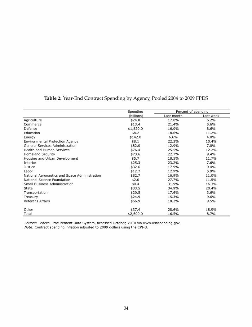
Table 2: Year-End Contract Spending by Agency, Pooled 2004 to 2009 FPDS
Spending (billions) Last month Last week
Agriculture $24.8 17.0% 6.2%Commerce $13.4 21.4% 5.6%Defense $1,820.0 16.0% 8.6%Education $8.2 18.6% 11.2%Energy $142.0 6.6% 4.0%Environmental Protection Agency $8.1 22.3% 10.4%General Services Administration $82.0 12.9% 7.0%Health and Human Services $76.4 25.5% 12.2%Homeland Security $73.6 22.7% 9.4%Housing and Urban Development $5.7 18.5% 11.7%Interior $25.3 23.2% 7.6%Justice $32.6 17.9% 9.4%Labor $12.7 12.9% 5.9%National Aeronautics and Space Administration $82.7 16.9% 11.0%National Science Foundation $2.0 27.7% 11.5%Small Business Administration $0.4 31.9% 16.3%State $33.5 34.9% 20.4%Transportation $20.5 17.6% 3.6%Treasury $24.9 15.3% 9.6%Veterans Affairs $66.9 18.2% 9.5%
Other $37.4 28.6% 18.9%Total $2,600.0 16.5% 8.7%
Percent of spending
Source: Federal Procurement Data System, accessed October, 2010 via www.usaspending.gov.Note: Contract spending inflation adjusted to 2009 dollars using the CPI-U.
34

Table 3: Year-End Contract Spending By Selected Product or Service Code, Pooled 2004to 2009 FPDS
Spending(billions) Last month Last week
Construction-relatedConstruction of structures and facilities $136.0 40.9% 28.6%Maintenance, repair, or alteration of real property $72.5 34.8% 20.1%Architect and engineering services $32.8 26.1% 13.8%Installation of equipment $4.0 33.9% 20.4%Prefabricated structures and scaffolding $3.7 34.9% 18.4%
Furnishings and office equipmentFurniture $8.0 37.3% 18.4%Office supplies and devices $4.0 24.9% 16.6%Household and commercial furnishings and appliances $1.2 37.8% 20.7%Office machines, text processing systems and equipment $1.1 33.5% 17.0%
I.T. services and equipmentAutomatic data processing and telecom. services $145.0 21.0% 12.3%Automatic data processing equipment $53.7 29.2% 14.9%
ServicesProfessional, admin, and management support services $336.0 19.1% 9.9%Research and development $309.0 11.3% 5.3%Utilities and housekeeping services $73.7 15.6% 9.1%
OngoingFuels, lubricants, oils and waxes $72.7 13.2% 0.7%Medical services $68.8 4.9% 1.7%Chemicals and chemical products $6.2 3.3% 1.3%Tires and tubes $1.0 8.7% 2.7%Toiletries $0.3 12.2% 3.0%
Military weapons systemsAircraft and airframe structural components $141.0 5.7% 2.9%Ships, small craft, pontoons, and floating docks $48.5 7.5% 2.1%Guided missiles $38.0 8.1% 3.5%
Other $1,111.6 13.6% 6.8%Total $2,600.0 16.5% 8.7%
Percent of spending
Source: Federal Procurement Data System, accessed October, 2010 via www.usaspending.gov.Note: Contract spending in the last month and week of the fiscal year by selected 2-digit product or service code, inflation adjusted to 2009 dollars using the CPI-U. Categories jointly account for 57.2 percent of total spending.
35
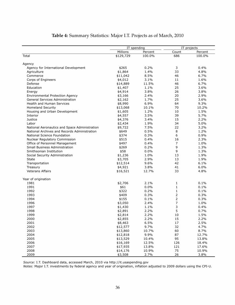
Table 4: Summary Statistics: Major I.T. Projects as of March, 2010
Millions Percent Count PercentTotal $129,729 100.0% 686 100.0%
AgencyAgency for International Development $265 0.2% 3 0.4%Agriculture $1,864 1.4% 33 4.8%Commerce $11,042 8.5% 46 6.7%Corps of Engineers $4,012 3.1% 11 1.6%Defense $14,889 11.5% 46 6.7%Education $1,407 1.1% 25 3.6%Energy $4,914 3.8% 26 3.8%Environmental Protection Agency $3,166 2.4% 20 2.9%General Services Administration $2,162 1.7% 25 3.6%Health and Human Services $8,990 6.9% 64 9.3%Homeland Security $13,068 10.1% 70 10.2%Housing and Urban Development $1,605 1.2% 10 1.5%Interior $4,557 3.5% 39 5.7%Justice $4,376 3.4% 15 2.2%Labor $2,434 1.9% 34 5.0%National Aeronautics and Space Administration $9,722 7.5% 22 3.2%National Archives and Records Administration $649 0.5% 8 1.2%National Science Foundation $374 0.3% 6 0.9%Nuclear Regulatory Commission $515 0.4% 16 2.3%Office of Personnel Management $497 0.4% 7 1.0%Small Business Administration $269 0.2% 9 1.3%Smithsonian Institution $58 0.0% 9 1.3%Social Security Administration $1,236 1.0% 13 1.9%State $3,705 2.9% 13 1.9%Transportation $12,514 9.6% 42 6.1%Treasury $4,921 3.8% 41 6.0%Veterans Affairs $16,521 12.7% 33 4.8%
Year of origination1981 $2,706 2.1% 1 0.1%1991 $61 0.0% 1 0.1%1992 $322 0.2% 1 0.1%1993 $409 0.3% 2 0.3%1994 $155 0.1% 2 0.3%1996 $3,050 2.4% 7 1.0%1997 $1,430 1.1% 3 0.4%1998 $2,891 2.2% 5 0.7%1999 $2,814 2.2% 10 1.5%2000 $2,855 2.2% 15 2.2%2001 $8,463 6.5% 17 2.5%2002 $12,577 9.7% 32 4.7%2003 $13,860 10.7% 60 8.7%2004 $12,818 9.9% 87 12.7%2005 $13,529 10.4% 95 13.8%2006 $16,169 12.5% 126 18.4%2007 $17,935 13.8% 121 17.6%2008 $14,176 10.9% 75 10.9%2009 $3,508 2.7% 26 3.8%
IT projectsIT spending
Source: I.T. Dashboard data, accessed March, 2010 via http://it.usaspending.govNotes: Major I.T. investments by federal agency and year of origination, inflation adjusted to 2009 dollars using the CPI-U.
36

Table 5: Summary Statistics: Quality Indexes and Project Characteristics for Major I.T.Projects
Mean Std. Dev. Min MaxPlanned cost (millions) 189.11 447.06 0.10 4770.89Overall rating 7.07 2.30 0.00 10.00
Rating subindexesCIO evaluation 3.95 0.94 1.00 5.00Cost rating 8.72 2.52 0.00 10.00Cost overrun 5.25 1.49 0.00 10.00Schedule rating 8.43 3.09 0.00 10.00
Count PercentInvestment phase
Full-Acquisition 59 8.6%Mixed Life Cycle 304 44.3%Multi-Agency Collaboration 29 4.2%Operations and Maintenance 278 40.5%Planning 16 2.3%
Service group Management of Government Resources 124 18.1%Missing 2 0.3%Service Types and Components 125 18.2%Services for Citizens 344 50.2%Support Delivery of Services to Citizen 91 13.3%
Line of businessAdministrative Management 15 2.2%Controls and Oversight 12 1.8%Defense and National Security 30 4.4%Disaster Management 20 2.9%Economic Development 9 1.3%Education 16 2.3%Energy 5 0.7%Environmental Management 32 4.7%Financial Management 81 11.8%General Government [CA] 45 6.6%General Science and Innovation 22 3.2%Health 55 8.0%Homeland Security 40 5.8%Human Resource Management 24 3.5%Income Security 17 2.5%Information and Technology Management 85 12.4%International Affairs and Commerce 7 1.0%Law Enforcement 12 1.8%Natural Resources 16 2.3%Planning and Budgeting 8 1.2%Public Affairs 13 1.9%Revenue Collection 8 1.2%Supply Chain Management 25 3.6%Transportation 45 6.6%Workforce Management 5 0.7%Other 39 5.7%
Total 686 100.0%
Source: I.T. Dashboard data, accessed March, 2010 via http://it.usaspending.govNotes: Planned total cost is inflation-adjusted to 2009 dollars using the CPI-U. Overall rating is a quality index that combines that CIO evaluation, cost rating, and scheduling rating subindexes (see text for details). It takes values from 0 to 10, with 10 being the best score. The CIO evaluation is the agency CIO's assessment of project quality. It takes values from 1 to 5, with 5 being the best. The cost rating is based on the absolute percent deviation between the planned and actual cost of the project. The cost overrun is a non-absolute measure that assigns over-cost projects the lowest scores. The schedule rating is based on the average tardiness of the project. The cost and schedule indexes takes values from 0 to 10, with 10 being the best. The line of business other category combines all categories with 4 or fewer projects.
37

Table 6: Ordered Logit Regressions of Overall Rating on Last Week and Controls
(1) (2) (3) (4)Last week 0.26 0.46 0.30 0.18
(0.07) (0.14) (0.10) (0.07)Year FE X X XAgency FE X XProject characteristics FE XN 671 671 671 671
Odds ratio of higher overall rating
Source: I.T. Dashboard data, accessed March, 2010 via http://it.usaspending.govNotes: Odds ratios from ordered logit regressions. Overall rating is a quality index that combines that CIO evaluation, cost rating, and scheduling rating subindexes (see text for details). It takes values from 0 to 10, with 10 being the best score. Project characteristics are fixed effects for investment phase, service group, and line of business (see Table 5). Observations weighted by inflation-adjusted spending. Standard errors in parentheses.
38

Tabl
e7:
Alt
erna
tive
Ove
rall
Rat
ings
Spec
ifica
tion
s
Contr
acts
< $
62M
Contr
acts
≥ $
62M
Unw
eighte
dW
inso
rize
d
wei
ghts
OLS
Hec
kman
se
lect
ion m
odel
(1)
(2)
(3)
(4)
(5)
(6)
Last
wee
k0.6
00.1
80.5
60.3
7-1
.00
-1.5
7(0
.23)
(0.1
1)
(0.1
4)
(0.1
2)
(0.3
9)
(0.6
4)
Year
FE
XX
XX
XAgen
cy F
EX
XX
XX
XPr
oje
ct c
har
acte
rist
ics
XX
XX
XX
Wei
ghte
d b
y sp
endin
gX
XX
XX
!-0
.87
(0.8
5)
R-s
quar
ed0.6
9N
335
336
671
671
671
3,8
03
Odds
ratio o
f hig
her
ove
rall
rating fro
m o
rder
ed logit
Coef
fici
ents
fro
m lin
ear
model
Sourc
e: I
.T.
Das
hboar
d d
ata,
acc
esse
d M
arch
, 2010 v
ia h
ttp:/
/it.
usa
spen
din
g.g
ov a
nd 2
003 t
o 2
010 E
xhib
it 5
3 r
eport
s, a
vaila
ble
at
htt
p:/
/ww
w.w
hiteh
ouse
.gov
/om
b/e
-gov
/docs
/.N
ote
s: C
olu
mns
(1)
to (
4)
show
odds
ratios
from
ord
ered
logit r
egre
ssio
ns.
Colu
mns
(1)
and (
2)
split
the
sam
ple
at
the
med
ian
valu
e. C
olu
mn (
3)
show
s odds
ratios
from
an u
nw
eighte
d r
egre
ssio
n.
Colu
mn (
4)
Win
sorize
s th
e sp
endin
g w
eight
at $
1 b
illio
n
(96th
per
centile
).Colu
mns
(5)
and (
6)
show
reg
ress
ion c
oef
fici
ents
fro
m lin
ear
regre
ssio
ns.
Colu
mn (
5)
report
s co
effici
ents
fro
m
a si
mple
OLS
reg
ress
ion.
Colu
mn (
6)
report
s co
effici
ent
from
a H
eckm
an s
elec
tion m
odel
with a
lin
ear
seco
nd s
tage.
In t
his
re
gre
ssio
n t
he
sam
ple
is
all m
ajor
I.T.
pro
ject
s re
cord
ed in t
he
Exh
ibit 5
3 r
eport
s. T
he
excl
uded
var
iable
in t
his
sel
ection m
odel
is
the
year
of pro
ject
origin
atio
n.
The
coef
fici
ent !
is t
he
implie
d c
oef
fici
ent
on t
he
inve
rse
Mill
's r
atio
sel
ection t
erm
. O
vera
ll ra
ting is
a qual
ity
index
that
com
bin
es t
hat
CIO
eva
luat
ion,
cost
rat
ing,
and s
ched
ulin
g r
atin
g s
ubin
dex
es (
see
text
for
det
ails
).
It t
akes
val
ues
fro
m 0
to 1
0,
with 1
0 b
eing t
he
bes
t sc
ore
. Pr
oje
ct c
har
acte
rist
ics
are
fixe
d e
ffec
ts for
inve
stm
ent
phas
e, s
ervi
ce
gro
up,
and lin
e of busi
nes
s (s
ee T
able
5).
Obse
rvat
ions
wei
ghte
d b
y in
flat
ion-a
dju
sted
spen
din
g u
nle
ss o
ther
wis
e m
entioned
. Robust
sta
ndar
d e
rrors
in p
aren
thes
es.
39

Table 8: Difference-in-Differences Estimates of Overall Rating on Justice and Last Week
(1) (2) (3) (4) (5) (6)Justice X last week 3.54 2.29 2.85 2.36 2.251 2.49
(1.19) (1.16) (0.75) (0.65) 0.593 0.898Last week -1.91 -1.06 -0.93 -0.99 -0.814 -0.468
(1.10) (0.82) (0.48) (0.39) 0.391 0.238Justice 0.06 -0.59 -3.33 -3.88 -4.022 -2.028
(0.51) (0.49) (0.47) (0.59) 0.578 1.01Year FE X X X X XAgency FE X X X XProject characteristics X X XWeighted by spending X X X X Winsorized*R-squared 0.06 0.22 0.58 0.68 0.60 0.48N 686 686 686 686 686 686
OLS Estimates
Source: I.T. Dashboard data, accessed March, 2010 via http://it.usaspending.govNotes: Coefficients from OLS regressions of overall rating on fully interacted Justice and last week indicators and controls. Overall rating is a quality index that combines that CIO evaluation, cost rating, and scheduling rating subindexes (see text for details). It takes values from 0 to 10, with 10 being the best score. Project characteristics are fixed effects for investment phase, service group, and line of business (see Table 5). Robust standard errors in parentheses. *Spending weight Winsorized at $1 billion (96th percentile).
40

Table A1: First Week Contract Spending for Selected Product or Service Codes, Pooled2004 to 2009 FPDS
Spending First week (billions) (percent)
LeasesLease or rental of facilities $29.2 26.2%Lease or rental of equipment $5.4 13.1%
Service contractsUtilities and housekeeping services $73.7 11.1%Medical services $68.8 11.3%Transportation, travel and relocation services $39.3 15.5%Social services $5.5 9.3%
Other $2,378.1 3.1%Total $2,600.0 4.0%
Source: Federal Procurement Data System, accessed October, 2010 via www.usaspending.govNote: Percent of contract spending in the last month and week of the fiscal year by selected 2-digit product or service code, inflation adjusted to 2009 dollars using the CPI-U. Categories account for about 8.5% of spending but 29.7% of first week spending.
41

Table A2: Ordered Logit Regressions of Subindexes on Last Week and Controls
Cost rating
Cost overrun
Schedule rating
(1) (2) (3) (4) (5)Last week of September 0.14 0.16 0.80 0.74 1.15
(0.06) (0.07) (0.36) (0.30) (0.66)Cost and schedule rating XAgency FE X X X X XYear FE X X X X XProject characteristics X X X X XWeighted by spending X X X X XN 671 671 671 671 671
Evalutation by Agency CIO
Odds ratio from ordered logit
Source: I.T. Dashboard data, accessed March, 2010 via http://it.usaspending.govNotes: Odds ratios from ordered logit regressions. The CIO evaluation is the agency CIO's assessment of project quality. It takes values from 1 to 5, with 5 being the best. The cost rating is based on the absolute percent deviation between the planned and actual cost of the project. The cost overrun is a non-absolute measure that assigns over-cost projects the lowest scores. The schedule rating is based on the average tardiness of the project. The cost and schedule indexes takes values from 0 to 10, with 10 being the best. Project characteristics are fixed effects for investment phase, service group, and line of business (see Table 5). Standard errors in parentheses.
42

Tabl
eA
3:Ye
ar-E
ndC
ontr
actC
hara
cter
isti
csR
egre
ssio
ns
Non-c
om
pet
itiv
eO
ne
bid
Non-c
om
pet
itiv
e or
one
bid
Cost
-re
imburs
emen
t T&
M/L
H
Cost
-re
imburs
emen
t or
T&
M/L
H(1
)(2
)(3
)(4
)(5
)(6
)La
st w
eek
-0.0
02
0.0
17
0.0
10
-0.0
32
0.0
04
-0.0
28
(0.0
02)
(0.0
02)
(0.0
02)
(0.0
02)
(0.0
01)
(0.0
02)
Year
FE
XX
XX
XX
Agen
cy F
EX
XX
XX
XPr
oduct
or
serv
ice
code
FEX
XX
XX
XR-s
quar
ed0.4
10.3
10.3
00.5
20.2
10.5
1N
402,4
00
402,4
00
402,4
00
402,4
00
402,4
00
402,4
00
Mea
n o
f dep
enden
t va
riab
le28.7
%20.0
%48.7
%30.0
%5.5
%35.5
%
Dep
enden
t Var
iable
:
Sourc
e: F
eder
al P
rocu
rem
ent
Dat
a Sys
tem
, ac
cess
ed O
ctober
, 2010 v
ia w
ww
.usa
spen
din
g.g
ovN
ote
: Ta
ble
show
s co
effici
ents
fro
m lin
ear
pro
bab
ility
model
reg
ress
ions
of co
ntr
act
type
and c
om
pet
itio
n t
ype
indic
ators
on las
t w
eek
and c
ontr
ols
. To
fac
ility
the
anal
ysis
, th
e dat
a is
aggre
gat
ed t
o t
he
leve
l of th
e co
variat
es a
nd t
he
regre
ssio
ns
are
wei
ghte
d b
y in
flat
ion-a
dju
sted
spen
din
g in e
ach c
ell.
43
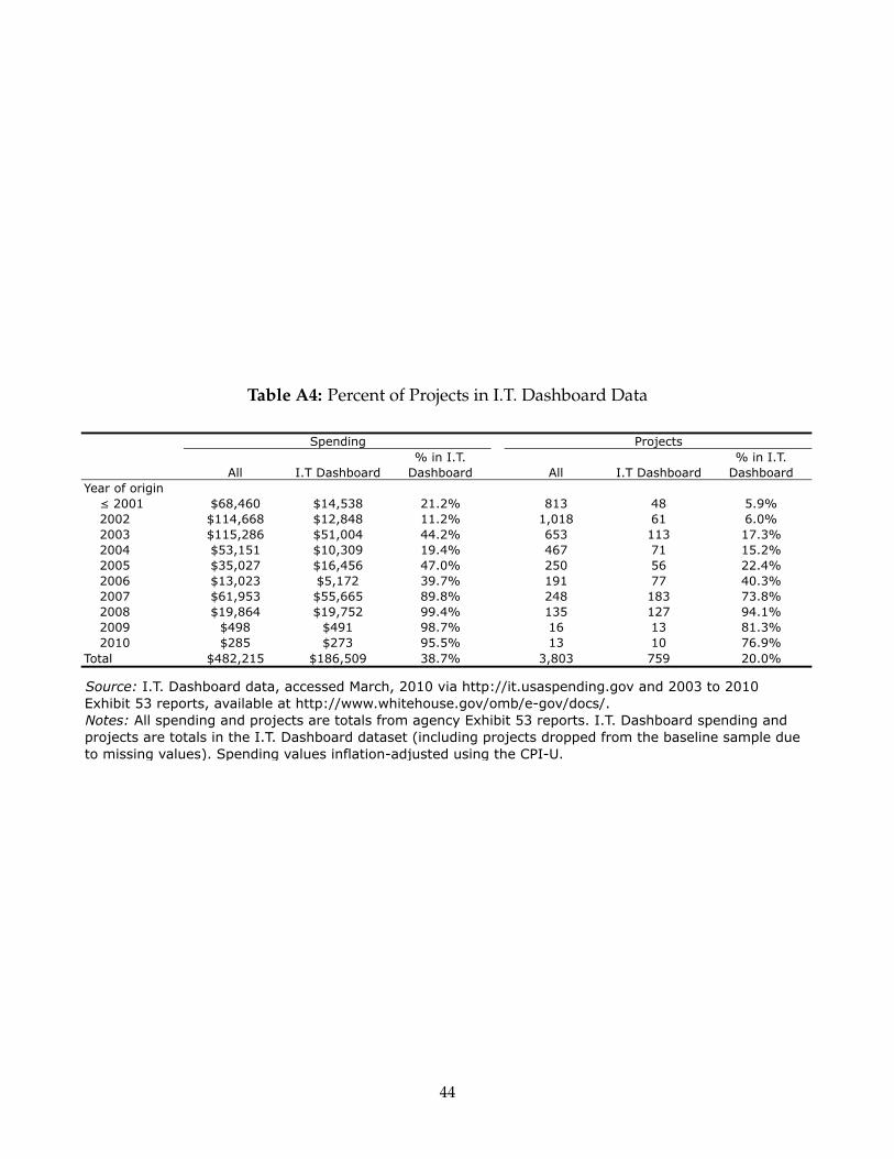
Table A4: Percent of Projects in I.T. Dashboard Data
All I.T Dashboard% in I.T.
Dashboard All I.T Dashboard% in I.T.
DashboardYear of origin≤ 2001 $68,460 $14,538 21.2% 813 48 5.9%2002 $114,668 $12,848 11.2% 1,018 61 6.0%2003 $115,286 $51,004 44.2% 653 113 17.3%2004 $53,151 $10,309 19.4% 467 71 15.2%2005 $35,027 $16,456 47.0% 250 56 22.4%2006 $13,023 $5,172 39.7% 191 77 40.3%2007 $61,953 $55,665 89.8% 248 183 73.8%2008 $19,864 $19,752 99.4% 135 127 94.1%2009 $498 $491 98.7% 16 13 81.3%2010 $285 $273 95.5% 13 10 76.9%
Total $482,215 $186,509 38.7% 3,803 759 20.0%
Spending Projects
Source: I.T. Dashboard data, accessed March, 2010 via http://it.usaspending.gov and 2003 to 2010 Exhibit 53 reports, available at http://www.whitehouse.gov/omb/e-gov/docs/.Notes: All spending and projects are totals from agency Exhibit 53 reports. I.T. Dashboard spending and projects are totals in the I.T. Dashboard dataset (including projects dropped from the baseline sample due to missing values). Spending values inflation-adjusted using the CPI-U.
44


