DIGITAL FILTER DESIGN FOR
AUDIO PROCESSING
Ethan Elenberg [email protected]
Stephanie Ng
Anthony Hsu [email protected]
Alaap Parikh
Marc L’Heureux [email protected]
E.J. Thiele
Michelle Yu [email protected]

Digital Filter Design for Audio Processing
Page 1 of 30
ABSTRACT
The goal of this research project was to
delve into digital signal processing with audio
files by learning the basics and then applying
them to the two specific areas of equalization
and delay/reverberation. Through the use of the
engineering mathematics program MATLAB, it
was possible to digitally create, apply, and
analyze these effects. Original sound files were
compared with their modified versions and the
respective graphs were used to determine the
effects of the filters, as well as the optimal
parameters for the best filters.
INTRODUCTION
Digital signal processing is the use of
computer (or, more generally, digital) algorithms
to alter a stream of data, and thus the
information being represented by the stream. It
is the extension of analog signal processing into
the digital realm.
The uses of digital signal processing are
many-fold in a modern, computer-driven society.
Filters may be used to scrub audio data streams
to increase the reliability of RADAR for defense
systems. They may also be used to “boost” and
“cut” specific frequency ranges in an audio file to
make it more pleasant to the ear. Even the
echoes and reverberations heard in many
popular songs are the products of post-recording
digital signal processing. Digital signal
processing is not only restricted to audio. It may
be used to remove noise from digital pictures
and television images.
We used MATLAB to design and
implement digital audio filters on sound files we
created.
BACKGROUND INFORMATION
MATLAB
MATLAB is an engineering mathematics
program. Unlike other similar programs, such as
Mathematica, MATLAB is focused more on
numerical computation than on algebraic
analysis. This makes it much more suited for
manipulating data than other programs.
MATLAB also offers a variety of
functions for analyzing and manipulating large
collections of data (which is what a digital signal
amounts to on a computer). Using the built-in
functions of the MATLAB programming
language and several functions provided by
Professor Orfanadis of the Rutgers University
Electrical and Computer Engineering
Department, it was much easier to design and
implement our digital filters than if we had
programmed them in another language, such as
C or Java. (1)
ANALOG VERSUS DIGITAL
As said before, digital signal processing
may be thought of as the extension of the ideas
and techniques of analog signal processing into
the digital realm.
Analog signals are representations of
streams of data in a medium that is continuously
variable with time. Stated differently, these
streams of data may represent different values
at different times, with an arbitrarily small
(practically non-existent) amount of time
between different values. These signals are
usually electric, and the data is represented by
some variable electric quantity (most usually
voltage). They are processed by changing the
pre-chosen quantity as prescribed by some
algorithm.
Digital signals are representations of
analog signals using discrete points of data with
some amount of time between them where the

Digital Filter Design for Audio Processing
Page 2 of 30
values may not change. The accuracy of the
digital representation of an analog signal can be
increased by decreasing the amount of time
between data points. Each data point is called a
sample; by increasing the number of samples
per second, one may increase the fidelity of the
digital stream. Digital streams are processed by
changing the individual samples, as prescribed
by some pre-chosen algorithm. (2)
DIGITAL FREQUENCIES
A stream is said to have a sampling
frequency, fs, if there are fs samples per second.
Changing the fs of a stream during playback will
change the perceived natural frequencies of the
stream. An audio CD normally has a sampling
frequency of 44,100 samples per second. The
digital frequency, fd, is equal to 𝑓1
𝑓𝑠
for some
natural (continuous) frequency, f1. Since time
has no meaning in a completely digital (discrete)
system, “samples” are used instead. fd is,
therefore, the digital analog of f1. The Nyquist
interval is the minimum number of samples per
second required to accurately represent an
analog signal of a given maximum frequency,
fmax. It is mathematically equal to 2*fmax. This is
the reason that most audio CDs have a
sampling frequency of 44,100 Hertz (Hz), or
samples per second; the approximate upper
bound of human hearing is about 20,000 Hz, or
approximately one-half of 44,100 Hz.
Most digital frequencies are also
expressed as radial frequencies, meaning they
have units of radians per cycle. To convert from
a natural frequency, f1, to radial frequency, fR,
one uses the equation fR = 2πf1. (2)
Figure 1: Frequency Chart (1)
FOURIER TRANSFORMS
A Fourier transform does for sound what
a prism does for light; it breaks it up into its
parts. Just as a beam of light is made up of
many different colors, a segment of sound is
made up of many different frequencies.
CONTINUOUS TIME FOURIER
TRANSFORM (CTFT)
A Fourier transform is a linear operator
that converts a function into a continuous
function of its frequency components. The
Fourier transform is mathematically written as
𝑋 𝑓 = 𝑥 𝑡 𝑒−𝑖2𝜋𝑓𝑡 𝑑𝑡∞
−∞
where
𝑡: 𝑡𝑖𝑚𝑒 𝑠𝑒𝑐𝑜𝑛𝑑𝑠

Digital Filter Design for Audio Processing
Page 3 of 30
𝑓: 𝑓𝑟𝑒𝑞𝑢𝑒𝑛𝑐𝑦 (𝐻𝑧)
𝑋: 𝑐𝑜𝑚𝑝𝑙𝑒𝑥 −
𝑣𝑎𝑙𝑢𝑒 𝑓𝑢𝑛𝑐𝑡𝑖𝑜𝑛 𝑡𝑎𝑡 𝑖𝑠 𝑥 𝑖𝑛 𝑡𝑒 𝑓𝑟𝑒𝑞𝑢𝑒𝑛𝑐𝑦
𝑑𝑜𝑚𝑎𝑖𝑛
Explained in more general terms, an
audio signal can be described as the summation
of sine functions, each with its own frequency
and amplitude. A Fourier transform converts the
signal into a continuous function with frequency f
and amplitude x(f). Fundamentally, if you pass a
given frequency to the function x(f), it will output
the magnitude of that frequency in the sound
sample.
DISCRETE TIME FOURIER
TRANSFORMS (DTFT)
A functional problem with the CTFT is
that it requires a continuous function as an input.
In real-world implementations, continuous
functions are impossible to obtain. Instead,
discrete time samples are used. This requires
the use of a function that can use a discrete time
function as an input. This function is the DTFT.
Mathematically, it is a special case of the
bilateral Z-transform where the Z-transform is
evaluated around the unit circle in the complex
domain. The bilateral Z-transform is defined as
𝑋 𝑧 = 𝑥 𝑛 𝑧−𝑛∞
−∞
.
The special case is when 𝑧 = 𝑒𝑖𝜔 , in which case
the DTFT becomes
𝑋 𝜔 = 𝑥 𝑛 𝑒−𝑖𝜔𝑛∞
𝑛=−∞
where
𝑛 𝑥 = 𝑇 ∗ 𝑥(𝑛𝑇)
𝜔 = 2𝜋𝑓𝑇 = 2𝜋 𝑓
𝑓𝑠 .
FINITE-LENGTH DTFT
One major problem with the DTFT is
that it evaluates the summation from negative
infinity to positive infinity. This, due to the fact
that computers have a finite amount of memory,
is impossible to evaluate on a computer. It is
thus modified to the approximation
𝑋 𝑤 = 𝑥 𝑛 𝑒−𝑖𝜔𝑛𝐿−1
𝑛=0
where
𝐿:𝑚𝑜𝑑𝑖𝑓𝑖𝑒𝑑 𝑠𝑒𝑞𝑢𝑒𝑛𝑐𝑒 𝑙𝑒𝑛𝑔𝑡.
As L increases, the difference between the finite
length DTFT and the unmodified sequence
decreases.
In practice, 𝑋(𝑤) is evaluated a finite
number of times, n, over one period, 2π. Thus,
𝜔𝑘 =2𝜋
𝑁𝐾, 𝑓𝑜𝑟 𝐾 = 0,1,2… ,𝑁 − 1
.
When you substitute 𝜔𝐾 into 𝑋(𝑤), you get the
following equation:
𝑋 𝐾 = 𝑥[𝑛]𝑒−𝑖2𝜋𝐾𝑁𝑛
𝐿−1
𝑛=0
.

Digital Filter Design for Audio Processing
Page 4 of 30
Because 𝑥 𝑛 = 0 for 𝑛 ≥ 𝐿, if 𝑛 ≥ 𝐿, the
equation becomes:
𝑋 𝐾 = 𝑥[𝑛]𝑒−𝑖2𝜋𝑘𝑁𝑛
𝑁−1
𝑛=0
.
In this format, X[K] is now a discrete Fourier
transform (DFT). In this format, N is the
resolution at which the DTFT is sampled and L
is the limit of the resolution of the DTFT. Thus, it
makes sense for N and L to be very close to
each other. N and L are almost always selected
so that N ≥ L.
Obtaining a DFT is important because a
DFT is both discrete and finite, meaning that it
can easily be processed by a computer.
FAST FOURIER TRANSFORMS (FFT)
An FFT is a method of evaluating a DFT
on a computer system. If you were to directly
evaluate the DFT function,
𝑋[𝑛] = 𝑥[𝑛]𝑒−2𝜋𝑖𝑁 𝑛𝑘
𝐿−1
𝑛=0
,
it would take a time of 𝑂(𝑁2). If an FFT is used,
this is reduced to a time of 𝑂(𝑁 log𝑁). This
means that on a sample of 1,024 bits, the FFT is
102.4 times faster then directly computing the
DFT (2). Without the use of FFTs, Fourier
transforms would be impractical for most
applications. The most common FFT is the
Cooley-Turkey algorithm. Other FFT algorithms
include Prime-factor FFT algorithm, Bruun's FFT
algorithm, Rader's FFT algorithm, and
Bluestein's FFT algorithm.
MATLAB SPECTRUM FUNCTION
Spectrum is a function we used frequently in
MATLAB to look at the spectral envelope of a
recorded sine wave. Spectrum takes in a vector
of numbers from a .wav file and the sampling
frequency of the file. The function outputs the
FFT of the .wav file in a graph. Figure 1 is what
a sample of the raw plot of a 440 Hz sine wave
looks like.
Figure 2
The following example outputs the FFT of the
440 Hz sine wave.
>>[x,fs]=wavread(‘440hzsine.wav’);
>>spectrum(x,fs);

Digital Filter Design for Audio Processing
Page 5 of 30
This code outputs the graph shown in Figure 3.
Figure 3
Because the input contains only one
frequency at 440Hz, the output FFT has one
sharp spike at the 440Hz position. An input with
only one frequency never happens in practical
applications.
The next example is a more common
sound, the human voice. This is what a sample
of the raw plot of our voice sample looks like:
Figure 4
The following MATLAB code shows the FFT of
the voice sample.
>>[x,fs]=wavread(‘vocals2.wav’);
>>spectrum(x,fs);
This sample demonstrates the utility of
the FFT because it contains many frequencies
with different amplitudes, which would be very
difficult to see with only the raw plot.
Figure 5
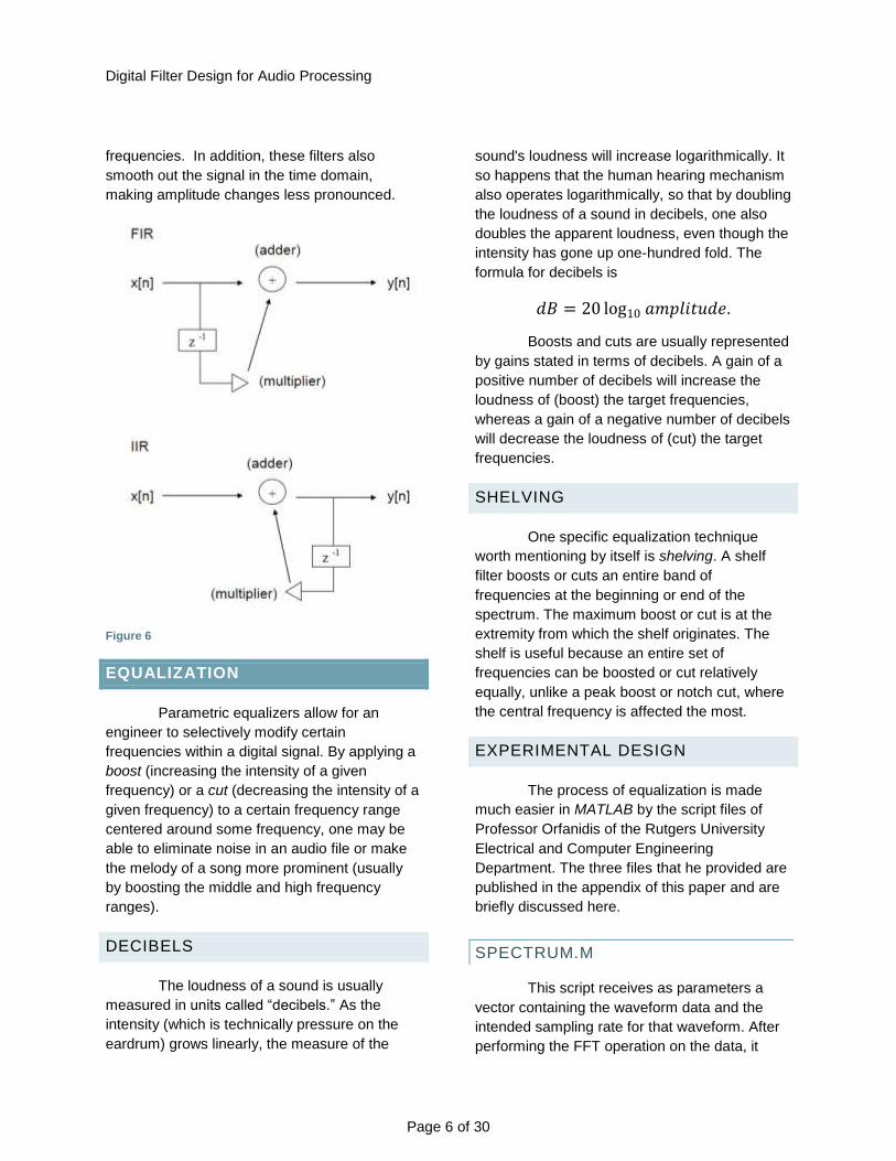
FIR AND IIR FILTERS
Filters are electronic circuits that
respond to impulses, processing signals by
enhancing certain aspects and/or reducing
certain aspects. There are several different
types of filters. A finite impulse response (FIR)
filter is one in which the output signal goes to
zero in some finite amount of time. In contrast,
an infinite impulse response (IIR) filter may run
for an arbitrarily long period of time and never
have the output go to zero. The difference
between the two types of filters is that an IIR
filter is recursive; i.e., an IIR filter will take its
previous output and use it as input for the next
output, whereas an FIR filter will take as input
the current sample in addition to some previous
sample. In other words, an IIR filter has internal
feedback while an FIR filter does not. Figure 6
shows an example of block diagrams for an FIR
filter and an IIR filter.
Some common FIR and IIR filters
include low-pass and high-pass filters, which cut
back high and low frequencies, while passing
low and high frequencies, respectively (hence
their names), while amplifying the passed
Digital Filter Design for Audio Processing
Page 6 of 30
frequencies. In addition, these filters also
smooth out the signal in the time domain,
making amplitude changes less pronounced.
Figure 6
EQUALIZATION
Parametric equalizers allow for an
engineer to selectively modify certain
frequencies within a digital signal. By applying a
boost (increasing the intensity of a given
frequency) or a cut (decreasing the intensity of a
given frequency) to a certain frequency range
centered around some frequency, one may be
able to eliminate noise in an audio file or make
the melody of a song more prominent (usually
by boosting the middle and high frequency
ranges).
DECIBELS
The loudness of a sound is usually
measured in units called “decibels.” As the
intensity (which is technically pressure on the
eardrum) grows linearly, the measure of the
sound's loudness will increase logarithmically. It
so happens that the human hearing mechanism
also operates logarithmically, so that by doubling
the loudness of a sound in decibels, one also
doubles the apparent loudness, even though the
intensity has gone up one-hundred fold. The
formula for decibels is
𝑑𝐵 = 20 log10 𝑎𝑚𝑝𝑙𝑖𝑡𝑢𝑑𝑒.
Boosts and cuts are usually represented
by gains stated in terms of decibels. A gain of a
positive number of decibels will increase the
loudness of (boost) the target frequencies,
whereas a gain of a negative number of decibels
will decrease the loudness of (cut) the target
frequencies.
SHELVING
One specific equalization technique
worth mentioning by itself is shelving. A shelf
filter boosts or cuts an entire band of
frequencies at the beginning or end of the
spectrum. The maximum boost or cut is at the
extremity from which the shelf originates. The
shelf is useful because an entire set of
frequencies can be boosted or cut relatively
equally, unlike a peak boost or notch cut, where
the central frequency is affected the most.
EXPERIMENTAL DESIGN
The process of equalization is made
much easier in MATLAB by the script files of
Professor Orfanidis of the Rutgers University
Electrical and Computer Engineering
Department. The three files that he provided are
published in the appendix of this paper and are
briefly discussed here.
SPECTRUM.M
This script receives as parameters a
vector containing the waveform data and the
intended sampling rate for that waveform. After
performing the FFT operation on the data, it

Digital Filter Design for Audio Processing
Page 7 of 30
outputs a graph showing the spectral envelope
of the waveform. spectrum is especially useful
for determining which cuts and boosts to apply
to a stream and for reviewing the results of a cut
or boost after application.
MAGRESPONSE.M
This script receives as parameters two
vectors – a and b – which contain the
coefficients for descending powers of z for the
denominator and numerator (respectively) of the
transfer function 𝐻(𝑧). It then plots them as
though the unit impulse were filtered using the
transfer function and displays that graph. This
script is useful for determining the overall
behavior of a specific cut or boost, or that of all
of the cascaded cuts and boosts in the final
filter.
PARMEQ.M
This script takes as parameters three
gain values (all in magnitude gain, not decibels)
and two frequency values (in radians per
sample). parmeq returns a matrix that contains
two vectors – a and b – which contain the
coefficients for descending powers of z for the
denominator and numerator (respectively) of the
transfer function for the filter specified by the
parameters of the script.
The first gain value, G0, specifies which
value to cut or boost from. For the purposes of
this paper, G0 will remain 1, meaning that there
is a net change on the signal of 0 dB or, more
simply, there is no net change on the signal. The
next parameter, G, specifies what amount of
gain to apply to the frequency band specified
later. The third gain parameter, GB, specifies the
amount of gain to be applied at the edges of the
bandwidth. For all non-shelf filters created in this
paper, a constant of 1/ 2 is used, and for
shelved filters, the bandwidth gain in decibels
applied is equal to one half of the gain of the
boost or cut.
The two frequency values specify the
band of frequencies to which the filter will be
applied. The first, w0, is the center frequency of
the boost or cut. The second, dw, specifies one-
half of the bandwidth of the filter.
GUITARDISTORT.M
The first of two parametric equalization
filters we created is defined in a script called
guitarDistort. The filter operates on an audio
signal represented in the file guitarDistort.wav.

Digital Filter Design for Audio Processing
Page 8 of 30
The raw signal (represented in the
middle graph of figure 7) has a heavily saturated
bass within the frequency band of approximately
80 Hz to 200 Hz. The band also has peak
magnitudes that rival those of the frequencies in
the middle band, where most of the melody
comes from. The saturation of this band is
probably due to the white (random) noise that
was overlaid onto the signal of the guitar during
recording, which means that we can cut the
bass slightly. At the same time, the bass
frequencies offer both character and melody to
the sound that the signal represents, and
cannot, therefore, be completely removed from
the signal. To correct for the prominence of the
bass frequencies, we applied a 12 dB cut
centered at 150 Hz to this band, which removes
a good deal of muddiness from the final signal.
Upon applying the bass-cut filter, we
realized that the middle frequencies (which have
peaks in the range of approximately 200 Hz to
600 Hz) now seemed overbearing. The only
option was to cut these as well, since restoring
the bass to its original intensity would cause the
sound to once again become muddy. We
decided to design the cut such that the target
frequencies would remain more intense (in
terms of decibels) than the bass frequencies, but
so that they would be cut to the same “intensity”
range as the other bands of frequencies. The cut
applied is 4.5 dB, centered at 300 Hz.
We finally noticed that the distortion
effect was not as full as it should be, due to the
filtering we applied. To correct this, we applied a
6.8 dB boost with a bandwidth of 2,000 Hz
centered at 2,500 Hz to amplify the white noise
in that region. The band chosen was selected
specifically so that the boost would neither affect
any of the areas of melody nor amplify any of
the very high audible frequencies, which would
result in a very distracting, high-pitched sound in
the final audio representation.
PIANOMARIO.M
Our second parametric equalizer is
defined in a script called pianoMario. The filter
operates on an audio signal represented in the
file pianoMario.wav.
Similar to the guitarDistort filter, we
recognized the bass frequencies to be slightly
overbearing. We also noticed from the spectral
envelope graph that there were some low-
intensity, low-frequency disturbances. To fix
both of these problems, we applied a low-shelf
filter with a bandwidth of 220 Hz and a
magnitude of 3 dB.
Figure 7: “guitardistort.wav” (top to bottom) magnitude response of the filter, spectrum of input, spectrum of output

Digital Filter Design for Audio Processing
Page 9 of 30
We also found a narrow band of
frequencies between approximately 250 Hz and
350 Hz that were much more intense than those
that surrounded them. We applied a 5 dB cut
centered at 300 Hz with a bandwidth of 90 Hz to
reduce the intensity of this band so that the
middle tones would sound evenly loud.
DELAY AND REVERBERATION
DELAY
The effect of delay is achieved when a
signal is played and then a modified version of
that signal is played back after a period of time,
either one time or multiple times, resulting in an
echoing effect. The simplest version of delay is
an FIR filter through which a signal is played
back only one time. This is called simple delay.
Delay time and relative amplitude (and hence
relative intensity) for the echo are two
parameters that can be specified.
REVERBERATION
Reverberation, or reverb, is a slightly
more complex IIR form of delay. Reverb is used
to digitally simulate a surrounding by modeling
echoes that would naturally be present in that
environment. The simplest type of reverb is the
plain reverb, which is essentially just a simple
delay in an IIR form. In this form, part of the
echo output is re-inputted into the system every
delay period. In each iteration, the preceding
delayed output is multiplied by the multiplier
coefficient. It is important that the multiplier
coefficient is less than one, or else the
reverberations will grow increasingly louder.
With a coefficient less than one, the
reverberations decay exponentially and
approach zero.
UNIT IMPULSES AND IMPULSE
FUNCTIONS
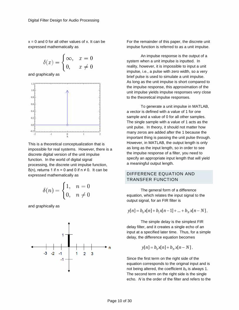
A unit impulse is a pulse with no width
that still maintains an area of unity, i.e., 1. This
causes the amplitude to be infinite. The unit
impulse function, δ(x), is defined to be infinity at
Figure 8: “panomario.wav” (top to bottom) magnitude response of the filter, spectrum of input, spectrum of output
Digital Filter Design for Audio Processing
Page 10 of 30
x = 0 and 0 for all other values of x. It can be
expressed mathematically as
and graphically as
This is a theoretical conceptualization that is
impossible for real systems. However, there is a
discrete digital version of the unit impulse
function. In the world of digital signal
processing, the discrete unit impulse function,
δ(n), returns 1 if n = 0 and 0 if n ≠ 0. It can be
expressed mathematically as
and graphically as
For the remainder of this paper, the discrete unit
impulse function is referred to as a unit impulse.
An impulse response is the output of a
system when a unit impulse is inputted. In
reality, however, it is impossible to input a unit
impulse, i.e., a pulse with zero width, so a very
brief pulse is used to simulate a unit impulse.
As long as the unit impulse is short compared to
the impulse response, this approximation of the
unit impulse yields impulse responses very close
to the theoretical impulse responses.
To generate a unit impulse in MATLAB,
a vector is defined with a value of 1 for one
sample and a value of 0 for all other samples.
The single sample with a value of 1 acts as the
unit pulse. In theory, it should not matter how
many zeros are added after the 1 because the
important thing is passing the unit pulse through.
However, in MATLAB, the output length is only
as long as the input length, so in order to see
the impulse response of a filter, you need to
specify an appropriate input length that will yield
a meaningful output length.
DIFFERENCE EQUATION AND
TRANSFER FUNCTION
The general form of a difference
equation, which relates the input signal to the
output signal, for an FIR filter is
][...]1[][][ 10 Nnxbnxbnxbny N .
The simple delay is the simplest FIR
delay filter, and it creates a single echo of an
input at a specified later time. Thus, for a simple
delay, the difference equation becomes
][][][ 0 Nnxbnxbny N .
Since the first term on the right side of the
equation corresponds to the original input and is
not being altered, the coefficient b0 is always 1.
The second term on the right side is the single
echo. N is the order of the filter and refers to the

Digital Filter Design for Audio Processing
Page 11 of 30
time delay of the echo. Digitally, a time delay is
expressed in terms of samples. Thus, N is in
terms of samples. For a simple delay, b0 = 1, bN
is expressed as α, and N is referred to as the
delay D, which is, again, in units of samples.
The difference equation then becomes
)()()( Dnxnxny .
α is called the weighting factor, which is a
measure of the relative amplitude of the echo
compared to the input. For example, if α = 0.5,
the echo would have half the amplitude of the
input and would sound about half as loud.
The Z-transform is applied to the
difference equation to convert it from a time-
domain signal to a complex frequency-domain
representation. The application of the Z-
transform to the difference equation yields the
transfer function, which applies the desired
effect in the complex frequency-domain.
The general form of the transfer function
is
N
N
i
iN
i
z
zb
zH
0)( .
For a simple delay, this equation becomes
D
D
i
iD
i
z
zb
zH
0)( .
However, this can be simplified further: b0 = 1
and bD = α. For all other values of i, bi = 0.
Thus, the transfer function for a simple delay
becomes
D
D
DDD
zz
zzzH
11
)(0
.
In MATLAB, the function „simple.m‟ acts
as the difference equation and the
corresponding transfer function. It takes as
input a vector x, which could be a sound file,
along with a weighting factor α, a delay time Dt,
in seconds, which is easily converted to samples
D by multiplying Dt by the sampling frequency,
fs, which is the last input parameter. So in
summary, the function „simple.m‟ takes as input
(x, α, Dt, fs). The function outputs the filtered
result y, along with the filter coefficients a and b.
Supposing the input x were a sound file, the
output y would be the filtered sound with the
delay effect. a is a matrix of the filter coefficients
in the denominator of the transfer function, and b
is a matrix of the numerator filter coefficients in
the same function. As suggested by the general
form of a transfer function for a simple delay, a
is always 1 for a FIR simple delay filter. b is a 1
by D (which is equal to Dt × fs) matrix that has a
value of 1 for the first column, a value of a for
the Dth column, and a value of 0 for all other
columns.
The filter coefficients a and b can then
be passed through the function „imresponse.m,‟
which takes as input these filter coefficients
along with two more parameters, impulse length
and sampling frequency. This function outputs a
plot of the impulse response of the generated
filter, which in this case was a simple delay filter.
When dealing with IIR filters, such as
plain reverb filters, different versions of the
difference equation and transfer function are
used. The general form of the difference
equation is
][][][0 1
jnyainxbnyP
i
Q
j
ji
.
The first summation refers to feed-forward
filtering, where P is the feed-forward filter order
and the bi is the feed-forward filter coefficient.
The second summation refers to feedback
filtering, where Q is the feedback filter order and
Digital Filter Design for Audio Processing
Page 12 of 30
the aj is the feedback filter coefficient. x[n] is the
input signal and y[n] is the output signal. In our
case, for a plain reverb filter, we are not dealing
with feed-forward filtering, so P = 0. Thus, we
can simplify the general form of the difference
equation to
][][][1
0 jnyanxbnyQ
j
j
.
However, this can be simplified further. We are
only casting a single delay in IIR form, which we
specify to occur D samples later. D is equivalent
to Q, so D also represents the feedback filter
order. b0 = 1 because this coefficient
corresponds to the original input x[n], which we
are not altering. aD is usually represented by α,
which is called the weighting sample and is a
measure of the relative amplitude of the next
reverb compared to the previous one (or the
original sample if the next reverb is the first
reverb). All other aj coefficients have a value of
0 because we are only casting a single delay,
rather than multiple delays, in IIR form. The
simplest general form of the difference equation
of a plain reverb filter is thus
][][][ Dnynxny .
You will notice that the second term on the right
side of the equation is a function of y. This is
the previous output that is re-inputted, which
leads to the reverberation effect.
Now, to find our transfer function, we
again apply the Z-transform to the difference
equation. The general form of the transfer
function is
jQ
j
j
P
i
i
i
za
zb
zH
0
0)( .
Now recall that P = 0, b0 = 1, Q = D, and aj = 0
except for aD, which equals α. Then the transfer
function becomes
DzzH
1
1)( .
EXPERIMENTAL DESIGN
SIMPLE.M
In MATLAB, the function „simple.m‟ acts
as the difference equation and the
corresponding transfer function. It takes as
input a vector x, which could be a sound file,
along with a weighting factor α, a delay time Dt,
in seconds, which is easily converted to samples
D by multiplying Dt by the sampling frequency,
fs, which is the last input parameter. So in
summary, the function „simple.m‟ takes as input
(x, α, Dt, fs). The function outputs the filtered
result y, along with the filter coefficients a and b.
Supposing the input x were a sound file, the
output y would be the filtered sound with the
delay effect. a is a matrix of the filter coefficients
in the denominator of the transfer function, and b
is a matrix of the numerator filter coefficients in
the same function. As suggested by the general
form of a transfer function for a simple delay, a
is always 1 for a FIR simple delay filter. b is a 1
by D (which is equal to Dt × fs) matrix that has a
value of 1 for the first column, a value of a for
the Dth column, and a value of 0 for all other
columns.
For this project, we wrote a program
called simpledelay.m, which serves four
purposes. First, it takes a .wav file as input and
converts it to a vector of samples. Then, the
script runs simple.m using the two inputted
parameters, plays the modified signal, and
generates graphs of the impulse response,
original waveform, and output waveform.
Digital Filter Design for Audio Processing
Page 13 of 30
Figure 9
PLAIN.M
The MATLAB function „plain.m‟ applies
the difference equation and the transfer function.
It takes the same parameters as „simple.m‟ and
outputs the same things. The only difference is
that the filtered sound has a reverberation effect
applied and the filter coefficients a and b are
different. b, the numerator coefficient, is always
1, and a is a 1 × D matrix that has 1 as its first
column, α as its last column, and zeros for all
other columns.
Our program, called plaindelay.m, works
similarly to simpledelay.m; it imports a .wav file,
adds reverb using plain.m, plays the new signal,
and generates impulse, input, and output
graphs.
Figure 10
COMPLEXDELAY.M
To more accurately simulate natural
reverberation, we also designed a program
called complexdelay.m. This script takes as
input a .wav file and five sets of α factors and
delay times, corresponding to five plain reverb
effects. After converting the file to samples,
three plain reverbs are applied independently to
the original waveform. It sums the resulting
signals before performing two additional reverbs.
Figure 11
IMRESPONSE.M
Both the simple.m filter and the plain.m
filter output filter coefficients a and b. These
filter coefficients can then be passed through the
function „imresponse.m,‟ which takes as input
these filter coefficients along with two more
parameters, impulse length and sampling
frequency. This function then outputs a plot of
the impulse response of the generated filter.
GUITARARPEG.WAV
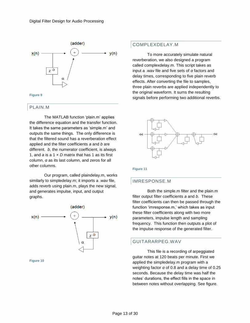
This file is a recording of arpeggiated
guitar notes at 120 beats per minute. First we
applied the simpledelay.m program with a
weighting factor α of 0.8 and a delay time of 0.25
seconds. Because the delay time was half the
notes‟ durations, the effect fills in the space in
between notes without overlapping. See figure.
Digital Filter Design for Audio Processing
Page 14 of 30
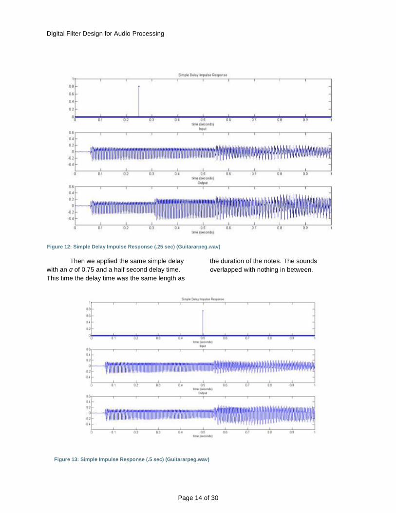
Then we applied the same simple delay
with an α of 0.75 and a half second delay time.
This time the delay time was the same length as
the duration of the notes. The sounds
overlapped with nothing in between.
Figure 12: Simple Delay Impulse Response (.25 sec) (Guitararpeg.wav)
Figure 13: Simple Impulse Response (.5 sec) (Guitararpeg.wav)
Digital Filter Design for Audio Processing
Page 15 of 30
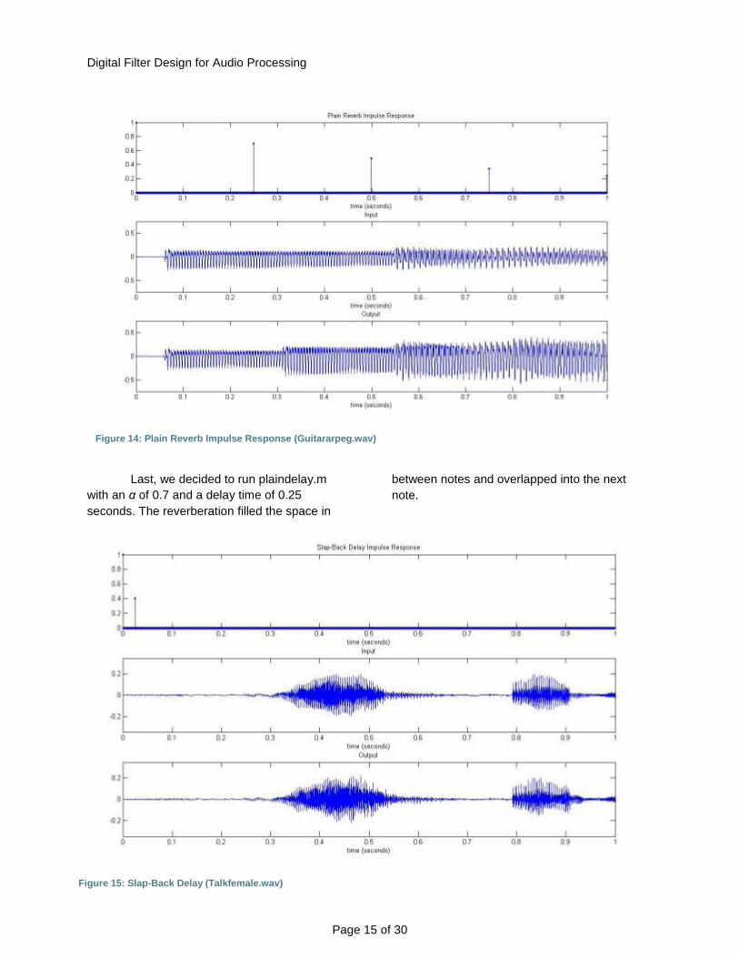
Last, we decided to run plaindelay.m
with an α of 0.7 and a delay time of 0.25
seconds. The reverberation filled the space in
between notes and overlapped into the next
note.
Figure 14: Plain Reverb Impulse Response (Guitararpeg.wav)
Figure 15: Slap-Back Delay (Talkfemale.wav)

Digital Filter Design for Audio Processing
Page 16 of 30
TALKFEMALE.WAV
This signal is one recorded paragraph of a
woman‟s voice. First, we set the weighting factor
to 0.5 and ran simpledelay.m with a 0.060
second delay time. This created a quick, simple
echo in which the original sound and the
delayed sound are still differentiable.(Figure 16)
Although the delay was quick, it was not
a true slap-back delay effect. By reducing the
delay time to 25 milliseconds and re-executing
the program, we created a delay that blended
with the original sound. The voice was almost
doubled on itself.(Figure 15)
Figure 16: Simple Delay Response (Talkfemale.wav)
Figure 17: Complex Reverb Response (Talkfemale.wav)

Digital Filter Design for Audio Processing
Page 17 of 30
Finally, we ran the complexdelay.m script with α1
= .4, dt1 = .14, α2 = .38, dt2 = .118, α3 = .42, dt3 =
0.094, α4 = .15, dt4 = 0.086, α = .35, and dt5 =
.073. The first three plain reverbs were applied
separately and then added together. Then, the
last two were applied in succession to the
already modified file. This complex reverb
simulates the natural echoing of a large room or
hall. (Figure 17)
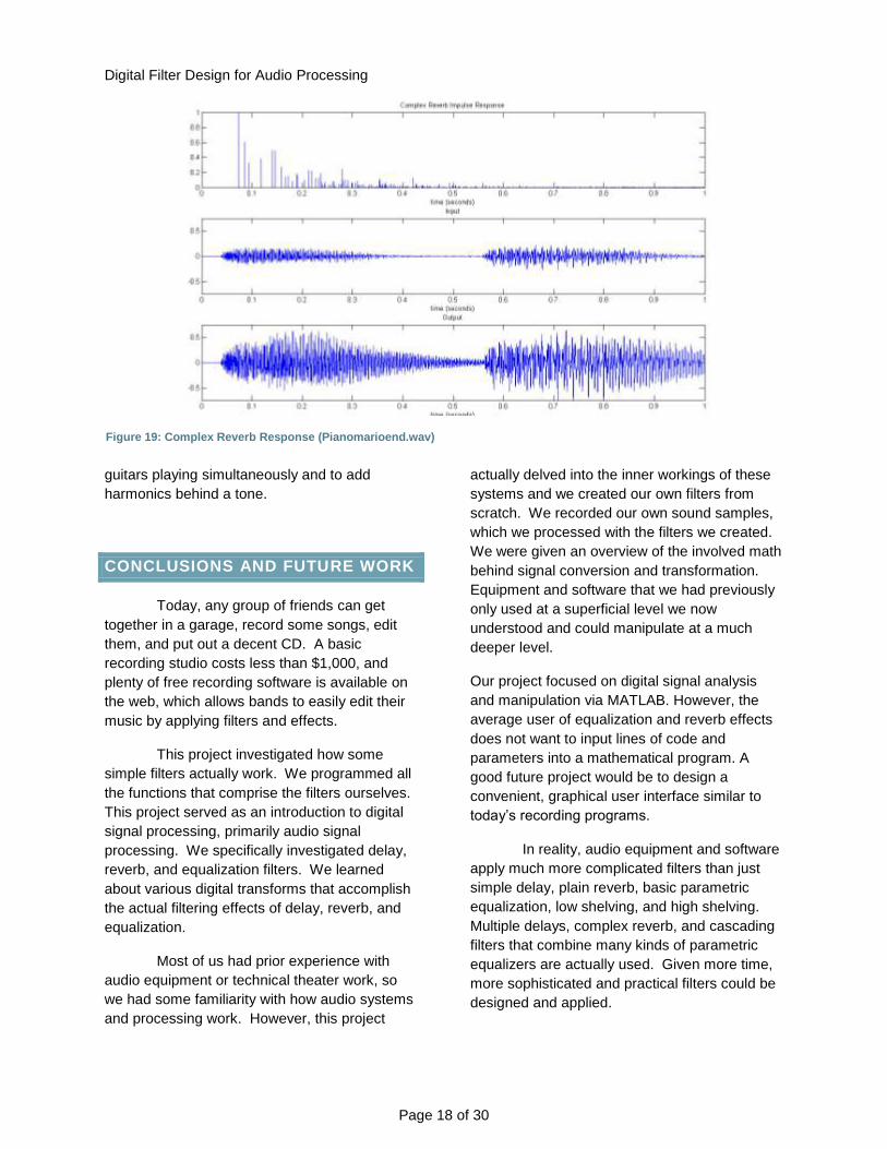
PIANOMARIOEND.WAV
This audio file is a short piano recording.
First, we ran plaindelay.m with an α of 0.67 and
a delay time of 0.089 seconds to add a plain
reverb effect. This quick effect simulated a slight
echo similar to that of a small room.
Then, we ran another complex reverb
with α1 = .5, dt1 = .14, α2 = .48,dt2 =.118, α3 = .52,
dt3 = .094, α4 = .25, dt4 = .086, α5 = .45, and dt5
= .073. This series of plain reverbs recreated the
environment of a large hall for a piano.
APPLICATIONS
A common application of a simple delay
filter is a „slap-back delay‟ effect. This filter
applies a very short delay (about 25
milliseconds), which is too close to the original
sample for the human ear to distinguish it as an
echo. Instead, we hear it as a richer, fuller
voice.
In practice, long delay times are
generally not used, since reverb should not
sound like distinct repetitions of the original
sample but should create an interesting effect
through a blend of multiple delays that creates a
dynamic texture. However, long delay times can
be used with arpeggiated guitar tracks with
substantial rests to give the effect of multiple
Figure 18: Plain Reverb Response (Panomarioend.wav)
Digital Filter Design for Audio Processing
Page 18 of 30
guitars playing simultaneously and to add
harmonics behind a tone.
CONCLUSIONS AND FUTURE WORK
Today, any group of friends can get
together in a garage, record some songs, edit
them, and put out a decent CD. A basic
recording studio costs less than $1,000, and
plenty of free recording software is available on
the web, which allows bands to easily edit their
music by applying filters and effects.
This project investigated how some
simple filters actually work. We programmed all
the functions that comprise the filters ourselves.
This project served as an introduction to digital
signal processing, primarily audio signal
processing. We specifically investigated delay,
reverb, and equalization filters. We learned
about various digital transforms that accomplish
the actual filtering effects of delay, reverb, and
equalization.
Most of us had prior experience with
audio equipment or technical theater work, so
we had some familiarity with how audio systems
and processing work. However, this project
actually delved into the inner workings of these
systems and we created our own filters from
scratch. We recorded our own sound samples,
which we processed with the filters we created.
We were given an overview of the involved math
behind signal conversion and transformation.
Equipment and software that we had previously
only used at a superficial level we now
understood and could manipulate at a much
deeper level.
Our project focused on digital signal analysis
and manipulation via MATLAB. However, the
average user of equalization and reverb effects
does not want to input lines of code and
parameters into a mathematical program. A
good future project would be to design a
convenient, graphical user interface similar to
today‟s recording programs.
In reality, audio equipment and software
apply much more complicated filters than just
simple delay, plain reverb, basic parametric
equalization, low shelving, and high shelving.
Multiple delays, complex reverb, and cascading
filters that combine many kinds of parametric
equalizers are actually used. Given more time,
more sophisticated and practical filters could be
designed and applied.
Figure 19: Complex Reverb Response (Pianomarioend.wav)

Digital Filter Design for Audio Processing
Page 19 of 30
Throughout the course of this project,
we created programs to perform multiple tasks.
Another topic of study could focus on using an
artificial-intelligence algorithm to analyze a given
waveform, detect imperfections, suggest filter
parameters, and apply them in one
implementation.
Finally, all the filtering done was
completely digitalized. If we were to extend this
project to incorporate live filtering, we would
have to work in the analog domain as well as the
field of analog to digital conversion. This would
require an introduction into the theory and
background of analog signal processing.
This project gave us a sample of the
huge world of signal processing. The
background behind it is very technical, but this
field has very clear real-world applications.
ACKNOWLEDGMENTS
We would first like to thank Rutgers, the
Governor's School of New Jersey, and all of the
Governor's School Staff and Organizers for
providing us with this great program and
research opportunity. We would also like to
thank Brian Maguire, our research mentor, for
generously lending us his time and experience
in teaching, helping, and pushing us along with
our research project. Also, we would like to
thank Blase Ur, the Governor's School program
coordinator, for his advice and suggestions as
well as his guidance on the project and paper,
and all of the great counselors for their
motivation and assistance throughout our stay at
Rutgers. Finally, we would like to thank all of our
parents and teachers for everything that they
have done for us throughout the years.
CITATIONS
1. Palm III, William J. Introduction to Matlab 7
for Engineers. New York : Mc Graw Hill, 2005. 0-
07-254818-5.
2. Rossing, Thomas D, Moore, Richard and
Wheeler, Paul A. The Science of Sound. New
York : Addison Wesley, 2002. 0-8053-8565-7.
3. Oppenheim, Alan V and Willsky, Alan S.
Signals & Systems. Upper Saddle River :
Prentice Hall, 1997. 0-13-814757-4.
4. IDCS. Frequency Chart. [Online] [Cited: July
16, 2007.]
http://www.idcs.info/images/frequency_chart_we
b.jpg.
5. Peters, Randall D. Graphical explanation for
the speed of the Fast Fourier Transform .
[Online] Febuary 18, 2003. [Cited: July 18,
2007.] http://arxiv.org/html/math.HO/0302212.

Digital Filter Design for Audio Processing
Page 20 of 30
APPENDIX A (MATLAB CODE)
SIMPLE.M
function [y,b,a]=simple(x,alpha,Dt,fs)
Dsamp=Dt*fs;
b=[1 zeros(1,Dsamp-2) alpha];
a=1;
y=filter(b,a,x);
PLAIN.M
function [y,b,a]=plain(x,alpha,Dt,fs)
Dsamp=round(Dt*fs);
b=1;
a=[1 zeros(1,Dsamp-2) -alpha];
y=filter(b,a,x);
IMRESPONSE.M
function imresponse(b,a,ln,fs)
Digital Filter Design for Audio Processing
Page 21 of 30
im=[1 zeros(1,ln-1)];
yim=filter(b,a,im);
tplot=(0:ln-1)/fs;
stem(tplot,abs(yim),'.')
xlabel('time (sec)')
title('Impulse Response')
SIMPLEDELAYTEST.M
function [y,b,a,fs]=simpledelay(file,alpha,Dt)
[x,fs]=wavread(file);
x=transpose(x);
[y,b,a]=simple(x,alpha,Dt,fs);
sound(y,fs)
%GRAPHING
tplot=(0:(fs-1))/fs;
subplot(3,1,1);
imresponse(b,a,fs,fs);
title('Simple Delay Impulse Response')
xlabel('time (seconds)');
subplot(3,1,2);
Digital Filter Design for Audio Processing
Page 22 of 30
plot(tplot,x(1:fs));
axis([0 1 -.35 .35])
title('Input');
xlabel('time (seconds)');
subplot(3,1,3);
plot(tplot,y(1:fs));
title('Output');
axis([0 1 -.35 .35])
xlabel('time (seconds)');
PLAINDELAYTEST.M
function [y,b,a,fs]=plaindelay(file,alpha,Dt)
[x,fs]=wavread(file);
x=transpose(x);
[y,b,a]=plain(x,alpha,Dt,fs);
sound(y,fs)
%GRAPHING
tplot=(0:(fs-1))/fs;
subplot(3,1,1);
imresponse(b,a,fs,fs);
title('Simple Reverb Impulse Response')

Digital Filter Design for Audio Processing
Page 23 of 30
xlabel('time (seconds)');
subplot(3,1,2);
plot(tplot,x(1:fs));
axis([0 1 -.75 .75])
title('Input');
xlabel('time (seconds)');
subplot(3,1,3);
plot(tplot,y(1:fs));
axis([0 1 -.75 .75])
title('Output');
xlabel('time (seconds)');
COMPLEXDELAYTEST.M
function
[y,b5,a5,fs]=complexdelay(file,alpha1,Dt1,alpha2,Dt2,alpha3,Dt3,alpha5,Dt5,alpha6,Dt6)
[x,fs]=wavread(file);
x=transpose(x);
[x1,b1,a1]=plain(x,alpha1,Dt1,fs);
[x2,b2,a2]=plain(x,alpha2,Dt2,fs);
[x3,b3,a3]=plain(x,alpha3,Dt3,fs);
x4=x1+.8*x2+.63*x3;
[x5,b5,a5]=plain(x4,alpha5,Dt5,fs);
[y,b6,a6]=plain(x5,alpha6,Dt6,fs);
Digital Filter Design for Audio Processing
Page 24 of 30
sound(y,fs)
%impulse
tplot=(0:fs-1)/fs;
im=[1,zeros(1,fs-1)];
[im1,ima1,imb1]=plain(im,alpha1,Dt1,fs);
[im2,imb2,ima2]=plain(im,alpha2,Dt2,fs);
[im3,imb3,ima3]=plain(im,alpha3,Dt3,fs);
im4=im1+.8*im2+.63*im3;
[im5,b5,a5]=plain(im4,alpha5,Dt5,fs);
[yim,b6,a6]=plain(im5,alpha6,Dt6,fs);
%graphing
subplot(3,1,1);
plot(tplot,yim);
axis([0 1 0 1])
title('Complex Reverb Impulse Response')
xlabel('time (seconds)');
subplot(3,1,2);
plot(tplot,x(1:fs));
Digital Filter Design for Audio Processing
Page 25 of 30
title('Input');
xlabel('time (seconds)');
axis([0 1 -.75 .75])
subplot(3,1,3);
plot(tplot,y(1:fs));
title('Output');
axis([0 1 -.75 .75])
xlabel('time (seconds)');
GUITARDISTORT.M
function [samp,filt,fs,b,a] = guitarDistort()
[samp,fs] = wavread('guitardistort.wav');
f1 = 150;
df = 250;
w1 = 2 * pi * f1 / fs;
dw = 2 * pi * df / fs;
GdB = -12;
G = 10 ^ (GdB / 20);
[b1, a1] = parmeq(1, G, 1 / sqrt(2), w1, dw); %Reduces muddieness (-.25)
f1 = 300;

Digital Filter Design for Audio Processing
Page 26 of 30
df = 150;
w1 = 2 * pi * f1 / fs;
dw = 2 * pi * df / fs;
GdB = -4.5;
G = 10 ^ (GdB / 20);
[b2, a2] = parmeq(1, G, 1 / sqrt(2), w1, dw); %Evens mid-frequencies (-.6)
f1 = 2500;
df = 1000;
w1 = 2 * pi * f1 / fs;
dw = 2 * pi * df / fs;
GdB = 6.8;
G = 10 ^ (GdB / 20);
[b3, a3] = parmeq(1, G, 1 / sqrt(2), w1, dw); %Raised the distortion in the
%high frequencies.
%(2.2)
b = conv(b1,b2);
b = conv(b,b3);
a = conv(a1,a2);
a = conv(a,a3);
filt = filter(b,a,samp);

Digital Filter Design for Audio Processing
Page 27 of 30
PIANOMARIO.M
function [samp, filt, fs, b, a] = pianoMario()
[samp,fs] = wavread('pianomario.wav');
% The following is a low shelf filter to cut out
% an obstrusively loud bass sound. The width of the
% shelf is 220 Hz, and cuts 3 dB.
f1 = 0;
df = 220;
w1 = 2 * pi * f1 / fs;
dw = 2 * pi * df / fs;
GdB = -3;
GBdB = GdB / 2;
G = 10 ^ (GdB / 20);
GB = 10 ^ (GBdB / 20);
[b1, a1] = parmeq(1, G, GB, w1, dw);
% The following is a 5 dB cut to lower a small
% spectrum of frequencies. The frequency band
% is centered at 300 Hz, and has a band width
% of 45 Hz.

Digital Filter Design for Audio Processing
Page 28 of 30
f1 = 300;
df = 45;
w1 = 2 * pi * f1 / fs;
dw = 2 * pi * df / fs;
GdB = -5;
GBdB = GdB / 2;
G = 10 ^ (GdB / 20);
GB = 10 ^ (GBdB / 20);
[b2, a2] = parmeq(1, G, GB, w1, dw);
% The following combines the two filters
b = conv(b1, b2);
a = conv(a1, a2);
filt = filter(b, a, samp);
MAGRESPONSE.M
function magresponse(b,a,fs)
im=[1 zeros(1,fs-1)];
yim=filter(b,a,im);

Digital Filter Design for Audio Processing
Page 29 of 30
yimf=fft(yim);
lf=ceil(length(yimf)/2);
yimf=yimf(1:lf);
fplot=linspace(0,round(fs/2),lf);
semilogx(fplot,20*log10(abs(yimf)))
ylabel('dB')
axis([10 22050 -9 9])
grid on
PARMEQ.M
%Program – parmeq
% parmeq.m - second-order parametric EQ filter design
%
% [b, a, beta] = parmeq(G0, G, GB, w0, Dw)
%
% b = [b0, b1, b2] = numerator coefficients
% a = [1, a1, a2] = denominator coefficients
% G0, G, GB = reference, boost/cut, and bandwidth gains
% w0, Dw = center frequency and bandwidth in [rads/sample]
% beta = design parameter
%
% for plain PEAK use: G0=0, G=1, GB=1/sqrt(2)
Digital Filter Design for Audio Processing
Page 30 of 30
% for plain NOTCH use: G0=1, G=0, GB=1/sqrt(2)
function [b, a, beta] = parmeq(G0, G, GB, w0, Dw)
beta = tan(Dw/2) * sqrt(abs(GB^2 - G0^2)) / sqrt(abs(G^2 - GB^2));
b = [(G0 + G*beta), -2*G0*cos(w0), (G0 - G*beta)] / (1+beta);
a = [1, -2*cos(w0)/(1+beta), (1-beta)/(1+beta)];
SPECTRUM.M
function spectrum(x,fs)
xf=fft(x);
lf=ceil(length(xf)/2);
xf=xf(1:lf);
fplot=linspace(0,round(fs/2),lf);
semilogx(fplot,abs(xf))
axis([10 22050 0 max(xf)])
grid on;


