
DEVELOPMENT OF AN AUTOMATED FAULT DETECTION AND DIAGNOSTIC
TOOL FOR UNITARY HVAC SYSTEMS AT INDUSTRIAL ENERGY AUDITS
A Thesis
by
PRIYAM PARIKH
Submitted to the Office of Graduate and Professional Studies of
Texas A&M University
in partial fulfillment of the requirements for the degree of
MASTER OF SCIENCE
Chair of Committee, Bryan Rasmussen
Committee Members, Michael Pate
Natarajan Gautam
Head of Department, Andreas Polycarpou
December 2014
Major Subject: Mechanical Engineering
Copyright 2014 Priyam Parikh

ii
ABSTRACT
Industrial energy audits generally focus on optimization of manufacturing
process systems but fail to focus on the non-process industrial HVAC systems. This is in
spite of the well-documented widespread prevalence of efficiency degrading faults
occurring in the HVAC systems used in these facilities. Since these unitary air
conditioners are not the primary energy consumers in the facility, energy auditors of IAC
can find it difficult and time-consuming to identify air conditioning faults and justify
their repair with a monetary value without the use of a quick tool. Existing methods and
tools require system specific models or manufacturer’s map models that are not easily
available to energy auditors.
The proposed automated fault detection and diagnostic device for unitary air
conditioners overcomes these challenges. It uses 7 surface temperature and 2 pressure
sensors, with easily obtainable information to detect refrigerant undercharge, refrigerant
overcharge, liquid line restriction, condenser fouling and evaporator fouling faults, and
also predict the related energy and cost saving for each fault. It generates ‘features’ from
the sensor inputs that are sensitive to the fault, but less sensitive to operating conditions.
The fault detection rules are based on whether a set of features are High, Low or Normal
in comparison to the thresholds. Multiple fault detection is achieved by first checking for
charge related faults and then checking for fouling faults in presence or absence of the
charge related faults.

iii
The developed device was tested for individual and multiple faults with systems
using thermal expansion valve and fixed orifice valve. Results showed that the
sensitivity of the device was good for refrigerant line faults but not as good for the
fouling faults. Results of the multiple fault tests showed that the device could detect at
least one of the two faults, generally the refrigerant line fault, over 60% of the time.
Overall, the device gave conservative estimates of energy and cost savings, which is
usually preferred by IAC energy auditors.
Finally, the device was also prepared for field tests, to verify that it was quick,
low cost and easy to use. It took about 20 minutes to install the device that cost less than
$2,500.

iv
ACKNOWLEDGEMENTS
I would first like to thank my committee chair and adviser, Dr. Bryan Rasmussen
for being a wonderful teacher and guide. His patience, encouragement and faith in me
have been extremely valuable to my research and IAC work. I would also like to thank
the members of my committee: Dr. Michael Pate and Dr. Gautam Natarajan for their
valuable inputs.
The initial groundwork of this project was done by members of a Senior Design
Team in 2012-2013: Andrew J. Cousins, Casey L. Robert, Kira L. Erb, Mathew L.
Brown, Maximilian J. Leutermann, Andre J. Nel, Brandon P. Daniels and Robert W.
Cheyne, Jr., Sarah B. Widger, Austin G. Williams and Pablo A. Garcia. Their work
helped me assess the challenges related to the project before I started my work.
I’m grateful to all the members of TFCL: Franco Morelli, Trevor Terrill, Edwin
Pete, Rohit Chintala, Rawand Jalal, Chris Bay, Chao Wang, Erik Rodriguez, Chris Price
and Kaimi Gao for their help, advice and all the ‘philosophical discussions’ in these past
two years. Special thanks to Chris Price and Kaimi for helping me with the laboratory
tests.
Finally, I would like thank my family and friends for their encouragement and
love all these years.
v
TABLE OF CONTENTS
Page
ABSTRACT .......................................................................................................................ii
ACKNOWLEDGEMENTS .............................................................................................. iv
TABLE OF CONTENTS ................................................................................................... v
LIST OF FIGURES ..........................................................................................................vii
LIST OF TABLES ............................................................................................................ ix
CHAPTER I INTRODUCTION ....................................................................................... 1
Motivation ...................................................................................................................... 1
Industrial Assessment Center ......................................................................................... 3 Organization of Thesis ................................................................................................... 4
CHAPTER II IMPACT OF CONTROL SYSTEM STRATEGIES ON INDUSTRIAL
ENERGY SAVINGS ......................................................................................................... 6
Introduction .................................................................................................................... 6 Control System Strategies .............................................................................................. 7 Applying Fault Detection Strategies to Industrial HVAC Systems ............................. 12
CHAPTER III FAULTS IN UNITARY AIR CONDITIONING SYSTEMS ................. 15
Background on Working of an Air Conditioner........................................................... 15
Faults in Unitary Air Conditioners ............................................................................... 19
CHAPTER IV LITERATURE REVIEW ....................................................................... 36
Introduction to Fault Detection in HVAC Systems ..................................................... 36 Fault Detection Methods in Unitary Air Conditioners ................................................. 38
Existing Commercial FDD Devices in HVAC ............................................................ 43
CHAPTER V DEVELOPMENT OF THE PROPOSED ALGORITHM ........................ 47
Background to the Proposed FDD Method .................................................................. 47 Proposed FDD Method................................................................................................. 49
CHAPTER VI TESTS: INDIVIDUAL FAULTS AT TFCL .......................................... 68
vi
System Description ...................................................................................................... 68 Introducing Faults ........................................................................................................ 70 Results .......................................................................................................................... 72
CHAPTER VII INDIVIDUAL FAULT TESTS AT ESL .............................................. 84
System and Fault Description ...................................................................................... 84 Results .......................................................................................................................... 86
CHAPTER VIII MULTIPLE FAULT TESTS AT TFCL ............................................... 92
Refrigerant Undercharge .............................................................................................. 93 Refrigerant Overcharge ................................................................................................ 95 Liquid Line Restriction ................................................................................................ 97
Evaporator and Condenser Fouling .............................................................................. 99 Fault Evaluation for Multiple Faults .......................................................................... 101
CHAPTER IX FIELD TEST .......................................................................................... 106
Component Selection ................................................................................................. 106 System Description .................................................................................................... 109
Installing the Device................................................................................................... 109
CHAPTER X CONCLUSION ....................................................................................... 118
REFERENCES ............................................................................................................... 120

vii
LIST OF FIGURES
Page
Figure 1: U.S. Total Energy Consumption estimates by end-use sector [1] .................... 2
Figure 2: Typical closed loop control system .................................................................. 7
Figure 3: Components of the Vapor Compression Cycle .............................................. 16
Figure 4: Pressure Enthalpy diagram for the Vapor Compression Cycle ...................... 17
Figure 5: Refrigerant Charge Error Percentage in surveyed Residential and
Commercial Systems [13] .............................................................................. 24
Figure 6: Flowchart of the Proposed FDD Method ........................................................ 49
Figure 7: Location of Sensors in the TFCL System ....................................................... 69
Figure 8: Effect of Faults on Subcooling ....................................................................... 74
Figure 9: Effect of Faults on Superheat ......................................................................... 75
Figure 10: Effect of Faults on Compressor Discharge Temperature................................ 76
Figure 11: Effect of Faults on Condenser Split ................................................................ 77
Figure 12: Effect of Faults on Evaporator Split ............................................................... 78
Figure 13: Effect of Faults on Condenser Air Temperature Difference........................... 79
Figure 14: Effect of Faults on Evaporator Air Temperature Difference .......................... 80
Figure 15: Actual and Predicted Refrigerant Charge for an Undercharged System ........ 82
Figure 16: Actual and Predicted Refrigerant Charge for an Overcharged System .......... 82
Figure 17: Undercharge Fault Level Prediction for STO valve ....................................... 88
Figure 18: Overcharge Fault Level Prediction for STO valve ......................................... 89
Figure 19: Undercharge Fault Level Prediction for TXV valve ...................................... 90
Figure 20: Overcharge Fault Level Prediction for TXV valve ........................................ 90
Figure 21: Results for tests on Undercharge and Condenser Fouling .............................. 93

viii
Figure 22: Results for tests on Undercharge and Evaporator Fouling ............................. 94
Figure 23: Results for tests on Overcharge and Condenser Fouling ................................ 95
Figure 24: Results for tests on Overcharge and Evaporator Fouling ............................... 96
Figure 25: Results for tests on Liquid Line Restriction and Condenser Fouling ............. 97
Figure 26: Results for tests on Liquid Line Restriction and Evaporator Fouling ............ 98
Figure 27: Results for tests on Evaporator and Condenser Fouling ................................. 99
Figure 28: Components of the Automated Fault Detection and Diagnostic Device ...... 109
Figure 29: Data Acquisition Systems Required for the Outdoor Unit ........................... 110
Figure 30: Temperature Sensor for Return Air Temperature and the Wireless DAQ at
the Indoor Unit ............................................................................................. 111
Figure 31: Temperature Sensors for Refrigerant Temperature at Evaporator Outlet
and Condenser Outlet ................................................................................... 112
Figure 32: Temperature Sensors Measuring Condenser Air Inlet and Outlet, and
Refrigerant Temperature at Compressor Discharge ..................................... 113
Figure 33: Temperature Sensor to Measure Supply Air Temperature ........................... 114
Figure 34: Mounting of the Pressure Sensor for Evaporator Pressure Measurement .... 115
ix
LIST OF TABLES
Page
Table 1: Percentage energy lost due to inefficient conversion in different industrial
systems [4] ........................................................................................................ 3
Table 2: Common Setpoint Adjustment Recommendations ............................................ 8
Table 3: Common Algorithm Improvement Recommendations ...................................... 9
Table 4: Common Actuator Retrofit Recommendations ................................................ 10
Table 5: Common Fault Detection Recommendations .................................................. 12
Table 6: Required Inputs from Temperature and Pressure Sensors ............................... 50
Table 7: Required User Inputs found on Nameplate and Maintenance Brochure.......... 51
Table 8: Features created by the Feature Generator ....................................................... 53
Table 9: Feature Combinations used for Fault Detection .............................................. 54
Table 10: Effect of Faults on all Features ........................................................................ 54
Table 11: Threshold Values for Refrigerant Line Fault Classifier ................................... 56
Table 12: Rules for Refrigerant Line Fault Classifer (FXO valve) .................................. 57
Table 13: Rules for Refrigerant Line Fault Classifer (TXV valve) ................................. 57
Table 14: Thresholds used by the Fouling Fault Detection Classifier ............................. 58
Table 15: Rules used to detect fouling faults ................................................................... 59
Table 16: Constants used in Equation to predict EER Loss due to Undercharge ............ 62
Table 17: Constants used in Equation to predict EER Loss due to Overcharge .............. 63
Table 18: Maximum and Minimum EER Loss due to Evaporator Fouling ..................... 64
Table 19: Maximum and Minimum EER Loss due to Condenser Fouling ...................... 65
Table 20: Parts of the Laboratory Test System ................................................................ 69
Table 21: User Inputs for the Laboratory Test System .................................................... 70

x
Table 22: Method used to Introduce Faults in the Laboratory Test System .................... 72
Table 23: Results of Tests for Individual Faults .............................................................. 81
Table 24: Fault Description for Tests at the ESL ............................................................. 85
Table 25: Individual Fault Test Results from Energy Systems Laboratory System ........ 87
Table 26: Summary of Errors for ESL tests ..................................................................... 87
Table 27: Fault Combinations Introduced for Multiple Fault Detection Tests ................ 92
Table 28: Summary of Errors for Multiple Fault Test Results from TFCL ................... 100
Table 29: Summary of Fault Evaluation Results for Multiple Fault Tests .................... 101
Table 30: Selected Components used for the Proposed Device ..................................... 108
Table 31: Summary of Results from Field Tests ............................................................ 117

1
CHAPTER I
INTRODUCTION
Motivation
The industrial sector worldwide consumes about one-half of the world’s total
delivered energy. In the United States particularly, the industrial sector consumes
majority of the end use energy (31%), more than the transportation sector at 28%,
residential sector at 22% and commercial sector at 19% [1]. However, this trend has
been changing over the last few decades as the gap between the energy consumption by
the transportation sector and the industrial sector narrows (Figure 1). According to the
EIA’s Manufacturing Energy Consumption Survey [2], the energy consumption of the
manufacturing sector has reduced by 17% from 2002 to 2010, even though the
manufacturing gross output decreased by only 3 percent in this time. This significant
decline in the amount of energy used per unit of gross manufacturing output is being
attributed to improvements in energy efficiency and changes in the manufacturing output
mix.

2
Figure 1: U.S. Total Energy Consumption estimates by end-use sector [1]
In spite of these improvements, the world industrial energy consumption is
expected to increase by 50% in only 30 years; from 200 quadrillion BTUs in 2010 to 307
quadrillion BTUs in 2040, increasing at the rate of 1.4% a year [3]. Moreover, estimates
show that a significant amount of this energy remains unused. Mechanical and thermal
limitations of equipment and processes cause energy losses at the generation stage,
transmission and distribution stage and finally at the end use stage. These onsite losses
for a manufacturing plant are substantial; it is estimated that about 32% of the energy
input to the plant is lost inside the plant boundary. Approximately 15% of energy in
process heating, 10% in cooling systems, 40% in fans and pumps and 80% in
compressed air systems is not converted efficiently [4] (Table 1).

3
Table 1: Percentage energy lost due to inefficient conversion in different industrial
systems [4]
Energy System Percent Energy Lost
Process Heaters 15%
Cooling Systems 10%
On site Transportation Systems 50%
Electrolytic Cells 15%
Pumps 40%
Fans 40%
Compressed Air 80%
Refrigeration 5%
Materials Handling and Processing 95%
Industrial Assessment Center
To identify and eliminate some of these losses the U.S. Department of Energy
sponsors the Industrial Assessment Center (IAC) in 24 universities across the country.
Student technicians at the IAC perform one-day energy audits in small to medium sized
manufacturing facilities where they identify energy saving, waste reducing and
productivity improvement opportunities in the plant, and predict the related
environmental impact and the cost savings.
The energy saving recommendations made by the IAC generally involve
changing the maintenance practices in the plant, retrofitting the inefficient system, or
altering the way the equipment is operated. In this thesis, the recommendations that
involve operating the equipment more efficiently are explored. One way to achieve this

4
would be by optimizing the control system elements of the equipment. However, a fully
optimized control system could still develop faults or disturbances, which could increase
the energy consumption of the equipment. Thus, more specifically, this thesis discusses
the use of sensors to identify and eliminate these faults in industrial equipment. In this
case, the fault detection tool is developed for industrial air conditioning systems, where
performance degrading faults like incorrect refrigerant charge, restrictions in refrigerant
lines and fouled heat exchangers are common. The proposed tool will also help student
technicians of the IAC predict the related energy and cost saving from eliminating the
identified faults thus opening up a new set of energy saving recommendations.
Organization of Thesis
Chapter 1 is an introduction to the scope of industrial energy saving potential,
and the work done by the Industrial Assessment Center. Chapter 2 talks about the impact
of controls system strategies on industrial energy savings using the IAC database of
recommendations. Chapter 3 explains the working of a basic air conditioning system,
and discusses the wide spread prevalence of the faults in air conditioning systems. The
cause and effect of the faults on the air conditioning system is discussed. Thus the
symptoms related to the faults that are used in the development of the device are also
identified. Chapter 4 reviews the existing literature in fault detection for HVAC systems.
It focuses on the methods used by previous researchers for detecting faults in unitary air
conditioners and the existing commercial FDD devices. In Chapter 5 the development of
the algorithm of the proposed device is discussed. In Chapter 6 the algorithm is tested
for individual faults using data generated at the Thermo-Fluids Controls Laboratory and

5
the results of the tests are discussed. In Chapter 7, the algorithm is tested for individual
faults against data generated at the Energy Systems Laboratory and the results of the
tests are discussed. In Chapter 8 the algorithm is tested for multiple simultaneous faults
with data generated at the Thermo-Fluids Controls Laboratory. In Chapter 9, the device
is prepared for field tests and the results from an actual field test is discussed. Chapter 10
concludes the thesis by summarizing its accomplishments, its shortcomings, and listing
the potential for further improvements.

6
CHAPTER II
IMPACT OF CONTROL SYSTEM STRATEGIES ON INDUSTRIAL ENERGY
SAVINGS
Introduction
In this chapter, the use of control system strategies in industrial energy audits is
discussed, and its impact is quantified using the IAC database of recommendations. The
database has information on energy saving recommendations made to manufacturing
industries from the year 1981 to 2012. This covers over 15,000 industrial assessments
and 110,000 recommendations. Out of these 110,000 recommendations, the
recommendations that involved optimizing the control system were analyzed to quantify
its impact on industrial energy savings. The recommendations were divided into 5
groups based on the control strategy they used. Before discussing these 5 control
strategies, it is important to know the related terminology by understanding the working
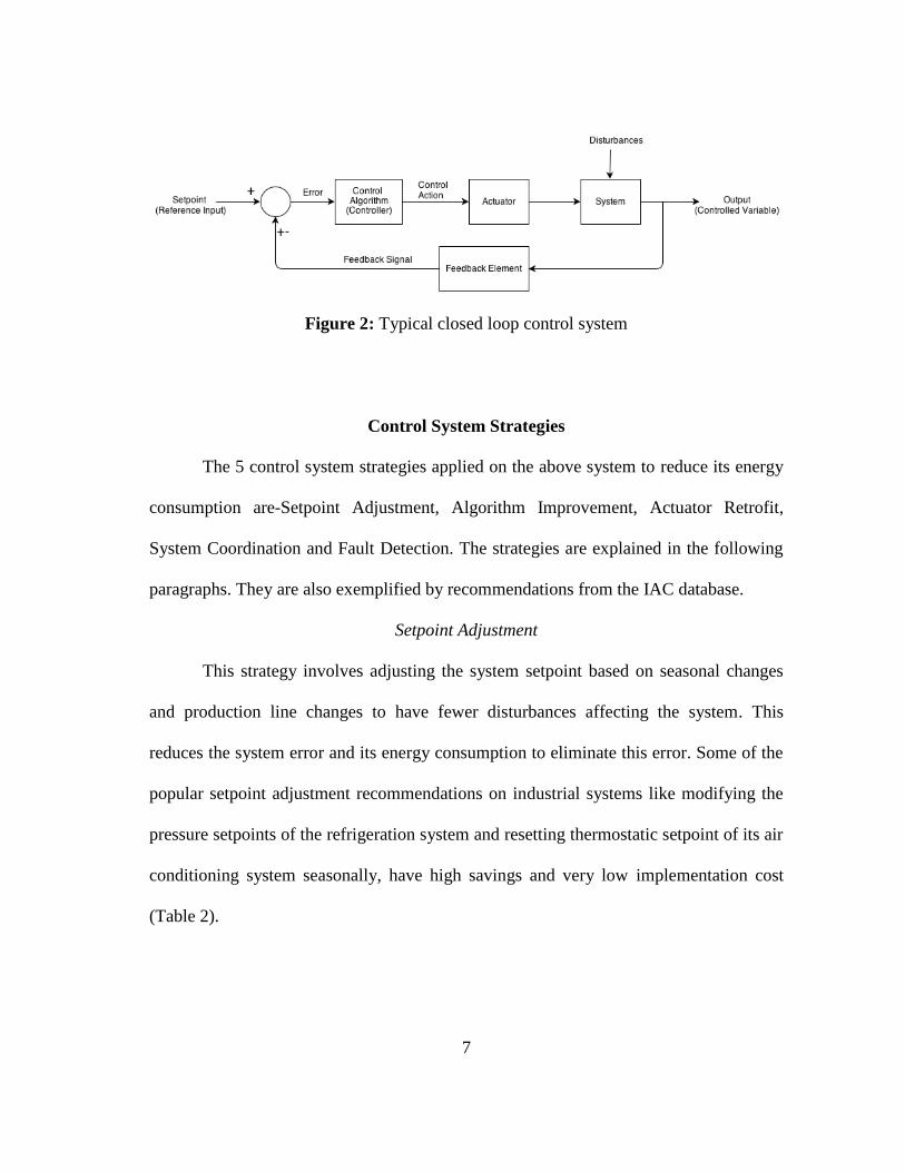
of a typical closed loop control system as shown in Figure 2.
The input to the control system is the desired value or the setpoint, which is
reached when the control algorithm that evaluates the error, or the difference between
the actual and desired output (carried by a sensor or the feedback element), decides an
appropriate control action to reduce it. This control action is then performed by the
actuator on the system till the system reaches its desired state. There may be
disturbances that adversely affect the output of the system which causes the control
system to continuously rework its actions so it can bring the system back to its desired
state.
7
Figure 2: Typical closed loop control system
Control System Strategies
The 5 control system strategies applied on the above system to reduce its energy
consumption are-Setpoint Adjustment, Algorithm Improvement, Actuator Retrofit,
System Coordination and Fault Detection. The strategies are explained in the following
paragraphs. They are also exemplified by recommendations from the IAC database.
Setpoint Adjustment
This strategy involves adjusting the system setpoint based on seasonal changes
and production line changes to have fewer disturbances affecting the system. This
reduces the system error and its energy consumption to eliminate this error. Some of the
popular setpoint adjustment recommendations on industrial systems like modifying the
pressure setpoints of the refrigeration system and resetting thermostatic setpoint of its air
conditioning system seasonally, have high savings and very low implementation cost
(Table 2).

8
Table 2: Common Setpoint Adjustment Recommendations
Description Times
Received
Average
Annual
Savings
Payback
(Years)
Implementation
(%)
Average
Energy Saved
(MMBTU/year)
Modify Pressure
Setpoints of the
Refrigeration
System
252 $19,630 1.5 35.17% 2,926
Reset
thermostatic
temperature
setpoints
seasonally
617 $10,157 0.3 62.79% 1,346
Reduce the
pressure setpoint
of compressed
air system
3,963 $3,792 0.5 49.29% 644
Reduce the
steam operating
pressure setpoint
148 $7,449 0.2 48.23% 1,638
Increase the
temperature
setpoint to the
highest possible
for chilling or
cold storage
37 $10,332 0.4 42.42% 1,311
Algorithm Improvement
The control algorithm directs the working of the actuator to deliver the desired
output. Therefore, by modifying the algorithm such that the least energy consumptive
action for the actuator is chosen, the equipment can be made more efficient. Therefore in
a facility that uses multiple pieces of equipment like compressors or boilers or chillers,
the algorithm can be modified so that the load is distributed to the most efficient set of
9
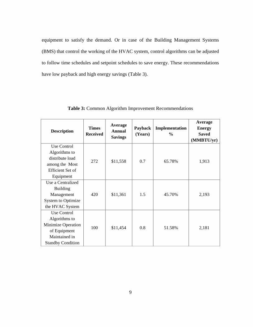
equipment to satisfy the demand. Or in case of the Building Management Systems
(BMS) that control the working of the HVAC system, control algorithms can be adjusted
to follow time schedules and setpoint schedules to save energy. These recommendations
have low payback and high energy savings (Table 3).
Table 3: Common Algorithm Improvement Recommendations
Description Times
Received
Average
Annual
Savings
Payback
(Years)
Implementation
%
Average
Energy
Saved
(MMBTU/yr)
Use Control
Algorithms to
distribute load
among the Most
Efficient Set of
Equipment
272 $11,558 0.7 65.78% 1,913
Use a Centralized
Building
Management
System to Optimize
the HVAC System
420 $11,361 1.5 45.70% 2,193
Use Control
Algorithms to
Minimize Operation
of Equipment
Maintained in
Standby Condition
100 $11,454 0.8 51.58% 2,181
10
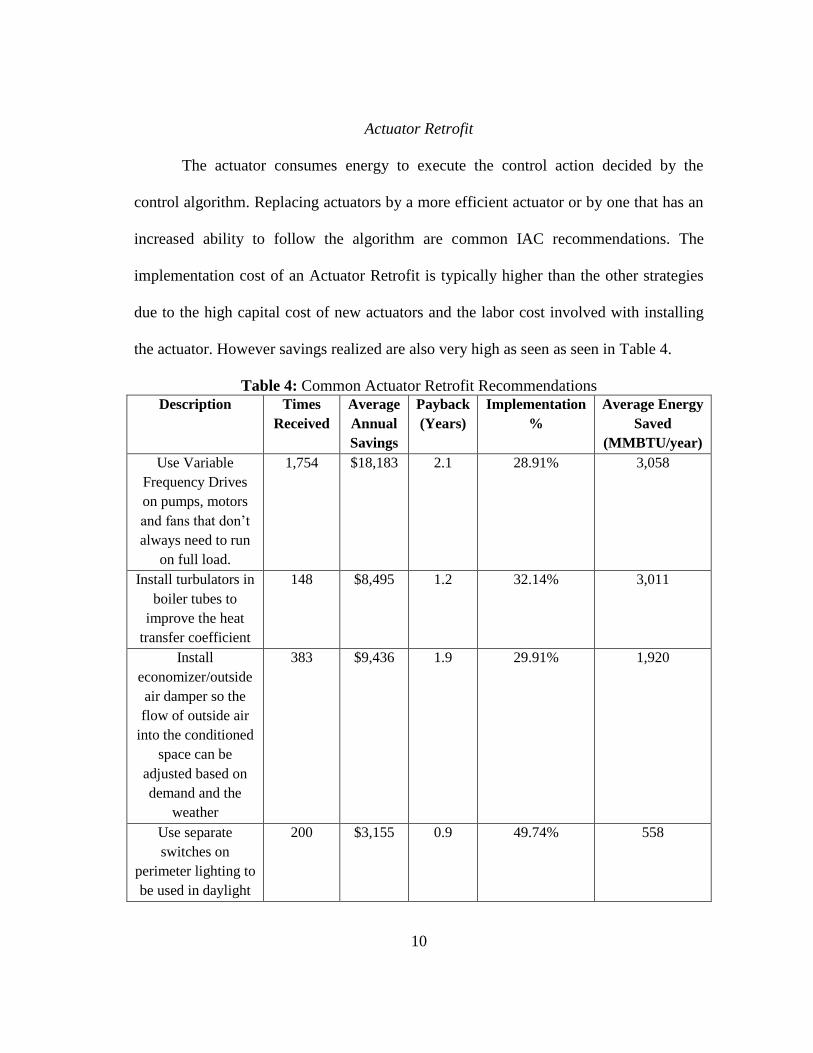
Actuator Retrofit
The actuator consumes energy to execute the control action decided by the
control algorithm. Replacing actuators by a more efficient actuator or by one that has an
increased ability to follow the algorithm are common IAC recommendations. The
implementation cost of an Actuator Retrofit is typically higher than the other strategies
due to the high capital cost of new actuators and the labor cost involved with installing
the actuator. However savings realized are also very high as seen as seen in Table 4.
Table 4: Common Actuator Retrofit Recommendations
Description Times
Received
Average
Annual
Savings
Payback
(Years)
Implementation
%
Average Energy
Saved
(MMBTU/year)
Use Variable
Frequency Drives
on pumps, motors
and fans that don’t
always need to run
on full load.
1,754 $18,183 2.1 28.91% 3,058
Install turbulators in
boiler tubes to
improve the heat
transfer coefficient
148 $8,495 1.2 32.14% 3,011
Install
economizer/outside
air damper so the
flow of outside air
into the conditioned
space can be
adjusted based on
demand and the
weather
383 $9,436 1.9 29.91% 1,920
Use separate
switches on
perimeter lighting to
be used in daylight
200 $3,155 0.9 49.74% 558

11
System Coordination
Using control systems, information can be exchanged by more than one type of
industrial system to coordinate their working. As the controller receives information
from multiple systems, it can oversee the operations of the overall process instead of a
single equipment. This control strategy, of synchronizing the working of interdependent
systems is System Coordination. A few good examples of this strategy are coordinating
the working of lighting and HVAC systems in a room, based on occupancy sensor
signals, and coordinating the working the turbine and boiler in a steam system. There are
not many examples of this strategy in the IAC database.
The above 4 strategies could ideally optimize the energy consumption of the
equipment. However in the real world there would be defects in the system over time
that need to be accounted for. If not corrected, these disturbances or faults will not only
increase the energy consumption of the system but also cause permanent damage to the
equipment. Therefore to help detect system faults and to avoid any production
downtime, one more control strategy is added to the list-
Fault Detection
This strategy involves using sensors to detect and diagnose any fault that
degrades the system performance. Typically, faults arise due to a defective sensor or
actuator. A faulty sensor that gives an incorrect reading of the variable it measures,
adversely affects any control algorithm that uses the same variable. A faulty actuator
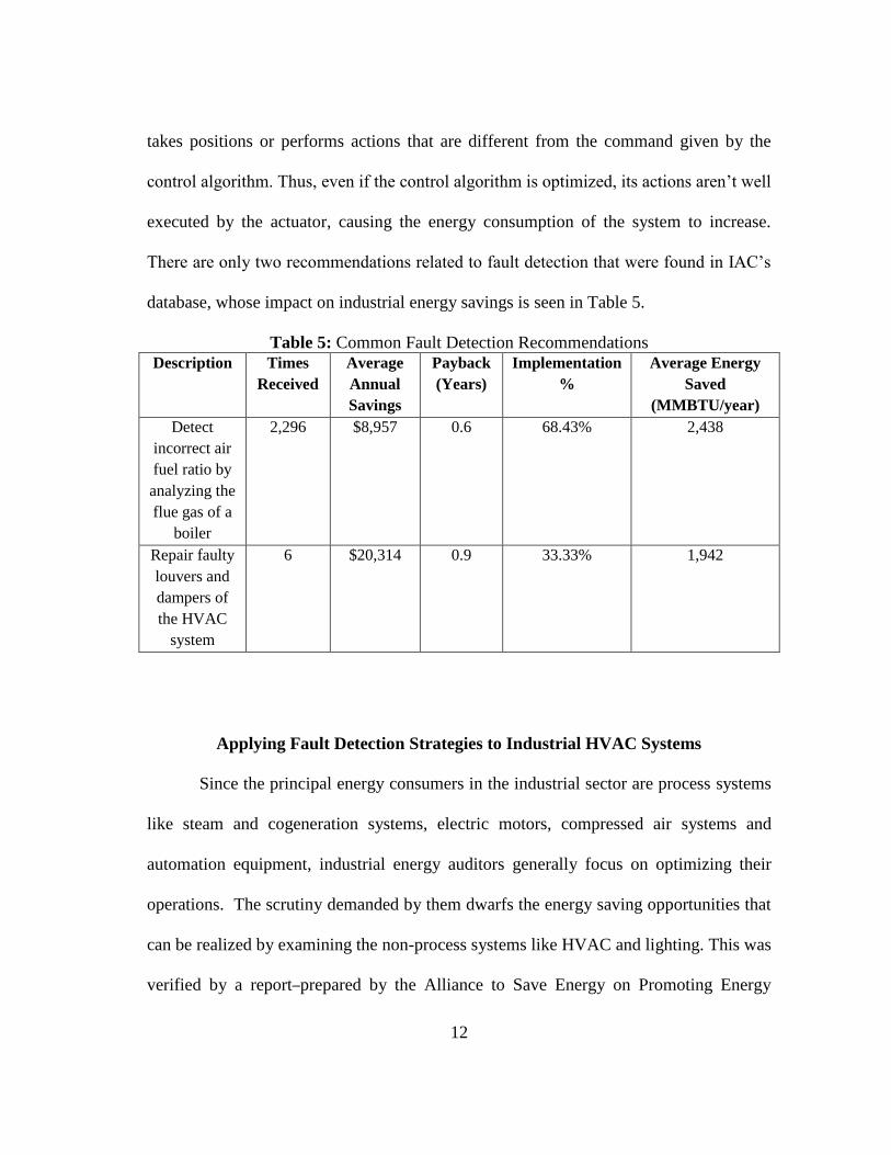
12
takes positions or performs actions that are different from the command given by the
control algorithm. Thus, even if the control algorithm is optimized, its actions aren’t well
executed by the actuator, causing the energy consumption of the system to increase.
There are only two recommendations related to fault detection that were found in IAC’s
database, whose impact on industrial energy savings is seen in Table 5.
Table 5: Common Fault Detection Recommendations
Description Times
Received
Average
Annual
Savings
Payback
(Years)
Implementation
%
Average Energy
Saved
(MMBTU/year)
Detect
incorrect air
fuel ratio by
analyzing the
flue gas of a
boiler
2,296 $8,957 0.6 68.43% 2,438
Repair faulty
louvers and
dampers of
the HVAC
system
6 $20,314 0.9 33.33% 1,942
Applying Fault Detection Strategies to Industrial HVAC Systems
Since the principal energy consumers in the industrial sector are process systems
like steam and cogeneration systems, electric motors, compressed air systems and
automation equipment, industrial energy auditors generally focus on optimizing their
operations. The scrutiny demanded by them dwarfs the energy saving opportunities that
can be realized by examining the non-process systems like HVAC and lighting. This was
verified by a report prepared by the Alliance to Save Energy on Promoting Energy

13
Efficient Buildings in the Industrial Sector. The report grouped the industrial
manufacturing subsectors into “building intensive” and “process intensive” categories.
The “building intensive” subsector included the Computers/Electronics, Heavy
Machinery, Transportation Equipment, Fabricated Metals, Foundries, Plastic/Rubber
Products, and Textile industries. And the remaining industries were grouped in the
“process intensive” subsector. According to the analysis, the building energy use ranged
anywhere from 4 to 41% of the total subsector energy use depending on how building
intensive the subsector was. And HVAC was responsible for about 70% of this building
energy use [5]. Since industrial buildings have higher HVAC loads and more operating
hours compared to residential and commercial buildings, the energy saved by optimizing
these systems could be significant. However according to IAC’s database of
recommendations, HVAC related recommendations make only 7% of all energy saving
recommendations. When these recommendations were organized based on the control
system strategy used, it was found about 45% of the HVAC system related
recommendations involved adjusting system setpoints, 20% involved improving the
algorithm and about 34% of them involved retrofitting the actuator. There are almost no
recommendations related to detecting faults in an HVAC system. This is in contrast with
commercial buildings where fault detection algorithms are extremely popular as they are
integrated in the facility’s computerized building management system. Small to medium
sized manufacturing facilities generally don’t have such advanced building management
systems to handle their air conditioning and lighting needs. This makes it tougher for
14
energy auditors to perform on-site measurements to detect a potentially faulty HVAC
system.
Therefore there exists the need for an automated fault detection and diagnosis
tool for air conditioning units found in these plants that can be used by energy auditors
to increase the scope of their assessment. The tool should be easy to install and should
not be too time consumptive. It should be able to detect faults by simple, low cost, non-
invasive measurements and predict the efficiency degradation due a fault. This would
help auditors perform cost saving and payback calculations when proposing a
recommendation. This thesis discusses the development of such a device to be used on
industrial energy audits by student technicians. The faults that the device can detect in a
unitary air conditioner are - an incorrect amount of refrigerant charge in the system
(undercharge or overcharge), a restriction in the refrigerant line of the air conditioning
system (liquid line restriction), and fouled heat exchanger coils (evaporator and
condenser fouling).

15
CHAPTER III
FAULTS IN UNITARY AIR CONDITIONING SYSTEMS
The HVAC equipment in small to medium sized manufacturing facilities are
generally unitary air conditioners (packaged and split units). Since these units are
smaller and more numerous, they are not as well maintained as larger HVAC systems.
They also lack advanced controls that would make scheduling their maintenance easier.
Periodic maintenance practices generally involve changing the evaporator filters, but
checking for leaks or restrictions in the refrigerant lines is a time consuming process for
HVAC technicians and is generally not done. Therefore these faults go undetected till a
loss in comfort is experienced. The wide spread prevalence of faulty air conditioners is
well documented by a number of researchers. In one of these studies carried out on light
packaged and split units in California, it was realized that about 70% of the investigated
systems had faults and about 40% of them had more than one fault. The estimated 10-
year cost savings for correcting these faults ranged from $800 to $1,700 per ton [6].
Before the types of faults and their effect on the performance of the system is
discussed, it is necessary to understand the principle behind air conditioning or the
Vapor Compression Cycle and the important terminology used in the thesis.
Background on Working of an Air Conditioner
Vapor Compression Cycle
The Vapor Compression Cycle shown in Figure 3 consists of 4 essential
components: a compressor, a condenser coil, an expansion valve and an evaporator coil.
The refrigerant absorbs the heat from the room by vaporizing on the low-pressure

16
evaporator side and rejects the heat to the ambient by condensing on the high-pressure
condenser side.
Figure 3: Components of the Vapor Compression Cycle
The energy exchange and phase change of the refrigerant through the system is better
explained with the pressure-enthalpy diagram shown in Figure 4.

17
Figure 4: Pressure Enthalpy diagram for the Vapor Compression Cycle
Evaporator (A to B-B’): A low temperature, vapor-liquid refrigerant mixture
enters the evaporator coil. It turns first into saturated vapor (Point B) and then
superheated vapor (point B’) by absorbing heat from the return air of the space.
Compressor (B’ to C): The superheated refrigerant then enters the compressor
at the suction side for isotropic compression. The compressor consumes work
(δW) to discharge the refrigerant as a high pressure, high temperature
superheated vapor.
Condenser (C to D’): The superheated vapor from the compressor enters the
condenser where the heat is rejected to the ambient (δQ2). This happens in three
stages: the vapor is first desuperheated (C to C’), then condensed (C’ to D), and
finally subcooled or cooled below its saturation temperature (D to D’). Thus the
refrigerant leaves the condenser as a single phase, subcooled liquid.
18
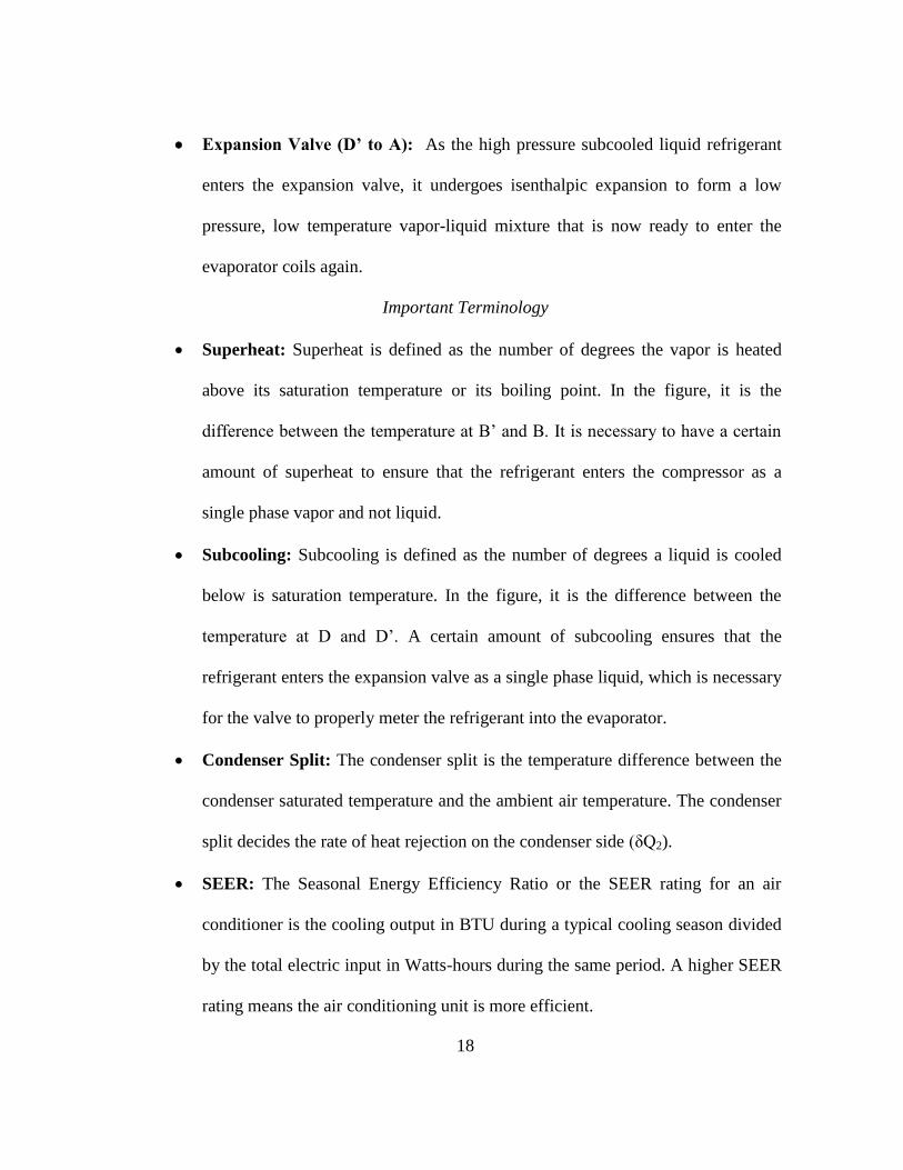
Expansion Valve (D’ to A): As the high pressure subcooled liquid refrigerant
enters the expansion valve, it undergoes isenthalpic expansion to form a low
pressure, low temperature vapor-liquid mixture that is now ready to enter the
evaporator coils again.
Important Terminology
Superheat: Superheat is defined as the number of degrees the vapor is heated
above its saturation temperature or its boiling point. In the figure, it is the
difference between the temperature at B’ and B. It is necessary to have a certain
amount of superheat to ensure that the refrigerant enters the compressor as a
single phase vapor and not liquid.
Subcooling: Subcooling is defined as the number of degrees a liquid is cooled
below is saturation temperature. In the figure, it is the difference between the
temperature at D and D’. A certain amount of subcooling ensures that the
refrigerant enters the expansion valve as a single phase liquid, which is necessary
for the valve to properly meter the refrigerant into the evaporator.
Condenser Split: The condenser split is the temperature difference between the
condenser saturated temperature and the ambient air temperature. The condenser
split decides the rate of heat rejection on the condenser side (δQ2).
SEER: The Seasonal Energy Efficiency Ratio or the SEER rating for an air
conditioner is the cooling output in BTU during a typical cooling season divided
by the total electric input in Watts-hours during the same period. A higher SEER
rating means the air conditioning unit is more efficient.

19
COP: The Coefficient of Performance or COP is a dimensionless representation
of the efficiency of an air conditioner. It is the ratio of the heat supplied or
removed from the room, to the work consumed by the air conditioner.
TXV: The Thermal Expansion Valve (TEV or TXV), is a metering device used
in the air conditioner for better control of the evaporator superheat. It controls the
amount of refrigerant flow to the evaporator based on the evaporator superheat.
A fixed orifice expansion device (FXO) on the other hand has a fixed opening
and cannot control the refrigerant flow.
EEV: Electronic Expansion Valves (EEVs) are a more sophisticated way of
controlling the refrigerant flow to the evaporator coil. The flow is controlled
using an electronic controller that sends signals to a stepper motor which controls
the opening and closing of the valve. Pressure and temperature sensors are wired
to the controller for better superheat and pressure control.
Faults in Unitary Air Conditioners
To identify what faults need to be included in the fault detection and diagnostic
device, a few fault distribution databases were considered. Stouppe and Lau recorded
the causes of over 15,000 air conditioning service calls over a period of 8 years (1980-
1987) [7]. About 76% of the failures were attributed to electrical components, 19% to
mechanical components and 5% to refrigeration circuit components. Most of the
electrical component failures were due to failures in motor windings, the mechanical
component failures were generally due to failed compressor valves, bearings, or
connecting rods. However what was not recorded in the survey, were the initial faults

20
that probably caused the eventual failure or loss in capacity of the system. The repair
costs associated with these service calls were also not recorded.
Breuker and Braun [8] created a database of 6,000 different fault cases and
analyzed the faults based on frequency of occurrence and repair cost of the fault. Based
on frequency of occurrence it was concluded that mechanical faults constituted 60% of
the total faults, and the remaining 40% of the faults were due to electrical and control
problems. Mechanical problems were mainly the refrigerant cycle problems associated
with the condenser, evaporator, compressor, and expansion device, or refrigerant charge
problems associated with the whole cycle. Electrical and controls problems involved
thermostat adjustments or replacements, wiring failure, damaged components, blown
fuses or bad connections. When the faults were analyzed based on the cost of repair, it
was concluded that the most expensive faults were related to compressor failures (24%)
due to its high cost component cost and labor cost to replace it. The combined refrigerant
cycle faults (condenser, evaporator, air handling unit and expansion valve) constituted
25% of the repair costs. The electrical and control related faults constituted 17% of the
total costs only because of their high frequency of occurrence.
Based on their findings it can be concluded that since the compressor is the most
expensive component to replace, frequent faults that may damage the compressor must
be included in the proposed device. A compressor generally gets damaged due to lack of
lubrication caused by presence of liquid in the compressor (liquid floodback). Liquid
refrigerant in the compressor shell acts as a solvent and washes the oil film from
adjoining surfaces like pistons, valves and rods in the compressor. This causes

21
overheating and scoring which damages the compressor components. It also dilutes the
lubricating oil thus compromising its ability to lubricate. The faults that could cause
liquid flooding could be evaporator fouling, condenser fouling, refrigerant overcharge or
a faulty expansion valve.
Therefore faults to be included in the fault detection device, were the ones that could
cause excessive loss of air conditioner performance and eventual component failure, the
faults that could lead to more expensive repair, and most importantly, what faults were
tougher to detect and diagnose in a typical maintenance visit. Based on the frequency of
occurrence and repair cost of faults, the following 5 faults were chosen to be detected by
the device:
Refrigerant Line Faults: Refrigerant Undercharge and Refrigerant Overcharge
and Liquid Line Restriction
Fouling Faults: Condenser and Evaporator Fouling
Refrigerant Line Faults
An air conditioning unit achieves its maximum cooling capacity and efficiency
when the amount of refrigerant it holds exactly matches the amount specified by the
manufacturer. If it is undercharged or overcharged, the performance and the life of the
system is affected. Since most air conditioners undergo final assembly at the customer
installation site, they are shipped from the factory with only enough charge for the
compressor and a fixed diameter and length of refrigeration line. For final installation,
charge has to be added or removed depending on the actual length of the tubing from the
indoor to the outdoor unit. Quite often, due to defects in the metering device, evacuation

22
techniques or other field installation problems, the system gets incorrectly charged and
fails to match the manufacturer’s specification [9]. As a result the system’s performance
will be affected due to the over- or undercharge.
Systems may also get undercharged over time due to leaks occurring at the pipe
fitting connections and through the walls of the copper refrigerant tubes over the years.
As refrigerant leaks out of the system into the open space, its high Global Warming
Potential (GWP) harms the environment. Older refrigerants like R-22 also have some
amount of Ozone Depleting Potential (ODP). Although these are phased out by the
Montreal Protocol and are found only in older systems, newer systems still use
refrigerants like R410A that have a global warming potential that is 2,088 times the
effect of CO2. Therefore checking the system for leaks as soon as an undercharge is
detected is very important.
To quantify the performance loss of the system due to refrigerant undercharge or
overcharge, a number of laboratory tests have been conducted over the years for systems
using different expansion devices and different refrigerants. Farzad & O’Neal (1993)
[10] conducted tests to find the loss in system performance due to incorrect R-22
refrigerant charge. Tests done on a fixed capillary system and a TXV system showed
that an undercharge of 15% reduced cooling capacity by 8 to 22% and EER by 4 to 16%
based on the outside air conditions. And an overcharge of 10% reduced the system’s
capacity by 1 to 9% and EER by 4 to 11%.
More recently, Kim and Braun [11] quantified the effect of different refrigerant
charge levels for systems using R-22 and R410A, in heating and cooling mode. The R-
23
22 system used a TXV and showed a 7% reduction in cooling capacity, and 9%
reduction in COP for a 30% undercharge. The R410a system showed a reduction of 70%
in cooling capacity and 65% reduction in efficiency for 60% undercharge. On the other
hand, overcharging by 30% increased the cooling capacity of both systems by 20% but
reduced their efficiency by 10%.
In spite of the performance degradation caused by incorrect refrigerant charge,
undercharged and overcharged systems have been widely prevalent. A report made for
the American Council for an Energy-Efficient Economy (ACEEE) in February 1999
listed the contributions of researchers that surveyed a number of residential air
conditioners and heat pumps, in existing and new homes. It was found that on average
refrigerant charge was either too high or too low in approximately three-quarters of the
central air conditioners and heat pumps tested. The report estimated an average energy
saving potential of 13% from all the studies of incorrect charge [12].
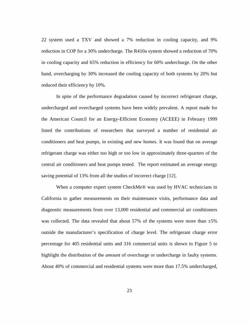
When a computer expert system CheckMe® was used by HVAC technicians in
California to gather measurements on their maintenance visits, performance data and
diagnostic measurements from over 13,000 residential and commercial air conditioners
was collected. The data revealed that about 57% of the systems were more than ±5%
outside the manufacturer’s specification of charge level. The refrigerant charge error
percentage for 405 residential units and 316 commercial units is shown in Figure 5 to
highlight the distribution of the amount of overcharge or undercharge in faulty systems.
About 40% of commercial and residential systems were more than 17.5% undercharged,

24
and at least 25% of commercial systems and 32% of residential systems were more than
7.5% overcharged [13].
Figure 5: Refrigerant Charge Error Percentage in surveyed Residential and Commercial
Systems [13]
The best way to identify an incorrectly charged system is to look for abnormal
pressures and temperatures. The only other way to detect these faults would involve
removing all the charge from the system and weighing it, which is an expensive and
time-consuming process. The impact of the faults on system performance, and how they
affect the temperatures and pressures in the system was explained in a series of articles
by Mr. John Tomczyk for ACHR News[14, 15]. His explanations are summarized in the
following sections to help identify the symptoms of the faults.
25
Refrigerant Undercharge
An undercharged system has lower cooling capacity, and it may cause overheating
and eventual failure of some parts of the system. Its effect on individual components is
explained below.
Evaporator: In an undercharged system, all the components are starved of
refrigerant. The starved compressor trying to draw refrigerant into its cylinders
causes a low pressure on the evaporator side of the system. Evaporator pressure
being low implies that its saturation temperature is low. This means for the same
amount of heat absorbed at the evaporator and the reduced amount of refrigerant,
the refrigerant evaporator exit temperature will be higher, or the superheat will be
high.
Compressor: Since the compressor sees more superheated, lower density vapors,
its amperage draw is lower. As it compresses the vapor, the superheat increases
even more, increasing the discharge temperature at the compressor outlet.
Condenser: The starved condenser does not see as much heat to reject to the
ambient. Therefore, it has a lower temperature and pressure and a low condenser
split. Its 100% saturation point is very low since there is lesser refrigerant vapor
to condense into a liquid, thus reducing the condenser subcooling.
Therefore the symptoms of an undercharged system are:
Low evaporator pressure
High superheat
Low compressor amperage draw
26
High compressor discharge temperature
Low condenser split
Low subcooling
Refrigerant Overcharge
Refrigerant overcharge may not reduce the cooling capacity, but certainly reduces
the efficiency of the system and may potentially damage the compressor. The effect of
refrigerant overcharge on the individual components of the system is explained below.
Condenser: When the system gets overcharged, the excess refrigerant is backed
up in the condenser as a subcooled liquid. Therefore a greater percentage of
condenser tubing holds liquid, leaving lesser tubing for the vapor to undergo
condensation. To reject the same amount of heat with the reduced area entails
increasing the “condenser split” or the temperature difference between condenser
saturated temperature and the ambient temperature. Thus, the condenser saturated
temperature increases, and the corresponding condenser saturated pressure also
increases. The excess subcooled refrigerant also increases the condenser
subcooling.
Evaporator: If the system uses a thermal expansion valve, the evaporator pressure
will be normal to slightly high depending on the amount of overcharge, and the
TXV will try to maintain normal superheat even at excessive overcharge.
However, in case of a fixed orifice expansion device the superheat will be lower
and the evaporator pressure will be higher.

27
Compressor: Due to the higher condenser pressure, the compressor will have to
do more work to compress the refrigerant to this pressure. Thus the amperage
draw of the compressor will be more, as will its compression ratio and discharge
temperature. At higher levels of the fault, the excess refrigerant may not vaporize
completely in the evaporator thus entering the compressor as a liquid. Liquid
refrigerant in the compressor can cause slugging or flooding of the compressor,
and compressing the liquid will cause permanent damage to the valves of the
compressor.
In summary, the following are the symptoms of an overcharged air conditioner: .
High subcooling
High condenser split
High condenser pressure
Normal to high evaporator pressures
Low superheat in case of fixed orifice expansion device
High compressor amperage draw
High discharge temperatures
The other refrigerant line fault that may develop over time due to poor maintenance
of the air conditioner is liquid line restriction. The liquid line is the refrigerant line
between the condenser outlet and the expansion device inlet. The refrigerant flow in this
line may get restricted due to a clogged filter/drier or a TEV strainer, or a kinked up
liquid line. This causes low pressures downstream of the restriction, resulting in loss of
cooling capacity due to the reduced refrigerant flow in the evaporator, or in some cases

28
severe damage to the compressor. Rossi and Braun (1997) showed that a 20% increase in
pressure difference across the liquid line due to a restriction could cause a 17% loss in
capacity and 8% loss in COP [8].
A crude way of detecting liquid line restriction is by looking for a cold spot
somewhere on the liquid line, downstream of the restriction, since the pressure drop due
to the restriction causes some amount of liquid flashing. By running the hand over the
liquid line, near the filter drier a cold spot could be found. However, the human hand is
not capable of sensing temperature differences less than 10°F, thus the restriction could
go undetected. If the system has a sight glass just after the restriction and before the
expansion valve, bubbling in the sight glass could also be an indication of liquid line
restriction, but this may not be always true. Bubbles in sight glasses are seen due to
various other reasons like rapid increases in loads or undercharge. Therefore the best
way to confirm the fault is to look for the symptoms of the fault whose presence is
explained as follows [16].
Liquid Line Restriction
The symptoms of liquid line restriction and its effect on the components of the air
conditioning system are explained as follows:
Expansion Valve: The restriction in the liquid line introduces an additional
pressure drop. This pressure drop causes some of the liquid refrigerant to
vaporize before it reaches the expansion valve, which affects the functioning of
the expansion valve as it now sees a two-phase mixture instead of a pure liquid.

29
Evaporator: Since components downstream of the restriction are starved of
refrigerant, more refrigerant is drawn from the evaporator by the compressor.
Now the evaporator is starved of refrigerant and it will have a lower pressure.
This implies the evaporator saturated temperature is also lower, which means for
the same amount of heat load the evaporator superheat will be higher. With a
restriction in the liquid line that affects the inlet to the expansion valve, the TEV
cannot be expected to control superheat as well as it would.
Compressor: The compressor may get severely overheated due to the lack of
refrigerant that would otherwise keep it cool. This means that the discharge
temperatures of the compressor will be high. Its amperage draw will be low since
there is lesser refrigerant and lower density refrigerant enter the compressor.
However, it may short cycle due to the low pressure on its suction side, and once
some refrigerant enters it to increase its pressure, it would go on again. This will
keep occurring till it gets overheated. Short cycling will cause damage to the
compressor motor and capacitors.
Condenser: The restriction causes lesser refrigerant to flow through the system.
Lesser heat is introduced in the condenser, since lesser refrigerant enters the
condenser from the evaporator and compressor. Since lesser heat has to be
rejected, the condenser split need not be high. Thus the condenser saturated
temperature (and therefore condenser pressure) is lower. The refrigerant backs up
into the condenser due to the restriction and gets more subcooled.
Therefore a summary of the symptoms is:

30
Low evaporator pressure
High superheat
High compressor discharge temperature
Compressor short cycling
High condenser subcooling
Fouling Faults
For an air conditioner to adequately heat or cool a space, its heat exchangers need
to be able to absorb and reject heat at a sufficient rate. This rate is a function of the
temperature difference between the refrigerant in the tubes and the air crossing the tubes,
the surface area of the tubes exposed to the air and the heat coefficient of the tubes.
Since the temperature difference depends on the operating conditions, to ensure that the
system can cool or heat the space up to its capacity, it is important to keep the coils clean
thus ensuring sufficient area for heat exchange.
As the condenser coil is placed outdoors, its coils get covered with leaves, dust,
wool, pollen and dust, thus reducing the effective air flow over the coils. When the
condenser fouling is severe, the system can’t reject heat at a fast enough rate causing all
its parts get overheated resulting in component damage reduced system efficiency. In
case of the evaporator, the evaporator filter may clog up with dirt, thus reducing the air
flow to the evaporator coil. If the evaporator fouling is severe enough, the refrigerant
fails to vaporize and enters the compressor as liquid, permanently damaging its parts.
To quantify the loss in system efficiency due to evaporator fouling, Breuker and Braun
[8] conducted tests on a three ton packaged air conditioner that used a fixed orifice

31
expansion device. They simulated the condenser fouling fault by covering the condenser
with strips of paper. The evaporator filter fouling fault was simulated by changing the
speed of the air flow across the evaporator by using a variable speed fan. The resulting
decrease in cooling capacity varied from 3 to 11% for condenser fouling of 14 to 56%.
The corresponding decrease in COP was 4 to 18%. The decrease in cooling capacity for
evaporator fouling from 12 to 36% varied from 6 to 19% and the COP decreased by 6 to
17%.
Some industrial facilities have ‘clean rooms’ that use a high efficiency filter,
others have excess dust and dirt in the return air due to manufacturing operations carried
on in the air conditioned space which can easily clog up even a low efficiency filter. Li
and Braun [17] tested impact of evaporator fouling on the performance of the air
conditioner and heat pump for different levels of filtration. For one year’s dust loading
(600 grams of dust), the 35 ton, 5 ton and 3 ton units had EER degradations ranging
from 2% to 10%. Lower degradation for lesser efficient filter and bigger sized units.
In the report prepared for ACEEE that summarized the work of researchers that surveyed
a number of residential air conditioners and heat pumps, it was found that nearly 70% of
indoor air coils had inadequate air flow (where normal air flow was considered to be 400
cfm per ton of cooling capacity). The average airflow of the faulty systems was nearly
20% below the manufacturer’s recommended airflow. The report estimated an average
energy saving potential of 8% for such units [12]. In a different study that surveyed more
than 13,000 systems in California, it was found that at least 21% of the systems had low
evaporator air flow problems [13].

32
Although fouling faults are visible, their detection is automated by the proposed
device by making use of the abnormal pressures and temperatures caused by these faults.
These symptoms are summarized in the following sections.
Evaporator Fouling
The effects of a fouled evaporator coil or clogged evaporator filter on each
component of the system are explained as follows.
Evaporator: Since a fouled evaporator filter does not allow as much warm return
air to enter, the refrigerant in the evaporator may not get superheated enough, or
in some severe cases of fouling, it may not even get vaporized. Thus the
temperature and pressure in evaporator is low. Sometimes, frost forms on the
exterior of the evaporator coil since the low temperature refrigerant inside has
not picked up enough heat. This frost further impedes the heat exchange at the
evaporator coil.
So if the evaporator coil is fouled, there is lesser surface for heat exchange for
the warm return air, resulting in insufficient cooling of the air. Therefore the
temperature difference of air across coil decreases. But in case the evaporator
filter is fouled, there is lesser air coming in contact with the coil, resulting in
overcooling of the air. Therefore for evaporator filter fouling the temperature
difference of the air across coil increases.
Compressor: If the refrigerant in the evaporator is not completely vaporized, it
may enter the compressor as a liquid. This will cause flooding of the crankcase in
the compressor and dilution of the compressor oil. Since the refrigerant entering

33
the compressor is less superheated and has a greater density, it increases the
amperage draw of the compressor.
Condenser: Since the fouled evaporator does not absorb much heat from the
space, the condenser has lesser heat to reject to the ambient surrounding. Thus it
doesn’t need to have a very high condenser split. This implies the condenser
saturated pressure and temperature does not need to be too high either.
Thus the symptoms to look for when detecting a fouled evaporator are-
Low evaporator superheat
Temperature difference of air across evaporator high in case of fouled evaporator
filter and low in case of fouled evaporator coil.
Frost on the evaporator coils, or refrigerant lines entering the compressor
Lower compressor discharge temperature
Low condenser split
Low condenser pressure
Condenser Fouling
The effects of condenser fouling on the individual components of the system are
explained as follows:
Condenser: Heat from evaporator, compressor motor, suction line and from the
compression of the refrigerant is all rejected in the condenser. If the condenser
coil is fouled, the condenser cannot reject this heat fast enough. This means to
increase the rate of heat rejection, the condenser split (or the difference between
the condenser saturated temperature and outside air temperature) is increased.

34
Due to the pressure-temperature relationship, a higher condenser saturated
temperature would imply a higher condenser pressure.
Therefore, since the area exposed to the ambient air is reduced, to dissipate the
same amount of heat, the temperature difference of the air across the coil
increases.
Evaporator: Since all the heat absorbed by the refrigerant in the evaporator is not
rejected by the condenser at a fast enough rates due to a fouled coil, the
evaporator may not be able to cool the space up to its potential. In cases of severe
condenser fouling, the high condenser pressure may cause the evaporator side
pressure to slightly increase as well.
Compressor: Since the condenser pressure is higher, the compressor has to work
harder or draw more current to compress the refrigerant to the higher pressure.
The high heat of compression from the higher compression ratio will increase the
discharge temperature of the compressor.
Therefore the symptoms of a fouled condenser are:
High condenser split
High condenser pressure
High evaporator pressure
High compression discharge temperature
High temperature difference of air across condenser coil
35
Looking for abnormal pressures and temperatures in an air conditioning system is the
best way to correctly detect and diagnose the faults affecting it, as it requires non-
invasive, low cost measurements. However, to know if the measured temperature and
pressure is too high or too low, we first need to know what temperatures and pressures to
expect. With the wide variety of air conditioning systems in terms of size, type, working
in different operating conditions, this requires the expertise and knowledge of an
experienced technician. Moreover, incase an overcharge or undercharge is detected,
there is no way for the technician to predict the amount of incorrect charge and the
related efficiency loss. The proposed device tries to overcome these challenges. It uses
the listed symptoms along with typical thresholds to make fault detection and diagnosis
simpler for student energy auditors.
36
CHAPTER IV
LITERATURE REVIEW
Introduction to Fault Detection in HVAC Systems
In early 1970s fault detection and diagnosis (FDD) was explored for use in life-
critical systems and processes in the fields of nuclear power, aerospace, process controls,
automotives, manufacturing, and national defense. FDD in these fields were developed
to improve safety and reliability of the equipment and to prevent loss of life. Research in
FDD in the air conditioning and refrigeration field was only explored after the
decreasing cost of microprocessors and hardware over the years made it economically
viable. Numerous surveys of air conditioners and refrigerators by investigators aided by
technicians helped realize the wide spread prevalence and effects of faults in HVAC
systems.
Researchers mostly referred to Isermann’s (1978) generic method of fault
detection and diagnosis to develop their FDD method for HVAC&R [18]. FDD is made
of three key steps. The first step is Fault Detection which involves checking if a
particular measureable or unmeasurable signal was within a certain tolerance of the
normal value. This is followed by Fault Diagnosis which identifies the location and
cause of the fault. FDD for HVAC in particular includes a third step which is Fault
Evaluation which involves analyzing the short term and long term effects of the faults to
check if the benefit of servicing justifies its expense. This is different from FDD in
critical systems which has zero tolerance for faults and requires no decision making.

37
FDD in HVACR was first tried in the late 1980s for fault detection in household
refrigerators by Mc Kellar in 1987 [19] and Stallard in 1989 [20]. The faults considered
were compressor valve leakage, heat exchanger fan failures, frost on the evaporator,
partially blocked capillary tube, and refrigerant charging failures. McKellar found that
each of these faults had unique effects on three measures: suction pressure, discharge
pressure, and discharge-to-suction pressure ratio and concluded that these measures were
sufficient for developing a FDD system. Based upon the work of McKellar, Stallard
(1989) developed an expert system for automated FDD applied to refrigerators.
Directional change of measured quantities like condensing and evaporating temperatures
and discharge and suction pressures, with respect to expected values were used to
diagnose faults.
Since this first attempt, HVAC FDD has seen a growth in interest from
researchers. This is seen by the increasing number of papers related to the topic since
1996 [21]. Although half of these papers focused on FDD for air handling units and
variable air volume terminal boxes, FDD in vapor compression systems like chillers and
packaged air conditioners still saw lesser but significant contributions.
FDD was applied to chillers by Grimmelius et al. in 1995[22] . A cause and
effect analysis for different faults was developed to arrive at a failure symptom pattern
for each fault. By using a reference regression model, and over 20 different
measurements of temperature, pressure, power consumption and oil level, residuals were
generated. A residual pattern particular to a fault mode was developed and faults were
diagnosed by scoring how well the fit was into a residual pattern. Stylianou and

38
Nikanpour (1996) [23] used a similar pattern matching approach, but instead used a
thermodynamic model in their FDD system. In fact, their FDD system was divided into
three parts- one when the chiller is off, one during start up and one during its steady state
operation. They required 17 different temperature, pressure and flow measurements to
refrigerant leak, refrigerant line flow restriction, condenser waterside flow resistance,
and evaporator waterside flow resistance.
Jia and Reddy (2003) [24] used a characteristic parameter approach, to detect and
diagnose faults in chillers. The performance of every component of the chiller (motors,
heat exchangers etc.) is quantified by one or two parameters. Since each parameter is
indicative of the health of a particular component, fault detection and diagnosis is easier.
This method however is suitable only for larger HVAC systems that generally have
numerous sensors.
Fault Detection Methods in Unitary Air Conditioners
Although majority of FDD algorithms were made for chiller and air handling
units, interest in FDD on residential, low tonnage air conditioners, that is, split and
packaged direct exchange systems grew due to two reasons: because these systems are
used widely and because are not very well maintained by their owners.
FDD in unitary air conditioners was first attempted by Yoshimua and Noboru in
1989 who used a combination of six temperature and two pressure measurements to
perform FDD for packaged water cooled and air cooled air conditioners of a
telecommunications building [25]. They developed an algorithm to detect condenser and
evaporator coil fouling, and detect an abnormal evaporator and chilled water pump

39
operation. They used superheat, subcooling, ratio of rated and actual condenser pressure
and evaporator pressure and the temperature difference of air across the evaporator and
air (or water) across condenser, as their six diagnosis parameters. These diagnosis
parameters were compared to fixed thresholds as per a diagnostic flow diagram to detect
the faults. Expected values of pressure and temperatures were obtained from the
manufacturer and they were compared to the actual values. Actual test results, or any
information about the threshold values and the sensitivity of the method is not provided.
Rossi and Braun (1997), developed the statistical rule based model using 9
temperature measurements and one humidity measurement to successfully detect and
diagnose five faults: leaky compressor valve, liquid line restriction, evaporator filter
fouling, condenser fouling and refrigerant undercharge [26]. A steady state model was
used to relate operating conditions of the system (ambient temperature, indoor
temperature and humidity) to the expected output states occurring at no-fault conditions.
These expected output states were temperature measurements at different points in the
vapor compression system, and they were compared to actual temperature measurements
to generate residuals. Fault detection was achieved by evaluating the statistically
evaluating these residuals. The overlap of the residual probability distribution for a
normal and faulty operation was the classification error, which reduced as the level of
fault increased. For fault diagnosis, directional changes of the residuals were related to a
specific fault based on a set of rules. Diagnosis was done when the probability of the
most likely fault is greater than the probability of the second most likely fault by a
certain threshold. The method was tested and evaluated on a 3 ton rooftop unit that used

40
a fixed orifice expansion device. It could detect and diagnose a 2% reduction in
refrigerant charge, 5% compressor valve leak, 20% condenser fouling, and 40%
evaporator fouling. In the laboratory tests, liquid line restriction could only be detected
at a level greater than 80%. The method didn’t require any equipment specific
experimentation since the diagnostic rules were generic. However the method also
requires the development of a model for the system which is time consuming and
expensive as the model needs to be trained over a wide range of conditions. It also
introduces modeling errors to the method.
The FDD sensitivity is greatly improved by using model-based pre-processing
and statistically based thresholds, but these system specific models require extensive
experimentation for each fault. Since the faults need to be detected in smaller HVAC
systems that are inexpensive themselves, the software and hardware related to the FDD
for the systems need to be less expensive too for it to be economically viable.
Therefore to eliminate the requirement of an expensive measurements and a
model that requires extensive testing, Chen and Braun (2000) came up with two
methods- the “Sensitivity Ratio Method” and the “Simple Rule Based Method” to detect
faults in unitary air conditioners [27]. The faults detected were evaporator and condenser
fouling, refrigerant overcharge and undercharge, liquid line restriction, non-condensable
gas and compressor valve leakage. Unlike Rossi’s tests in 1995, the tests were done on a
5 ton rooftop unit that used a thermal expansion valve instead of a fixed orifice valve. In
his first method, the “Sensitivity Ratio Method” a unique pair of sensitive and
insensitive residuals were used to calculate sensitivity ratios for each fault. If a fault
41
occurred, the value of the ratio would go below a preset threshold and fault would be
detected. A noise filter was used so if the residual was less than 2°F, it was reset to
0.1°F. In this way if the system was faultless the sensitivity ratio would be 1, and if the
ratio went below 1 a fault was detected. These checks against thresholds were done in a
methodical way using a diagnostic flow chart developed by the authors. 11% LLR, 20 to
30% condenser fouling, 7 to14% evaporator fouling, 5 to 10 % undercharge and 10%
overcharge and 0.09% non-condensable gas were the minimum fault levels that were
sensitive to this method.
The second method- “Simple Rule based method” performed just as well as the
first without the use of a model to generate residuals. It required only six temperature
measurements and no humidity measurements. It used performance indices computed
from raw measurements that are independent of operating conditions but are sensitive to
the fault. The performance indices were liquid line subcooling, condenser split,
evaporator split, temperature difference across liquid line, and evaporator split. There is
a unique pattern of change of these performance indices for the different faults, and the
thresholds to detect a fault using these performance indices were experimentally
determined at different conditions. This method works well for low cost FDD
applications. However, like the other fault detection methods developed so far, this
method couldn’t detect multiple faults.
In 2007, Li and Braun developed a decoupling methodology to detect multiple
simultaneous faults in a system. The authors use ‘decoupling features’ that are uniquely
dependent on individual fault, as the key to handling multiple simultaneous faults. The

42
decoupling features for the faults were identified as evaporator and condenser volumetric
air flow rate for evaporator and condenser fouling, compressor discharge temperature for
compressor valve leakage, a refrigerant charge indicator that used subcooling and
superheat to detect incorrect refrigerant charge and pressure difference across the
expansion valve was used to detect liquid line restriction. For fault detection, a fault
indicator was calculated as the ratio of the current value of the decoupling feature to its
value for a 20% cooling capacity loss. For all the different combinations, 41 different
tests were done on a 5 ton rooftop unit using at TXV. Multiple fault diagnosis was done
using a modified error indicator where the decoupling feature for an individual fault and
case and a multiple simultaneous fault case were related. Based on the results of the 41
different tests, the authors concluded that only two false alarms occurred for the 41
different fault combinations and a sensitivity loss for LLR fault occurred.
The challenge with such a method was that measuring some of the decoupling
features like liquid line pressure, air flow rate and refrigerant mass flow rate would
require expensive sensors. Therefore Li and Braun also developed ‘virtual sensors’ that
would use thermodynamic relations and map models of compressors and expansion
valves to calculate the decoupling features from low cost temperature measurements
[28]. Compressor power consumption and mass flow rate of refrigerant was predicted
using the compressor map model which is a 10 coefficient polynomial available from
manufacturers. The prediction accuracy was within 5% of actual value. Volumetric air
flow rate across condenser and evaporator and expected compressor discharge
temperature were calculated using thermodynamic relationships.

43
A different approach to fault detection worth citing was tried using electrical
signal measurements instead of temperature and pressure measurements [29]. This
approach of Non-Intrusive Load Monitoring used the starting transient signals and
reduced them to ‘signatures’. Changes in the signatures helped detecting faults in the
system. The advantage of this approach was that it reduced the number of measurements
needed; but it also made device expensive and system specific.
Therefore, the final device could not use the Statistical Rule Based method,
Sensitivity Ratio method or the Non-Intrusive Load Monitoring method in its algorithm,
as these methods require an online model. Since the device is meant to be portable and
needs to be able to work with different types and sizes of equipment, developing a model
is expensive and time consuming. The decoupling method also cannot be used in the
proposed device, as it requires information of compressor map models that is not easily
available to student technicians. The challenge is to achieve fault detection and diagnosis
with minimal, easy to obtain information. Thus the proposed device uses an algorithm
that is based on the Simple Rule Based method. However, it goes a step ahead as it tries
to achieve multiple fault detection.
Existing Commercial FDD Devices in HVAC
Fault detection in HVAC has seen growing popularity over the past few years. In
mid 1990s an ASHRAE Technical Committee on Smart Buildings became active in
FDD research. The 2013 California Title 24 energy code (California Energy
Commission [CEC] 2012) now requires FDD on all newly installed unitary equipment.
As a result, now there are several equipment manufacturers who include FDD

44
capabilities in some of their unitary equipment product lines. However, FDD in HVAC
is still in its infancy when compared to other fields like automobiles, where FDD has
been incorporated for more than a decade. Much of the research and development in
FDD for HVAC&R is still performed in universities and national laboratories and there
are only a few commercialized tools available on field which use these techniques [30].
Some indicate operational faults in the system, the others continuously monitor the
performance of the system to indicate the presence of a possible fault. Some of these
devices are:
1. Virtjoule: Virtjoule uses non-invasive electricity and/or vibration sensors that
are attached to the outside of the air conditioning unit [31]. The device monitors
compressor and outdoor fan operation and analyzes this data to catch air
conditioner failures before they occur. The sensor data can be accessed real-time
via a web application where alerts for under-cycling or over-cycling, non-
operation can be created. This would also help the user know if the air
conditioner is left running after operating hours.
2. Smart Monitoring and Diagnostic System (SMDS): The SMDS was developed
to detect a change in performance in the refrigerant side of the packaged air
conditioning systems. Therefore it can be used to quantify the impact on the
performance and the cost savings resulting from servicing. It can help the
building owner decide when to schedule servicing based on increased energy cost
due to performance degradations and servicing costs [32]. It detects operational

45
faults in the system like – supply fans always being on, compressor always being
on, RTU always off and supply fan cycling.
3. FDSI- Synergy: Synergy is a software application that uses data from the
building management software, and uses mathematical models and fault
detection algorithms to detect the faults existing in the air conditioning unit. It
collects set points, run times, interior and exterior temperatures daily, and uses
the facilities’ utility data (peak demand and electricity cost), to estimate possible
cost saving opportunities. It organizes these cost saving opportunities in different
categories- based on difficulty, urgency, payback period and equipment type.
4. Sensus MI: Sensus MI is an automated fault detection system to give an early
indication if a machine is working properly or installed properly to the service
company [33]. The device continuously learns about the equipment, as it can
diagnose a few faults like incorrect refrigerant charge or a dirty evaporator or
condenser coil. As the service company technician can view the condition of the
system on a dashboard in his office, it helps the company schedule their
maintenance visits better, before there is significant discomfort felt by the users
of the HVAC system, or before the system completely breaks down.
5. ClimaCheck: ClimaCheck technology can detect faults in air conditioning
systems in two ways- a fixed installation as well as a field inspection unit [34].
The field inspection units uses a current measurement, 7 temperature
measurements and two pressure measurements to define actual performance and
compare it to the ideal system performance. It is used to estimate the cost and
46
benefits of operational improvements and optimization. It can be integrated with
the building management system for chillers and heat pumps, as a portable
performance analyzer.
Almost all of the above devices (SMDS, Synergy, Virtjoule, Sensus MI) require
permanent installation on the air conditioning unit. They are made either for the building
owner or from the point of view of a service technician. They need to collect data from
the system over a long period and are not portable or made for energy auditing purposes.
Some of them can only predict operational faults (cycling, incorrect fan operation etc.)
but not system faults like refrigerant over- and undercharge (Virtjoule, SMDS). The
device that comes close to meeting these challenges (ClimaCheck) is too expensive and
relies on a large database for its working. It is unclear whether the portable ClimaCheck
device can diagnose all faults, or only sets off an alarm when a reduction in the
performance of the system is detected.
The following chapters explains the development of the proposed device that can
meet these challenges of portability, low cost, and cost saving prediction.

47
CHAPTER V
DEVELOPMENT OF THE PROPOSED ALGORITHM
Developing a robust fault detection and diagnostic algorithm for air conditioners
had many challenges.
The rules and thresholds chosen had to work for a wide range of
operating conditions such as diverse climates and weather conditions.
The sensitivity of the system was a tradeoff for avoiding false alarms or
overestimation of energy and cost savings.
The algorithm also had to be kept as generic as possible so it could work
for a wide variety of air conditioner types and sizes found in the
industries.
The proposed algorithm tries to meet these challenges while meeting the
requirements of the device- easy to use, quick, portable and low cost, with the ability to
evaluate a detected fault. The majority of the work for the development of the device
was done using data generated at the Thermo-Fluids Controls Laboratory (TFCL) by
introducing known faults to a system to test the algorithm. This chapter will discuss the
development of the proposed fault detection and diagnosis algorithm and its
components.
Background to the Proposed FDD Method
While developing the Statistical Rule Based method, Rossi and Braun [26]
divided their FDD algorithm into a preprocessor and a classifier. The preprocessor
would calculate ‘features’ from actual measurements which were used by the classifier

48
for fault detection and diagnosis. Fault detection classifier has a binary output – fault or
no fault, and the fault diagnostic classifier has to choose from a list of faults.
The preprocessor could generate features of three types: simple transformations,
characteristic quantities or model residuals. Simple transformations involve generating
time derivatives or trends to detect faults. Characteristic quantities involve generating
features that are directly calculated from measurements, and model based preprocessors
use mathematical models to predict the performance, which is compared to the actual
performance of the system to generate residuals as features that would be used by the
classifier. Since the proposed fault detection device is intended to be quick, and would
collect data for less than an hour a time derivative approach isn’t used. Developing a
mathematical model would make the device very specific to only a certain type and size
of air conditioner, which is also not desired. Therefore, the proposed fault detection
algorithm uses a preprocessor that generates characteristic quantities from actual
measurements. The characteristic quantities or features are used by the classifier for fault
detection and diagnosis.
The method chosen for the working of the preprocessor and classifier is loosely
based on the Simple Rule Based method put forward by Chen and Braun [27]. In that, it
uses 7 performance indices or features that are insensitive to operating conditions but
sensitive to faults. The proposed algorithm then uses simple if-then-else rules to detect
and diagnose faults. The method requires a total of 9 temperature and pressure
measurements from the system, and some basic information of the system that is
available on its name plate or its user/maintenance manual. By using the fault symptoms

49
as explained in Chapter 3 and based on whether a combination of features are High, Low
or Normal, fault detection and diagnosis is performed for individual and multiple faults.
Proposed FDD Method
The development of the algorithm is explained using the 4 components shown in
Figure 6- Input, Preprocessor, Classifier and Fault Evaluation. Details about each of
these components is provided in the following paragraphs.
Fault Evaluation
ClassifierPreprocessor
Input
Refrigerant Line Fault Classifier
Fouling Fault Classifier
Moving Window Average
Feature Generator
Sensor Readings
User Input
Predicting Fault Level
Cost Saving Analysis
Predicting Loss in
Efficiency
Figure 6: Flowchart of the Proposed FDD Method
Inputs
Sensor Readings
The device needs 9 inputs from sensors; 7 temperature measurements and 2
pressure measurements. The pressure measurements are made by attaching a pressure
sensor to the refrigerant charging ports that are found near the outdoor unit of the
system. The temperature measurements are surface measurements, 3 on the refrigerant

50
side and 4 on the airside at the indoor and outdoor units. All the measurements are non-
invasive and are summarized in Table 6.
Table 6: Required Inputs from Temperature and Pressure Sensors
Measurement Nomenclature
Evaporator Pressure PE
Condenser Pressure PC
Evaporator Refrigerant Exit Temperature TERO
Compressor Refrigerant Exit Temperature TCRI
Condenser Refrigerant Exit Temperature TCRO
Evaporator Air In Temperature (or Return Air Temperature) TEAI
Evaporator Air Out Temperature (or Supply Air Temperature) TEAO
Condenser Air In Temperature (or Ambient Air Temperature) TCAI
Condenser Air Out Temperature TCAO
User Input
Apart from temperature and pressure measurements, the device requires inputs
from the user that provide a better description of the system. These 9 user inputs are seen
on the name plate of the air conditioning system or can be found in the maintenance
brochure of the system. Default values are assumed for some of the inputs in case
information is not provided. The user inputs are summarized in Table 7.

51
Table 7: Required User Inputs found on Nameplate and Maintenance Brochure
User Input Nomenclature Where is it found?
Capacity of the System Q Nameplate
Rated Subcooling SCRated Maintenance
Brochure
Rated Superheat SHRated Maintenance
Brochure
Type of expansion device in the
system
FXO/TXV TXV if a bulb is
seen near the
evaporator coil. Else
a fixed orifice
device.
SEER Rating of the System SEER Nameplate
Type of Refrigerant Used R410A/R22 Nameplate
Presence of accumulator in the
system
Yes/No Can be viewed
Avoided Cost of Electrical
Energy
CELEC Calculated by IAC
personnel
Hours of Operation per Year tO From facility
personnel
Preprocessor
The preprocessor of the system manipulates the inputs to make them easier for
the classifier to handle. This involves filtering the sensor inputs and then generating
features that are used in the decision making process of the classifier. Thus, the two parts
of the preprocessor are the Moving Window Average Filter and the Feature Generator.
Moving Window Average Filter
Input: Sensor Inputs from the Data Acquisition Device
Output: Filtered Temperature and Pressure Signals
52
Air conditioning systems generally reach steady state in about 10 to 15 minutes
of their operation. The intention of the device is to be able to collect data within an hour;
therefore, it can start logging data after 10 minutes of operation. This data is filtered by a
Moving Window Average filter that smoothes the data with a window size of 750
samples.
Feature Generator
Input: Filtered Temperature and Pressure Measurements, Refrigerant Type
Output: 7 Features to be used by the Classifier
Filtered signals from the Moving Window Average Filter are manipulated by the
Feature Generator to create features that can be used by the classifier. These features are
temperature differences that are insensitive to the operating conditions but sensitive to
the different faults. The pressure measurements and the user input for the refrigerant
type is used to calculate the evaporator and condenser saturated temperature (TEvap and
TCond respectively) by using the refrigerant saturation curves. The saturated
temperatures are then used with the remaining temperature measurements to calculate
the 7 features that are shown in Table 8.

53
Table 8: Features created by the Feature Generator
Feature Nomenclature Calculation
Subcooling SC TCond = f(PC)
SC = TCond -TCRO
Superheat SH TEvap = f(PE)
SH = TERO – TEvap
Condenser Split CS CS = TCond - TCAI
Evaporator Split ES ES = TEAI – TEvap
Temperature difference of air across
condenser dTCA
dTCA = TCAO –
TCAI
Temperature difference of air across
evaporator dTEA
dTEA = TEAI –
TEAO
Compressor Refrigerant Exit Temperature TCRI -
Classifier
The classifier detects and diagnoses the 5 different faults by comparing the
values of the 7 features with a certain threshold range that helps classify the feature
value as High, Normal or Low. Minimum and maximum values or thresholds that help
define these levels are carefully chosen based on the type of air conditioning system and
its expansion device. Since some features are more sensitive to a fault than others are,
different combinations of features are used to detect each fault. These combinations
detailed in Table 9 are based on the fault symptoms explained in Chapter 3.

54
Table 9: Feature Combinations used for Fault Detection
Fault Feature Combination
Condenser Fouling High CS, High dTCA
Evaporator Fouling High ES, High dTEA
Refrigerant Undercharge Low SC, High SH
Refrigerant Overcharge High SC, Low to Normal SH, Normal
TCRI
Liquid Line Restriction High SC, Normal to High SH, High
TCRI
These combinations would work well for a device that only detects single faults.
However, the challenge lies with being able to detect multiple faults where the
directional change of a feature due to one fault, may either be amplified or negated due
to the effect of another fault. This is understood by referring to Table 10 that summarizes
the typical directional change of each feature for the different faults.
Table 10: Effect of Faults on all Features
SC SH CS ES dTCA dTEA TCRI
Refrigerant Undercharge ↓ ↑ ↓ ↑ ↓ ↓ ↑=
Refrigerant Overcharge ↑ = ↑ = = = =
Liquid Line Restriction ↑ ↑ ↓ ↑ ↓ ↓ ↑
Compressor Valve
Leakage ↑ ↑ ↓ ↑
Condenser Fouling = = ↑ = ↑ = ↑
Evaporator Fouling = = = ↑ = ↓ ↑
55
As seen in Table 10, the fouling faults are affected by fewer features than the
charge related faults. So the features that can be used to detect fouling faults can be
affected by charge related faults, but the converse may not be true. So for a system that
suffers from Refrigerant Undercharge and Condenser Fouling, the increase in dTCA and
CS due to Condenser Fouling maybe negated by its decrease due to Refrigerant
Undercharge. On the other hand, in a system that suffers from only Refrigerant
Undercharge, the increase in ES and decrease in dTEA may lead to an incorrect detection
of Evaporator Fouling.
Therefore, in conclusion, the existence of a charge related fault might lead to
incorrect detection of a fouling fault if each fault was checked for independently. To
avoid this, the classifier of the proposed device was divided into two steps; first step
works exclusively to detect refrigerant line faults and then the second step checks for
fouling faults in presence or absence of the refrigerant line faults.
Refrigerant Line Fault Classifier
Input: SC, SH, TCRI, Rated subcooling, Rated superheat, Type of expansion device
Output: Presence of Refrigerant Undercharge, Overcharge or Liquid Line Restriction
faults.
The refrigerant line fault classifier, classifies the three input features (SC, SH,
TCRI) as High, Normal or Low based on the thresholds (seen in Table 11). Faults are
detected based on the type of expansion device used in the system. In general, refrigerant
undercharge is detected when the subcooling is low and superheat is high, refrigerant
overcharge is detected when the subcooling is high and the superheat is low or normal,
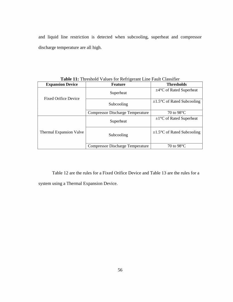
56
and liquid line restriction is detected when subcooling, superheat and compressor
discharge temperature are all high.
Table 11: Threshold Values for Refrigerant Line Fault Classifier
Expansion Device Feature Thresholds
Fixed Orifice Device
Superheat ±4°C of Rated Superheat
Subcooling ±1.5°C of Rated Subcooling
Compressor Discharge Temperature 70 to 98°C
Thermal Expansion Valve
Superheat ±1°C of Rated Superheat
Subcooling ±1.5°C of Rated Subcooling
Compressor Discharge Temperature 70 to 98°C
Table 12 are the rules for a Fixed Orifice Device and Table 13 are the rules for a
system using a Thermal Expansion Device.

57
Table 12: Rules for Refrigerant Line Fault Classifer (FXO valve)
SC condition SH Condition TCRI Condition Fault Detected
SC high
SH high - LLR
SH normal TCRI high LLR
TCRI normal Overcharge
SH low - Overcharge
SC normal SH high TCRI high LLR
TCRI normal Undercharge
SC low SH high - Undercharge
Table 13: Rules for Refrigerant Line Fault Classifer (TXV valve)
SC condition SH Condition TCRI Condition Fault Detected
SC high
SH high - LLR
SH normal TCRI high LLR
TCRI normal Overcharge
SC normal SH high TCRI high LLR
SC low SH high - Undercharge
SH normal TCRI normal Undercharge
Fouling Fault Detection Classifier
Input: dTCA, CS, dTEA, ES, SEER rating of the system, Presence of Undercharge,
Overcharge, or Liquid Line Restriction.
Output: Presence of Condenser and Evaporator Fouling.
After knowledge of any possible charging or refrigerant line faults, the next step
is to detect any possible fouling faults. The threshold value for the CS and dTCA depends
on the efficiency of the air conditioning system or its SEER rating. Higher efficiency
units have more condenser coils, thus the temperature difference between the saturated
condenser temperature and the ambient air temperature or the Condenser Split can be

58
lower. Since the saturated temperature and pressure can be lower for higher SEER rated
units, lesser heat needs to be rejected. Therefore the temperature difference of the
condenser inlet and outlet air is also lower. The thresholds used by the Fouling Fault
Detection Classifier are summarized in Table 14.
Table 14: Thresholds used by the Fouling Fault Detection Classifier
Feature Thresholds
Condenser Split
For SEER >13, 8±2°C
for SEER= 11 or 12, 10±2°C
and for SEER < 10, 14±2°C
Evaporator Split 18 to 25°C
Temperature difference of air across Condenser
For SEER >13, 4 to 6°C
for SEER= 11 or 12, 8 to 11°C
and for SEER < 10, 12 to 15°C
Temperature difference of air across Evaporator 10 to 16°C
The rules for detecting the fouling faults vary based on the presence or absence
of charge and refrigerant line faults. In general, condenser fouling is detected when both
the condenser air temperature difference and the condenser split are high. Evaporator
fouling is detected when the evaporator air temperature difference is low and the
evaporator split is high. To prevent any incorrect diagnosis, this classifier also makes use
of user prompts to verify the presence of evaporator and condenser fouling.
The rules used to detect fouling faults are summarized in Table 15. Since like
Evaporator Fouling, Refrigerant Undercharge and Liquid Line Restriction faults also
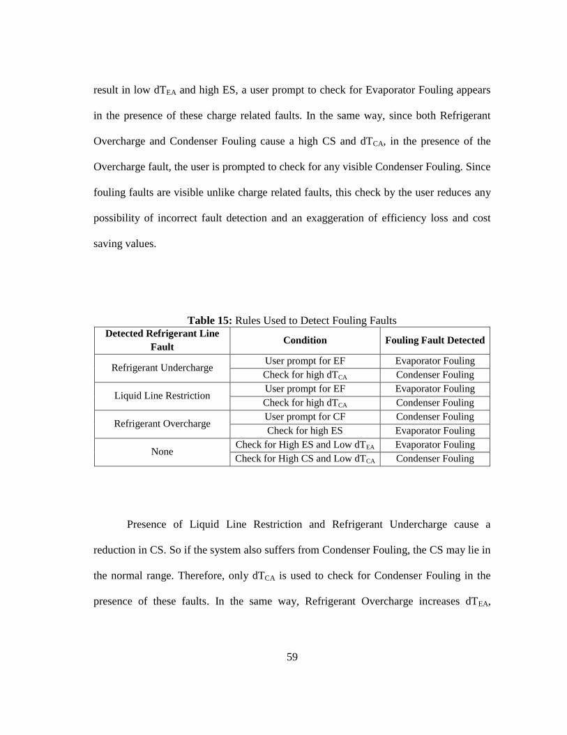
59
result in low dTEA and high ES, a user prompt to check for Evaporator Fouling appears
in the presence of these charge related faults. In the same way, since both Refrigerant
Overcharge and Condenser Fouling cause a high CS and dTCA, in the presence of the
Overcharge fault, the user is prompted to check for any visible Condenser Fouling. Since
fouling faults are visible unlike charge related faults, this check by the user reduces any
possibility of incorrect fault detection and an exaggeration of efficiency loss and cost
saving values.
Table 15: Rules Used to Detect Fouling Faults
Detected Refrigerant Line
Fault Condition Fouling Fault Detected
Refrigerant Undercharge User prompt for EF Evaporator Fouling
Check for high dTCA Condenser Fouling
Liquid Line Restriction User prompt for EF Evaporator Fouling
Check for high dTCA Condenser Fouling
Refrigerant Overcharge User prompt for CF Condenser Fouling
Check for high ES Evaporator Fouling
None Check for High ES and Low dTEA Evaporator Fouling
Check for High CS and Low dTCA Condenser Fouling
Presence of Liquid Line Restriction and Refrigerant Undercharge cause a
reduction in CS. So if the system also suffers from Condenser Fouling, the CS may lie in
the normal range. Therefore, only dTCA is used to check for Condenser Fouling in the
presence of these faults. In the same way, Refrigerant Overcharge increases dTEA,

60
therefore to detect Evaporator Fouling in presence of this fault only ES is used.
Fault Evaluation
Once a fault is detected, the fault must evaluated to know if the benefit of
repairing the fault will justify its expense. This involves three things- predicting the level
of fault, predicting the efficiency loss due to the fault, and finally calculating the
corresponding cost saving and the payback for repairing the fault.
Refrigerant Undercharge and Overcharge
Input: SC, Rated Subcooling, SH, Rated Superheat, Presence of Accumulator, Type of
Expansion Device, Type of Refrigerant
Output: Predicted Percent Incorrect Charge and Predicted Loss of EER
The device can predict the percentage overcharge and undercharge by using a
virtual refrigerant charge sensor. The sensor uses actual values of subcooling and
superheat, with rated values of subcooling and superheat to estimate the amount of
incorrect charge in the system. It also uses a few constants like Ksc-sh , Kch, ,Xhs,rated and αo
whose values would ideally depend on the type of expansion valve, type of system and
the size of the system. However tests comparing the use of experimentally determined
parameters and default parameters showed that for the purposes of the device, the default
parameters could be used [35]. Xhs,rated, is the ratio of high side refrigerant charge to the
total refrigerant charge, and αo which is the ratio of the refrigerant charge necessary to
have saturated liquid at the exit of the condenser to the rated refrigerant charge. Ksc-sh is

61
a constant calculated using rated subcooling and superheat with the subcooling and
superheat measured at some other operating condition.
After conducting several tests by changing the operating conditions and the
expansion valve, the default values for all constants were assumed as follows: αo is 0.75
and Xhs,rated is 0.73 for all systems, and. Ksc-sh could be averaged to 1/2.5.
The results for the differences in default and actual parameter values showed that
the error for TXV systems ranged from -8% to 7% and for FXO systems ranged from -
15% to 6%. The error increased with increasing amount of undercharge and overcharge.
For the purposes of the low cost device, these errors were acceptable. After confirming
these parameter values, the following equations can be used to predict the level incorrect
charge.
Percent Incorrect Charge = {1
Kch
[SC − SCrated] − [(Ksc−sh)(SH − SHrated)]} × 100
where, Kch =SCrated
(1 −∝o)(Xhs)
and ∝o= 0.75, Xhs = 0.73 and Ksc−sh = 0.4
The sensor ignores the amount of charge held per unit length in the refrigerant
tubing running between indoor and outdoor units and is thus not as accurate. It also does
not work well at higher levels of under- and overcharge. Nevertheless, it still provides a
rough estimate of percent overcharge or undercharge that is sufficient for auditing
purposes. The corresponding efficiency loss due to the predicted amount of incorrect
charge is calculated by referring to tests conducted by researchers to quantify the related
loss in EER.

62
Undercharge – EER loss
Input: Percent Undercharge, Type of Expansion Device, Type of Refrigerant, Presence
of Accumulator
Output: Percent loss in EER
Tests done by Kim and Braun (2010) [11] that recorded the effect of undercharge
on the efficiency of air conditioning systems using different expansion devices (TXV or
FXO) and different refrigerants (R22 or R410A) were used to develop a linear
relationship between percent level of undercharge and the related EER loss.
Percent EER Loss = (100 − %underchage)(A) + B
For a fixed orifice device, the constants A and B changed based on the absence
and presence of an accumulator. For a thermal expansion device, the constants changed
based on the type of refrigerant (Table 16).
Table 16: Constants used in Equation to predict EER Loss due to Undercharge Fixed Orifice, Accumulator A= -0.5558 and B=56.256
Fixed Orifice, No Accumulator A= -0.6833 and B=66.53
TXV, R410A A= 0.9198 and B=88.868
TXV, R22 A= -0.6962 and B=70.708
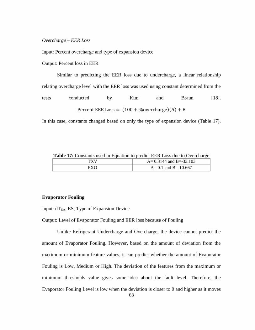
63
Overcharge – EER Loss
Input: Percent overcharge and type of expansion device
Output: Percent loss in EER
Similar to predicting the EER loss due to undercharge, a linear relationship
relating overcharge level with the EER loss was used using constant determined from the
tests conducted by Kim and Braun [18].
Percent EER Loss = (100 + %overcharge)(A) + B
In this case, constants changed based on only the type of expansion device (Table 17).
Table 17: Constants used in Equation to predict EER Loss due to Overcharge
TXV A= 0.3144 and B=-33.103
FXO A= 0.1 and B=-10.667
Evaporator Fouling
Input: dTEA, ES, Type of Expansion Device
Output: Level of Evaporator Fouling and EER loss because of Fouling
Unlike Refrigerant Undercharge and Overcharge, the device cannot predict the
amount of Evaporator Fouling. However, based on the amount of deviation from the
maximum or minimum feature values, it can predict whether the amount of Evaporator
Fouling is Low, Medium or High. The deviation of the features from the maximum or
minimum thresholds value gives some idea about the fault level. Therefore, the
Evaporator Fouling Level is low when the deviation is closer to 0 and higher as it moves

64
away from 0 to this maximum value.
|(20℃ − ES)| + |(dTEA − 10℃)| = Evaporator Fouling Level
The device can predict the maximum and minimum amount of EER loss due to
evaporator fouling based on the type of expansion device. Tests were done by
Watt(1997)[36] to estimate the amount of efficiency loss due to evaporator fouling in a
TXV and FXO system. The results from these tests were used in the device.
Table 18: Maximum and Minimum EER Loss due to Evaporator Fouling
TXV Maximum EER Loss= 7%
Minimum EER Loss=1%
FXO Maximum EER Loss= 10%
Minimum EER Loss=5%
Condenser Fouling
Input: dTCA, CS, Type of Expansion Device
Output: Level of Condenser Fouling and EER loss because of Fouling
Like Evaporator Fouling, in case of Condenser Fouling, the device bases the
amount of Condenser Fouling on the amount of deviation from the maximum CS and
dTCA values. Therefore, the Condenser Fouling Level is low when the deviation is closer
to 0 and higher as it moves away from 0 to this maximum value.
|(6℃ − dTCA)| + |(10℃ − CS)| = Condenser Fouling Level

65
The device predicts the maximum and minimum amount of EER loss due to condenser
fouling based on the type of expansion device. Results from the tests done by
Watt(1997) [36] were used to estimate the maximum and minimum EER loss (Table 19).
Table 19: Maximum and Minimum EER Loss due to Condenser Fouling
TXV Maximum Loss= 15%
Minimum Loss=5%
FXO Maximum Loss= 30%
Minimum Loss=5%
Liquid Line Restriction
Input: Rated Subcooling and Superheat, Actual Subcooling and Superheat
Output: Level of Liquid Line Restriction and EER Loss due to Liquid Line Restriction
The level of liquid line restriction using non-invasive temperature and pressure
measurements cannot be predicted with certainty. Instead, like the fouling faults, the
deviation from the expected feature values is used to classify the level of the fault as
low, medium or high. The expected values of SC and SH are nothing but the rated values
of SC and SH. Therefore, the fault level is Low when this value is closer to 0 and High
as it moves towards the maximum deviation value.
|(Rated SH − SH)| + |(Rated SC − SC)| + |(TCRI − 71℃)|
= Liquid Line Restriction Level

66
The maximum and minimum EER loss due a restricted liquid line is based on
tests conducted by Braun[8] for different amounts of pressure difference across the
valve.
Minimum EER loss= 3%
Maximum EER loss=9%
Estimating the Cost Savings
Input: Capacity of the Unit, SEER rating, Operating Hours, Cost of Electrical Energy
and Maximum and Minimum Percent EER loss due to the Faults
Output: Current Operating Cost, Proposed Operating Cost and Cost Savings.
The operating cost is calculated using the nameplate SEER rating, cooling
capacity and operating hours of the system using the following formula-
Operating Cost
= (Capacity in BTU
hr⁄ )(Operating hours per year)(Cost of Electrical Energy )
(1000 WkW⁄ )(SEER rating)
All the parameters in the above formula remain the same, except the SEER rating
which decreases because of the presence of faults. Therefore, a maximum and minimum
SEER rating is calculated based on the product of the EER percent loss of the detected
faults.

67
Minimum Reduced EER %
= (Condenser Fouling LossMin)(Evaporator Fouling LossMin)(LLR LossMin)
(Loss due to Undercharge)(Loss due to Overcharge)
SEERMin = (Minimum Reduced EER%)(SEER)
Maximum Reduced EER %
= (Condenser Fouling LossMax)(Evaporator Fouling LossMax)(LLR LossMax)
(Loss due to Undercharge)(Loss due to Overcharge)
SEERMax = (Maximum Reduced EER%)(SEER)
The SEERMax and SEERMin are then used in the main SEER-cost equation to
calculate the actual maximum and minimum cost. The nameplate SEER rating is used to
calculate the proposed operating cost, and the difference between the actual and
proposed cost gives the cost savings.
68
CHAPTER VI
TESTS: INDIVIDUAL FAULTS AT TFCL
The proposed algorithm was initially tested in the Thermo-Fluids Controls
Laboratory by introducing the five faults individually to a 3-ton residential, split air
conditioning system. These tests helped in two ways: they confirmed the effect of each
fault on the 7 features, and helped realize the sensitivity of the algorithm to the 5 faults.
In this chapter, a description of the air conditioning system and the method of
introducing the faults in the system is discussed. The results of the tests follow.
System Description
The system used to test the algorithm of the device is a 3 ton, residential split
heat pump system donated by Trane. It is installed with an electronic expansion valve
from Parker. The system uses R410A refrigerant, and a two stage scroll compressor. The
placement of temperature sensors, pressure sensors, mass flow rate sensor, and humidity
sensors is shown in Figure 7, the parts are described in Table 20 and the user information
for the system is summarized in Table 21.
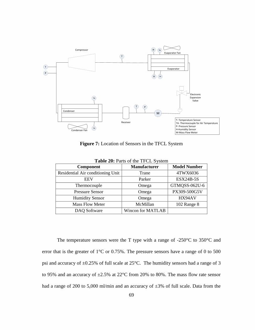
69
Compressor
Receiver
T
M
P
H
H
T
T
PTA
TA
TA
TA
Condenser
Evaporator
Evaporator Fan
Condenser Fan
Electronic Expansion
Valve
T- Temperature SensorTA- Thermocouple for Air TemperatureP- Pressure SensorH-Humidity SensorM-Mass Flow Meter
Figure 7: Location of Sensors in the TFCL System
Table 20: Parts of the TFCL System
Component Manufacturer Model Number
Residential Air conditioning Unit Trane 4TWX6036
EEV Parker ESX24B-5S
Thermocouple Omega GTMQSS-062U-6
Pressure Sensor Omega PX309-500G5V
Humidity Sensor Omega HX94AV
Mass Flow Meter McMillan 102 Range 8
DAQ Software Wincon for MATLAB
The temperature sensors were the T type with a range of -250°C to 350°C and
error that is the greater of 1°C or 0.75%. The pressure sensors have a range of 0 to 500
psi and accuracy of ±0.25% of full scale at 25°C. The humidity sensors had a range of 3
to 95% and an accuracy of ±2.5% at 22°C from 20% to 80%. The mass flow rate sensor
had a range of 200 to 5,000 ml/min and an accuracy of ±3% of full scale. Data from the

70
humidity and mass flow rate sensors is not used in the algorithm, but was recorded.
Therefore, the 7 temperature measurements and the 2 pressure measurements required
by the proposed algorithm were available. The user inputs- SEER rating, capacity of the
system and type of refrigerant was seen on the nameplate, and the rated subcooling was
obtained from the maintenance brochure. The rated superheat was set to 10°C by the
EEV that was controlled by a PID controller. A Simulink model was used to control the
working of the air conditioning system. The evaporator and condenser fan speed, the
compressor stage and the opening of the EEV could be controlled.
Table 21: User Inputs for the Laboratory Test System
User Input Value
1 Capacity of the System 36,000 BTU/h
2 Rated Subcooling 3.5°C
3 Rated Superheat 10°C
4 Type of expansion device in the system TXV
5 SEER Rating of the System 16
6 Type of Refrigerant Used R410A
7 Presence of accumulator in the system Yes
8 Avoided Cost of Electrical Energy $0.010
kWh
9 Hours of Operation per Year 8,760 hr
yr
Introducing Faults
Individual Faults were introduced to the system to-

71
To verify the effect of the individual faults on the 7 different features, thus
helping the development of the algorithm for multiple fault detection.
Check the basic fault detection and evaluation algorithm developed. Thus,
gaining an understanding of sensitivity of the algorithm, the chosen thresholds to
the various faults, the predicted level of charging faults, and the related
efficiency loss and cost savings.
The 5 faults that the device intends to detect were introduced in the system at
different levels as shown in Table 22.

72
Table 22: Method used to Introduce Faults in the Laboratory Test System
Fault Method of
simulating the
fault
Simulation
Parameter
Level
1
Level
2
Level
3
Level
4
Level
5
Condenser
Fouling
Covering the
condenser with
strips of paper.
% reduction in
the area of
condenser
exposed to heat
exchange
20% 40% 60% 80% 100%
Evaporator
Fouling
Covering the
evaporator coil
with strips of
paper
% reduction in
the area of
condenser
exposed to heat
exchange
20% 40% 60% 80% 100%
Refrigerant
Undercharge
Removing some
charge from the
system
% reduction in
the amount of
refrigerant in the
system
0% 9% 18% 28% 36%
Refrigerant
Overcharge
Adding
refrigerant to the
system
% increase in the
amount of
refrigerant
charge in the
system
0% 5% 10% 15% 20%
Liquid Line
Restriction
Restricting the
opening of the
electronic
expansion valve
by a fixed
amount
% increase in the
pressure
difference across
the restriction
0% 4% 11% 18% 24%
Results
Effect of Individual Faults on Features
The effect of the individual faults on the 7 features was analyzed to help the
development of a more robust multiple fault detection algorithm.

73
Subcooling
The rated subcooling of the system is about 3.5°C. As seen in Figure 8,
subcooling of the system is somewhat sensitive to all the 5 faults. However, the two
faults that affect it the most are refrigerant overcharge and undercharge. It also increases
with an increasing liquid line restriction as the fault causes some refrigerant to be backed
up in the condenser. However, excessive testing on the system had caused a leak in the
system, which was noticed towards the end when performing the tests for the liquid line
restriction fault. This caused the subcooling at no fault conditions to reduce to a lower
value. Therefore, when testing the algorithm for the liquid line restriction fault, the rated
subcooling value was reset to the value that was seen right before introducing the fault.
Therefore, an increase in subcooling is used to detect refrigerant overcharge and liquid
line restriction, and a decrease in subcooling is used to detect refrigerant undercharge.
As seen in the figure, subcooling isn’t affected as much by fouling faults.

74
Figure 8: Effect of Faults on Subcooling
Superheat
The rated superheat of the system is 10°C. Since the system uses an EEV which
keeps the superheat value constant as far as possible, Figure 9 shows an unchanging
value of superheat for condenser fouling, evaporator fouling and refrigerant overcharge.
However, when there is a lack of refrigerant, or a two-phase refrigerant entering the
EEV, it cannot function as well to keep the superheat constant. Therefore, superheat
increases for liquid line restriction and high levels for refrigerant undercharge.
1 2 3 4 5 0
1
2
3
4
5
6
7
Fault Level
Subcoolin
g (
Celc
ius)
Condenser Fouling
Evaporator Fouling
Liquid Line Restriction
Undercharge
Overcharge

75
Figure 9: Effect of Faults on Superheat
Compressor Discharge Temperature
The compressor discharge temperature for this system varies between 55°C to
71°C. It is sensitive to the load and operating conditions of the system unlike the other
features. However, it rises abnormally when there is a restricted liquid line. It also
increases with a fouled condenser or refrigerant undercharge at high levels. With suitable
thresholds, this feature can be used to detect liquid line restriction (Figure 10).
1 2 3 4 5 0
5
10
15
20
25
30
Fault Level
Superh
eat
(Celc
ius)
Condenser Fouling
Evaporator Fouling
Liquid Line Restriction
Undercharge
Overcharge
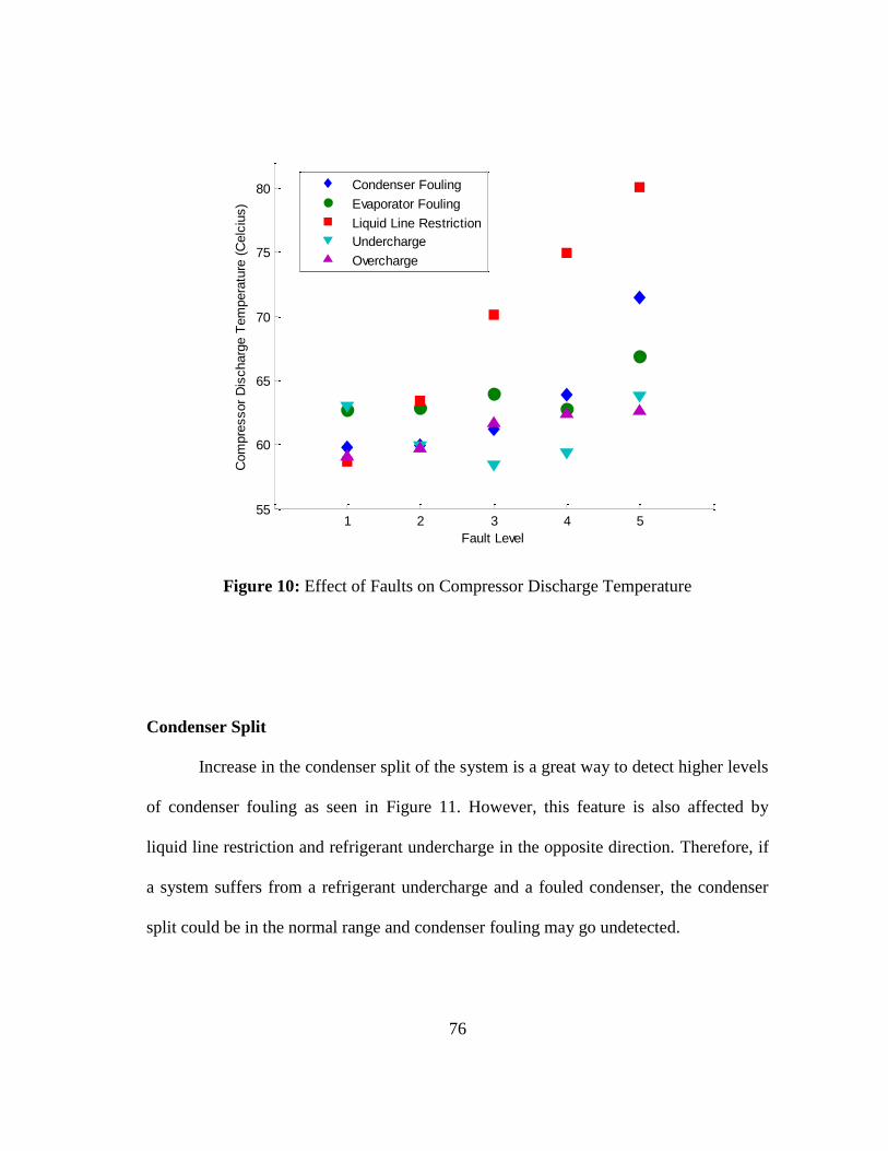
76
Figure 10: Effect of Faults on Compressor Discharge Temperature
Condenser Split
Increase in the condenser split of the system is a great way to detect higher levels
of condenser fouling as seen in Figure 11. However, this feature is also affected by
liquid line restriction and refrigerant undercharge in the opposite direction. Therefore, if
a system suffers from a refrigerant undercharge and a fouled condenser, the condenser
split could be in the normal range and condenser fouling may go undetected.
1 2 3 4 5 55
60
65
70
75
80
Fault Level
Com
pre
ssor
Dis
charg
e T
em
pera
ture
(C
elc
ius)
Condenser Fouling
Evaporator Fouling
Liquid Line Restriction
Undercharge
Overcharge
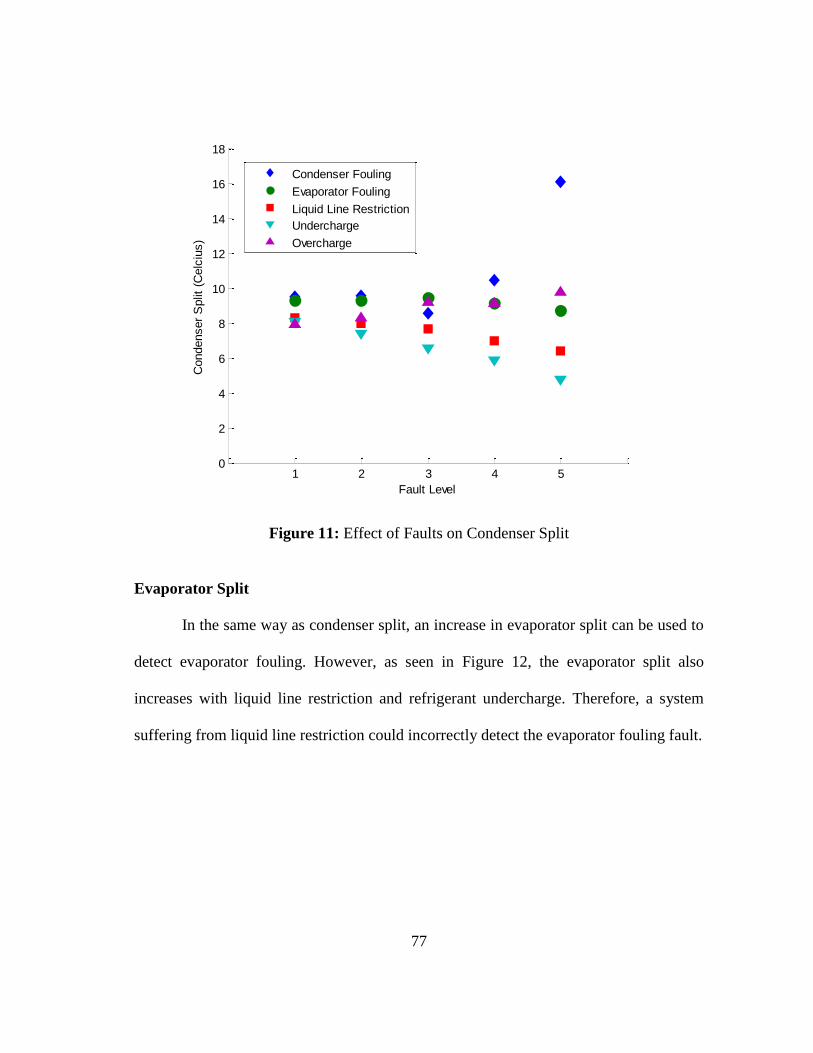
77
Figure 11: Effect of Faults on Condenser Split
Evaporator Split
In the same way as condenser split, an increase in evaporator split can be used to
detect evaporator fouling. However, as seen in Figure 12, the evaporator split also
increases with liquid line restriction and refrigerant undercharge. Therefore, a system
suffering from liquid line restriction could incorrectly detect the evaporator fouling fault.
1 2 3 4 5 0
2
4
6
8
10
12
14
16
18
Fault Level
Condenser
Split
(C
elc
ius)
Condenser Fouling
Evaporator Fouling
Liquid Line Restriction
Undercharge
Overcharge
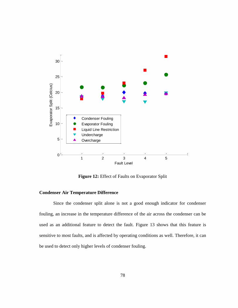
78
Figure 12: Effect of Faults on Evaporator Split
Condenser Air Temperature Difference
Since the condenser split alone is not a good enough indicator for condenser
fouling, an increase in the temperature difference of the air across the condenser can be
used as an additional feature to detect the fault. Figure 13 shows that this feature is
sensitive to most faults, and is affected by operating conditions as well. Therefore, it can
be used to detect only higher levels of condenser fouling.
1 2 3 4 5 0
5
10
15
20
25
30
Fault Level
Evapora
tor
Split
(C
elc
ius)
Condenser Fouling
Evaporator Fouling
Liquid Line Restriction
Undercharge
Overcharge
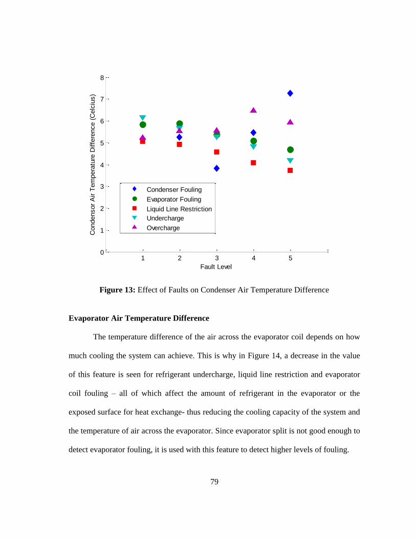
79
Figure 13: Effect of Faults on Condenser Air Temperature Difference
Evaporator Air Temperature Difference
The temperature difference of the air across the evaporator coil depends on how
much cooling the system can achieve. This is why in Figure 14, a decrease in the value
of this feature is seen for refrigerant undercharge, liquid line restriction and evaporator
coil fouling – all of which affect the amount of refrigerant in the evaporator or the
exposed surface for heat exchange- thus reducing the cooling capacity of the system and
the temperature of air across the evaporator. Since evaporator split is not good enough to
detect evaporator fouling, it is used with this feature to detect higher levels of fouling.
1 2 3 4 5 0
1
2
3
4
5
6
7
8
Fault Level
Condensor
Air T
em
pera
ture
Diffe
rence (
Celc
ius)
Condenser Fouling
Evaporator Fouling
Liquid Line Restriction
Undercharge
Overcharge

80
Figure 14: Effect of Faults on Evaporator Air Temperature Difference
Fault Detection and Evaluation for Individual Faults
The results of the tests for individual faults is shown in Table 23. It was realized
that the algorithm is not very sensitive to the fouling faults, which are detected at a level
only higher than 80%. In contrast, charge related faults and refrigerant line faults are
detected at low levels. There were two instances of incorrect fault detection; Liquid Line
Restriction at higher levels was incorrectly detected as Evaporator Fouling. This is
because both faults have the same effect on dTEA and ES, and the increase in the SC, SH
and TCRI that is normally caused by Liquid Line Restriction was within the thresholds.
1 2 3 4 5 0
2
4
6
8
10
12
14
Fault Level
Evapora
tor
Air T
em
pera
ture
Diffe
rence (
Celc
ius)
Condenser Fouling
Evaporator Fouling
Liquid Line Restriction
Undercharge
Overcharge

81
This could have been improved if the thresholds were tighter, but it could have led to
incorrect fault detection of other faults.
Table 23: Results of Tests for Individual Faults
Fault Fault Levels
Introduced
Level First
Detected
Predicted
Efficiency Loss
Predicted Annual
Cost Savings Per
Ton
Refrigerant
Undercharge 9 to 36% 9% 6 to 14% $37 to $105
Refrigerant
Overcharge 5 to 20% 10% 1 to 2% $3 to $12
Liquid Line
Restriction 3 to 24% 11% 3 to 9% $20 to $64
Condenser
Fouling 20 to 100% 100% 5 to 15% $34 to $116
Evaporator
Fouling 20 to 100% 100% 1 to 7% $6 to $49
Predict Incorrect Charge Level
Since fault levels could be predicted for only refrigerant undercharge and
overcharge, Figure 15 and Figure 16 show how the actual incorrect charge level
compares to the level predicted by the device. Since the virtual charge sensor makes
many assumptions, it was known that the sensor would not be able to accurately detect
the level of under- or overcharge. According to the results, it was learned that the
inaccuracy did not lead to overestimation of the incorrect charge level. This would
prevent energy auditors from over-estimating the efficiency loss, and help them predict
realistic cost savings.

82
Figure 15: Actual and Predicted Refrigerant Charge for an Undercharged System
Figure 16: Actual and Predicted Refrigerant Charge for an Overcharged System
1 2 3 4 50
5
10
15
20
25
30
35
40
Fault Level
Underc
harg
e L
evel (%
)
Actual Undercharge Level
Predicted Undercharge Level
1 2 3 4 50
5
10
15
20
25
Fault Level
Overc
harg
e L
evel (%
)
Actual Overcharge Level
Predicted Overcharge Level

83
Thus, the effect of the different faults on the features helped verify the chosen thresholds
and the rules for the proposed device. The sensitivity of the device to these faults was
also recorded in these tests. As the next step, the device would be tested with a second
set of data to check its sensitivity and working with a different system. The following
chapter discusses the results from testing the algorithm with a set of data generated at the
Energy Systems Laboratory.

84
CHAPTER VII
INDIVIDUAL FAULT TESTS AT ESL
The proposed algorithm was also tested against a second set of data, to verify its
thresholds and validate the method. This dataset was generated at the Energy Systems
Laboratory by Mr. James Watt for his tests used to identify temperature-based indicators
that, together with one return-air humidity point, could detect performance deterioration
resulting from equipment or system degradation [36].
System and Fault Description
For these tests, a split-system direct-expansion air conditioner was used, with the
air-conditioner test bench equipped with the choice of either using a short-tube orifice
(STO) or a thermal expansion valve (TXV). The degraded conditions studied included
low evaporator airflow, high- and low-charge, and a blocked condenser coil. These
degraded conditions have the same effect on the system as the evaporator filter fouling,
refrigerant overcharge, refrigerant undercharge and condenser fouling faults
respectively.
Table 24 shows how the degraded condition or the fault was simulated, the fault
levels introduced and the number of tests for each expansion device.
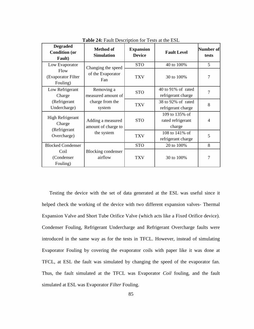
85
Table 24: Fault Description for Tests at the ESL
Degraded
Condition (or
Fault)
Method of
Simulation
Expansion
Device Fault Level
Number of
tests
Low Evaporator
Flow
(Evaporator Filter
Fouling)
Changing the speed
of the Evaporator
Fan
STO 40 to 100% 5
TXV 30 to 100% 7
Low Refrigerant
Charge
(Refrigerant
Undercharge)
Removing a
measured amount of
charge from the
system
STO 40 to 91% of rated
refrigerant charge 7
TXV 38 to 92% of rated
refrigerant charge 8
High Refrigerant
Charge
(Refrigerant
Overcharge)
Adding a measured
amount of charge to
the system
STO
109 to 135% of
rated refrigerant
charge
4
TXV 108 to 141% of
refrigerant charge 5
Blocked Condenser
Coil
(Condenser
Fouling)
Blocking condenser
airflow
STO 20 to 100% 8
TXV 30 to 100% 7
Testing the device with the set of data generated at the ESL was useful since it
helped check the working of the device with two different expansion valves- Thermal
Expansion Valve and Short Tube Orifice Valve (which acts like a Fixed Orifice device).
Condenser Fouling, Refrigerant Undercharge and Refrigerant Overcharge faults were
introduced in the same way as for the tests in TFCL. However, instead of simulating
Evaporator Fouling by covering the evaporator coils with paper like it was done at
TFCL, at ESL the fault was simulated by changing the speed of the evaporator fan.
Thus, the fault simulated at the TFCL was Evaporator Coil fouling, and the fault
simulated at ESL was Evaporator Filter Fouling.

86
Evaporator Coil Fouling causes reduction in cooling capacity due to lesser
surface area for heat exchange, thus the temperature of air across the evaporator
(dTEA) decreases.
In case of evaporator filter fouling, the loss in cooling capacity is due to lesser air
entering the system due to the restricted filter. Therefore, the small quantity of air
that does enter the evaporator gets overcooled which causes the temperature
difference of air across the evaporator (dTEA) in case of Evaporator Filter Fouling
to increase.
Thus, the device was modified to detect a sixth fault- Evaporator Filter Fouling .The
only difference in the detection algorithm was that Evaporator Coil Fouling was detected
when dTEA was below the threshold and Evaporator Filter Fouling was detected when
dTEA was above the threshold value.
Results
As seen in Table 25, sensitivity of the device to faults for both expansion devices
was almost the same. For the fouling faults, the device worked better on the ESL system
than the TFCL system. However, in case of Condenser Fouling it also incorrectly
detected Refrigerant Undercharge at higher levels of the fault. This was because in the
condenser fouling tests, the subcooling of the system decreased with increasing levels of
fouling. Another instance of incorrect fault detection was detecting evaporator coil
fouling for overcharge at the highest level for the TXV system. This was because the
high overcharge caused the dTEA to decrease beyond its lower threshold.
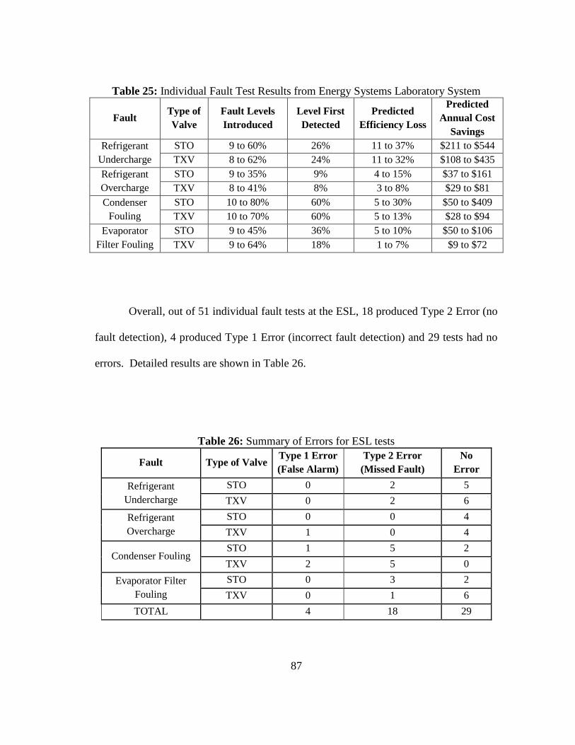
87
Table 25: Individual Fault Test Results from Energy Systems Laboratory System
Fault Type of
Valve
Fault Levels
Introduced
Level First
Detected
Predicted
Efficiency Loss
Predicted
Annual Cost
Savings
Refrigerant
Undercharge
STO 9 to 60% 26% 11 to 37% $211 to $544
TXV 8 to 62% 24% 11 to 32% $108 to $435
Refrigerant
Overcharge
STO 9 to 35% 9% 4 to 15% $37 to $161
TXV 8 to 41% 8% 3 to 8% $29 to $81
Condenser
Fouling
STO 10 to 80% 60% 5 to 30% $50 to $409
TXV 10 to 70% 60% 5 to 13% $28 to $94
Evaporator
Filter Fouling
STO 9 to 45% 36% 5 to 10% $50 to $106
TXV 9 to 64% 18% 1 to 7% $9 to $72
Overall, out of 51 individual fault tests at the ESL, 18 produced Type 2 Error (no
fault detection), 4 produced Type 1 Error (incorrect fault detection) and 29 tests had no
errors. Detailed results are shown in Table 26.
Table 26: Summary of Errors for ESL tests
Fault Type of Valve Type 1 Error
(False Alarm)
Type 2 Error
(Missed Fault)
No
Error
Refrigerant
Undercharge
STO 0 2 5
TXV 0 2 6
Refrigerant
Overcharge
STO 0 0 4
TXV 1 0 4
Condenser Fouling STO 1 5 2
TXV 2 5 0
Evaporator Filter
Fouling
STO 0 3 2
TXV 0 1 6
TOTAL
4 18 29

88
Predicting Incorrect Charge Level
The working of the virtual charge sensor that predicts the incorrect charge level
was checked with the different types of valves used in the ESL tests. Figure 17 and
Figure 18 show the results of charge level prediction for undercharge and overcharge
faults with the STO valve. It is seen that the sensor very rarely overestimates the level of
the fault in case of undercharge. However, for the overcharge fault, the level of the fault
is overestimated for the STO valve.
Figure 17: Undercharge Fault Level Prediction for STO valve
1 2 3 4 5 6 7 80
10
20
30
40
50
60
70
Fault Level
Underc
harg
e L
evel (%
)
Actual Undercharge Level
Predicted Undercharge Level

89
Figure 18: Overcharge Fault Level Prediction for STO valve
Figure 19 and Figure 20 show the results of charge level prediction for
undercharge and overcharge faults with the TXV valve. It is seen that the sensor works
better for the TXV valve. It very rarely over-estimates the incorrect charge level except
for a few instances in the overcharge fault tests.
1 2 3 4 5 60
10
20
30
40
50
60
Fault Level
Overc
harg
e L
evel (%
)
Actual Overcharge Level
Predicted Overcharge Level

90
Figure 19: Undercharge Fault Level Prediction for TXV valve
Figure 20: Overcharge Fault Level Prediction for TXV valve
According to the results, it can be said that the device worked better when
detecting Evaporator Filter Fouling and predicting the level of incorrect charge for the
1 2 3 4 5 6 7 8 90
10
20
30
40
50
60
70
Fault Level
Underc
harg
e L
evel (%
)
Actual Undercharge Level
Predicted Undercharge Level
1 2 3 4 5 6 70
5
10
15
20
25
30
35
40
45
Fault Level
Overc
harg
e L
evel (%
)
Actual Overcharge Level
Predicted Overcharge Level
91
thermal expansion valve tests, but in general, it performed well for both expansion
devices.

92
CHAPTER VIII
MULTIPLE FAULT TESTS AT TFCL
After testing the device for individual faults, multiple faults were introduced to
the TFCL air conditioner. In these set of tests, two faults were introduced at a time; a
fouling fault with a refrigerant line fault. The level of the refrigerant line fault was
varied, and both the fouling faults were introduced at two levels- 40% and 80%.
Therefore, each combination had 4*2 = 8 tests.
Table 27: Fault Combinations Introduced for Multiple Fault Detection Tests
Refrigerant Line Fault Levels Introduced Fouling Fault Levels Introduced
Refrigerant Overcharge 11 to 35% Condenser Fouling 40% and 80%
Refrigerant Overcharge 11 to 35% Evaporator Fouling 40% and 80%
Refrigerant Undercharge 5 to 20% Condenser Fouling 40% and 80%
Refrigerant Undercharge 5 to 20% Evaporator Fouling 40% and 80%
Liquid Line Restriction 10 to 32% Condenser Fouling 40% and 80%
Liquid Line Restriction 10 to 32% Evaporator Fouling 40% and 80%
In addition to the fault combinations listed in Table 27, both evaporator and
condenser fouling fault were also introduced together at 5 different levels from 20 to
100% (5*5= 25 tests).
The results of multiple fault detection, and fault evaluation is discussed in this
chapter.

93
Refrigerant Undercharge
With Condenser Fouling
For this combination of faults, refrigerant undercharge was not detected in 3 of
the 8 tests (Figure 21). For the remaining tests, both faults were detected at low levels of
undercharge and high levels of condenser fouling. This is because high refrigerant
undercharge negates the increase of condenser split caused by condenser fouling. A
check for high dTCA is done in the presence of undercharge to check for condenser
fouling.
Figure 21: Results for tests on Undercharge and Condenser Fouling
0 5 10 15 20 25 30 35 400
20
40
60
80
100
Undercharge Level (%)
Condenser
Foulin
g L
evel (%
)
Both Detected
Undercharge Detected
None Detected

94
With Evaporator Fouling
Out of the 8 tests, neither of the two faults in this combination are detected in 5
tests (Figure 22). However, in the remaining tests, after an undercharge is detected, the
user is prompted to verify evaporator fouling as the symptoms of both faults are similar.
Therefore assuming the user can see the fouled evaporator, both faults are detected in the
remaining 3 of the 8 tests.
Figure 22: Results for tests on Undercharge and Evaporator Fouling
0 5 10 15 20 25 30 35 400
20
40
60
80
100
Undercharge Level (%)
Evapora
tor
Foulin
g L
evel (%
)
Both Detected
None Detected

95
Refrigerant Overcharge
With Condenser Fouling
Just like the evaporator fouling with undercharge combination, in case of
condenser fouling with overcharge, the user is prompted to check for condenser fouling
in the presence of an overcharge. This is because both faults cause an increase in CS and
dTCA. Assuming that the user can view the fouling on the condenser, 7 of 8 tests show
successful fault detection (Figure 23).
Figure 23: Results for tests on Overcharge and Condenser Fouling
0 5 10 15 20 250
20
40
60
80
100
Overcharge Level (%)
Condenser
Foulin
g L
evel (%
)
Both Detected
None Detected
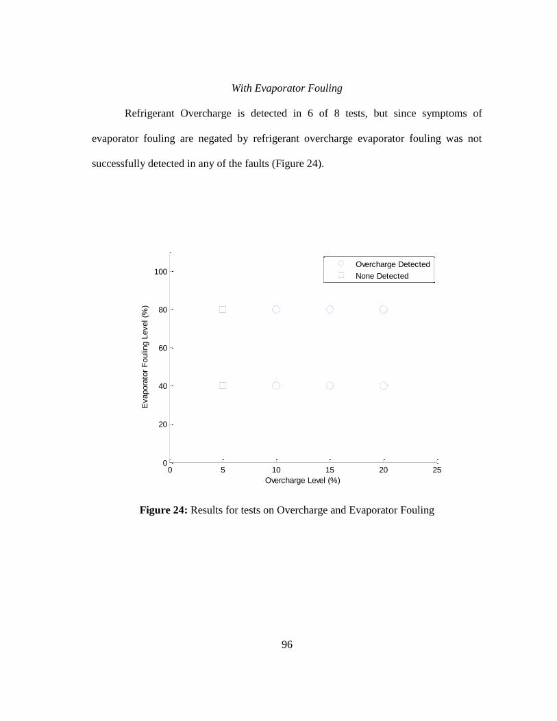
96
With Evaporator Fouling
Refrigerant Overcharge is detected in 6 of 8 tests, but since symptoms of
evaporator fouling are negated by refrigerant overcharge evaporator fouling was not
successfully detected in any of the faults (Figure 24).
Figure 24: Results for tests on Overcharge and Evaporator Fouling
0 5 10 15 20 250
20
40
60
80
100
Overcharge Level (%)
Evapora
tor
Foulin
g L
evel (%
)
Overcharge Detected
None Detected

97
Liquid Line Restriction
With Condenser Fouling
In 5 of 8 tests for this combination LLR is detected, but condenser fouling is
detected in only 1 test. This is because the effect of the features used to detect fouling is
negated by high levels of LLR. There is one instance of incorrect fault detection in the
test (Figure 25).
Figure 25: Results for tests on Liquid Line Restriction and Condenser Fouling
0 5 10 15 20 25 30 350
20
40
60
80
100
Liquid Line Restriction Level (%)
Condenser
Foulin
g L
evel (%
)
Both Detected
LLR Detected
None Detected
Incorrect Detection

98
With Evaporator Fouling
For this combination, evaporator fouling was detected in 6 of 8 tests. LLR was
detected in 4 of these tests (Figure 26). A user prompt was used to verify evaporator
fouling in these 4 tests.
Figure 26: Results for tests on Liquid Line Restriction and Evaporator Fouling
0 5 10 15 20 25 30 350
20
40
60
80
100
Liquid Line Restriction Level (%)
Evapora
tor
Foulin
g L
evel (%
)
Both Detected
Evaporator Fouling Detected
None Detected

99
Evaporator and Condenser Fouling
As is can be seen in Figure 27, both evaporator and condenser fouling were
successfully detected only at the maximum fault levels. In general, the faults were
detected at levels higher than 80%.
Figure 27: Results for tests on Evaporator and Condenser Fouling
0 20 40 60 80 1000
20
40
60
80
100
Evaporator Fouling Level (%)
Condenser
Foulin
g L
evel (%
)
Both Detected
Evaporator Fouling Detected
Condenser Fouling Detected
None Detected

100
Out of a total of 73 tests of multiple fault detection, 1 test detected a fault that
was not present in the system (Type 1 Error), in 26 tests none of the two faults were
detected (Type 2 Error: Both Faults), and 27 tests had incomplete fault detection where
only one of two faults were detected (Type 2 Error: One Fault). Successful multiple fault
detection occurred in 18 tests. Thus, at least one of the two faults were detected in over
60% of the tests with minimal instances of incorrect fault detection (Table 28).
Table 28: Summary of Errors for Multiple Fault Test Results from TFCL
Fault Combinations Type 1 Error
(False Alarm)
Type 2 Error
(Missed Fault):
Both Faults
Type 2 Error
(Missed Fault):
One Fault
No
Error
Refrigerant Undercharge
and Condenser Fouling 0 4 2 2
Refrigerant Undercharge
and Evaporator Fouling 0 5 0 3
Refrigerant Overcharge
and Condenser Fouling 0 1 0 7
Refrigerant Overcharge
and Evaporator Fouling 0 2 6 0
LLR and Condenser
Fouling 1 2 4 1
LLR and Evaporator
Fouling 0 2 2 4
Evaporator and
Condenser Fouling 0 10 13 1
TOTAL 1 26 27 18

101
Fault Evaluation for Multiple Faults
Table 29 shows a summary of the Fault Evaluation results of the Multiple Fault
Tests. The level of the fault, the range of total efficiency loss and cost savings related to
the fault combination is predicted. The device can predict the level of the refrigerant line
fault (Fault 1) better than the fouling fault (Fault 2). Therefore, based on the level of the
fouling fault visible to the user, the total efficiency loss and cost savings can be
estimated from the maximum and minimum values predicted by the device.
Table 29: Summary of Fault Evaluation Results for Multiple Fault Tests
Fault 1 Level
Predicted Fault 2
Level
Predicted
Efficiency Loss
Predicted
Predicted
Cost
Savings
11%
Undercharge 9%
40% Evap
Fouling High 7 to 13% $46 to $92
11%
Undercharge 9%
80% Evap
Fouling Medium 7 to 13% $48 to $94
20%
Undercharge
Not
detected
40% Evap
Fouling
Not
detected 0% No savings
20%
Undercharge 10%
80% Evap
Fouling High 8 to 13% $50 to $96
30%
Undercharge
Not
detected
40% Evap
Fouling
Not
detected 0% No savings
30%
Undercharge
Not
detected
80% Evap
Fouling
Not
detected 0% No savings
35%
Undercharge
Not
detected
40% Evap
Fouling
Not
detected 0% No savings
35%
Undercharge
Not
detected
80% Evap
Fouling
Not
detected 0% No savings
11%
Undercharge 8%
40% Cond
Fouling
Not
detected 6% $37

102
Table 29: (Continued)
Fault 1 Level
Predicted Fault 2
Level
Predicted
Efficiency Loss
Predicted
Predicted
Cost
Savings
11%
Undercharge 9%
80% Cond
Fouling Low 11 to 20%
$76 to
$163
20%
Undercharge
Not
detected
40% Cond
Fouling
Not
detected 0%
No
savings
20%
Undercharge 8%
80% Cond
Fouling Low 10 to 20%
$69 to
$155
30%
Undercharge 11%
40% Cond
Fouling
Not
detected 7% $48
30%
Undercharge
Not
detected
80% Cond
Fouling
Not
detected 0%
No
savings
35%
Undercharge
Not
detected
40% Cond
Fouling
Not
detected 0%
No
savings
35%
Undercharge
Not
detected
80% Cond
Fouling
Not
detected 0%
No
savings
5%
Overcharge
Not
detected
40% Evap
Fouling
Not
detected 0%
No
savings
5%
Overcharge
Not
detected
80% Evap
Fouling
Not
detected 0%
No
savings
10%
Overcharge 9%
40% Evap
Fouling
Not
detected 2% $8
10%
Overcharge 8%
80% Evap
Fouling
Not
detected 2% $6
15%
Overcharge 7%
40% Evap
Fouling
Not
detected 1% $4
15%
Overcharge 7%
80% Evap
Fouling
Not
detected 1% $3
20%
Overcharge 10%
40% Evap
Fouling
Not
detected 2% $10
20%
Overcharge 10%
80% Evap
Fouling
Not
detected 2% $9
5%
Overcharge
Not
detected
40% Cond
Fouling
Not
detected 0%
No
savings
5%
Overcharge 8%
80% Cond
Fouling Low 6 to 16%
$40 to
$122
10%
Overcharge 9%
40% Cond
Fouling Low 7 to 17%
$44 to
$126
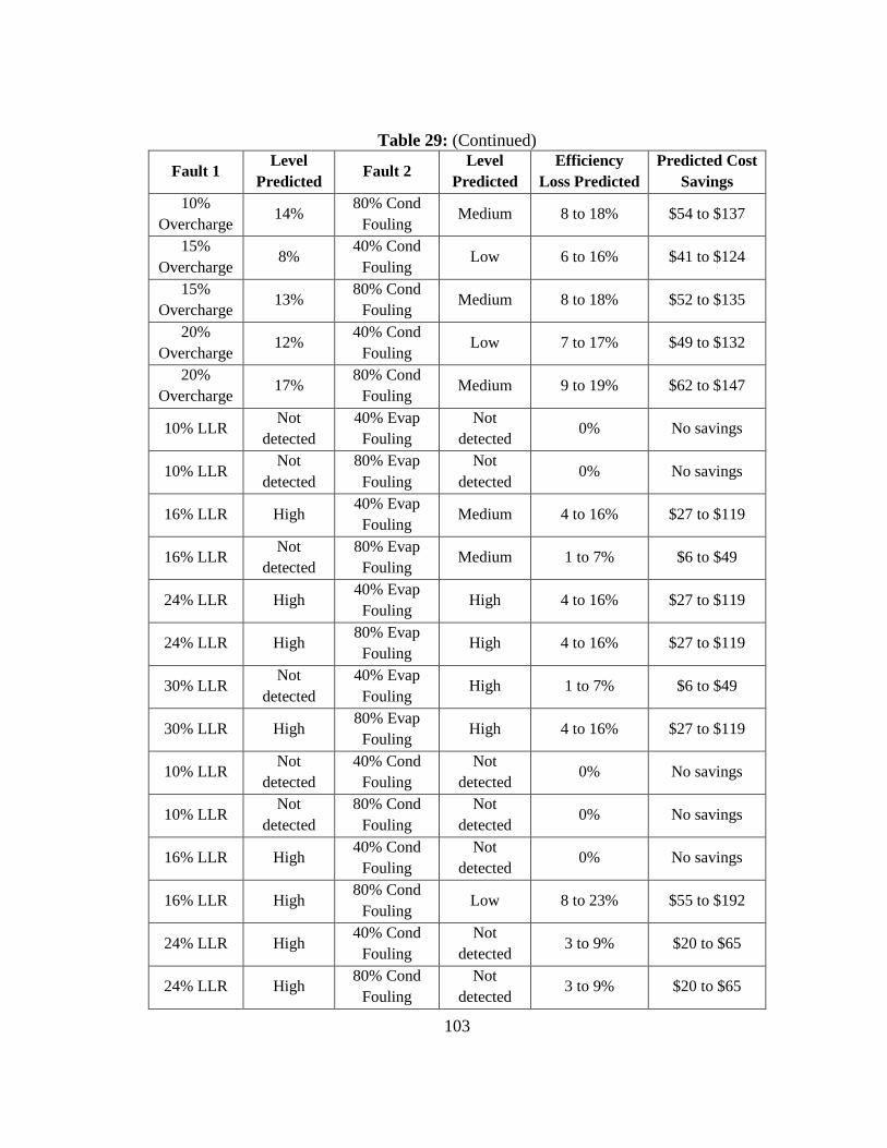
103
Table 29: (Continued)
Fault 1 Level
Predicted Fault 2
Level
Predicted
Efficiency
Loss Predicted
Predicted Cost
Savings
10%
Overcharge 14%
80% Cond
Fouling Medium 8 to 18% $54 to $137
15%
Overcharge 8%
40% Cond
Fouling Low 6 to 16% $41 to $124
15%
Overcharge 13%
80% Cond
Fouling Medium 8 to 18% $52 to $135
20%
Overcharge 12%
40% Cond
Fouling Low 7 to 17% $49 to $132
20%
Overcharge 17%
80% Cond
Fouling Medium 9 to 19% $62 to $147
10% LLR Not
detected
40% Evap
Fouling
Not
detected 0% No savings
10% LLR Not
detected
80% Evap
Fouling
Not
detected 0% No savings
16% LLR High 40% Evap
Fouling Medium 4 to 16% $27 to $119
16% LLR Not
detected
80% Evap
Fouling Medium 1 to 7% $6 to $49
24% LLR High 40% Evap
Fouling High 4 to 16% $27 to $119
24% LLR High 80% Evap
Fouling High 4 to 16% $27 to $119
30% LLR Not
detected
40% Evap
Fouling High 1 to 7% $6 to $49
30% LLR High 80% Evap
Fouling High 4 to 16% $27 to $119
10% LLR Not
detected
40% Cond
Fouling
Not
detected 0% No savings
10% LLR Not
detected
80% Cond
Fouling
Not
detected 0% No savings
16% LLR High 40% Cond
Fouling
Not
detected 0% No savings
16% LLR High 80% Cond
Fouling Low 8 to 23% $55 to $192
24% LLR High 40% Cond
Fouling
Not
detected 3 to 9% $20 to $65
24% LLR High 80% Cond
Fouling
Not
detected 3 to 9% $20 to $65

104
Table 29: (Continued)
Fault 1
Level
Predicte
d
Fault 2 Level
Predicted
Efficiency
Loss
Predicted
Predicted
Cost Savings
30% LLR Not
detected
40% Cond
Fouling Not detected Wrong EF Incorrect
30% LLR High 80% Cond
Fouling Not detected 3 to 9% $20 to $65
20% Evap Foul Not
detected 20% Cond Foul Not detected 0% No savings
20% Evap Foul Not
detected 40% Cond Foul Not detected 0% No savings
20% Evap Foul Not
detected 60% Cond Foul Not detected 0% No savings
20% Evap Foul Not
detected 80% Cond Foul Medium 5 to 15% $34 to $115
20% Evap Foul Not
detected
100% Cond
Foul High 5 to 15% $34 to $115
40% Evap Foul Not
detected 20% Cond Foul Not detected 0% No savings
40% Evap Foul Not
detected 40% Cond Foul Not detected 0% No savings
40% Evap Foul Not
detected 60% Cond Foul Not detected 0% No savings
40% Evap Foul Not
detected 80% Cond Foul Medium 5 to 15% $34 to $115
40% Evap Foul Not
detected
100% Cond
Foul High 5 to 15% $34 to $115
60% Evap Foul Not
detected 20% Cond Foul High 5 to 15% $34 to $115
60% Evap Foul Not
detected 40% Cond Foul Not detected 0% No savings
60% Evap Foul Not
detected 60% Cond Foul Not detected 0% No savings
60% Evap Foul Not
detected 80% Cond Foul Medium 5 to 15% $34 to $115
60% Evap Foul Not
detected
100% Cond
Foul High 5 to 15% $34 to $115
80% Evap Foul Not
detected 20% Cond Foul Not detected 0% No savings
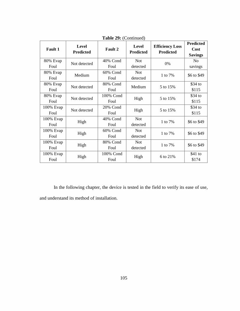
105
Table 29: (Continued)
Fault 1 Level
Predicted Fault 2
Level
Predicted
Efficiency Loss
Predicted
Predicted
Cost
Savings
80% Evap
Foul Not detected
40% Cond
Foul
Not
detected 0%
No
savings
80% Evap
Foul Medium
60% Cond
Foul
Not
detected 1 to 7% $6 to $49
80% Evap
Foul Not detected
80% Cond
Foul Medium 5 to 15%
$34 to
$115
80% Evap
Foul Not detected
100% Cond
Foul High 5 to 15%
$34 to
$115
100% Evap
Foul Not detected
20% Cond
Foul High 5 to 15%
$34 to
$115
100% Evap
Foul High
40% Cond
Foul
Not
detected 1 to 7% $6 to $49
100% Evap
Foul High
60% Cond
Foul
Not
detected 1 to 7% $6 to $49
100% Evap
Foul High
80% Cond
Foul
Not
detected 1 to 7% $6 to $49
100% Evap
Foul High
100% Cond
Foul High 6 to 21%
$41 to
$174
In the following chapter, the device is tested in the field to verify its ease of use,
and understand its method of installation.
106
CHAPTER IX
FIELD TEST
To verify that the device will be quick and easy to install an actual field test was
performed with the proposed device. This chapter goes over how the components of the
proposed device were selected and the process of installation of the device.
Component Selection
The proposed device requires 4 things: temperature sensors, pressure sensors,
data acquisition systems and a laptop with the loaded software. Details about each
component is provided in the following paragraphs:
Temperature Sensors
To keep the measurements non-invasive and make installation of the sensors
quick and easy, the temperature sensors chosen for the proposed device are T-type
thermocouples. The wired T-type thermocouples work well for measurements in
restricted spaces, like the outlet of the compressor that is covered by the condenser fan
and panels. The user may also prefer to measure the evaporator saturated temperature
with a temperature sensor rather than using the pressure measurement to predict the
saturated temperature; in these cases, the T-type thermocouple would work best in the
constricted space of the indoor coil. A clamp type thermocouple would not have allowed
this flexibility.
Therefore, 7 T-type thermocouple wires were used for the proposed device. The
sensors can be mounted using either a thermocouple tape or a temporary paste. The paste

107
is preferred when the thermocouple tape does not stick very well due to condensation on
the tubes.
Pressure Sensors
Pressure measurements are used to estimate the saturated temperatures on the
evaporator and condenser sides. Surface temperature measurements can also be used to
estimate these temperatures, but this would involve guessing the saturation point in the
both coils to decide where to mount the sensor. Therefore, although the pressure
measurements are more expensive and less easy in comparison, they are preferred over
the temperature sensors for a more accurate measurement.
The pressure sensors are installed on the refrigerant charging ports that are found
near the outdoor unit. The pressure sensors chosen for the device had a cable connection
that could be connected to a DC power supply. They gave a 0 to 5 V output, and had a
range of 0 to 300 psig for the evaporator side and 0 to 500 psig for the condenser side.
Mounting the pressure sensor requires a combination fittings and hoses to connect the
pressure sensor to the refrigerant tube. O-rings and Teflon tape are necessary to ensure
that there are no leaks while attaching the sensor.
Data Acquisition Systems
There are 3 DAQs that are needed by the proposed device- one for temperature
measurements on the outdoor unit, one for temperature measurements on the indoor unit
and one for pressure measurements. The DAQ used for measurements on the indoor unit
is a wireless thermocouple DAQ that can communicate to the laptop outside.

108
A multifunction DAQ that can read voltage measurements from the pressure
sensor was used for pressure measurements, and a wired thermocouple DAQ was used
for the remaining temperature measurements at the outdoor unit.
Laptop with Loaded Software
Since the DAQ’s are connected to the laptop, the laptop has to be loaded with
LabVIEW which can be used to record data. NI MAX should also be loaded on the
laptop as it helps troubleshooting the working of the DAQ and checking the connections.
The proposed algorithm of the device was also coded on LabVIEW.
Thus, the chosen set of hardware, is listed in Table 30 and shown in Figure 28.
Table 30: Selected Components used for the Proposed Device
Item
No. Part Description Part Number
Total List
Price
1 USB-6009 Multifunction NI-DAQ 779026-01 $279.00
2 cDAQ-9171, CompactDAQ Chassis (1 slot USB) 781425-01 $259.00
3 cDAQ-9191 CompactDAQ Chassis (1 Slot,
Wireless) 781497-01 $459.00
4 Two NI 9211 4-Channel Thermocouple Input
Module 779001-01 $678.00
5 Power Cord, AC, U.S., 120 VAC, 2.3 meters 763000-01 $9.00
6 Seven T-type Thermocouples (4 to 5 feet long)
$98.00
7 Wired Pressure Transducer Range 0 to 300 psig PX309-300G5V $275.00
8 Wired Pressure Transducer Range 0 to 500 psig PX309-500G5V $275.00
9 Thermocouple Tape
$12.68
10 Teflon Tape
$1.46
11 Flat head screwdriver for NI DAQ 781015-01 $27.90
12 O-rings for Pressure Transducers
$3.37
TOTAL
$2,377.41

109
Figure 28: Components of the Automated Fault Detection and Diagnostic Device
System Description
The system that was tested was a residential, 2 ton split system that used a
Thermal Expansion Valve with R22 refrigerant. The system had a SEER rating of 13,
with constant speed fans and compressor.
Installing the Device
In the field test performed, installing and setting up the device took about 20 minutes
once the different parts of the system were identified. This is provided the following
things are verified before the audit-
The laptop is equipped with LabVIEW and NI MAX.
The wireless DAQ is configured to communicate with the laptop.

110
Knowing where the different components of the air conditioning system are typically
found (condenser, expansion valve, compressor and evaporator) also reduces the time
required to install the device.
Wired DAQ
Multifunction DAQ
DC Power Supply
Figure 29: Data Acquisition Systems Required for the Outdoor Unit

111
Figure 30: Temperature Sensor for Return Air Temperature and the Wireless DAQ at
the Indoor Unit
During the audit, 5 of the 7 temperature sensors were connected to the wired DAQ at
the outdoor unit (Figure 29) and the remaining 2 temperature sensors were connected to
the wireless DAQ indoor (Figure 30). These temperature sensors are mounted as
follows:
One sensor is taped on the low pressure line going towards the condenser, as
close as possible to the evaporator outlet to get a more accurate estimate of
superheat (TERO)(Figure 31).

112
One sensor is taped to the outlet of the condenser (high-pressure line) to get an
estimate of subcooling (TCRO) (Figure 31).
Temperature of Refrigerant at
Condenser Outlet
Temperature of Refrigerant at
Evaporator Outlet
Figure 31: Temperature Sensors for Refrigerant Temperature at Evaporator Outlet and
Condenser Outlet
One sensor is placed right after the compressor. Installing this sensor may require
displacing the condenser fan (TCRI)(Figure 32).
Two sensors are taped at the inlet and outlet of condenser air at the side and at
the top of the outdoor unit respectively (TCAI and TCAO) (Figure 32).
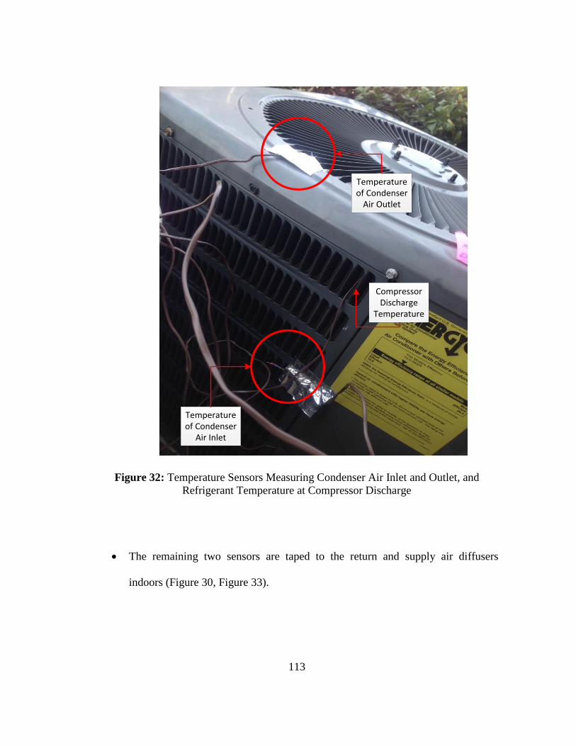
113
Temperature of Condenser
Air Outlet
Temperature of Condenser
Air Inlet
Compressor Discharge
Temperature
Figure 32: Temperature Sensors Measuring Condenser Air Inlet and Outlet, and
Refrigerant Temperature at Compressor Discharge
The remaining two sensors are taped to the return and supply air diffusers
indoors (Figure 30, Figure 33).

114
Temperature of Evaporator
Air Outlet
Figure 33: Temperature Sensor to Measure Supply Air Temperature
The pressure sensors are connected to a hose, which is then connected to the
refrigerant charging port outdoors. The pressure sensors output a voltage value, which is
recorded by the multi-function DAQ and then interpreted by LabVIEW. Installing the
fittings to the refrigerant lines requires Teflon tapes and O-rings to ensure that there are
no leaks while taking measurements. The O-rings are inserted into the thumb screw
valve which fits over the end of the hose that is connect to the refrigerant charging port
(Figure 34).

115
Pressure Sensor
Evaporator Side Pressure Measurement
Figure 34: Mounting of the Pressure Sensor for Evaporator Pressure Measurement
Once the sensors are mounted, the air conditioning unit is turned on and the
LabVIEW code is allowed to run for about 30 minutes. This operation doesn’t need to be
monitored, so while measurements are being recorded, energy auditors are free to look at
other industrial equipment. At the end of 30 minutes, the data is saved, so that the saved
file can be opened with the proposed Fault Detection and Diagnosis algorithm. Basic
user information like SEER rating, type of refrigerant and capacity of the system can be

116
found on the nameplate. Rated SC and SH is found in the installation brochure and the
avoided cost of electricity and operational hours can be estimated.
The few issues that were encountered while installing the sensors in the field test
were-
Sweating on the evaporator outlet line which made it difficult to mount the
sensor. A thermal paste can be used instead to mount the sensors.
Pressure sensors require a DC power source, and if there is no power outlet close
to the outdoor unit this can be an issue. Portable batteries can however be used.
Installing the compressor discharge temperature sensor is time consuming since
it requires removing the condenser fan and placing it back.
The findings of the field test is summarized in Table 31. Overall, the proposed device
was quick and easy to install. In the field test performed, installing and setting up the
device took about 20 minutes, and the data was recorded for about 30 minutes. Based on
the recorded measurements, all the values were within thresholds, and it was confirmed
that the system had no fault.

117
Table 31: Summary of Results from Field Tests
Ease of Installation:
Temperature Sensors Easy and quick.
TCRI sensor may require more time.
Pressure Sensors
Not as easy as the temperature measurements.
Requires multiple fittings, and a power source.
Leaks must be prevented while installing the
sensor.
DAQ The wireless DAQ must be configured to
communicate with the laptop.
Availability of User Information:
Maintenance Brochure SC, SH
Nameplate Refrigerant type, Capacity, SEER rating
Time Required:
Time taken for Installation About 20 minutes
Time taken to collect data About 30 minutes
Time taken for uninstallation About 10 minutes
Results:
Detected Fault None.
Predicted Loss in Efficiency None
Predict Cost Savings None

118
CHAPTER X
CONCLUSION
Based on the results from laboratory tests and field tests it can be said that the
developed device could detect faults and conservatively predict the related efficiency
loss. It can do this with information that is easily available to the technicians performing
an energy audit, and without the need for extensive measurements and tests to develop a
model that is typically needed for fault detection.
All the components of the device cost less than $2,500, which made it affordable.
However, the low cost and mobility of the device is a trade-off for its sensitivity to
faults. The device works well for refrigerant line faults, but detects evaporator and
condenser fouling only at higher levels. This is acceptable, since unlike refrigerant line
faults, the fouling faults are easily visible to energy auditors. In case of multiple fault
tests, it fails to detect both faults in about 40% of the tests, which generally happens for
fault combinations that have opposite effect on the certain feature. However, it predicts
the presence of at least one of the two faults in the remaining 60% of the tests, thus
remaining conservative overall in its energy and cost savings estimate.
Although the rules used by the device were generic so that it could be used for
different types of air conditioners, the sensitivity of the device could be further improved
by using a broader set of thresholds. Thresholds of the features of a system are
dependent on the type of system, its expansion device, its capacity and its SEER rating.

119
Therefore, in the future, a database of thresholds should be developed, and in addition,
further testing could be done on packaged rooftop units, and systems having more than
two simultaneous faults.

120
REFERENCES
[1] U. S. Energy Information Administration, " Annual Energy Review ", 2011.
[2] U. S. Energy Information Administration, "Manufacturing Energy Consumption
Survey ", 2010.
[3] U. S. Energy Information Administration, "International Energy Outlook 2013",
July 2013.
[4] J. L. Pellegrino, N. Margolis, M. Justiniano, M. Miller, and A. Thedki, "Energy
Use, Loss and Opportunities Analysis: U.S. Manufacturing & Mining", prepared
by Energetics, Incorporated and E3M, Incorporated For the U.S. Department of
Energy Energy Efficiency and Renewable Energy Industrial Technologies
Program, December 2004.
[5] A. Zhou, V. Tutterow, J. Harris, and P. Bostrom, "Promoting Energy-Efficient
Buildings in the Industrial Sector ", prepared by Alliance to Save Energy, 2009.
[6] H. Li and J. E. Braun, "Application of Automated Fault Detection and
Diagnostics For Rooftop Air Conditioners in California", presented at the
ACEEE Summer Study on Energy Efficiency in Buildings, Monterey, CA, 2004.
[7] D. E. Stouppe and L. Y.S., "Air Conditioning and Refrigeration Equipment
Failures", National Engineer 93(9), pp. 14-17, 1989.
[8] M. S. Breuker and J. E. Braun, "Common Faults and Their Impacts for Rooftop
Air Conditioners", HVAC&R Research, vol. 4, pp. 303-318, July1998.

121
[9] California Utilities Statewide Codes and Standards Team, "Residential
Refrigerant Charge Testing and Related Issues", for the California Public
Utilties Commission, 2011.
[10] M. Farzad; and D. L. O'Neal., "The Effect of Improper Refrigerant Charging on
the Performance of a Residential Heat Pump with Fixed Expansion Devices
(Capillary Tube and Short Tube Orifice)", 29th Intersociety Energy Conversion
Engineering Conference, pp. 92 I - 926, 1994.
[11] W. Kim and J. E. Braun, "Impacts of Refrigerant Charge on Air Conditioner and
Heat Pump Performance", International Refrigeration and Air Conditioning
Conference, Paper 1122 , 2010.
[12] C. Neme, J. Proctor, and S. Nadel, "Energy Savings Potential from Addressing
Residential Air Conditioner and Heat Pump Installation Problems", prepared for
the American Council for an Energy-Efficient Economy (ACEEE), 1999.
[13] T. Downey and J. Proctor, "What Can 13,000 Air Conditioners Tell Us?", in
American Council for an Energy-Efficient Economy (ACEEE) Conference,
2002.
[14] J. Tomczyk, Troubleshooting An Undercharge of Refrigerant, (2010). Available:
http://www.achrnews.com/articles/troubleshooting-an-undercharge-of-refrigerant
[15] J. Tomczyk, The Professor: Checking on Refrigerant Overcharge, (2010).
Available: http://www.achrnews.com/articles/the-professor-checking-on-
refrigerant-overcharge

122
[16] J. Tomczyk., Diagnosing A Restricted Liquid Line Can Be Tricky, (2002).
Available: http://www.achrnews.com/articles/diagnosing-a-restricted-liquid-line-
can-be-tricky
[17] L. Yang, J. E. Braun, and E. A. Groll, "The Impact of Evaporator Fouling on the
Performance of Packaged Air Conditioners ", presented at the International
Refrigeration and Air Conditioning Conference, Paper 687 , 2004.
[18] R. Isermann, "Process Fault Detection Based on Modeling and Estimation—A
Survey", Automatica, vol. 20, pp. 387, 1984.
[19] M. G. McKellar and D. R. Tree, "Steady State Characteristics of Failures of a
Household Refrigerator " , International Refrigeration and Air Conditioning
Conference. Paper 78, 1988.
[20] L. A. Stallard, "Model Based Expert System for Failure Detection and
Identification of Household Refrigerators", Master’s thesis , Mechanical
Engineering, Purdue University, 1989.
[21] J. Braun and H. Li, "Automated Fault Detection And Diagnostics Of Rooftop Air
Conditioners For California ", prepared for the Architectural Energy Corporation,
August 2003.
[22] H. T. Grimmelius, J. Klein Woud, and G. Been, "On-line Failure Diagnosis for
Compression Refrigeration Plants", International Journal of Refrigeration, vol.
18, pp. 31-41, 1995.

123
[23] M. Stylianou and D. Nikanpour, "Performance Monitoring, Fault Detection, and
Diagnosis of Reciprocating Chillers ", ASHRAE Transactions, vol. 102, pp. 615-
627, 1996.
[24] Y. Jia and T. A. Reddy, "Characteristic Physical Parameter Approach to
Modeling Chillers Suitable for Fault Detection, Diagnosis, and Evaluation",
Journal of Solar Energy Engineering, vol. 125, pp. 258-265, 2003.
[25] M. Yoshimura and N. Ito, "Effective Diagnosis Methods for Air-Conditioning
Equipment in Telecommunications Buildings," in Telecommunications Energy
Conference Proceedin., Eleventh International, Vol 2, pp. 21.1/1-21.1/7, 1989.
[26] T. M. Rossi and J. E. Braun, "A Statistical, Rule-Based Fault Detection and
Diagnostic Method for Vapor Compression Air Conditioners", HVAC&R
Research, vol. 3, pp. 19-37, 1997.
[27] B. Chen and J. E. Braun, "Simple Fault Detection and Diagnosis Methods for
Packaged Air Conditioners", in International Refrigeration and Air
Conditioning Conference, Paper 498, 2000.
[28] H. Li and J. E. Braun, "Decoupling Features and Virtual Sensors for Diagnosis of
Faults in Vapor Compression Air Conditioners", International Journal of
Refrigeration, vol. 30, pp. 546-564, 2007.
[29] P. R. Armstrong, C. R. Laughman, S. B. Leeb, and L. K. Norford, "Detection of
Rooftop Cooling Unit Faults Based on Electrical Measurements", HVAC&R
Research, vol. 12, pp. 151-175, 2006.

124
[30] S. Katipamula and M. R. Brambley, "Review Article: Methods for Fault
Detection, Diagnostics, and Prognostics for Building Systems—A Review, Part
I", HVAC&R Research, vol. 11, pp. 3-25, 2005.
[31] Virtjoule, (2014), Available: http://www.virtjoule.com/
[32] Pacific Northwest National Laboratory, Smart Monitoring and Diagnostic
System, (2013). Available: http://buildingsystems.pnnl.gov/building/smds.stm
[33] Sensus MI, Automatic Early Detection of Machine Faults Diagnosis Indicating
the Cause of the Fault (2014). Available:
http://sensusmi.com/en/index.php?option=com_content&task=view&id=5&Itemi
d=62
[34] ClimaCheck, ClimaCheck Solutions (2014). Available:
http://www.climacheck.com/?p=2
[35] H. Li and J. E. Braun, "Development, Evaluation, and Demonstration of a Virtual
Refrigerant Charge Sensor", HVAC&R Research, vol. 15, pp. 117-136, 2009.
[36] J. B. Watt, "Development Of Empirical Temperature And Humidity-Based
Degraded-Condition Indicators For Low-Tonnage Air Conditioners", Master's
thesis, Mechanical Engineering, Texas A&M University, 1997.


