Designing Parking Facilities for Autonomous Vehicles
Mehdi Nourinejad*a, Sina Bahramib, Matthew J. Roordac
aDepartment of Civil Engineering, University of Toronto, Toronto, [email protected]
bDepartment of Civil Engineering, University of Toronto, Toronto, [email protected]
cDepartment of Civil Engineering, University of Toronto, Toronto, [email protected]
Abstract
Autonomous vehicles will have a major impact on car-park designs in the future. While
existing parking facilities have islands with only two rows of vehicles, future designs tailored
for autonomous vehicles can have multiple rows of vehicles stacked behind each other which
can cause blockage of some vehicles. Nevertheless, the driverless feature of autonomous
vehicles allows car-park operators to relocate vehicles and create a clear pathway for blocked
cars to leave the facility. This paper investigates the problem of finding the optimal car-
park layout design that minimizes relocations while fitting a given number of vehicles in
the car-park. To solve the layout design problem, we present a mixed-integer non-linear
program that treats each island in the facility as a queuing system and solve it using Benders
decomposition for an exact answer. We also present a heuristic model to find a reasonable
upper-bound of the mathematical model. We show that autonomous vehicle car-parks can
decrease the need for parking space by an average of 60% and a maximum of 90%. This
substantial revitalization of space that was previously used for parking can lead to more
socially beneficial purposes when car-parks are converted into commercial and residential
land-uses.
Keywords: Autonomous vehicle; Parking; Facility layout; Benders decomposition;
Queuing systems
1. Introduction
Parking is an important part of transportation planning as a typical vehicle spends 95
percent of its lifetime sitting in a parking spot (Mitchell, 2015). The increasing need to store
vehicles has transformed a lot of valuable real-estate into parking garages in many countries.
In the United States approximately 6,500 square miles of land is devoted to parking which is
larger than the entire state of Connecticut (Chester et al., 2011; Thompson, 2016). Allocating
Preprint submitted to Elsevier June 29, 2017
valuable land to parking subsequently increases renting costs and parking acquisition costs
in major downtown cores. One example is Hong Kong where the average cost of one parking
space is as high as 180 thousand USD (South China Morning Post, 2015). Realizing the high
social cost of parking provision, Autonomous Vehicle (AV) industry leaders are rethinking
how to reduce the parking footprint by converting traditional parking lots into automated
parking facilities that can store more AVs (compared to regular vehicles) in smaller areas.
In this study, we investigate the optimal design and management of such facilities.
AVs can reduce the parking footprint in several ways. As vehicles become driver-less,
the passengers no longer need to be physically present in car-parks. Driver-less AVs drop
off their passengers at the parking entrance (or at a designated drop-off zone) and head to a
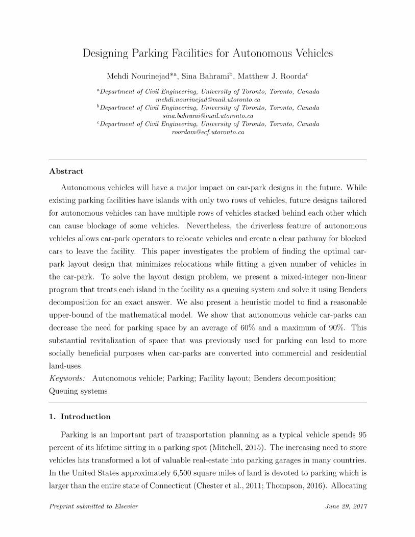
spot chosen by the car-park operator. In this automated parking system, the average space
per vehicle is estimated to be reduced by 2 square meters per vehicle as the driving lanes
become narrower, elevators and staircases become obsolete, and as the required room for
opening a vehicle’s doors becomes discarded (see Fig. 1) (TechWorld , 2016).
Motivated by the benefits of AV parking and its impact on revitalizing valuable real-
estate, auto makers are collaborating with cities to create the first generation of AV parking
facilities. Audi’s Urban Futures Initiative is among the programs that is implementing a pilot
to measure the impact of AV parking on land restoration. The pilot is estimated to save up
to 62% in parking space by 2030 which is equivalent to $100 million USD in the district of
Assembly Row which is the focus of the project (DesignBoom, 2015). Tesla, another leader
in AV technology, is also improving parking by offering an auto-pilot system called “Smart
Summon” which allows the vehicle to navigate complex environments and parking spaces
whenever summoned by its owner. Such auto-parking systems in AVs will pave the way for
the next generation of AV parking facilities with improved space efficiency.
One additional way to increase car-park space efficiency (in addition to removal of ele-
vators, etc.) is to stack the AVs in several rows, one behind the other as shown in Fig. 1b.
While this type of layout reduces parking space, it can cause blockage if a certain vehicle
is barricaded by other vehicles and cannot leave the facility. To release barricaded vehicles,
the car-park operator has to relocate some of the vehicles around to create a clear pathway
for the blocked vehicle to exit. The extent of vehicle relocation depends on the layout of
car-park (i.e., number of rows) which should ideally be desgined so that prking occupancy
(i.e., number of vehicles in the car-park) is high and vehicle relocation is low.
The optimal layout of the car-park has a great impact on space efficiency. Existing
layouts divide the facility into a number of islands and roadways. The islands are used
2
to store vehicles while the roadways separate the islands and allow vehicles to maneuver
when searching for a desirable spot. To ensure that no vehicle gets blocked, the islands
hold no more than two rows of vehicles in conventional car-park designs (see Fig. 1a) which
consequently leads to waste of space. With AV technology, however, the islands can have
more than two rows and the roadways can be narrower. An eminent research question that
arise is: How should we design AV parking facilities that store a large number of AVs with
minimal relocations? To answer this question, we pursue the following objectives throughout
this study:
• We present a model to find the optimal layout of a parking facility for AVs.
• We define a relocation strategy that ensures a smooth retrieval of any AV that is
summoned by its user.
• We present exact and heuristic algorithms to find the optimal AV car-park layout.
• We find the maximum number of AVs that can be fit in car-park with given dimensions.
• We quantify the required parking space reduction when the car-park is exclusively
designed for a given demand of AVs.
The remainder of this paper is organized as follows: We present a background on AV
models in Section 2, a model to find the optimal car-park layout in Section 3, two solutions
algorithms in Section 4, numerical experiments in Section 5, and the conclusions of the study
in Section 6.
2. Background
With the rapid advancement in AV technologies, AVs are expected to enter the consumer
market in the next decade (Fagnant and Kockelman, 2015). Already, AV technology leaders
such as Google’s Waymo have tested AVs over than 3 million miles in several U.S. cities
(Waymo, 2016). While full implementation of AVs is hindered by many practical challenges,
recent studies are looking at ways of addressing these challenges and finding novel ways of
exploiting the full potential of AVs. The current AV studies focus on traffic flow (Levin
and Boyles, 2016; de Almeida Correia and van Arem, 2016; Mahmassani, 2016; Talebpour
and Mahmassani, 2016; de Oliveira, 2017), safety (Katrakazas et al., 2015; Kalra and Pad-
dock, 2016), intersection control (Le Vine et al., 2015; Yang and Monterola, 2016), emissions
3
Street Access
STR
EET
DR
IVE
WA
Y
Building
Street Access
STR
EET
DR
IVE
WA
Y
Building
(a) (b)
Figure 1: (a) Conventional parking design, (b) parking design for autonomous vehicles.
(Greenblatt and Saxena, 2015; Mersky and Samaras, 2016), and sharing AVs between mul-
tiple users (Fagnant and Kockelman, 2014; Chen et al., 2016a,b; Krueger et al., 2016). AVs
will also significantly change parking behavior by allowing the vehicles to self-park, a trait
that the general public is very enthusiatic about. In a recent survey of 5,600 people in 10
countries conducted by the World Economic Forum, 43.5% of the respondents reported that
the biggest benefit of AV technology is its self-parking capability (Mitchell, 2015).
Parking behavior is argued to be influenced by AVs in several ways. Given that they can
self-park, AVs no longer need to be in close proximity of their drivers. Instead, they can be
dispatched to less congested parking lots that are farther away and cheaper (Fagnant and
Kockelman, 2015). This implies that human drivers can get dropped off right at their final
destination without having to search for a spot or having to walk from that spot to their
final destination. Nourinejad and Roorda (2017) model this parking behavior and show city
planners can allocate parking to AVs at locations that are farther away from downtown.
From a technological standpoint, the design and management of car-parks will need
to change. Car-parks for regular vehicles are commonly designed according to guidelines
published by local governments. The City of Toronto, for example, imposes restrictions on
parking space dimensions, orientation of spaces, and the width of the driving aisles (City of
Toronto, 2013). Current guidelines are not readily applicable to AVs because they do not
consider the possible AV movements within the car-park. Hence, there is a need to initiate
a new set of regulations tailored for AV parking.
Although there are currently no guidelines for AV parking design, there are several re-
4
search streams that exhibit similar properties to the problem at hand. We specify these
streams as the following:
• The stacking problem: Many storage systems require that items (i.e., any type of mer-
chandise) be stacked on top of each other to increase space efficiency (De Castilho and
Daganzo, 1993; Zhang et al., 2002; Jiang and Jin, 2017). In these systems, retrieving
a blocked item (i.e., an item that is not on top of the stack) requires some rehandling.
Storage operators ideally like to minimize rehandling by optimally stacking items. A
similar objective is pursued in AV parking design. We like to fit the AVs in the car-park
to minimize the number of relocations whenever retrieving a blocked vehicle.
• Parking assignment : Finding a parking space in downtown cores is often time-consuming
and difficult. In a survey of 20 cities around the world, it was reported that drivers
spend 20 minutes on average to find parking (Gallivan, 2011). To address this issue,
several studies have focused on modeling search behavior (Boyles et al., 2015; Liu and
Geroliminis, 2016; Pel and Chaniotakis, 2017) or developing models that assign park-
ing spaces to vehicles in an optimal fashion (He et al., 2015; Shao et al., 2016; Lei and
Ouyang, 2017). Parking assignment also appears in the AV parking design problem.
The challenge is to assign the vehicles to the islands of the facility in a balanced way.
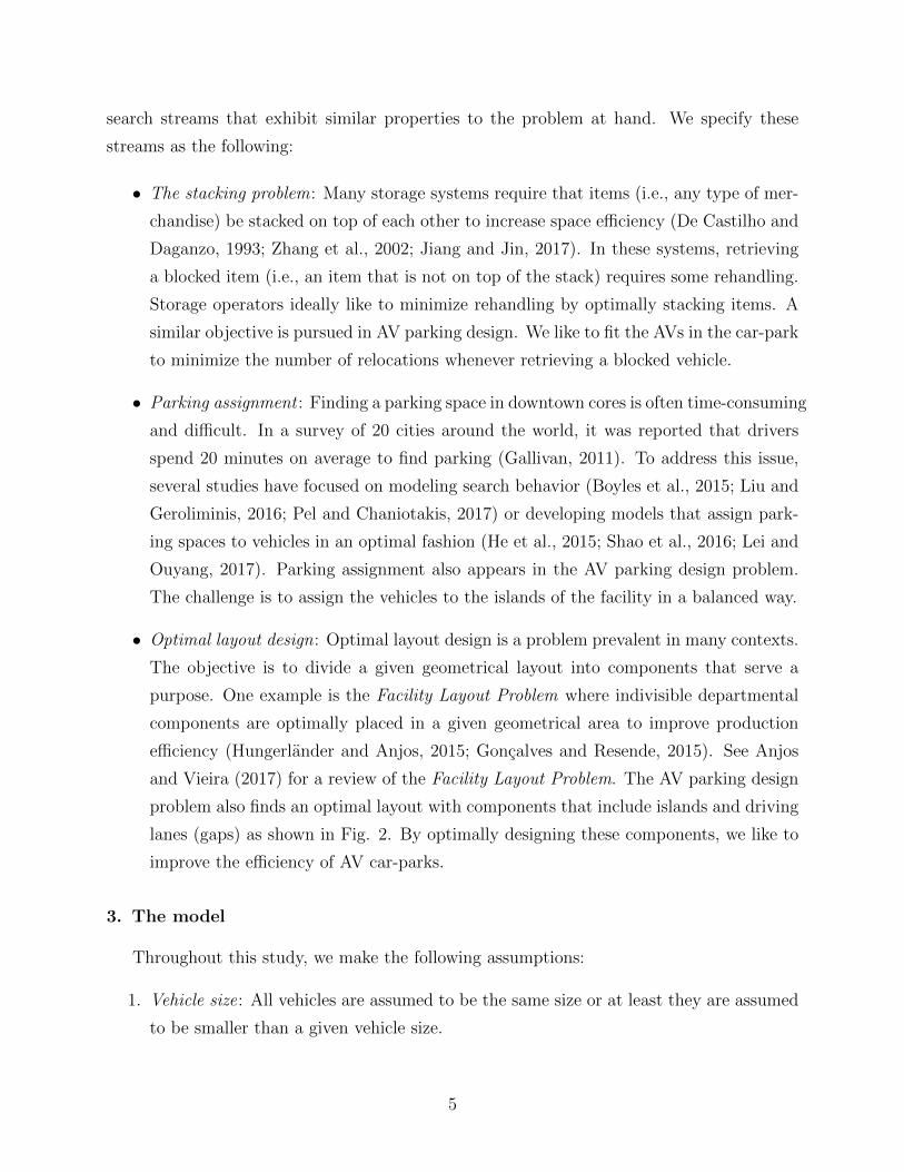
• Optimal layout design: Optimal layout design is a problem prevalent in many contexts.
The objective is to divide a given geometrical layout into components that serve a
purpose. One example is the Facility Layout Problem where indivisible departmental
components are optimally placed in a given geometrical area to improve production
efficiency (Hungerlander and Anjos, 2015; Goncalves and Resende, 2015). See Anjos
and Vieira (2017) for a review of the Facility Layout Problem. The AV parking design
problem also finds an optimal layout with components that include islands and driving
lanes (gaps) as shown in Fig. 2. By optimally designing these components, we like to
improve the efficiency of AV car-parks.
3. The model
Throughout this study, we make the following assumptions:
1. Vehicle size: All vehicles are assumed to be the same size or at least they are assumed
to be smaller than a given vehicle size.
5
2. Vehicle control : We assume that the facility operator takes control of all AVs that
enter the parking facility. The operator can then relocate the vehicles within the
facility whenever required. When a vehicle leaves the facility, the control of the AV is
directed back to the vehicle owner.
3. Vehicle arrival : The vehicles arrive at the parking facility in a Poisson manner with
arrival rate λ [vehicles/hour] and their parking duration (i.e., parking time) follows an
exponential distribution with an average parking time of µ [hours].
4. Exclusively for autonomous vehicles : We assume that the parking facility is exclusively
designed for AVs.
The nomenclature of the model is as follows.
Nomenclature
Parameters
D Design demand [vehicles ]
λ Arrival rate of vehicles [vehicles per hour ]
µ Average parking time [hours ]
L Length of the land plot
W Width of the land plot
l Length of each parking spot
w Width of each parking spot
y Number of vehicle rows in each island
α Width of each driving lane in the inter-island gaps
S Maximum possible number of islands in the facility
K Maximum number of spots in each stack of the facility
Sets
I Set of islands
Decision variables
xi Half the number of columns in island i
ei Inter-island gap between island i and i+ 1 allocated to vehicle movements
gi Inter-island gap between island i and i+ 1 allocated to temporary vehicle storage
di Demand allocated to island i
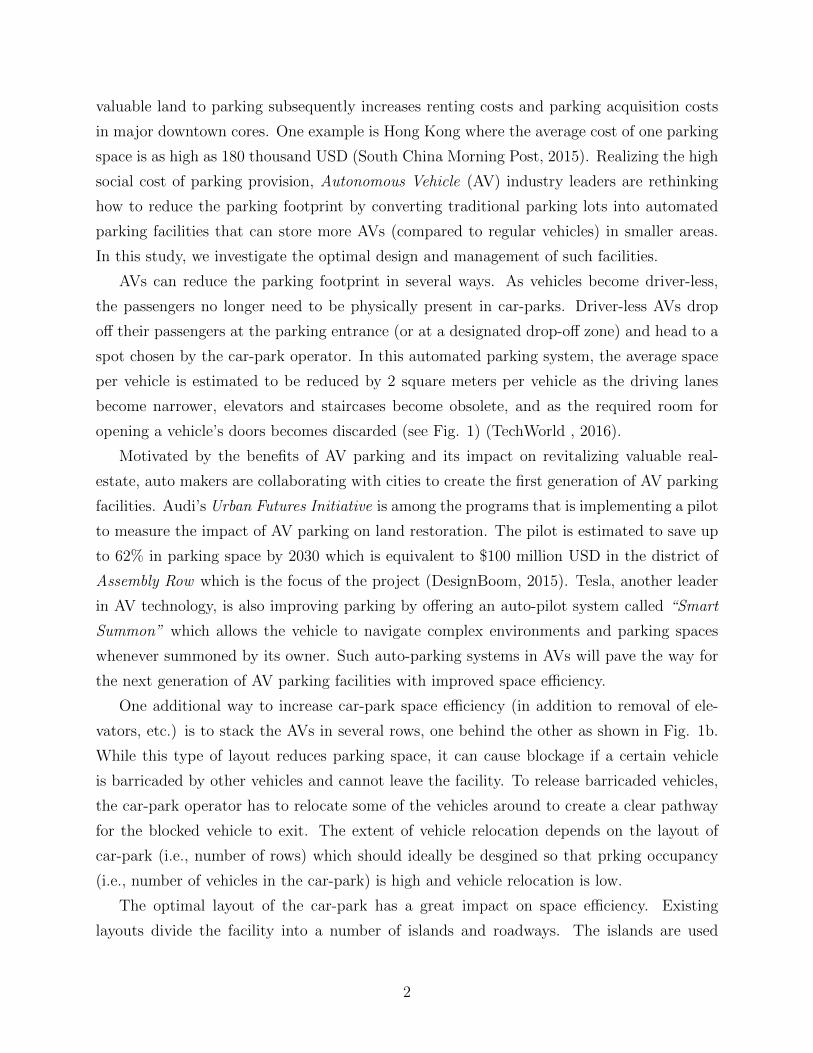
3.1. Geometric properties of the facility
Consider a rectangular plot of land with length L and width W that has to be converted
into an AV parking facility. Assume that the parking facility has a number of islands (See
6
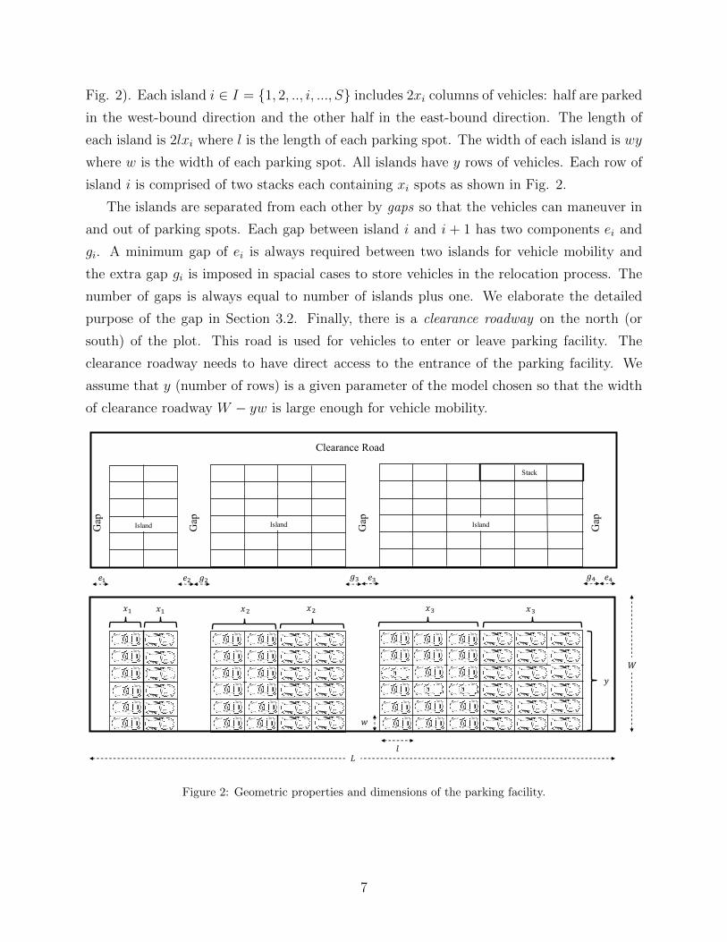
Fig. 2). Each island i ∈ I = {1, 2, .., i, ..., S} includes 2xi columns of vehicles: half are parked
in the west-bound direction and the other half in the east-bound direction. The length of
each island is 2lxi where l is the length of each parking spot. The width of each island is wy
where w is the width of each parking spot. All islands have y rows of vehicles. Each row of
island i is comprised of two stacks each containing xi spots as shown in Fig. 2.
The islands are separated from each other by gaps so that the vehicles can maneuver in
and out of parking spots. Each gap between island i and i + 1 has two components ei and
gi. A minimum gap of ei is always required between two islands for vehicle mobility and
the extra gap gi is imposed in spacial cases to store vehicles in the relocation process. The
number of gaps is always equal to number of islands plus one. We elaborate the detailed
purpose of the gap in Section 3.2. Finally, there is a clearance roadway on the north (or
south) of the plot. This road is used for vehicles to enter or leave parking facility. The
clearance roadway needs to have direct access to the entrance of the parking facility. We
assume that y (number of rows) is a given parameter of the model chosen so that the width
of clearance roadway W − yw is large enough for vehicle mobility.
𝑥" 𝑥" 𝑥# 𝑥# 𝑥$ 𝑥$
𝑒#𝑒" 𝑔$ 𝑒$ 𝑔' 𝑒'
𝑤
𝑙
𝑦
𝑔#
𝐿
𝑊
Clearance Road
Gap
Gap
Gap
GapIsland Island Island
Stack
Figure 2: Geometric properties and dimensions of the parking facility.
7
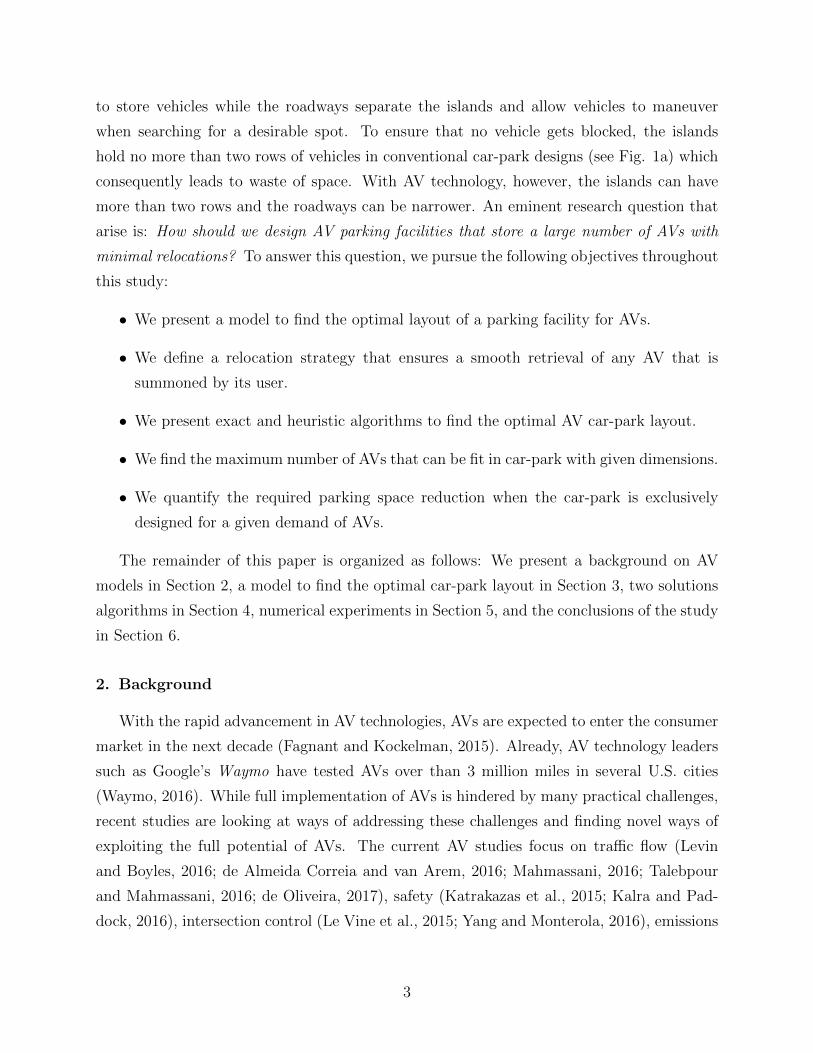
3.2. Relocation strategy
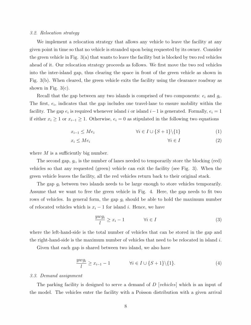
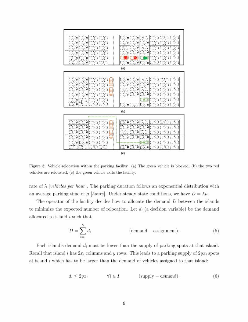
We implement a relocation strategy that allows any vehicle to leave the facility at any
given point in time so that no vehicle is stranded upon being requested by its owner. Consider
the green vehicle in Fig. 3(a) that wants to leave the facility but is blocked by two red vehicles
ahead of it. Our relocation strategy proceeds as follows. We first move the two red vehicles
into the inter-island gap, thus clearing the space in front of the green vehicle as shown in
Fig. 3(b). When cleared, the green vehicle exits the facility using the clearance roadway as
shown in Fig. 3(c).
Recall that the gap between any two islands is comprised of two components: ei and gi.
The first, ei, indicates that the gap includes one travel-lane to ensure mobility within the
facility. The gap ei is required whenever island i or island i−1 is generated. Formally, ei = 1
if either xi ≥ 1 or xi−1 ≥ 1. Otherwise, ei = 0 as stipulated in the following two equations
xi−1 ≤Mei ∀i ∈ I ∪ {S + 1}\{1} (1)
xi ≤Mei ∀i ∈ I (2)
where M is a sufficiently big number.
The second gap, gi, is the number of lanes needed to temporarily store the blocking (red)
vehicles so that any requested (green) vehicle can exit the facility (see Fig. 3). When the
green vehicle leaves the facility, all the red vehicles return back to their original stack.
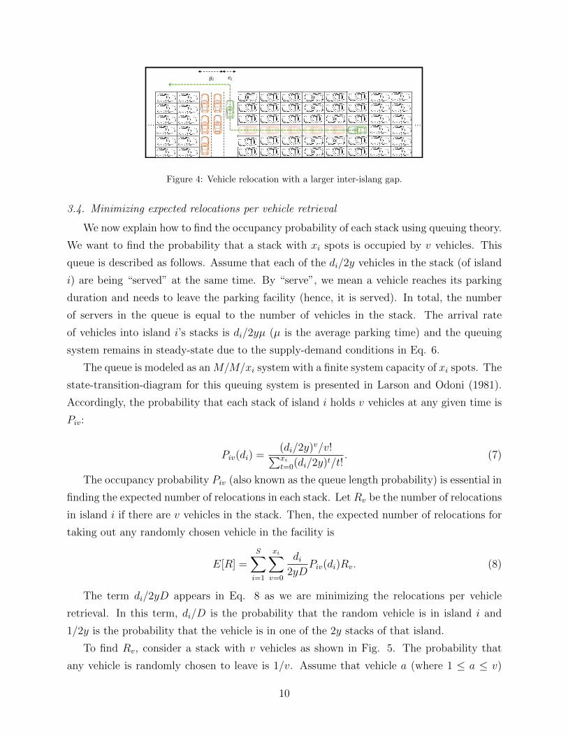
The gap gi between two islands needs to be large enough to store vehicles temporarily.
Assume that we want to free the green vehicle in Fig. 4. Here, the gap needs to fit two
rows of vehicles. In general form, the gap gi should be able to hold the maximum number
of relocated vehicles which is xi − 1 for island i. Hence, we have
ywgil≥ xi − 1 ∀i ∈ I (3)
where the left-hand-side is the total number of vehicles that can be stored in the gap and
the right-hand-side is the maximum number of vehicles that need to be relocated in island i.
Given that each gap is shared between two island, we also have
ywgil≥ xi−1 − 1 ∀i ∈ I ∪ {S + 1}\{1}. (4)
3.3. Demand assignment
The parking facility is designed to serve a demand of D [vehicles ] which is an input of
the model. The vehicles enter the facility with a Poisson distribution with a given arrival
8
(a)
(b)
(c)
……
……
……
Figure 3: Vehicle relocation within the parking facility. (a) The green vehicle is blocked, (b) the two red
vehicles are relocated, (c) the green vehicle exits the facility.
rate of λ [vehicles per hour ]. The parking duration follows an exponential distribution with
an average parking time of µ [hours ]. Under steady state conditions, we have D = λµ.
The operator of the facility decides how to allocate the demand D between the islands
to minimize the expected number of relocation. Let di (a decision variable) be the demand
allocated to island i such that
D =S∑
i=1
di (demand− assignment). (5)
Each island’s demand di must be lower than the supply of parking spots at that island.
Recall that island i has 2xi columns and y rows. This leads to a parking supply of 2yxi spots
at island i which has to be larger than the demand of vehicles assigned to that island:
di ≤ 2yxi ∀i ∈ I (supply − demand). (6)
9
……
𝑒"𝑔"
Figure 4: Vehicle relocation with a larger inter-islang gap.
3.4. Minimizing expected relocations per vehicle retrieval
We now explain how to find the occupancy probability of each stack using queuing theory.
We want to find the probability that a stack with xi spots is occupied by v vehicles. This
queue is described as follows. Assume that each of the di/2y vehicles in the stack (of island
i) are being “served” at the same time. By “serve”, we mean a vehicle reaches its parking
duration and needs to leave the parking facility (hence, it is served). In total, the number
of servers in the queue is equal to the number of vehicles in the stack. The arrival rate
of vehicles into island i’s stacks is di/2yµ (µ is the average parking time) and the queuing
system remains in steady-state due to the supply-demand conditions in Eq. 6.
The queue is modeled as an M/M/xi system with a finite system capacity of xi spots. The
state-transition-diagram for this queuing system is presented in Larson and Odoni (1981).
Accordingly, the probability that each stack of island i holds v vehicles at any given time is
Piv:
Piv(di) =(di/2y)v/v!∑xi
t=0(di/2y)t/t!. (7)
The occupancy probability Piv (also known as the queue length probability) is essential in
finding the expected number of relocations in each stack. Let Rv be the number of relocations
in island i if there are v vehicles in the stack. Then, the expected number of relocations for
taking out any randomly chosen vehicle in the facility is
E[R] =S∑
i=1
xi∑v=0
di2yD
Piv(di)Rv. (8)
The term di/2yD appears in Eq. 8 as we are minimizing the relocations per vehicle
retrieval. In this term, di/D is the probability that the random vehicle is in island i and
1/2y is the probability that the vehicle is in one of the 2y stacks of that island.
To find Rv, consider a stack with v vehicles as shown in Fig. 5. The probability that
any vehicle is randomly chosen to leave is 1/v. Assume that vehicle a (where 1 ≤ a ≤ v)
10
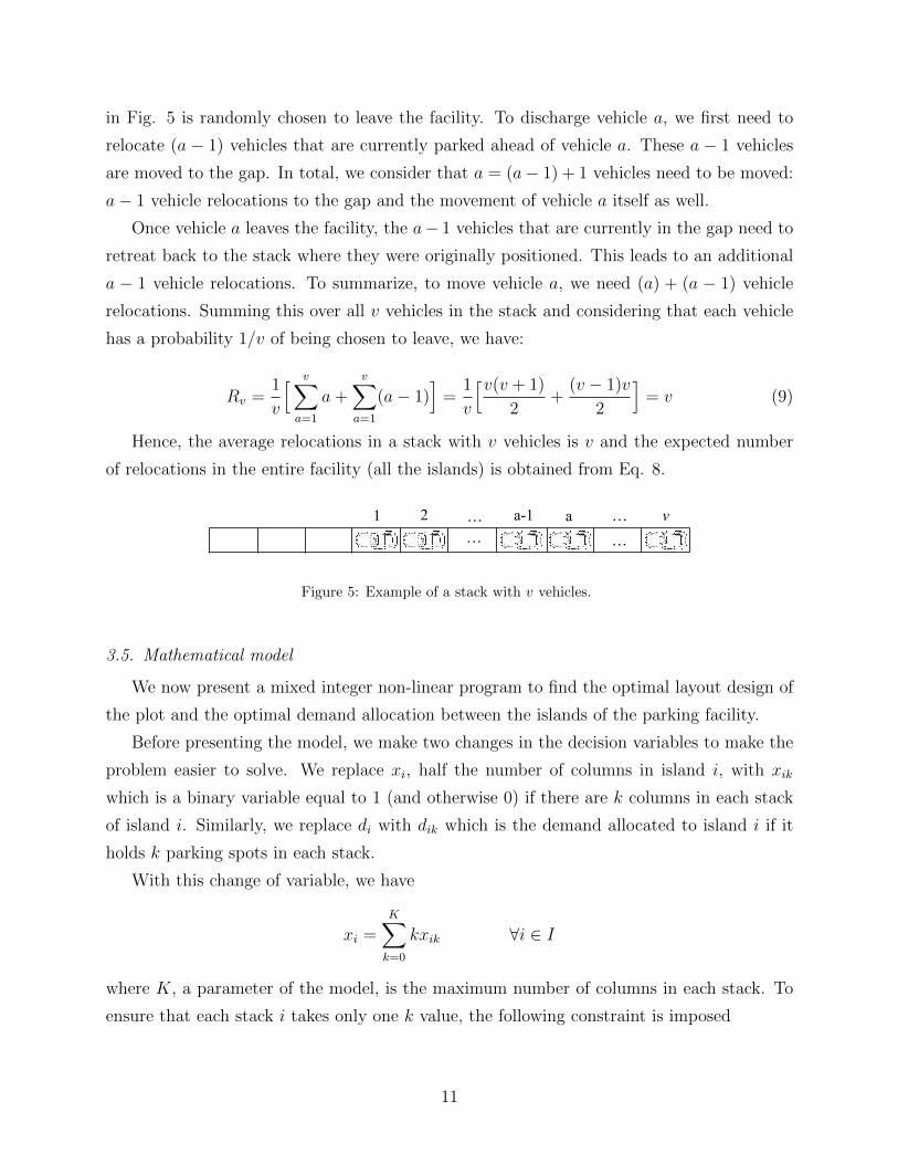
in Fig. 5 is randomly chosen to leave the facility. To discharge vehicle a, we first need to
relocate (a − 1) vehicles that are currently parked ahead of vehicle a. These a − 1 vehicles
are moved to the gap. In total, we consider that a = (a− 1) + 1 vehicles need to be moved:
a− 1 vehicle relocations to the gap and the movement of vehicle a itself as well.
Once vehicle a leaves the facility, the a− 1 vehicles that are currently in the gap need to
retreat back to the stack where they were originally positioned. This leads to an additional
a − 1 vehicle relocations. To summarize, to move vehicle a, we need (a) + (a − 1) vehicle
relocations. Summing this over all v vehicles in the stack and considering that each vehicle
has a probability 1/v of being chosen to leave, we have:
Rv =1
v
[ v∑a=1
a+v∑
a=1
(a− 1)]
=1
v
[v(v + 1)
2+
(v − 1)v
2
]= v (9)
Hence, the average relocations in a stack with v vehicles is v and the expected number
of relocations in the entire facility (all the islands) is obtained from Eq. 8.
…1 a-1 v… …a
…2
Figure 5: Example of a stack with v vehicles.
3.5. Mathematical model
We now present a mixed integer non-linear program to find the optimal layout design of
the plot and the optimal demand allocation between the islands of the parking facility.
Before presenting the model, we make two changes in the decision variables to make the
problem easier to solve. We replace xi, half the number of columns in island i, with xik
which is a binary variable equal to 1 (and otherwise 0) if there are k columns in each stack
of island i. Similarly, we replace di with dik which is the demand allocated to island i if it
holds k parking spots in each stack.
With this change of variable, we have
xi =K∑k=0
kxik ∀i ∈ I
where K, a parameter of the model, is the maximum number of columns in each stack. To
ensure that each stack i takes only one k value, the following constraint is imposed
11
K∑k=0
xik = 1 ∀i ∈ I.
Subsequently, the supply-demand constraint in Eq. 6 changes to
dik ≤ 2y k xik ∀i ∈ I.
The relocation strategy constraints (Eq. 3 and Eq. 4) become, respectively,
ywgil≥
K∑k=0
kxik − 1 ∀i ∈ I
andywgil≥
K∑k=0
kxi−1,k − 1 ∀i ∈ I ∪ {S + 1}\{1}
and the gap constraints (Eq. 1 and Eq. 2) become, respectively,
K∑k=0
kxi−1,k ≤Mei ∀i ∈ I ∪ {S + 1}\{1}
andK∑k=0
kxik ≤Mei ∀i ∈ I.
Using the new definition xik, we also change the queue occupancy probabilities Piv to
the following. Let Pikv be the probability that a stack of island i with capacity k holds v
vehicles. This probability is obtained with minor modification of Eq. 7:
Pikv(dik) =(dik/2y)v/v!∑kt=0(dik/2y)t/t!
.
The mathematical model, denoted as the Layout Design [LD] Problem is formally defined
as
[LD] : Minimize E[R] =S∑
i=1
K∑k=0
k∑v=0
xikPikv(dik)Rv dik/2yD (10)
subject to
D =S∑
i=1
K∑k=0
dik (11)
dik ≤ 2y k xik ∀i ∈ I,∀k (12)
12
K∑k=0
xik = 1 ∀i ∈ I (13)
ywgil≥
K∑k=0
kxik − 1 ∀i ∈ I (14)
ywgil≥
K∑k=0
kxi−1,k − 1 ∀i ∈ I ∪ {S + 1}\{1} (15)
K∑k=0
kxi−1,k ≤Mei ∀i ∈ I ∪ {S + 1}\{1} (16)
K∑k=0
kxik ≤Mei ∀i ∈ I (17)
2lS∑
i=1
K∑k=0
kxik + αS+1∑i=1
(ei + gi) ≤ L (18)
ei ∈ {0, 1} ∀i ∈ I ∪ {S + 1} (19)
gi, xik ∈ Z ∀i ∈ I,∀k (20)
xik, ei, gi, dik ≥ 0 ∀i ∈ I,∀k (21)
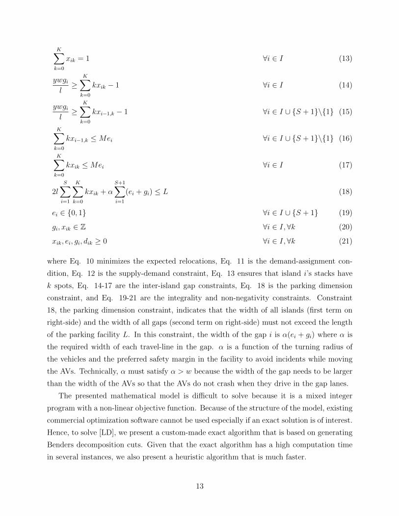
where Eq. 10 minimizes the expected relocations, Eq. 11 is the demand-assignment con-
dition, Eq. 12 is the supply-demand constraint, Eq. 13 ensures that island i’s stacks have
k spots, Eq. 14-17 are the inter-island gap constraints, Eq. 18 is the parking dimension
constraint, and Eq. 19-21 are the integrality and non-negativity constraints. Constraint
18, the parking dimension constraint, indicates that the width of all islands (first term on
right-side) and the width of all gaps (second term on right-side) must not exceed the length
of the parking facility L. In this constraint, the width of the gap i is α(ei + gi) where α is
the required width of each travel-line in the gap. α is a function of the turning radius of
the vehicles and the preferred safety margin in the facility to avoid incidents while moving
the AVs. Technically, α must satisfy α > w because the width of the gap needs to be larger
than the width of the AVs so that the AVs do not crash when they drive in the gap lanes.
The presented mathematical model is difficult to solve because it is a mixed integer
program with a non-linear objective function. Because of the structure of the model, existing
commercial optimization software cannot be used especially if an exact solution is of interest.
Hence, to solve [LD], we present a custom-made exact algorithm that is based on generating
Benders decomposition cuts. Given that the exact algorithm has a high computation time
in several instances, we also present a heuristic algorithm that is much faster.
13
4. Solution methodology
4.1. An exact decomposition algorithm
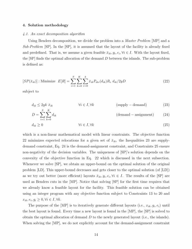
Using Benders decomposition, we divide the problem into a Master Problem [MP] and a
Sub-Problem [SP]. In the [SP], it is assumed that the layout of the facility is already fixed
and predefined. That is, we assume a given feasible xik, gi, ei,∀i ∈ I. With the layout fixed,
the [SP] finds the optimal allocation of the demand D between the islands. The sub-problem
is defined as:
[SP (xik)] : Minimize E[R] =S∑
i=1
K∑k=0
k∑v=0
xikPikv(dik)Rv dik/2yD (22)
subject to
dik ≤ 2yk xik ∀i ∈ I,∀k (supply − demand) (23)
D =S∑
i=1
K∑k=0
dik (demand− assignment) (24)
dik ≥ 0 ∀i ∈ I,∀k (25)
which is a non-linear mathematical model with linear constraints. The objective function
22 minimizes expected relocations for a given set of xik, the Inequalities 23 are supply-
demand constraint, Eq. 24 is the demand-assignment constraint, and Constraints 25 ensure
non-negativity of the decision variables. The uniqueness of [SP]’s solution depends on the
convexity of the objective function in Eq. 22 which is discussed in the next subsection.
Whenever we solve [SP], we obtain an upper-bound on the optimal solution of the original
problem [LD]. This upper-bound decreases and gets closer to the optimal solution (of [LD])
as we try out better (more efficient) layouts xik, gi, ei,∀i ∈ I. The results of the [SP] are
used as Benders cuts in the [MP]. Notice that solving [SP] for the first time requires that
we already know a feasible layout for the facility. This feasible solution can be obtained
using an integer program with any objective function subject to Constraints 13 to 20 and
xik, ei, gi ≥ 0,∀i ∈ I,∀k.
The purpose of the [MP] is to iteratively generate different layouts (i.e., xik, gi, ei) until
the best layout is found. Every time a new layout is found in the [MP], the [SP] is solved to
obtain the optimal allocation of demand D to the newly generated layout (i.e., the islands).
When solving the [MP], we do not explicitly account for the demand-assignment constraint
14
(Eq. 24) as this constraint has already applied in the [SP]. However, the supply-demand
constraints (Inequality 23) is actually implicitly considered in the form of Benders cuts in
the [MP]. The supply-demand constraint is the only constraint that connects facility layout
to demand assignment.
By solving [MP], we find a lower-bound on the optimal objective function of the original
problem [LD] because the [MP] is missing the supply-demand constraints in Eq. 12. Absence
of these constraints indicates that the objective of the [MP] is always better (lower) than the
true objective of [LD]. Hence, the [MP] provides a lower-bound for [LD]. The [SP]’s solution
is accounted in the [MP] using Benders cuts constraints.
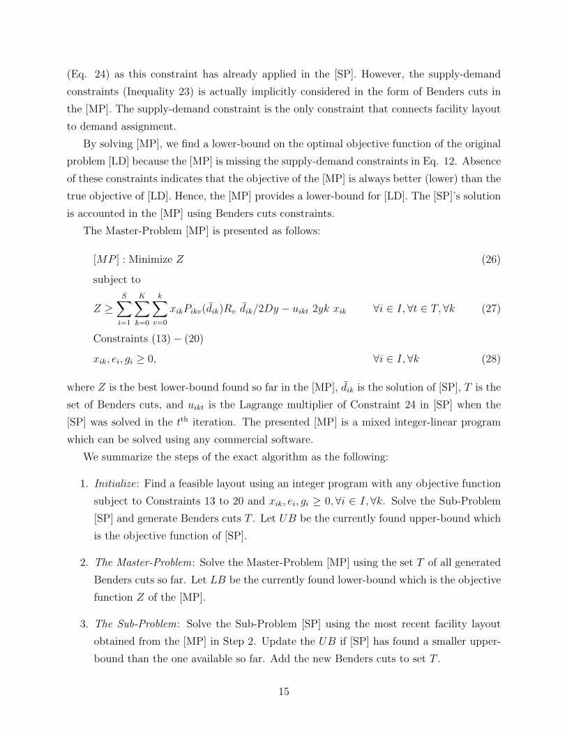
The Master-Problem [MP] is presented as follows:
[MP ] : Minimize Z (26)
subject to
Z ≥S∑
i=1
K∑k=0
k∑v=0
xikPikv(dik)Rv dik/2Dy − uikt 2yk xik ∀i ∈ I,∀t ∈ T,∀k (27)
Constraints (13)− (20)
xik, ei, gi ≥ 0, ∀i ∈ I,∀k (28)
where Z is the best lower-bound found so far in the [MP], dik is the solution of [SP], T is the
set of Benders cuts, and uikt is the Lagrange multiplier of Constraint 24 in [SP] when the
[SP] was solved in the tth iteration. The presented [MP] is a mixed integer-linear program
which can be solved using any commercial software.
We summarize the steps of the exact algorithm as the following:
1. Initialize: Find a feasible layout using an integer program with any objective function
subject to Constraints 13 to 20 and xik, ei, gi ≥ 0,∀i ∈ I,∀k. Solve the Sub-Problem
[SP] and generate Benders cuts T . Let UB be the currently found upper-bound which
is the objective function of [SP].
2. The Master-Problem: Solve the Master-Problem [MP] using the set T of all generated
Benders cuts so far. Let LB be the currently found lower-bound which is the objective
function Z of the [MP].
3. The Sub-Problem: Solve the Sub-Problem [SP] using the most recent facility layout
obtained from the [MP] in Step 2. Update the UB if [SP] has found a smaller upper-
bound than the one available so far. Add the new Benders cuts to set T .
15
4. Terminate: Terminate the algorithm if the upper-bound and the lower-bound are close
enough to each other such that UB−LB < ε, where ε is a predefined threshold value.
Go to Step 2 if the termination condition is not satisfied.
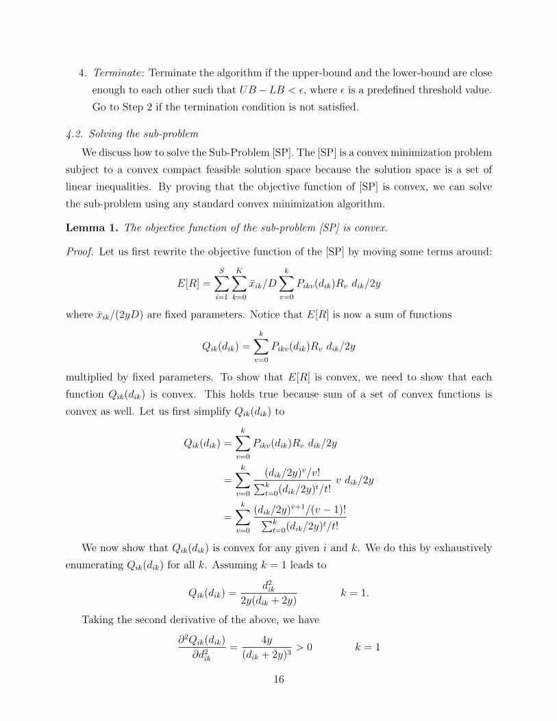
4.2. Solving the sub-problem
We discuss how to solve the Sub-Problem [SP]. The [SP] is a convex minimization problem
subject to a convex compact feasible solution space because the solution space is a set of
linear inequalities. By proving that the objective function of [SP] is convex, we can solve
the sub-problem using any standard convex minimization algorithm.
Lemma 1. The objective function of the sub-problem [SP] is convex.
Proof. Let us first rewrite the objective function of the [SP] by moving some terms around:
E[R] =S∑
i=1
K∑k=0
xik/Dk∑
v=0
Pikv(dik)Rv dik/2y
where xik/(2yD) are fixed parameters. Notice that E[R] is now a sum of functions
Qik(dik) =k∑
v=0
Pikv(dik)Rv dik/2y
multiplied by fixed parameters. To show that E[R] is convex, we need to show that each
function Qik(dik) is convex. This holds true because sum of a set of convex functions is
convex as well. Let us first simplify Qik(dik) to
Qik(dik) =k∑
v=0
Pikv(dik)Rv dik/2y
=k∑
v=0
(dik/2y)v/v!∑kt=0(dik/2y)t/t!
v dik/2y
=k∑
v=0
(dik/2y)v+1/(v − 1)!∑kt=0(dik/2y)t/t!
We now show that Qik(dik) is convex for any given i and k. We do this by exhaustively
enumerating Qik(dik) for all k. Assuming k = 1 leads to
Qik(dik) =d2ik
2y(dik + 2y)k = 1.
Taking the second derivative of the above, we have
∂2Qik(dik)
∂d2ik=
4y
(dik + 2y)3> 0 k = 1
16
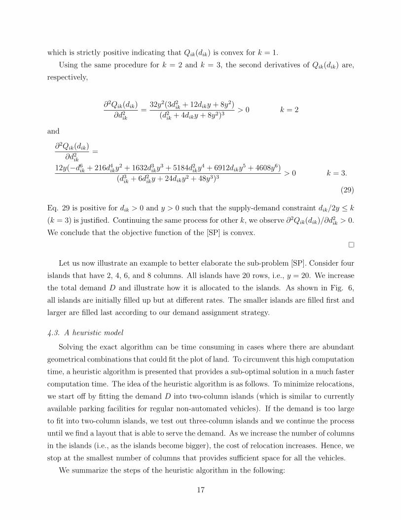
which is strictly positive indicating that Qik(dik) is convex for k = 1.
Using the same procedure for k = 2 and k = 3, the second derivatives of Qik(dik) are,
respectively,
∂2Qik(dik)
∂d2ik=
32y2(3d2ik + 12diky + 8y2)
(d2ik + 4diky + 8y2)3> 0 k = 2
and
∂2Qik(dik)
∂d2ik=
12y(−d6ik + 216d4iky2 + 1632d3iky
3 + 5184d2iky4 + 6912diky
5 + 4608y6)
(d3ik + 6d2iky + 24diky2 + 48y3)3> 0 k = 3.
(29)
Eq. 29 is positive for dik > 0 and y > 0 such that the supply-demand constraint dik/2y ≤ k
(k = 3) is justified. Continuing the same process for other k, we observe ∂2Qik(dik)/∂d2ik > 0.
We conclude that the objective function of the [SP] is convex.
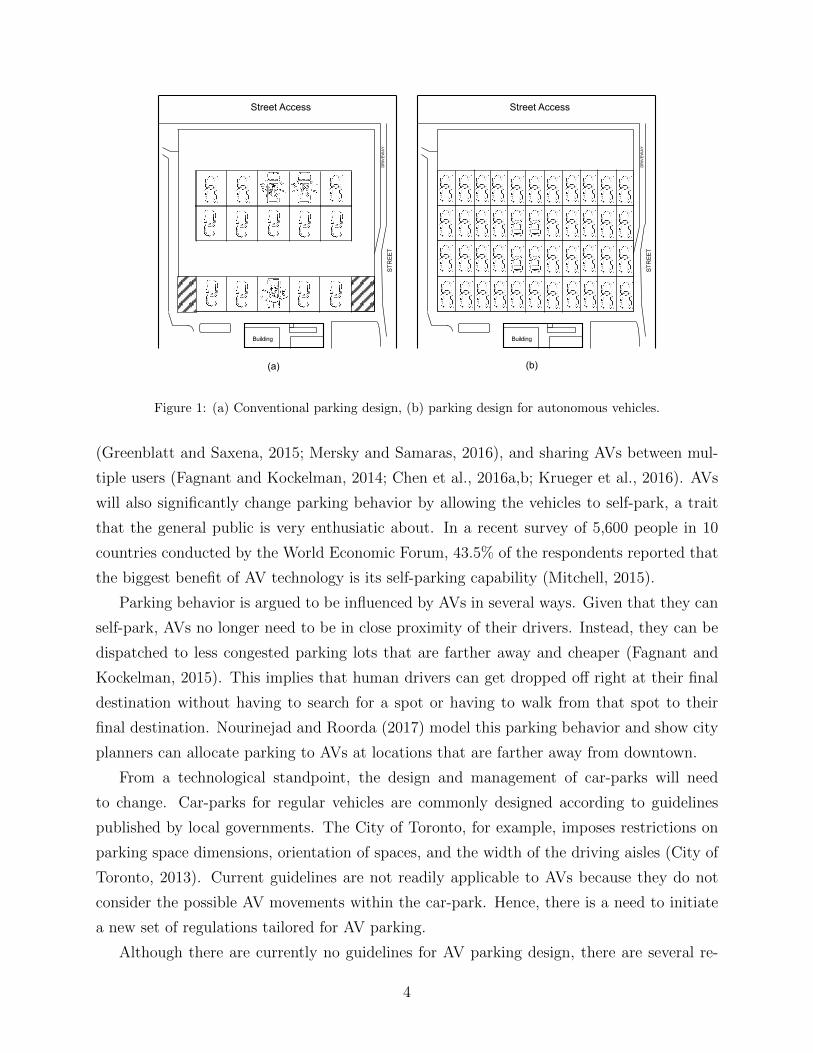
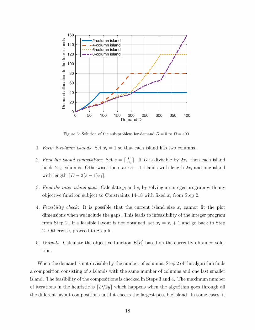
Let us now illustrate an example to better elaborate the sub-problem [SP]. Consider four
islands that have 2, 4, 6, and 8 columns. All islands have 20 rows, i.e., y = 20. We increase
the total demand D and illustrate how it is allocated to the islands. As shown in Fig. 6,
all islands are initially filled up but at different rates. The smaller islands are filled first and
larger are filled last according to our demand assignment strategy.
4.3. A heuristic model
Solving the exact algorithm can be time consuming in cases where there are abundant
geometrical combinations that could fit the plot of land. To circumvent this high computation
time, a heuristic algorithm is presented that provides a sub-optimal solution in a much faster
computation time. The idea of the heuristic algorithm is as follows. To minimize relocations,
we start off by fitting the demand D into two-column islands (which is similar to currently
available parking facilities for regular non-automated vehicles). If the demand is too large
to fit into two-column islands, we test out three-column islands and we continue the process
until we find a layout that is able to serve the demand. As we increase the number of columns
in the islands (i.e., as the islands become bigger), the cost of relocation increases. Hence, we
stop at the smallest number of columns that provides sufficient space for all the vehicles.
We summarize the steps of the heuristic algorithm in the following:
17
Demand D0 50 100 150 200 250 300 350 400
Dem
and
allo
catio
n to
the
four
isla
nds
0
20
40
60
80
100
120
140
1602-column island4-column island6-column island8-column island
Figure 6: Solution of the sub-problem for demand D = 0 to D = 400.
1. Form 2-column islands : Set xi = 1 so that each island has two columns.
2. Find the island composition: Set s = d D2xie. If D is divisible by 2xi, then each island
holds 2xi columns. Otherwise, there are s − 1 islands with length 2xi and one island
with length dD − 2(s− 1)xie.
3. Find the inter-island gaps : Calculate gi and ei by solving an integer program with any
objective funciton subject to Constraints 14-18 with fixed xi from Step 2.
4. Feasibility check : It is possible that the current island size xi cannot fit the plot
dimensions when we include the gaps. This leads to infeasibility of the integer program
from Step 2. If a feasible layout is not obtained, set xi = xi + 1 and go back to Step
2. Otherwise, proceed to Step 5.
5. Outputs : Calculate the objective function E[R] based on the currently obtained solu-
tion.
When the demand is not divisible by the number of columns, Step 2 of the algorithm finds
a composition consisting of s islands with the same number of columns and one last smaller
island. The feasibility of the compositions is checked in Steps 3 and 4. The maximum number
of iterations in the heuristic is dD/2ye which happens when the algorithm goes through all
the different layout compositions until it checks the largest possible island. In some cases, it
18
is possible that no feasible layout is obtained in the heuristic algorithm because the heuristic
only checks a subset of the entire solution space. In such cases, the exact algorithm provides
the only solution to the problem.
4.4. Measures of effectiveness
We present the following measures to assess and compare the results of the model. The
measures of effectiveness are the following:
• Expected relocations : This is the primary measure indicating the number of relocations
per vehicle retrieval, i.e., the objective function of [LD].
• Parking supply : Parking supply is the number of spots in all islands to serve a given
demand D.
• Utilization: Utilization is the ratio of the total area allocated to the islands over the
area of the entire plot of land. It is clear that utilization is never equal to 1 because
some of the land is allocated to the gaps and the clearance roadway. It is also clear
that utilization increases with demand because the operator has turn more of the plot
into islands.
• Maximum demand : Maximum demand Dmax is the largest demand that can be served
by a given plot of land. To find Dmax, we increase the demand D incrementally to
the point where the exact algorithm can no longer find a feasible solution to serve the
demand.
• Spatial efficiency ratio: This measure is the ratio of Dmax over the maximum pos-
sible demand if we only have 2-column islands. Informally, this ratio indicates the
economic benefit of turning existing conventional car-parks for regular vehicles into
fully-automated AV parking facilities. As an example, a spatial efficiency ratio of 2
indicates that we can fit twice as many AVs than regular vehicles in the same parking
facility. For the 2-column islands we use spot dimensions l = 5 and w = 2.8 which are
the parking dimensions of a regular vehicle. For AV parking spots, we use l = 5 and
w = 2.
5. Numerical experiments
We perform the following numerical experiments to gain managerial insights on AV park-
ing operations and to assess the computational efficiency and accuracy of two solution al-
gorithms. Except stated otherwise, we have used the exact algorithm with a termination
19
threshold ε = 0.05 to solve the instances. To solve the Master-Problem integer program,
we use the ILOG CPLEX package. For the sub-problem, we use a Sequential Quadratic
Programming algorithm to find the optimal solution.
5.1. Parking demand
Consider a parking facility with dimensions L = 150[m], W = 65[m], l = 5[m], and
w = 2[m]. There are y = 30 rows in each island and the width of the clearance roadway is
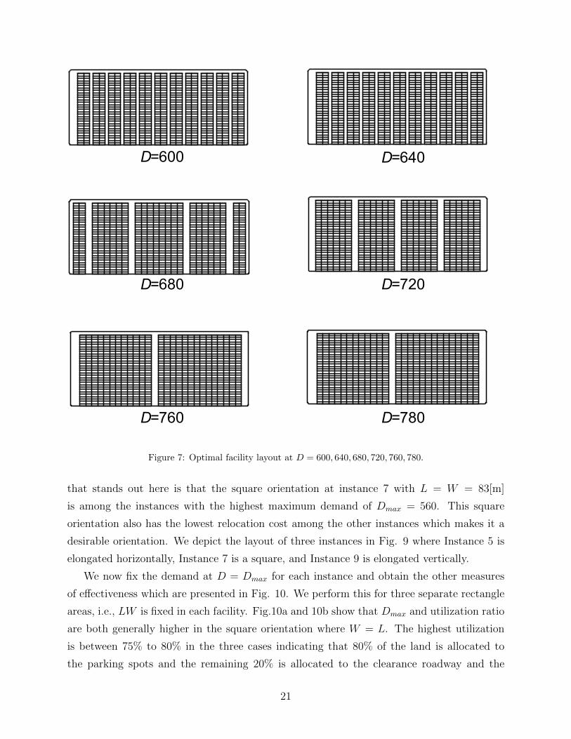
5[m]. We increase the demand from D = 600[veh] to D = 780[veh] and depict the geometrical
shape of the optimal facility in Fig. 7. When the demand is low, the islands all have only
two columns which is very similar to existing parking facilities for regular vehicles. The two-
column design has the lowest relocation cost and is desirable when demand is low to medium.
As the demand increases, the islands become bigger with more columns. The two-column
islands are eliminated at the largest demands because these islands require gaps that takes
up valuable land that could otherwise be used as island space. The maximum demand Dmax
that the facility can serve is 780 [veh]. The parking supply in the six instances is 660, 660,
720, 720, 780, and 780, respectively.
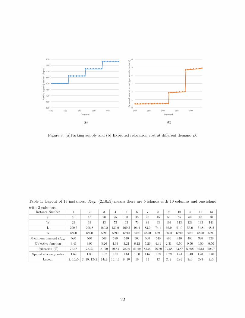
We present the parking supply (i.e., number of spots) and relocation cost (i.e. E[R])
with respect to demand in Fig. 8. It is shown that parking supply increases in a step-wise
fashion. The points where the steps occur are the points where the layout of the facility
changes radically. For instance, from D = 0 to D = 660, the optimal layout is 11 two-
column islands as shown in Fig. 7 (D = 600) with the demand is evenly distributed between
the islands. At D = 661, however, the car-park layout changes radically which leads to a
jump in parking supply. Fig. 8 illustrates that for the highest demand D = 780 [veh], we
need to approximately relocate 5 vehicles at any random retrieval.
For expected relocations E[R], we see the same step-wise jumps where the radical layout
changes occur. However, there is also a gradual increase in every step which is intuitive as a
higher demand requires more relcoations. The insight here is that operators need to choose
their design demand D while considering the jumps in the relocation cost since a marginal
decrease in D can substantially reduce the relocation cost.
5.2. Maximum demand
The maximum demand Dmax depends on the area and dimensions of the parking facility.
We present 13 parking facility dimensions in Table 1. The instances have different length L
and width W but their area is fixed, i.e., LW = 6890[m2] is constant. The highest maximum
demand is Dmax = 560 which occurs in the square orientation with L ≈ W . An observation
20
D=600 D=640
D=680 D=720
D=760 D=780
Figure 7: Optimal facility layout at D = 600, 640, 680, 720, 760, 780.
that stands out here is that the square orientation at instance 7 with L = W = 83[m]
is among the instances with the highest maximum demand of Dmax = 560. This square
orientation also has the lowest relocation cost among the other instances which makes it a
desirable orientation. We depict the layout of three instances in Fig. 9 where Instance 5 is
elongated horizontally, Instance 7 is a square, and Instance 9 is elongated vertically.
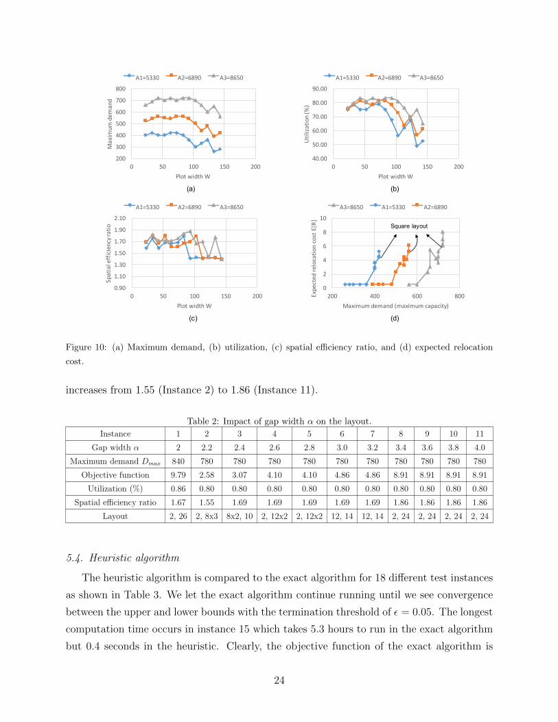
We now fix the demand at D = Dmax for each instance and obtain the other measures
of effectiveness which are presented in Fig. 10. We perform this for three separate rectangle
areas, i.e., LW is fixed in each facility. Fig.10a and 10b show that Dmax and utilization ratio
are both generally higher in the square orientation where W = L. The highest utilization
is between 75% to 80% in the three cases indicating that 80% of the land is allocated to
the parking spots and the remaining 20% is allocated to the clearance roadway and the
21
400
450
500
550
600
650
700
750
800
540 590 640 690 740
Parkingsupply(num
berofsp
ots)
Demand
0
1
2
3
4
5
6
540 590 640 690 740
Expectedrelocationcost(p
ervehicleretrieval)
Demand
(a) (b)
Figure 8: (a)Parking supply and (b) Expected relocation cost at different demand D.
Table 1: Layout of 13 instances. Key : (2,10x5) means there are 5 islands with 10 columns and one island
with 2 columns.Instance Number 1 2 3 4 5 6 7 8 9 10 11 12 13
y 10 15 20 25 30 35 40 45 50 55 60 65 70
W 23 33 43 53 63 73 83 93 103 113 123 133 143
L 299.5 208.8 160.2 130.0 109.3 94.4 83.0 74.1 66.9 61.0 56.0 51.8 48.2
A 6890 6890 6890 6890 6890 6890 6890 6890 6890 6890 6890 6890 6890
Maximum demand Dmax 520 540 560 550 540 560 560 540 500 440 480 390 420
Objective function 3.46 3.96 5.26 4.03 3.21 6.12 5.26 4.41 2.31 0.50 0.50 0.50 0.50
Utilization (%) 75.48 78.39 81.29 79.84 78.39 81.29 81.29 78.39 72.58 63.87 69.68 56.61 60.97
Spatial efficiency ratio 1.69 1.80 1.67 1.80 1.61 1.60 1.67 1.69 1.79 1.41 1.43 1.41 1.40
Layout 2, 10x5 2, 10, 12x2 14x2 10, 12 8, 10 16 14 12 2, 8 2x4 2x4 2x3 2x3
22
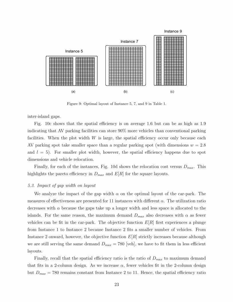
Instance 5
Instance 7
Instance 9
(a) (b) (c)
Figure 9: Optimal layout of Instance 5, 7, and 9 in Table 1.
inter-island gaps.
Fig. 10c shows that the spatial efficiency is on average 1.6 but can be as high as 1.9
indicating that AV parking facilities can store 90% more vehicles than conventional parking
facilities. When the plot width W is large, the spatial efficiency occur only because each
AV parking spot take smaller space than a regular parking spot (with dimensions w = 2.8
and l = 5). For smaller plot width, however, the spatial efficiency happens due to spot
dimensions and vehicle relocation.
Finally, for each of the instances, Fig. 10d shows the relocation cost versus Dmax. This
highlights the pareto efficiency in Dmax and E[R] for the square layouts.
5.3. Impact of gap width on layout
We analyze the impact of the gap width α on the optimal layout of the car-park. The
measures of effectiveness are presented for 11 instances with different α. The utilization ratio
decreases with α because the gaps take up a longer width and less space is allocated to the
islands. For the same reason, the maximum demand Dmax also decreases with α as fewer
vehicles can be fit in the car-park. The objective function E[R] first experiences a plunge
from Instance 1 to Instance 2 because Instance 2 fits a smaller number of vehicles. From
Instance 2 onward, however, the objective function E[R] strictly increases because although
we are still serving the same demand Dmax = 780 [veh], we have to fit them in less efficient
layouts.
Finally, recall that the spatial efficiency ratio is the ratio of Dmax to maximum demand
that fits in a 2-column design. As we increase α, fewer vehicles fit in the 2-column design
but Dmax = 780 remains constant from Instance 2 to 11. Hence, the spatial efficiency ratio
23
200
300
400
500
600
700
800
0 50 100 150 200
Maxim
umdem
and
PlotwidthW
A1=5330 A2=6890 A3=8650
40.00
50.00
60.00
70.00
80.00
90.00
0 50 100 150 200
Utilization(%
)
PlotwidthW
A1=5330 A2=6890 A3=8650
0
2
4
6
8
10
200 400 600 800Expectedre
locatio
ncostE[R]
Maximumdemand(maximumcapacity)
A3=8650 A1=5330 A2=6890
(a) (b)
(c) (d)
Square layout
0.90
1.10
1.30
1.50
1.70
1.90
2.10
0 50 100 150 200
Spatialefficiencyratio
PlotwidthW
A1=5330 A2=6890 A3=8650
Figure 10: (a) Maximum demand, (b) utilization, (c) spatial efficiency ratio, and (d) expected relocation
cost.
increases from 1.55 (Instance 2) to 1.86 (Instance 11).
Table 2: Impact of gap width α on the layout.
Instance 1 2 3 4 5 6 7 8 9 10 11
Gap width α 2 2.2 2.4 2.6 2.8 3.0 3.2 3.4 3.6 3.8 4.0
Maximum demand Dmax 840 780 780 780 780 780 780 780 780 780 780
Objective function 9.79 2.58 3.07 4.10 4.10 4.86 4.86 8.91 8.91 8.91 8.91
Utilization (%) 0.86 0.80 0.80 0.80 0.80 0.80 0.80 0.80 0.80 0.80 0.80
Spatial efficiency ratio 1.67 1.55 1.69 1.69 1.69 1.69 1.69 1.86 1.86 1.86 1.86
Layout 2, 26 2, 8x3 8x2, 10 2, 12x2 2, 12x2 12, 14 12, 14 2, 24 2, 24 2, 24 2, 24
5.4. Heuristic algorithm
The heuristic algorithm is compared to the exact algorithm for 18 different test instances
as shown in Table 3. We let the exact algorithm continue running until we see convergence
between the upper and lower bounds with the termination threshold of ε = 0.05. The longest
computation time occurs in instance 15 which takes 5.3 hours to run in the exact algorithm
but 0.4 seconds in the heuristic. Clearly, the objective function of the exact algorithm is
24
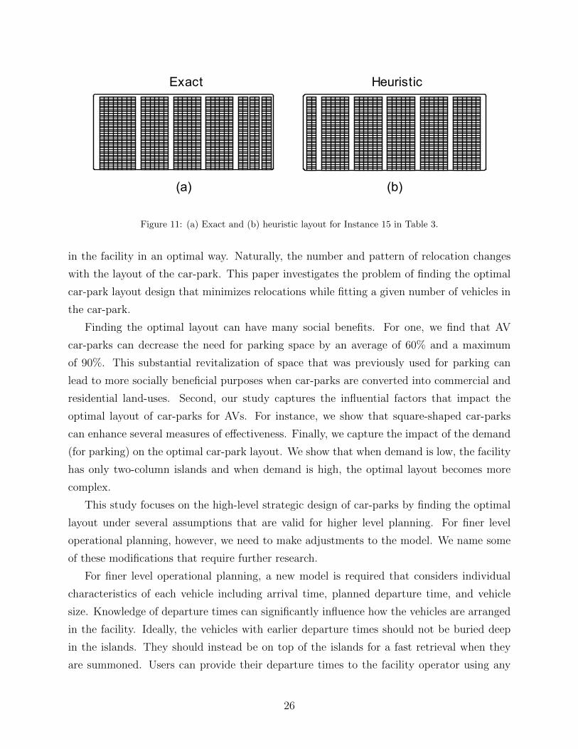
always lower or at least equal to the heuristic. In Instance 1, we observe that the exact
algorithm’s objective function is 18% lower than the heuristic. This happens as the heuristic
fully fills up 13 two-column islands (until the entire demand allocated) whereas the exact
partially fills up 15 two-column islands. Hence, the heuristic is not strong in exploring cases
of partial filling. In Instance 17, we also observe a 15% difference in objective functions
because the exact is able to explore a wider range of possible layout compositions compared
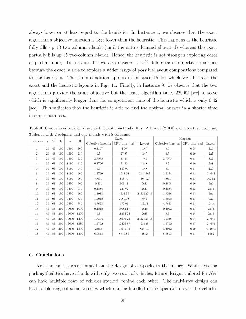
to the heuristic. The same condition applies in Instance 15 for which we illustrate the
exact and the heuristic layouts in Fig. 11. Finally, in Instance 9, we observe that the two
algorithms provide the same objective but the exact algorithm takes 229.62 [sec] to solve
which is significantly longer than the computation time of the heuristic which is only 0.42
[sec]. This indicates that the heuristic is able to find the optimal answer in a shorter time
in some instances.
Table 3: Comparison between exact and heuristic methods. Key: A layout (2x3,8) indicates that there are
3 islands with 2 columns and one islands with 8 columns.
Instances y W L A DExact Heuristic
Objective function CPU time [sec] Layout Objective function CPU time [sec] Layout
1 20 43 100 4300 200 0.4167 4.96 2x7 0.5 0.38 2x5
2 20 43 100 4300 280 0.5 27.85 2x7 0.5 0.40 2x7
3 20 43 100 4300 320 2.7573 13.44 8x2 2.7573 0.41 8x2
4 30 63 130 8190 480 0.4706 71.40 2x9 0.5 0.40 2x8
5 30 63 130 8190 540 0.5 159.05 2x9 0.5 0.41 2x9
6 30 63 130 8190 600 1.3769 1211.08 2x4, 6x2 1.8154 0.42 2, 6x3
7 30 63 130 8190 660 4.031 118.85 10, 12 4.031 0.43 10, 12
8 30 63 150 9450 500 0.431 303.31 2x11 0.4808 0.40 2x9
9 30 63 150 9450 630 0.4884 229.62 2x11 0.4884 0.42 2x11
10 30 63 150 9450 690 1.8983 4523.56 2x2, 6x2, 8 1.9236 0.43 6x4
11 30 63 150 9450 720 1.9615 2065.08 6x4 1.9615 0.43 6x4
12 30 63 150 9450 750 4.7623 472.06 12,14 4.7623 0.53 12,14
13 40 83 200 16600 1000 0.4545 13082.17 2x15 0.4902 0.43 2x13
14 40 83 200 16600 1200 0.5 11254.24 2x15 0.5 0.45 2x15
15 40 83 200 16600 1240 1.7804 18956.23 2x3, 6x3, 8 1.839 0.54 2, 6x5
16 40 83 200 16600 1280 1.8702 12426.87 2, 6x5 1.8702 0.47 2, 6x5
17 40 83 200 16600 1360 2.998 10951.65 8x3, 10 3.2962 0.49 4, 10x3
18 40 83 200 16600 1440 6.9813 6740.86 18x2 6.9813 0.51 18x2
6. Conclusions
AVs can have a great impact on the design of car-parks in the future. While existing
parking facilities have islands with only two rows of vehicles, future designs tailored for AVs
can have multiple rows of vehicles stacked behind each other. The multi-row design can
lead to blockage of some vehicles which can be handled if the operator moves the vehicles
25
Exact Heuristic
(a) (b)
Figure 11: (a) Exact and (b) heuristic layout for Instance 15 in Table 3.
in the facility in an optimal way. Naturally, the number and pattern of relocation changes
with the layout of the car-park. This paper investigates the problem of finding the optimal
car-park layout design that minimizes relocations while fitting a given number of vehicles in
the car-park.
Finding the optimal layout can have many social benefits. For one, we find that AV
car-parks can decrease the need for parking space by an average of 60% and a maximum
of 90%. This substantial revitalization of space that was previously used for parking can
lead to more socially beneficial purposes when car-parks are converted into commercial and
residential land-uses. Second, our study captures the influential factors that impact the
optimal layout of car-parks for AVs. For instance, we show that square-shaped car-parks
can enhance several measures of effectiveness. Finally, we capture the impact of the demand
(for parking) on the optimal car-park layout. We show that when demand is low, the facility
has only two-column islands and when demand is high, the optimal layout becomes more
complex.
This study focuses on the high-level strategic design of car-parks by finding the optimal
layout under several assumptions that are valid for higher level planning. For finer level
operational planning, however, we need to make adjustments to the model. We name some
of these modifications that require further research.
For finer level operational planning, a new model is required that considers individual
characteristics of each vehicle including arrival time, planned departure time, and vehicle
size. Knowledge of departure times can significantly influence how the vehicles are arranged
in the facility. Ideally, the vehicles with earlier departure times should not be buried deep
in the islands. They should instead be on top of the islands for a fast retrieval when they
are summoned. Users can provide their departure times to the facility operator using any
26
smart platforms such as a mobile app.
In the model, we assumed that parking demand is constant and fixed throughout the
planning period which led to one optimal layout for the parking facility. In practice, however,
this optimal layout can change within the day according to dynamic parking demand. For
example, the facility can have one layout in the morning and another layout in the afternoon.
As a future research, it is valuable to derive the optimal dynamic layout of the facility
according to changes in demand.
We present a model for cases where the facility plot is a rectangle with given dimensions.
A clear-cut rectangular plot may not always exist in reality. Hence, it is important to extend
the model to solve other irregular plot profiles as well. It is also important to consider the
optimal layout in multi-storey buildings where the floors are connected either through a
elevators (for vehicles) or ramps.
References
Anjos, M. F., Vieira, M. V., 2017. Mathematical optimization approaches for facility lay-
out problems: The state-of-the-art and future research directions. European Journal of
Operational Research.
Boyles, S. D., Tang, S., Unnikrishnan, A., 2015. Parking search equilibrium on a network.
Transportation Research Part B: Methodological 81, 390–409.
Chen, T. D., Kockelman, K. M., Hanna, J. P., 2016a. Operations of a shared, autonomous,
electric vehicle fleet: implications of vehicle & charging infrastructure decisions. Trans-
portation Research Part A,(under review for publication).
Chen, Z., He, F., Zhang, L., Yin, Y., 2016b. Optimal deployment of autonomous vehicle
lanes with endogenous market penetration. Transportation Research Part C: Emerging
Technologies 72, 143–156.
Chester, M., Horvath, A., Madanat, S., 2011. Parking infrastructure and the environment.
ACCESS Magazine 1 (39).
City of Toronto, 2013. City of toronto zoning by-law.
de Almeida Correia, G. H., van Arem, B., 2016. Solving the user optimum privately owned
automated vehicles assignment problem (uo-poavap): A model to explore the impacts of
self-driving vehicles on urban mobility. Transportation Research Part B: Methodological
87, 64–88.
27
De Castilho, B., Daganzo, C. F., 1993. Handling strategies for import containers at marine
terminals. University of California Transportation Center.
de Oliveira, I. R., 2017. Analyzing the performance of distributed conflict resolution among
autonomous vehicles. Transportation Research Part B: Methodological 96, 92–112.
DesignBoom, 2015. Audi urban future initiative brings automated parking garage for
self-driving cars to boston-area.
URL http://www.designboom.com/design/audi-urban-future-initiative-11-20-2015/
Fagnant, D. J., Kockelman, K., 2015. Preparing a nation for autonomous vehicles: opportu-
nities, barriers and policy recommendations. Transportation Research Part A: Policy and
Practice 77, 167–181.
Fagnant, D. J., Kockelman, K. M., 2014. The travel and environmental implications of shared
autonomous vehicles, using agent-based model scenarios. Transportation Research Part C:
Emerging Technologies 40, 1–13.
Gallivan, S., 2011. Ibm global parking survey: Drivers share worldwide parking woes. IBM,
September 18.
Goncalves, J. F., Resende, M. G., 2015. A biased random-key genetic algorithm for the
unequal area facility layout problem. European Journal of Operational Research 246 (1),
86–107.
Greenblatt, J. B., Saxena, S., 2015. Autonomous taxis could greatly reduce greenhouse-gas
emissions of us light-duty vehicles. nature climate change 5 (9), 860–863.
He, F., Yin, Y., Chen, Z., Zhou, J., 2015. Pricing of parking games with atomic players.
Transportation Research Part B: Methodological 73, 1–12.
Hungerlander, P., Anjos, M. F., 2015. A semidefinite optimization-based approach for global
optimization of multi-row facility layout. European journal of operational Research 245 (1),
46–61.
Jiang, X. J., Jin, J. G., 2017. A branch-and-price method for integrated yard crane deploy-
ment and container allocation in transshipment yards. Transportation Research Part B:
Methodological 98, 62–75.
28
Kalra, N., Paddock, S. M., 2016. Driving to safety: How many miles of driving would it take
to demonstrate autonomous vehicle reliability? Transportation Research Part A: Policy
and Practice 94, 182–193.
Katrakazas, C., Quddus, M., Chen, W.-H., Deka, L., 2015. Real-time motion planning meth-
ods for autonomous on-road driving: State-of-the-art and future research directions. Trans-
portation Research Part C: Emerging Technologies 60, 416–442.
Krueger, R., Rashidi, T. H., Rose, J. M., 2016. Preferences for shared autonomous vehicles.
Transportation research part C: emerging technologies 69, 343–355.
Larson, R. C., Odoni, A. R., 1981. Urban operations research. No. Monograph.
Le Vine, S., Zolfaghari, A., Polak, J., 2015. Autonomous cars: the tension between oc-
cupant experience and intersection capacity. Transportation Research Part C: Emerging
Technologies 52, 1–14.
Lei, C., Ouyang, Y., 2017. Dynamic pricing and reservation for intelligent urban parking
management. Transportation Research Part C: Emerging Technologies 77, 226–244.
Levin, M. W., Boyles, S. D., 2016. A cell transmission model for dynamic lane reversal
with autonomous vehicles. Transportation Research Part C: Emerging Technologies 68,
126–143.
Liu, W., Geroliminis, N., 2016. Modeling the morning commute for urban networks with
cruising-for-parking: An mfd approach. Transportation Research Part B: Methodological
93, 470–494.
Mahmassani, H. S., 2016. 50th anniversary invited articleautonomous vehicles and connected
vehicle systems: Flow and operations considerations. Transportation Science 50 (4), 1140–
1162.
Mersky, A. C., Samaras, C., 2016. Fuel economy testing of autonomous vehicles. Transporta-
tion Research Part C: Emerging Technologies 65, 31–48.
Mitchell, A., 2015. Are we ready for self-driving cars? World Economic Forum.
Nourinejad, M., Roorda, M. J., 2017. The end of cruising for parking in the era of autonomous
vehicles. Under review.
29
Pel, A. J., Chaniotakis, E., 2017. Stochastic user equilibrium traffic assignment with equili-
brated parking search routes. Transportation Research Part B: Methodological 101, 123–
139.
Shao, C., Yang, H., Zhang, Y., Ke, J., 2016. A simple reservation and allocation model of
shared parking lots. Transportation Research Part C: Emerging Technologies 71, 303–312.
South China Morning Post, 2015. Price volatility high for hong kong parking spaces.
Talebpour, A., Mahmassani, H. S., 2016. Influence of connected and autonomous vehicles
on traffic flow stability and throughput. Transportation Research Part C: Emerging Tech-
nologies 71, 143–163.
TechWorld , 2016. The huge impact driverless cars will have on parking and urban landscapes.
Thompson, C., 2016. No parking here.
Waymo, 2016. On the road.
URL https://waymo.com/ontheroad/
Yang, B., Monterola, C., 2016. Efficient intersection control for minimally guided vehicles:
A self-organised and decentralised approach. Transportation Research Part C: Emerging
Technologies 72, 283–305.
Zhang, C., Wan, Y.-w., Liu, J., Linn, R. J., 2002. Dynamic crane deployment in container
storage yards. Transportation Research Part B: Methodological 36 (6), 537–555.
30


