
DESIGN AND EVALUATION OF A TEST PLATFROM FOR THERMAL MECHANICAL AND ACOUSTICAL
LOADING
by
ABDI JASMIN
A thesis submitted in fulfillment of the requirements for the Honors in the Major Program in Mechanical Engineering
in the College of Engineering and Computer Science and the Burnett Honors College
at the University of Central Florida Orlando, Florida
Spring Term, 2015
Thesis Chair: Ali P. Gordon, Ph.D.

Abstract
A test device for thermal, mechanical, and acoustical loading has been designed to replicate
the combined extreme environment to which hypersonic fuselage components are exposed. The
fuselage panels are typically subjected to super-imposed cycling from hypersonic
shock/impingement and aerodynamic pressure from the usual ascent-cruise-decent mission profile
of the aircraft combined with mechanical vibration at acoustic frequencies; moreover, these slender
components will undergo conventional mechanical fatigue with compressive mean stress due to
geometric constraint. A universal column buckling frame, an acoustic horn, and a custom-made
quartz-lamp furnace is tuned via a GUI to allow users to design cyclic load profiles that idealize
the thermo-acousto-mechanical loading of critical panels.
ii

Acknowledgement I would like to express the deepest appreciation to my committee chair Dr. Ali Gordon,
who has shown the attitude and the substance of a genius: he continually and persuasively conveyed a spirit of adventure in regard to research and scholarship, and an excitement in regard
to mentoring. Without his supervision and constant help this dissertation would not have been possible.
I would like to thank my committee members, Dr. Kuo-Chi ‘Kurt’ Lin and Dr. Necati Catbas for their support. In addition, a thank you to the Brunet Honors College for their financial
support granted through the Honor in the Major Scholarship.
iii

Table of Contents
Abstract ........................................................................................................................................... ii
Acknowledgement ......................................................................................................................... iii Table of Contents ........................................................................................................................... iv
List of Figures ................................................................................................................................ vi
List of Tables ................................................................................................................................ vii
Nomenclature ............................................................................................................................... viii Chapter 1. Introduction ............................................................................................................... 1
Motivation ................................................................................................................................... 1
Overview ..................................................................................................................................... 2
Chapter 2. Background ............................................................................................................... 4
Eulerian Buckling ........................................................................................................................ 4
Column Buckling Experiments ................................................................................................... 9
Post Buckling Response ............................................................................................................ 11
Chapter 3. Experimental Approach .......................................................................................... 13
Test Requirements ..................................................................................................................... 13
Test device Design .................................................................................................................... 14
Device Performance .................................................................................................................. 19
Mechanical ............................................................................................................................ 19
Thermal ................................................................................................................................. 22
Acoustical ............................................................................................................................. 22
Test Material ............................................................................................................................. 24
Mechanical Model ..................................................................................................................... 25
Chapter 4. Results ..................................................................................................................... 27
Mechanical ................................................................................................................................ 27
Thermal ...................................................................................... Error! Bookmark not defined.
Acoustical ................................................................................... Error! Bookmark not defined.
Combined .................................................................................................................................. 27
Chapter 5. Numerical Simulations............................................................................................ 28
Specimen Model ........................................................................................................................ 28
iv

Finite Element Model ................................................................................................................ 29
Results ....................................................................................................................................... 31
Chapter 6. Comparisons and Observations............................................................................... 33
Chapter 7. Conclusion .............................................................................................................. 33
References ..................................................................................................................................... 34
v

List of Figures
Figure 1 Critical panels of the DARPA Falcon HTV-3X designed for Mach 5.2. ......................... 1 Figure 2 Graphical user interface developed in LabView .............................................................. 3 Figure 3 Stout vs slender component under compressive force P .................................................. 4 Figure 4 Slender column under bi-clamped boundary condition................................................... 5 Figure 5 Bi-clamped simulation of AISA 304 beam E=27.5e6 psi with dimensions L=0.4m, b=25.4mm, a=2.29mm, P=1.3KN. .................................................................................................. 8 Figure 6 the effect of eccentricity on critical buckling load ........................................................... 9 Figure 7 - Post buckling deformation response of steel. ............................................................... 12 Figure 8 – Bi-clamped testing condition of a 0.41m long specimen. ........................................... 13 Figure 9 Reconfiguration of the Sanderson frame ........................................................................ 14 Figure 10 Load Cell Calibration ................................................................................................... 15 Figure 11 Furnace triangular design ............................................................................................. 16 Figure 12 Thermocouple settings for temperature profile and PID control .................................. 17 Figure 13 Horn assembly on 8020 frame ...................................................................................... 17 Figure 14 Accelerometers on sample ............................................................................................ 18 Figure 15 Platform for Combine Extreme Environments (P-CEEn): (a) numerical model and (b) physical device with test specimen ............................................................................................... 19 Figure 16 Initial load- and displacement-controlled deformation response of specimen A2 ....... 20 Figure 17 Cycle load Pmax=190N, Pcr=1014N, L=0.4572 ............................................................. 21 Figure 18 8 consecutive and consistent cycles ............................................................................. 21 Figure 19 Furnace performance .................................................................................................... 22 Figure 20 Acoustic transfer efficiency .......................................................................................... 23 Figure 21 Specimen used in the initial phase................................................................................ 23 Figure 22 Southwell Plot .............................................................................................................. 26 Figure 23 Software used for simulation ........................................................................................ 28 Figure 24 Specimen CAD and dimensions ................................................................................... 28 Figure 25 Fixed geometry feature ................................................................................................. 29 Figure 26 Roller/Sider feature ...................................................................................................... 30 Figure 27 Load being applied to the specimen ............................................................................. 30 Figure 28 Final FEM model for buckling analysis ....................................................................... 30 Figure 29 Buckling analysis of specimen S28 .............................................................................. 31 Figure 30 Buckling analysis of specimen S30 .............................................................................. 32 Figure 31 Buckling analysis of specimen S32 .............................................................................. 33
vi

List of Tables
Table 1 Specimen dimensions and properties ............................................................................... 25 Table 2 Buckling analysis simulation ........................................................................................... 33
vii

Nomenclature
δH = Horizontal deflection [mm] δV = Vertical deflection [mm] tc = Compressive dwell period [s] tcyc = Cycle time [s] A = Cross-sectional area [mm2] fa = Acoustic frequency [Hz or s-1] I = Moment of inertia [mm4] P = Compressive Load [kN] E = Young’s Modulus [GPa] L = Length of specimen [m] b = Specimen width [mm] a = Specimen thickness [mm] SPL = Acoustic Pressure [dB] ∆T = Temperature Range [°C] T = Temperature [°C] t = time [s]
viii

Chapter 1. Introduction
Motivation
Figure 1 Critical panels of the DARPA Falcon HTV-3X designed for Mach 5.2.
Engineering materials normally do not reach theoretical strength when they are tested in the
laboratory. In service-like situations, components and structures are usually subjected to several
modes of loading simultaneously. These loads usually affect the strength, deformation, and life of
that object or structure in engineering applications. For example, vehicles for aerial combat (e.g.
F-22 Raptor, A-10 Thunderbolt II) during operational life will be subjected to various impacts that
might result in mechanical damage. An analogous land-based combined extreme environment case
would be railroad wheels under thermo-mechanical loading. Railroad wheels experience thermal
loading during brake shoe applications. Hot spots develop on the tread of the wheel as it passes
under the brake shoe. Thermal stresses on the hot spots are higher than the surrounding cooler
material. Oxide formation at the tread (hot spots) and flange regions may be extensive and
influence crack nucleation. The hot spots and other critical regions experience many small thermal
cycles within major thermal cycles [1]. A test platform capable of replicating the combined
extreme environment to which hypersonic fuselage components will be exposed has been
1

developed. In service, (1) thermal cycling load is developed on the components in combination
with (2) mechanical vibration at acoustic frequencies due to hypersonic shock/impingements and
aerodynamic pressure. Additionally, these relatively thin components will undergo conventional
(3) mechanical fatigue with compressive mean stress due to geometric constraints and maneuvers
of the vehicle; therefore, the test platform will simulate cycles of thermal, mechanical and acoustic
loads superimposed. Having the ability to precisely replicate the working environment of the
fuselage components will help to identify life limiting conditions of the materials. It is also an
effective method to determine the limits of the structure and make appropriate adjustments when
necessary.
Overview
This thesis continues with a review of recent literature relevant to this study in Chapter 2
and a brief background on buckling. Chapter 3 contains information on the experimental approach.
Once the test device had been developed, it was paired with a graphical user interface (Fig. 2)
developed in LabView. Several experiments were performed in order to calibrate the test device
before usage. The strength and the weaknesses of the device were identified and the device was
improved as needed.
2

Figure 2 Graphical user interface developed in LabView
3

Chapter 2. Background
A structural component such as a beam, a column or a rod subjected to a compressional load
would normally experience a deformation directly proportional to its length L and the load P and
inversely proportional to the young’s modulus E of the material. Ideally, a stout enough component
will deflect but remain untwisted similar to a coil spring subjected to an axial load and it is not
expected to fail (plasticized and flattened) at loads less than the compressive strength of the
material. However, if the loaded member is sufficiently slender (the ratio of its length L to its cross-
section dimension a is greater than ten), it will deflect and twist and eventually fail under a critical
load. This mechanical failure is known as buckling and it is presented in this chapter.
Figure 3 Stout vs slender component under compressive force P
Eulerian Buckling
Buckling, also known as structural instability, is a mechanical failure exhibited by a
sufficiently slender column (the ratio of its length L to its cross-section dimension a is greater than
ten) under compressive loading, P. It can be classified into two categories: (1) bifurcation bucking
or (2) limit load buckling [2]. Bifurcation buckling occurs when deflection under compressive load
goes from axial shortening to lateral deflection. The critical buckling load or simply critical load,
4

is the load at which the bifurcation occurs. The terms “primary path” and “secondary” (or “post
buckling path”) are used to describe the path that exists prior to and after bifurcation buckling. The
post buckling path is dependent of structure and loading. In limit load buckling, the structure
attains the maximum load without any previous bifurcation [3]. Other classification of buckling
are described with respect to the displacement magnitude or material behavior such as
elastic/inelastic buckling.
Figure 4 Slender column under bi-clamped boundary condition.
Euler was the first to study elastic stability using the theory of calculus of variations to
obtain the equilibrium equation and buckling load of a centrally compressed elastic column. For
uniform, perfectly straight, sufficiently slender (the ratio of the length to the cross-section
dimensions is greater than 10) and homogenous column as shown in Fig. 1, the theory of bending,
first suggested by Bernoulli, represents an accurate approximation to the exact solution according
to three-dimensional elasticity [4]. In his work, Euler has assumed that the cross section of the
column does not distort during buckling and. With column length, L, Young’s Modulus, E, and
5

second moment of inertia, I, subjected to an end axial compressive load P, the moment-
displacement relation according to the Euler-Bernoulli beam theory is given by
2
2
( )( ) d w xM x EIdx
= − (1)
Here ( )w x refers to the transverse displacement, and x is the longitudinal coordinate measured
from the column base. The cross bar refers to non-linearization by L (e.g. / , /w w L x x L= = ).
The theory is based on the assumption that plane normal cross-sections of the beam remain plane
and normal to the deflected centroidal axis of the beam, and the transverse normal stresses are
negligible. Equation (1) provides an essential characteristic of buckling: the failure load depends
primarily on the elastic modulus and the cross section stiffness of the material and is almost
independent of the material strength or yield limit [4]. In fact, slender columns generally buckle
prior to the exceedance of strength or stiffness criteria.
Analysis can be used to develop a deflection model and a critical load for buckling. The
general solution of the differential equation is expressed as
1 2 3 4( ) sin cosH x C x C x C x Cδ α α= + + + (2)
Whereα is equal to2PL
EI, and the constants 1 2 3, ,C C C and 4C are constants of integration. The
simplified solution for a bi-clamped case
( ) 1 cos xHM PxP EI
δ
= −
(3)
6

Here M in the constant moment developed at the end supports. It can be readily shown that the
critical buckling load is:
2
2
4cr
EIPLπ
= (4)
Hence, the critical buckling normal stress is given by
2
2
4( / )cr
EL rπσ = (5)
Where /r I A= is the radius of gyration, and /L r , is the slenderness ratio of column.
These equations are valid only for cases where the deformation can be assumed to be purely elastic
in an isothermal environment and under ideal conditions [5]. Figure 5 shows a numerically
simulated post buckling response of a slender 304 steel beam under longitudinal compression and
the horizontal displacement δH in millimeters. The sinusoidal deflection and fixed boundaries
predicted by Eq. (3) are verified. A load of 1.3KN was applied to the model and the resulting load
factor BLF=1. The buckling load factor (BLF) is the factor of safety against buckling or the ratio
of the buckling loads to the applied loads. BLF=1 means the applied loads are exactly equal to the
estimated critical loads, buckling is expected.
7

Figure 5 Bi-clamped simulation of AISA 304 beam E=27.5e6 psi with dimensions L=0.4m, b=25.4mm, a=2.29mm, P=1.3KN.
Up until now the structural member has been considered to be initially straight and loaded
along its neutral axis, but in reality, a structure and its loading will never match these idealizations.
That is one reason why materials normally do not reach theoretical strength when they are tested.
Small deviations from ideal can be assumed negligible when studying the behavior of structural
members such as beams, columns, shafts and rods under tension. However, they can make a
difference in determining elastic instabilities. Two types of imperfection that commonly occur
when studying buckling 1) load eccentricity, which occurs when the load applied P is at a distance
8

e from the neutral axis developing a moment M eP= and 2) the presence of an initial deflection
0δ . Figure 6 demonstrates how the critical buckling load will be affected by an increase of
eccentricity with respect to the length L.
Figure 6 the effect of eccentricity on critical buckling load
Column Buckling Experiments
In an effort to improve effectiveness and accuracy in predicting buckling and post buckling
strength, a variety of experiments have been performed. Carpinteri and collegues [6] investigated
the dependence of the fundamental frequency on the axial load in slender beams subjected to
imposed axial end displacements. Knowing that the presence of an initial curvature (geometrical
imperfection) of the beam axis can significantly affect the dynamic structural response of a slender
beam, they used equal length specimens with different initial curvatures in hinged–hinged and
hinged–clamped conditions. A servo-controlled machine (MTS) with a closed-loop electronic
control, having a maximum capacity of 100 kN. In order to apply vibration to the specimen, an
9

electromagnet positioned at mid-height of the tested beam transmitted a sinusoidal force to the
beam, controlled in frequency and amplitude by the wave generator. The time history of the beam
midpoint transversal displacement, measured with the laser sensor. Data such as (1) axial load with
respect to transverse displacement and (2) fundamental frequency versus axial load were generated
for analysis. The results were shown for frequencies ranging from 10Hz to 60Hz. They found that
a first phase, where the fundamental frequency decreases with the axial load, is followed by a
stiffening one, where the trend is reversed. The transition seems to be smoother with geometric
imperfection in the specimen.
The behavior of geometrically constrained columns has been studied in high temperature
environments [10], and it is well known that under a thermal load, the compressive load in a
column will increase due to thermal expansion. Furthermore, Wang indicates that increase in
temperature can cause degradation of strength and stiffness properties of a component [7].
Carpinteri confirms the existence of a relationship between the natural frequency and the stiffness
of the tested components [6].
Wang [7] investigated the local stability of steel stub columns at elevated temperatures.
The experiments consisted of testing 12 stub columns under simultaneous application of load and
temperature conditions. The axial load was applied by means of a hydraulic jack and a furnace that
generate temperatures up to 1200°C to undertake the fire test. Load versus deflection data were
generated at different temperatures and interesting changes in the curves plotted were observed.
Data generated from tests indicate that the buckling resistance or ultimate strength of H stub
columns decreases with increasing temperature, mainly due to degradation of strength and stiffness
properties of steel. Other test devices have been developed to simulate combined load such as
10
torsion and axial compression on similar composite panels [8]; however, no authors have presented
research data under conditions where high frequency/low amplitude vibration is combined with
compressive buckling at high frequency.
Post Buckling Response
The secondary path or post buckling responses depend on structure and loading. The deformation
can be symmetric, asymmetric and may rise or fall below the critical buckling load. Load versus
lateral deflection data are traditionally used in post buckling analysis as they are excellent
indicators of the buckling event. Alternatively, they do not provide clear information on the energy
aspects of the buckling phenomenon as lateral deflection is just perpendicular to the operating
load. In a research conducted by Ziółkowski and Imielowski [9], plots of axial load versus axial
displacement showing relevant energy information were generated. Axial load versus axial
displacement plots show a similar behavior when compared to a typical load versus lateral
deflection but the data seems to be a lot smoother and a rounding off of the force curve before
actually reaching the Euler load can be clearly noticed. It is a characteristic feature for column-
load system imperfections. This can help identify the critical load when live data is being recorded.
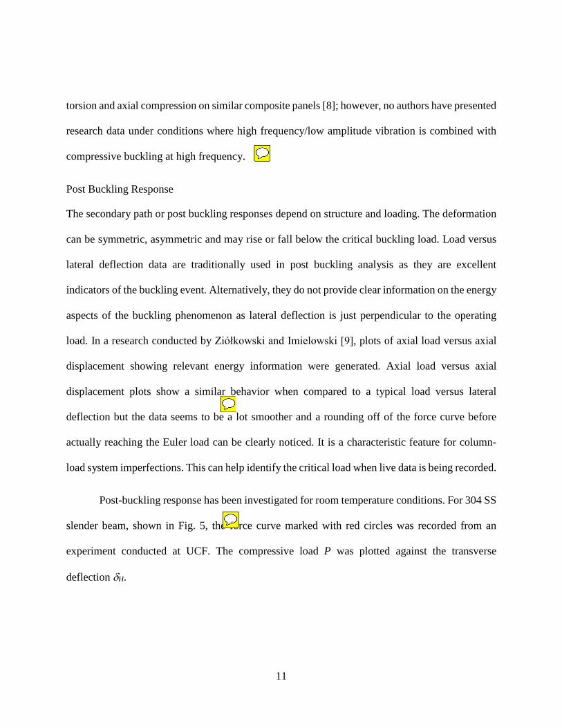
Post-buckling response has been investigated for room temperature conditions. For 304 SS
slender beam, shown in Fig. 5, the force curve marked with red circles was recorded from an
experiment conducted at UCF. The compressive load P was plotted against the transverse
deflection δH.
11
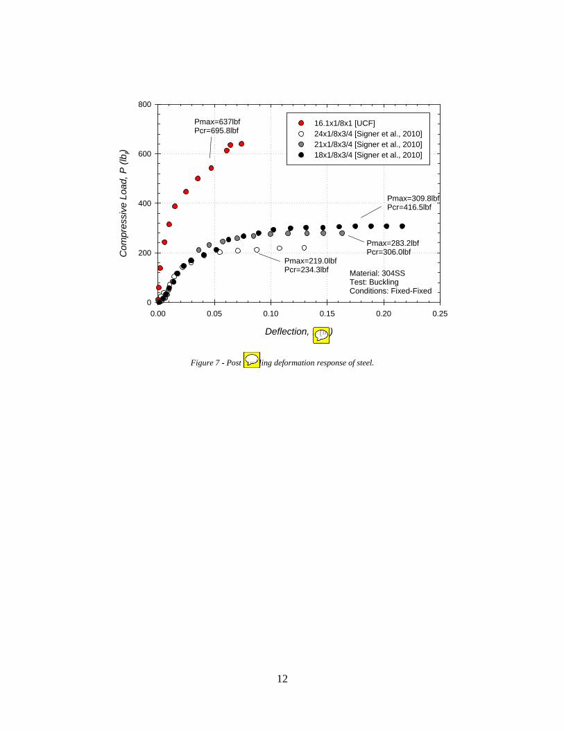
Figure 7 - Post buckling deformation response of steel.
Deflection, (in)
0.00 0.05 0.10 0.15 0.20 0.25
Com
pres
sive
Loa
d, P
(lb f)
0
200
400
600
800
16.1x1/8x1 [UCF] 24x1/8x3/4 [Signer et al., 2010] 21x1/8x3/4 [Signer et al., 2010] 18x1/8x3/4 [Signer et al., 2010]
Pmax=309.8lbfPcr=416.5lbf
Pmax=283.2lbfPcr=306.0lbf
Pmax=219.0lbfPcr=234.3lbf
Pmax=637lbfPcr=695.8lbf
Material: 304SSTest: BucklingConditions: Fixed-Fixed
12
Chapter 3. Experimental Approach
Test Requirements
Figure 8 – Bi-clamped testing condition of a 0.41m long specimen.
In order to predict critical bucking in the combined thermo-acousto-mechanical
environment, the device must be able to produce accurate buckling response of the specimen used.
For this, two sets of experiments will be conducted. The first set of experiments is intended to
calibrate and evaluate the performance of the main components of the device, the response of the
specimens will be investigated under mechanical cyclic loading (displacement/force control),
transverse vibration (250 to 500Hz, 120dB) and thermal cycles (RT to 0.5Tm) separately. For the
second set, the full buckling response of the specimens will be investigated and compared with
theoretical and simulated data. Lastly, the buckling response of the specimens will be investigated
under the combined thermo-acousto-mechanical cycles. The device should be able to provide data
for specimens allowed to be elastically deformed to determine the relationship between the
cumulative contributions of each load in the elastic deformation range and attempt to use this
13

information to predict the critical load. The loads will be plotted against the displacement history
of the midpoint of the specimen which can provide information about the nature of the deformation
and the fatigue life of the component. Models of the loads with respect to vertical displacement
will also be generated which can provide information on the energy aspects of the buckling
phenomenon. Further data analysis will be illustrated later on
Finally, the device will be ready to perform service like test profiles developed using
available data history to generate test data that will facilitate the development of mechanical
properties utilized in modeling and simulations of the fuselage components.
Test device Design
The developed test platform is composed of three sub-systems: a Sanderson universal manual
column buckling test frame, a customized quartz-lamp furnace and an acoustic horn.
Figure 9 Reconfiguration of the Sanderson frame
14

The Sanderson load frame has been reconfigured (Fig. 7) to allow automated cyclic
mechanical loads with the addition of a motor on the lever arm. A translation screw of 1.80 mm
per rotation is used to generate the motion of the lever arm. The load frame is equipped with a
washer-type load cell (Futek model: LTD 400) positioned at the upper fixed-end boundary of the
column specimen to help maintain desired load, a linear displacement transducer (Omega model:
LD621-15) on the left side of the load frame that measures the horizontal component of deflection
of the specimen, and a second transducer is mounted on the right end of the lever arm to allow the
computation of the vertical component of the specimen deflection. The load frame has the ability
to accommodate several specimen size from 0.40m to 0.8m, with a 0.05m increment and a
thickness of up to 0.004m.
Figure 10 Load Cell Calibration
The compressive load cell was subjected to a known loads between 0kN (0V) and 3.7kN
(2.1V). Known displacements between 0 (0V) and 15mm (10V) were prescribed to the spring-
loaded, displacement transducer. A high-torque servo-motor was used to drive the power-screw
connected to the lever arm. The vertical displacement transducer and the middle plane of the
specimen are exactly 0.53m and 0.15m away from the pivot point of the lever arm respectively.
0100200300400500600700800900
0 1 2 3
Com
pres
sive
Loa
d (lb
)
Volts
15

Using similar triangle relationships, the vertical displacement of the specimen is determined from
the reading of the vertical transducer. Additional power is supplied to both the load cell,
displacement transducer, and the motor via fixed DC power supplies. Input voltage was applied to
the motor, and the resulting angular velocity (in rad/s) was determined through a stroboscope. For
the motor, an H-bridge circuit combines the fixed power with oscillating signal from the chassis.
Figure 11 Furnace triangular design
The furnace houses up to a total of six 120V 2000W lamps, four of which are used to
provide a uniform heat distribution around the specimen. Behind the lamps, reflective material is
attached to the triangular furnace sections to increase the maximum heat potential of the system.
Triangular furnace sections were chosen to give a channel for the acoustic system (Fig. 9). The
heating elements are controlled by a LabView VI leading to a Watlow PID controller, which sends
a control current to a 208V 20A power supply (Research Inc. model: 5620-21-SP34) wired into
the four lamp circuit. Five thermocouples attach to the sample at 0%, 33%, 50%, 66%, and 100%
length L positions in order to get a temperature profile, and the thermocouple placed at 50% is
used for PID calculation. All five thermocouples route data back to LabView for recording. The
16

furnace is capable of reaching a maximum temperature of 400°C. For now, a cooling system has
not been integrated in the thermal control of the system but it can be integrated in future versions
of the device.
Figure 12 Thermocouple settings for temperature profile and PID control
Figure 13 Horn assembly on 8020 frame
The hardware for the acoustic system consists of two ICP accelerometers (Piezotronics
model: PCB 352B10), a power amplifier (Russound model: R290DS), a horn driver (BMS model:
4591), and a wave guide (SL Custom 250Hz Tractrix). The driver/horn assembly is mounted with
an 8020™ extruded aluminum frame. The frame is made adjustable so that is can be adjusted
accordingly to the length of any specimen. An oscillatory voltage waveform (sinusoidal or
17

triangular) of frequency, fa, of 250 or 500Hz and amplitude of 328mV, is output from the NI cDAQ
chassis to a 2-channel, dual-source power amplifier (Russound model: R290DS). An 8 or 16Ohm
signal is sent to a 2” mid-range, compression driver (BMS model: 4591). A flat front, tractrix-
curved waveguide is flush-mounted to the driver. Pre-calibrated (10mV/g), miniature
accelerometers (Piezotronics model: PCB 352B10) were attached to the tip of the waveguide and
along the length of the sample.
Figure 14 Accelerometers on sample
18
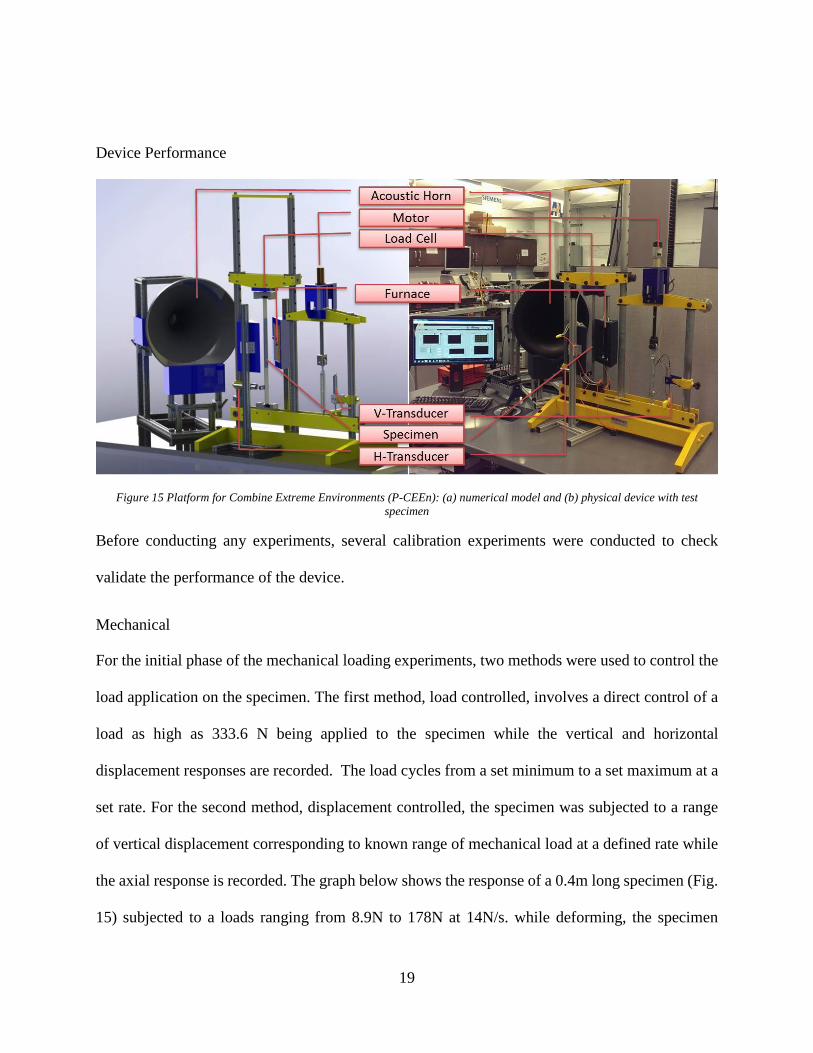
Device Performance
Figure 15 Platform for Combine Extreme Environments (P-CEEn): (a) numerical model and (b) physical device with test
specimen
Before conducting any experiments, several calibration experiments were conducted to check
validate the performance of the device.
Mechanical
For the initial phase of the mechanical loading experiments, two methods were used to control the
load application on the specimen. The first method, load controlled, involves a direct control of a
load as high as 333.6 N being applied to the specimen while the vertical and horizontal
displacement responses are recorded. The load cycles from a set minimum to a set maximum at a
set rate. For the second method, displacement controlled, the specimen was subjected to a range
of vertical displacement corresponding to known range of mechanical load at a defined rate while
the axial response is recorded. The graph below shows the response of a 0.4m long specimen (Fig.
15) subjected to a loads ranging from 8.9N to 178N at 14N/s. while deforming, the specimen
19

maintained a uniform sinusoidal shape. This data confirms the flexibility of the device when it
comes to performing load controlled or displacement controlled experiments.
Figure 16 Initial load- and displacement-controlled deformation response of specimen A2
Another important feature of the mechanical component of the device is to be able to apply
a mechanical cycling loads to a specimen and record it consistently. For this, a triangular waveform
signal was sent to the load control with a maximum load cycle P such that crP P . Load vs time
and load vs displacement were recorded and plotted below.
20

Figure 17 Cycle load Pmax=190N, Pcr=1014N, L=0.4572
The maximum applied load Pmax (190 N) is only 18.7% of the theoretical critical load (1014
N). The specimen is not expected to deform plastically and this is confirmed in the consistent load
vs δH response shown in Figure 17.
Figure 18 8 consecutive and consistent cycles
-5
0
5
10
15
20
25
30
35
40
45
0 50 100 150 200 250 300 350 400 450 500
Load
(N)
Time (s)
0
5
10
15
20
25
30
35
40
45
0 0.05 0.1 0.15
P (N
)
δH (mm)
21

Thermal
As stated earlier, the thermal component of the device is only composed of a heating element. The
furnace works perfect for isothermal experiments. When it comes to thermal cycling, due to the
lack of a cooling system the temperature rises accordingly but does not cool down very fast below
the 300°C range. The performance of the furnace is shown below.
Figure 19 Furnace performance
The data from Figure 19 shows that the temperature profile is not symmetric since the
thermocouple reading at the 66% is higher than the reading at 33% due to asymmetric heat flow
convection. The thermocouples at 0% and 100% were reading near room temperature.
Acoustical
Thus far, the equipment has performed well at 120dBSPL with both triangular and sinusoidal
waveforms, with exceptional performance at 500Hz. Figure 20 shows the acceleration experienced
22

(in gs) at the bottom and mid-point of a test-sample, as well as the acceleration experienced at the
mounting fringe of the horn
Figure 20 Acoustic transfer efficiency
Figure 21 Specimen used in the initial phase
-150
-100
-50
0
50
100
150
-0.7
-0.5
-0.3
-0.1
0.1
0.3
0.5
0.7
0 0.01 0.02 0.03 0.04
dBg
Horn [g] Sample (Bottom) [g]
Sample (50%) [g] Control Signal [dB]
23

Test Material
When comparing the elastic buckling behavior of a given structure and that of a geometrically
similar model structure not necessarily made of the same material, the Poisson’s ratio υ of the
materials is usually used as a reference for choice of material for buckling experiments [12]. It has
been proven that
2( / )crP EL C= (6)
Where C is a dimensionless number for all similar elastic structures, and
2( / ) ( )crP EL f υ= (7)
And therefore, for material with equal Poisson’s ratio,
2.1 2 1 2 1 2( / ) ( / )( / )cr crP P E E L L= (8)
Several samples of multipurpose 304 stainless steel, having identically uniform cross sections (i.e.,
a = 3.18mm by b = 25.4mm) but a range of lengths (i.e., between L = 0.4m and 0.8m), were utilized
in the test bed development. The specimens are tested in the unpolished condition, and they were
incised from hot rolled plate stock (per ASTM A276). At room temperature, elastic modulus, E, is
193GPa, yield strength corresponds, 0.2%YS, to 207MPa, and the coefficient of thermal
expansion,α is 5.3×10⁻⁶°C.
To evaluate the test device, three specimen sizes were chosen and they are described in the table
below. freeL represents the unclamped portion of the specimen which is the value used to calculate
the theoretical critical load using Euler’s equation.
24

Table 1 Specimen dimensions and properties
Specimen E (Gpa) LTotal(m) Lfree(m) a(m) b(m) I(m4) Pcr (kN) S 28 193 0.71 0.69 0.0254 0.00229 2.52861E-11 0.4092 S 30 193 0.76 0.74 0.0254 0.00229 2.52861E-11 0.3547 S 32 193 0.81 0.79 0.0254 0.00229 2.52861E-11 0.3104
Mechanical Model
The critical load crP of a specimen experimental is usually observed from a P vs δ curve.
That would require a complete buckling response of the specimen and potentially deform the
specimen plastically. The experiments intended to be performed on the specimens are restricted to
the elastic region of the material. Therefore an accurate method capable of predicting the critical
buckling of the specimen is needed.
Southwell’s method is a widely used technique that provides a graphical method for nondestructive
critical-load testing of columns as well as other structural components that may fail by buckling.
It has already been used by Fisher in a combined axial and transverse loading (a typical loading
for an airplane spar in test or flight. Southwell observed that for a lateral deflection Hδ under a
given load crP P< [13]
( )HH M k
Pδδ = − (9)
Where crM P= and k is a constant. Equation 9 is the equation of a straight line of slope crP . The
Southwell plot is illustrated below. Derivation can be found in [12], [14].
25

Figure 22 Southwell Plot
26

Chapter 4. Results
Mechanical
Combined
27

Chapter 5. Numerical Simulations
SOLIDWORKS is used to simulate the buckling experiment. Buckling analysis is tightly
integrated with SOLIDWORKS CAD and allows the calculation of critical failure loads of slender
structures under compression.
Figure 23 Software used for simulation
Specimen Model
First, a CAD model was generated for each specimen the exact dimension as shown below.
Figure 24 Specimen CAD and dimensions
28

The model was generated as close as possible to a real specimen. Surfaces were added at the
extremities of the model to replicate the contact surfaces between the specimen and the clamps of
the test device.
Finite Element Model
The next step in the finite element analysis was to set the boundary conditions. Two
features were used to apply the boundary conditions to the model. A fixed geometry restraint was
applied to the bottom of the specimen to set all the translational degrees of freedom to zero.
Figure 25 Fixed geometry feature
Then a Roller/Slider was applied to the top faces in contact with the clamps to only allow for
vertical motion of the top extremity of the sample as a force is being applied to it. The extremities
inside the Roller/Slider and fixed geometry constrains are not allowed to deflect or rotate (i.e.
(0) 0Hδ = , ( ) 0H Lδ = ).
29
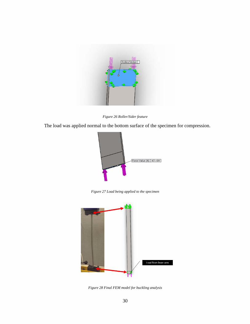
Figure 26 Roller/Sider feature
The load was applied normal to the bottom surface of the specimen for compression.
Figure 27 Load being applied to the specimen
Figure 28 Final FEM model for buckling analysis
30

Results
The graphs below show the results of the buckling analysis of the specimens where the critical
load and the maximum deformation are calculated. Those results are summarized in Table 2.
Figure 29 Buckling analysis of specimen S28
31

Figure 30 Buckling analysis of specimen S30
32

Figure 31 Buckling analysis of specimen S32
Table 2 Buckling analysis simulation
Specimen Pcr (kN) δH max(mm) S 28 0.4037 18.6 S 30 0.3502 20.7 S 32 0.3066 22.8
Chapter 6. Comparisons and Observations
Chapter 7. Conclusion
33

References
[1] Karasek M. L, Husehin Sehitoglu, and D. C. Slavik. "Deformation and Fatigue Damage in
1070 Steel Under Thermal Loading." Low Cycle Fatigue (1988): 184-205.
[2] Galambos, T. V. Guide to Stability Design Criteria for Metal Structures, 4th ed. New York:
John Wiley, 1988.
[3] Wang C. M., Wang C. Y., Reddy J. N. Exact Solution for Buckling of Structural Members.
Boca Raton: CRC Press LLC, 2005.
[4] Bazant, Zdenek P. Stability of Structures. New York: Oxford University Press, 1991.
[5] Hibbeler R., C. Mechanics Of Materials. Boston: Prentice Hall, 2011.
[6] Carpinteri A., Malvano R., Manuello A., Piana G. "Fundamental frequency evolution in
slender beams." Journal of Sound and Vibration (2014): 2390–2403.
[7] Weiyong Wang, Venkatesh Kodur, Xingcai Yang, Guoqiang Li. "Experimental study on
local buckling of axially compressed steel stub." Thin-Walled Structures (2014): 33–45.
[8] Abramovich, H. "Experimental Studies of Stiffened Composite Panels under Axial
Compression, Toorsion and Combined Loading." Falzon B G & Aliabadi H M,. Buckling
and Postbuckling Structures. London: Imperial College Press, 2008. 1-37.
[9] Ziółkowski A., Imiełowski S. "Buckling and Post-buckling Behavior of Prismatic Aluminum
Columns Submitted to a Series of Compressive Loads." Experimental Mechanics (2011):
1335–1345.
[10] Wang, Y. C., and Moore, D. B. "‘Effect of thermal restraint on column behaviour in a
frame." 4th Int. Symp. on Fire Safety Science, T. Kashiwagi (1994): 1055 – 106
34

[11] Archer, Robert R, and Thomas J Lardner. An Introduction to the Mechanics of Solids. New
York: McGraw-Hill, 1978. Print.
[12] Singer, J, Johann Arbocz, and T Weller. Buckling Experiments. Chichester: Wiley, 1998.
Print.
[13] Fisher, H. R. 'An Extension of Southwell's Method of Analyzing Experimental Observations
in Problems of Elastic Stability'. Proceedings of the Royal Society A: Mathematical,
Physical and Engineering Sciences 144.853 (1934): 609-630. Web.
[14] Hoff, Nicholas J. The Analysis Of Structures, Based On The Minimal Principles And The Principle Of
Virtual Displacements. New York: Wiley, 1956. Print.
35


