Decoupling Land Values in Residential Property Prices:
Smoothing Methods for Hedonic Imputed Price Indices
Alicia N. Rambaldi (University of Queensland, Australia)
Ryan R. J. McAllister (Commonwealth Scientific and Industrial Research Organisation, CSIRO)
Cameron S. Fletcher (Commonwealth Scientific and Industrial Research Organisation, CSIRO))
Paper prepared for the 34
th IARIW General Conference
Dresden, Germany, August 21-27, 2016
Session 6A: Accounting for Real Estate
Time: Thursday, August 25, 2016 [Afternoon]
Decoupling land values in residential property prices: smoothing methods for
hedonic imputed price indices
⇤
Alicia N. Rambaldi(1), Ryan R. J. McAllister(2), Cameron S. Fletcher(3)
(1)School of Economics, The University of Queensland, St Lucia, QLD 4072. Australia; (2) CSIRO, BoggoRoad, Dutton Park, Brisbane, QLD 4102. Australia; (3) CSIRO, PO Box 780, Atherton, QLD 4883.Australia
Abstract
A property is a bundled good composed of an appreciating asset, land, and a depre-ciating asset, structure. The motivation to separate the value of the land and structurecomponents of property prices includes a range of needs such as those of tax authorities,climate adaptation research, and national accounting. Recent approaches to disentan-gling these two assets have been based on employing non-linearities and a constructionprice index as an instrument. This study proposes to identify them by treating them astwo unobserved components of the property price, each with a unique mapping to intrin-sic hedonic characteristics and different dynamic behaviour. The estimation approachuses a modified form of the Kalman filter. One advantage of the model estimationstrategy is that the estimated components and derived indices are less influenced by thecomposition of sales at any given period even when the model is estimated at higherfrequencies (e.g. monthly instead of quarterly). The algorithm is simple to implementand we demonstrate, using three datasets representing different urban settings in twocountries, that the method produces land value predictions comparable to the state val-uer’s assessments, and price indices comparable to recently published alternatives thatrely on exogenous non-market information to disentangle land values. Our monthlyindices are smoother than the quarterly counterparts produced by alternative methods.
Keywords: urban land prices, housing prices, state-space, unobserved components,
Fisher price indices.
JEL: C53, C43, R31⇤The authors acknowledge funding from the Australian Research Council (DP120102124), the Australian
Government (Department of Climate Change and Energy Efficiency) and the National Climate ChangeAdaptation Research Facility.
1

1 Introduction
A property is a bundled good composed of an appreciating asset, land, and a depreciating
asset, structure. The importance of this distinction is increasingly recognized in both the
real estate (see Bostic et al. (2009), Malpezzi et al. (1987)) and the price index construction
literature (see European Comission et al. (2013), Chapter 13, Diewert et al. (2011, 2015) and
Diewert and Shimizu (2013)). The motivations to separate the value of the land and struc-
ture components of property prices include the needs of tax authorities, climate adaptation
research (Fletcher et al., 2013), and national accounting (Diewert et al., 2015). The literature
review of Diewert et al. (2015) concludes that land and structure should be modelled as two
additive components of the property value. This is the view we adopt as well.
Our paper provides an econometric approach to both obtaining the decomposition of the
price of a residential property into land and structure components, and computing price in-
dices for each component. The underlying economic model is a representation of the valuer’s
problem, whose task is to provide a valuation of either the property or the land. Economet-
rically, the identification makes use of the fact that each component (land/structure) can
be mapped to unique characteristics with behaviours that differ dynamically. The economic
arguments to justify the dynamic behaviour of each component are based on existing liter-
ature (see for example Bostic et al. (2009)). Due to the mobility of materials and labor,
construction costs are generally uniform within a housing market and thus it must be the
case that asymmetric appreciation across properties within a market arise from asymmetric
exposure to common shocks to land values. At any point in time the value of the structure is
its replacement cost less any accumulated depreciation. Thus, sufficiently large depreciation
can result in the structure (improvements on the land) declining in value over time1. Using
dynamic behaviour to separate unobserved components is an idea that dates back to Mar-
avall and Aigner (1977) and has been used recently in a number of contexts (e.g. separating1see Malpezzi et al. (1987) and Knight and Sirmans (1996) for an excellent discussion and treatment of
modeling and accounting for depreciation and maintenance of the structure
2

measurement error, Komumjer and Ng (2014), inflation and output gap, Harvey (2011)). Our
identification strategy is to use ’dynamic discount factors’, popular in the Bayesian statistics
literature dating back to the 1970s (see Koop and Korobilis (2013) for a recent application
in econometrics). We write the model in state-space form, specify part of the covariance
structure using discount factors and estimate in a classical framework. The estimation uses a
modified form of the Kalman filter algorithm. The parameters associated with the covariance
structure are estimated by evaluating the log-likelihood and those associated with the hedo-
nic characteristics by running the modified Kalman filter equations. The method proposed
here departs from recently proposed approaches to separate land and structure components,
Diewert et al. (2015) and Färe et al. (2015), in that we do not rely on the use of exogenous
price information as instruments to identify the components.
The use of hedonic characteristics that define the land and structure components is a fea-
ture of other recent works (structure size, distance to public transport, etc). In Diewert et al.
(2011), the focus is on non-linear hedonic regressions with specifications that use piecewise
or spline functions of the characteristics. However, the use of non-linearities is not sufficient
to separate the two components. In their most recent work, Diewert et al. (2015), the model
specification uses piecewise or spline functions of the characteristics together with exogenous
price information in the form of a construction price index which is used as instrument to
identify the land component (we refer to their approach as DdH). Diewert and Shimizu (2013)
use a similar approach to compute components price indices for Tokyo. Färe et al. (2015)
also use the construction price index as an instrument to develop further the DdH approach
(although they refer to it as the DS method after the work of Diewert and Shimizu (2013)).
Their estimator is based on a distance function approach; we will refer to their approach as
FGSS. Färe et al. (2015) estimates econometric models with fixed parameters over the whole
sample. This leads to index values that are functions of future market information. This is
not a desirable characteristic. DdH use a period by period estimation of the model to con-
struct the price indices, which might lead to excessive volatility due the varying composition
3

of sales of the available sample in each time period. Our estimate of each component at any
period, ⌧, is a weighted sum of information in periods t = 1, . . . , ⌧ � 1, ⌧ . We construct two
hedonic imputed Fisher price indices. They differ in the type of weighting used for trans-
actions. When the weights are value shares (i.e. the weight of an individual transaction is
the ratio of its sale price to the sum of prices of all properties sold in that time period) the
index is labelled Fisher Plutocratic (FP). The index obtained by using equal weighting of
each transaction is labelled Fisher Democratic (FD). The computed indices from DhH and
FGSS are also Fisher type.
We use three data sets to demonstrate and evaluate our proposed method as well as
compare its performance against benchmarks. Two datasets from Queensland, Australia are
used to illustrate the estimation algorithm with data at two different frequencies (monthly
and annual) and compare the value of the predicted land component to that made by the
state valuer’s office. The third dataset from a Dutch city has been used by Diewert et al.
(2015) and Färe et al. (2015) to construct indices of land and structure components and thus
it provides the opportunity to compare the constructed hedonic imputed price indices from
our method to theirs.
2 The Valuer’s Model
In most developed countries there is the need to have a valuation for tax purposes of either
the property or the land. In the empirical application used in this paper, data from two urban
areas from the state of Queensland (QLD) in Australia are used. The state government has a
statutory authority (the Valuer-General of QLD) which issues land valuations for all rateable
properties in the state. These are then used by the local government to set ’rates’ or the state
to set land taxes. The valuations are typically carried out by expert assessors who use market
sales reports and local knowledge to provide an estimate of the value of the property/land
4

within a given property market2. The valuer’s task is to provide the tax authorities and
the rate payers with a valuation of their property or land. We write a simple model for the
expected value of the property,
Et
(Vt
) = Et
(Lt
, St
|⌧
X
j=0
wt�j
[market sales: Property, Land]t�j
) (1)
where,
Vt
is the value of the property
Lt
is the land component of the value
St
is the structure component of the property value
wt
is a weight such that wt�1 > w
t�2 > wt�3 > ...
The model simply states that the valuer uses all available information up to the current
period on market trends, sales in similar locations, sales of similar dwellings, and sales of land
and properties, and that transactions in more recent periods are more heavily weighted than
those that have occurred further in the past. When land valuation is required, the value,
Lt
, has to be disentangled from Vt
. This task requires the use of additional information
that can assist in separating the trends in the value of each of the goods in this bundle
(i.e., land and structure) and the assumption that the evolution of these two trends can be
differentiated. This assumption is justified using the arguments made in the previous section;
for the structure, the value is given by its construction cost minus depreciation. Therefore,
the value of a given structure is likely to be mostly dominated by the trend in wages and
materials costs in the local market and the depreciation due to age. For the land, on the
other hand, appreciation in a given market is often related to the limited supply of urban
land which results in common shocks to land values. For instance, there could be influx2The state government’s website makes the following statement regarding valuations: "When determining
statutory land values, valuers from our department: examine trends and sales information for each land use
category (e.g. residential, commercial, industrial and rural); inspect vacant or lightly improved properties
that have recently been sold; consider the land’s present use and zoning under the relevant planning scheme;
take into account physical attributes and constraints on use of the land" (http://www.dnrm.qld.gov.au/property/valuations/about/considerations).
5

of population into an area which would assert an upward pressure on the price of land.
In addition, location plays a big role as urban areas grow and expand. For instance, new
infrastructure (transport, bridges, train lines, etc) can result in big changes in the demand for
urban land in certain locations. It is obvious that the identification of the land value can be
assisted by observations of sales of vacant land; however, in heavily urbanised areas, land sales
are unusual. Using construction costs to identify the value of the structure is an alternative;
however, such a value would be an approximation, which would require some adjustment for
depreciation due to age as well as other intrinsic characteristics of the structure if available.
In other words, the valuers adjust prices based on hedonic characteristics. In practice, valuers
perform hedonic adjustment based on experience and data and it is unlikely that an explicit
econometric model is used, although this is likely to be changing as relevant data become
more readily available in electronic form and more research on statistically sound prediction
models becomes available. To contribute to the latter, our aim in the next subsection is to
set up an econometric specification that models the valuer’s tasks of obtaining the required
decomposition. The approach is based on an estimator that is a weighted sum of past
information and has well defined statistical properties.
3 The Econometric Approach to the Decomposition and
Construction of Price Indices
The aim of a our decomposition approach is to have a general model specification so that
it works with most datasets and is simple enough to be easily implemented. In addition,
we wish to obtain estimates that will not be subjected to frequent revisions as new data
are gathered, because the components’ estimates are also the inputs to the construction of
separate price indices for land and structure. We start by writing the observed sale price as
a sum of three additive components. This follows previous studies (Bostic et al. (2009) and
Diewert et al. (2015)) where three additive components are defined, land (L), structure (S )
6
and noise.
yt
= Lt
+ St
+ ✏t
(2)
where,
yt
is a vector (Nt
⇥ 1) with the sale price of each property (or vacant land) sold in period
t. That is, in each t, Nt
properties in the sample are sold.
Lt
is a vector (Nt
⇥ 1) where each row is the value of the land component for the ith
property sold in period t
St
is a vector (Nt
⇥ 1) where each row is the value of the structure component for the ith
property sold in period t, and Sit
= 0 if the sale is for vacant land
✏t
⇠ N(0, Ht
)
In order to capture the trends in Lt
and St
, we must specify some form for these two
components. We define functions of each component’s unique hedonic characteristics and
some unknown parameters so that the resulting estimates capture the underlying smooth
trends in Lt
and St
.
Lt
= f(XL
t
,↵L
t
) (3)
St
= g(XS
t
,↵S
t
) (4)
where,
XL
t
is an Nt
⇥ kl
matrix of hedonic characteristics intrinsic to the land component, e.g.
size of the lot, location
XS
t
is an Nt
⇥ ks
matrix of hedonic characteristics intrinsic to the structure component,
e.g. age, size of the structure
↵c
t
are vectors of unknown parameters, c = L, S
7

A simple, but very flexible, form of f() and g() is to use a linear combination of charac-
teristics and time-varying parameters,
Lt
= XL
t
↵L
t
(5)
St
= XS
t
↵S
t
(6)
We propose to achieve identification by specifying the law of motion of ↵L
t
and ↵S
t
as
driven by uncorrelated components’ specific discount factors in the covariance structure.
↵L
t
= ↵L
t�1 + ⌘Lt
(7)
↵s
t
= ↵s
t�1 + ⌘st
where,
↵L
t
is a vector of time-varying parameters associated with land characteristics
↵S
t
is a vector of time-varying parameters associated with structure characteristics
⌘Lt
⇠ N(0, QL
t
)
⌘St
⇠ N(0, QS
t
)
E(⌘t
⌘0t
) = Qt
=
2
6
6
4
QL
t
0
0 QS
t
3
7
7
5
; with ⌘t
=
⌘Lt
⌘St
�0
↵t
=
↵L
t
↵S
t
�0t = 1, . . . , T
↵0 ⇠ N(a0, P0) is the initial condition.
We do not specify Qt
directly, instead we use what is known as a dynamic discounting
approach that models ↵t
and its mean square error matrix, Pt
, with a modified form of the
Kalman filter. The approach originates in the engineering and statistics literature. There
are alternative decompositions of property prices depending on the final objective. Property
prices are well known to have trends, while XS
t
and XL
t
are unlikely to be trending variables.
8

The conventional decomposition is into an overall price trend and a quality adjustment linear
combination of hedonic characteristics and parameters. This feature has been conventionally
captured through the use of time dummy variables as well as the use of stochastic trends (see
Rambaldi and Fletcher (2014) for a review). This conventional decomposition of the price is
well suited to predict the bundle (structure and land); however, it cannot provide information
on the differential movements in the prices of land and structure. The specification chosen
here implies the time-varying parameters provide a venue to capture the time evolution
of the marginal value of hedonic characteristics (e.g. the shadow price of land close to a
Central Business District might be trending upwards at a much faster rate than the market
valuation of an extra bathroom). The specification should be viewed as a device to obtain a
decomposition that can identify the trends in the two components of the price. To achieve
this, the hedonic characteristics used must be uniquely attached to one component, and this
could not be achieved by having an intercept or standalone trend component.
3.1 Estimation of Components’ Parameters
Writing (2) using expressions (5) and (6), and defining Zt
=
XL
t
XS
t
�
, the vector of
observed prices is linked to the characteristics of those properties sold at time t, and the
vector ↵t
=
↵L
t
↵S
t
�0,
yt
= Zt
↵t
+ ✏t
(8)
↵t
= ↵t�1 + ⌘
t
(9)
To estimate ↵t
in equations (8), we use a modified version of the Kalman filter which
allows identification of ↵c
t
, c = L, S through a restriction on the dynamic evolution of ↵t
.
To show how this is achieved, we present the standard form of the Kalman filter algorithm
and then show how it is modified when discount factors are used (West and Harrison (1999),
9

Ch. 6 provides a detailed introduction to the use of dynamic discount factors in a Bayesian
setting). Although the use of discount factors has been limited to applications in the Bayesian
literature, the limiting behaviour of the mean square error of the Kalman filter when using
discounting has been studied by Triantafyllopoulos (2007) who shows the covariance of at|t
converges to a finite non singular covariance matrix that does not depend on P0.
Denote the filter estimate of ↵t�1|t�1 by a
t�1|t�1. Given the assumptions about ✏t
, ⌘t
,↵0,
we can write its distribution at�1|t�1 ⇠ N(↵
t�1, Pt�1|t�1). Given the form of the transition
equations (9), the prediction and updating equations in the standard Kalman filter are given
by the expressions
yt|t�1 = Z
t
at�1|t�1 (10)
at|t = a
t�1|t�1 +Kt
⌫t
⌫t
= yt
� Zt
at|t�1
Kt
= Pt|t�1Z
0t
F�1t
Pt|t = P
t|t�1 �Kt
Ft
K 0t
Ft
= Zt
Pt|t�1Z
0t
+Ht
(11)
Pt|t�1 = P
t�1|t�1 +Qt
(12)
The distribution of the one-step ahead prediction of yt
is yt|t�1 ⇠ N(y
t|t�1,Ft
). To estimate
the covariances Qt
and Ht
in a classical estimation context, the log-likelihood function is
written in prediction error form using ⌫t
, the one-step ahead prediction error, and its variance-
covariance, Ft
, which are obtained from the above Kalman filter recursions. The mean square
error of at|t�1 (in this case a
t|t�1 = at�1|t�1) is associated with P
t|t�1, and that of at�1|t�1 is
Pt�1|t�1. However, P
t�1|t�1 is the mean square error of at|t�1 if there is no stochastic change in
the state vectors from period t�1 to period t (Qt
= 0). This is the global model (converging
10

state); however, locally the dynamics are better captured by Qt
6= 0. In our case these are the
dynamics that will allow us to extract the underlying trends in the components. The dynamic
discounting literature specifies Pt|t�1 as a discounted P
t�1|t�1 by a proportion. As our model
has two components, we specify the problem with two discount factors, each associated with
one of the components. We write equation (12) as follows
Pt|t�1 = diag
n⇣
��1L
Pt�1|t�1,[1:kL,1:kL]
⌘
,⇣
��1S
Pt�1|t�1,[(kL+1):(kL+kS),(kL+1):(kL+kS)]
⌘o
(13)
where Pt|t�1 is a partitioned diagonal matrix with sub-matrices P[a,b] corresponding to the
land and structure components. Each partition is a function of a discount factor, 0 < �L
, �S
1, and Pt�1|t�1 associated with the movements in the land or the structure components in
the model in period t � 1. It is easy to verify that the estimates of the state, at|t, for one
component are still functions of both the land and the structure characteristics, XL
t
and XS
t
,
since Ft
is a function of Zt
.
Using (13) and (12), it is easy to derive an explicit form of Qt
which is equal to zero if the
discount factors are equal to 1. The conventional approach was to set the discount factors
to a value, see West and Harrison (1999), usually in the range between 0.85 and 0.99 for
models with components such as trend, seasonal and cyclical. Recently Koop and Korobilis
(2013), in the context of large time-varying parameter vector autoregressive models, proposed
to estimate discount factors, which they refer to as forgetting factors, through a Bayesian
model averaging approach. Here we combine a grid search and an evaluation of the likelihood
function in an iterative procedure (the full algorithm is described in the next subsection).
Based on the arguments made in the literature, land and structure require different dis-
count factors that obey the following restriction: �L
< �S
< 1. Urban land destined for
residential housing is an appreciating scarce asset, and thus shocks in the market due to
changes in population trends as well as overall macroeconomic conditions are expected to
drive the trend in land prices. The trend in the value of the structure is expected to be in
line with movements in construction costs, which are likely to closely follow changes in wages
11
and more generally CPI, as well as a more homogeneous evolution across markets (such
as major urban cities within a state or country). Individual structures will be subjected to
depreciation which would be a function of the age of the structure. This point is important
as it provides a strong argument for the need to include a measure of the age of the structure
in XS
t
.
Denoting by at
the estimate of ↵t
and by Pt
the mean squared error matrix of at
, con-
ditional on all information up to period t, the Kalman filter is a form of nowcasting and
provides estimates such that at
is a weighted sum of current and past information,
at
=t
X
j=1
wj
(at|t)yj (14)
Explicit forms of the weights, wj
(at|t), have been derived by Koopman and Harvey (2003)
based on the recursions of the Kalman filter. This work, as well as that presented in Harvey
and Koopman (2000), show the relationship between implied weighting patterns obtained
using the recursions of the Kalman filter, as used in this study, and those obtained using
kernels in the non-parametric literature. The weights are functions of current and past
values of the one-step ahead prediction error ⌫t
= yt
� Zt
at|t�1 and its mean squared error
matrix, Ft
, which is a function of present and past values of Ht
and Pt|t�1 in our modified
filter. The type of pattern of wj
(at|t) is such that, at any point t, a
t
is a function of current
sales data and a decreasing function of past sale prices, with weight, wt
(at|t), determined by
current and past Xc
t
(c = L, S), discount factors and Ht
. Assuming XL
t
and XS
t
capture the
characteristics of the land (including location) and the structure, it is reasonable to specify
the distribution of the noise, ✏t
, as spherical. Therefore, Ht
= �2✏
INt with N
t
the number of
transactions in period t.
3.2 Estimation of covariance parameters
All parameters associated with the functions (5) and (6), are in the state vector; thus, once
values of �2✏
, �L
, and �S
are available, it is clear from the recursions of the Kalman filter
12
that the estimates of the state, ↵t
, and its mean square error matrix, Pt
, can be computed.
To estimate = [�2✏
, �L
, �S
] we combine a grid search and an evaluation of the likelihood
function in an iterative procedure. We first obtain an initial estimate of �2✏
by running a
conventional regression with intercept time dummies. The algorithm is as follows:
Estimation Algorithm:
Initial Estimates of , : For �2✏
we run least squares on a model with fixed time dummies
and all regressors, XS and XL, and compute �2✏
from the OLS residuals. Given this
estimate, we run the Kalman filter equations over a grid of pairs of values [�L
, �s
] and
compute the squared correlation between the actual price and the predicted price of
each property (constructed as the sum of the predicted land and structure components).
This is a general R2 measure. The pair of discount factors that provides the highest
generalised R2 is taken as the initial estimates, [�L
, �S
].
Maximum Likelihood estimate of �2✏
: Given [�L
, �S
], a Newton-Raphson algorithm is
used to find the value, �2✏
, that maximises the log-likelihood function, using �2✏
as
initial value.
Final Estimates of �L
and �s
: Given �2✏
, we run the Kalman filter equations over a grid of
pairs of values [�L
, �s
] again and compute the squared correlation between the actual
price and the predicted price of each property. The value pair that provides the highest
squared correlation are the final estimates �L
and �S
.
The final estimates �2✏
, �L
and �S
are used in the filtering equations (10-13) to obtain the
estimates of ↵S
t
and ↵L
t
which are used to compute predicted prices of the components for
each property and time period using equations (5 and 6) with ↵c
t
replaced by act|t, c = L, S.
If the dataset contains a reasonable number of transactions of land only sales, we compute
both an overall correlation between each sale and the model’s prediction, but also compute
the generalised R2 to assess the accuracy of the model’s predictions of sales of land only.
13

The set of discount factors found to give the maximum generalised R2 for land sales is used.
The algorithm, coded in Matlab, is fully automated and runs in seconds for the datasets
used in this study. The grid search for the discount factor pairs, �L
�S
, covers 19 possible
combinations in the ranges dL
= 0.7 � 0.95 and dS
= 0.8 � 0.99, and so that dL
< dS
to
reflect the underlying restriction, �L
< �S
< 1.
In Section 4.1 we present an empirical implementation of the modelling and estimation
using two datasets. These two datasets represent two different urban settings and two time-
series frequencies. The first is an expanding urban area (monthly observations), while the
second is an old and well established suburb very close to the city’s central business district
(annual observations).
3.3 Hedonic Imputed Price Indices
Diewert et al. (2015) construct Fisher type indices for the price of the land component. The
component is identified econometrically through the use of exogenous information in the form
of a construction price index produced by a statistical agency. Färe et al. (2015) construct
Fisher type indices for the land and the structure. Their identification of the land component
also uses the exogenous construction price index. To identify a construction price index, they
use their constructed land price index as the exogenous instrument.
We compute Fisher price indices for the land and structure components estimated by
our approach. Two alternative Fisher indices are computed by using a different weighting
scheme, they are labeled Fisher Plutocratic (FP) and Fisher Democratic (FD), respectively.
The plutocratic version uses weights that are functions of value shares, and it is defined as:
F P
(t�s),t =q
LP
(t�s),t PP
(t�s),t (15)
where Lp
t�s,t
and P p
t�s,t
are respectively the Laspeyres and Paasche index numbers,
For the land component the indices are given by
14

Lp
(t�s),t =NsP
h=1wh
(t�s)
✓
P
Lt (xL
(t�s))
P
L(t�s)
(xL(t�s)
)
◆
; P p
(t�s),t =
"
NtP
h=1wh
t
✓
P
L(t�s)
(xLt )
P
Lt (xL
t )
◆
#�1
where,
PL
(t�s)(xj
t
) for s � 0 is a prediction of the value of the land component of property h, sold
at time t with characteristics Xj
t
(j = Land, Structure) using a vector of shadow prices for
time period t� s and the value shares defined as in (16).
For time t, the weight of property h sold in that period, wh
t
, is given by:
wh
t
=P h
t
NtP
n=1P n
t
(16)
where,
P h
t
is the observed sale price of property/land h and Nt
is the number of sales in period
t. Similarly, using the prediction of the structure component of property h, P S
(t�s)(xj
t
) the
structure price index is computed.
The Fisher democratic version of the index, FD
(t�s),t , is computed by replacing the weights,
wh
t
(wh
t�s
), by N�1t
(N�1t�s
), where Nt
(Nt�s
) are the number of observations at time t(t� s). In
this case each transaction within a given time period is given an equal weight.
Section 4.2 presents monthly hedonic imputed Fisher indices using data from a Dutch
city. The dataset has been labelled "Town of A" in previous studies (European Comission
et al. (2013), Diewert et al. (2011, 2015) and Färe et al. (2015)). These are compared to the
quarterly price indices produced by DdH and FGSS.
4 Empirical Implementation
In this section our estimation approach, the land/structure decomposition, and the construc-
tion of price indices for the components are illustrated using our three datasets. Each set
provides an opportunity to evaluate our method against comparative benchmarks. The two
datasets from Queensland, Australia are used to show the workings of the estimation algo-
15

rithm with data at two different frequencies (monthly and annual), and compare the value of
the predicted land component to that made by the state valuer’s office. The discussion is in
Section 4.1. The third dataset is that used by Diewert et al. (2015) and Färe et al. (2015) and
thus it provides the opportunity to compare the constructed hedonic imputed price indices
from this method to theirs. The discussion is presented in Section 4.2.
4.1 The Decomposition into Land and Structure
In this section we illustrate the model estimation and decomposition with two datasets. The
Bay side data contains monthly observations from an urban area north of the city of Brisbane.
What is sometimes labelled as the "greater Brisbane area" has expanded rapidly as the South
East of the state of Queensland (SEQ) underwent a large influx of population in the last two
to three decades. These data are from Fletcher et al. (2011). The BrisSub dataset is for
a single suburb in the inner city of Brisbane. The suburb is within five km of the central
business district (CBD) and one of the oldest and most well established in the city. These
data are annual and have been sourced from Rambaldi et al. (2013). Descriptive statistics
for these datasets appear in Appendix A.
4.1.1 Monthly Data - Bay Side
The data area is composed of several urban centres surrounding the Bay which act as satellite
suburbs to Brisbane. A substantial proportion of the population travel into Brisbane every
day to reach their employment location. The market in the Brisbane and "greater Brisbane"
region went through a boom period between 2001 and 2005 and this is reflected in the
number of transactions per month for that period. The market was more stable between
2005 and 2008. Figure 1 (top panel) shows the number and type of transactions per month
over the sample period which covers 1991:5 to 2010:9 (233 months). There are transactions
of properties (land and structure) as well as land only. The 2008 global financial crisis is
noticeable in that the number of transactions drops to levels similar to the early 1990s and
16
remained volatile for the rest of the sample. It is widely accepted that the influx of population
into the region, together with a lag in the release of new urban land, drove land prices up
substantially. Figure 2 shows the median price of land sales. In this data set there are a total
of 13088 transactions, 9774 are of properties and the rest are land. The sale of land in this
area is due to urban sprawling in the area known as ’South East Queensland’ (SEQ). Having
observations of both types of transactions is unusual, and thus this data set provides a unique
opportunity to test the method. In addition, a large number of hedonic characteristics of the
structure and land are available for each transaction. The available data contain sale price,
land characteristics (size and location) and structure characteristics (size, age, number of
bedrooms and bathrooms), see Table 3 in Appendix A. In the notation of equations (5) and
(6), these characteristics fit into XL
t
or XS
t
. Land area, structure footprint and age entered
as a quadratic function to capture the wide range of the data3.
The estimates of the land and structure components, Lt
and St
, are converted to pro-
portions for presentation. These estimates are presented in Figure 1 (bottom panel), and
Table 1 presents the estimates of the discount factors and the overall noise variance (�2✏
) at
each step of the algorithm. We note that the initial estimate of �2✏
, which is obtained from
a time-dummy regression, is very large compared to the maximum likelihood estimate of the
time-varying components model. This is a good indication that the model has been able to
capture most of the dynamics of the land and structure components.
The left bottom panel in Figure 1 shows the land value as a proportion of the property
transaction sale value. The proportion was around 60% over the period 2002 - 2007. The
global financial crises downturn is visible, and the proportion due to land is estimated a bit
lower for the last part of the sample. Looking at Figure 1’s top panel, it is clear that sales
of land only dried up over the period of late 2007 and 2008, and the recovery was slow over
the 2009-2010 period.
Concentrating on the sales of properties (i.e. ignoring land only transactions, bottom3Plots of some of the coefficient estimates are available from the conference paper version, the rest are
available upon request
17

20 40 60 80 100 120 140 160 180 200 2200
20
40
60
80
100
120
140
160
180
200
months,1991:5−2010:9
Nu
mb
er
of
Tra
nsa
ctio
ns
Property Sales
Land Sales
20 40 60 80 100 120 140 160 180 200 2200
0.1
0.2
0.3
0.4
0.5
0.6
0.7
0.8
0.9
1
Months, 1990:5 − 2010:9
Pro
po
rtio
n
20 40 60 80 100 120 140 160 180 200 2200
0.1
0.2
0.3
0.4
0.5
0.6
0.7
0.8
0.9
1
Months, 1990:5 − 2010:9
Pro
port
ion
Figure 1: Bay side - Number of (monthly) Transactions (top); Median of Estimated Proportion of LandComponent - all sales used in the estimation (bottom left) and Vacant land sales ignored in the estimation(bottom right)
18

0 50 100 150 2000
0.5
1
1.5
2
2.5
3
3.5x 10
5
1991:5 − 2010:9
Month
ly M
edia
n L
and P
rice
Figure 2: Bay side -Median of (monthly) Observed Vacant Land Prices
right in Figure 1), indicates that the value of the land component for existing properties in
this area was around 45-50% over the 00’s decade and after the global financial crisis the
land component accounted for between 40% and 45%. This would seem reasonable for an
area that was expanding and where property would not be sold for the purpose of replacing
a single detached dwelling by townhouses or terraces, as is the case of the suburb in inner
Brisbane studied in the next section.
Table 1: Estimates of = �2✏
, �L
, �S
- Bayside Data�2✏
�L
�S
Highest Gen R2
LandHighest Gen R2
AllModel: Property and Land Sales (N = 13088)
Initial Estimates 2.61e+03 0.7a 0.95a 0.768b 0.866c
Final Estimates(MLE/Highest
Gen R2)
46.734 0.7a 0.95a 0.768b 0.866c
Model: Property Sales (N = 9774)Initial
OLS/Highest R23.07e+03 0.7 0.90 0.857
Final Estimates(MLE/Generalised
R2)
233.17 0.7 0.90 0.857
aChosen using Gen R2 from Land transactions; bthis value is equal for dL
, dS
= [0.7, 0.95]and [0.7, 0.99]; cthis value is for d
L
, dS
= [0.7, 0.90]
19
4.1.2 Annual Data - BrisSub
The suburb (neighbourhood) is in the inner city of Brisbane. The dataset covers 41 years
from 1970 to 20104 (descriptive statistics are presented in Table 4 in Appendix A); however,
the number of transactions is very small and dispersed over the time period covered compared
to the previous dataset. For this reason the estimation frequency is annual. Nevertheless,
our method performs quite well when asked to predict the proportion of the sale value due
to the land component. We provide the comparison of the model’s predictions of land values
to those made by the state valuer’s office in the year 2009.
There are very few transactions of land only (about 2% of transactions) and they appear
in the latter part of the sample (Figure 3 top panel). This is consistent with sales of blocks
that would have housed a single dwelling (smaller and with a backyard) which are then
developed into townhouses or terrace type structures as the area undergoes a process of infill
due to its location and the substantial growth of the city of Brisbane.
The estimates of the covariance discount factor parameters are similar to those obtained
for the Bay side data set with �L
= 0.7 and �S
= 0.9. This is expected as both sub-markets
are part of SEQ, which has experienced massive increases in the property prices, especially in
the early to middle part of the 00’s. Analysts and commentators agree the massive increase
is in land prices.
Figure 3 (bottom panel) shows the estimated land proportion of the property value. The
first few years are expectedly hard to estimate as the number of transactions is very small
(top panel). However, the components estimator seems to gain traction relatively quickly
and provide a very reasonable trend from period ten (1980) onwards. The bottom panel plot
is based on all transactions and the estimates would indicate the proportion of the value of
the properties in this suburb in the decade 2001-2010 has been at a median of 55% to 70%.
Table 2 shows the Valuer’s estimated land value for the year 2009 as a ratio to the property
sale price for those properties in our dataset sold in 2009. The model estimates that the land42010 data only covers the first half of the year
20

value was 67% (median) of the property sale value for that year. The valuer’s median for those
properties is 72%. The land valuation provided to the property owner by the state valuer’s is
based on a three year moving average. This is viewed as a way of decreasing volatility. Our
method is also weighted average of past values; however, the past information is not equally
weighted as in a simple moving average. One shortcoming of an equally weighting method
is that when the market takes a turn in either direction (e.g. the global financial crisis, the
Brisbane floods), the land valuations’ adjustment to these changes will be lagged. This was
observed by rate payers after the 2011 Brisbane flood episode.
21

5 10 15 20 25 30 35 400
50
100
150
200
250
years,1970 − 2010
Num
ber
of T
ransa
ctio
ns
Property Sales
Land Sales
5 10 15 20 25 30 35 400
0.1
0.2
0.3
0.4
0.5
0.6
0.7
0.8
0.9
1
years, 1970− 2010
Pro
po
rtio
n
Figure 3: Brisbane Inner City - Number of (annual) Transactions (top); Median of Estimated Proportionof Land Component (bottom)
22

Table 2: Comparison of Land Price Valuation. State Valuer vs. ModelMonthSold Valuer’s Estimated
Land Proportion ofthe actual sale
price
# Properties
Jan-09 0.721 13Feb-09 0.704 11Mar-09 0.762 16Apr-09 0.741 17May-09 0.746 16Jun-09 0.675 9Jul-09 0.738 11Aug-09 0.673 13Sep-09 0.734 14Oct-09 0.617 19Nov-09 0.683 12Dec-09 0.716 15
Valuer’s Median 2009 0.716 166Model (Median for 2009) 0.669 166
4.2 Price Indices for Land and Structure
In this section we construct price indices for land and structure using the "Town of A"
dataset kindly provided by W.E. Diewert (used in Diewert et al. (2015)). A shorter and
earlier version of this dataset was used by Färe et al. (2015). We clean the data following the
detailed code by Diewert. The original dataset had 3543 transactions, and 3487 were kept
after the cleaning process. Table 5 in Appendix Aprovides the descriptive statistics of the
working sample.
We label the indices FP and FD for Fisher plutocratic and Fisher democratic, respectively
(see Section 3.3). Throughout this section, we use a postfix "_L" to denote the index relating
to land (e.g. FP_L), and a postfix "_S" to denote structure (e.g FP_S). In this dataset land
area is the only characteristic describing land values; the structure is captured by dwelling
size, age, number of floors, number of floors2, number of rooms and number of rooms2. The
estimated discount factors for this dataset are �L
= 0.8 and �S
= 0.9. A plot of the estimated
23

land proportion is presented in Appendix B.
We compare our indices to those computed by Diewert et al. (2015) and Färe et al. (2015).
Diewert et al. (2015) compute Fisher indices imputed from hedonic models that are non-linear
in the parameters (the economic modelling framework is labelled the Builder’s Model). To
assist with the identification, exogenous information in the form of a construction price index,
NDOPI (New Dwelling Output Price Index, published by the Central Bureau of Statistics of
Netherlands), is used as an instrument to estimate the land component. A model that uses
linear splines on lotsize, but no other hedonic information, is used to compute the indices
labelled DdH_P3. By adding additional characteristics to the model, such as rooms, the
version labelled DdH_P4 is produced. These are computed for a quarterly frequency.
Färe et al. (2015) adopt the same approach to the modelling. They refer to this as the
DS approach, derived from the work in Diewert and Shimizu (2013). In their paper the
index DS2 uses piecewise linear functions of the characteristics together with the NDOPI as
exogenous information. This index should be close to DdH_P4, although they were using
a shorter and earlier version of the ’Town of A’ dataset. Färe et al. (2015)’s contribution is
to estimate the models using a distance function approach. Their models are estimated by
Corrected OLS and using a Stochastic Frontier approach (SFA). Färe et al. (2015) compute
Fisher indices from their SFA estimates (we label these FGSS_SFA ). The index computed
from their SFA approach is then used by Färe et al. (2015) as the exogenous land price index
to identify the structure component in what they label DS2. We label their "Diewert and
Shimizu (2013); Diewert et al. (2015)" derived indices as FGSS_DS2. Their indices are also
computed for a quarterly frequency.
Figure 4 presents plots (for land and structure) showing our indices (computed monthly)
as well. Tables 6 and 7 in Appendix C presents the data behind these plots. The appendix
tables also show computed Fisher price indices for the property (labelled FP_p and FD_p).
These are constructed by adding the land and structure predicted prices to obtain the prop-
erty’s price and then using it as the imputed price in the Fisher’s indices formulae. Finally a
24

median index constructed by computing the monthly median price of observed transactions
and setting Feb05 =1 is also presented for reference. The DdH and FGSS indices are based
on 2005:Q1=1. For the purpose of presentation the quarterly estimates have been aligned
with the central monthly indices (e.g. Q1 is aligned with February, Q2 is aligned with May,
Q3 is aligned with August and Q4 is aligned with November).
The DdH and FGSS_DS indices are estimated period by period which explains their more
volatile nature. The FGSS_SFA index is much less volatile as the underlying econometric
model is a fixed parameter model estimated with the data for the complete sample. The
problem with this approach to estimation is that in practice the transactions that occurred
in 2005, for example, had no information of the 2007 market; however, the model uses the
2007 information when estimating the parameters that will be then used to compute the
index. Our approach has time-varying parameters that update as new information becomes
available. The estimator is conditional on past and current information on the market and
therefore improves on DhH by using weighted past and current information, and on FGSS as
it does not use future information to estimate the parameters of the hedonic function. As a
result, our estimates are less volatile than DdH, but are able to pick up the turns in market
conditions due to the inherited learning nature of the Kalman filter estimator.
DdH did not compute a separate structure price index from the data, and thus DdH_P3
and DdH_P4 are identical to each other, and equal to NDOPI (their instrument). FGSS_DS2_S
is computed by estimating the Builder’s model with FGSS_DS2_L as the exogenous land
price index (that is, as the instrument to identify the structure). Our indices, FD_S and
FP_S, are based on the estimated structure component, St
, and thus no other exogenous
information has been used in their computation. Further evidence of the effectiveness of our
proposed approach is provided by the fact that our structure indices are very close to the
NDOPI (bottom panel Figure 4). Our index is not computed from construction costs of new
dwellings, instead it is using the sample information on the characteristics of the individual
dwellings and controlling for depreciation due to their age.
25

0.850
0.900
0.950
1.000
1.050
1.100
1.150
1.200
Land Price Indices. Feb05=1 / Q105=1
FD_L FP_L DdH_P3_L DdH_P4_L FGSS_DS2_L FGSS_SFA_L
0.850
0.900
0.950
1.000
1.050
1.100
1.150
1.200
Structure Price Indices. Feb05=1 / Q105=1
FD_S FP_S DdH_P3_S DdH_P4_S FGSS_DS2_S FGSS_SFA_S
Figure 4: Dutch "Town of A" - Comparison of Computed Monthly Indices to DdH and FGSSQuarterly Alternatives (Data in Tables 6 and 7 (Appendix C))
26

5 Conclusion
We have proposed a new approach to decoupling property prices into land and structure and
have applied it to three widely different datasets. The approach is generalisable, applicable
to most datasets and simple to implement. We show our approach uses only prior sales infor-
mation, and has the flexibility to deal with varying data frequency. We have demonstrated
that it produces predictions of the land component of property values that are comparable to
those provided by the state valuer’s office. The imputed price indices for the land component
we generate are smoother than those produced by alternative methods. Importantly, our
computed indices do not rely on exogenous non-market price information on construction
costs in order to identify the land component of the price.
Developing better approaches for decoupling property prices into land and structure is
both important, and increasingly feasible. Both fair land taxation and economically sensible
urban development projects need to be informed by an understanding of what proportion of
the asset base is an appreciating asset (i.e. land), and what proportion is a depreciating asset
(i.e. house structure). Issues like climate change are raising the profile and importance of
making sound adaptation decisions. At the same time, electronic data on housing character-
istics are becoming more readily available, making approaches such as ours more accessible
to regular valuation.
Our paper starts by providing a simple underlying economic model, labelled the valuer’s
problem, whose task is to provide a valuation of either the property or the land. We then
propose an econometric representation of the problem. The identification of land and struc-
ture as two components is achieved through the use of dynamic discounting factors in a
modified form of the Kalman filter. Using well established behavioural patterns in the prices
of urban land and construction costs, we can impose econometrically a different dynamic be-
27

haviour in each of these components. We adopt a classical approach to the estimation, which
entails running the Kalman filter to evaluate the log-likelihood of the unknown covariance
parameters. The outcome of our paper is a generalisable approach that we hope responds to
emerging needs and data availability.
Appendices
A Descriptive Statistics
Table 3: Descriptive Statistics Bay sideMin Max Mean Median St.Dev
Sale Price (in 1000) 15.50 1250.00 191.77 161.50 129.44Land Characteristics
Flood Plain Dummy 0.00 1.00 0.06 0.00 0.23Large Plot Dummy 0.00 1.00 0.09 0.00 0.28Land area (hectarea) 0.03 1.06 0.10 0.06 0.11dist_coast (Km) 0.02 5.78 1.39 1.38 0.93dist_waterway (Km) 0.01 0.86 0.27 0.25 0.16dist_OffenIndus (Km) 0.18 8.38 2.87 2.27 1.83dist_parks (Km) 0.01 0.98 0.13 0.11 0.11dist_busStop (Km) 0.02 4.35 0.47 0.22 0.80dist_Schools (Km) 0.01 6.55 0.65 0.32 1.09dist_Shops (Km) 0.01 4.80 0.53 0.40 0.49dist_BoatRamp (Km) 0.06 6.29 1.97 1.60 1.46dist_PubsClubs (Km) 0.01 5.34 1.44 1.24 0.93dist_Hospitals (Km) 0.01 13.26 3.20 2.26 2.71
Structure CharacteristicsStructure=1 0.00 1.00 0.75 1.00 0.43Age (years) 0.00 86.00 11.94 10.00 11.44Structure Footprint (hectare) 0.00 0.09 0.02 0.02 0.01Number of Bathrooms 0.00 4.00 1.06 1.00 0.78Number of Bedrooms 0.00 8.00 2.52 3.00 1.58Number of Parking Spaces 0.00 5.00 1.39 1.00 1.12Total number of Transactions 13088Number of Months 233 (1991:5 2010:9)
28

Table 4: Descriptive Statistics BrisSub DataMin Max Mean Median St.Dev
Sale Price (in 1000) 2.60 4710.00 305.22 215.00 269.48Land Characteristics
Flood Dummy 0.00 1.00 0.04 0.00 0.20Land area (hectareas) 0.02 0.22 0.06 0.06 0.02dist_waterway (Km) 0.01 1.62 0.57 0.53 0.38dist_river (Km) 0.95 4.77 2.97 3.04 0.87dist_industry (Km) 0.00 2.62 1.00 0.91 0.66dist_park (Km) 0.01 0.56 0.18 0.16 0.12dist_bikeway (Km) 0.01 1.51 0.57 0.56 0.35dist_busstop (Km) 0.01 0.50 0.20 0.18 0.11dist_TrainStn (Km) 0.01 3.17 1.38 1.40 0.82dist_school (Km) 0.04 1.23 0.47 0.45 0.24dist_shops (Km) 0.00 1.09 0.36 0.33 0.19dist_CBD (Km) 2.46 5.77 3.97 3.97 0.82
Structure CharacteristicsPre-War 0.00 1.00 0.49 0.00 0.50War/Post War 0.00 1.00 0.37 0.00 0.48Late 20th C 0.00 1.00 0.07 0.00 0.26Contemporaneous 0.00 1.00 0.04 0.00 0.20Structure=1 0.00 1.00 0.98 1.00 0.15Structure footprint 0.00 0.10 0.02 0.02 0.01Number of Levels 0.00 4.00 1.10 1.00 0.36Number of Bathrooms 0.00 6.00 1.37 1.00 0.67Number of Bedrooms 0.00 8.00 3.04 3.00 0.91Number of Parking Spaces 0.00 8.00 1.66 2.00 0.78Total number of Transactions 3944Number of Years 41 (1970 2010)
29

Table 5: Town of A Descriptive Statisticsmin max mean median stdev
price (000Euros)
70 550 182.260 160 71.316
Land Characteristicsland (sq mts) 70 1344 258.060 217 152.310
Structure Characteristicshouse (sq mts) 65 352 126.560 120 29.841Age (years) 0 4 1.895 2 1.231
floors 1 6 2.878 3 0.478rooms 2 10 4.730 5 0.874
Number ofTransactions
3487
Number ofmonths
66 (2003:1 2008:6)
The data were cleaned following Diewert et al (2015). See footnotes 11,12,13.
We are indebted to W.E. Diewert for providing the data and cleaning code
B Land Component Proportion of the Price (monthly) -
Dutch "Town of A"
months,2003:1-2008:610 20 30 40 50 60
Pro
po
rtio
n
0
0.1
0.2
0.3
0.4
0.5
0.6
0.7
0.8
0.9
1
30

C Price Indices for the Town of A
Table 6: "Town of A" Land Price Indices
Month FD_p FP_p Median_I FP FD Quarter DdH P3 DdH P4 FGSS DS2 FGSS SFA
Aug-03 0.932 0.923 0.927 0.910 0.910 03:Q3 0.826 0.837
Sep-03 0.942 0.930 1.096 0.902 0.902
Oct-03 0.954 0.943 0.937 0.925 0.925
Nov-03 0.979 0.970 0.904 0.969 0.969 03:Q4 0.869 0.879
Dec-03 0.979 0.972 0.955 0.971 0.971
Jan-04 0.981 0.975 1.013 0.979 0.979
Feb-04 1.002 0.997 0.997 1.012 1.012 04:Q1 0.956 0.961
Mar-04 1.007 1.003 0.915 1.023 1.023
Apr-04 1.002 0.999 1.125 1.017 1.017
May-04 0.996 0.993 1.046 0.998 0.998 04:Q2 1.007 1.009
Jun-04 1.008 1.006 0.977 1.019 1.019
Jul-04 1.014 1.012 0.952 1.031 1.031
Aug-04 1.006 1.005 0.924 1.021 1.021 04:Q3 1.019 1.020
Sep-04 1.014 1.014 1.043 1.038 1.038
Oct-04 1.011 1.012 0.963 1.038 1.038
Nov-04 0.995 0.997 0.963 1.010 1.010 04:Q4 0.925 0.938
Dec-04 0.998 1.000 0.993 1.013 1.013
Jan-05 0.988 0.988 0.940 0.983 0.983
Feb-05 1.000 1.000 1.000 1.000 1.000 05:Q1 1.000 1.000 1.000 1.000
Mar-05 1.001 1.002 1.080 1.004 1.004
Apr-05 1.005 1.004 1.030 1.005 1.005
May-05 1.021 1.021 1.110 1.035 1.035 05:Q2 1.131 1.123 1.128 1.048
Jun-05 1.043 1.042 1.120 1.072 1.072
31
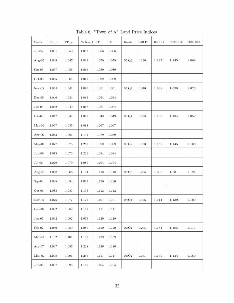
Table 6: "Town of A" Land Price Indices
Month FD_p FP_p Median_I FP FD Quarter DdH P3 DdH P4 FGSS DS2 FGSS SFA
Jul-05 1.051 1.050 1.080 1.086 1.086
Aug-05 1.048 1.047 1.023 1.079 1.079 05:Q3 1.136 1.127 1.145 1.068
Sep-05 1.057 1.056 1.066 1.089 1.089
Oct-05 1.065 1.064 1.017 1.099 1.099
Nov-05 1.044 1.041 1.096 1.051 1.051 05:Q4 1.040 1.038 1.030 1.023
Dec-05 1.046 1.044 1.063 1.054 1.054
Jan-06 1.052 1.049 1.068 1.064 1.064
Feb-06 1.047 1.044 1.096 1.049 1.049 06:Q1 1.108 1.109 1.134 1.052
Mar-06 1.057 1.055 1.088 1.067 1.067
Apr-06 1.063 1.061 1.142 1.079 1.079
May-06 1.077 1.075 1.256 1.099 1.099 06:Q2 1.170 1.159 1.145 1.100
Jun-06 1.075 1.073 1.206 1.094 1.094
Jul-06 1.079 1.079 1.080 1.104 1.104
Aug-06 1.088 1.088 1.194 1.118 1.118 06:Q3 1.225 1.208 1.231 1.124
Sep-06 1.095 1.094 1.063 1.130 1.130
Oct-06 1.083 1.083 1.133 1.112 1.112
Nov-06 1.076 1.077 1.129 1.101 1.101 06:Q4 1.126 1.114 1.139 1.100
Dec-06 1.082 1.082 1.198 1.111 1.111
Jan-07 1.092 1.092 1.075 1.129 1.129
Feb-07 1.089 1.089 1.080 1.120 1.120 07:Q1 1.205 1.184 1.185 1.177
Mar-07 1.102 1.101 1.136 1.139 1.139
Apr-07 1.097 1.096 1.228 1.126 1.126
May-07 1.098 1.096 1.256 1.117 1.117 07:Q2 1.161 1.139 1.134 1.160
Jun-07 1.097 1.095 1.156 1.104 1.104
32

Table 6: "Town of A" Land Price Indices
Month FD_p FP_p Median_I FP FD Quarter DdH P3 DdH P4 FGSS DS2 FGSS SFA
Jul-07 1.103 1.101 1.027 1.117 1.117
Aug-07 1.109 1.106 1.043 1.122 1.122 07:Q3 1.167 1.153 1.208 1.163
Sep-07 1.117 1.116 1.238 1.149 1.149
Oct-07 1.118 1.119 1.118 1.163 1.163
Nov-07 1.103 1.102 1.158 1.127 1.127 07:Q4 1.099 1.095 1.124 1.168
Dec-07 1.112 1.112 1.163 1.142 1.142
Jan-08 1.117 1.117 1.151 1.150 1.150
Feb-08 1.111 1.110 1.163 1.134 1.134 08:Q1 1.046 1.041 1.002 1.153
Mar-08 1.091 1.089 1.196 1.088 1.088
Apr-08 1.102 1.100 1.093 1.112 1.112
May-08 1.105 1.103 1.147 1.120 1.120 08:Q2 1.092 1.092 1.136 1.172
Jun-08 1.118 1.117 1.179 1.146 1.146
FD_p: Fisher Democratic (property); FD_l: Fisher Democratic (land);
FP_p: Fisher Plutocratic (property); FP_l: Fisher Plutocratic (land);
DdH_P3, DdH_P4: Land Price Indices; Diewert et al. (2015). Tables 1 and 2
FGSS_DS2, FGSS_SFA: Land Price Indices; DS and SFA computed by Färe et al. (2015) Table 5
33

Table 7: "Town of A" Structure Price Indices
Month FD_p FP_p Median_I FP FD Quarter DdH P3 DdH P4 FGSS DS2 FGSS SFA
Aug-03 0.932 0.923 0.927 0.946 0.931 03:Q3 1.016 1.016
Sep-03 0.942 0.930 1.096 0.966 0.946
Oct-03 0.954 0.943 0.937 0.972 0.953
Nov-03 0.979 0.970 0.904 0.985 0.970 03:Q4 1.008 1.008
Dec-03 0.979 0.972 0.955 0.985 0.972
Jan-04 0.981 0.975 1.013 0.984 0.972
Feb-04 1.002 0.997 0.997 0.996 0.988 04:Q1 1.000 1.000
Mar-04 1.007 1.003 0.915 0.998 0.990
Apr-04 1.002 0.999 1.125 0.994 0.989
May-04 0.996 0.993 1.046 0.995 0.989 04:Q2 0.975 0.975
Jun-04 1.008 1.006 0.977 1.002 0.998
Jul-04 1.014 1.012 0.952 1.004 1.000
Aug-04 1.006 1.005 0.924 0.998 0.995 04:Q3 0.984 0.984
Sep-04 1.014 1.014 1.043 1.000 1.000
Oct-04 1.011 1.012 0.963 0.995 0.996
Nov-04 0.995 0.997 0.963 0.986 0.989 04:Q4 1.016 1.016
Dec-04 0.998 1.000 0.993 0.989 0.991
Jan-05 0.988 0.988 0.940 0.991 0.992
Feb-05 1.000 1.000 1.000 1.000 1.000 05:Q1 1.000 1.000 1.000 1.000
Mar-05 1.001 1.002 1.080 0.999 0.999
Apr-05 1.005 1.004 1.030 1.005 1.004
May-05 1.021 1.021 1.110 1.014 1.012 05:Q2 0.993 0.993 1.039 1.041
Jun-05 1.043 1.042 1.120 1.028 1.025
Jul-05 1.051 1.050 1.080 1.033 1.030
34

Table 7: "Town of A" Structure Price Indices
Month FD_p FP_p Median_I FP FD Quarter DdH P3 DdH P4 FGSS DS2 FGSS SFA
Aug-05 1.048 1.047 1.023 1.031 1.028 05:Q3 1.015 1.015 1.070 1.090
Sep-05 1.057 1.056 1.066 1.039 1.038
Oct-05 1.065 1.064 1.017 1.047 1.043
Nov-05 1.044 1.041 1.096 1.040 1.035 05:Q4 1.039 1.045 1.050 1.054
Dec-05 1.046 1.044 1.063 1.043 1.038
Jan-06 1.052 1.049 1.068 1.046 1.041
Feb-06 1.047 1.044 1.096 1.048 1.043 06:Q1 1.007 1.007 1.061 1.062
Mar-06 1.057 1.055 1.088 1.054 1.048
Apr-06 1.063 1.061 1.142 1.057 1.051
May-06 1.077 1.075 1.256 1.067 1.061 06:Q2 1.017 1.017 1.055 1.053
Jun-06 1.075 1.073 1.206 1.064 1.061
Jul-06 1.079 1.079 1.080 1.065 1.063
Aug-06 1.088 1.088 1.194 1.071 1.070 06:Q3 1.012 1.012 1.082 1.087
Sep-06 1.095 1.094 1.063 1.074 1.073
Oct-06 1.083 1.083 1.133 1.065 1.065
Nov-06 1.076 1.077 1.129 1.061 1.060 06:Q4 1.015 1.015 1.048 1.073
Dec-06 1.082 1.082 1.198 1.062 1.063
Jan-07 1.092 1.092 1.075 1.068 1.068
Feb-07 1.089 1.089 1.080 1.070 1.069 07:Q1 1.034 1.034 1.029 1.084
Mar-07 1.102 1.101 1.136 1.081 1.078
Apr-07 1.097 1.096 1.228 1.078 1.075
May-07 1.098 1.096 1.256 1.085 1.081 07:Q2 1.045 1.045 1.056 1.127
Jun-07 1.097 1.095 1.156 1.091 1.086
Jul-07 1.103 1.101 1.027 1.093 1.089
35
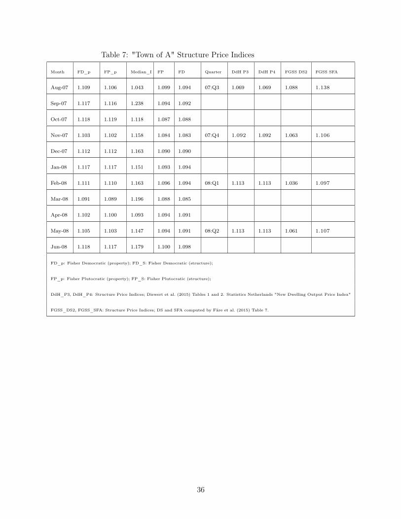
Table 7: "Town of A" Structure Price Indices
Month FD_p FP_p Median_I FP FD Quarter DdH P3 DdH P4 FGSS DS2 FGSS SFA
Aug-07 1.109 1.106 1.043 1.099 1.094 07:Q3 1.069 1.069 1.088 1.138
Sep-07 1.117 1.116 1.238 1.094 1.092
Oct-07 1.118 1.119 1.118 1.087 1.088
Nov-07 1.103 1.102 1.158 1.084 1.083 07:Q4 1.092 1.092 1.063 1.106
Dec-07 1.112 1.112 1.163 1.090 1.090
Jan-08 1.117 1.117 1.151 1.093 1.094
Feb-08 1.111 1.110 1.163 1.096 1.094 08:Q1 1.113 1.113 1.036 1.097
Mar-08 1.091 1.089 1.196 1.088 1.085
Apr-08 1.102 1.100 1.093 1.094 1.091
May-08 1.105 1.103 1.147 1.094 1.091 08:Q2 1.113 1.113 1.061 1.107
Jun-08 1.118 1.117 1.179 1.100 1.098
FD_p: Fisher Democratic (property); FD_S: Fisher Democratic (structure);
FP_p: Fisher Plutocratic (property); FP_S: Fisher Plutocratic (structure);
DdH_P3, DdH_P4: Structure Price Indices; Diewert et al. (2015) Tables 1 and 2. Statistics Netherlands "New Dwelling Output Price Index"
FGSS_DS2, FGSS_SFA: Structure Price Indices; DS and SFA computed by Färe et al. (2015) Table 7.
36
References
Bostic, R., Longhofer, S. D., and Redfearn, C. L. (2009). Land leverage: Decomposing home
price dynamics. Real Estate Economics, 35(2):183—208.
Diewert, W., de Haan, J., and Hendriks, R. (2011). The decomposition of a house price
index into land and structures components: A hedonic regression approach. The Valuation
Journal, 6:58–106.
Diewert, W. E., de Haan, J., and Hendriks, R. (2015). Hedonic regressions and the decompo-
sition of a house price index into land and structures components. Econometric Reviews,
34(1–2):106–126.
Diewert, W. E. and Shimizu, C. (2013). Residential property price indexes for tokyo. In
Real Estate Markets, Financial Crisis, and Economic Growth : An Integrated Economic
Approach. Working Paper No 3. Institute of Economic Research, Hitotsubashi University.
European Comission, Eurostat, OECD, and World Bank (2013). Handbook on Residential
Property Price indices (RPPIs). EUROSTAT. Bert Balk project coordinator, 2013 edition.
Färe, R., Grosskopf, S., Shang, C., and Sickles, R. (2015). Pricing characteristics: An
application of shephard’s dual lemma. manuscript.
Fletcher, C., Taylor, B., Rambaldi, A., Harman, B., Heyenga, S., Ganegodage, K., Lipkin,
F., and McAllister, R. (2013). Costs and coasts: an empirical assessment of physical
and institutional climate adaptation pathways. Number 37/13. National Climate Change
Adaptation Research Facility, Gold Coast.
Fletcher, C. S., McAllister, R. R. J., Rambaldi, A. N., and Collins, K. (2011). The economics
of adaptation to protect appreciating assets from coastal inundation. Final Report F110609,
CSIRO Climate Adaptation Flagship.
37

Harvey, A. C. (2011). Modelling the phillips curve with unobserved components. Applied
financial economics, 21:7–17.
Harvey, A. C. and Koopman, S. J. (2000). Signal extraction and the formulation of unobserved
components models. Econometrics Journal, 3:84–107.
Knight, J. and Sirmans, C. (1996). Depreciation, maintenance, and housing prices. Journal
of Housing Economics, 5:369—389.
Komumjer, I. and Ng, S. (2014). Measurement errors in dynamic models. Econometric
Theory.
Koop, G. and Korobilis, D. (2013). Large time-varying parameter {VARs}. Journal of
Econometrics, 177(2):185 – 198.
Koopman, S. and Harvey, A. (2003). Computing observation weights for signal extraction
and filtering. Journal of Economic Dynamics and Control, 27:1317–1333.
Malpezzi, S., Ozanne, L., and Thibodeau, T. (1987). Microeconomic estimates of housing
depreciation. Land Economics, 6:372—385.
Maravall, A. and Aigner, D. J. (1977). Latent Variables in Socio-economic models, chapter
Identification of the dynamic shock-error model: The case of dynamic regression. North-
Holland Pub. Co.,.
Rambaldi, A. N. and Fletcher, C. (2014). Hedonic imputed property price indexes: The
effects of econometric modeling choices. The Review of Income and Wealth, 60(777):758–.
Rambaldi, A. N., Fletcher, C., Collins, K., and McAllister, R. R. J. (2013). Housing shadow
prices in an inundation prone suburb. Urban Studies, 50(9):1889–1905.
Triantafyllopoulos, K. (2007). Convergence of discount time series dynamic linear models.
Communications in Statistics-Theory and Methods, 36(11):2117–2127.
38

West, M. and Harrison, J. (1999). Bayesian Forecasting and Dynamic Models. Springer
Berlin / Heidelberg.
39


