
1
Data Communications & Networks
Session 3 – Main Theme
Data Encoding and Transmission
Dr. Jean-Claude Franchitti
New York University
Computer Science Department
Courant Institute of Mathematical Sciences
Adapted from course textbook resources
Computer Networking: A Top-Down Approach, 6/E
Copyright 1996-2013
J.F. Kurose and K.W. Ross, All Rights Reserved

2
2 Data Encoding and Transmission
Agenda
1 Session Overview
3 Summary and Conclusion

3
What is the class about?
Course description and syllabus:
»http://www.nyu.edu/classes/jcf/csci-ga.2262-001/
»http://cs.nyu.edu/courses/fall14/CSCI-GA.2262-
001/index.html
Textbooks: » Computer Networking: A Top-Down Approach (6th Edition)
James F. Kurose, Keith W. Ross
Addison Wesley
ISBN-10: 0132856204, ISBN-13: 978-0132856201, 6th Edition (02/24/12)

4
Course Overview
Computer Networks and the Internet
Application Layer
Fundamental Data Structures: queues, ring buffers, finite state machines
Data Encoding and Transmission
Local Area Networks and Data Link Control
Wireless Communications
Packet Switching
OSI and Internet Protocol Architecture
Congestion Control and Flow Control Methods
Internet Protocols (IP, ARP, UDP, TCP)
Network (packet) Routing Algorithms (OSPF, Distance Vector)
IP Multicast
Sockets
5
Course Approach
Introduction to Basic Networking Concepts (Network Stack)
Origins of Naming, Addressing, and Routing (TCP, IP, DNS)
Physical Communication Layer
MAC Layer (Ethernet, Bridging)
Routing Protocols (Link State, Distance Vector)
Internet Routing (BGP, OSPF, Programmable Routers)
TCP Basics (Reliable/Unreliable)
Congestion Control
QoS, Fair Queuing, and Queuing Theory
Network Services – Multicast and Unicast
Extensions to Internet Architecture (NATs, IPv6, Proxies)
Network Hardware and Software (How to Build Networks, Routers)
Overlay Networks and Services (How to Implement Network Services)
Network Firewalls, Network Security, and Enterprise Networks

6
Data Transmission and Encoding Concepts
ADTs and Protocol Design
Summary and Conclusion
Data Transmission and Encoding Session in Brief

7
Icons / Metaphors
7
Common Realization
Information
Knowledge/Competency Pattern
Governance
Alignment
Solution Approach

8
2 Data Encoding and Transmission
Agenda
1 Session Overview
3 Summary and Conclusion

9
ADTs and Protocol Design
Data Encoding and Transmission - Roadmap
Data Encoding and Transmission Concepts
2 Data Encoding and Transmission

10
Simplified Data Communications Model

11
S(t) = A sin(2ft + Φ)

12
Terminology (1/3)
Transmitter
Receiver
Medium
Guided medium
E.g., twisted pair, optical fiber
Unguided medium
E.g., air, water, vacuum
13
Terminology (2/3)
Direct link
No intermediate devices
Point-to-point
Direct link
Only 2 devices share link
Multi-point
More than two devices share the link

14
Terminology (3/3)
Simplex
One direction
e.g., television
Half duplex
Either direction, but only one way at a time
e.g. police radio
Flux duplex
Both directions at the same time
e.g., telephone

15
Analog and Digital Data Transmission
Data
Entities that convey meaning
Signals
Electric or electromagnetic representations of
data
Transmission
Communication of data by propagation and
processing of signals

16
Data
Analog
Continuous values within some interval
e.g., sound, video
Digital
Discrete values
e.g., text, integers

17
Signals
Means by which data are propagated
Analog
Continuously variable
Various media
e.g., wire, fiber optic, space
Speech bandwidth 100Hz to 7kHz
Telephone bandwidth 300Hz to 3400Hz
Video bandwidth 4MHz
Digital
Use two DC components

18
Data and Signals
Usually use digital signals for digital data and
analog signals for analog data
Can use analog signal to carry digital data
Modem
Can use digital signal to carry analog data
Compact Disc audio

19
Analog Transmission
Analog signal transmitted without regard to
content
May be analog or digital data
Attenuated over distance
Use amplifiers to boost signal
Also amplifies noise
20
Digital Transmission
Concerned with content
Integrity endangered by noise, attenuation etc.
Repeaters used
Repeater receives signal
Extracts bit pattern
Retransmits
Attenuation is overcome
Noise is not amplified

21
Advantages/Disadvantages of Digital
Cheaper
Less susceptible to noise
Greater attenuation
Pulses become rounded and smaller
Leads to loss of information

22
Attenuation of Digital Signals

23
Interpreting Signals
Need to know
Timing of bits - when they start and end
Signal levels
Factors affecting successful interpreting of
signals
Signal to noise ratio
Data rate
Bandwidth

24
Encoding Schemes
Non-return to Zero-Level (NRZ-L)
Non-return to Zero Inverted (NRZI)
Bipolar –AMI
Pseudoternary
Manchester
Differential Manchester
B8ZS
HDB3

25
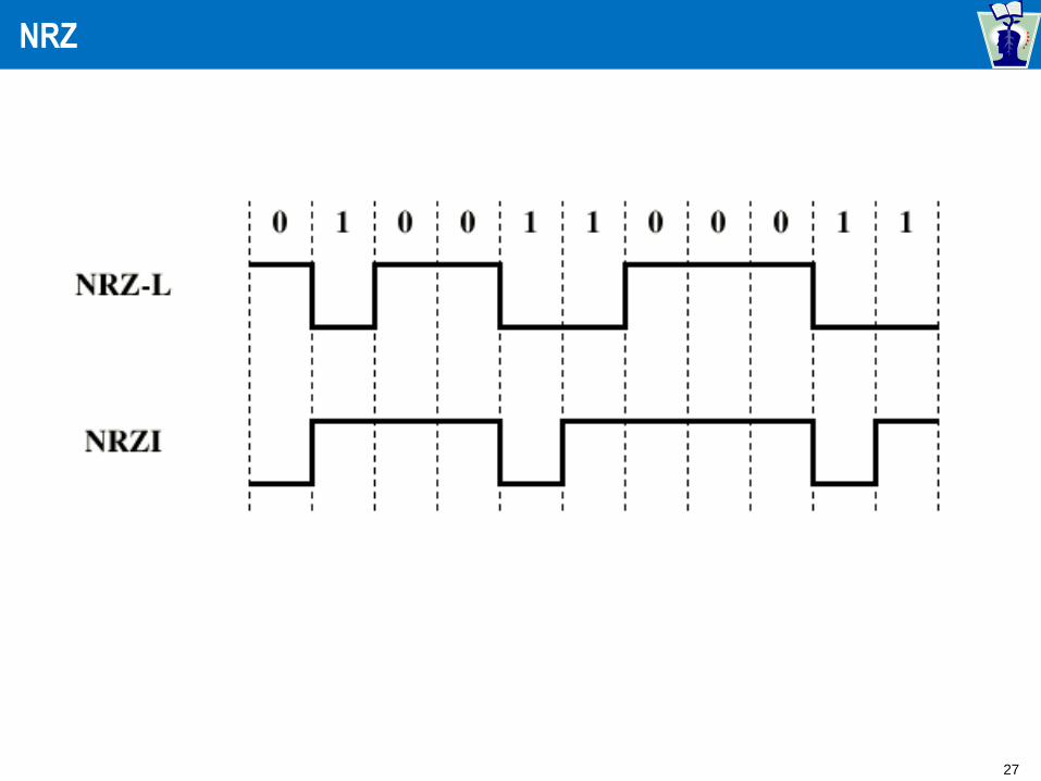
Non-Return to Zero-Level (NRZ-L)
Two different voltages for 0 and 1 bits
Voltage constant during bit interval
No transition (i.e. no return to zero voltage)
e.g., Absence of voltage for zero, constant
positive voltage for one
More often, negative voltage for one value
and positive for the other
This is NRZ-L

26
Non-Return to Zero Inverted
Nonreturn to zero inverted on ones
Constant voltage pulse for duration of bit
Data encoded as presence or absence of signal
transition at beginning of bit time
Transition (low to high or high to low) denotes a
binary 1
No transition denotes binary 0
An example of differential encoding
27
NRZ

28
Differential Encoding
Data represented by changes rather than
levels
More reliable detection of transition rather
than level
In complex transmission layouts it is easy to
lose sense of polarity

29
Summary of Encodings

30
NRZs Pros and Cons
Pros
Easy to engineer
Make good use of bandwidth
Cons
DC component
Lack of synchronization capability
Used for magnetic recording
Not often used for signal transmission

31
Biphase
Manchester
Transition in middle of each bit period
Transition serves as clock and data
Low to high represents one
High to low represents zero
Used by IEEE 802.3
Differential Manchester
Mid-bit transition is clocking only
Transition at start of a bit period represents zero
No transition at start of a bit period represents one
Note: this is a differential encoding scheme
Used by IEEE 802.5

32
Biphase Pros and Cons
Con
At least one transition per bit time and possibly two
Maximum modulation rate is twice NRZ
Requires more bandwidth
Pros
Synchronization on mid bit transition (self clocking)
No dc component
Error detection
Absence of expected transition
33
Asynchronous/Synchronous Transmission
Timing problems require a mechanism
to synchronize the transmitter and
receiver
Two solutions
Asynchronous
Synchronous

34
Asynchronous
Data transmitted on character at a time
5 to 8 bits
Timing only needs maintaining within
each character
Resync with each character

35
Asynchronous (Diagram)

36
Asynchronous - Behavior
In a steady stream, interval between characters is uniform
(length of stop element)
In idle state, receiver looks for transition 1 to 0
Then samples next seven intervals (char length)
Then looks for next 1 to 0 for next char
Simple
Cheap
Overhead of 2 or 3 bits per char (~20%)
Good for data with large gaps (keyboard)
37
Synchronous – Bit Level
Block of data transmitted without start or stop bits
Clocks must be synchronized
Can use separate clock line
Good over short distances
Subject to impairments
Embed clock signal in data
Manchester encoding
Carrier frequency (analog)

38
Synchronous – Block Level
Need to indicate start and end of block
Use preamble and postamble
e.g. series of SYN (hex 16) characters
e.g. block of 11111111 patterns ending in
11111110
More efficient (lower overhead) than
async

39
Synchronous (diagram)

40
ADTs and Protocol Design
Data Encoding and Transmission - Roadmap
Data Encoding and Transmission Concepts
2 Data Encoding and Transmission

41
Common Issues in Design
When building protocol software, there are
two common problems that designers face:
1) How to handle data that arrives from two
independent sources
Down from the higher layer
Up from the lower layer
2) How to implement the protocol

42
Data from Two Sources
Down from the Higher Layer (HL)
Higher layer (HL) sends requests (control and data)
Cannot always process the request immediately, so we
need a place to hold the request
We may get “many” HL users (e.g., many TCP, only
one IP)
Requests may need to be processed out of order (out
of band, QOS, etc)

43
Data from Two Sources
Up from the Lower Layer (LL)
Lower layer sends data and indications
Data must be separated from indications
Read requests from HL may use different data
boundaries than LL
LL may be providing data at same time as HL
wants to read it

44
Ring Buffer of Size N
.
.
.
0
1
2
N-1
Inititial State
Input: 0
Output: 0

45
Ring Buffer of Size N
.
.
.
0
1
2
N-1
New Element
Arrives
Input: 1
Output: 0
Element 0

46
Ring Buffer of Size N
.
.
.
0
1
2
N-1
New Element
Arrives
Input: 2
Output: 0
Element 0
Element 1

47
Ring Buffer of Size N
.
.
.
0
1
2
N-1
Read next
(element 0)
Input: 2
Output: 1
Element 0
Element 1
Read next (element 1)
Input: 2
Output: 2

48
Ring Buffer of Size N
.
.
.
0
1
2
N-1
After Nth
input:
Input: 0
Output: 2
Element 0
Element 1
How many more
input elements can we
accept?
Element 2
Element N-1
49
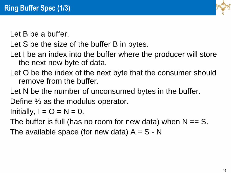
Ring Buffer Spec (1/3)
Let B be a buffer.
Let S be the size of the buffer B in bytes.
Let I be an index into the buffer where the producer will store the next new byte of data.
Let O be the index of the next byte that the consumer should remove from the buffer.
Let N be the number of unconsumed bytes in the buffer.
Define % as the modulus operator.
Initially, I = O = N = 0.
The buffer is full (has no room for new data) when N == S.
The available space (for new data) A = S - N
50
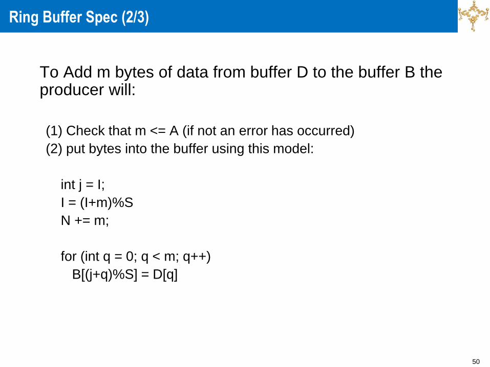
Ring Buffer Spec (2/3)
To Add m bytes of data from buffer D to the buffer B the producer will:
(1) Check that m <= A (if not an error has occurred)
(2) put bytes into the buffer using this model:
int j = I;
I = (I+m)%S
N += m;
for (int q = 0; q < m; q++)
B[(j+q)%S] = D[q]

51
Ring Buffer Spec (3/3)
To remove r bytes from the buffer B to buffer D, the consumer will:
(1) Check that r <= N. If not, adjust r (r = N) or signal error.
(2) take bytes from the buffer using this model:
int j = O;
O = (O+r)%S
N -= r
for (int q = 0; q < r; q++)
D[q] = B[(j+q)%S]

52
Ring Buffer: Making it Safe
So, you see that the idea is that the input (I) and output (O) pointers change continuously from the beginning of the buffer to the end and then wrap around back to the beginning again. Conceptually, it appears as if the end of the buffer is connected back the front of the buffer as if to form a ring (or circle). We enforce that the input pointer never tries to overtake the output pointer!
To make these two methods thread safe, we need only to protect the 3 lines of code that update the class variables O, N, I: NOT the loops that move data! This is a better real-time approach than serializing access to the loop itself, or worse, the entire object.
53
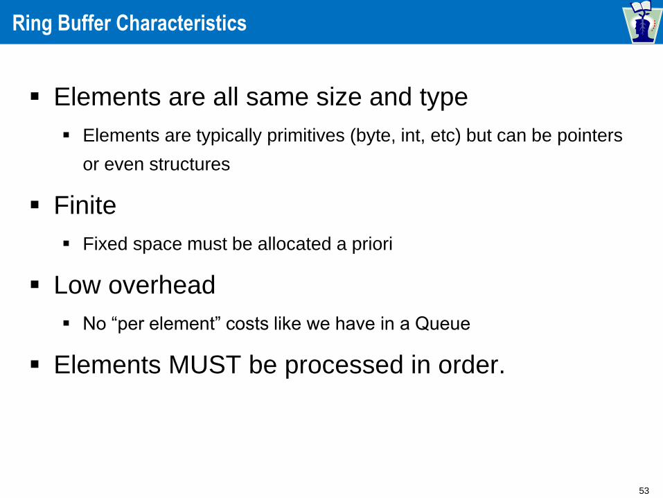
Ring Buffer Characteristics
Elements are all same size and type
Elements are typically primitives (byte, int, etc) but can be pointers
or even structures
Finite
Fixed space must be allocated a priori
Low overhead
No “per element” costs like we have in a Queue
Elements MUST be processed in order.
54
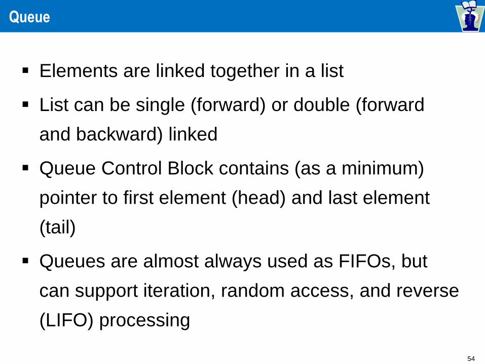
Queue
Elements are linked together in a list
List can be single (forward) or double (forward
and backward) linked
Queue Control Block contains (as a minimum)
pointer to first element (head) and last element
(tail)
Queues are almost always used as FIFOs, but
can support iteration, random access, and reverse
(LIFO) processing

55
Queue (Singly Linked)
head
tail
Queue Control Block
a
z
b z null
element a element b element z
Forward link
Payload
Payload can be ANY object or structure.
Elements need not contain similar payloads.

56
Queue (Doubly Linked)
head
tail
Queue Control Block
a
z
b z null
element a element b element z
b a null
Forward link
Payload
Backward link

57
Queue Operations
Required Operations
Put (add to tail)
Get (get from head)
Nice to Have Operations
Remove (remove specific element)
Insert (add element after a specific element)
Deluxe Operations
Peek (non-destructive Get)
Put to head
Get from tail
Iterate (head to tail or tail to head)

58
Queue Characteristics
Not fixed in length (“unlimited” in length)
Does not require pre-allocated memory
Allows processing of elements in arbitrary
order
Can accommodate elements of different
type
Additional per element cost (links)

59
Queue or Ring Buffer
Stream data: Use a ring buffer
Arriving elements are primitives that make up a
data “stream” (no record boundaries)
TCP data is an example
Service requests: Use a queue
Arriving elements are requests from a user
layer (or clients) and must be processed
individually.

60
What is a FSM?
Let’s define the idea of a “machine”
Organism (real or synthetic) that responds to a
countable (finite) set of stimuli (events) by
generating predictable responses (outputs)
based on a history of prior events (current
state)
A finite state machine (fsm) is a
computational model of a machine

61
FSM Elements
States represent the particular configurations that
our machine can assume
Events define the various inputs that a machine
will recognize
Transitions represent a change of state from a
current state to another (possibly the same) state
that is dependent upon a specific event
The Start State is the state of the machine before
is has received any events

62
Machine Types
Mealy machine
one that generates an output for each transition
Moore machine
one that generates an output for each state
Moore machines can do anything a Mealy
machine can do (and vice versa)
In my experience, Mealy machines are more
useful for implementing communications protocols
The fsm that I’ll provide is a Mealy machine

63
State Diagram

64
From State Diagram to FSM
Identify
States
Events
Transitions
Actions (outputs)
Program these elements into an FSM
Define an event classification process
Drive the events through the FSM
Example ….
65
2 Application Layer
Agenda
1 Session Overview
3 Summary and Conclusion

66
Assignments & Readings
Readings
» Chapters 1 and 5
Assignment #3

67
Next Session: Data Link Control


