1
CS590D: Data MiningChris Clifton
February 24, 2005Concept Description
CS590D 2
Concept Description: Characterization and Comparison
• What is concept description?
• Data generalization and summarization-based characterization
• Analytical characterization: Analysis of attribute relevance
• Mining class comparisons: Discriminating between different classes
• Mining descriptive statistical measures in large databases
• Discussion
• Summary

2
What is Concept Description?
• Descriptive vs. predictive data mining– Descriptive mining: describes concepts or task-
relevant data sets in concise, summarative, informative, discriminative forms
– Predictive mining: Based on data and analysis, constructs models for the database, and predicts the trend and properties of unknown data
• Concept description: – Characterization: provides a concise and succinct
summarization of the given collection of data– Comparison: provides descriptions comparing two or
more collections of data
CS590D 4
Concept Description vs. OLAP
• Concept description: – can handle complex data types of the
attributes and their aggregations– a more automated process
• OLAP: – restricted to a small number of dimension and
measure types– user-controlled process
3
CS590D 5
Concept Description: Characterization and Comparison
• What is concept description? • Data generalization and summarization-based
characterization• Analytical characterization: Analysis of attribute
relevance• Mining class comparisons: Discriminating
between different classes• Mining descriptive statistical measures in large
databases• Discussion• Summary
CS590D 6
Data Generalization and Summarization-based Characterization
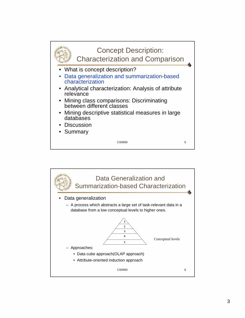
• Data generalization– A process which abstracts a large set of task-relevant data in a
database from a low conceptual levels to higher ones.
– Approaches:
• Data cube approach(OLAP approach)
• Attribute-oriented induction approach
1
2
3
4
5Conceptual levels

4
CS590D 7
Characterization:Data Cube Approach
• Data are stored in data cube• Identify expensive computations
– e.g., count( ), sum( ), average( ), max( )
• Perform computations and store results in data cubes
• Generalization and specialization can be performed on a data cube by roll-up and drill-down
• An efficient implementation of data generalization
CS590D 8
Data Cube Approach (Cont…)
• Limitations– can only handle data types of dimensions to
simple nonnumeric data and of measures tosimple aggregated numeric values.
– Lack of intelligent analysis, can’t tell which dimensions should be used and what levels should the generalization reach
5
CS590D 9
Attribute-Oriented Induction
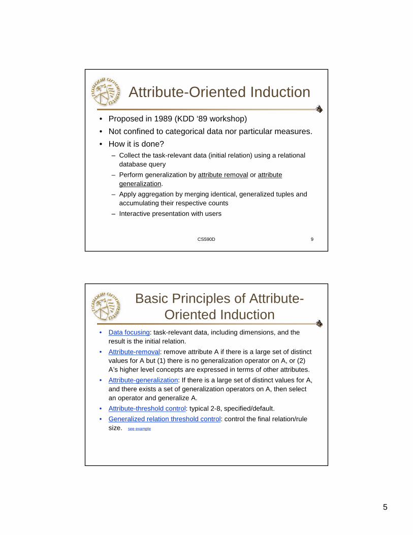
• Proposed in 1989 (KDD ‘89 workshop)
• Not confined to categorical data nor particular measures.
• How it is done?– Collect the task-relevant data (initial relation) using a relational
database query
– Perform generalization by attribute removal or attribute generalization.
– Apply aggregation by merging identical, generalized tuples and accumulating their respective counts
– Interactive presentation with users
Basic Principles of Attribute-Oriented Induction
• Data focusing: task-relevant data, including dimensions, and the result is the initial relation.
• Attribute-removal: remove attribute A if there is a large set of distinct values for A but (1) there is no generalization operator on A, or (2) A’s higher level concepts are expressed in terms of other attributes.
• Attribute-generalization: If there is a large set of distinct values for A, and there exists a set of generalization operators on A, then select an operator and generalize A.
• Attribute-threshold control: typical 2-8, specified/default.
• Generalized relation threshold control: control the final relation/rule size. see example

6
Attribute-Oriented Induction: Basic Algorithm
• InitialRel: Query processing of task-relevant data, deriving the initial relation.
• PreGen: Based on the analysis of the number of distinct values in each attribute, determine generalization plan for each attribute: removal? or how high to generalize?
• PrimeGen: Based on the PreGen plan, perform generalization to the right level to derive a “prime generalized relation”, accumulating the counts.
• Presentation: User interaction: (1) adjust levels by drilling, (2) pivoting, (3) mapping into rules, cross tabs, visualization presentations.
CS590D 12
Example
• DMQL: Describe general characteristics of graduate students in the Big-University databaseuse Big_University_DBmine characteristics as “Science_Students”in relevance to name, gender, major, birth_place, birth_date,
residence, phone#, gpafrom studentwhere status in “graduate”
• Corresponding SQL statement:Select name, gender, major, birth_place, birth_date, residence,
phone#, gpafrom studentwhere status in {“Msc”, “MBA”, “PhD” }
7
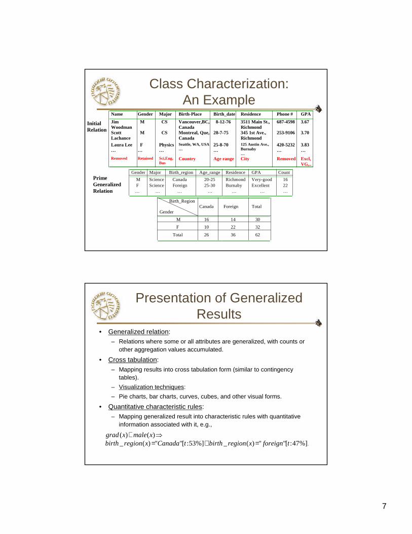
Class Characterization:An Example
Name Gender Major Birth-Place Birth_date Residence Phone # GPA
JimWoodman
M CS Vancouver,BC,Canada
8-12-76 3511 Main St.,Richmond
687-4598 3.67
ScottLachance
M CS Montreal, Que,Canada
28-7-75 345 1st Ave.,Richmond
253-9106 3.70
Laura Lee…
F…
Physics…
Seattle, WA, USA…
25-8-70…
125 Austin Ave.,Burnaby…
420-5232…
3.83…
Removed Retained Sci,Eng,Bus
Country Age range City Removed Excl,VG,..
Gender Major Birth_region Age_range Residence GPA Count
M Science Canada 20-25 Richmond Very-good 16 F Science Foreign 25-30 Burnaby Excellent 22 … … … … … … …
Birth_Region
GenderCanada Foreign Total
M 16 14 30
F 10 22 32
Total 26 36 62
Prime Generalized Relation
Initial Relation
Presentation of Generalized Results
• Generalized relation: – Relations where some or all attributes are generalized, with counts or
other aggregation values accumulated.
• Cross tabulation:– Mapping results into cross tabulation form (similar to contingency
tables).
– Visualization techniques:
– Pie charts, bar charts, curves, cubes, and other visual forms.
• Quantitative characteristic rules:– Mapping generalized result into characteristic rules with quantitative
information associated with it, e.g.,
.%]47:["")(_%]53:["")(_)()(
tforeignxregionbirthtCanadaxregionbirthxmalexgrad
=∨=⇒∧
8
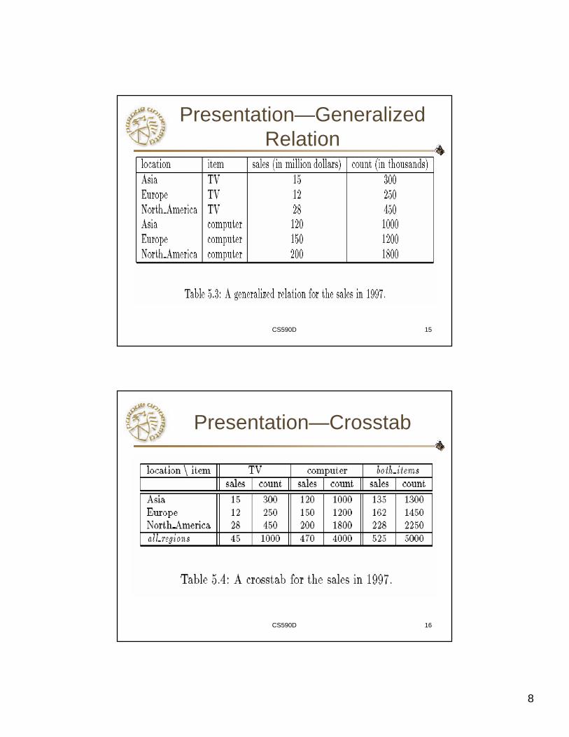
CS590D 15
Presentation—Generalized Relation
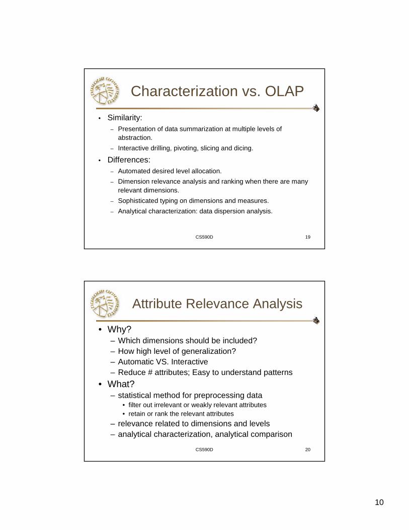
CS590D 16
Presentation—Crosstab

9
CS590D 17
Implementation by Cube Technology
• Construct a data cube on-the-fly for the given data mining query– Facilitate efficient drill-down analysis– May increase the response time– A balanced solution: precomputation of “subprime” relation
• Use a predefined & precomputed data cube– Construct a data cube beforehand– Facilitate not only the attribute-oriented induction, but also
attribute relevance analysis, dicing, slicing, roll-up and drill-down– Cost of cube computation and the nontrivial storage overhead
CS590D 18
Concept Description: Characterization and Comparison
• What is concept description?
• Data generalization and summarization-based characterization
• Analytical characterization: Analysis of attribute relevance
• Mining class comparisons: Discriminating between different classes
• Mining descriptive statistical measures in large databases
• Discussion
• Summary
10
CS590D 19
Characterization vs. OLAP
• Similarity:– Presentation of data summarization at multiple levels of
abstraction.
– Interactive drilling, pivoting, slicing and dicing.
• Differences:– Automated desired level allocation.
– Dimension relevance analysis and ranking when there are many relevant dimensions.
– Sophisticated typing on dimensions and measures.
– Analytical characterization: data dispersion analysis.
CS590D 20
Attribute Relevance Analysis
• Why?– Which dimensions should be included? – How high level of generalization?– Automatic VS. Interactive– Reduce # attributes; Easy to understand patterns
• What?– statistical method for preprocessing data
• filter out irrelevant or weakly relevant attributes • retain or rank the relevant attributes
– relevance related to dimensions and levels– analytical characterization, analytical comparison

11
CS590D 21
Attribute relevance analysis (cont’d)
• How?– Data Collection– Analytical Generalization
• Use information gain analysis (e.g., entropy or other measures) to identify highly relevant dimensions and levels.
– Relevance Analysis• Sort and select the most relevant dimensions and levels.
– Attribute-oriented Induction for class description• On selected dimension/level
– OLAP operations (e.g. drilling, slicing) on relevance rules
CS590D 22
Relevance Measures
• Quantitative relevance measure determines the classifying power of an attribute within a set of data.
• Methods– information gain (ID3)– gain ratio (C4.5)– gini index– χ2 contingency table statistics– uncertainty coefficient
12
CS590D 23
Information-Theoretic Approach
• Decision tree– each internal node tests an attribute– each branch corresponds to attribute value– each leaf node assigns a classification
• ID3 algorithm– build decision tree based on training objects with
known class labels to classify testing objects– rank attributes with information gain measure– minimal height
• the least number of tests to classify an object
CS590D 26
Example:Analytical Characterization
• Task– Mine general characteristics describing graduate
students using analytical characterization
• Given– attributes name, gender, major, birth_place,
birth_date, phone#, and gpa– Gen(ai) = concept hierarchies on ai
– Ui = attribute analytical thresholds for ai
– Ti = attribute generalization thresholds for ai
– R = attribute relevance threshold
13
CS590D 27
Example: Analytical Characterization (cont’d)
• 1. Data collection– target class: graduate student– contrasting class: undergraduate student
• 2. Analytical generalization using Ui– attribute removal
• remove name and phone#
– attribute generalization• generalize major, birth_place, birth_date and gpa• accumulate counts
– candidate relation: gender, major, birth_country, age_range and gpa
28
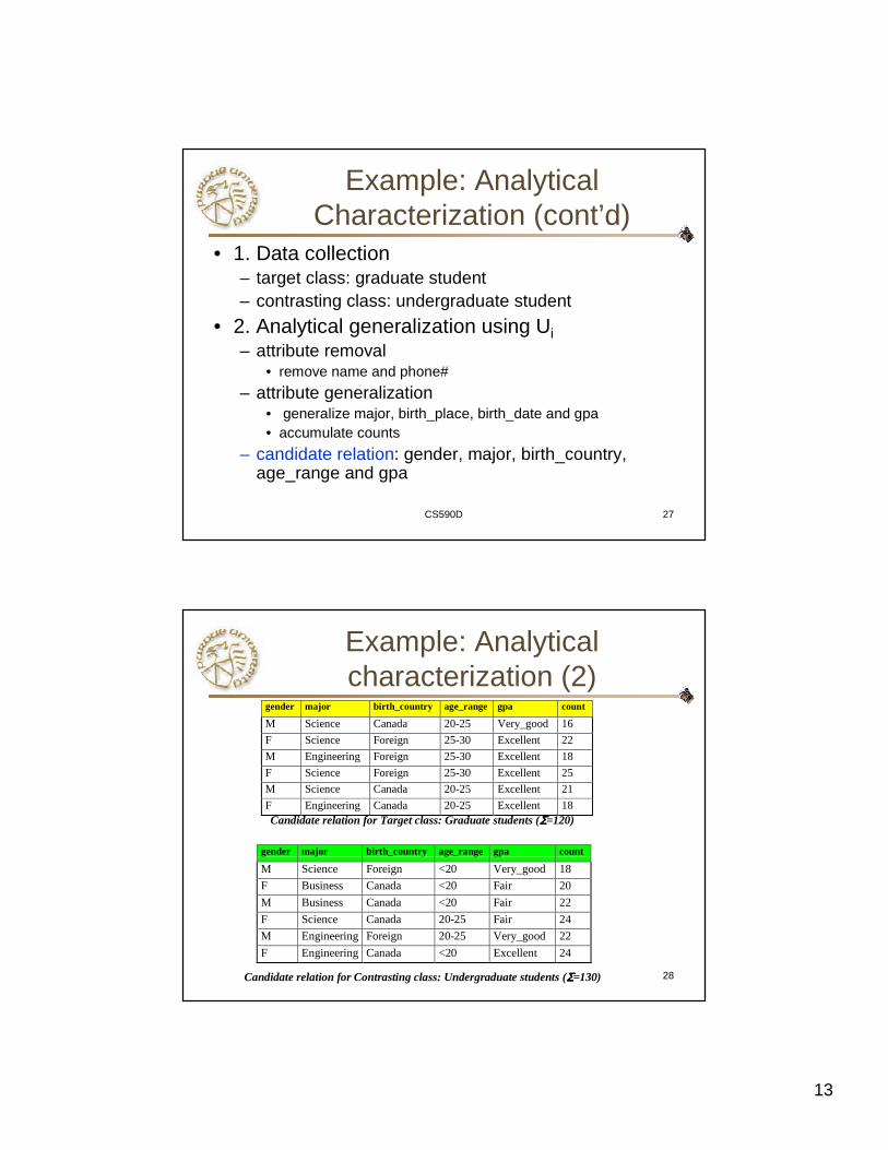
Example: Analytical characterization (2)
gender major birth_country age_range gpa count
M Science Canada 20-25 Very_good 16
F Science Foreign 25-30 Excellent 22
M Engineering Foreign 25-30 Excellent 18
F Science Foreign 25-30 Excellent 25
M Science Canada 20-25 Excellent 21
F Engineering Canada 20-25 Excellent 18Candidate relation for Target class: Graduate students (ΣΣΣΣ=120)
gender major birth_country age_range gpa count
M Science Foreign <20 Very_good 18
F Business Canada <20 Fair 20
M Business Canada <20 Fair 22
F Science Canada 20-25 Fair 24
M Engineering Foreign 20-25 Very_good 22
F Engineering Canada <20 Excellent 24
Candidate relation for Contrasting class: Undergraduate students (ΣΣΣΣ=130)

14
CS590D 29
Example: Analytical characterization (3)
• 3. Relevance analysis– Calculate expected info required to classify an
arbitrary tuple
– Calculate entropy of each attribute: e.g. major
99880250
130
250
130
250
120
250
120130120 2221 .loglog),I()s,I(s =−−==
For major=”Science”: S11=84 S21=42 I(s11,s21)=0.9183
For major=”Engineering”: S12=36 S22=46 I(s12,s22)=0.9892
For major=”Business”: S13=0 S23=42 I(s13,s23)=0
Number of grad students in “Science” Number of undergrad
students in “Science”
CS590D 30
Example: Analytical Characterization (4)
• Calculate expected info required to classify a given sample if S is partitioned according to the attribute
• Calculate information gain for each attribute
– Information gain for all attributes
78730250
42
250
82
250
126231322122111 .)s,s(I)s,s(I)s,s(IE(major) =++=
2115021 .E(major))s,I(s)Gain(major =−=
Gain(gender) = 0.0003
Gain(birth_country) = 0.0407
Gain(major) = 0.2115
Gain(gpa) = 0.4490
Gain(age_range) = 0.5971
15
CS590D 31
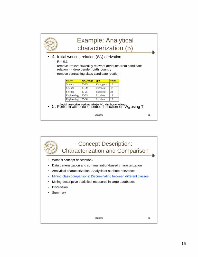
Example: Analytical characterization (5)
• 4. Initial working relation (W0) derivation– R = 0.1– remove irrelevant/weakly relevant attributes from candidate
relation => drop gender, birth_country– remove contrasting class candidate relation
• 5. Perform attribute-oriented induction on W0 using Ti
major age_range gpa countScience 20-25 Very_good 16
Science 25-30 Excellent 47
Science 20-25 Excellent 21
Engineering 20-25 Excellent 18
Engineering 25-30 Excellent 18
Initial target class working relation W0: Graduate students
CS590D 32
Concept Description: Characterization and Comparison
• What is concept description?
• Data generalization and summarization-based characterization
• Analytical characterization: Analysis of attribute relevance
• Mining class comparisons: Discriminating between different classes
• Mining descriptive statistical measures in large databases
• Discussion
• Summary
16
Mining Class Comparisons
• Comparison: Comparing two or more classes
• Method:– Partition the set of relevant data into the target class and the contrasting
class(es)
– Generalize both classes to the same high level concepts
– Compare tuples with the same high level descriptions
– Present for every tuple its description and two measures
• support - distribution within single class
• comparison - distribution between classes
– Highlight the tuples with strong discriminant features
• Relevance Analysis:– Find attributes (features) which best distinguish different classes
CS590D 34
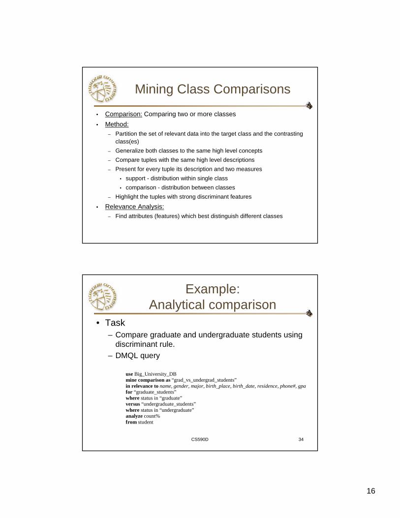
Example:Analytical comparison
• Task– Compare graduate and undergraduate students using
discriminant rule.– DMQL query
useBig_University_DBmine comparison as“grad_vs_undergrad_students”in relevance toname, gender, major, birth_place, birth_date, residence, phone#, gpafor “graduate_students”where status in “graduate”versus“undergraduate_students”where status in “undergraduate”analyzecount%from student

17
CS590D 35
Example: Analytical comparison (2)
• Given– attributes name, gender, major, birth_place,
birth_date, residence, phone# and gpa– Gen(ai) = concept hierarchies on attributes ai
– Ui = attribute analytical thresholds for attributes ai
– Ti = attribute generalization thresholds for attributes ai
– R = attribute relevance threshold
CS590D 36
Example: Analytical comparison (3)
• 1. Data collection– target and contrasting classes
• 2. Attribute relevance analysis– remove attributes name, gender, major, phone#
• 3. Synchronous generalization– controlled by user-specified dimension thresholds– prime target and contrasting class(es)
relations/cuboids

18
37
Example: Analytical comparison (4)
Birth_country Age_range Gpa Count%Canada 20-25 Good 5.53%
Canada 25-30 Good 2.32%
Canada Over_30 Very_good 5.86%
… … … …
Other Over_30 Excellent 4.68%Prime generalized relation for the target class: Graduate students
Birth_country Age_range Gpa Count%Canada 15-20 Fair 5.53%
Canada 15-20 Good 4.53%
… … … …
Canada 25-30 Good 5.02%
… … … …
Other Over_30 Excellent 0.68%
Prime generalized relation for the contrasting class: Undergraduate students
CS590D 38
Example: Analytical comparison (5)
• 4. Drill down, roll up and other OLAP operations on target and contrasting classes to adjust levels of abstractions of resulting description
• 5. Presentation– as generalized relations, crosstabs, bar
charts, pie charts, or rules– contrasting measures to reflect comparison
between target and contrasting classes• e.g. count%
19
CS590D 39
Quantitative DiscriminantRules
• Cj = target class• qa = a generalized tuple covers some tuples of
class– but can also cover some tuples of contrasting class
• d-weight– range: [0, 1]
• quantitative discriminant rule form
∑=
∈
∈=− m
i
ia
ja
)Ccount(q
)Ccount(qweightd
1
d_weight]:[dX)condition(ss(X)target_claX, ⇐∀
CS590D 40
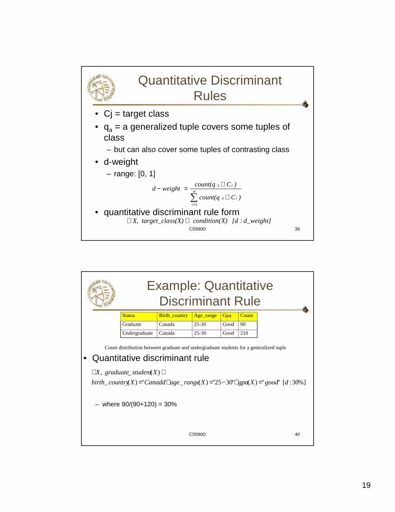
Example: Quantitative Discriminant Rule
• Quantitative discriminant rule
– where 90/(90+120) = 30%
Status Birth_country Age_range Gpa Count
Graduate Canada 25-30 Good 90
Undergraduate Canada 25-30 Good 210
Count distribution between graduate and undergraduate students for a generalized tuple
%]30:["")("3025")(_"")(_
)(_,
dgoodXgpaXrangeageCanadaXcountrybirth
XstudentgraduateX
=∧−=∧=⇐∀
20
CS590D: Data MiningChris Clifton
March 1, 2005Concept Description
CS590D 42
Class Description
• Quantitative characteristic rule
– necessary
• Quantitative discriminant rule
– sufficient
• Quantitative description rule
– necessary and sufficient
]w:d,w:[t...]w:d,w:[t nn111 ′∨∨′⇔∀
(X)condition(X)condition
ss(X)target_claX,
n
d_weight]:[dX)condition(ss(X)target_claX, ⇐∀
t_weight]:[tX)condition(ss(X)target_claX, ⇒∀
21
CS590D 43
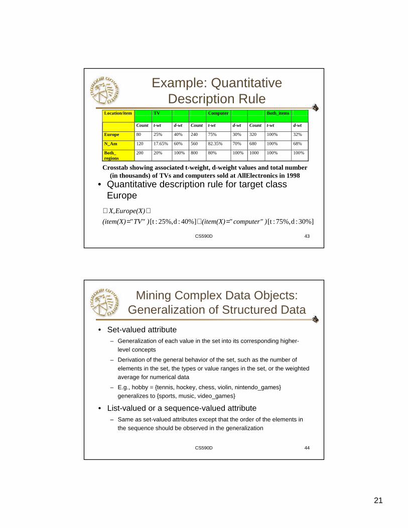
Example: Quantitative Description Rule
• Quantitative description rule for target class Europe
Location/item TV Computer Both_items
Count t-wt d-wt Count t-wt d-wt Count t-wt d-wt
Europe 80 25% 40% 240 75% 30% 320 100% 32%
N_Am 120 17.65% 60% 560 82.35% 70% 680 100% 68%
Both_ regions
200 20% 100% 800 80% 100% 1000 100% 100%
Crosstab showing associated t-weight, d-weight values and total number (in thousands) of TVs and computers sold at AllElectronics in 1998
30%]:d75%,:[t40%]:d25%,:[t )computer""(item(X))TV""(item(X)
Europe(X)X,
=∨=⇔∀
CS590D 44
Mining Complex Data Objects: Generalization of Structured Data
• Set-valued attribute– Generalization of each value in the set into its corresponding higher-
level concepts
– Derivation of the general behavior of the set, such as the number of
elements in the set, the types or value ranges in the set, or the weighted average for numerical data
– E.g., hobby = {tennis, hockey, chess, violin, nintendo_games} generalizes to {sports, music, video_games}
• List-valued or a sequence-valued attribute– Same as set-valued attributes except that the order of the elements in
the sequence should be observed in the generalization
22
CS590D 45
Generalizing Spatial and Multimedia Data
• Spatial data:– Generalize detailed geographic points into clustered regions, such as
business, residential, industrial, or agricultural areas, according to land usage
– Require the merge of a set of geographic areas by spatial operations
• Image data:– Extracted by aggregation and/or approximation– Size, color, shape, texture, orientation, and relative positions and
structures of the contained objects or regions in the image
• Music data: – Summarize its melody: based on the approximate patterns that
repeatedly occur in the segment– Summarized its style: based on its tone, tempo, or the major musical
instruments played
CS590D 46
Generalizing Object Data• Object identifier: generalize to the lowest level of class in the
class/subclass hierarchies• Class composition hierarchies
– generalize nested structured data– generalize only objects closely related in semantics to the current one
• Construction and mining of object cubes– Extend the attribute-oriented induction method
• Apply a sequence of class-based generalization operators on different attributes
• Continue until getting a small number of generalized objects that can be summarized as a concise in high-level terms
– For efficient implementation • Examine each attribute, generalize it to simple-valued data • Construct a multidimensional data cube (object cube)• Problem: it is not always desirable to generalize a set of values to
single-valued data

23
CS590D 47
An Example: Plan Mining by Divide & Conquer
• Plan: a variable sequence of actions– E.g., Travel (flight): <traveler, departure, arrival, d-time, a-time, airline, price,
seat>
• Plan mining: extraction of important or significant generalized (sequential) patterns from a planbase (a large collection of plans)– E.g., Discover travel patterns in an air flight database, or
– find significant patterns from the sequences of actions in the repair of automobiles
• Method– Attribute-oriented induction on sequence data
• A generalized travel plan: <small-big*-small>
– Divide & conquer:Mine characteristics for each subsequence
• E.g., big*: same airline, small-big: nearby region
CS590D 48
A Travel Database for Plan Mining
• Example: Mining a travel plan baseplan# action# departure depart_time arrival arrival_time airline …1 1 ALB 800 JFK 900 TWA …1 2 JFK 1000 ORD 1230 UA …1 3 ORD 1300 LAX 1600 UA …1 4 LAX 1710 SAN 1800 DAL …2 1 SPI 900 ORD 950 AA …. . . . . . . .. . . . . . . .. . . . . . . .
airport_code city state region airport_size …1 1 ALB 800 …1 2 JFK 1000 …1 3 ORD 1300 …1 4 LAX 1710 …2 1 SPI 900 …. . . . .. . . . .. . . . .
Travel plans table
Airport info table

24
CS590D 49
Multidimensional Analysis
• Strategy– Generalize the plan
base in different directions
– Look for sequential patterns in the generalized plans
– Derive high-level plans
A multi-D model for the plan base
CS590D 50
Multidimensional Generalization
Plan# Loc_Seq Size_Seq State_Seq 1 ALB - JFK - ORD - LAX - SAN S - L - L - L - S N - N - I - C - C2 SPI - ORD - JFK - SYR S - L - L - S I - I - N - N. . .. . .. . .
Multi-D generalization of the plan base
Plan# Size_Seq State_Seq Region_Seq …1 S - L+ - S N+ - I - C+ E+ - M - P+ …2 S - L+ - S I+ - N+ M+ - E+ …. . .. . .. . .
Merging consecutive, identical actions in plans
%]75[)()(),(_),(_),,(
yregionxregion
LysizeairportSxsizeairportyxflight
=⇒
∧∧

25
CS590D 51
Generalization-Based Sequence Mining
• Generalize planbase in multidimensional way using dimension tables
• Use # of distinct values (cardinality) at each level to determine the right level of generalization (level-“planning”)
• Use operators merge “+”, option “[]” to further generalize patterns
• Retain patterns with significant support
CS590D 52
Generalized Sequence Patterns
• AirportSize-sequence survives the min threshold (after applying merge operator):
S-L+-S [35%], L+-S [30%], S-L+ [24.5%], L+ [9%]
• After applying option operator:
[S] -L+-[S] [98.5%]
– Most of the time, people fly via large airports to get to final
destination
• Other plans: 1.5% of chances, there are other patterns: S-S, L-S-L

26
CS590D 53
Concept Description: Characterization and Comparison
• What is concept description?
• Data generalization and summarization-based characterization
• Analytical characterization: Analysis of attribute relevance
• Mining class comparisons: Discriminating between different classes
• Mining descriptive statistical measures in large databases
• Discussion
• Summary
CS590D 54
Mining Data Dispersion Characteristics
• Motivation– To better understand the data: central tendency, variation and spread
• Data dispersion characteristics– median, max, min, quantiles, outliers, variance, etc.
• Numerical dimensions correspond to sorted intervals– Data dispersion: analyzed with multiple granularities of precision
– Boxplot or quantile analysis on sorted intervals
• Dispersion analysis on computed measures– Folding measures into numerical dimensions
– Boxplot or quantile analysis on the transformed cube

27
CS590D 55
Measuring the Central Tendency
• Mean
– Weighted arithmetic mean
• Median: A holistic measure
– Middle value if odd number of values, or average of the middle two
values otherwise
– estimated by interpolation
• Mode
– Value that occurs most frequently in the data
– Unimodal, bimodal, trimodal
– Empirical formula:
∑=
=n
iix
nx
1
1
∑
∑
=
==n
ii
n
iii
w
xwx
1
1
cf
lfnLmedian
median
))(2/
(1∑−
+=
)(3 medianmeanmodemean −×=−
CS590D 56
Measuring the Dispersion of Data
• Quartiles, outliers and boxplots
– Quartiles: Q1 (25th percentile), Q3 (75th percentile)
– Inter-quartile range: IQR = Q3 – Q1
– Five number summary: min, Q1, M, Q3, max
– Boxplot: ends of the box are the quartiles, median is marked, whiskers,and plot outlier individually
– Outlier: usually, a value higher/lower than 1.5 x IQR
• Variance and standard deviation
– Variance s2: (algebraic, scalable computation)
– Standard deviation s is the square root of variance s2
∑ ∑∑= ==
−−
=−−
=n
i
n
iii
n
ii x
nx
nxx
ns
1 1
22
1
22 ])(1
[1
1)(
1
1
28
CS590D 57
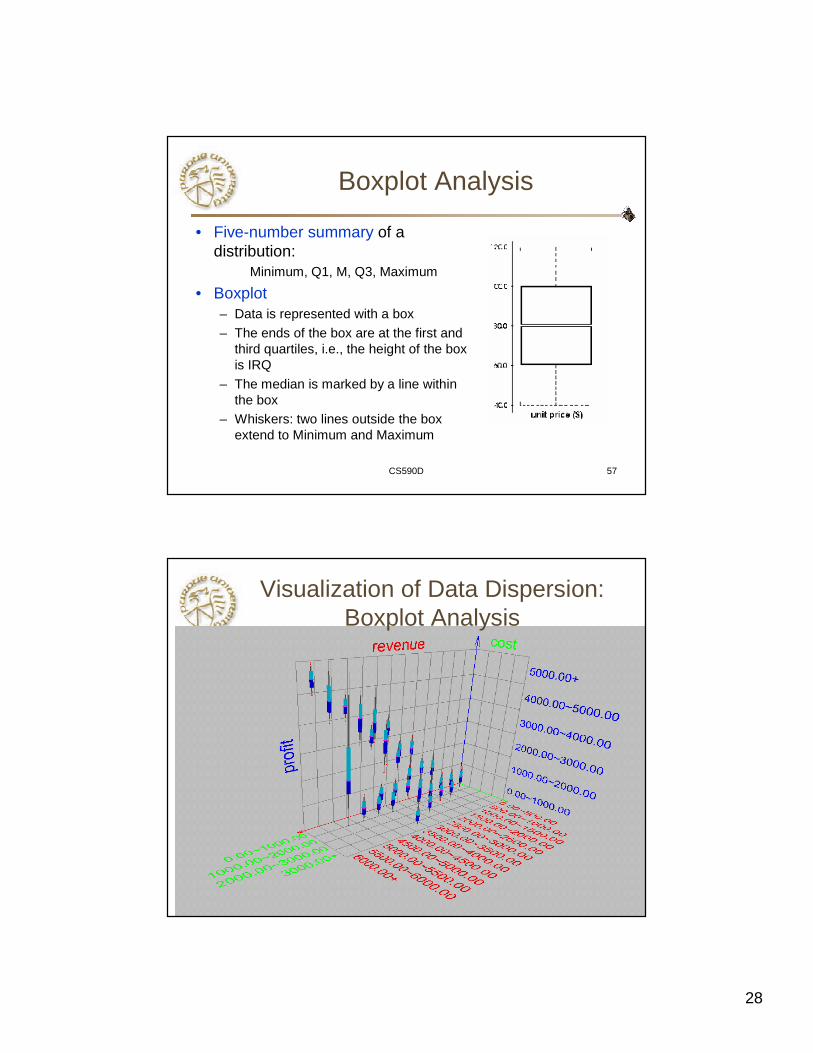
Boxplot Analysis
• Five-number summary of a distribution:
Minimum, Q1, M, Q3, Maximum
• Boxplot– Data is represented with a box
– The ends of the box are at the first and third quartiles, i.e., the height of the box is IRQ
– The median is marked by a line within the box
– Whiskers: two lines outside the box extend to Minimum and Maximum
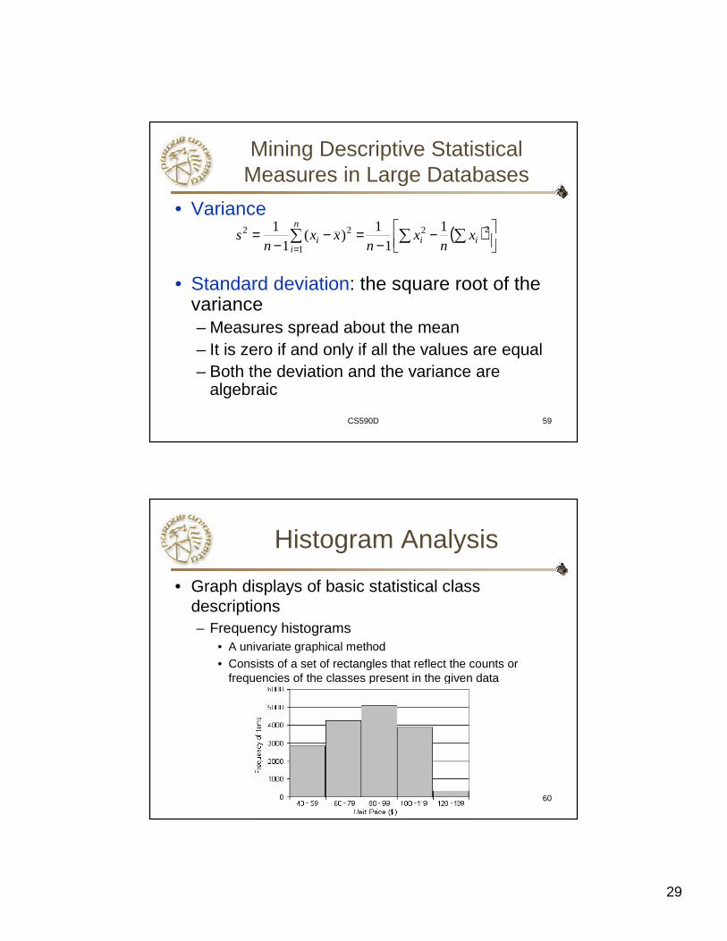
CS590D 58
Visualization of Data Dispersion: Boxplot Analysis
29
CS590D 59
Mining Descriptive Statistical Measures in Large Databases
• Variance
• Standard deviation: the square root of the variance– Measures spread about the mean– It is zero if and only if all the values are equal– Both the deviation and the variance are
algebraic
( )
−−
=−−
= ∑ ∑∑=
22
1
22 11
1)(
11
ii
n
ii x
nx
nxx
ns
CS590D 60
Histogram Analysis
• Graph displays of basic statistical class descriptions– Frequency histograms
• A univariate graphical method
• Consists of a set of rectangles that reflect the counts or frequencies of the classes present in the given data
30
CS590D 61
Graphic Displays of Basic Statistical Descriptions
• Histogram: (shown before)• Boxplot: (covered before)• Quantile plot: each value xi is paired with fi indicating
that approximately 100 fi % of data are ≤ xi
• Quantile-quantile (q-q) plot: graphs the quantiles of one univariant distribution against the corresponding quantiles of another
• Scatter plot: each pair of values is a pair of coordinates and plotted as points in the plane
• Loess (local regression) curve: add a smooth curve to a scatter plot to provide better perception of the pattern of dependence
CS590D 62
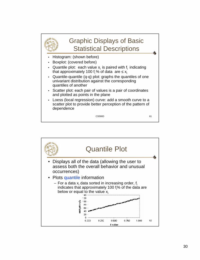
Quantile Plot
• Displays all of the data (allowing the user to assess both the overall behavior and unusual occurrences)
• Plots quantile information– For a data xi data sorted in increasing order, fi
indicates that approximately 100 fi% of the data are below or equal to the value xi
31
CS590D 63
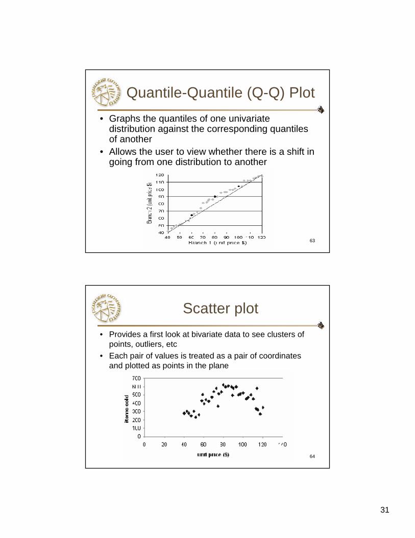
Quantile-Quantile (Q-Q) Plot
• Graphs the quantiles of one univariatedistribution against the corresponding quantilesof another
• Allows the user to view whether there is a shift in going from one distribution to another
CS590D 64
Scatter plot
• Provides a first look at bivariate data to see clusters of points, outliers, etc
• Each pair of values is treated as a pair of coordinates and plotted as points in the plane

32
CS590D 65
Loess Curve
• Adds a smooth curve to a scatter plot in order to provide better perception of the pattern of dependence
• Loess curve is fitted by setting two parameters: a smoothing parameter, and the degree of the polynomials that are fitted by the regression
CS590D 66
Concept Description: Characterization and Comparison
• What is concept description?
• Data generalization and summarization-based characterization
• Analytical characterization: Analysis of attribute relevance
• Mining class comparisons: Discriminating between different classes
• Mining descriptive statistical measures in large databases
• Discussion
• Summary

33
CS590D 67
AO Induction vs. Learning-from-example Paradigm
• Difference in philosophies and basic assumptions– Positive and negative samples in learning-from-example:
positive used for generalization, negative - for specialization
– Positive samples only in data mining: hence generalization-based, to drill-down backtrack the generalization to a previous state
• Difference in methods of generalizations– Machine learning generalizes on a tuple by tuple basis
– Data mining generalizes on an attribute by attribute basis
CS590D 68
Entire vs. Factored Version Space

34
CS590D 69
Incremental and Parallel Mining of Concept Description
• Incremental mining: revision based on newly added data ∆DB– Generalize ∆DB to the same level of abstraction in
the generalized relation R to derive ∆R
– Union R U ∆R, i.e., merge counts and other statistical information to produce a new relation R’
• Similar philosophy can be applied to data sampling, parallel and/or distributed mining, etc.
CS590D 70
Concept Description: Characterization and Comparison
• What is concept description?
• Data generalization and summarization-based characterization
• Analytical characterization: Analysis of attribute relevance
• Mining class comparisons: Discriminating between different classes
• Mining descriptive statistical measures in large databases
• Discussion
• Summary
35
CS590D 71
Summary
• Concept description: characterization and discrimination
• OLAP-based vs. attribute-oriented induction
• Efficient implementation of AOI
• Analytical characterization and comparison
• Mining descriptive statistical measures in large databases
• Discussion
– Incremental and parallel mining of description
– Descriptive mining of complex types of data
CS590D 72
References
• Y. Cai, N. Cercone, and J. Han. Attribute-oriented induction in relational databases. In G. Piatetsky-Shapiro and W. J. Frawley, editors, Knowledge Discovery in Databases, pages 213-228. AAAI/MIT Press, 1991.
• S. Chaudhuri and U. Dayal. An overview of data warehousing and OLAP technology. ACM SIGMOD Record, 26:65-74, 1997
• C. Carter and H. Hamilton. Efficient attribute-oriented generalization for knowledge discovery from large databases. IEEE Trans. Knowledge and Data Engineering, 10:193-208, 1998.
• W. Cleveland. Visualizing Data. Hobart Press, Summit NJ, 1993.• J. L. Devore. Probability and Statistics for Engineering and the Science, 4th ed.
Duxbury Press, 1995.• T. G. Dietterich and R. S. Michalski. A comparative review of selected methods for
learning from examples. In Michalski et al., editor, Machine Learning: An Artificial Intelligence Approach, Vol. 1, pages 41-82. Morgan Kaufmann, 1983.
• J. Gray, S. Chaudhuri, A. Bosworth, A. Layman, D. Reichart, M. Venkatrao, F. Pellow, and H. Pirahesh. Data cube: A relational aggregation operator generalizing group-by, cross-tab and sub-totals. Data Mining and Knowledge Discovery, 1:29-54, 1997.
• J. Han, Y. Cai, and N. Cercone. Data-driven discovery of quantitative rules in relational databases. IEEE Trans. Knowledge and Data Engineering, 5:29-40, 1993.

36
CS590D 73
References (cont.)
• J. Han and Y. Fu. Exploration of the power of attribute-oriented induction in data mining. In U.M. Fayyad, G. Piatetsky-Shapiro, P. Smyth, and R. Uthurusamy, editors, Advances in Knowledge Discovery and Data Mining, pages 399-421. AAAI/MIT Press, 1996.
• R. A. Johnson and D. A. Wichern. Applied Multivariate Statistical Analysis, 3rd ed. Prentice Hall, 1992.
• E. Knorr and R. Ng. Algorithms for mining distance-based outliers in large datasets. VLDB'98, New York, NY, Aug. 1998.
• H. Liu and H. Motoda. Feature Selection for Knowledge Discovery and Data Mining. Kluwer Academic Publishers, 1998.
• R. S. Michalski. A theory and methodology of inductive learning. In Michalski et al., editor, Machine Learning: An Artificial Intelligence Approach, Vol. 1, Morgan Kaufmann, 1983.
• T. M. Mitchell. Version spaces: A candidate elimination approach to rule learning. IJCAI'97, Cambridge, MA.
• T. M. Mitchell. Generalization as search. Artificial Intelligence, 18:203-226, 1982.• T. M. Mitchell. Machine Learning. McGraw Hill, 1997.• J. R. Quinlan. Induction of decision trees. Machine Learning, 1:81-106, 1986.• D. Subramanian and J. Feigenbaum. Factorization in experiment generation.
AAAI'86, Philadelphia, PA, Aug. 1986.


