
Credibility Modeling with Applications
by
Tatiana Khapaeva
Thesis presented in a partial fulfilment of the requirements
for the degree of
Master of Science (M.Sc.) in Computational Sciences
School of Graduate Studies
Laurentian University
Sudbury, Ontario
c© Tatiana Khapaeva, 2014

THESIS DEFENCE COMMITTEE/COMITÉ DE SOUTENANCE DE THÈSE
Laurentian Université/Université Laurentienne
School of Graduate Studies/École des études supérieures
Title of Thesis
Titre de la thèse CREDIBILITY MODELING WITH APPLICATIONS
Name of Candidate
Nom du candidat Khapaeva, Tatiana
Degree
Diplôme Master of Science
Department/Program Date of Defence
Département/Programme Computational Sciences Date de la soutenance April 22, 2014
APPROVED/APPROUVÉ
Thesis Examiners/Examinateurs de thèse:
Dr. Peter Adamic
(Supervisor/Directeur de thèse)
Prof. Michael Herman
(Committee member/Membre du comité)
Approved for the School of Graduate Studies
Dr. Ratvinder Grewal Approuvé pour l’École des études supérieures
(Committee member/Membre du comité) Dr. David Lesbarrères
M. David Lesbarrères
Dr. Natalia Stepanova Director, School of Graduate Studies
(External Examiner/Examinatrice externe) Directeur, École des études supérieures
ACCESSIBILITY CLAUSE AND PERMISSION TO USE
I, Tatiana Khapaeva, hereby grant to Laurentian University and/or its agents the non-exclusive license to archive
and make accessible my thesis, dissertation, or project report in whole or in part in all forms of media, now or for the
duration of my copyright ownership. I retain all other ownership rights to the copyright of the thesis, dissertation or
project report. I also reserve the right to use in future works (such as articles or books) all or part of this thesis,
dissertation, or project report. I further agree that permission for copying of this thesis in any manner, in whole or in
part, for scholarly purposes may be granted by the professor or professors who supervised my thesis work or, in their
absence, by the Head of the Department in which my thesis work was done. It is understood that any copying or
publication or use of this thesis or parts thereof for financial gain shall not be allowed without my written
permission. It is also understood that this copy is being made available in this form by the authority of the copyright
owner solely for the purpose of private study and research and may not be copied or reproduced except as permitted
by the copyright laws without written authority from the copyright owner.

Abstract
The purpose of this thesis is to show how the theory and practice of credibility
can benefit statistical modeling. The task was, fundamentally, to derive models that
could provide the best estimate of the losses for any given class and also to assess the
variability of the losses, both from a class perspective as well as from an aggregate
perspective. The model fitting and diagnostic tests will be carried out using standard
statistical packages. A case study that predicts the number of deaths due to cancer is
considered, utilizing data furnished by the Colorado Department of Public Health and
Environment. Several credibility models are used, including Bayesian, Buhlmann and
Buhlmann-Straub approaches, which are useful in a wide range of actuarial applications.
iii

Contents
1 Introduction 1
2 The Concept of Credibility 3
3 The Bayesian Credibility Model 10
3.1 Bayesian estimation . . . . . . . . . . . . . . . . . . . . . . . . . . . . . . 10
3.2 Derivation of the Bayesian Credibility Model . . . . . . . . . . . . . . . . 14
3.3 Conjugate Priors in Bayesian Credibility . . . . . . . . . . . . . . . . . . 19
4 The Buhlmann Credibility Model 22
4.1 Target Shooting Example . . . . . . . . . . . . . . . . . . . . . . . . . . 22
4.2 Credibility Parameters . . . . . . . . . . . . . . . . . . . . . . . . . . . . 27
4.3 Derivation of the Buhlmann Credibility Model . . . . . . . . . . . . . . . 31
5 The Buhlmann - Straub Credibility Model 36
5.1 Credibility Parameters . . . . . . . . . . . . . . . . . . . . . . . . . . . . 36
5.2 Nonparametric Estimation . . . . . . . . . . . . . . . . . . . . . . . . . . 39
6 An Analysis of Colorado Cancer Death Rates 42
iv

6.1 Introduction to the Cancer Data Set . . . . . . . . . . . . . . . . . . . . 42
6.2 Regression Model Diagnostics . . . . . . . . . . . . . . . . . . . . . . . . 48
6.3 Analysis of Results . . . . . . . . . . . . . . . . . . . . . . . . . . . . . . 51
7 Conclusion 54
References 60
Appendices 62
v

List of Tables
6.1 Denver County Deaths by Cancer Data Set . . . . . . . . . . . . . . . . . 43
6.2 Non-Denver Deaths by Cancer Data Set . . . . . . . . . . . . . . . . . . 43
6.3 Table of Results for Denver County . . . . . . . . . . . . . . . . . . . . . 46
6.4 Table of Results for Non-Denver . . . . . . . . . . . . . . . . . . . . . . . 47
6.5 Table of Year - Predicted Crude Death Rate Estimates . . . . . . . . . . 47
6.6 Summary Statistics for Denver County Dataset . . . . . . . . . . . . . . 50
6.7 Results for the Denver County Dataset . . . . . . . . . . . . . . . . . . . 52
vi

List of Figures
4.1 Target Shooting Figure 1 . . . . . . . . . . . . . . . . . . . . . . . . . . . 23
4.2 Target Shooting Figure 2 . . . . . . . . . . . . . . . . . . . . . . . . . . . 24
4.3 Target Shooting Figure 3 . . . . . . . . . . . . . . . . . . . . . . . . . . . 25
6.1 Linear Regression Scatterplot for Denver County . . . . . . . . . . . . . . 49
6.2 Residuals vs. Fitted values plot for Denver County . . . . . . . . . . . . 51
7.1 Excel Calculation Sheet . . . . . . . . . . . . . . . . . . . . . . . . . . . 58
vii

Chapter 1
Introduction
The actuary uses observations of events that happened in the past to forecast future
events or costs. For example, data that was collected over several years about the
average cost to insure a selected risk, sometimes referred to as a policyholder or insured,
may be used to estimate the expected cost to insure the same risk in future years.
Because insured losses arise from random occurrences, however, the actual costs of paying
insurance losses in past years may be a poor estimator of future costs. The insurer is
then forced to answer the following questions: how credible is the policyholder’s own
experience? And what weight should be given to the class rate?
Credibility theory began with papers by Mowbray (1914) and Whitney (1918). In
those papers, the emphasis was on deriving a premium which was a balance between
the experience of an individual risk and a class of risks. Buhlmann (1967) showed
how a credibility formula can be derived in a distribution-free way, using a least-squares
criterion. Since then, a number of papers have shown how this approach can be extended.
For example, Buhlmann and Straub (1970), Hachemeister (1975), de Vylder(1976,1986),
Jewell (1974, 1975), and more recently Klugman (1987, 1998), saw the development of
1

linear unbiased estimators to the theoretically exact Bayesian estimates. The credibility
models espoused in the Klugman paper have a prior or collateral information that can
be weighted with current observations. The goal of this approach is the minimization of
the square of the error between the estimate and the true expected value of the quantity
being estimated.
2

Chapter 2
The Concept of Credibility
Credibility Theory is a set of quantitative tools which allows an insurer to perform
prospective experience rating (adjust future premiums based on past experience) on a
risk or group of risks. Credibility provides tools to deal with the randomness of data
that is used for predicting future events or costs. For example, an insurance company
uses past loss information of an insured or group of insureds to estimate the cost to
provide future insurance coverage. But, insurance losses arise from random occurrences.
The average annual cost of paying insurance losses in the past few years may be a poor
estimate of next years costs. The expected accuracy of this estimate is a function of
the variability in the losses. This data by itself may not be acceptable for calculating
insurance rates. Rather than relying solely on recent observations, better estimates may
be obtained by combining this data with other information. For example, suppose that
recent experience indicates that Carpenters should be charged a rate of $5 (per $100 of
payroll) for workers compensation insurance. Assume that the current rate is $10. What
should the new rate be? Should it be $5, $10, or somewhere in between? Credibility is
used to weight together these two estimates.
3

The basic formula for calculating the credibility weighted estimate is:
Estimate = Z × [Observation] + (1− Z)[Other Information], 0 ≤ Z ≤ 1.
Z represents the credibility assigned to the observation. 1 − Z is generally referred to
as the complement of credibility. If the body of observed data is large and not likely to
vary much from one period to another, then Z will be closer to one. On the other hand,
if the observation consists of limited data, then Z will be closer to zero and more weight
will be given to other information.
The current rate of $10 in the above example is the “Other Information”. It rep-
resents an estimate or prior hypothesis of a rate to charge in the absence of the recent
experience. As recent experience becomes available, then an updated estimate combin-
ing the recent experience and the prior hypothesis can be calculated. Thus, the use of
credibility involves a linear estimate of the true expectation derived as a result of a com-
promise between observation and the prior hypothesis. The Carpenters rate for workers
compensation insurance is Z · $5 + (1− Z) · $10 under this model.
The following is another example demonstrating how credibility can help produce
better estimates.
Example 1:
In a large population of automobile drivers, the average driver has one accident
every five years or, equivalently, an annual frequency of .20 accidents per year. A driver
selected randomly from the population had three accidents during the last five years for
4

a frequency of .60 accidents per year. What will be the estimate of the expected future
frequency rate for this driver? Is it .20, .60, or something in between?
Solution:
If we had no information about the driver other than that he came from the popula-
tion, we should go with the .20. However, we know that the driver’s observed frequency
was .60. Should this be our estimate for his future accident frequency? Probably not.
There is a correlation between prior accident frequency and future accident frequency,
but they are not perfectly correlated. Accidents occur randomly and even good drivers
with low expected accident frequencies will have accidents. On the other hand, bad
drivers can go several years without an accident. A better answer than either .20 or .60
is most likely something in between: this driver’s Expected Future Accident Frequency
is F = Z · 0.60 + (1− Z) · 0.20. �
Consider a risk that is a member of a particular class of risks. Classes are groupings of
risks with similar risk characteristics, and though similar, each risk is still unique and not
quite the same as other risks in the class. In class rating, the insurance premium charged
to each risk in a class is derived from a rate common to the class. Class rating is often
supplemented with experience rating so that the insurance premium for an individual risk
is based on both the class rate and actual past loss experience for the risk. The important
question in this case is: How much should the class rate be modified by experience rating?
That is, how much credibility should be given to the actual experience of the individual
risk?
5
Let the probability function (pf) pk denote the probability that exactly “k” events
occur. Let N be a random variable representing the number of such events. Then
pk = Pr(N = k), k = 0, 1, 2, ...
When it is unclear, or when the random variable may be continuous, discrete, or a
mixture of the two, the term probability function and abbreviation pf will be used. The
term probability density function and the abbreviation pdf will be used only when the
random variable is known to be continuous.
Suppose that X and Y are two random variables with joint probability function
(pf) or probability density function (pdf) fX,Y (x, y) and marginal pfs fX(x) and fY (y),
respectively. The conditional pf of X given that Y = y is
fX|Y (x|y) =fX,Y (x|y)
fY (y).
IfX and Y are discrete random variables, then fX|Y (x|y) is the conditional probability
of the event X = x under the hypothesis that Y = y. If X and Y are continuous, then
fX|Y (x|y) may be interpreted as a definition. When X and Y are independent random
variables,
fX,Y (x, y) = fX(x)fY (y)
and in this case fX|Y (x|y) = fX(x), and we observe that the conditional and marginal
distributions of X are identical. Also, the main formula may be rewritten as
fX,Y (x, y) = fX|Y (x|y)fY (y)
demonstrating that joint distributions may be constructed from products of conditional
6

and marginal distributions. Since the marginal distribution of X may be obtained by
integrating (or summing) y out of the joint distribution,
fX(x) =∫∞−∞ fX,Y (x, y)dy
or
fX(x) =∫∞−∞ fX|Y (x|y)fY (y)dy.
Example 2:
Suppose that, given Θ = θ, X is Poisson distributed with mean θ, that is,
fX|Θ(x|θ) =θxe−θ
x!, x = 0, 1, 2, ...,
and Θ is gamma distributed with pdf
fΘ(θ) =θα−1e−θ/β
Γ(α)βα, θ > 0,
where β > 0, and α > 0 are parameters. Determine the marginal pf of X.
Solution:
The marginal pf of X is
fX(x) =∫∞
0θxe−θ
x!θα−1e−θ/β
Γ(α)βαdθ = 1
x!Γ(α)βα
∫∞0θα+x−1e−θ/[β/(1+β)]dθ =
Γ(α+x)[β/(1+β)]α+x
x!Γ(α)βα
∫∞0
θα+x−1e−θ/[β/(1+β)]
Γ(α+x)[β/(1+β)]α+xdθ.
The integral in the above expression is that of a gamma pdf with β replaced by β/(1+β)
and α replaced by α + x. Hence the integral is 1 and so
fX(x) = Γ(α+x)x!Γ(α)
( 11+β
)α( β1+β
)x =
(α + x− 1
x
)px(1− p)α, x = 0, 1, 2, ...
7

where p = β/(1 + β). This is the pf of the negative binomial distribution. �
The roles of X and Y can be interchanged, yielding
fX|Y (x|y)fY (y) = fY |X(y|x)fX(x)
since both sides of this equation equal the joint distribution of X and Y . Division by
fY (y) yields Bayes’ theorem, namely
fX|Y (x|y) =fY |X(y|x)fX(x)
fY (y).
Again, assume that X and Y are two random variables and the conditional pf of X
given that Y = y is fX|Y (x, y). Then, this is a valid probability distribution, and it’s
mean is denoted by
E(X|Y = y) =
∫xfX|Y (x|y)dx,
with the integral replaced by a sum in the discrete case. Clearly, this is a function of
y, and it is often of interest to view this conditional expectation as a random variable
obtained by replacing y by Y on the right-hand side. Thus we can write E(X|Y ) instead
on the left-hand side, and so E(X|Y ) is itself a random variable since it is a function
of the random variable Y . The expectation of E(X|Y ) is given by E[E(X|Y )] = E(X).
This is because
E[E(X|Y )] =∫RE(X|Y = y)fY (y)dy =
∫R
∫R xfX|Y (x|y)dxfY (y)dy =
∫R x∫R fX|Y (x|y)fY (y)dydx =
∫R xfX(x)dx = E(X).
The variance of this conditional distribution is
8

V ar(X|Y ) = E(X2|Y )− [E(X|Y )]2.
Thus,
E[V ar(X|Y )] = E[E(X2|Y )]− [E(X|Y )]2 =
E[E(X2|Y )]− E[E(X|Y )]2 = E(X2)− E[E(X|Y )]2.
We can also obtain,
V ar[E(X|Y )] = E[E(X|Y )]2 − E[E(X|Y )]2 = E[E(X|Y )]2 − [E(X)]2.
Thus,
E[V ar(X|Y )] + V ar[E(X|Y )] = E(X2)− E[E(X|Y )]2 + E[E(X|Y )]2 − [E(X)]2 =
E(X2)− [E(X)]2 = V ar(X)
Thus, we have established the important formula
V ar(X) = E[V ar(X|Y )] + V ar[E(X|Y )].
This formula states that the variance of X is composed of the sum of two parts: the
mean of the conditional variance plus the variance of the conditional mean.
9

Chapter 3
The Bayesian Credibility Model
3.1 Bayesian estimation
The Bayesian approach assumes that only the data count and it is the population that
is variable. For parameter estimation the following definitions describe the process and
then Bayes’ theorem provides the solution.
Definition 3.1 The prior distribution is a probability distribution over the space of
possible parameter values. It is denoted π(θ) and represents the opinion concerning the
relative chances that various values of θ are the true value.
Definition 3.2 An improper prior distribution is one for which the probabilities (or pdf)
are non-negative, but their sum (or integral) is infinite.
Definition 3.3 The model distribution is the probability distribution for the data as
collected, given a particular value for the parameter. Its pdf is denoted fX|Θ(x|θ), where
vector notation for X is used to remind us that all the data appears here. Also note that
this is identical to the likelihood function and so that name may also be used at times.
10

Definition 3.4 The joint distribution has pdf
fX,Θ(x, θ) = fX|Θ(x|θ)π(θ).
Definition 3.5 The marginal distribution of X has pdf
fX(x) =∫R fX|Θ(x|θ)π(θ)dθ.
If the prior distribution is discrete, the integral should be replace by a sum.
Definition 3.6 The posterior distribution is the conditional probability distribution of
the parameters given the observed data. It is denoted πΘ|X(θ|x).
Definition 3.7 The predictive distribution is the conditional probability distribution of
a new observation y given the data x. It is denoted fY |X(y|x).
These last two items are the key output of a Bayesian analysis. The posterior distri-
bution tells us how our opinion about the parameter has changed once we have observed
the data. The predictive distribution tells us what the next observation might look like
given the information contained in the data (as well as, implicitly, our prior opinion).
Bayes’ theorem tells us how to compute the posterior distribution.
Theorem 3.1 The posterior distribution can be computed as
πΘ|X(θ|x) =fX|θ(x|θ)π(θ)∫
R fX|θ(x|θ)π(θ)dθ
while the predictive distribution can be computed as
fY |X(y|x) =∫R fY |Θ(y|θ)πΘ|X(θ|x)dθ,
11
where fY |Θ(y|θ) is the pdf of the new observation, given the parameter value. In both
formulas the integrals are replaced by sums for a discrete distribution1.
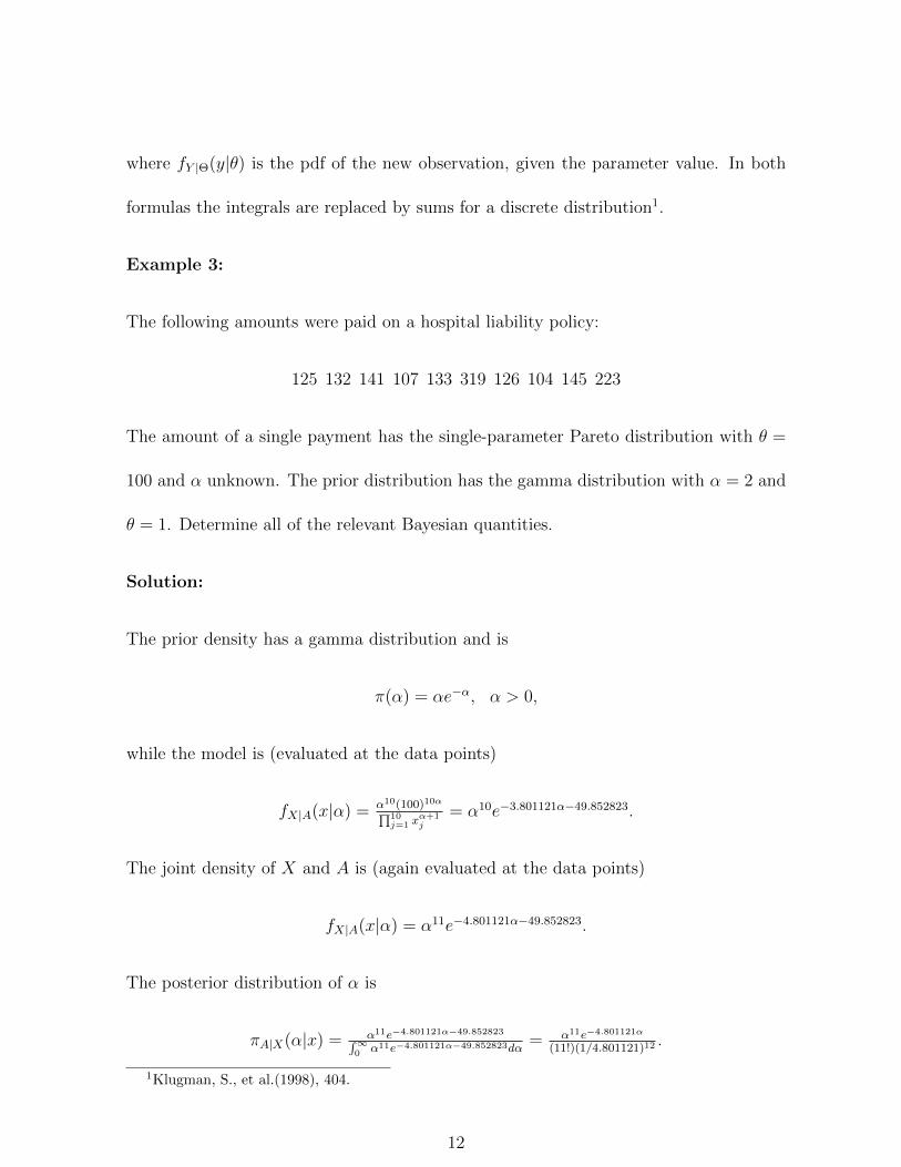
Example 3:
The following amounts were paid on a hospital liability policy:
125 132 141 107 133 319 126 104 145 223
The amount of a single payment has the single-parameter Pareto distribution with θ =
100 and α unknown. The prior distribution has the gamma distribution with α = 2 and
θ = 1. Determine all of the relevant Bayesian quantities.
Solution:
The prior density has a gamma distribution and is
π(α) = αe−α, α > 0,
while the model is (evaluated at the data points)
fX|A(x|α) = α10(100)10α∏10j=1 x
α+1j
= α10e−3.801121α−49.852823.
The joint density of X and A is (again evaluated at the data points)
fX|A(x|α) = α11e−4.801121α−49.852823.
The posterior distribution of α is
πA|X(α|x) = α11e−4.801121α−49.852823∫∞0 α11e−4.801121α−49.852823dα
= α11e−4.801121α
(11!)(1/4.801121)12 .
1Klugman, S., et al.(1998), 404.
12
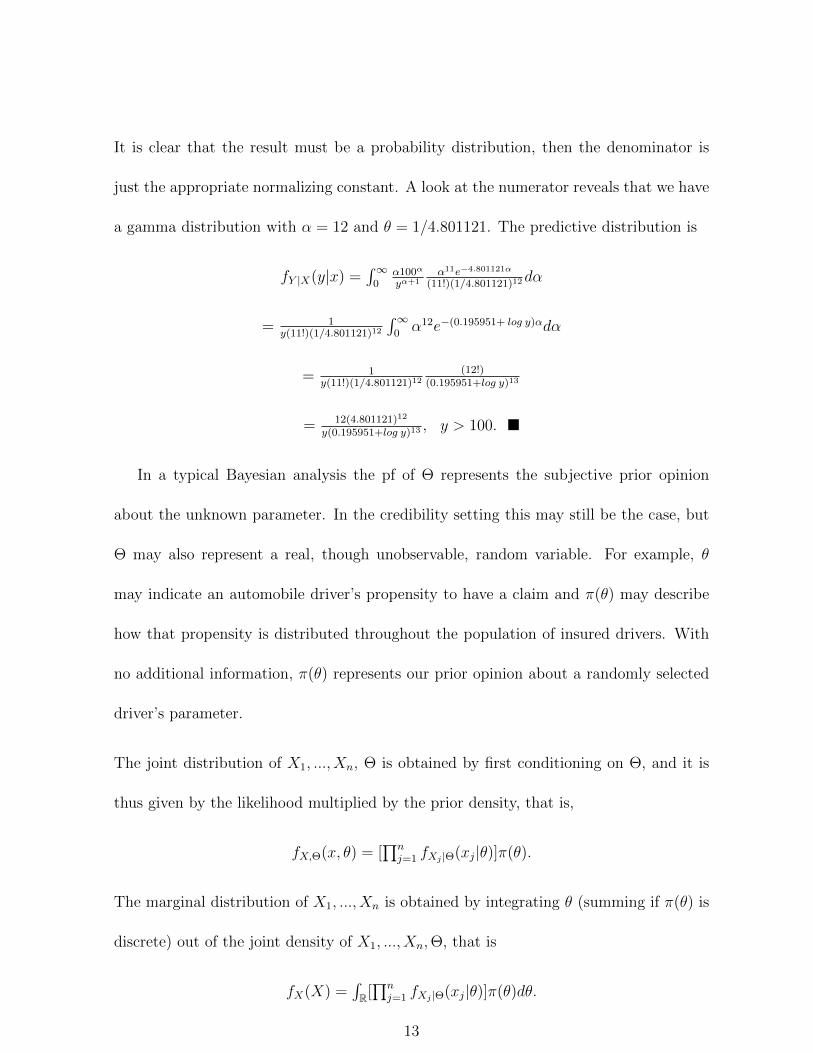
It is clear that the result must be a probability distribution, then the denominator is
just the appropriate normalizing constant. A look at the numerator reveals that we have
a gamma distribution with α = 12 and θ = 1/4.801121. The predictive distribution is
fY |X(y|x) =∫∞
0α100α
yα+1α11e−4.801121α
(11!)(1/4.801121)12dα
= 1y(11!)(1/4.801121)12
∫∞0α12e−(0.195951+ log y)αdα
= 1y(11!)(1/4.801121)12
(12!)(0.195951+log y)13
= 12(4.801121)12
y(0.195951+log y)13 , y > 100. �
In a typical Bayesian analysis the pf of Θ represents the subjective prior opinion
about the unknown parameter. In the credibility setting this may still be the case, but
Θ may also represent a real, though unobservable, random variable. For example, θ
may indicate an automobile driver’s propensity to have a claim and π(θ) may describe
how that propensity is distributed throughout the population of insured drivers. With
no additional information, π(θ) represents our prior opinion about a randomly selected
driver’s parameter.
The joint distribution of X1, ..., Xn, Θ is obtained by first conditioning on Θ, and it is
thus given by the likelihood multiplied by the prior density, that is,
fX,Θ(x, θ) = [∏n
j=1 fXj |Θ(xj|θ)]π(θ).
The marginal distribution of X1, ..., Xn is obtained by integrating θ (summing if π(θ) is
discrete) out of the joint density of X1, ..., Xn,Θ, that is
fX(X) =∫R[∏n
j=1 fXj |Θ(xj|θ)]π(θ)dθ.
13

The information about Θ “posterior” to the observation of X = (X1, ..., Xn)′
is summa-
rized in the posterior distribution of Θ. This is simply the conditional density of Θ given
that X equals x = (x1, ..., xn)′, which we express notationally as Θ|X = x or simply as
Θ|X or Θ|x, and this is also the ratio of the joint density of X1, ..., Xn,Θ to the marginal
density of X1, ..., Xn. In other words, the posterior density is
πΘ|X(θ|x) =[∏nj=1 fXj |Θ(xj |θ)]π(θ)∫
R[∏nj=1 fXj |Θ(xj |θ)]π(θ)dθ
.
From a practical viewpoint, the denominator does not depend on θ and simply serves as
a normalizing constant. Thus, as a function of θ, πΘ|X(θ|x) is proportional to
[∏n
j=1 fXj |Θ(xj|θ)]π(θ)
and if the form of the terms involving θ is recognized as belonging to a particular dis-
tribution, then it is not necessary to evaluate the denominator, but only to identify the
appropriate normalizing constant. A point estimate of θ derived from πΘ|X(θ|x) requires
the selection of a loss function, and the choice of squared error loss results in the posterior
mean:
E(Θ|X = x) =∫R θπΘ|X(θ|x)dθ.
3.2 Derivation of the Bayesian Credibility Model
The framework that will be employed to develop the credibility models in this Thesis
will be Bayesian. Hence, it will be assumed that there exists some prior opinion regarding
the risk characteristics of the population, which will be described via the random variable
Θ. The prior probability density function will be denoted as πΘ(θ), a function with one
14
parameter, θ. Also, it will be assumed that Xi|θ and Xj|θ are independent and identically
distributed ∀ i 6= j, where in the present context the subscript designates duration. Other
preliminary Bayesian relationships that are needed are given as follows:
• X will represent a vector of either loss amounts or claim frequencies
• The conditional distribution of X given Θ = θ is defined as,
fX|Θ(x|θ) = f(x1, x2, ..., xn|θ) =∏n
i fXi|Θ(xi|θ)
• The joint pdf of X and Θ is : fX,Θ(x, θ)= fX|Θ(x|θ) · π(θ)
• The marginal distribution of X is: fX(x) =∫R fX,Θ(x, θ)dθ
• The posterior distribution of Θ|X is πΘ|X(θ|x) =fX,Θ(x,θ)
fX(x)
The significance of the posterior distribution is that it updates the a priori probability
statements regarding Θ, based on the observed values (x1, x2, ..., xn). From this, a revised
predictive distribution can be constructed that incorporates the observed xi values. The
predictive distribution is derived as follows. First, let Xn+1 denote the losses in the
upcoming year, (n + 1), which have not yet been observed. Also, let the expected
value of losses for year i given Θ be expressed as E(Xi|Θ) = µi(Θ). In particular,
E(Xn+1|Θ) = µn+1(Θ), where µn+1(Θ) represents the hypothetical mean for next year.
Now, the conditional distribution of Xn+1 given X = [x1, x2, ..., xn] may be expressed as,
fXn+1|X(xn+1|x) = f(x1,...,xn,xn+1)f(x1,...,xn)
= f(x1,...,xn,xn+1)fX(x)
.
Furthermore,
[∏n+1i fXi|Θ(xi|θ)
]π(θ) = fXn+1|Θ(xn+1|θ) ·
[∏ni fXi|Θ(xi|θ)
]π(θ)
15

= fXn+1|Θ(xn+1|θ) · πΘ|X(θ|x) · fX(x).
Then,
f(x1, ..., xn, xn+1) =∫R
[∏n+1i fXi|Θ(xi|θ)
]π(θ)dθ =
∫R fXn+1|Θ(xn+1|θ)·πΘ|X(θ|x)·fX(x)dθ.
Finally, we can express the predictive distribution as,
fXn+1|X(xn+1|x) =∫R fXn+1|Θ(xn+1|θ) · πΘ|X(θ|x) · fX(x)dθ / f(x1, ..., xn) , or,
fXn+1|X(xn+1|x) =∫R fXn+1|Θ(xn+1|θ) · πΘ|X(θ|x)dθ.
Then, the Bayesian Premium (or the expected value of the predictive distribution, a
posteriori) may be obtained as follows:
E[Xn+1|X = x] =∫R xn+1fXn+1|X(xn+1|x)dxn+1
=∫R xn+1[
∫fXn+1|Θ(xn+1|θ) · πΘ|X(θ|x)dθ]dxn+1
=∫R[∫xn+1fXn+1|Θ(xn+1|θ)dxn+1]πΘ|X(θ|x)dθ
=∫R µn+1(Θ) · πΘ|X(θ|x)dθ
=∑
Θ µn+1(Θ) · πΘ|X(θ|x), in the discrete case.
Thus, the Bayesian Premium is the integral (or summation in the discrete setting)
over Θ of the hypothetical mean, µn+1(Θ), multiplied by the posterior density function,
πΘ|X(θ|x). Computationally, this last expression is generally much easier to implement
than using the distribution of fXn+1|X(xn+1|x) directly.
16

Example 4:
In this random experiment, there is a big bowl and two boxes (Box 1 and Box 2).
The bowl consists of a large quantity of balls, 80% of which are white and 20% of which
are red. In Box 1, 60% of the balls are labeled 0, 30% are labeled 1 and 10% are labeled
2. In Box 2, 15% of the balls are labeled 0, 35% are labeled 1 and 50% are labeled 2. In
the experiment, a ball is selected at random from a bowl. The color of the selected ball
from the bowl determines which box to use (if the ball is white, then use Box 1, if red,
use Box 2). Then balls are drawn at random from the selected box (Box i) repeatedly
with replacement and the values of the series of selected balls are recorded. The value
of the first selected ball is X1, the value of the second selected ball is X2, and so on.
Suppose that a random person performs this random experiment (we do not know
whether he uses Box 1 or Box 2) and that his first ball is a 1 (X1 = 1) and his second
ball is a 2 (X2 = 2). What is the predicted value X3 of the third selected ball?
Solution:
For convenience, we will denote “draw of a white ball from bowl” by θ = 1 and “draw of a
red ball from bowl” by θ = 2. Box 1 and Box 2 represent conditional distributions. Bowl
is a distribution for the parameter θ. The distribution given the bowl is a probability
distribution over the space of all parameter values (the prior distribution). The prior
distribution of θ and the conditional distributions of X given θ are restated as follows:
πθ(1) = 0.8, πθ(2) = 0.2
fX|Θ(0|θ = 1) = 0.60, fX|Θ(1|θ = 1) = 0.30, fX|Θ(2|θ = 1) = 0.10
17

fX|Θ(0|θ = 2) = 0.15, fX|Θ(1|θ = 2) = 0.35, fX|Θ(2|θ = 2) = 0.50.
The following shows the conditional means E[X|θ] and the unconditional mean E[X]:
E[X|θ = 1] = 0.6(0) + 0.3(1) + 0.1(2) = 0.50,
E[X|θ = 2] = 0.15(0) + 0.35(1) + 0.5(2) = 1.35,
E[X] = 0.8(0.50) + 0.2(1.35) = 0.67.
The Unconditional Distributions:
fX(0) = 0.6(0.8) + 0.15(0.2) = 0.51,
fX(1) = 0.3(0.8) + 0.35(0.2) = 0.31,
fX(2) = 0.1(0.8) + 0.50(0.2) = 0.18.
The Marginal Probabilities:
fX1,X2(1, 2) = 0.1(0.3)(0.8) + 0.5(0.35)(0.2) = 0.059.
The Posterior Distributions of θ:
πΘ|X1,X2(1|1, 2) = 0.1(0.3)(0.8)0.059
= 2459,
πΘ|X1,X2(2|1, 2) = 0.5(0.35)(0.2)0.059
= 3559.
The Predictive Distributions of X:
fX3|X1,X2(0|1, 2) = 0.62459
+ 0.153559
= 19.6559,
fX3|X1,X2(1|1, 2) = 0.32459
+ 0.353559
= 19.4559,
18

fX3|X1,X2(2|1, 2) = 0.12459
+ 0.503559
= 19.9059.
The posterior distribution πθ(·|1, 2) is the conditional probability distribution of the
parameter θ given the observed data X1 = 1 and X2 = 2. This is a result of applying
Bayes theorem. The predictive distribution fX3|X1,X2(·|1, 2) is the conditional probability
distribution of a new observation given the past observed data of X1 = 1 and X2 = 2.
Since both of these distributions incorporate the past observations, the Bayesian estimate
of the next observation is the mean of the predictive distribution.
E[X3|X1 = 1, X2 = 2] = 0fX3|X1,X2(0|1, 2) + 1fX3|X1,X2(1|1, 2) + 2fX3|X1,X2(2|1, 2)
= 019.6559
+ 119.4559
+ 219.9059
= 59.2559
= 1.0042372,
E[X3|X1 = 1, X2 = 2] = E[X|θ = 1]πΘ|X1,X2(1|1, 2) + E[X|θ = 2]πΘ|X1,X2(2|1, 2)
= 0.52459
+ 1.353559
= 59.2559
= 1.0042372. �
3.3 Conjugate Priors in Bayesian Credibility
One very nice property for some combinations of distributions is that the past experience,
X, produces a posterior distribution that is the same distribution as the original prior,
but the parameters have been updated based on the experience, X. Priors that behave
this way are called conjugate priors, when combined with an appropriate distribution
that follows this property. One of the most important conjugate priors is the Normal-
Normal case, and we will consider this case in more details in this section.
Assume that Xi|Θ ∼ N(θ, v), and Θ ∼ N(µ, a). Then, the posterior distribution is
19
πΘ|X(θ|x) = f(x,θ)fX(x)
∝ (2πv)−n2 exp[− 1
2v(xi − θ)2](2πa)−
n2 exp[− 1
2a(θ − µ)2]
∝ exp[− 12v
∑i(xi − θ)2 − 1
2a(θ − µ)2]
= exp[− 12v
(∑
i x2i − 2θ
∑i xi + nθ2)− 1
2a(θ − µ)2]
∝ exp[− 12v
(−2θnx+ nθ2)− 12a
(θ − µ)2]
= exp[ θnxv− nθ2
2v− θ2
2a+ θµ
a]
= exp[(− n2v− 1
2a)θ2 + (nx
v+ µ
a)θ].
Now, define µ∗ = [nxv
+ µa]a∗, and let a∗ = [n
v+ 1
a]−1. Then, substitution into the previous
expression yields,
= exp[−12(nv
+ 1a)θ2 + (µ∗
a∗)θ]
∝ exp[− 12a∗θ2 + µ∗
a∗θ − µ2
∗2a∗
]
= exp[− 12a∗
(θ2 − 2µ∗θ + µ2∗)]
= exp[− 12a∗
(θ − µ∗)2],
which shows that the posterior distribution πΘ|X(θ|x) ∼ N(µ∗, a∗).
The mean of the predictive distribution is,
E[Xn+1|X = x] =∫R µn+1(Θ) · πΘ|X(θ|x)dθ =
∫R θ · πΘ|X(θ|x)dθ,
since Xi|Θ ∼ N(θ, v), and thus E(Xi|Θ) = θ. But this expression is simply the formula
for the first raw moment (i.e. the expected value) of the posterior distribution, which
was already shown to equal µ∗. Thus, the Bayesian Premium in the normal conjugate
20

prior case is µ∗. However, it is instructive to rearrange the expression for µ∗ in a manner
that is more revealing:
µ∗ = [nxv
+ µa][nv
+ 1a]−1 = [nx
v+ µ
a][ avna+v
] = (nv)( avna+v
)x+ ( 1a)( avna+v
)µ
= ( nana+v
)x+ ( vna+v
)µ = ( nn+ v
a)x+ (
va
n+ va)µ.
If we let va
= k, then the Bayesian Premium for the Normal-Normal case can be written
as,
µ∗ = E[Xn+1] = (n
n+ k)x+ (
k
n+ k)µ,
where n is the sample size, and k is the ratio of the within variance to the between
variance.
21

Chapter 4
The Buhlmann Credibility Model
4.1 Target Shooting Example
In the classic paper by Stephen Philbrick1 there is an excellent target shooting example
that illustrates the ideas of Buhlmann Credibility. Assume there are four marksmen
each shooting at his own target. Each marksmans shots are assumed to be distributed
around his target, marked by one of the letters A, B, C, and D, with an expected mean
equal to the location of his target. Each marksman is shooting at a different target.
If the targets are arranged as in Figure 1, the resulting shots of each marksman
would tend to cluster around his own target. The shots of each marksman have been
distinguished by a different symbol. So for example the shots of marksman B are shown
as triangles. We see that in some cases one would have a hard time deciding which
marksman had made a particular shot if we did not have the convenient labels.
The point E represents the average of the four targets A, B, C, and D. Thus E is the
grand mean. If we did not know which marksman was shooting we would estimate that
the shot would be at E; the a priori estimate is E.
1Philbrick, S. (1981).
22

Once we observe a shot from an unknown marksman, we could be asked to estimate
the location of the next shot from the same marksman. Using Buhlmann Credibility our
estimate would be between the observation and the a priori mean of E. The larger the
credibility assigned to the observation, the closer the estimate is to the observation. The
smaller the credibility assigned to the data, the closer the estimate is to E.
Figure 4.1: Target Shooting Figure 1
There are a number of features of this target shooting example that control how
much Buhlmann Credibility is assigned to our observation. We have assumed that the
marksmen are not perfect; they do not always hit their target. The amount of spread of
their shots around their targets can be measured by the variance. The average spread
over the marksmen is the Expected Value of the Process Variance (EPV). The better
the marksmen, the smaller the EPV and the more tightly clustered around the targets
23

the shots will be.
The worse the marksmen, the larger the EPV and the less tightly the shots are
spread. The better the marksmen, the more information contained in a shot. The worse
the marksmen, the more random noise contained in the observation of the location
of a shot. Thus when the marksmen are good, we expect to give more weight to an
observation (all other things being equal) than when the marksmen are bad. Thus the
better the marksmen, the higher the credibility.
Figure 4.2: Target Shooting Figure 2
The smaller the Expected Value of the Process Variance the larger the credibility.
This is illustrated by Figure 2. It is assumed in Figure 2 that each marksman is better
than was the case in Figure 1. The EPV is smaller and we assign more credibility to the
observation. This makes sense, since in Figure 2 it is a lot easier to tell which marksman
is likely to have made a particular shot based solely on its location.
24

Another feature that determines how much credibility to give an observation is how
far apart the four targets are placed. As we move the targets further apart (all other
things being equal) it is easier to distinguish the shots of the different marksmen. Each
target is a hypothetical mean of one of the marksmens shots. The spread of the targets
can be quantified as the Variance of the Hypothetical Means.
Figure 4.3: Target Shooting Figure 3
As illustrated in Figure 3, the further apart the targets the more credibility we would
assign to our observation. The larger the VHM the larger the credibility. It is easier to
distinguish which marksman made a shot based solely on its location in Figure 3 than
25
in Figure 1.
The third feature that one can vary is the number of shots observed from the same
unknown marksman. The more shots we observe, the more information we have and
thus the more credibility we would assign to the average of the observations.
Each of the three features discussed is reflected in the formula for Buhlmann Credi-
bility
Z = NN+K
= N(V HM)N(V HM)+EPV
Thus, as the EPV increases, Z decreases; as V HM increases, Z increases; and as N
increases, Z increases.
There are two separate reasons why the observed shots vary. First, the marksmen
are not perfect. In other words the Expected Value of the Process Variance is positive.
Even if all the targets were in the same place, there would still be a variance in the
observed results. This component of the total variance due to the imperfection of the
marksmen is quantified by the EPV.
Second, the targets are spread apart. In other words, the Variance of the Hypothetical
Means is positive. Even if every marksman were perfect, there would still be a variance
in the observed results, when the marksmen shoot at different targets. This component
of the total variance due to the spread of the targets is quantified by the VHM.
One needs to understand the distinction between these two sources of variance in the
observed results. Also one has to know that the total variance of the observed shots is
26

a sum of these two components: Total V ariance = EPV + V HM .
4.2 Credibility Parameters
Intuition says that two factors appear important in finding the right balance between
class rating and individual risk experience rating:How homogeneous are the classes? If
all of the risks in a class are identical and have the same expected value for losses, then
why bother with individual experience rating? Just use the class rate. On the other
hand, if there is significant variation in the expected outcomes for risks in the class, then
relatively more weight should be given to individual risk loss experience.
Each risk in the class has its own individual risk mean called its hypothetical mean.
The Variance of the Hypothetical Means (VHM) across risks in the class is a statistical
measure for the homogeneity or vice versa, heterogeneity, within the class. A smaller
VHM indicates more class homogeneity and, consequently, argues for more weight going
to the class rate. A larger VHM indicates more class heterogeneity and, consequently,
argues for less weight going to the class rate.
How much variation is there in an individual risks loss experience? If there is a large
amount of variation expected in the actual loss experience for an individual risk, then
the actual experience observed may be far from its expected value and not very useful
for estimating the expected value. In this case, less weight, i.e., less credibility, should
be assigned to individual experience. The process variance, which is the variance of the
risks random experience about its expected value, is a measure of the variability in an
27

individual risks loss experience. The Expected Value of the Process Variance (EPV) is
the average value of the process variance over the entire class of risks.
Let Xi represent the sample mean of n observations for a randomly selected riski.
Because there are n observations, the variance in the sample mean Xi is the variance in
one observation for the risk divided by n. Given risk i, this variance is PVi where PV is
the process variance of one observation. Because risk i was selected at random from the
class of risks, an estimator for its variance is E[PVi/n] = E[PVi]/n − EPV/n. This is
the Expected Value of the Process Variance for risks in the class divided by the number
of observations made about the selected risk. It measures the variability expected in an
individual risks loss experience.
Letting µ represent the overall class mean, a risk selected at random from the class
will have an expected value equal to the class mean µ. The variance of the individual
risk means about µ is the VHM, the Variance of the Hypothetical Means. There are
two estimators for the expected value of the ith risk: (1) the risks sample mean Xi, and
(2) the class mean µ. How should these two estimators be weighted together? A linear
estimate with the weights summing to 1.00 would be:
Estimate = wXi + (1− w)µ.
An optimal method for weighting two estimators is to choose weights proportional
to the reciprocals of their respective variances. This results in giving more weight to the
estimator with smaller variance and less weight to the estimator with larger variance. In
many situations this will result in a minimum variance estimator. The resulting weights
28

are:
w =1
EPV/n1
EPV/n+ 1VHM
and
(1− w) = w =1
VHM1
EPV/n+ 1VHM
Thus,
w = nn+ EPV
VHM
and (1− w) = 1− nn+ EPV
VHM
.
Setting K = EPV/V HM , the weight assigned to the risks observed mean is
w = nn+K
.
The actual observation during time t for that particular risk or group will be denoted
by xt, which will be the observation of corresponding random variable Xt, where t is an
integer. For example, Xt may represent the following:
• Number of claims in period t;
• Loss ratio in year t;
• Loss per exposure in year t.
An individual risk is a member of a larger population and the risk has an associated
risk parameter Θ that distinguishes the individuals risk characteristics. It is assumed
that the risk parameter is distributed randomly through the population and Θ will denote
29

the random variable. The distribution of the random variable Xt depends upon the value
of Θ: fx|Θ(xt|Θ). For example, Θ may be a parameter in the distribution function of Xt.
If Xt is a continuous random variable, the mean for Xt given Θ = θ, is the conditional
expectation, EX|Θ[Xt|Θ = θ] =∫xtfX|Θ(xt|θ)dxt = µ(θ), where the integration is over
the support of fX|Θ(xt|θ). If Xt is a discrete random variable, then a summation should
be used:
EX|Θ[Xt|Θ = θ] =∑
allxtxtfX|Θ(xt|θ).
The risk parameter represented by the random variable Θ has its own probability
density function (pdf): fΘ(θ). The pdf for Θ describes how the risk characteristics are
distributed within the population. If two risks have the same parameter θ, then they are
assumed to have the same risk characteristics including the same mean µ(θ).
The unconditional expectation of Xt is:
E[Xt] =∫∫
R xtfX,Θ(xt, θ)dxtdθ =∫∫
R xtfX,Θ(xt, θ)fΘ(θ)dxtdθ =
∫R
[∫xtfX,Θ(xt, θ)dxt
]fΘ(θ)dθ = EΘ[EX|Θ[Xt|Θ]] = EΘ[µ(θ)] = µ.
The conditional variance of Xt given Θ = θ is
V arX|Θ[Xt|Θ = θ] = EX|Θ[(Xt − µ(θ))2|Θ = θ] =∫∫
R(Xt − µ(θ))2fX|Θ(xt|θ)dxt = σ2(θ).
This variance is also called the process variance for the selected risk. The unconditional
variance of Xt, also referred to as the total variance, is given by the Total Variance
formula:
30

V ar[Xt] = V arΘ[EX|Θ[Xt|Θ]] + EΘ[V arX|Θ[Xt|Θ]].
4.3 Derivation of the Buhlmann Credibility Model
The Buhlmann model assumes that for any selected risk, the random variables
{X1, X2, ..., Xn, Xn+1, ...} are independently and identically distributed. For the se-
lected risk, each Xt has the same probability distribution for any time period t, both
for the X1, X2, .., Xn random variables in the experience period, and future outcomes
Xn+1, Xn+2, .... As Hans Buhlmann described it, homogeneity in time is assumed.
The characteristics that determine the risks exposure to loss are assumed to be un-
changing and the risk parameter θ associated with the risk is constant through time for
the risk. The means and variances of the random variables for the different time periods
are equal and are labeled µ(θ) and σ2(θ), respectively.
Hypothetical Mean: µ(θ) = EX|Θ[X1|θ] = ... = EX|Θ[XN |θ] = EX|Θ[XN+1|θ].
Process Variance: σ2(θ) = V arX|Θ[X1|θ] = ... = V arX|Θ[XN |θ] = V arX|Θ[XN+1|θ].
The hypothetical means and process variances will vary among risks, but they are as-
sumed to be unchanging for any individual risk in the Buhlmann model. To apply
Buhlmann credibility, the average values of these quantities over the whole population
of risks are needed, along with the variance of the hypothetical means for the population:
1. Population Mean: µ = EΘ[µ(Θ)] = EΘ[EX|Θ[Xt|Θ]]
2. Expected Value of Process Variance: EPV = EΘ[σ2(Θ)] = EΘ[V arX|Θ[X|Θ]]
31
3. Variance of Hypothetical Means: V HM = V arΘ[µ(Θ)] = EΘ[(µ(Θ)− µ)2]
The population mean µ = EΘ[EX|Θ[Xt|Θ]] provides an estimate for the expected value
of Xt in the absence of any prior information about the risk. The EPV indicates the
variability to be expected from observations made about individual risks. The VHM is
a measure of the differences in the means among risks in the population.
Because µ(Θ) is unknown for the selected risk, the mean X = ( 1N
)∑N
t=1Xt, is used
in the estimation process. It is an unbiased estimator for µ(θ),
EX|Θ[X|θ] = EX|Θ[( 1N
)∑N
t=1Xt|θ] = ( 1N
)∑N
t=1 EX|Θ[Xt|θ] = ( 1N
)∑N
t=1 µ(θ) = µ(θ).
The conditional variance of X, assuming independence of the Xt given θ, is
V arX|Θ[X|θ] = V arX|Θ[( 1N
)∑N
t=1Xt|θ] =
( 1N
)2∑N
t=1 V arX|Θ[Xt|θ] = ( 1N
2)∑N
t=1 σ2(θ) = σ2(θ)
N.
The unconditional variance of X is
V ar[X] = V arΘ[EX|Θ[X|Θ]] + EΘ[V arX|Θ[X|Θ]] =
V arΘ[µ(Θ)] + EΘ[σ2(Θ)]N
= V HM + EPVN
The Buhlmann credibility assigned to estimator X is given by the well-known formula
Z = NN+K
,
where N is the number of observations for the risk and K = EPV/V HM . Multiplying
the numerator and denominator by (V HM/N) gives an alternative form:
32

Z = V HMVHM+EPV
N
.
Therefore Z = NN+K
, can be written as
Z = V arΘ[µ(Θ)]
V ar[X].
The numerator is a measure of how far apart the means of the risks in the population
are, while the denominator is a measure of the total variance of the estimator. The
credibility weighted estimate for
µ(θ) = EX|Θ[Xt|θ], for t = 1, 2, ..., N,N + 1, ...,
µ(θ) = Z · X + (1− Z) · µ.
The estimator µ(θ) is a linear least squares estimator for µ(θ). This means that
E[[Z · X + (1− Z) · µ]− µ(Θ)2] is minimized when Z = N/(N +K).
Continuing Example 4:
Suppose that random person performs this random experiment (we do not know
whether he uses Box 1 or Box 2) and that his first ball is a 1 (X1 = 1) and his second
ball is a 2 (X2 = 2). What is the predicted value X3 of the third selected ball?
Solution:
The following restates the prior distribution of Θ and the conditional distribution of
X|Θ. We denote “white ball from the bowl” by Θ = 1 and “red ball from the bowl” by
Θ = 2.
πθ(1) = 0.8, πθ(2) = 0.2
33

fX|Θ(0|θ = 1) = 0.60, fX|Θ(1|θ = 1) = 0.30,
fX|Θ(2|θ = 1) = 0.10,
fX|Θ(0|θ = 2) = 0.15, fX|Θ(1|θ = 2) = 0.35,
fX|Θ(2|θ = 2) = 0.50.
The following computes the conditional means (hypothetical means) and conditional
variances (process variances) and the other parameters of the Buhlmann method.
Hypothetical Means:
E[X|Θ = 1] = 0.60(0) + 0.30(1) + 0.10(2) = 0.50,
E[X|Θ = 2] = 0.15(0) + 0.35(1) + 0.50(2) = 1.35,
E[X2|Θ = 1] = 0.60(0) + 0.30(1) + 0.10(4) = 0.70,
E[X2|Θ = 2] = 0.15(0) + 0.35(1) + 0.50(4) = 2.35.
Process Variances:
V ar[X|Θ = 1] = 0.70− 0.502 = 0.45,
V ar[X|Θ = 2] = 2.35− 1.352 = 0.5275.
Expected Value of the Hypothetical Means:
µ = E[X] = E[E[X|Θ]] = 0.80(0.50) + 0.20(1.35) = 0.67.
Expected Value of the Process Variance:
EPV = E[V ar[X|Θ]] = 0.8(0.45) + 0.20(0.5275) = 0.4655.
34

Variance of the Hypothetical Means:
V HM = V ar[E[X|Θ]] = 0.80(0.50)2 + 0.20(1.35)2 − 0.672 = 0.1156
Buhlmann Credibility Factor:
K = 46551156
,
Z = 22+ 4655
1156
= 23126967
= 0.33185.
Buhlmann Credibility Estimate:
C = 23126967
32
+ 46556967
(0.67) = 6586.856967
= 0.9454356. �
35

Chapter 5
The Buhlmann - Straub CredibilityModel
5.1 Credibility Parameters
The requirement that the random variables X1, X2, ..., XN , XN+1... for a risk be iden-
tically distributed is easily violated in the real world. For example:
• The work force of a workers compensation policyholder may change in size from
one year to the next.
• The number of vehicles owned by a commercial automobile policyholder may
change through time.
• The amount of earned premium for a rating class varies from year to year.
In all of these cases, one should not assume that variables X1, X2, ..., XN , XN+1... are
identically distributed, although an assumption of independence may be warranted. A
risks exposure to loss may vary and it is assumed that this exposure can be measured.
Some measures of exposure to loss are:
• Amount of insurance premium
36

• Number of employees
• Payroll
• Number of claims
The Buhlmann-Straub model assumes that the means of the random variables are equal
for the selected risk, but that the process variances are inversely proportional to the
size of the risk during each observation period. For example, when the risk is twice as
large, the process variance is halved. For the Buhlmann-Straub model occurs following
assuptions:
Hypothetical Mean for Risk θ per Unit of Exposure: µ(θ) = EX|Θ[XN |θ].
Process Variance for Risk θ: V arX|θ[XN |θ] = σ2(θ)mN
.
The random variables Xt represent number of claims, monetary losses, or some other
quantity of interest per unit of exposure, and mt is the measure of exposure.
How should random variables X1, X2, ..., XN , XN+1... associated with a selected risk
(or group of risks) be combined to estimate the hypothetical mean µ(θ)? A weighted
average using the exposures mt will give a linear estimator for µ(θ) with minimum
variance:
µ =∑N
t=1mt.
The weighted average is
X =∑N
t=1(mtm
)Xt.
37

Recall that the variance of each Xt given θ is σ2(θ)/mt. For a weighted average X =∑Nt=1 wtXt, the variance of X will be minimized by choosing the weights wt to be inversely
proportional to the variances of the each individual Xt. That is, random variables with
smaller variances should be given more weight. So, the following weights wt = mt/m are
called for under the current assumptions.
The conditional expected value and variance of X given risk parameter θ are
EX|Θ[X|θ] = EX|Θ[∑N
t=1mtmXt|θ] =
∑Nt=1
mtmEX|Θ[Xt|θ] =
∑Nt=1
mtmµ(θ) = µ(θ),
V arX|Θ[X|θ] = V arX|Θ[∑N
t=1mtmXt|θ] =
∑Nt=1
mtmV arX|Θ[Xt|θ] =
∑Nt=1
mtm
(σ2(θ)mt
) = σ2(θ)m.
The EPV and VHM are defined to be EPV = Eθ[σ2(Θ)] and V HM = V arθ[µ(Θ)] where
the expected value is over all risk parameters in the population. The loss per unit of
exposure is used because the exposure can vary through time and from risk to risk. The
unconditional mean and variance of X are
E[X] = EΘ[EX|Θ[X|Θ]] = EΘ[µ(Θ)] = µ,
V ar[X] = V arΘ[EX|Θ[X|Θ]] + EΘ[V arX|Θ[X|Θ]]] =
V arΘ[µ(Θ)] + EΘ[σ2(Θ)]m
= V HM + EPVm.
The credibility assigned to the estimator X of µ(θ) is
Z = V HMVHM+EPV
m
⇒ Z = mm+K
.
The total exposure m replaces N in the Buhlmann formula and the parameter K is
defined as usual:
38

K = EPVV HM
= EΘ[σ2(Θ)]V arΘ[µ(Θ)]
The Buhlmann model is actually a special case of the more general Buhlmann-Straub
model with mt = 1 ∀t. The credibility weighted estimate is
µ(θ) = Z · X + (1− Z) · µ.
5.2 Nonparametric Estimation
In a nonparametric setup, no assumptions are made about the form or parameters
of the distributions of Xit, nor are any assumptions made about the distribution of the
risk parameters Θi. In the Buhlmann-Straub model, the Ni outcomes for risk i have the
same means but the process variances are inversely related to the exposure. The number
of observations Ni has a subscript indicating that the number of observations can vary
by risk in the Buhlmann-Straub model.
The Buhlmann-Straub Model is more complicated because a risks exposure to loss
can vary from year to year, and the number of years of observations can change from
risk to risk. The reason that Buhlmann-Straub can handle varying numbers of years is
because the number of years of data for a risk is reflected in the total exposure for the
risk. Estimators for risk mean and variance are the following:
X =∑R
i=1miXi/m and EPV =∑R
i=1(Ni − 1)σi2/(∑R
i=1(Ni − 1))
In the Buhlmann-Straub model, the mean is assumed to be constant through time for
each risk i:
39

µ(θi) = EX|θ[Xi1|θi] = EX|θ.
Also, Xi is an unbiased estimator for the mean of risk i:
EX|Θ[Xi|Θi] = EX|Θ[( 1mi
)∑Ni
i=1mitXit|θi] =
( 1mi
)∑Ni
i=1 mitEX|Θ[Xit|θi] = ( 1mi
)∑Ni
i=1mitµ(θi) = µ(θi).
The process variance of Xit is inversely proportional to the exposure:
V arX|θ[Xit|θi] = σ2(θi)/mit.
This means that for risk i,
σ2(θi) = mitEX|Θ[(Xit − µ(θi))2|θi], for t = 1 to Ni.
σ2(θi) = mitEX|Θ[(Xit − µ(θi))2|θ − i], for t = 1 to Ni.
Summing both sides over t and dividing by the number of terms Ni yields
( 1Ni
)∑Ni
i=1 σ2i (θi) = ( 1
Ni)∑Ni
i=1mitEX|Θ[(Xit − µ(θi))2|θ − i], or
σ2i (θi) = EX|Θ[( 1
Ni)∑Ni
i=1mit(Xit − µ(θi))2|θ − i].
The quantity µ(θi) is unknown, so Xi is used instead in the estimation process. This
reduces the degrees of freedom by one so Ni is replaced by Ni − 1 in the denominator:
σ2i (θi) = EX|Θ[( 1
Ni−1)∑Ni
i=1mit(Xit − Xi)2|θ − i].
Thus, an unbiased estimator for σ2i is
(σi)2 = ( 1
Ni−1)∑Ni
i=1 mit(Xit − Xi)2.
40
The EPV can be estimated by combining process variance estimates σi2 of the R risks.
If they are combined with weights wi = (Ni − 1)/(∑R
i=1(Ni − 1)), then an unbaised
estimator for the EPV is
ˆEPV =∑R
i=1wi(σi)2 =
∑Ri=1
∑Nit=1 mit(Xit−Xi)2∑Ri=1(Ni−1)
The hypothetical mean for risk i is µ(θi). The variance of the hypothetical means can
be written as
V HM = Eθ[(µ(Θi)− µ)2], where µ = Eθ[µ(Θi)].
Because the observed values of the random variables Xi and X are estimators for µ(θi)
and µ, respectively, a good starting point for developing an estimator for the variance
of the hypothetical means is: 1(R−1)
∑Ri=1 mi(Xi − X)2. Each term is weighted by its
total exposure over the experience period. However, this is not unbiased. An unbiased
estimator is
ˆV HM =(∑R
i=1mi(Xi − X)2 − (R− 1) ˆEPV)/(m−
(1m
)∑Ri=1 m
2i
).
With the Buhlmann-Straub model, the measure to use in the credibility formula is the
total exposure for risk i over the whole experience period. The formulas to compute
credibility weighted estimates are
K =ˆEPVˆV HM, Zi = mi
mi+K, and
µ(θi) = Zi · Xi + (1− Zi) · X.
41

Chapter 6
An Analysis of Colorado CancerDeath Rates
6.1 Introduction to the Cancer Data Set
The case study presented in this chapter will be based on Colorado Health Information
Dataset (CoHID), furnished by the Colorado Department of Public Health and Environ-
ment. Death data are compiled from information reported on the Certificate of Death.
Data items are presented as reported. Information on the certificate concerning time,
place, and cause of death is typically supplied by medical personnel or coroners. De-
mographic information, such as age, race/ethnicity, or occupation, is generally reported
on the certificate by funeral directors from information supplied by the available next of
kin. CoHID only reports data for Colorado resident deaths.
Colorado Health Information Dataset presents Cause of Death Classification and To-
tal Crude Death Rate, the number of deaths per a specified number of population (i.e.,
per 1,000 or 100,000). Crude rates are not adjusted for differences in demographic distri-
butions among populations, such as age distributions. This dataset contains information
on over 100 causes of death in Colorado from 1990 through the most recent year avail-
42

Table 6.1: Denver County Deaths by Cancer Data Set
Year Total Death Total Population Total Crude Death Rate per 100,0002000 909 556,738 163.32001 919 563,300 163.12002 947 559,090 169.42003 906 560,348 161.72004 914 560,230 163.12005 859 559,459 153.52006 828 562,862 147.12007 808 570,437 141.62008 858 581,903 147.42009 846 595,573 1422010 897 604,875 148.32011 870 620,917 140.12012 888 634,619 139.9Average 880.7 579,258 152
Table 6.2: Non-Denver Deaths by Cancer Data Set
Year Total Death Total Population Total Crude Death Rate per 100,0002000 4,987 3,782,063 131.82001 5,215 3,881,213 134.32002 5,425 3,945,619 137.52003 5,494 3,994,736 137.52004 5,271 4,048,581 130.12005 5,508 4,103,075 134.22006 5,695 4,182,798 136.12007 5,782 4,251,347 1362008 5,851 4,320,035 135.42009 6,092 4,381,280 1392010 6,132 4,445,108 137.92011 6,167 4,497,609 137.12012 6,426 4,554,064 141.1Average 5,695.7 4,183,656 136.1
43

able. The user is able to query death records for information such as: cause of death
by race/ethnicity, gender and age. The data can be extracted by zip code, county, or
region, allowing user also to analyze it geographically.
The death by cancer report from 2000 to 2012 (inclusive) is captured in Tables 6.1
and 6.2. Tables represent Denver County Dataset and Non-Denver (which is the rest of
Colorado State, excluding Denver). The first method to attempt is a Bayesian calculation
of the predictive distribution for the upcoming year, irrespective of class (i.e., µn+1(θ)).
Designating the Denver county as D, and the Non-Denver as N, we have xD = 152 and
xN = 136.14. Now, the prior probabilities are,
π(θD) = .121618362, π(θD) = .878381638.
However, the joint probabilities are now,
fX,ΘD(x, θD) = fX|Θ(x|θ) · π(θD) = 3.9031 · 10−16,
fX,ΘN (x, θN) = fX|Θ(x|θ) · π(θN) = 2.8912 · 10−15,
which, when summed, yield a marginal probability function, f(x) = 3.2824 · 10−15. This
implies that the posterior probabilities are,
πΘD|X(θD|x) =fX,ΘD (x,θD)
fX(x)= .118909024
πΘN |X(θN |x) =fX,ΘN (x,θN )
fX(x)= .881090976
Thus, the Bayesian estimate for the average of the Crude Death Rate for an upcoming
year is:
44

E(Xn+1|x) =∑
Θ µn+1(Θ) · πΘ|X(θ|x) = 155.98
for Denver county and
E(Xn+1|x) =∑
Θ µn+1(Θ) · πΘ|X(θ|x) = 132.7
for Non-Denver.
Now we will illustrate the Buhlmann credibility method. An unbiased estimator of
µ is µ = X = 144.1922071. Hence, an unbiased estimator of υ is
υ = 1r
∑ri=1 υi = 1
r(n−1)
∑ri=1
∑nj=1(Xij − Xi)
2 = 54.94614462.
Since we already have an unbiased estimator of υ given above, an unbiased estimator of
a is given by
a = 1r−n
∑ri=1(Xi − X)2 − υ
n= 128.7470678.
Then, k = υ/a = 0.426775891. The estimated credibility factor is Z = 0.968214567.
The estimated credibility premiums (or the crude death rates) are 152.08, for Denver
County and 136.29, for Non-Denver.
The next method to employ is the Buhlmann-Straub credibility model. It is a more
general Buhlmann setup, with E(Xij) = E[E(Xij|Θi)] = E[µ(Θi)] = µ(Θi). The credi-
bility parameters can be calculated as follows: XD = 152.0380657, XN = 136.1433452.
The overall mean is µ = X = 138.0764351.
Now, we obtain an unbiased estimator of υ, namely,
υ =∑ri=1
∑nij=1mij(Xij−Xi)
2∑ri=1(ni−1)
= 91825379.36.
45

Table 6.3: Table of Results for Denver County
Method Denver County (Crude Death Rate per 100,000)Buhlmann-Straub Credibility Premium 150.744µ(weighted) 143.760Buhlmann-Straub(weighted) 151.271Buhlmann Credibility Premium 152.087Posterior probabilities π(θ) 0.118909024Bayesian Credibility Premium 155.980
An unbiased estimator for a may be obtained by replacing υ by an unbiased estimator
υ and solving for a. That is, an unbiased estimator of a is
a = (m−m−1∑r
i=1m2i )−1[∑r
i=1mi(Xi − X)2 − υ(r − 1)]
= 119.3798741.
Then, k = υ/a = 769186.4316. The estimated credibility factors are ZD = 0.907321771
and ZN = 0.986054528. The estimated credibility premiums (or the crude death rates)
are 150.74, for Denver County and 136.17, for Non-Denver.
For the alternative estimator we would use
µ =∑ri=1 ZiXi∑ri=1 Zi
= 143.7602283
The credibility premiums are 151.27 for Denver County and 136.24 for Non-Denver.
Table 6.3 captures the results of finding the Crude Death Rate for Denver and Non-
Denver Countys using credibility methods. Table 6.5 captures the results of finding the
Crude Death Rate for Denver County for particular year, using the information in the
data set, excluding the predicted year.
46

Table 6.4: Table of Results for Non-Denver
Method Non-Denver County (Crude Death Rate per 100,000Buhlmann-Straub Credibility Premium 136.170µ(weighted) 143.760Buhlmann-Straub(weighted) 136.250Buhlmann Credibility Premium 136.297Posterior probabilities π(θ) 0.881090976Bayesian Credibility Premium 132.701
Table 6.5: Table of Year - Predicted Crude Death Rate Estimates
Buhlmann-Straub Buhlmann-Straub(weighted) Buhlmann Bayesian Actual Rate2000 149.720 150.292 151.138 154.727 163.3002001 149.653 150.250 151.154 154.672 163.1002002 149.303 149.828 150.668 153.585 169.4002003 149.804 150.377 151.271 153.482 161.7002004 149.786 150.354 151.155 154.824 163.1002005 150.398 151.017 151.942 155.868 153.5002006 150.978 151.571 152.493 156.288 147.1002007 151.522 152.085 152.979 156.414 141.6002008 150.954 151.554 152.466 156.287 147.4002009 151.613 152.131 152.949 156.495 142.0002010 150.941 151.512 152.393 156.273 148.3002011 151.809 152.343 153.115 156.509 140.1002012 152.045 152.490 153.142 156.643 139.900
47

6.2 Regression Model Diagnostics
Regression Diagnostics refer to statistical techniques that can be used to check
whether or not a linear model is appropriate for given bivariate data set. We will apply
three diagnostic techniques. First of them is to make a scatterplot and visually assess
whether a linear model would be appropriate. This technique is very useful. In most
circumstances, a visual inspection of the will tell us right away if a linear model will
work or not. If there is a clear linear trend, then a linear regression model will likely be
appropriate. If there is an apparent non-linear trend or no trend at all, a linear model
would likely be a poor choice as a means for describing the relationship between the
variables x and y.
We will use linear regression only for projecting the population size.The Crude Deaths
Rates used credibility methods only. As we can see from the plot of Denver County, a
linear trend is clearly evident and captures the overall trend well. Thus, we would expect
that a linear regression model would be appropriate in this case.
The next technique refers to an R2 value, the proportion of variability explained be
the regression r2. To obtain the value of R2, the principle of least squares was used, and
as such, the regression line minimized the sum of squared errors between the proposed
line and each of the data points. The actual values of this sum of the errors for a given
data set is usually abbreviated as SSE and can be shown that
SSE = Syy −S2xy
Sxx.
48

Figure 6.1: Linear Regression Scatterplot for Denver County
In a situation where every point lies exactly on the regression line, the linear model
would have accounted for all the variability in y and SSE would equal zero (there would
be no errors or vertical distances between the points and the line). Since Syy quantifies
the total amount of variability in y, showing that if SSE is the amount of Syy not
explained by the regression, then the balance must be the amount of variability in y that
was explained by the regression and therefore equal to
R2 =S2xy
SxxSyy
The R2 is a measure of how good the regression is performing. Values of R2 close
to 1 imply that the regression is performing well and is likely appropriate for the data
49

Table 6.6: Summary Statistics for Denver County Dataset
Coefficients Estimate Std. Error Pr(> |t|) R2
Intercept 556,200 1,356 2 · 10−16 0.9829Record.Year 36.14 1.438 4.54 · 10−11 0.9829
is was fit to, and values of R2 close to 0 imply a very poor fit. Table 6.5 captures the
linear regression results for Denver data set.
Therefore, the R2 value is high and so close to one, which suggests that the line is
accounting for a very good proportion of the variability in y. Also, using the summary
we can obtain the equation of the regression line and using the Denver Dataset, predict
the population for the upcoming year 2013.
y = β0 + β1x = 556, 200 + 36.14(14)3 = 563, 284.
Population = 556, 200 + 36.14(year − 1999)3 = 563, 284.
Thus, the predicted population for Denver County in 2013 is 563,284 people.
The third diagnostic technique involves plotting the residuals, on the vertical axis,
against the corresponding fitted y values on the horizontal axis. In an ideal situation,
the plot of the residuals vs fitted values would have no trend or pattern, but just look
like random values centered around 0. To the extent that any type of trend is found in
this scatterplot, this would suggest that a linear model is less and less appropriate. As
can be seen in Figure 6.2, there is no clear trend in the points which is what we want.
All three of the techniques should be used together for the purpose of trying to make
a decision regarding linear model. Decisions pertaining to the ultimate appropriateness
50

Figure 6.2: Residuals vs. Fitted values plot for Denver County
of the linear model should take into account all of the evidence providing by all of the
diagnostics. Thus, all of the diagnostic technoques point to the viability of the linear
regression model. We therefore deem the model appropriate. Using the predicted values
for Crude Death Rate and Population, the total number of deaths was predicted and is
shown in Table 6.61.
6.3 Analysis of Results
Three methods for modeling the resulting number of deaths produced different, but
close, results. The Bayesian estimate is superior among the credibility models primarily
1Regression was used to predict Denver’s Population for 2013.
51

Table 6.7: Results for the Denver County Dataset
Method Year Crude Death Rate Population Number of DeathsBuhlmann-Straub 2013 150.744 563,284 849Buhlmann-Straub(weighted) 2013 151.271 563,284 852Buhlmann 2013 152.087 563,284 857Bayesian 2013 155.980 563,284 879
because it accounted for the non-linearity inherent. Two main functions of Bayesian
approach were calculated. The posterior distribution tells us how our opinion about the
parameter has changed once we have observed the data, which was π(θ) = 0.118909024
for Denver County and π(θ) = 0.881090976 for Non-Denver. The predictive distribution
tells us what the next observation might look like given the information contained in
the data (as well as, implicitly, our prior opinion), and the prediction for Denver Crude
Death Rate was around 155.98 (for 100,000 people) for the upcoming year of 2013.
Using the Buhlmann model and assume that that for any selected risk, the ran-
dom variables {X1, X2, ..., Xn, Xn+1, ...} are independently and identically distributed,
we managed to find that the Crude Death Rate for year 2013 will be 152.087 (for 100,000
people). The more general Buhlmann-Straub approach, assuming that the random vari-
ables X1, X2, ..., XN , XN+1... for a risk be identically distributed is easily violated in
the real world , gave the close result of Denver Crude Death Rate equal to 150.744 (for
100,000 people). The Buhlmann-Straub credibility-weighted approach is around 151.271.
Model fitting and diagnostic were done. Three diagnostic techniques were used in
order to make a decision regarding linear model. Thus, all of the diagnostic technoques
point to the viability of the linear regression model. Therefore we can conclude that the
52

model appropriate. Using the values for Crude Death Rate and Population, the total
number of deaths were predicted and captured in Table 6.6.
53

Chapter 7
Conclusion
The purpose of this thesis was to explore and apply the fundamental concepts that
define the modern practice of credibility modeling. Three different credibility approaches
were applied for Denver County Dataset, in order to predict the number of deaths for
the upcoming year, and the model was found to be appropriate. Thus, credibility theory
can be useful in different aspects of actuarial science, in order to perform experience
rating on a risk or group of risks. Whenever the theory can be applied, a credibility
interpretation can give a more intelligible meaning to the resulting model predictions.
54

REFERENCES
Buhlmann, H., Gisler, A. (2005), “A Course in Credibility Theory and its Applications,”
Berlin: Springer.
Buhlmann, H., Straub, E. (1972), “Credibility for Loss Ratios,”(Translated by C.E.
Brooks) ARCH, 1972.2.
Colorado Department of Public Health and Environment (2014),“Colorado Health In-
formation Dataset,” www.cohid.dphe.state.co.us/scripts/htmsql.exe/mortalityPub.hsql
(Accessed 10/01/2014).
Dean, C.S. (2005), “Topics in Credibility Theory,” Study Note of the Society of Actu-
aries, 4-17.
Hanneman, R. (2003), “Linear Models: Analyzing data with random effects” (Littell,
chapter 4), http://faculty.ucr.edu/∼hanneman/linear models /c4.html
(Accessed 11/12/2013).
Herzog, T. (1999), “Introduction to Credibility Theory,” Winsted: ACTEX Publications.
Hickman, J.C., Heacox, L. (1999), “Credibility Theory: The Cornerstone of Actuarial
Science,” North American Actuarial Journal, 2.
Klugman, S., Panjer, H., Willmot, G. (1998), “Loss Models: From Data to Decisions,”
New York: Wiley.
Longley-Cook, L.H. (1962), “An Introduction to Credibility Theory,” PCAS, 49, 194-221.
Mayerson, A.L. (1965), “A Bayesian View of Credibility,” PCAS, 51 , 85-104.
Mahler, H. (1986), “An Actuarial Note on Credibility Parameters,” Proceedings of the
Casualty Actuarial Society, LXXIII.
Norberg, R. (2004), “Credibility Theory,” Encyclopedia of Actuarial Science: Wiley.
Perryman, F.S. (1932), “Some Notes on Credibility,” PCAS, 19, 65-84.
55

Philbrick, S. (1981), “An Examination of Credibility Concepts,” Proceedings of the Ca-
sualty Actuarial Society, LXVIII, 195-212.
Venter, G. (1989), “Credibility,” Chapter 8 of Foundations of Casualty Actuarial Science.
New York: Casualty Actuarial Society.
56

Appendix 1
Linear Regression Diagnostic Summary for Denver County:
Call:
lm(formula = population ~ year, data = denyear)
Residuals:
Min 1Q Median 3Q Max
-5769.8 -1021.2 466.9 1879.2 6775.9
Coefficients:
Estimate Std. Error t value Pr(>|t|)
(Intercept) 5.562e+05 1.356e+03 410.26 2e-16 ***
Record.Year 3.614e+01 1.438e+00 25.14 4.54e-11 ***
---
Signif. codes: 0 *** 0.001 ** 0.01 * 0.05 . 0.1 1
Residual standard error: 3605 on 11 degrees of freedom
Multiple R-squared: 0.9829, Adjusted R-squared: 0.9813
F-statistic: 632 on 1 and 11 DF, p-value: 4.538e-11
57

Appendix 3
Excel Calculation Sheet:
Figure 7.1: Excel Calculation Sheet
58


