
Complex Graphs and Networks
Lecture 4: The rise of
the giant component
Linyuan Lu
University of South Carolina
BASICS2008 SUMMER SCHOOLJuly 27 – August 2, 2008

Overview of talks
Lecture 4: The rise of the giant component Linyuan Lu (University of South Carolina) – 2 / 47
Lecture 1: Overview and outlines
Lecture 2: Generative models - preferential attachmentschemes
Lecture 3: Duplication models for biological networks
Lecture 4: The rise of the giant component
Lecture 5: The small world phenomenon: averagedistance and diameter
Lecture 6: Spectrum of random graphs with givendegrees

Random graphs
Lecture 4: The rise of the giant component Linyuan Lu (University of South Carolina) – 3 / 47
A random graph is a set of graphs together with aprobability distribution on that set.

Random graphs
Lecture 4: The rise of the giant component Linyuan Lu (University of South Carolina) – 3 / 47
A random graph is a set of graphs together with aprobability distribution on that set.Example: A random graph on 3 vertices and 2 edges withthe uniform distribution on it.
j j
j
Probability 13
j j
j
Probability 13
j j
j
Probability 13
A random graph G almost surely satisfies a property P , if
Pr(G satisfies P ) = 1 − on(1).

Erdos-Renyi model G(n, p)
Lecture 4: The rise of the giant component Linyuan Lu (University of South Carolina) – 4 / 47
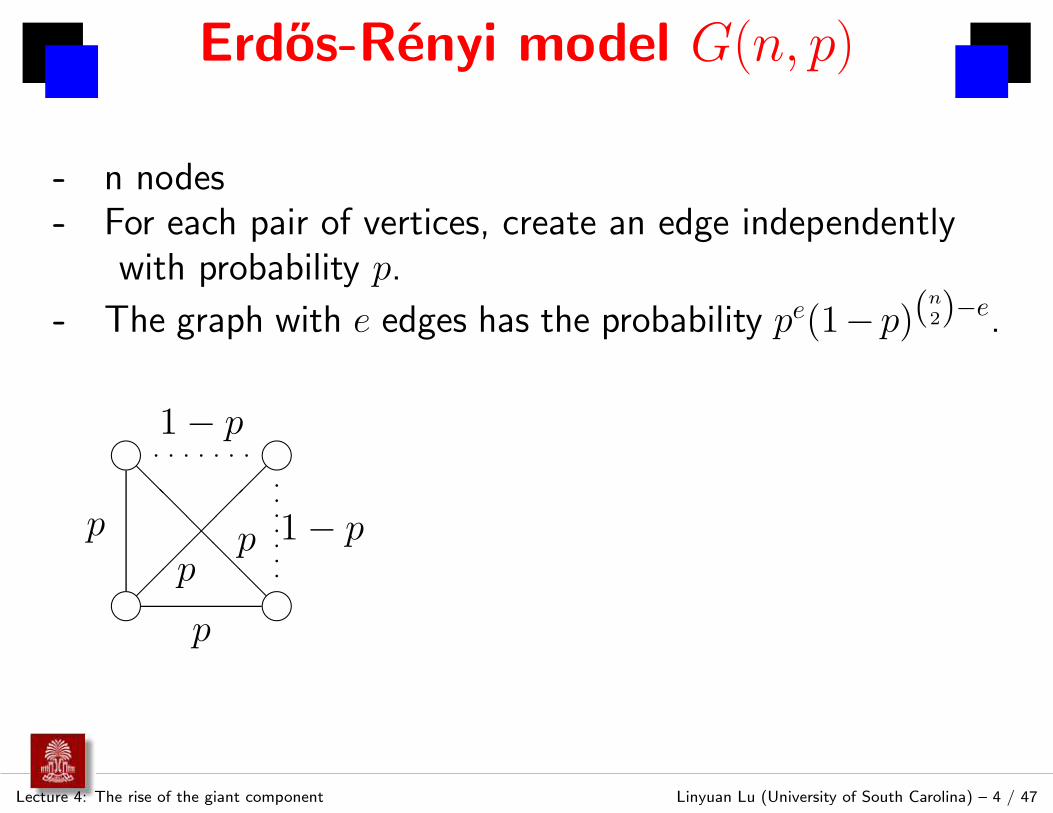
- n nodes

Erdos-Renyi model G(n, p)
Lecture 4: The rise of the giant component Linyuan Lu (University of South Carolina) – 4 / 47
- n nodes- For each pair of vertices, create an edge independently
with probability p.

Erdos-Renyi model G(n, p)
Lecture 4: The rise of the giant component Linyuan Lu (University of South Carolina) – 4 / 47
- n nodes- For each pair of vertices, create an edge independently
with probability p.
- The graph with e edges has the probability pe(1− p)(n2)−e.

Erdos-Renyi model G(n, p)
Lecture 4: The rise of the giant component Linyuan Lu (University of South Carolina) – 4 / 47
- n nodes- For each pair of vertices, create an edge independently
with probability p.
- The graph with e edges has the probability pe(1− p)(n2)−e.
j j
j j
@@
@@
@

Erdos-Renyi model G(n, p)
Lecture 4: The rise of the giant component Linyuan Lu (University of South Carolina) – 4 / 47
- n nodes- For each pair of vertices, create an edge independently
with probability p.
- The graph with e edges has the probability pe(1− p)(n2)−e.
j j
j j
@@
@@
@
p
pp
p
Erdos-Renyi model G(n, p)
Lecture 4: The rise of the giant component Linyuan Lu (University of South Carolina) – 4 / 47
- n nodes- For each pair of vertices, create an edge independently
with probability p.
- The graph with e edges has the probability pe(1− p)(n2)−e.
j j
j j
@@
@@
@
p
pp
p
p p p p p p p
ppppppp
1 − p
1 − p
The probability of thisgraph is
p4(1 − p)2.
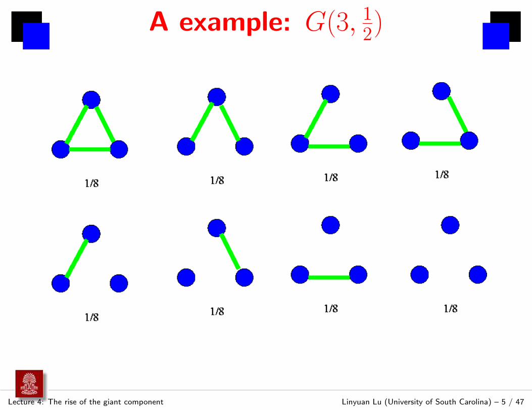
A example: G(3, 12)
Lecture 4: The rise of the giant component Linyuan Lu (University of South Carolina) – 5 / 47

The birth of random graph theory
Lecture 4: The rise of the giant component Linyuan Lu (University of South Carolina) – 6 / 47
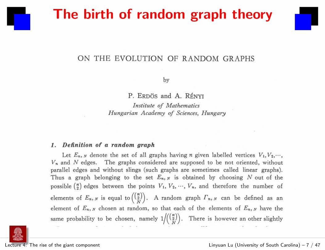
Paul Erdos and A. Renyi, On the evolution of random graphsMagyar Tud. Akad. Mat. Kut. Int. Kozl. 5 (1960) 17-61.
The birth of random graph theory
Lecture 4: The rise of the giant component Linyuan Lu (University of South Carolina) – 7 / 47

Evolution of G(n, p)
Lecture 4: The rise of the giant component Linyuan Lu (University of South Carolina) – 8 / 47
p
0 the empty graph.disjoint union of trees.
cn cycles of any size.1n the double jumps.c′
n one giant component, others are trees.log n
n G(n, p) is connected.
Ω( log nn )
connected and almost regular.Ω(nǫ−1) finite diameter.Θ(1) dense graphs, diameter is 2.1 the complete graph.

Evolution of G(n, p)
Lecture 4: The rise of the giant component Linyuan Lu (University of South Carolina) – 9 / 47
Range I p = o(1/n)The random graph Gn,p is the disjoint union of trees. Infact, trees on k vertices, for k = 3, 4, . . . only appearwhen p is of the order n−k/(k−1).

Evolution of G(n, p)
Lecture 4: The rise of the giant component Linyuan Lu (University of South Carolina) – 9 / 47
Range I p = o(1/n)The random graph Gn,p is the disjoint union of trees. Infact, trees on k vertices, for k = 3, 4, . . . only appearwhen p is of the order n−k/(k−1).
Furthermore, for p = cn−k/(k−1) and c > 0, let τk(G)denote the number of connected components of Gformed by trees on k vertices and λ = (2c)k−1kk−2/k!.Then,
Pr(τk(Gn,p) = j) → λje−λ
j!
for j = 0, 1, . . . as n → ∞.

Evolution of G(n, p)
Lecture 4: The rise of the giant component Linyuan Lu (University of South Carolina) – 10 / 47
Range II p ∼ c/n for 0 < c < 1
In this range of p, Gn,p contains cycles of any givensize with probability tending to a positive limit.
Evolution of G(n, p)
Lecture 4: The rise of the giant component Linyuan Lu (University of South Carolina) – 10 / 47
Range II p ∼ c/n for 0 < c < 1
In this range of p, Gn,p contains cycles of any givensize with probability tending to a positive limit.
All connected components of Gn,p are either trees orunicyclic components. Almost all (i.e., n − o(n))vertices are in components which are trees.
The largest connected component of Gn,p is a treeand has about 1
α(log n − 52 log log n) vertices, where
α = c − 1 − log c.
Evolution of G(n, p)
Lecture 4: The rise of the giant component Linyuan Lu (University of South Carolina) – 11 / 47
Range III p ∼ 1/n + µ/n, the double jump
If µ < 0, the largest component has size(µ − log(1 + µ))−1 log n + O(log log n).
Evolution of G(n, p)
Lecture 4: The rise of the giant component Linyuan Lu (University of South Carolina) – 11 / 47
Range III p ∼ 1/n + µ/n, the double jump
If µ < 0, the largest component has size(µ − log(1 + µ))−1 log n + O(log log n).
If µ = 0, the largest component has size of ordern2/3.

Evolution of G(n, p)
Lecture 4: The rise of the giant component Linyuan Lu (University of South Carolina) – 11 / 47
Range III p ∼ 1/n + µ/n, the double jump
If µ < 0, the largest component has size(µ − log(1 + µ))−1 log n + O(log log n).
If µ = 0, the largest component has size of ordern2/3.
If µ > 0, there is a unique giant component of sizeαn where µ = −α−1 log(1 − α) − 1.
Bollobas showed that a component of size at leastn2/3 in Gn,p is almost always unique if p exceeds1/n + 4(log n)1/2n−4/3.

Evolution of G(n, p)
Lecture 4: The rise of the giant component Linyuan Lu (University of South Carolina) – 12 / 47
Range IV p ∼ c/n for c > 1
Except for one “giant” component, all the othercomponents are relatively small, and most of themare trees.

Evolution of G(n, p)
Lecture 4: The rise of the giant component Linyuan Lu (University of South Carolina) – 12 / 47
Range IV p ∼ c/n for c > 1
Except for one “giant” component, all the othercomponents are relatively small, and most of themare trees.
The total number of vertices in components whichare trees is approximately n − f(c)n + o(n).
The largest connected component of Gn,p hasapproximately f(c)n vertices, where
f(c) = 1 − 1
c
∞∑
k=1
kk−1
k!(ce−c)k.

Evolution of G(n, p)
Lecture 4: The rise of the giant component Linyuan Lu (University of South Carolina) – 13 / 47
Range V p = c log n/n with c ≥ 1
The graph Gn,p almost surely becomes connected.

Evolution of G(n, p)
Lecture 4: The rise of the giant component Linyuan Lu (University of South Carolina) – 13 / 47
Range V p = c log n/n with c ≥ 1
The graph Gn,p almost surely becomes connected.
If
p =log n
kn+
(k − 1) log log n
kn+
y
n+ o(
1
n),
then there are only trees of size at most k except forthe giant component. The distribution of thenumber of trees of k vertices again has a Poissondistribution with mean value e−ky
k·k! .

Evolution of G(n, p)
Lecture 4: The rise of the giant component Linyuan Lu (University of South Carolina) – 14 / 47
Range VI p ∼ ω(n) log n/n where ω(n) → ∞.In this range, Gn,p is not only almost surely connected,but the degrees of almost all vertices are asymptoticallyequal.

Model G(w1, w2, . . . , wn)
Lecture 4: The rise of the giant component Linyuan Lu (University of South Carolina) – 15 / 47
Random graph model with given expected degree sequence
- n nodes with weights w1, w2, . . . , wn.

Model G(w1, w2, . . . , wn)
Lecture 4: The rise of the giant component Linyuan Lu (University of South Carolina) – 15 / 47
Random graph model with given expected degree sequence
- n nodes with weights w1, w2, . . . , wn.
- For each pair (i, j), create an edge independently withprobability pij = wiwjρ, where ρ = 1
∑n
i=1wi
.
- The graph H has probability
∏
ij∈E(H)
pij
∏
ij 6∈E(H)
(1 − pij).
- The expected degree of vertex i is wi.

An example: G(w1, w2, w3, w4)
Lecture 4: The rise of the giant component Linyuan Lu (University of South Carolina) – 16 / 47
@@
@@
@@
@@@

An example: G(w1, w2, w3, w4)
Lecture 4: The rise of the giant component Linyuan Lu (University of South Carolina) – 16 / 47
@@
@@
@@
@@@
w1 w2
w3 w4

An example: G(w1, w2, w3, w4)
Lecture 4: The rise of the giant component Linyuan Lu (University of South Carolina) – 16 / 47
@@
@@
@@
@@@
w1 w2
w3 w4
w1w2ρ
w1w3ρ
w1w4ρ
w2w3ρ

An example: G(w1, w2, w3, w4)
Lecture 4: The rise of the giant component Linyuan Lu (University of South Carolina) – 16 / 47
@@
@@
@@
@@@
w1 w2
w3 w4
w1w2ρ
w1w3ρ
w1w4ρ
w2w3ρ
q q q q q q q1 − w3w4ρ
1 − w2w4ρ
qqqqqqq

An example: G(w1, w2, w3, w4)
Lecture 4: The rise of the giant component Linyuan Lu (University of South Carolina) – 16 / 47
@@
@@
@@
@@@
w1 w2
w3 w4
w1w2ρ
w1w3ρ
w1w4ρ
w2w3ρ
q q q q q q q1 − w3w4ρ
1 − w2w4ρ
qqqqqqq
qqq q qq qqqq
q qqqqqqq q q
1 − w2
1ρ
1 − w2
2ρ
1 − w2
3ρ
1 − w2
4ρ

An example: G(w1, w2, w3, w4)
Lecture 4: The rise of the giant component Linyuan Lu (University of South Carolina) – 16 / 47
@@
@@
@@
@@@
w1 w2
w3 w4
w1w2ρ
w1w3ρ
w1w4ρ
w2w3ρ
q q q q q q q1 − w3w4ρ
1 − w2w4ρ
qqqqqqq
qqq q qq qqqq
q qqqqqqq q q
1 − w2
1ρ
1 − w2
2ρ
1 − w2
3ρ
1 − w2
4ρ
The probability of the graph is
w31w
22w
23w4ρ
4(1 − w2w4ρ) × (1 − w3w4ρ)4
∏
i=1
(1 − w2i ρ).

A example: G(1, 2, 1)
Lecture 4: The rise of the giant component Linyuan Lu (University of South Carolina) – 17 / 47
Loops are omitted here.

Notations
Lecture 4: The rise of the giant component Linyuan Lu (University of South Carolina) – 18 / 47
For G = G(w1, . . . , wn), let
- d = 1n
∑ni=1 wi
- d =∑n
i=1w2
i∑n
i=1wi
.
- The volume of S: Vol(S) =∑
i∈S wi.
Notations
Lecture 4: The rise of the giant component Linyuan Lu (University of South Carolina) – 18 / 47
For G = G(w1, . . . , wn), let
- d = 1n
∑ni=1 wi
- d =∑n
i=1w2
i∑n
i=1wi
.
- The volume of S: Vol(S) =∑
i∈S wi.
We haved ≥ d
“=” holds if and only if w1 = · · · = wn.

Notations
Lecture 4: The rise of the giant component Linyuan Lu (University of South Carolina) – 18 / 47
For G = G(w1, . . . , wn), let
- d = 1n
∑ni=1 wi
- d =∑n
i=1w2
i∑n
i=1wi
.
- The volume of S: Vol(S) =∑
i∈S wi.
We haved ≥ d
“=” holds if and only if w1 = · · · = wn.
A connected component S is called a giant component if
vol(S) = Θ(vol(G)).

Classical result on G(n, p)
Lecture 4: The rise of the giant component Linyuan Lu (University of South Carolina) – 19 / 47
If np < 1, almost surely there is no giant component.
If np > 1, almost surely there is a unique giantcomponent.
d = d = np.

Four questions
Lecture 4: The rise of the giant component Linyuan Lu (University of South Carolina) – 20 / 47
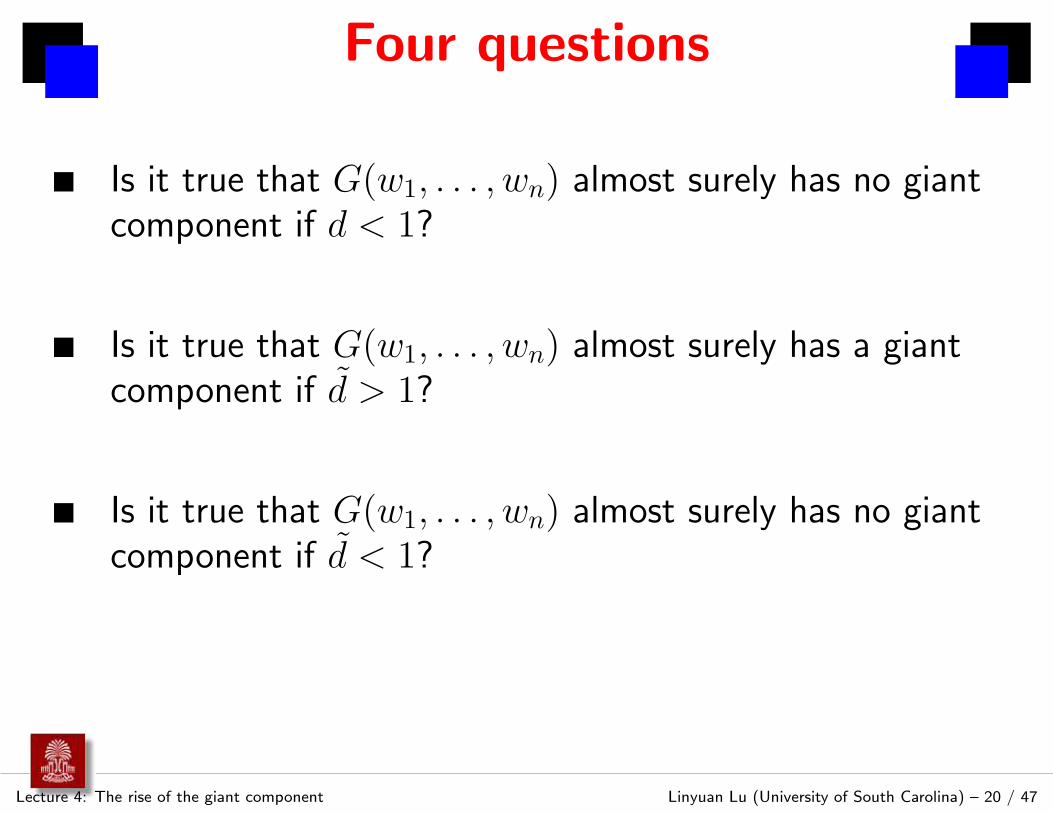
Is it true that G(w1, . . . , wn) almost surely has no giantcomponent if d < 1?

Four questions
Lecture 4: The rise of the giant component Linyuan Lu (University of South Carolina) – 20 / 47
Is it true that G(w1, . . . , wn) almost surely has no giantcomponent if d < 1?
Is it true that G(w1, . . . , wn) almost surely has a giantcomponent if d > 1?
Four questions
Lecture 4: The rise of the giant component Linyuan Lu (University of South Carolina) – 20 / 47
Is it true that G(w1, . . . , wn) almost surely has no giantcomponent if d < 1?
Is it true that G(w1, . . . , wn) almost surely has a giantcomponent if d > 1?
Is it true that G(w1, . . . , wn) almost surely has no giantcomponent if d < 1?
Is it true that G(w1, . . . , wn) almost surely has a giantcomponent if d > 1?

Case d < 1
Lecture 4: The rise of the giant component Linyuan Lu (University of South Carolina) – 21 / 47
Is it true that G(w1, . . . , wn) almost surely has no giantcomponent if d < 1?

Case d < 1
Lecture 4: The rise of the giant component Linyuan Lu (University of South Carolina) – 21 / 47
Is it true that G(w1, . . . , wn) almost surely has no giantcomponent if d < 1?
No.

Case d < 1
Lecture 4: The rise of the giant component Linyuan Lu (University of South Carolina) – 21 / 47
Is it true that G(w1, . . . , wn) almost surely has no giantcomponent if d < 1?
No. A counter-example: G(n2 , 0) + G(n
2 ,3n).
Since G(n2 ,
3n) has
n′p′ =n
2
3
n=
3
2> 1.
It has a giant component. But as the whole graph, theaverage degree is d = 3
4 < 1.

Case d > 1
Lecture 4: The rise of the giant component Linyuan Lu (University of South Carolina) – 22 / 47
Is it true that G(w1, . . . , wn) almost surely has a giantcomponent if d > 1?

Case d > 1
Lecture 4: The rise of the giant component Linyuan Lu (University of South Carolina) – 22 / 47
Is it true that G(w1, . . . , wn) almost surely has a giantcomponent if d > 1?
No.
Case d > 1
Lecture 4: The rise of the giant component Linyuan Lu (University of South Carolina) – 22 / 47
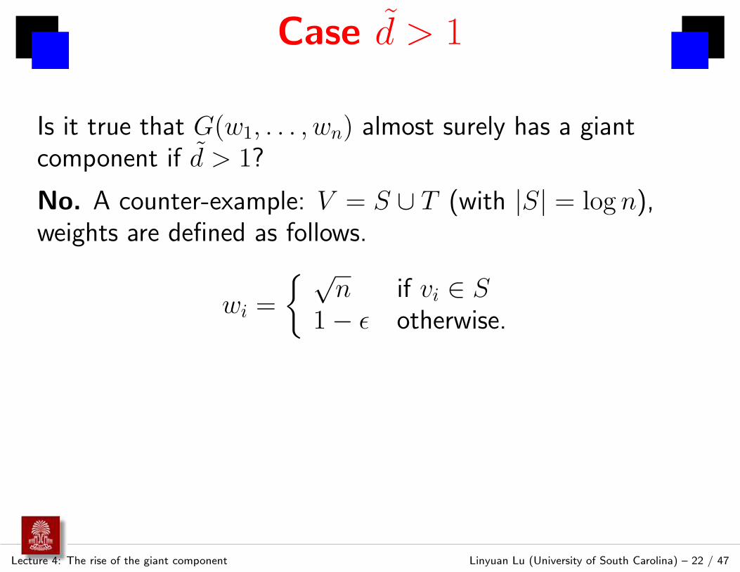
Is it true that G(w1, . . . , wn) almost surely has a giantcomponent if d > 1?
No. A counter-example: V = S ∪ T (with |S| = log n),weights are defined as follows.
wi =
√n if vi ∈ S
1 − ǫ otherwise.

Case d > 1
Lecture 4: The rise of the giant component Linyuan Lu (University of South Carolina) – 22 / 47
Is it true that G(w1, . . . , wn) almost surely has a giantcomponent if d > 1?
No. A counter-example: V = S ∪ T (with |S| = log n),weights are defined as follows.
wi =
√n if vi ∈ S
1 − ǫ otherwise.Every component in G|T has size at most O(log n). AddingS can join at most O(
√n log2 n) vertices in T . The volume
of maximum component is at most O(√
n log2 n).
d =n log n + (1 − ǫ)(n − log n)
√n log n +
√
(1 − ǫ)(n − log n)> log n.
Case d < 1
Lecture 4: The rise of the giant component Linyuan Lu (University of South Carolina) – 23 / 47
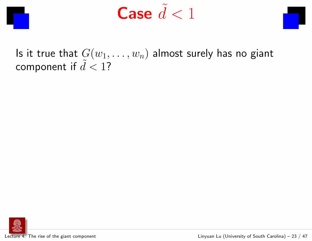
Is it true that G(w1, . . . , wn) almost surely has no giantcomponent if d < 1?

Case d < 1
Lecture 4: The rise of the giant component Linyuan Lu (University of South Carolina) – 23 / 47
Is it true that G(w1, . . . , wn) almost surely has no giantcomponent if d < 1?
Yes. Chung and Lu (2001) Suppose that d < 1 − δ. For
any α > 0, with probability at least 1 − dd2
α2(1−d), a random
graph G in G(w1, . . . , wn) has all connected componentswith volume at most α
√n.

Proof
Lecture 4: The rise of the giant component Linyuan Lu (University of South Carolina) – 24 / 47
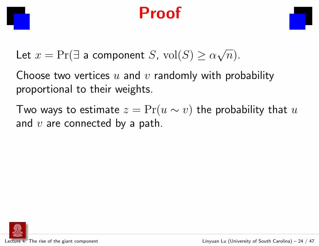
Let x = Pr(∃ a component S, vol(S) ≥ α√
n).

Proof
Lecture 4: The rise of the giant component Linyuan Lu (University of South Carolina) – 24 / 47
Let x = Pr(∃ a component S, vol(S) ≥ α√
n).
Choose two vertices u and v randomly with probabilityproportional to their weights.
Proof
Lecture 4: The rise of the giant component Linyuan Lu (University of South Carolina) – 24 / 47
Let x = Pr(∃ a component S, vol(S) ≥ α√
n).
Choose two vertices u and v randomly with probabilityproportional to their weights.
Two ways to estimate z = Pr(u ∼ v) the probability that uand v are connected by a path.
One the one hand,
z ≥ Pr(u ∼ v, ∃ a component S vol(S) ≥ α√
n)
= Pr(u ∼ v | ∃ a component S vol(S) ≥ α√
n)x
≥ Pr(u, v ∈ S | ∃ a component S vol(S) ≥ α√
n)x
≥ α2nρ2x.

Proof
Lecture 4: The rise of the giant component Linyuan Lu (University of South Carolina) – 25 / 47
On the other hand, the probability Pk(u, v) of u and v beingconnected by a path of length k + 1 is at most
Pk(u, v) ≤∑
i1,i2,...,ik
(wuwi1ρ) (wi1wi2ρ) · · · (wikwvρ)
= wuwvρdk.

Proof
Lecture 4: The rise of the giant component Linyuan Lu (University of South Carolina) – 25 / 47
On the other hand, the probability Pk(u, v) of u and v beingconnected by a path of length k + 1 is at most
Pk(u, v) ≤∑
i1,i2,...,ik
(wuwi1ρ) (wi1wi2ρ) · · · (wikwvρ)
= wuwvρdk.
The probability that u and v are connected is at most
n∑
k=0
Pk(u, v) ≤∑
k≥0
wuwvρdk =1
1 − dwuwvρ.

Proof
Lecture 4: The rise of the giant component Linyuan Lu (University of South Carolina) – 26 / 47
z ≤∑
u,v
wuρ wvρ1
1 − wwuwvρ =
d2
1 − dρ.
Combining this with z ≥ xα2nρ2
we have
α2xnρ2 ≤ d2
1 − dρ
which implies that
x ≤ dd2
α2(1 − d).
The proof is finished.

Case d > 1
Lecture 4: The rise of the giant component Linyuan Lu (University of South Carolina) – 27 / 47
Gap theorem:
Almost surely G has a unique giant component (GCC).
vol(GCC) ≥
(1 − 2√de
+ o(1))Vol(G) if d ≥ 4e .
(1 − 1+log dd + o(1))Vol(G) if d < 2.
The second largest component almost surely has size atmost (1 + o(1))µ(d) log n, where
µ(d) =
11+log d−log 4 if d > 4/e;
1d−1−log d if 1 < d < 2.
Matrix-tree theorem
Lecture 4: The rise of the giant component Linyuan Lu (University of South Carolina) – 28 / 47
Kirchhofff (1847) The number of spanning trees in agraph G is equal to any cofactor of L = D − A, whereD = diag(d1, . . . , dn) is the diagonal degree matrix and A isthe adjacency matrix.
The matrix-tree theorem holds for weighted graphs.
∑
T
∏
f∈E(T )
we = | det M |.
Here M is obtained by deleting one row and one columnfrom D − A.

A set S as component
Lecture 4: The rise of the giant component Linyuan Lu (University of South Carolina) – 29 / 47
Let S = vi1, vi2 . . . , vik with weights wi1, wi2, . . . , wik . Theprobability that there is no edge leaving S is
∏
vi∈S,vj 6∈S (1 − wiwjρ)
≈ e−ρ
∑
vi∈S,vj 6∈S wiwj
= e−ρvol(S)(vol(G)−vol(S)).
The probability G |S is connected is at most
∑
T
∏
(vijvil
)∈E(T )
wijwilρ = wi1wi2 · · ·wikvol(S)k−2ρk−1.
Computation is done by matrix-tree theorem.
Detail computation
Lecture 4: The rise of the giant component Linyuan Lu (University of South Carolina) – 30 / 47
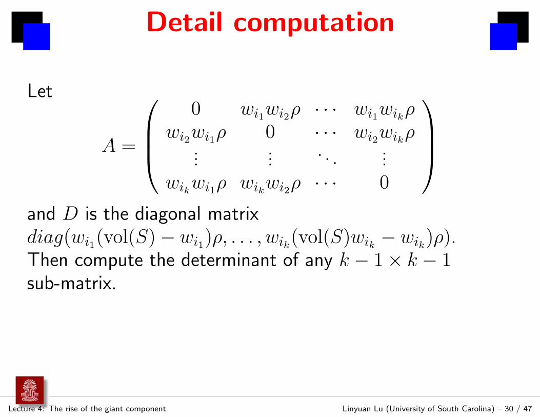
Let
A =
0 wi1wi2ρ · · · wi1wikρwi2wi1ρ 0 · · · wi2wikρ
...... . . . ...
wikwi1ρ wikwi2ρ · · · 0
and D is the diagonal matrixdiag(wi1(vol(S) − wi1)ρ, . . . , wik(vol(S)wik − wik)ρ).Then compute the determinant of any k − 1 × k − 1sub-matrix.

A set S as component
Lecture 4: The rise of the giant component Linyuan Lu (University of South Carolina) – 31 / 47
The probability that S is a component is at most
∑
S
wi1wi2 · · ·wikvol(S)k−2ρk−1e−vol(S)(1−vol(S)/vol(G)).
The probability that there exists a connected component onsize k with volume less than ǫvol(G) is at most
f(k, ǫ) =∑
|S|=k
wi1wi2 · · ·wikvol(S)k−2ρk−1e−vol(S)(1−ǫ).

Case d > 4e(1−ǫ)2
Lecture 4: The rise of the giant component Linyuan Lu (University of South Carolina) – 32 / 47
f(k, ǫ) =∑
S
wi1wi2 · · ·wikvol(S)k−2ρk−1e−vol(S)(1−ǫ)
≤∑
S
ρk−1
kkvol(S)2k−2e−vol(S)(1−ǫ)
≤∑
S
ρk−1
kk(2k − 2
1 − ǫ)2k−2e−(2k−2)
≤ nk
k!
ρk−1
kk(2k − 2
1 − ǫ)2k−2e−(2k−2)
≤ 1
4ρ(k − 1)2(
4
de(1 − ǫ)2)k

Case 11−ǫ < d < 2
1−ǫ
Lecture 4: The rise of the giant component Linyuan Lu (University of South Carolina) – 33 / 47
First, we split f(k, ǫ) into two parts as follows:
f(k, ǫ) = f1(k, ǫ) + f2(k, ǫ)
where
f1(k, ǫ) =∑
vol(S)<dk
wi1wi2 · · ·wikvol(S)k−2ρk−1e−vol(S)(1−ǫ)
f2(k, ǫ) =∑
vol(S)≥dk
wi1wi2 · · ·wikvol(S)k−2ρk−1e−vol(S)(1−ǫ)

Bounding f1(k, ǫ)
Lecture 4: The rise of the giant component Linyuan Lu (University of South Carolina) – 34 / 47
f1(k, ǫ) =∑
vol(S)<dk
wi1 · · ·wikvol(S)k−2ρk−1e−vol(S)(1−ǫ)
≤∑
vol(S)<dk
ρk−1
kkvol(S)2k−2e−vol(S)(1−ǫ)
≤∑
vol(S)<dk
ρk−1
kk(dk)2k−2e−dk(1−ǫ)
≤(
n
k
)
ρk−1
kk(dk)2k−2e−dk(1−ǫ)
≤ n
dk2(
d
ed(1−ǫ)−1)k

Bounding f2(k, ǫ)
Lecture 4: The rise of the giant component Linyuan Lu (University of South Carolina) – 35 / 47
f2(k, ǫ) =∑
vol(S)≥dk
wi1wi2 · · ·wikvol(S)k−2ρk−1e−vol(S)(1−ǫ)
≤∑
vol(S)≥dk
wi1 · · ·wikρk−1(dk)k−2e−dk(1−ǫ)
≤∑
S
wi1wi2 · · ·wikρk−1(dk)k−2e−dk(1−ǫ)
<vol(G)k
k!ρk−1(dk)k−2e−dk(1−ǫ)
≤ n
dk2(
d
e(d(1−ǫ)−1))k

Put together
Lecture 4: The rise of the giant component Linyuan Lu (University of South Carolina) – 36 / 47
If d > 4e(1−ǫ)2 , then
f(k, ǫ) ≤ 1
4ρ(k − 1)2(
4
de(1 − ǫ)2)k.
If 11−ǫ < d < 2
1−ǫ , then
f(k, ǫ) ≤ 2n
dk2(
d
e(d(1−ǫ)−1))k.
Choose k = µ(d) log n, then f(k, ǫ) = o(1). The gaptheorem is proved.

Volume of Giant Component
Lecture 4: The rise of the giant component Linyuan Lu (University of South Carolina) – 37 / 47
Chung and Lu (2004)If the average degree is strictly greater than 1, then almostsurely the giant component in a graph G in G(w) has
volume (λ0 + O(√
n log3.5 nVol(G) )
)
Vol(G), where λ0 is the unique
positive root of the following equation:
n∑
i=1
wie−wiλ = (1 − λ)
n∑
i=1
wi.
Sketch proof
Lecture 4: The rise of the giant component Linyuan Lu (University of South Carolina) – 38 / 47
With probability at least 1 − 2n−k, a vertex with weightgreater than max8k, 2(k + 1 + o(1))µ(d) log n is inthe GCC.

Sketch proof
Lecture 4: The rise of the giant component Linyuan Lu (University of South Carolina) – 38 / 47
With probability at least 1 − 2n−k, a vertex with weightgreater than max8k, 2(k + 1 + o(1))µ(d) log n is inthe GCC.
For any k > 2, with probability at least 1 − 6n−k+2, wehave |Vol(GCC) − E(Vol(GCC))| ≤2C1(k + 1)2
√k − 2
√n log2.5 n, where
C1 = 10µ(d) + 2µ(d)2.
Vol(G) − E(vol(GCC)) =∑
wv<Ck log n wve−wvE(Vol(GCC))ρ + O(k3
√n log3.5 n).

Lagrange inversion formula
Lecture 4: The rise of the giant component Linyuan Lu (University of South Carolina) – 39 / 47
Suppose that z is a function of x and y in terms of another
analytic function φ as follows:
z = x + yφ(z).
Then z can be written as a power series in y as follows:
z = x +∞
∑
k=1
yk
k!D(k−1)φk(x)
where D(t) denotes the t-th derivative.

Apply it to G(n, p)
Lecture 4: The rise of the giant component Linyuan Lu (University of South Carolina) – 40 / 47
For the G(n, p), the equation is simply e−dλ = (1 − λ). Letλ = 1 − z
d . We have z = de−dez.

Apply it to G(n, p)
Lecture 4: The rise of the giant component Linyuan Lu (University of South Carolina) – 40 / 47
For the G(n, p), the equation is simply e−dλ = (1 − λ). Letλ = 1 − z
d . We have z = de−dez. We apply Lagrange
inversion formula with x = 0, y = de−d, and φ(z) = ez.Then we have
z =∞
∑
k=1
yk
k!D(k−1)ekx |x=0
=∞
∑
k=1
kk−1
k!(de−d)k
This is exactly Erdos and Renyi’s result on G(n, p).

G(n, p) verse G(w1, . . . , wn)
Lecture 4: The rise of the giant component Linyuan Lu (University of South Carolina) – 41 / 47
Question: Does the random graph with equal expecteddegrees generates the smallest giant component among allpossible degree distribution with the same volume?

G(n, p) verse G(w1, . . . , wn)
Lecture 4: The rise of the giant component Linyuan Lu (University of South Carolina) – 41 / 47
Question: Does the random graph with equal expecteddegrees generates the smallest giant component among allpossible degree distribution with the same volume?Chung Lu (2004)
Yes, for 1 < d ≤ ee−1 .
No, for sufficiently large d.

G(n, p) verse G(w1, . . . , wn)
Lecture 4: The rise of the giant component Linyuan Lu (University of South Carolina) – 41 / 47
Question: Does the random graph with equal expecteddegrees generates the smallest giant component among allpossible degree distribution with the same volume?Chung Lu (2004)
Yes, for 1 < d ≤ ee−1 .
No, for sufficiently large d. When d ≥ 4
e , almost surely the giant component ofG(w1, . . . , wn) has volume at least
(
1
2
(
1 +
√
1 − 4
de
)
+ o(1)
)
Vol(G).
This is asymptotically best possible.

Sizes and edges in GCC
Lecture 4: The rise of the giant component Linyuan Lu (University of South Carolina) – 42 / 47
Chung, Lu (2004) If the expected average degree is strictly
greater than 1, then almost surely the giant component in a
random graph of given expected degrees wi, i = 1, . . . , n,
has n − ∑ni=1 e−wiλ0 + O(
√n log3.5 n) vertices and
(λ0 − 12λ
20)Vol(G) + O(
√
Vol(G) log3.5 n) edges.

In the collaboration graph
Lecture 4: The rise of the giant component Linyuan Lu (University of South Carolina) – 43 / 47
λ0(2 − λ0) ≈Vol(GCC)
Vol(G)≈ 248000
284000.
We have λ0 ≈ 0.644.Let nk denote the number of vertices of degree k. We have
nk ≈ E(nk) ≈∑
i≥0
wki
k!e−wi.
n0 n1 n2 n3 n4 n5 n6 n7 n8 n9
166381 145872 34227 16426 9913 6670 4643 3529 2611 2032

Compute |GCC|
Lecture 4: The rise of the giant component Linyuan Lu (University of South Carolina) – 44 / 47
|GCC| ≈ n −n
∑
i=1
e−λ0wi
= n −n
∑
i=1
e(1−λ0)wie−wi
=∑
k≥0
nk −n
∑
i=1
∞∑
k=0
(1 − λ0)k
k!wk
i e−wi
≈∑
k≥0
nk(1 − (1 − λ0)k)
=∑
k≥1
nk(1 − (1 − λ0)k).
Conclusion
Lecture 4: The rise of the giant component Linyuan Lu (University of South Carolina) – 45 / 47
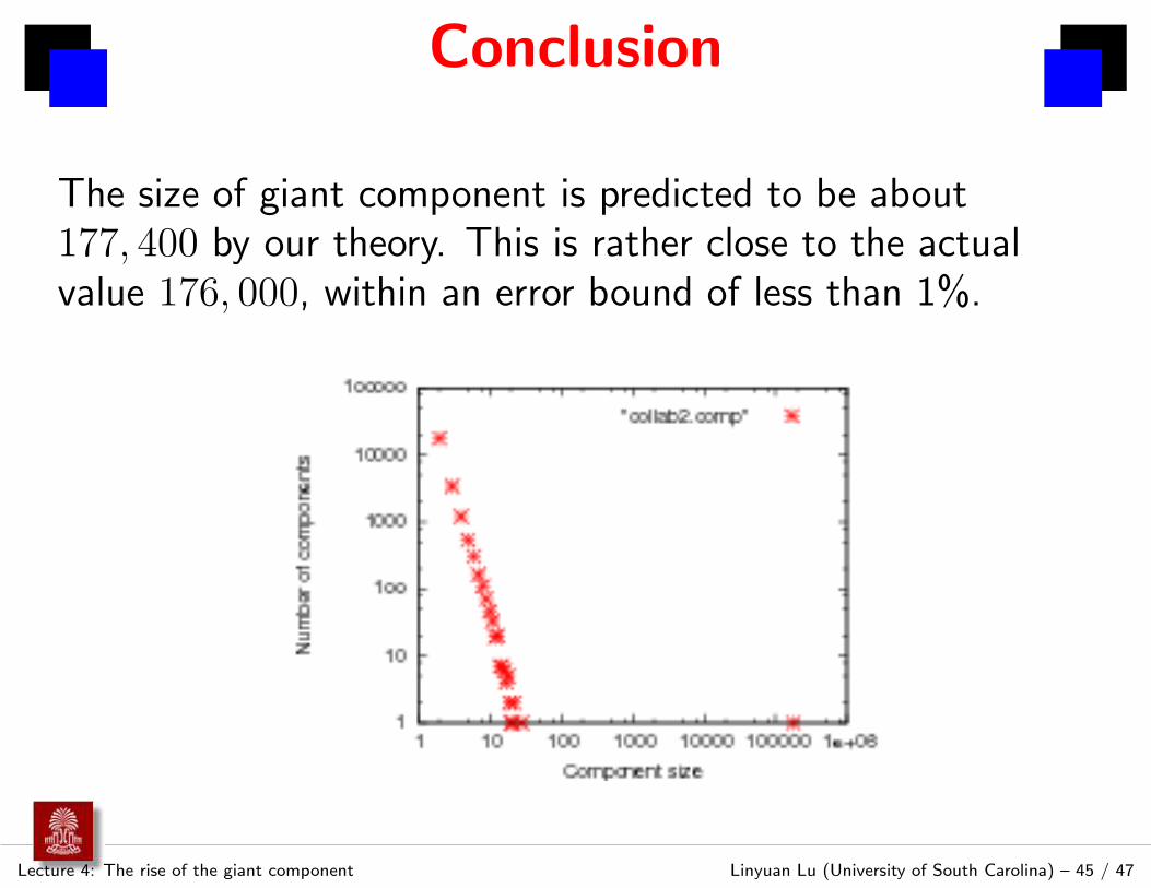
The size of giant component is predicted to be about177, 400 by our theory. This is rather close to the actualvalue 176, 000, within an error bound of less than 1%.
References
Lecture 4: The rise of the giant component Linyuan Lu (University of South Carolina) – 46 / 47
Fan Chung and Linyuan Lu. Connected components in arandom graph with given degree sequences, Annals of
Combinatorics, 6 (2002), 125–145.
Fan Chung and Linyuan Lu, The volume of the giantcomponent for a random graph with given expecteddegrees , SIAM J. Discrete Math., 20 (2006), No. 2,395–411.
Overview of talks
Lecture 4: The rise of the giant component Linyuan Lu (University of South Carolina) – 47 / 47
Lecture 1: Overview and outlines
Lecture 2: Generative models - preferential attachmentschemes
Lecture 3: Duplication models for biological networks
Lecture 4: The rise of the giant component
Lecture 5: The small world phenomenon: averagedistance and diameter
Lecture 6: Spectrum of random graphs with givendegrees


