
Technological University Lashio Journal of Research & Innovation Vol. 1, Issue: 1
TULSOJRI September, 2020 156
Comparative Study On Optimum Shear Wall Contribution in Design at Eighteen Storeyed
Reinforce Concrete Residential Building
Kyaw Naing(1), Sunday Aung(2)
(1)Technological University (Lashio), Myanmar
(2)Technological University (Lashio), Myanmar
Email: [email protected], [email protected]
ABSTRACT: Multistorey buildings are the symbols of a modernized living standard because of the population growth. South East Asia including Myanmar is situated in secondary seismic belt. Therefore, it is necessary to pay special attention of the effect of earthquake in designing the high-rise building.
Shear walls are very common in high-rise reinforced concrete building. In this study, comparative study of shear wall contribution for eighteen-storeyed reinforced concrete building are present. It belongs to seismic zone 2A. This is why, seismic forces are essentially considered in the design of this building and shear walls are also considered to resist seismic forces.
Structural analysis is done by using ETABS software. Load consideration is based on UBC-1997. All necessary load combinations are considered in shear walls analysis and frame analysis. In addition to this study gravity load and lateral load are considered. Design of structural elements are calculated by using the provision of American Concrete Institute (ACI 318-99) code.
The selected building with seven different locations of shear walls are analyzed and checked for stability. Then eccentricity required steel area and allowable values for torsional irregularity, overturning and sliding are compared to point out the best location of shear wall. Design results are checked for safety,
economy and serviceability by checking in P- effect, storey drift, structural irregularity, sliding and overturning.
KEYWORDS: Gravity load and lateral load, ETABS Software, Eighteen-Storey Building, Planar Shear Wall, Regular Shape, ACI 318-99,UBC-97.
1. INTRODUCTION
According to social and economical demands, presently, Yangon, needs various types of tall buildings. These buildings are the solutions to the problem of living population growth. Because they form distinctive landmarks, tall buildings are frequently developed in central business zone as prestige symbols for corporate organization. The feasibility and desirability of high-rise structure have always depended on the available materials, the level of construction technology, and the state of development of the services necessary for the use of the building. It is important to ensure adequate stiffness to resist lateral forces induced by wind or seismic or blast effects. These forces can develop high
stresses, and produce, way moment or vibration. Concrete walls, which have high in-plane stiffness placed at convenient locations, are often economically used to provide the necessary resistance to horizontal forces. This type of wall is called a shear wall.
To obtain the required stiffness and strength to withstand lateral load in high- rise building, shear walls are normally included some frames of the building. They are continuous down to the base to which they are rigidly attached to form vertical cantilever. The positions of shear walls within a building are dictated by functional requirements. They may or may not suit structural planning. Building sites, architectural interests may lead, on the other hand, to positions of walls that one undesirable from a structural point of view. Hence, structural designers will often be in the position desirable locations for shear wall in order to optimize lateral force resistance. Shear wall are efficient, both in terms of construction cost and effectiveness in minimizing earthquake damage in structural and non- structural
2. THEORETICAL BACKGROUND
2.1 Scope of the Study
The scope of the study is defined as follows: 1. The proposed building is eighteen storied R.C.C
building in seismic zone 2A. 2. Only planar shear walls are considered 3. Structural analysis and design are to be done by
ETABS. 4. Load consideration is based on UBC Code
( 1997 ). 5. Structural elements are designed according to
ACI- 318-99. 2.2 Material Properties of the Structure
Material properties used in this structure are; weight per unit volume (R.C); w = 150 lb/ft3, concrete strength fc' = 3ksi; reinforced yield strength= 50 ksi, Poisson's ratio= 0.175.
2.3 Loading
(1) Dead load Unit weight of concrete = 150 lb/ft3 4½" thick wall weight = 55lb/ft2 9" thick wall weight = 100 lb/ft2 Ceiling weight = 25 lb/ft2 Floor finishing = 10 lb/ft2 (2) Live load Live load on residential = 40 lb/ft2
Technological University Lashio Journal of Research & Innovation Vol. 1, Issue: 1
TULSOJRI September, 2020 157
Live load on roof = 20 lb/ft2 (3) Wind load Exposure type = Type C Basic wind velocity = 80 mph Important factor = 1 Windward coefficient = 0.8 Leeward coefficient = 0.5 (4) Earthquake load
Seismic zone = zone 2A (Yangon)
Zone factor (Z) = 0.15 Soil type = SD Importance factor (I) = 1.0 Response modification factor (R) = 6.5 Seismic coefficient (Ca) = 0.22 Na Seismic coefficient (Cv) = 0.32 Nv Near source factor (Na) = 1.0 Near source factor (Nv) = 1.0 seismic source type = A
3. ANALYSIS AND DESIGN
The selected structure is eighteen-storeyed reinforced concrete building. The building is located in Seismic Zone 2A. It is analyzed to meet the requirements of the Uniform Building Code (UBC), 1997.The building is symmetric about both principal plan axes. In this building, dual system is used for resistance to gravity and lateral loads.
3.1 Modeling of Non- Shear Wall Structure
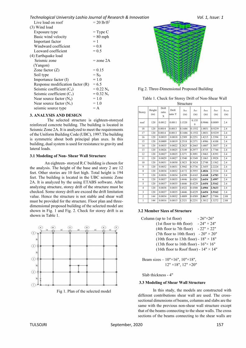
An eighteen- storyed R.C building is chosen for the analysis. The height of the base and story 2 are 12 feet. Other stories are 10 feet high. Total height is 194 feet. The building is located in the UBC seismic Zone 2A. It is analyzed by the using ETABS software. After analyzing structure, storey drift of the structure must be checked. Some storey drift are exceed the drift limitation value. Hence the structure is not stable and shear wall must be provided for the structure. Floor plan and three- dimensional proposed building of the selected model are shown in Fig. 1 and Fig. 2. Check for storey drift is as shown in Table 1.
Fig 1. Plan of the selected model
Fig 2. Three-Dimensional Proposed Building
Table 1. Check for Storey Drift of Non-Shear Wall
Structure
Storey Height
(in)
Drift
ratio
X
Drift
ratio Y
SX
(in)
SY
(in)
MX (in)
MY (in)
Limit (in)
roof 120 0.0012 0.0011 0.1520 0.135
9 0.9046 0.8089 2.4
18 120 0.0014 0.0013 0.1686 0.1552 1.0031 0.9239 2.4
17 120 0.0014 0.0013 0.1686 0.1552 1.0031 0.9239 2.4
16 120 0.0019 0.0018 0.2389 0.2251 1.4215 1.3394 2.4
15 120 0.0009 0.0019 0.2518 0.2371 1.4986 1.4108 2.4
14 120 0.0035 0.0022 0.2825 0.2665 1.6807 1.5857 2.4
13 120 0.0026 0.0025 0.3149 0.2977 1.8735 1.7744 2.4
12 120 0.0027 0.0025 0.3271 0.3091 1.9463 1.8393 2.4
11 120 0.0029 0.0027 0.3540 0.3349 2.1063 1.9928 2.4
10 120 0.0031 0.0030 0.3823 0.3624 2.2748 2.1562 2.4
9 120 0.0032 0.0031 0.3942 0.3736 2.3455 2.2224 2.4
8 120 0.0034 0.0032 0.4172 0.3955 2.4826 2.3534 2.4
7 120 0.0036 0.0034 0.4398 0.4165 2.6168 2.4783 2.4
6 120 0.0037 0.0035 0.4446 0.4201 2.6454 2.4997 2.4
5 120 0.0037 0.0035 0.4446 0.4229 2.6454 2.5162 2.4
4 120 0.0038 0.0035 0.4522 0.4308 2.6904 2.5633 2.4
3 120 0.0037 0.0035 0.4446 0.4229 2.6454 2.5162 2.4
2 144 0.0034 0.0032 0.4809 0.4589 2.8617 2.7306 2.88
1 144 0.0016 0.0015 0.2321 0.2231 1.3812 1.3272 2.88
3.2 Member Sizes of Structure
Column (up to 1st floor) - 26"×26"
(1st floor to 4th floor) - 24" × 24''
(4th floor to 7th floor) - 22" × 22"
(7th floor to 10th floor) - 20" × 20"
(10th floor to 13th floor) - 18" × 18"
(13th floor to 16th floor) - 16"× 16"
(16th floor to Roof floor) - 14" × 14"
Beam sizes – 10"×16", 10"×18",
12" ×18", 12" ×20"
Slab thickness - 4"
3.3 Modeling of Shear Wall Structure
In this study, the models are constructed with
different contributions shear wall are used. The cross-
sectional dimensions of beams, columns and slabs are the
same with the previous non-shear wall structure except
that of the beams connecting to the shear walls. The cross
sections of the beams connecting to the shear walls are

Technological University Lashio Journal of Research & Innovation Vol. 1, Issue: 1
TULSOJRI September, 2020 158
taken as 12"×24". The material properties, loading and
other data for wind and seismic forces are the same as the
non-shear wall structure. The thickness of shear walls
are:
Shear walls (up to 1st floor) - 22"
(1st floor to 4th floor) - 20"
(4th floor to 7th floor) - 18"
(7th floor to 10th floor) - 16"
(10th floor to 13th floor) - 14"
(13th floor to 16th floor) - 12"
(16th floor to Roof floor) - 10"
3.4 Locations of Shear Wall Contribution
Fig 3. Model-1
Fig 4. Model-2
Fig 5. Model-3
Fig 6. Model-4
Fig 7. Model-5
Fig 8. Model-6
Fig 9. Model-7
Fig 10. Model-8
Fig 11. Model-9

Technological University Lashio Journal of Research & Innovation Vol. 1, Issue: 1
TULSOJRI September, 2020 159
Fig 12. Model-10
Fig 13. Model-11
Fig 14. Model-12
Fig 15. Model-13
Fig 16. Model-14
4. CHECK FOR STABILITY OF STRUCTURE
A. Overturning Moment The safety factor for both X and Y direction
have greater than 1.5. Therefore, the structure is capable of resisting overturning effect.
B. Sliding The ratio of the Resistance to friction to sliding
force is called factor of safety for sliding. For these proposed building, the factor of safety for sliding is greater than that of 1.5. Therefore, there is no sliding occur in the structure. Sliding and overturning moment is occurred in model-(7) & (10) because the factor of safety is less than 1.5.
C. Storey Drift The storey drifts are checked in order to
determine whether the structure is stable or not by using UBC- 97 formula.
= 0.7 RDs < Limit where,
= Maximum storey drift
S = Storey drift obtained from the analysis
R = Response modification factor = 8.5
Limit = Storey drift limitation = 2.0% of story height for T>0.7 sec
D. Torsional Irregularity The maximum drift at one end of the structure
transverse to its axis is not more than 1.2 times the average storey drifts of both ends. The selected building with fourteen different
locations of planar shear walls are analyzed and checked
for stability. From those checking, model (1), (2), (3),
(4), (5), (6), (8), (9), (11), (12), (13) and (14) are selected
as the desirable models for storey drift of shear walls.
The comparative studies on results for these models are
shown in Table 2.
Table 2(A). Check for Storey Drift of Model (1), (2) & (3)
Model (1) Model (2) Model (3)
Storey MX (in)
MY (in)
MX (in)
MY (in)
MX (in)
MY (in)
roof 1.460 1.1788 1.3823 1.1531 1.3980 1.2023
18 1.522 1.2216 1.4301 1.1980 1.4929 1.2516
17 1.599 1.270 1.4651 1.2337 1.586 1.2980
16 1.662 1.3080 1.4715 1.2423 1.6350 1.3187
15 1.677 1.3159 1.4851 1.2587 1.6957 1.3458

Technological University Lashio Journal of Research & Innovation Vol. 1, Issue: 1
TULSOJRI September, 2020 160
14 1.711 1.3337 1.4922 1.2694 1.7421 1.3637
13 1.738 1.3473 1.382 1.1531 1.7464 1.356
12 1.732 1.3394 1.4786 1.2623 1.7671 1.356
11 1.747 1.3444 1.4751 1.2644 1.78 1.3508
10 1.756 1.3451 1.4644 1.2609 1.7635 1.3272
9 1.735 1.3273 1.4358 1.2409 1.7642 1.310
8 1.722 1.3130 1.4101 1.2237 1.7564 1.2873
7 1.690 1.2823 1.3673 1.192 1.7228 1.2466
6 1.615 1.2216 1.2980 1.1359 1.6943 1.2066
5 1.523 1.1445 1.2145 1.066 1.6443 1.1502
4 1.380 1.0310 1.0974 0.9674 1.556 1.0695
3 1.173 0.872 0.9396 0.8325 1.4494 0.9767
2 1.059 0.7788 0.8747 0.7788 1.2973 0.8560
1 0.463 0.3392 0.4489 0.4018 0.0570 0.4635
Table 2(B). Check for Storey Drift of Model (4), (5) &
(6)
Model (4) Model (5) Model (6)
Storey MX
(in)
MY
(in)
MX
(in)
MY
(in)
MX
(in)
MY
(in)
roof 1.3573 1.4666 1.30519 1.41729 1.54938 1.14097
18 1.3823 1.4894 1.35803 1.46727 1.59936 1.16739
17 1.4144 1.5180 1.38302 1.49012 1.66005 1.19809
16 1.4366 1.5365 1.41515 1.51868 1.70646 1.21879
15 1.4323 1.5272 1.43728 1.53653 1.71074 1.21737
14 1.4359 1.5265 1.43228 1.52796 1.73145 1.22308
13 1.4316 1.5173 1.43585 1.52653 1.74501 1.22308
12 1.4080 1.4894 1.43157 1.51725 1.73002 1.20594
11 1.3930 1.4687 1.36945 1.44014 1.73145 1.19666
10 1.3695 1.4394 1.32804 1.39230 1.72573 1.18024
9 1.3280 1.3923 1.28734 1.34589 1.6936 1.14668
8 1.2881 1.3452 1.22951 1.28092 1.66719 1.11526
7 1.2302 1.2802 1.14954 1.19095 1.62006 1.06743
6 1.1495 1.1902 1.05672 1.08671 1.53438 0.99674
5 1.0581 1.0853 0.93320 0.95248 1.43014 0.91463
4 0.9339 0.9518 0.77398 0.78611 1.28234 0.8061
3 0.7747 0.7854 0.67516 0.68287 1.08099 0.6683
2 0.6752 0.6820 0.28960 0.29645 0.96475 0.58519
1 0.2896 0.2965 1.68961 1.78728 0.42068 0.25704
Table 2(C). Check for Storey Drift of Model (8), (9)
&(11)
Model (8) Model (9) Model (11)
Store
y
MX
(in)
MY
(in)
MX
(in)
MY
(in)
MX
(in)
MY
(in)
roof 1.31161 1.1224 1.3366 1.11455 1.16881 1.1374
18 1.35588 1.14811 1.37873 1.15453 1.2395 1.20594
17 1.40443 1.17738 1.42514 1.1988 1.31376 1.27734
16 1.44228 1.19809 1.46084 1.2345 1.35874 1.31875
15 1.4487 1.19809 1.46655 1.24307 1.40586 1.36445
14 1.4637 1.2038 1.47869 1.25878 1.44156 1.39872
13 1.47155 1.20309 1.4844 1.26949 1.44727 1.40443
12 1.4587 1.18666 1.46941 1.26163 1.46084 1.41657
11 1.45656 1.17524 1.46441 1.26306 1.46798 1.423
10 1.44799 1.15596 1.45156 1.25806 1.45513 1.40943
9 1.42014 1.12098 1.42014 1.23664 1.45156 1.40586
8 1.39444 1.08599 1.39015 1.21594 1.44228 1.39658
7 1.35088 1.0353 1.3423 1.17952 1.41372 1.36873
6 1.27734 0.96318 1.2652 1.11598 1.38658 1.34232
5 1.18809 0.87964 1.17167 1.03672 1.3416 1.29876
4 1.06029 0.7704 1.04172 0.92534 1.26735 1.22736
3 0.8875 0.63403 0.871 0.77754 1.17738 1.13811
2 0.78225 0.55006 0.76512 0.68629 1.04958 1.01388
1 0.33586 0.23904 0.32986 0.29473 0.8775 0.85037
Table 2(D). Check for Storey Drift of Model (12), (13)
& (14)
Model (12) Model (13) Model (14)
Storey MX (in)
MY (in)
MX (in)
MY (in)
MX (in)
MY (in)
roof 1.20237 1.2038 1.34089 1.26664 1.44871 1.43157
18 1.27306 1.27163 1.36160 1.40015 1.52939 1.52082
17 1.34589 1.34089 1.37445 1.51582 1.55366 1.54795
16 1.38873 1.38016 1.37017 1.49369 1.56509 1.56080
15 1.43656 1.423 1.36731 1.57294 1.57294 1.57009
14 1.47155 1.4537 1.35660 1.64863 1.59865 1.60364
13 1.47726 1.45513 1.33304 1.45656 1.61007 1.62007
12 1.49011 1.46298 1.31019 1.68575 1.61364 1.62863
11 1.49511 1.46441 1.27877 1.73716 1.59365 1.61435
10 1.48083 1.44727 1.23308 1.73216 1.58365 1.60864
9 1.47512 1.43942 1.18310 1.82927 1.56509 1.59508
8 1.46298 1.42585 1.11670 1.92209 1.44871 1.43157
7 1.43228 1.39444 1.03030 1.93851 1.52939 1.52082
6 1.40301 1.36516 0.93106 1.96493 1.55366 1.54795
5 1.35517 1.31804 0.80539 1.99777 1.56509 1.56080
4 1.27877 1.24378 0.65688 1.95993 1.57294 1.57009
3 1.18524 1.15168 0.56634 2.11116 1.59865 1.60364
2 1.05457 1.02459 0.23819 1.02473 1.61007 1.62007
1 0.8825 0.85751 1.64420 2.39733 1.61364 1.62863
Table 3. Check for Torsional Irregularity, Overturning
and Sliding
Model
Torsional Irregularity
Overturning Sliding
Actual value
Allowable value
Actual Value Safety Factor
Actual Value Safety Factor X dire; Y dire;
X dire;
Y dire;
1 1.09 1.2 16.8 10.46 1.5 7.98 7.68 1.5
2 1.11 1.2 15 10.81 1.5 6.9 7.66 1.5
3 1.13 1.2 16.33 10.58 1.5 7.65 7.22 1.5
4 1.05 1.2 15.49 10.22 1.5 6.98 7.02 1.5
5 1.05 1.2 15.38 10.23 1.5 6.98 7.02 1.5
6 1.14 1.2 16.2 10.02 1.5 7.48 6.96 1.5
7 1.21 1.2 - - 1.5 - - 1.5
8 1.1 1.2 13.77 8.9 1.5 6.36 6.46 1.5
9 1.1 1.2 14.94 10.8 1.5 6.89 7.68 1.5
10 1.21 1.2 - - 1.5 - - 1.5
11 1.05 1.2 14.94 10.38 1.5 6.85 7.4 1.5
12 1 1.2 14.9 10.77 1.5 6.87 7.56 1.5
13 1.14 1.2 15.32 19.9 1.5 6.72 10.21 1.5
14 1 1.2 15.24 11.65 1.5 6.9 8.3 1.5

Technological University Lashio Journal of Research & Innovation Vol. 1, Issue: 1
TULSOJRI September, 2020 161
Check for P- Effect (Model 4)
P- effect must be considered wherever the ratio of secondary moments to primary moments exceed 10 %.
x = p x ∆sxV x hx
where, x = stability coefficient for story x Px = total vertical load (unfactored) on all columns in story x
sx = story drift due to design base shear Vx = design shear in story x hx = height of story x
P- effect must be considered when x 0.1 CHECK,
RFL, Px = 1993.994 x 32.2 = 64206.6 kips (Px From ETABS) Vx = 2321.68 kips (Vx From ETABS)
sx = 0.000043x 10x12 = 0.00516 in
(sx From ETABS)
x = 64206.6x 0.00516
2321.68 x 120
x = 0.0012x10⁻³ 0.1
Therefore, P - effect must not be considered.
Table 4. Comparison of Required Steel Area
Model
Required Steel area
for columns
(in2)
Required Steel area
for shear wall (in2)
Total required steel area
(in2)
1 7352.55 209.54 7562.09
2 8215.029 234.43 8449.45
3 8373.384 225.10 8595.48
4 6786.32 335.69 7122.01
5 7073.255 347.90 7421.155
6 7500.285 225.10 7725.385
8 7269.228 349.86 7619.088
9 7687.479 209.54 7897.019
11 7388.59 355.27 7743.86
12 7282.088 355.27 7637.358
13 7916.642 209.54 8126.182
14 6815.125 347.90 7163.025
5. REASONS FOR SECLECTION THE BEST
CONTRIBUTION OF SHEAR WALL
First, non-shear wall structure is use to analyze and design. After that, check for the structure is stability or not. The proposed building is not stable, so the shear wall should be provided. In this study planar shear walls are provided for each model changing their locations fourteen times. After the analysis and design, the necessary checking are made for each model in order to determine whether the locations of shear walls are acceptable or not for the selected building. From this study, model-4 has minimum steel requirement. The required steel area for columns and shear walls of each model is calculated and compared to find the most suitable location of shear wall from the
economical point of view. From these checking model-4 is suitable for shear wall location. 6. CONCLUSIONS
The analysis and design of the selected building was done by using ETABS software. In addition to wind
load, seismic analysis procedure, P- effect was also considered in the analysis load consideration was based on UBC code (1997) and structural elements were designed according to ACI- 318- 99. In making the structural analysis using software, it is necessary to give the cross-sectional dimension of the members. The beam sections are 10"×16", 10"×18". 12"×18", 12"×20". Since beam members nearest to the shear wall carries greater magnitude of bending moment, the cross sections of the beams connecting to the shear walls were taken as 12"×24". If necessary, the assumed cross sections were modified and the analysis was repeated until to reach the final acceptable results. During the analysis of structure, the cross sections of columns, beams and shear wall were modified until they were uniform for all models for the comparative study on required steel area for columns and shear walls. After the analysis and design procedure were done, the necessary checking were made for each model in order to determine whether the locations of shear walls were acceptable or not for the selected building.
ACKNOWLEDGEMENT
The author is very thankful to Dr. Tin San, Pro-rector, Technological University (Lashio), for his motivation, his all supports and guidance. Then, the author would like to express grateful thanks to his all teachers for their suggestions and valuable discussions. The author also wishes to thanks his friends for their helps and advices on this paper. Finally, the author likes to express grateful thanks to his parents for their supports, kindness and unconditional love.
REFERENCES
[1] Authur H. Nilson, 1997, Design of Concrete Structures, McGraw- Hill Companies, Inc.
[2] Smith, B.s and Coull, A. 1991. Tall Building Structure: Analysis and Design, John Wiley & Sons, Inc.
[3] American Concrete Institute 1999. Building Code Requirements for Structural Concrete (ACI 318-99). U.S.A.
[4] Uniform Building Code. 1997. Volume 2. Structural Engineering Design Provisions. U.S.A. International Conference of Building Officials.

Technological University Lashio Journal of Research & Innovation Vol. 1, Issue: 1
TULSOJRI September, 2020 162
Thu Thu Win(1), Nwe Nwe Win(2), Thinn Thinn Soe(3)
(1,2,3)Department of Civil Engineering, Technological University (Mandalay), Myanmar
Email: [email protected]
ABSTRACT: The purpose of the study is to evaluate the non-revenue water for Mandalay city. It deals the condition of existing water supply system and assessment of non-revenue water (NRW) of the study area. Existing water supply network data is obtained from Mandalay city development committee (MCDC). Causes of physical losses and meter error are known by field survey. Required pressure data is measured by pressure sensor using with WIND FLUID software. All data described above are recorded in Q.GIS software. Free Water balance software (WB-Easy Calc V.5.15) is used to evaluate non-revenue water including water losses of the study area. Water losses are further divided into physical losses and commercial losses. The calculation of physical losses was based on unavoidable annual real losses (UARL). The highest value of NRW is 79.5%in Aung Myay Thar Zan and lowest NRW is Chan Mya Thar Si, 10.3%.
KEYWORDS: non-revenue water, water losses.
1. INTRODUCTION
Even though the Earth is composed largely of water, fresh water comprises only three percent of the total water available to humans. Of that only 0.06 percent is easily accessible mostly in rivers, lakes, wells, and natural springs. So fresh water scarcity becomes an important problem to be solved. Water shortage or water scarcity is the inadequacy of satisfactory water assets that can meet the water requests for a specific area. The main causes of water scarcity are environmental change, water overuse and expanded contamination. Mandalay is in the dry zone at central Myanmar and faces water crises every April, May and June. Some townships in Mandalay are affected by water shortage during summer. Water supply from water resources is not proportionate with the increasing population and caused a shortage. Therefore we should be aware of the wasting of fresh water. Mandalay City has 1.46 million populations and city area is 53 square kilometers, it has 96 wards, 179 village and 6 townships. For current water supply situation , total production is 1,36,363.64 m³/d, surface water(10%)13,636.36m³/d and ground water (90%) 1,22,727.27 m³/d, 46 Nos. of production tube well, 11 Nos of booster pumping station and 2 Nos. of surface water treatment plant are used .This system can serve only 70 % of population. This shows that some fresh water has been wasted. Therefore, it is important to manage water sustainability in water supply system. NRW is defined as
the difference between a systemic input volume and the billed authorized consumption. This study focused on non- revenue water reduction.
2. EXISTING NETWORK CONDITION FOR
MANDALAY
Mandalay city has four supply townships: Aung Myay Thar Zan, Chan Aye Thar Zan, Mahar Aung Myay and Chan Mya Thar Si. Mandalay locates between E. long 96° 06´ and N. lat 21° 59´. Mandalay city is composed of six townships. The total area is about 53 square kilometers and study area is around 44 square kilometers. In Mandalay, unbilled authorized consumption is about 14368m³/day for high way gates, markets, fire hydrants, gardens and monasteries. System of Mandalay water supply is intermittent system. The supplied area is divided into four zones each zone is situated in each township. In the study area, there are 90000 registered meters. Among them, 1141 meters are closed because of lack of duty and housekeepers. In the existing supply, the main source is ground water. In each system, the functioning is similar, pumped water is stored into storage reservoirs. From these tanks, water is further supplied using Booster Pumping Stations (BPS). The only elevated point is Mandalay Hill where a reservoir is located (distribution by gravity). The distribution network of study area is shown in Fig 1.
Fig 1.Water distribution network of Mandalay
Evaluation of Non–Revenue Water for Mandalay City

Technological University Lashio Journal of Research & Innovation Vol. 1, Issue: 1
TULSOJRI September, 2020 163
3. MATERIALS AND METHODOLOGY
The characteristics of the distribution pipe diameters and lengths, and distribution network plan data are from Mandalay city development committee. The field survey was carried out to find the causes of NRW. The whole network of study area is the recorded in Q-GIS software. .Required pressure data is collected by using pressure sensors with the help of WIND FLUID software. The system input volume, pipe size and length, number of service connections, average length of customer’s meter to secondary pipe line, bill metered consumption, unbilled consumption and authorized consumption are used as input data to WB Easy Calc software Version 5.15 which is used to calculate water balance of the area. Unavoidable annual real issues for each zone are calculated in water balance software and they are represented as physical losses of the studied area.
3.1 Q-GIS software
This study combines application of Geographic Information System (GIS) as a framework for managing and integrating data by Quantum GIS i.e (Q-GIS). The geographic Information System (GIS) is taken as an aid to visualize the sources and feeders and conceptualize the entire distribution network. Q-GIS plays a good role in finding solution to lay the best possible network and can show the simulation of water distribution network including tank, adding nodes and pipe. Q-GIS version 2.14.3 – Essen software is used in this study.
3.2 Water Pressure Sensor
Pressure sensors can be used in systems to
measure other variables such as fluid flow, speed, water
level and altitude. They are transducers, generating and
electrical signal in proportional to the pressure they
measure. Water pressure sensors G1/41.2 MPa, as shown
in Fig 2 are used to collect pressure data in this study. By
joining these sensors with computer, Wind Fluid
Software can give the required daily pressure. Fig 2
shows water pressure sensor and Fig 3 shows joining it
with meter.
Fig 2.Water pressure sensor
Fig 3. Water pressure sensor joining with meter
3.3 WB-Easy Calc Software
WB-Easy Calc software can be used to carry
out a water balance audit. It can be used for intermittent
water supply system. It calculates the NRW percent and
describes the physical losses and commercial losses
differently for day, month and year. The required data
are system input volume, billed consumption, customer,
unbilled consumption, unauthorized consumption,
customer meter inaccuracies and data handling error,
network data (pipe lengths, diameter, number of service
connection, number of meter and average length of
service connections to property boundary), pressure,
supply hour and finical data. The software format is
excel format and not allowed to edit the form. Equation
(1) is used in the WB-Easy Calc software version 5.15
is described as below:
Unavoidable Annual Real losses (UARL),
UARL(L/day)=(18Lm+0.8Nc+25Lp)P (1)
Where,
Lm = Length of mains in km
Nc = Number of service connections
Lp = Total length in km of underground connection
pipes( between in the edge of the street and customer
meters)
P = Average operating pressure in m (head)
Water balance results for Aung Myay Thar Zan
township for 365 days periods using WB-Easy Calc
software version 5.15 for are shown in Figure 4 as an
example. The results for other three townships can also
be shown.
as
Fig 4.Water balance results for 365 days

Technological University Lashio Journal of Research & Innovation Vol. 1, Issue: 1
TULSOJRI September, 2020 164
The system input volume is obtained from
Water and Sanitation Department, Mandalay
Development Committee (MCDC). Billed consumption
and unbilled authorized consumption are known by field
survey. No. of service connection in each zone are
recorded in Q-GIS software. Meter errors are known by
inquiring by local people Pressure head is recorded by
using pressure sensor. Water supply system is
intermittent system in all zones. The supply hour is 6
hours. Maximum system input volume is in Mahar Aung
Myay. Maximum consumption is in Aung Myay Thar
Zan according population. Maximum meter error is in
Mahar Aung Myay is due to their age and careless of
local people. The required input data per day for each
zone are summarized in Table 1.
Table 1. Input data for WB-Easy Calc software
Zone-1(Aung Myay Thar Zan)
System input volume (m³/day) 42941
Billed consumption (m³/day) 8784
No. of service connection 2040
Unbilled authorized consumption
(m³/day)
5475
Meter error 137
Pressure head (m) 0.89
Supply system Intermittent
Supply hour per day 6 hr
Zone-2 (Chan Aye Thar Zan)
System input volume (m³/day) 44836
Billed consumption (m³/day) 13909
No. of service connection 2122
Unbilled authorized consumption
(m³/day)
2928
Meter error 218
Pressure head (m) 1.11
Supply system Intermittent
Supply hour per day 6 hr
Zone-3 (Mahar Aung Myay )
System input volume (m³/day) 48415
Billed consumption (m³/day) 7724
No. of service connection 342
Unbilled authorized consumption
(m³/day)
5552
Meter error 610
Pressure head (m) 1.22
Supply system Intermittent
Supply hour per day 6 hr
Zone-4 (Chan Mya Thar Si )
System input volume (m³/day) 12641
Billed consumption (m³/day) 250
No. of service connection 245
Unbilled authorized consumption
(m³/day)
392
Meter error 176
Pressure head (m) 1.12
Supply system Intermittent
Supply hour per day 6 hr
4.RESULTS AND DISCUSSION
According to the results, the highest NRW is
occurred at Aung Myay Thar Zan, zone 1 and the lowest
is at Chan Mya Thar Si, zone 4. Field survey was done
for all zones to find the causes of losses. The causes were
occurred due to leakage at pipe to pipe connections and
pipe bursts locating near main road. For pressurized
system, the physical losses are calculated based on
UARL. UARL is directly proportion to average pressure
head which was expressed in equation (1). The lowest
NRW rate is found at zone 4 because the pressure head
is relatively low and NRW rate is realistic and
sustainable level for developing countries (a range of
15%-20%). At zone 1, there is 137m³ meter error and
5496m³ authorized consumptions and there have losses
at economic level but some leakages are due to unstable
pressure and pipe burst due to vibration of pipe during
pumping. The amount of NRW at zone 2 and zone 3 are
the second highest amount of all values. According to
field survey, the losses are mostly found in Mayga Giri
ward. These are caused due to external affects such as
construction of culvert, drainage, firing the rubbish
carelessly. According to the result and field survey, zone
3 was 67.8% NRW losses and it was slightly higher than
zone 2 because the pipe size at zone 3 is larger than the
pipe size of other zone. The larger the pipe size, the
higher amount of leakage of the line. All about the
described losses are physical losses and shown in Fig 5,
6 and 7.
Fig 5.Physical losses due to leakage at cap
Fig 6.Physical losses due to joint error

Technological University Lashio Journal of Research & Innovation Vol. 1, Issue: 1
TULSOJRI September, 2020 165
Fig 7.Physical losses due to pipe bursting
In the study area, the apparent losses are
relatively low as compared to physical losses. These
apparent losses are meter error and only 1141
meters are found to be error of the whole area. The
meter error usually occurs in higher population
area. The meter occurs due to aging and some
unqualified meters and described in Fig 8.
Fig 8.Meter corruption
In the study area, the water utility distributes
water into four different zones. The amount of NRW is
derived from WB Easy Calc Software. The components
of NRW, such as physical losses, commercial losses and
unauthorized consumption are separately calculated for
each zone. The NRW losses are calculated with water
balance software. The NRW % is calculated by dividing
the NRW losses values with system input volume.
For example zones (1),
NRW % = (NRW losses / System input volume) 100%
NRW % = (34157/42941) 100% = 79.5%
The results of NRW for each zone are described in Table
2.
Table 2. Result of Non-Revenue Water for each supply
zone
Zone-1(Aung Myay Thar Zan)
Physical losses (m³/day) 28593
Commercial losses (m³/day) 89
Unbilled authorized consumption (m³/day) 5475
Total NRW losses (m³/day) 34157
NRW % 79.5%
Zone-2 (Chan Aye Thar Zan)
Physical losses (m³/day) 23251
Commercial losses (m³/day) 33
Unbilled authorized consumption (m³/day) 5622
Total NRW losses (m³/day) 28906
NRW % 67.5%
Zone-3 (Mahar Aung Myay)
Physical losses (m³/day) 23249
Commercial losses (m³/day) 32
Unbilled authorized consumption (m³/day) 5634
Total NRW losses (m³/day) 28915
NRW % 67.8%
Zone-4 (Chan Mya Thar Si)
Physical losses (m³/day) 487
Commercial losses (m³/day) 7
Unbilled authorized consumption (m³/day) 393
Total NRW losses (m³/day) 887
NRW % 10.3%
5. CONCLUSIONS
WB-Easy Calc software and Q-GIS software
were used in the estimation of physical losses and
commercial losses. And so maintenance of the pipe line
should be done regularly. Lack of marking of the pipe
line is the one of the components of pipe line leakage.
Besides, the second highest amount at zone 4 was due to
aging and lack of public’s appreciation to water value. The leakage report activation should be done for
reduction of losses. For commercial losses, only 9 meters
are found as error meters among 1987 meters. In
conclusion, the amount of physical losses was found to
be more than commercial losses were found to be more
than commercial losses according to the calculation and
research.

Technological University Lashio Journal of Research & Innovation Vol. 1, Issue: 1
TULSOJRI September, 2020 166
ACKNOWLEDGEMENT
The author is very grateful thanks to Dr.Yan Aung Oo, Pro rector, Technological University (Mandalay), for his permission. Special thanks are extended to Dr. Ni Lar Aye, Professor, Department of Civil Engineering, Mandalay Technological University, for her invaluable advices. Besides the author want to say special thanks to Daw Ei Ei Phyo, Assistant Director(Water and Sanitation Department , Mandalay Development Committee) and her colleagues at the department. Finally, the author sincerely wishes to think to thank her parents for their support and encouragements.
REFERENCES
[1] Ison Simbeys; Lead Trainer in NRW, “Water and Sanitation Consultant”, Wave Pool member, Zamba, 2006.
[2] Shiklomanov IA Word Fresh Water Resources, In Gluck PH.editor. Water in Crisis: “A Guide to the world’s Fresh Water Resources”, New York Oxford University
[3] World Bank Discussion Paper No.8, December 2006.
[4] Khin Thu Zar Htay, “Evaluation Of Non-Revenue water And Proposed Management Plan For Reduction of Non-Revenue Water For Ottarathiri Downtown Area, Naypyitaw”, Firat university Conference on Science Engineering and Research,2018
[5] Global Water Partnershio (GWP), International Network of Basin Organizations (INBO). “A Handbook for Integrated Water Resources Management in Basin”, Sweden:Elanders,2009
[6] Xin., K., Tao., Lu., Xiong., “Apparent losses Analysis in District Metered Areas of Water Distribution Systems”,2014.
[7] Farely M, Wyeth G,Ghazali ZBM, Isalanddar A, Singh S. The Manger’s Non-Revenue Water Handbook: “A Guide to Understanding Water Losses”, IN Dijk NV, Rakakulthai V,Kirkwood E,editors. United States of America: United States Agency for International Development (USAID),2008.
[8] Kingdom, B., Leimberger, R.,P. “Water Supply and Sanitation Sector Board Discussion Paper Series”, The Challenge of Reducing Nom-Revenue Water (NRW) in Developing Countries, 2006
[9] Farley M. “Non-Revenue Water International Best Practice for Assessment, Monitoring and Control”, Proceeding of the 12th Annual CWWA Water, Waste Water & Solid Waste Conference; 2003Sept 28-Oct 3; Atlantis, Paradise Island: Bahamas; 2003.
[10] MYANMAR Census 2004, Department of Population, Ministry of Labour, Immigration and Population, October 2017
[11] Water and Sanitation Department, Naypyitaw Development Committee.
[12] Lewis A. Rossman, EPANET2 USERS MANUAL. “Water Supply and Water Resources Division National Risk Management”, Research Laboratory Cininnati, OH 45268,September 2000
[13] SIDA, “Water and Waste water Management in Large to Medium-sized Urban Centres-Experiences from the Developing World” Colling Water Management AB. IUCN Water Demand Management Guideline Training Module, 2000.
Technological University Lashio Journal of Research & Innovation Vol. 1, Issue: 1
TULSOJRI September, 2020 167
Petrochemistry and Petrogenesis of Igneous Rocks in Yinmabin-Phayangazu Area, Thazi
Township, Mandalay Region
Moe Moe Nwet(1), Yin Kay Thwe Tun(2), Nyan Min Naing(3)
(1)Technological University (Meiktila), Myanmar
(2) Loikaw University, Myanmar (3) Magway University, Myanmar
Email: [email protected]
[email protected] [email protected]
ABSTRACT: Yinmabin-Payangazu area is situated
about 23 km southeast of Tharzi Township, Mandalay
Region. The area occupies as the segment between the
Shan Plateau and the central lowland. It is mainly
composed of the igneous rocks. The metasedimetary
rocks are exposed as only roof-pendant or scattered
bodies. All rocks units of the Yinmabin-Phayangu
intrusions are calc-alkaline character. Granitoid rocks
have been classified as both I-type and S-type. The
igneous of the study area were originated by the product
of calc-alkaline suite produced from the partial melting
of the subducted oceanic crust of Indian Plate beneath the
Burma Plate. The plutonic rocks of the study area were
formed on the continent owing to the subduction of an
oceanic plate beneath the continent.
KEYWORDS: Yinmabin-Payangazu intrusions, Granitoids.
1. INTRODUCTION
The present study area, Yinmabin-Payangazu area is
situated about 23 km southeast of Tharzi Township,
Mandalay Region (Figure 1). This area lies between
latitudes 20˚41′-20˚48′ N and longitudes 96˚11′-96˚20′ E in one topographic map 93/D 1,2,5,6. The study area can
be reached by car or by train and be accessible in all
seasons.
Fig1. Location map of the Phayangazu area.
The area occupies as the segment between the
western marginal zone of the Shan Plateau and the
eastern marginal zone of the central lowland. The study
area is located in the eastern part of the Thazi-Pyawbywe
plain which lies in the western marginal zone of Shan
Plateau. The study area is an intensely deformed zone
and so the rocks are subjected to the successive phases of
deformation. Medium to high grade metamorphic rocks,
exposed in the northern and central part of the area, are
trending NNW-SSE. In general, the rock units dip
moderately eastward. It also occupies the southern
continuation of the western limb of the Kywedatson
Syncline [1]. This area is structurally bounded by the two
famous fractured zones, the Nwalabo fault [2] in the east
and Sagaing fault in the west respectively.
Fig2. Geological Map of the study area
Technological University Lashio Journal of Research & Innovation Vol. 1, Issue: 1
TULSOJRI September, 2020 168
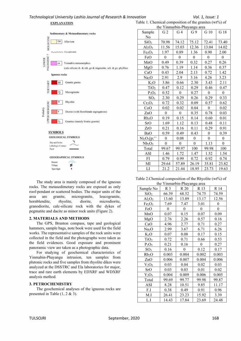
The study area is mainly composed of the igneous
rocks. The metasedimetary rocks are exposed as only
roof-pendant or scattered bodies. The major units of the
area are granite, microgranite, leucogranite,
hornblendite, rhyolite, diorite, microdiorite,
granodiorite, calc-silicate rock with the dykes of
pegmatite and dacite as minor rock units (Figure 2).
2. MATERIALS AND METHODS
The GPS, Brunton compass, tape and geological
hammers, sample bags, note book were used for the field
works. The representative samples of the rock units were
collected in the field and the photographs were taken as
the field evidences. Good exposure and prominent
panoramic view are taken as a photographic data.
For studying of geochemical characteristics of
Yinmabin-Phayangu intrusion, ten samples from
plutonic rocks and five samples from rhyolite dikes were
analyzed at the DSSTRC and Ela laboratories for major,
trace and rare earth elements by EDXRF and WDXRF
analysis method.
3. PETROCHEMISTRY
The geochemical analyses of the igneous rocks are
presented in Table (1, 2 & 3).
Table 1. Chemical composition of the granites (wt%) of
the Yinmarbin-Phayangu area
Sample
No
G 2 G 4 G 9 G 10 G 18
SiO2 70.98 74.12 75.12 72.41 73.40
Al2O3 11.56 15.03 12.36 13.04 14.02
Fe2O3 1.97 0.89 1.36 0.90 2.00
FeO 0 0 0 0 0
MnO 0.49 0.39 0.32 0.27 0.26
MgO 0.76 1.19 1.14 0.36 0.37
CaO 0.43 2.04 2.13 0.72 1.42
Na2O 2.91 2.9 3.16 4.26 3.23
K2O 3.86 0.66 2.30 3.43 2.11
TiO2 0.47 0.12 0.29 0.46 0.47
P2O5 0.52 0 0.27 0 0
SO3 2.30 0.29 0.26 0.29 0.33
Cr2O3 0.72 0.32 0.09 0.57 0.62
CoO 0.02 0.02 0.04 0 0.02
ZnO 0 0 0.35 0.78 0.03
Rb2O 0.19 0.15 0.14 0.60 0.01
SrO 1.69 1.12 0.13 0.48 0.11
ZrO 0.21 0.16 0.11 0.29 0.91
BaO 0.59 0.49 0.43 0 0.39
Ni2O3[p;’’ 0 0.08 0 0 0
Nb2O5 0 0 0 1.13 0
Total 99.67 99.97 100 99.98 100
ASI 1.46 1.72 1.47 1.52 1.54
FI 0.79 0.99 0.72 0.92 0.74
MI 29.64 57.89 26.19 35.81 23.82
LI 21.2 21.44 18.95 23.73 19.63
Table 2.Chemical composition of the Rhyolite (wt%) of
the Yinmarbin-Phayangu area
Sample No R 3 R 20 R 13 R 14
SiO2 66.39 68.52 74.75 74.59
Al2O3 13.60 13.89 13.17 12.56
Fe2O3 7.69 7.47 3.01 0
FeO 0 0 0 0
MnO 0.07 0.15 0.07 0.09
MgO 2.76 2.26 0.57 0.16
CaO 4.96 2.77 0.71 0.27
Na2O 2.99 3.67 6.71 6.26
K2O 0.07 0.08 0.17 0.15
TiO2 0.72 0.71 0.66 0.53
P2O5 0.21 0.16 0 0.27
SO3 0.16 0 0.12 0.17
Rb2O 0.003 0.004 0.002 0.003
ZnO 0.006 0.007 0.004 0.006
V2O5 0.03 0.04 0.02 0.03
SrO 0.03 0.03 0.01 0.02
Y2O3 0.004 0.009 0.006 0.005
Total 99.69 99.77 99.98 99.87
ASI 8.28 10.51 9.85 11.17
F.I 0.38 0.49 0.91 0.96
M.I 26.41 23.23 15.92 3.39
L.I 14.43 17.84 23.69 24.48

Technological University Lashio Journal of Research & Innovation Vol. 1, Issue: 1
TULSOJRI September, 2020 169
Table 3. Chemical composition of the diorites (wt%) of
the Yinmarbin-Phayangu area
Sample
No
D 9 D 28 D 15 D 1
SiO2 57.78 56.06 53.40 49.66
Al2O3 17.91 16.81 16.72 16.93
Fe2O3 10.67 10.83 8.23 7.91
FeO 0 0 0 0
MnO 0.21 0.17 0.12 0.71
MgO 4.81 25.62 9.41 5.76
CaO 4.12 5.89 7.29 8.93
Na2O 2.56 3.40 2.29 3.57
K2O 0.29 0.59 1.32 1.20
TiO2 0.43 0 0.31 4.43
P2O5 0.18 0.11 0 0.16
SO3 0.34 0 0.33 0.42
Rb2O 0.36 0.02 0.003 0.003
Cr2O3 0.006 0.03 0.005 0.007
ZnO 0.004 0.003 0 0.002
ZrO2 0.015 0.006 0.03 0.03
V2O5 0.019 0 0.002 0
SrO 0.09 0.002 0 0.001
Y2O3 0.002 0.003 0.001 0.001
Total 99.79 99.54 99.96 99.72
ASI 2.57 1.70 1.47 1.24
F.I 0.41 0.41 0.36 0.35
M.I 31.07 34.16 53.34 42.14
L.I 10.43 3.37 1.54 2.26
The analyzed rocks show a restricted range in
chemical composition. The concentration of SiO2 in the
hornblende granite are low SiO2 (65.85-69.90) and high
total iron (5.48-8.39) as compared to leucocratic
granites: SiO2 (73.89-77.74) and total iron (1.10-5.06).
The average values of Al2O3, TiO2, Na2O, K2O, CaO,
MgO and P2O5 of the granites are 12.49, 0.79, 4.48, 4.96,
1.02, 0.27 and 0.20 which are comparatively same as
Leucocratic granites: 12.19, 0.26, 3.60, 4.02, 0.71, 0.12
and 0.01 respectively.
In the total alkali versus silica (TAS) diagram, the
mafic rock (SiO2 content ranges from 56.6% to 68.90%
Na2O+K2O ranges from 5.01% to 10.14%) fall within the
field of diorite and granodiorite whereas the acidic rocks
(SiO2) content ranges from51.8% to 75.5%, Na2O+K2O
ranges from 8.02% to 11.28%) plot in the granite field
and granodiorite field.
Fig3. SiO2 versus Na2O+K2O diagram of igneous
rocks of the study area with field after Rickwood (1989)
in [7].
Based on K2O + Na2O versus SiO2 diagram and the
AFM triangular diagram, all rocks units of the
Yinmabin-Phayangu intrusion are calc-alkaline
character (Figure 3& 4).
Fig4. AFM diagram of igneous rocks of the study
area
At the SiO2 against K2O diagram, they are classified
as high potassium calc-alkaline rocks (Figure 5). Their
very low contents of CaO, MgO with Fe/Mg ratios and
AI values signify alkali affinity of these granites. These
magmatic rocks attained very high content of sodium and
iron as well as strongly depleted in alumina along with
calcium and magnesium in their final stages of magmatic
and subsolidus processes. So, it can be considered that
calc-alkaline nature of granitic rocks from the study area
is genetically related to the subduction related plate
tectonic process.
Fig5. SiO2 versus Na2O+K2O diagram of igneous
rocks of the study area with field after Rickwood (1989)
in [7].
The alumina situation index (ASI), defined as the
molecular A/ CNK= Al2O3/ CaO+ K2O+Na2O, ranges
from 1.83 to 1.97 for the granitic rocks. Shand (1927)
grouped igneous rocks based on the total molecular alkali

Technological University Lashio Journal of Research & Innovation Vol. 1, Issue: 1
TULSOJRI September, 2020 170
versus alumina content as either peralkaline [Al2O3<
(Na2O+K2O)] peraluminous [Al2O3> (CaO+Na2O=
+K2O)] or metaluminous [Al2O3< (CaO+Na2O+K2O] (in
Winter, 2013). Chemically, the granitic rocks from the
study area have alumina greater than the sum of lime,
soda and potash [Al2O3> (CaO+Na2O+K2O)]. In Al2O3-
CaO-(Na2O+K2O) diagram too all the granitic rocks fall
within the peraluminous field (Figure 6).
Fig6. Al2O3 – CaO – (Na2O+ K2O) diagram of
plutonic rocks.
On the variation diagrams (Figure 7), with
increasing SiO2, contents of Al2O3, P2O5, CaO, TiO2,
MgO, MnO and Fe2O3 are decreased and K2O and Na2O
demonstrate increasing trend. These trends may reflect
the crystal fractionation process in the evolution of the
Yinmabin-Phayangu intrusion.
Fig7. SiO2 versus major oxides (wt%) variation
plots of the plutonic rocks.
4. PETROGENESIS
Granitoid rocks have been classified as both I-type
and S-type [3]. Several evidences suggest that Yinmabin-
Phayangu intrusion is I-type and S-type:
-Frequency of hornblende, magnetite, biotite and
titanite in theses rocks and absence of muscovite, garnet,
cordierite, andalusite and sillimanite.
-SiO2 content varies between 56.5% - 74.75% in
these rocks.
-Presence of mafic dolerite enclaves in different
parts of the intrusion and the absence of micaceous
xenoliths.
- Some samples are metaluminous and some are
peraluminous nature of them.
- Commonly present of pegmatites and aplite.
- Decreasing P2O5 versus SiO2.
-Based on SiO2 vs. K2O the Yinmabin-Phayangu
intrusion classified as I-type and S-type granitoids.
Barbarin (1999) classified granitoids into 7 main
groups. Based on this classification, Yinmabin-
Phayangu intrusion is classified as amphibole-bearing
calc-alkaline granitoids (ACG) [4].
Based on geochemical studies, Yinmabin-Phayangu
granitoid can be classified as sodic granite (Na2O > K2O)
and has low values of Ni, Cr, Co and V. Lower contents
of these elements indicative for evolution of magma
during ascending and before complete crystallization.
The granitic magma from the study area might have
been generated at the liquidus temperature between
685˚C and 720˚C [5]. According to Khin Zaw (1990), the granitoid rocks
in Myanmar can be subdivided into three main N-S
trending belts viz. western belt, central belt and eastern
belt extended from Putao, Kachin State in the north
through Mogok, Mandalay to Tavoy and Mergui areas,
Tenasserim in the south over a distance of 1450 km. The
present study area, Yinmabin-Phayangazu area is located
in the central granitoid belt. The central belt granitoid
plutons contain both I-type and S-type. The almost
absence of cogenetic volcanic rocks and abundance of
pegmatites, aplites and related quartzo-feldspathic vein
materials suggest a relatively deeper environment of
emplacement.
The potash-rich nature of the granitoids combined
with high initial ratios of Sr86/Sr87 (0.717 + 0.002) and
Rb/Sr ratios of (0.40-33.07) with an average value of
6.70 suggest the derivation of the central belt granitoid
magma from well-established continental, sialic
materials perhaps by remelting of medium- to high-
grade, regionally metamorphosed country rocks.
The granitoid rocks in the central belt were possibly
emplaced during continent-arc collision at the early stage
of westward migrating, east-dipping subduction zone
Eocene. The W-Sn related, central belt granitoids and
porphyry Cu (Au) related, western belt granitoids were
considered to have been emplaced during the Upper
Mesozoic and Lower Cenozoic interval but might not
have been strictly contemporaneous.
The igneous complex, about 29 km long and 13 km wide,
is the southern extension of the Pyetkaywe batholith in
the north. Associated igneous rocks are diorites together
with hornblendites; rhyolites occurring both as lava
flows and dykes; hornblende granites, muscovite
granites, felsic granites and pegmatites as younger

Technological University Lashio Journal of Research & Innovation Vol. 1, Issue: 1
TULSOJRI September, 2020 171
intrusive. The Yinmabin granitoids are medium- to
coarse-grained, non-porphyritic to porphyritic biotite
granites.
As the study area is located in back-arc of Myanmar,
the igneous of the study area were originated by the
product of calc-alkaline suite produced from the partial
melting of the subducted oceanic crust of Indian Plate
beneath the Burma Plate [6].
The occurrence of muscovite in the highly
differentiated leucogranites in the central belt granitoids
is also indicative of the emplacement at a depth greater
than 2.5 km.
Fig8. Location of the studied samples on the AFM
diagram after Bowden (1984) in [4].
diagrams also demonstrate a subduction setting
relation for the Yinmabin-Phayangazu granitoids. With
reference to [4], the tectonic setting of plutonic rocks
from the study area has been treated. The studied rocks
located in the continental arc granites (CAG) setting
(Figure 8), indicating that these granitoids originated
from the subduction of an oceanic crust under a
continental crust at the active continental margins. The
parental magma was medium to high K calc-alkaline. In
Al2O3 vs SiO2 diagram (Figure 9), the plutonic rocks can
be subdivided into three groups (IAG+CAG+CCG,
RRG+CEUG and POG) and the plutonic rocks of the
study area plot within the fields of IAG+CAG+CCG. Based on the above mentioned data, all plutonic
rocks from the study area belong to the fields of CCG and CAG. It can be considered that the plutonic rocks of the study area were formed on the continent owing to the subduction of an oceanic plate beneath the continent.
Fig9. Al2O3 vs SiO2 diagram. Granites, rhyolites and
diorite from the study area plot in the IAC+CAG+CCG
field. IAG= Island arc granitoids, CAG= Continental arc
granitoids, CCG= Continental collision granitoids,
POG= Post orogenic granitoids, RRG= Rift related
granitoids and CEUG= Continental Epeirogenic uplift
granitoids) (The fields are based on [7]).
5. CONCLUSION
All the analyzed rocks show a restricted range in
chemical composition. Based on K2O + Na2O versus
SiO2 diagram and the AFM triangular diagram, all rocks
units of the Yinmabin-Phayangu intrusion are calc-
alkaline character. In Al2O3-CaO-(Na2O+K2O) diagram
too all the granitic rocks fall within the peraluminous
field. On the variation diagrams, with increasing SiO2,
contents of Al2O3, P2O5, CaO, TiO2, MgO, MnO and
Fe2O3 are decreased and K2O and Na2O demonstrate
increasing trend. Yinmabin-Phayangu intrusion is
classified as amphibole-bearing calc-alkaline granitoids.
Based on geochemical studies, Yinmabin-Phayangu
granitoid can be classified as sodic granite (Na2O > K2O)
and has low values of Ni, Cr, Co and V. The granitic
magma from the study area might have been generated at
the liquidus temperature between 685˚C and 720˚C. The occurrence of muscovite in the highly differentiated
leucogranites in the central belt granitoids is also
indicative of the emplacement at a depth greater than 2.5
km. All plutonic rocks from the study area belong to the
fields of CCG (Continental collision granitoids) and
CAG (Continental arc granitoids). It can be considered
that the plutonic rocks of the study area were formed on
the continent owing to the subduction of an oceanic plate
beneath the continent.
ACKNOWLEDGMENT
WE WOULD LIKE TO EXPRESS OUR HEARTFELT
GRATITUDE TO RECTOR (ACTING), DR. AUNG MYO THU,
OF TECHNOLOGY UNIVERSITY (MEIKTILA) AND DR. AUNG
CHAN WIN, PROFESSOR AND HEAD OF DEPARTMENT OF
CIVIL ENGINEERING, TECHNOLOGY UNIVERSITY
(MEIKTILA) FOR THEIR INTEREST AND ENCOURAGEMENT
ON OUR RESEARCH WORK.

Technological University Lashio Journal of Research & Innovation Vol. 1, Issue: 1
TULSOJRI September, 2020 172
REFERENCES
[1] Maung Thein, 1972. Proposal for stratigraphic,
Structural, Lithological symbols and Chronographic
colour for use in the Burmese Geological Maps:
paper read at 1972 Burma Research Congress on Dec,
31, 1972.
[2] Ei Ei Myo, 2014. Geology and Petrology of
Migmatities in Payangazu-Chauksu Taung and
Kanabaw Areas, Thazi and Pyawbwe Townships,
Mandalay Region. Unpublished MRes (Thesis). Department of Geology, University of Yangon.
[3] Khin Zaw, 1990. Geological, Petrology and
Geochemical characteristics of granitoid rocks in
Burma, with special reference to the associated of W-
Sn mineralization and their tectonic setting. Journal of Southeast Asia Each Science. Vol-4.
[4] R. Keshavarzi, D. Esmaili, M.R. Kahkhae, M.A. A.
Mokhtari, R. Jabari, “Petrology, Geochemistry and
Tectonomagmatic Setting of Neshveh Intrusion (NW
Saveh)”, Open Journal of Geology, 2014, 4, pp.177-
189
[5] Hein Min Htike, 2016. Petrology of Plutonic Rocks
exposed in Kywedatson Area, Tharzi Township,
Mandalay Region. Unpublished M.Sc (Thesis),
Department of Geology, Pakokkou University.
[6] Khin Zaw, 1998. Geological evolution of selected
granitic pegmatites in Myanmar (Burma); constraints
from Regional Setting, Lithology and fluid-inclusion
studies. International Geology review, 40:7, p647-
662.
[7] A.K. SINGH & R.K.B SINGH, “PETROGENETIC
EVOLUTION OF THE FELSIC AND MAFIC VOLCANIC
SUITE IN THE SIANG WINDOW OF EASTERN
HIMALAYA, NORTHEAST INDIA”, GEOSCIENCE
FRONITERS 3(5), 2012, PP 613-634.

Technological University Lashio Journal of Research & Innovation Vol. 1, Issue: 1
TULSOJRI September, 2020 173
GEOCHEMICAL CLASSIFICATION OF SANDSTONES OF CHAUK OIL FIELD IN
CHAUK TOWNSHIP, MAGWAY REGION
May Thu Aye(1), Dr.Pike Htwe(2), Kyi Myo Khaing(3)
(1) Department of Civil Engineering Technological University, Magway, Myanmar
(2) Associate Professor, Geology Department, Pakokku University, Myanmar (3) Department of Civil Engineering Technological University, Monywa, Myanmar
Email: [email protected]
ABSTRACT: The research area is situated on the
eastern bank of Ayeyarwaddy River, in Chauk
Township, Magway Region. It is bounded by latitudes N
20̊ 50ʹ 00ʺ and N 20 ̊ 55ʹ 00ʺ, longitude E 94 ̊48ʹ 00ʺ and E 94̊ 52ʹ 00ʺ in 2094-13 UTM Map. It is covered by the
Oligocene to Pliocene clastic sedimentary rocks. Among
them, Pyawbwe and Kyaukkok formations were studied
to predict the geochemical characteristics of the study
area. To conduct XRF analysis, six sandstone samples
were taken from the selected layer of sandstone in the
Pyawbwe Formation and six sandstones were taken from
the selected sandstone layers in the Kyaukkok
Formation. According to the chemical classification of
sandstone diagram, the sandstones of Pyawbwe and
Kyaukkok formations fall within the ‘Litharenite’.
KEYWORDS: River, rocks, Pyawbwe, Kyaukkok, sandstones, Litharenite.
1. INTRODUCTION
The study area, Chauk Oil Field, is situated on the
eastern bank of Ayeyarwaddy River, in Chauk
Township, Magway Region. Basin. It is bounded by
latitudes 20 ̊50ʹ 00ʺ and N 20 ̊55ʹ 00ʺ, longitude E 94̊ 48ʹ 00ʺ and E 94̊ 52ʹ 00ʺ in 2094-13 UTM Map (Fig 1).
Fig 1. Location map of Chauk Area
The present area is approximately 63 square
kilometer (24.1 square mile), 9 km (5.6 mile) long in
north-south direction, and 7 km (4.3 mile) wide in east-
west direction.
The present area is approximately 63 square
kilometer (24.1 and 7 km (4.3 mile) wide in east-west
direction.
2. TOPOGRAPHY
Topographically, the study area can roughly be said
as the rolling terrain topography and a range of small
hills is running NNW-SSE direction in the eastern part.
The highest point of the study area located at the
northeastern margin is about 180m above sea level. The
western part of the area is bounded by the Ayeyarwaddy
River flowing from NNE to SSW. Low land topography
is present in the western and central parts of the area (Fig
2).
Fig 2. Physicographic map of Chauk Area
3. METHODOLOGY
There are four types of laboratory work;
Microscopic analysis, XRF analysis, sieving analysis
and porosity analysis. The laboratory works include
sample preparation before analysis. All laboratory
analysis will be undertaken at chemical Laboratory of
Material Science Research Centre, Ela and Laboratory of
Geology Department in Magway University.
Microscopic analysis will be conducted to determine
the petrology of siliciclastic rocks. The sample
preparation for microscopic analysis generally will
follow the procedures described in high quality section-
making process of Miller (1988). Microscopic
identification can be done to characterize the
composition and sedimentary texture.

Technological University Lashio Journal of Research & Innovation Vol. 1, Issue: 1
TULSOJRI September, 2020 174
The X-ray Fluorescence (XRF) analysis conducted
to know the chemical composition of sandstone and to
classify the sandstone. The samples collected in the field
were performed chemical analysis as X-Ray
Fluorescence. This method is most widely used analysis
techniques in the application of quantitative major
element analysis, minor and trace element analysis
(Hutchison, 1974). Selected samples from the
mineralization of the research area were analyzed using
X-Ray fluorescence (XRF) for major oxides and some
trace elements. In this research-ray fluorescence (XRF)
analyses were be done to interpret the chemical
classification and weathering of the clastic sediments.
4. STRATIGRAPHY
The research area can be classified into four major
stratigraphic units such as (1) Okhmintaung Formation
of lower Pegu Group (2) Pyawbwe Formation, and (3)
Kyaukkok Formation of Upper Pegu Group and (4)
Irrawaddy Formation (Fig 3).
The late Oligocene strata are constituted mainly of
yellowish-brown colored, medium-grained sandstones
interbedded with the laminated shale. The Miocene
of Upper Pegu Group is yellowish-brown colored
sandstones and light-gray colored shale and fossiliferous
conglomerate band. Late Miocene-Pliocene Irrawaddy
Formation is characterized by buff color to yellowish grey,
thick-bedded to massive, unfossiliferous friable sandstones
which are widely exposed in the flank of the major anticline.
The stratigraphic succession and lithology of the Chauk area
are shown in Table (1).
Table 1. Stratigraphic succession of Chauk Area
Age Formation Lithology Thickness
Lat
e M
io-
Pli
oce
ne
Irrawaddy Formation
Yellowish brown to buff colored , medium to coarse -grained, massive sandstone with large scale cross-bedding and fossil wood
629m (Than
Htike Oo, 2012)
Mid
dle
Mio
cene
Kyaukkok Formation
Yellowish brown colored, medium to thick - bedded sandstone with concretion intercalated with shale
266m
Ear
ly
Mio
cene
Pyawbwe Formation
Light grey colored mudstone and sandstone with interformational conglomerate containing mud clasts
290m
Lat
e
Oli
goce
ne
Okhmintaung Formation
Yellowish grey colored , thick -bedded to massive sandstone with subordinate shale and fossiliferous conglomerate band
164m
Fig 3. Geological Map of Chauk Area
(Modified after M.O.G.E, 1980)
4.1 Okhmintaung Formation
This unit is composed of sandstone with minor
amount of conglomerate and thinly grey shale exposing
at Okhmintaung Ridge (N 19̊ 30̍, E 94̊ 54̍) NNW of
Thayet, Magway Region. The stratigraphic thickness in
type section is 3000 feet.
4.1.1 Distribution and Thickness
The Okhmintaung Formation generally occupies in
the core of Chauk Anticline, in the SE of Patamyataung
and near the Kyaukte village. The best exposure of this
formation is exposed along Kyaukte - Ohnmya road
section and east of Chauk. The thickness of
Okhmintaung Formation exposed in the present area is
164 m in the present study (Fig 4).
4.1.2 Lithology
The Okhmintaung Formation is composed of
medium to thick bedded sandstone intercalated with
shale beds and minor thin conglomerate beds. In the
study area, yellowish brown colored, fine to medium -
grained, medium to thick - bedded sandstone with mud
lamination and indurated sand (Fig 5). In the lower part

Technological University Lashio Journal of Research & Innovation Vol. 1, Issue: 1
TULSOJRI September, 2020 175
of this formation. In the upper part, the shale becomes
more frequent.
Fig 4. Stratigraphic column of Okhmintaung Formation
at Kyaukte Chaung section.
Fig 5. The alternation of light brown, medium bedded
sandstone and grey to bluish grey shale with gypsum
near the west gate of Kyaukte Village (N20̊ 54̍ 38̋, E 94̊ 50̍ 33̋ )
4.2 Pyawbwe Formation
The name of this formation was first introduced by
Lepper (1933) as “Pyawbwe Formation’’ which crops out near the Pyawbwe village (N 20 ̊ 01̍, E 94̊ 38̍) in
Minbu Township, Magway Region. It is typically about
600 meters thick. The Pyawbwe Formation was
previously called the Pyawbwe Clays.
Fig 6. Stratigraphic column of Pyawbwe Formation at
Kyaukte Chaung section.
4.2.1 Distribution and Thickness
In the study area, the Pyawbwe Formation exposed
both eastern and western flank of Chauk Anticline.
According to the asymmetrical nature of the anticline,
the exposure of the Pyawbwe Formation in the western
flank of major anticline may be wider than that of the
eastern flank. In the study area, the best exposure of this
formation is exposed near Kyaukte village and along the
railway section from Chauk to Tayawgon station. In
present study, the thickness of Pyawbwe Formation is
about 290 m in Kyaukte section (Fig 6).
4.2.2 Lithology
The Pyawbwe Formation consists mainly of pale
brown to bluish grey shale (Fig 7), grey sandy
concretionary shale with thin fossiliferous sandstone,
occasionally intercalated with indurated sandstone bands
and thin conglomerate band. In the upper part of this
formation, light brown to dark brown, fine to medium -
grained, medium to thickly - bedded, planner and
through cross bedding .
Fig 7. Pale brown to bluish grey shale lenticular
sand at the stream section near the east entrance of
Kyaukte Village (20̊ 54̍ 23 ̋,E 94̊ 49̍ 40 ̋ )
4.3 Kyaukkok Formation
The name of this formation was given by Lepper
(1933) as “Kyaukkok Formation’’ and exposed near the
Kyaukkok village (N19̊ 54 ̋, E94̊ 43 ̋ ) in the Minbu
District, Magway Region.
4.3.1 Distribution and Thickness
The Kyaukkok Formation is well exposed in both
flanks of the Major Anticline in the study area. This
formation is well cropped out around the Ayesayti
Pagoda Hill, Yankintaung (Aungmyay monastery) and
west of Chauk railway station. The exposed thickness of
this formation is different in places. Generally it was 266
m thick in the western flank of anticline (Fig 8).
4.3.2 Lithology
This formation is dominantly made up of brown to
buff colored, fine to medium - grained, medium to thick-
bedded sandstone with thin shale partings and sandstones
with calcareous concretions rich in fossils. Thinly to
medium - bedded, yellowish brown sandstone
interbedded with light grey shale are also found within
the Kyaukkok Formation (Fig 9). In the lower part of the
formation, medium - grained sandstones are more

Technological University Lashio Journal of Research & Innovation Vol. 1, Issue: 1
TULSOJRI September, 2020 176
common, and gradually coarser towards the upper part of
this unit.
Fig 8. Yellowish brown sandstone interbedded with
light grey shale (N 20˚ 53̍ 01 ̋ , E 94̊ 49̍ 57 ̋ )
Fig 9. Stratigraphic column of Kyaukkok Formation at
railway section in the western flank of anticline
4.4 Irrawaddy Formation
The term “Fossil Wood Group’’ was firstly used by Theobald (1873) to a sandy, gritty to pebbly sandstone
containing abundant silicified wood fossils which
overlies the Upper Pegu Group. Later, Noething (1900)
described the term “Irrawaddy Series’’ for the same lithostratigraphic unit.
4.4.1 Distribution and Thickness
The Irrawaddy Formation is well exposed in the
Pinmagon, near the Ayeyarwaddy Bridge in the western
flank of Chauk Anticline and near the Ohnmya village,
NE of Chauk in the eastern flank. This formation is
composed of brown to whitish color, coarse to gritty
sandstones, mottle clays and occasional pebbly
sandstones with silicified wood fossil.
4.4.2 Lithology
The sandstones of yellowish brown to buff colored,
massive to thick - bedded with large scale cross bedding
are mainly composed in Irrawaddy Formation of Chauk
area. Gritty sandstones with pebbly layers are dominant
in the lower part. The pebbles are ranging from ½ to 2
inches in diameter and they are well rounded and fairly
sorted. Silicified wood fossils are locally developed in
the lower part of this formation.
5. RESULT AND DISCUSSION
The Pyawbwe Formation and Kyaukkok Formation are generally exposed along North - South trending in the study area. A number of good outcrops are situated at both eastern and western flank of Chauk Anticline. Kyaukte stream section and the road section from Taywagon to Chauk are measured in the study area.
To conduct XRF analysis, six sandstone samples
were taken from the selected layer of sandstone in the
Pyawbwe Formation and six sandstones were taken from
the selected sandstone layers in the Kyaukkok
Formation.
The three samples (KP.36, KP.84, and KP.128) are
selected from the Pyawbwe Formation in Kyaukte
stream section and three samples (KP.11, KP.21, KP.34)
are selected from the Pyawbwe Formation in Tayawgon
railway station.
The three samples (NK 29, NK.60, and NK.95) are
taken in the Kyaukkok Formation cropped out in the
western flank of Anticline and (NK.19, NK 36, Nk.51)
are taken in the Kyaukkok Formation exposed in the
eastern flank of Anticline.
The geochemical compositiom (Wt%) of Pyawbwe Sandstone is shown in Table 2 and Table 3shows the log ratios of Log ratios of SiO2/Al2O3 and Na2O/K2O and Fe2O/K2O concentration (%) for Sandstone of Pyawbwe Formation.
The weight of geochemical composition (Wt%) of Kyaukkok Sandstone is shown in Table 4 and Table 5 shows Log ratios for SiO2/ Al2O3 and Na2O/K2O and Fe2O3/K2O concentration (%) for Sandstone in Kyaukkok Formation.
The classification schemes used are the geochemical
classification diagrams of Pettijohn et al, (1972).
Pettijohn et al, (1972) examined the importance of these
major oxide variables. The geochemical classification
diagram by Herron (1988) classifies them mainly as Fe-
sands with little portions on the wacke zone.
The result of log ratio are plotted on chemical
classification of sandstone of Pettijohn et al, (1972) and
Herron (1988). According to the chemical classification
of sandstone diagrams (Fig 10), the sandstone of
Pyawbwe Formation fall within the Litharenite.
The chemical classification of sandstone diagrams
(Fig 11), interpreted that the sandstone of Kyaukkok
Formation also fall within the litharenite zone. The
litharenite are in fluvial, deltatic environments associated
with active continental margins. The source area of these
lithic fragments are volcanism, thin-skinned faulting and
continental collisions.

Technological University Lashio Journal of Research & Innovation Vol. 1, Issue: 1
TULSOJRI September, 2020 177
Table 2. Oxide composition of sandstone in Pyawbwe
Formation
KP. 128 KP. 36 KP. 84 NP(W).
21
NP(W).
11
NP(W).
34
SiO2 70.09 72.4 73.44 68.11 69.82 74.36
Al2O3 10.26 9.1 6.84 8.19 10.24 9.48
Na2O 4.65 3.85 3.5 4.85 4.75 3.9
Fe2O3 5.98 4.98 5.35 6.57 5.99 4.95
CaO 3.01 3.93 - 3.34 2.93 2.97
K2O 2.92 2.97 2.58 2.97 2.95 2.88
TiO2 0.51 0.6 0.39 1.07 0.69 0.54
SO3 0.46 0.7 1.04 - 0.55 0.48
Cr2O3 0.07 0.17 0.16 0.47 0.13 0.02
MnO 0.21 0.31 3.39 0.53 0.27 0.07
V2O5 0.27 - 0.16 0.47 0.13 0.03
ZrO2 0.07 0.17 0.16 0.47 0.13 0.02
SrO 0.14 0.18 0.24 0.48 0.13 0.03
CuO 0.07 0.17 0.17 0.46 0.11 0.02
NiO 0.07 0.16 0.16 0.47 0.01 0.04
ZnO 0.064 0.18 0.153 0.48 0.14 0.02
Ag2O - - - - 0.11 -
Rb2O - 0.18 0.16 0.48 - 0.04
Y2O3 0.064 0.19 0.16 0.46 - -
Table 3. Log ratios of SiO2/Al2O3 and Na2O/K2O and
Fe2O/K2O concentration (%) for sandstone in Pyawbwe
Formation
SiO2 Al2O3 Na2
O K2O Fe2O3
Log
(SiO2/
Al2O3)
Log
(Na2O/
K2O)
Log
(Fe2O3/
K2O)
KP.128 70.09 10.26 4.65 2.92 5.98 0.83 0.2 0.31
KP.36 72.4 9.1 3.85 2.97 4.98 0.9 0.11 0.22
KP.84 73.44 6.84 3.5 2.58 5.35 1.05 0.31 0.31
NP(W)21 68.11 8.19 4.85 2.97 6.57 0.91 0.13 0.34
NP(W)11 69.82 10.24 4.75 2.95 5.99 0.83 0.2 0.3
NP(W)34 74.36 9.48 3.9 2.88 4.95 0.94 0.13 0.23
Table 4. Oxide composition of sandstones in Kyaukkok
Formation NK.29 NK.60 NK.95 NKe19 NKe36 NKe51
SiO2 72.68 70.68 72.03 72.83 69.35 73.29
Al2O3 9.04 9.52 8.34 7.63 10.69 7.6
Na2O 2.5 2.65 4.85 4.63 4.5 6.65
Fe2O3 4.5 4.08 4.24 4.47 6.49 5.97
CaO 2.98 3.34 3.47 2.89 3.03 2.97
K2O 1.69 1.83 2.11 2.83 2.83 2.91
TiO2 0.94 0.94 0.72 0.58 0.6 0.53
SO3 0.43 - 0.76 0.63 - -
Cr2O3 0.27 0.47 0.33 0.23 0.16 0.02
MnO 0.24 3.5 0.43 0.4 0.37 0.12
V2O5 0.19 0.46 0.33 0.24 0.16 0.02
ZrO2 0.18 0.47 0.32 0.23 0.16 0.03
SrO 0.18 0.46 0.34 0.26 0.17 0.03
CuO 0.16 0.45 0.32 0.22 0.143 0.02
NiO 0.16 - - - 0.15 0.01
ZnO 0.16 0.45 0.32 0.22 0.134 0.02
Ag2O - - 0.32 0.23 - -
Rb2O - - - 0.23 - -
Y2O3 - - - - 0.134 0.04
Table 5. Log ratios for SiO2/Al2O3 and Na2O/K2O and
Fe2O3/K2O concentration (%) for Sandstone in
Kyaukkok Formation
SiO2 Al2O3 Na2O K2O Fe2O3
Log
(SiO2/
Al2O3)
Log
(Na2O/
K2O)
Log
(Fe2O3/
K2O)
NK.29 72.68 9.04 2.5 1.69 4.5 0.905 0.17 0.42
NK.60 70.68 9.52 2.65 1.83 4.08 0.87 0.16 0.34
NK.95 72.03 8.34 4.85 2.11 4.24 0.93 0.36 0.3
Nke.19 72.83 7.63 4.63 2.83 4.47 0.97 0.21 0.19
Nke.36 69.35 10.69 4.5 2.83 6.49 0.81 0.2 0.36
Nke.51 73.29 7.6 6.65 2.91 5.97 0.98 0.35 0.31
Fig 10. Chemical classification of sandstone samples
from Pyawbwe Formation based on (a) log (SiO2/
Al2O3) vs.log (Na2O/K2O) diagram of Pettijohn et al. (1972), and (b) log (SiO2/Al2O3) vs.log (Fe2O3/K2O)
diagram of Herron (1988).
Fig 11. Chemical classification of sandstone samples
from Kyaukkok Formation based on (a) log (SiO2/
Al2O3) vs.log (Na2O/K2O) diagram of Pettijohn et al. (1972), and (b) log (SiO2/Al2O3) vs.log (Fe2O3/K2O)
diagram of Herron (1988).
6. CONCLUSIONS AND RECOMMENDATIONS
The composition of sandstone can be got from XRF
analysis. Sandstone is classified and named based on
their major oxides elements. The concentration of three
major oxide groups have been used to classify
sandstones; silica and alumina, alkali oxides, and iron
oxides plus magnesia.
Based on the chemical classification of sandstone
diagrams of Pettijohn et al, (1972), and of Herron (1988)
the sandstones of Pyawbwe and Kyaukkok formations
are litharenite sandstone. These sandstones are derived
from volcanism, thin-skinned faulting and continental
collisions. The depositional environments of litharenite
sandstones are fluvial and deltatic environments.
The feldspar composition of litharenite sandstone is
less than 25 percent. The Early to Middle Miocene
litharenite sandstones in Chauk Oil Field are mainly
composed of 65-75% quartz. Quartz is one of hard and
the most stable mineral. It is also high resistant to
weathering process. Therefore, the reservoir quality of

Technological University Lashio Journal of Research & Innovation Vol. 1, Issue: 1
TULSOJRI September, 2020 178
litharenite sandstones of Pyawbwe and Kyaukkok
formations may be fair to good.
ACKNOWLEDGEMENTS
I am greatly thankful to my supervisor, Dr. Khin
San, Professor (Head of Geology Department), Magway
University, her permission, supervision and for her
departmental facilitates.
The author would like to express Dr. Paike Htwe,
Associate Professor, Geology Department, Pakokku
University, for his reading and repairing and suggesting
of the manuscript and for his supervision throughout the
course of this study. Finally, I wish to thank to all
teachers in Geology Department, Magway University,
and my colleagues of the same department for their help
and encouragement throughout the course of this
research work.
REFERENCES
[1] Eames, F.E., 1951, ‘The Peguian System of Central
Burma’: Rec.Geol.Surv. India.V-91, pp . 2. [2] Lepper, G .W., 1933, ‘Geology of the oil bearing
regions of the Chindwin- Irrawaddy valley of Burma and of Assam-Arakan, Proc. World Petroleum Congress’, vol.1, p.15-25.
[3] MGS, 2014, Myanmar Geosciences Society, ‘Geological Map of Myanmar (2014)’, Scale 1:2,250,000.
[4] M.O.G.E, 1980, ‘Geological Map of Central Myanmar Basin’, Scale 1inch to 4 miles.
[5] Pettijohn, F. J, Potter, P. E., Siever, R., 1972, ‘Sand and Sandstones’; New York, Springer- Verlag.
[6] Herron, M. M, 1988, ‘Geochemical classification of terrigenous sands and shale from core or log data’: Journal of Sedimentary Petrology, 58, 820-829.
[7] Noethling. F., 1990, ‘The Miocene of Burma’, Verhandelingen der Koninkliijke Akademie van Wetenschappenerhandelingen, (2)7(2), 1-131,1 map.3 figs. Amsterdam
[8] Theoblad, 1873, ‘The Geology of Pegu’, Memoirs of the geological survey of India, 10 (2), p.189-359.
[9] Than Htike Oo, 2012, ‘Mechanical analysis of Kyaukkok Formation in Chauk Area Magway Region’, Unpublished MSc thesis, Magway University
[10] Miller, J., 1988, ‘Microscopic techniques: 1, Slices, slides, strains and peels: in Techniques in Sedimentary:’ Tucker, M, Eds, Blackwell Scientific Publications, Oxford, p.86-107.
[11] Hutchison C.S., 1974, ‘Laboratory Hand Book of Petrographic Techniques’

Technological University Lashio Journal of Research & Innovation Vol. 1, Issue: 1
TULSOJRI September, 2020 179
Stratigraphy and Geochemical Characteristic of Volcanic and Pyroclastic rocks in
Yedwet-Wetkyikan area, Kyaukpadaung Township, Mandalay Region
Kyi Myo Khaing (1), Hline Wint Wint Hmue (2), May Thu Aye(3)
(1)Technological University (Monywa), Myanmar
(2)Technological University (Lashio), Myanmar (3)Technological University (Magway), Myanmar
Email: [email protected]
[email protected] [email protected]
ABSTRACT: The investigated area is situated in the
Kyaukpadaung Township, Mandalay Region.
Physiographically, the study area is a low-land area
with high denudation hills, Kyaukpadaung Taung
(Gaungni Taung), Yedwet Taung, Wetkyikan Taung
trending NNW-SSE. The rocks exposed in this area
are volcanic rocks (silicified rhyolite and hornblende-
biotite dacite), pyroclastic rocks (rhyolitic tuff and
dacitic tuff), ferruginous conglomerates, mud pebbly
gritty sandstones, sandstones and mudstones of
Irrawaddy Formation. The age of these rocks probably
range from Late Miocene to Pliocene. Geochemical
data has been used to characterize the volcanic rocks
in the present area. These lava and pyroclastic,
rhyolites and dacites are plotted within the field of
low, medium, high K series. In classified diagram
Na2O+K2O vs SiO2 made between alkaline and sub
alkaline series, all samples fall in the field of tholeiitic
series.
KEYWORDS: volcanic rocks, irrawaddy formation, K series, sub alkaline series, tholeiitic series
1. INTRODUCTION
In the present area, clastic sediments of
considerable thickness and volcanic and volcaniclastic
rocks are exposed. These rocks range in age from late
Miocene to Recent. In the study area, the Irrawaddy
Formation is a unit of sedimentary rocks composed of
(coarse to gritty sandstones, mud pebbly sandstones,
intraformational conglomerates and tuffaceous
sandstones with silicified wood-fossils), about 2
furlongs NW of the Kyaukpadaung area. The
sandstones are reddish brown to dark colored, very
coarse-grained, highly jointed and very thick bedded.
Gritty sandstones with mud pebbles are dominant and
ferruginous in the lower part. The mud pebbles are 6
inches to 1 foot in diameter and they are greenish gray,
subrounded and poorly sorted. Intraformational
quartz pebbly conglomerates are locally present in this
lower part. They overlie the mud pebbly gritty
sandstones. The tuffaceous sandstones are medium to
coarse grained and very thick bedded. They are white
to ash-gray in color. Silicified wood-fossils are locally
developed in this formation of the study area.
1.1 Location of the Study
The study area is located in the Kyaukpadaung
Township, bounded by north latitudes 20°45'00"-
20°49'32" and east longitudes 95°04'40"-95°13'35". It
occupies parts of one inch topographic maps 84P/1
and 84P/5. The location of the study area is shown in
Fig.1.
Fig 1. Location map of the Kyaukpadaung area
The present area is about 11 miles long and 7.5
miles wide in east-west and north-south directions,
respectively, covering 70 square miles of fairly rugged
terrain because of high denudational hills. It is situated
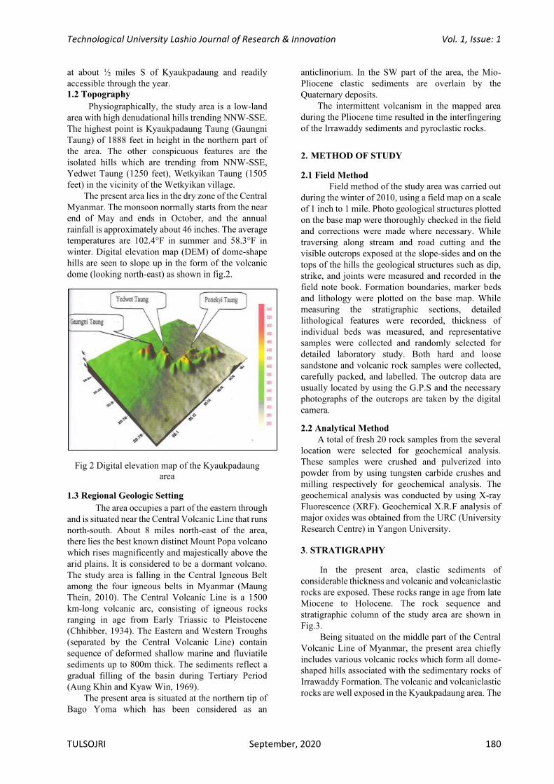
Technological University Lashio Journal of Research & Innovation Vol. 1, Issue: 1
TULSOJRI September, 2020 180
at about ½ miles S of Kyaukpadaung and readily
accessible through the year. 1.2 Topography
Physiographically, the study area is a low-land
area with high denudational hills trending NNW-SSE.
The highest point is Kyaukpadaung Taung (Gaungni
Taung) of 1888 feet in height in the northern part of
the area. The other conspicuous features are the
isolated hills which are trending from NNW-SSE,
Yedwet Taung (1250 feet), Wetkyikan Taung (1505
feet) in the vicinity of the Wetkyikan village.
The present area lies in the dry zone of the Central
Myanmar. The monsoon normally starts from the near
end of May and ends in October, and the annual
rainfall is approximately about 46 inches. The average
temperatures are 102.4°F in summer and 58.3°F in
winter. Digital elevation map (DEM) of dome-shape
hills are seen to slope up in the form of the volcanic
dome (looking north-east) as shown in fig.2.
Fig 2 Digital elevation map of the Kyaukpadaung area
1.3 Regional Geologic Setting
The area occupies a part of the eastern through
and is situated near the Central Volcanic Line that runs
north-south. About 8 miles north-east of the area,
there lies the best known distinct Mount Popa volcano
which rises magnificently and majestically above the
arid plains. It is considered to be a dormant volcano.
The study area is falling in the Central Igneous Belt
among the four igneous belts in Myanmar (Maung
Thein, 2010). The Central Volcanic Line is a 1500
km-long volcanic arc, consisting of igneous rocks
ranging in age from Early Triassic to Pleistocene
(Chhibber, 1934). The Eastern and Western Troughs
(separated by the Central Volcanic Line) contain
sequence of deformed shallow marine and fluviatile
sediments up to 800m thick. The sediments reflect a
gradual filling of the basin during Tertiary Period
(Aung Khin and Kyaw Win, 1969).
The present area is situated at the northern tip of
Bago Yoma which has been considered as an
anticlinorium. In the SW part of the area, the Mio-
Pliocene clastic sediments are overlain by the
Quaternary deposits.
The intermittent volcanism in the mapped area
during the Pliocene time resulted in the interfingering
of the Irrawaddy sediments and pyroclastic rocks.
2. METHOD OF STUDY
2.1 Field Method
Field method of the study area was carried out
during the winter of 2010, using a field map on a scale
of 1 inch to 1 mile. Photo geological structures plotted
on the base map were thoroughly checked in the field
and corrections were made where necessary. While
traversing along stream and road cutting and the
visible outcrops exposed at the slope-sides and on the
tops of the hills the geological structures such as dip,
strike, and joints were measured and recorded in the
field note book. Formation boundaries, marker beds
and lithology were plotted on the base map. While
measuring the stratigraphic sections, detailed
lithological features were recorded, thickness of
individual beds was measured, and representative
samples were collected and randomly selected for
detailed laboratory study. Both hard and loose
sandstone and volcanic rock samples were collected,
carefully packed, and labelled. The outcrop data are
usually located by using the G.P.S and the necessary
photographs of the outcrops are taken by the digital
camera.
2.2 Analytical Method A total of fresh 20 rock samples from the several
location were selected for geochemical analysis.
These samples were crushed and pulverized into
powder from by using tungsten carbide crushes and
milling respectively for geochemical analysis. The
geochemical analysis was conducted by using X-ray
Fluorescence (XRF). Geochemical X.R.F analysis of
major oxides was obtained from the URC (University
Research Centre) in Yangon University.
3. STRATIGRAPHY
In the present area, clastic sediments of
considerable thickness and volcanic and volcaniclastic
rocks are exposed. These rocks range in age from late
Miocene to Holocene. The rock sequence and
stratigraphic column of the study area are shown in
Fig.3.
Being situated on the middle part of the Central
Volcanic Line of Myanmar, the present area chiefly
includes various volcanic rocks which form all dome-
shaped hills associated with the sedimentary rocks of
Irrawaddy Formation. The volcanic and volcaniclastic
rocks are well exposed in the Kyaukpadaung area. The
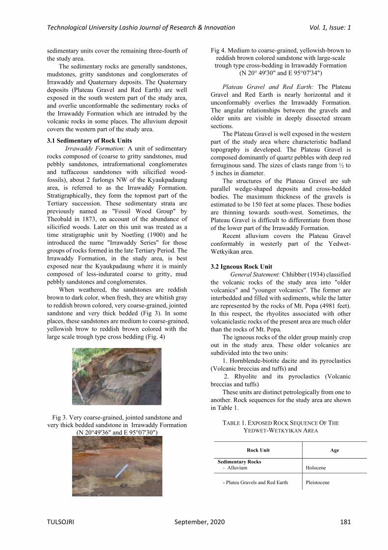
Technological University Lashio Journal of Research & Innovation Vol. 1, Issue: 1
TULSOJRI September, 2020 181
sedimentary units cover the remaining three-fourth of
the study area.
The sedimentary rocks are generally sandstones,
mudstones, gritty sandstones and conglomerates of
Irrawaddy and Quaternary deposits. The Quaternary
deposits (Plateau Gravel and Red Earth) are well
exposed in the south western part of the study area,
and overlie unconformable the sedimentary rocks of
the Irrawaddy Formation which are intruded by the
volcanic rocks in some places. The alluvium deposit
covers the western part of the study area.
3.1 Sedimentary of Rock Units
Irrawaddy Formation: A unit of sedimentary
rocks composed of (coarse to gritty sandstones, mud
pebbly sandstones, intraformational conglomerates
and tuffaceous sandstones with silicified wood-
fossils), about 2 furlongs NW of the Kyaukpadaung
area, is referred to as the Irrawaddy Formation.
Stratigraphically, they form the topmost part of the
Tertiary succession. These sedimentary strata are
previously named as "Fossil Wood Group" by
Theobald in 1873, on account of the abundance of
silicified woods. Later on this unit was treated as a
time stratigraphic unit by Noetling (1900) and he
introduced the name "Irrawaddy Series" for those
groups of rocks formed in the late Tertiary Period. The
Irrawaddy Formation, in the study area, is best
exposed near the Kyaukpadaung where it is mainly
composed of less-indurated coarse to gritty, mud
pebbly sandstones and conglomerates.
When weathered, the sandstones are reddish
brown to dark color, when fresh, they are whitish gray
to reddish brown colored, very coarse-grained, jointed
sandstone and very thick bedded (Fig 3). In some
places, these sandstones are medium to coarse-grained,
yellowish brow to reddish brown colored with the
large scale trough type cross bedding (Fig. 4)
Fig 3. Very coarse-grained, jointed sandstone and very thick bedded sandstone in Irrawaddy Formation
(N 20°49'36" and E 95°07'30")
Fig 4. Medium to coarse-grained, yellowish-brown to reddish brown colored sandstone with large-scale trough type cross-bedding in Irrawaddy Formation
(N 20° 49'30" and E 95°07'34")
Plateau Gravel and Red Earth: The Plateau
Gravel and Red Earth is nearly horizontal and it
unconformably overlies the Irrawaddy Formation.
The angular relationships between the gravels and
older units are visible in deeply dissected stream
sections.
The Plateau Gravel is well exposed in the western
part of the study area where characteristic badland
topography is developed. The Plateau Gravel is
composed dominantly of quartz pebbles with deep red
ferruginous sand. The sizes of clasts range from ½ to
5 inches in diameter.
The structures of the Plateau Gravel are sub
parallel wedge-shaped deposits and cross-bedded
bodies. The maximum thickness of the gravels is
estimated to be 150 feet at some places. These bodies
are thinning towards south-west. Sometimes, the
Plateau Gravel is difficult to differentiate from those
of the lower part of the Irrawaddy Formation.
Recent alluvium covers the Plateau Gravel
conformably in westerly part of the Yedwet-
Wetkyikan area.
3.2 Igneous Rock Unit
General Statement: Chhibber (1934) classified
the volcanic rocks of the study area into "older
volcanics" and "younger volcanics". The former are
interbedded and filled with sediments, while the latter
are represented by the rocks of Mt. Popa (4981 feet).
In this respect, the rhyolites associated with other
volcaniclastic rocks of the present area are much older
than the rocks of Mt. Popa.
The igneous rocks of the older group mainly crop
out in the study area. These older volcanics are
subdivided into the two units:
1. Hornblende-biotite dacite and its pyroclastics
(Volcanic breccias and tuffs) and
2. Rhyolite and its pyroclastics (Volcanic
breccias and tuffs)
These units are distinct petrologically from one to
another. Rock sequences for the study area are shown
in Table 1.
TABLE 1. EXPOSED ROCK SEQUENCE OF THE
YEDWET-WETKYIKAN AREA
Rock Unit Age
Sedimentary Rocks
- Alluvium Holocene
- Plateu Gravels and Red Earth
Pleistocene

Technological University Lashio Journal of Research & Innovation Vol. 1, Issue: 1
TULSOJRI September, 2020 182
- Irrawady Formation Late Miocene – Pliocene
Igneous Rocks -Hornblende-biotite dacite and its pyroclastics (Volcanic breccia & tuffs)
Late Miocene - Pliocene
- Rhyolite and its pyroclastics (Volcanic breccia & tuffs)
Rhyolite and its pyroclastics (Volcanic breccias and tuffs): These volcanic rocks occur as the blocky
lavas and occasional silicified lava domes. They are
white, grey or light yellow in color and usually form
small hillocks. All of the hills, such as Kyaukpadaung
Taung or Gaungni, Yedwet Taung, and Wetkyikan
Taung are built up of rhyolite and its pyroclastics
(volcanic breccias & tuffs).
The units form fine-grained, reddish brown,
holocrystalline rock with the phenocrysts of quartz
and feldspar. The rhyolites of the hills commonly
occupy the western slopes of the hills and the
pyroclastic rocks, the eastern slopes of the hills.
At the east side of the Wetkyikkan Taung, the
rhyolitic tuffs may be intruded by the quartz vein. In
some places, the joint planes of the tuffs are oxidized
and caused by the alteration of the mafic minerals in
these tuffs (Fig.5).
At the west of the Wetkyikan Taung, the tuffs are
found associated with the volcanic breccias,
constituted of the pebbles of the tuffs and silicified
rhyolites (Fig.6).
Fig 5. The joint planes of the tuffs of the mafic minerals in the rhyolitic tuffs (N 20°47'19" and E
95°10'52")
Fig 6. The tuffs associated with the volcanic breccia, constituted of the pebble of the tuff and silicified
rhyolites at the west of Wetkyikan Taung (N 20°47' 32" and E 95°10'27")
The Gaungni Taung is a dome-shaped hill made
up of silica-rich lava. At the base of Gaungni Taung
the silicified rhyolites are found as the scattered
blocks and irregular bodies. Some rhyolites may be
altered to ironstones due to the oxidation along their
joint planes (Fig.7).
At the middle part of the Gaungdi Taung, the
volcanic breccias about 15 feet in thickness are
associated with the silicified rhyolites and tuffs (Fig.8).
Fig 7. Rhyolite altered to ironstones due to the
oxidation along their joint planes (N 20°49'10" and E 95°08'11")
Fig 8. Volcanic breccias about 15 feet in thickness associated with silicified rhyolite and tuff at Gaungni hill (N 20°40'06"and E 95° 08' 13")
Biotite dacite and its pyroclastics: North of the
Wetkyikan village, about 2 forlongs occur as the
scattered blocks and dykes of the shallow type with
trending N-E. They may be considered to have
intruded after complete sedimentation of Irrawaddy
Formation and intrusion of rhyolite and its
pyroclastics. In this place, the layer deposits of tuffs
may probably be intruded by the later-formed dacite
dykes, because of the presence of tuff xenoliths are
formed within the dacites (Fig.9 & 10).
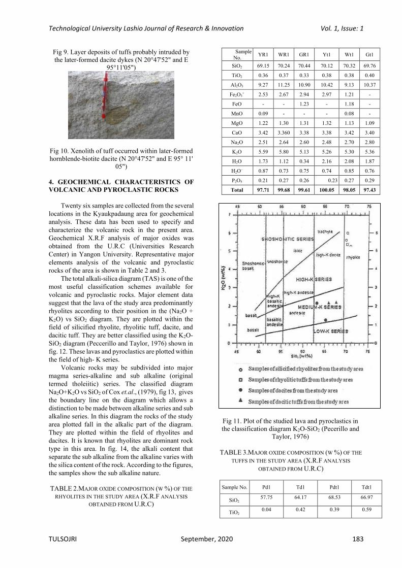
Technological University Lashio Journal of Research & Innovation Vol. 1, Issue: 1
TULSOJRI September, 2020 183
Fig 9. Layer deposits of tuffs probably intruded by the later-formed dacite dykes (N 20°47'52" and E
95°11'05")
Fig 10. Xenolith of tuff occurred within later-formed hornblende-biotite dacite (N 20°47'52" and E 95° 11'
05")
4. GEOCHEMICAL CHARACTERISTICS OF
VOLCANIC AND PYROCLASTIC ROCKS
Twenty six samples are collected from the several
locations in the Kyaukpadaung area for geochemical
analysis. These data has been used to specify and
characterize the volcanic rock in the present area.
Geochemical X.R.F analysis of major oxides was
obtained from the U.R.C (Universities Research
Center) in Yangon University. Representative major
elements analysis of the volcanic and pyroclastic
rocks of the area is shown in Table 2 and 3.
The total alkali-silica diagram (TAS) is one of the
most useful classification schemes available for
volcanic and pyroclastic rocks. Major element data
suggest that the lava of the study area predominantly
rhyolites according to their position in the (Na2O +
K2O) vs SiO2 diagram. They are plotted within the
field of silicified rhyolite, rhyolitic tuff, dacite, and
dacitic tuff. They are better classified using the K2O-
SiO2 diagram (Peccerillo and Taylor, 1976) shown in
fig. 12. These lavas and pyroclastics are plotted within
the field of high- K series.
Volcanic rocks may be subdivided into major
magma series-alkaline and sub alkaline (original
termed tholeiitic) series. The classified diagram
Na2O+K2O vs SiO2 of Cox et.al., (1979), fig 13, gives
the boundary line on the diagram which allows a
distinction to be made between alkaline series and sub
alkaline series. In this diagram the rocks of the study
area plotted fall in the alkalic part of the diagram.
They are plotted within the field of rhyolites and
dacites. It is known that rhyolites are dominant rock
type in this area. In fig. 14, the alkali content that
separate the sub alkaline from the alkaline varies with
the silica content of the rock. According to the figures,
the samples show the sub alkaline nature. TABLE 2.MAJOR OXIDE COMPOSITION (W %) OF THE
RHYOLITES IN THE STUDY AREA (X.R.F ANALYSIS
OBTAINED FROM U.R.C)
Sample No.
YR1 WR1 GR1 Yt1 Wt1 Gt1
SiO2 69.15 70.24 70.44 70.12 70.32 69.76
TiO2 0.36 0.37 0.33 0.38 0.38 0.40
Al2O3 9.27 11.25 10.90 10.42 9.13 10.37
Fe2O3+ 2.53 2.67 2.94 2.97 1.21 -
FeO - - 1.23 - 1.18 -
MnO 0.09 - - - 0.08 -
MgO 1.22 1.30 1.31 1.32 1.13 1.09
CaO 3.42 3.360 3.38 3.38 3.42 3.40
Na2O 2.51 2.64 2.60 2.48 2.70 2.80
K2O 5.59 5.80 5.13 5.26 5.30 5.36
H2O 1.73 1.12 0.34 2.16 2.08 1.87
H2O– 0.87 0.73 0.75 0.74 0.85 0.76
P2O5 0.21 0.27 0.26 0.23 0.27 0.29
Total 97.71 99.68 99.61 100.05 98.05 97.43
Fig 11. Plot of the studied lava and pyroclastics in the classification diagram K2O-SiO2 (Pecerillo and
Taylor, 1976)
TABLE 3.MAJOR OXIDE COMPOSITION (W %) OF THE
TUFFS IN THE STUDY AREA (X.R.F ANALYSIS
OBTAINED FROM U.R.C)
Sample No. Pd1 Td1 Pdt1 Tdt1
SiO2 57.75 64.17 68.53 66.97
TiO2 0.04 0.42 0.39 0.59

Technological University Lashio Journal of Research & Innovation Vol. 1, Issue: 1
TULSOJRI September, 2020 184
Al2O3 13.61 14.26 10.94 10.40
Fe2O3+
1.67 2.29 3.30 3.41
FeO 3.74 1.04 - 1.68
MnO 0.09 - - 0.09
MgO 1.51 1.32 1.35 1.81
CaO 5.43 5.39 5.38 6.95
Na2O 3.36 3.67 3.39 3.63
K2O 2.34 1.47 2.94 2.85
H2O 2.70 1.18 2.98 1.20
H2O– 1.05 0.81 1.09 0.79
P2O5 0.30 0.25 0.32 0.15
Total 99.55 97.27 100.61 99.82
Fig 12. Plot of the studied lavas and pyroclastics in the classification diagram Na2O+K2O vs SiO2(Cox
et. al., 1979)
Fig 13. Plot of the studied lavas and pyroclastics in the classification diagram Na2O+K2O vs SiO2
diagram separating the tholeiitic series (After Kuno, 1966)
4. CONCLUSIONS
In the present area, clastic sediments of
considerable thickness, volcanic and volcaniclastic
rocks are exposed. These rocks range in age from Late
Miocene to Pliocene. In the study area, the Irrawaddy
Formation is a unit of sedimentary rocks composed of
(coarse to gritty sandstones, mud pebble sandstones,
conglomerates and tuffaceous sandstones with
silicified wood fossils) about 2 furlongs NW of the
Kyaukpadaung area.
The igneous rocks of the older group mainly crop
out in the study area. These older volcanics are
subdivided into two units: (2) Hornblende-biotite
dacite and its pyroclastics (Volcanic breccias and
tuffs), (1) Rhyolite and its pyroclastics (Volcanic
breccias and tuffs).
Geochemical data has been used to characterize
the volcanic rock in the present area. Geochemical
X.R.F analysis of major oxide was obtained from the
U.R.C in Yangon University. They are better
classified using K2O+SiO2 diagram (Peccerillo and
Taylor, 1976). These lava and pyroclastic rocks are
plotted within the field low, medium, high K series. In
classified diagram Na2O +K2O vs SiO2 of Cox
et.al.(1979) made between alkaline series and sub
alkaline series, the rock of the study area plotted fall
in the sub alkaline part of the diagram. They are
plotted within the field of rhyolites and dacites. In the
Na2O + K2O vs SiO2 diagram. All samples fall in the
field of tholeiitic series. In Na2O + K2O vs SiO2
diagram (Irvine & Baragar, 1971) the sample show the
sub alkaline nature.
Technological University Lashio Journal of Research & Innovation Vol. 1, Issue: 1
TULSOJRI September, 2020 185
ACKNOWLEDGEMENT
I would like to express deep gratitude to U Myint
Zaw Han (Head of Department of Geology,
University of Magway, Retired) for valuable
suggestions, systematic guidance of the research work.
REFERENCES
[1] Aung Khin and Kyaw Win, “Preliminary studies
of the paleogeography of Burma during the
Cenozoic”. Union of Burma Journal. Sci. & Tech.
Vol.1.no.2. pp. 241-251.1969.
[2] Chhibber, H. L. “The Geology of
Burma. Macmillan London”.1934. [3] Cox, K.G., Bell J.D. and Pankhunst,
R.J, “The interpretation of igneous rocks”. London: Alen un win.1979.
[4] Irvin, T.N., Baragar, W.R.A., “A guide to
chemical classification of common volcanic
rocks”. Canadian Journal of Earth Sciences. 8.
pp.211- 218.1971.
[5] Maung Thein, “A preliminary syntaxsis
of the geological evolution of Burma with
reference to the tectonic development of
Southeast Asia”. Geological Society of Malaysia Bulletin. 6, pp. 87-116.2010.
[6] Neotling, F. “The Miocene of Burma: Mem”. Geol. Surv. India, Vii, pp. 2.1900.
[7] Peccerillo, A. and Tayer, S.R,
“Geochemistry of Eocene cal-alkaline volcanic
rocks from the Kustamanu Area, northern
Turkey, Contrib”. Mineral Petro. 58, p. 63-
81.1976.
[8] Theobald, W. “The Geology of Pegu, Memoirs of the geological survey of India”. 10(2). pp. 224- 302. 1873.
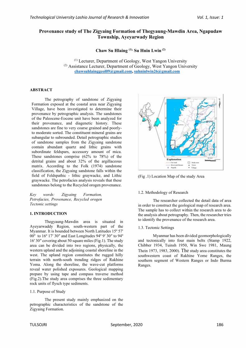
Technological University Lashio Journal of Research & Innovation Vol. 1, Issue: 1
TULSOJRI September, 2020 186
Provenance study of The Zigyaing Formation of Thegyaung-Mawdin Area, Ngapudaw
Township, Ayeyarwady Region
Chaw Su Hlaing (1), Su Hnin Lwin (2)
(1) Lecturer, Department of Geology, West Yangon University (2) Assistance Lecturer, Department of Geology, West Yangon University
[email protected], [email protected]
ABSTRACT
The petrography of sandstone of Zigyaing Formation exposed at the coastal area near Zigyaing Village, have been investigated to determine their provenance by petrographic analysis. The sandstones of the Paleocene-Eocene unit have been analyzed for their provenance, and diagenetic history. These sandstones are fine to very coarse grained and poorly- to moderate sorted. The constituent mineral grains are subangular to subrounded. Detail petrographic studies of sandstone samples from the Zigyaing sandstone contain abundant quartz and lithic grains with subordinate feldspars, accessory amount of mica. These sandstones comprise (62% to 78%) of the detrital grains and about 32% of the argillaceous matrix. According to the Folk (1974) sandstone classification, the Zigyaing sandstone falls within the field of Feldspathic - lithic graywacke, and Lithic graywacke. The petrofacies analysis reveals that these sandstones belong to the Recycled orogen provenance.
Key words: Zigyaing Formation, Petrofacies, Provenance, Recycled orogen Tectonic settings 1. INTRODUCTION
Thegyaung-Mawdin area is situated in Ayeyarwaddy Region, south-western part of the Myanmar. It is bounded between North Latitudes 15º 57' 00'' to 16º 17′ 30″ and East Longitudes 94º 9′ 30″ to 94º 16′ 30″ covering about 50 square miles (Fig.1). The study area can be divided into two regions, physically, the western upland and the adjoining coastal shoreline in the west. The upland region constitutes the rugged hilly terrain with north-south trending ridges of Rakhine Yoma. Along the shoreline, the wave-cut platforms reveal water polished exposures. Geological mapping prepare by using tape and compass traverse method (Fig.2).The study area comprises the three sedimentary rock units of flysch type sediments.
1.1. Purpose of Study
The present study mainly emphasized on the petrographic characteristics of the sandstone of the Zigyaing Formation.
(Fig .1) Location Map of the study Area
1.2. Methodology of Research
The researcher collected the detail data of area in order to construct the geological map of research area. The sample has to collect within the research area to do the analysis about petrography. Then, the researcher tries to identify the provenance of the research area.
1.3. Tectonic Settings
Myanmar has been divided geomorphologically and tectonically into four main belts (Stamp 1922, Chibber 1934, Tuinsh 1950, Win Swe 1981, Maung
Thein 1973, 1983, 2000). The study area constitutes the
southwestern coast of Rakhine Yome Ranges, the southern segment of Western Ranges or Indo Burma Ranges.

Technological University Lashio Journal of Research & Innovation Vol. 1, Issue: 1
TULSOJRI September, 2020 187
(Fig .2) Geological map of the study area (Modified from Paw Tun 1974)
2. RESULT AND DISCUSSION
Petrographic Study
Representative sandstones samples were collected from the Kwingu Formation, Zigyaing Formation, and Mawdin Formation exposing along coastal of Thegyaung-Mawdin area. Among them selected thin sections were prepared and examined under polarizing microscope for petrology and provenance analysis of Zigyaing sandstones. Fairly detailed point counts of Lithic grains as well as standard QFL % plotted on triangular classification scheme of Folk (1974) is utilizing for classification purpose. A total of 400 framework grains were identified per thin section for QFL mode and lithic population at spacing of 0.33mm.
2.1 Petrography of the Sandstones of Zigyaing
Formation
Microscopically, Zigyaing sandstones constitute 62% to 78% of detrital grains and about 32% of matrix to the total rock volume. These sandstones are generally medium to coarse grained, light grey to grey colored and are mainly comprised of quartz, feldspar, mica and rock fragments, and minor accessories minerals. Various types of grain to grain contacts such as point, long, tangential and concavo-convex contact are observed in sandstones of Zigyaing Formation. The detrital elements are embedded in the argillaceous matrix. The maximum grains size varies from 0.3mm to 0.8 mm in diameter and the minimum grain size varies from 0.05mm to 0.45mm in diameter.
Quartz
In the Zigyaing sandstones, quartz is abundant detrital mineral. Detrital quartz grains, both monocrystalline and polycrystalline, which comprise about 25% to 40% of total detrital fractions (Fig.5, 6). Most of monocrystalline quartz grains are sub-angular to sub-round and sub-sequent to sub-elongate in shape. Nearly 4% to 10% of the monocrystalline quartz grains show undulatory extinction and some grains show wavy extinction. A few polycrystalline quartz grains of igneous derivation and metamorphic derivations are present. The maximum grains size varies from 0.2mm to 0.4 mm in diameter and the minimum grain size varies from 0.05mm to 0.15mm in diameter.
Feldspar
Plagioclase and orthoclase feldspar grains consist about 15% to 25% of the total detrital fractions. Plagioclase feldspars are more common than orthoclase feldspar. Plagioclase feldspar is more than 80% of the total feldspar and some are slightly altered and found as dusty, cloudy or brown colored appearances in PPL. The size of feldspar ranges from 0.5 to0.85 mm in diameter. Most of plagioclase twin bands are distinct (Fig.7, 8). The maximum grains size varies from 0.05mm to 0.2 mm in diameter and the minimum grain size varies from 0.03mm to 0.07mm in diameter.
Mica
In the Zigyaing sandstones, biotite and muscovite are fairly common detrital fraction ranging from about 1% to 3 % of total detrital fractions are micas, in which biotite is much more dominate. Both biotite and muscovite are distorted by grain to grain compaction (Fig.8).Trace amounts of muscovite occur as flakes in the studied samples. They show bending due to deformation. In addition to muscovite, biotite also occurs. However, it mostly appears to be irregularly bifurcated due to the effect of compaction processes. Biotites are identified by its brown color under plane polarized light and strong pleochroism.
Rock Fragments
The rock fragments comprise about 20% to 30% of the total detrital fractions. Igneous rock fragments consists 10% to18% of the total rock fragments. Sedimentary rock fragments including fine-grained sandstone, shale and chert are present (Fig.9), which is more than metamorphic rock fragments but less than igneous rock fragments (Fig.10, 11, 12, 13, and 14). Metamorphic rock fragments comprise, averaging above 1% to 3% of the total rock fragment content including schist. The maximum grains size varies from 0.2mm to 0.6mm in diameter and the minimum grain size varies from 0.03mm to 0.15mm in diameter.
Cement and Matrix
In Zigyaing sandstones, the matrix is more than cement. Calcite cement and iron oxide cement are present in the sandstones of Zigyaing Formation. The detrital grains are well cemented by calcite. Hematite is

Technological University Lashio Journal of Research & Innovation Vol. 1, Issue: 1
TULSOJRI September, 2020 188
mostly common iron oxide cement which may show typical blood red color strong transmitted light. This is a characteristic of primary cementation before calcite precipitation. In argillaceous matrix, white mica or micaceous clays and chlorite, some carbonates, fine chips of quartz, feldspar from silty sizes to rock flour are essentially composed as the matrix materials.
Nomenclature of Zigyaing Sandstone
According to the sandstone classification of Folk (1974), most of the Zigyaing sandstones fall in the field of “Feldspathic Lithic graywacke” and “Lithic graywacke” (Fig. 4).
(Fig. 4)Ternary compositional Diagram ( Q-F-L% plot) of sandstones from Zigyaing Formation, Southwestern part of Rakhine Yoma, ( After Folk’s (1974).
(Fig.6) Polycrystalline quartz, igneous rock
fragment, plagioclase feldspar of Zigyaing
Formation(Under XN)
(Fig.8) Photomicrograph showing the
monocrystalline quartz (Qm), orthoclase
feldspar (or), plagioclase feldspar (pl), and
biotite mica (bm) of the Zigiaing Formation
(Under X.N).
(Fig.5) Photomicrograph showing the
monocrysstalline quartz, sedimentary rock
fragment, igneous rock fragment and
plagioclase feldspar (Under XN)
(Fig.7) Photomicrograph showing the albite
(multiple twinning) of plagioclase, sedimentary
rock fragment, monocrystalline quartz and
igneous fragment (Under XN)
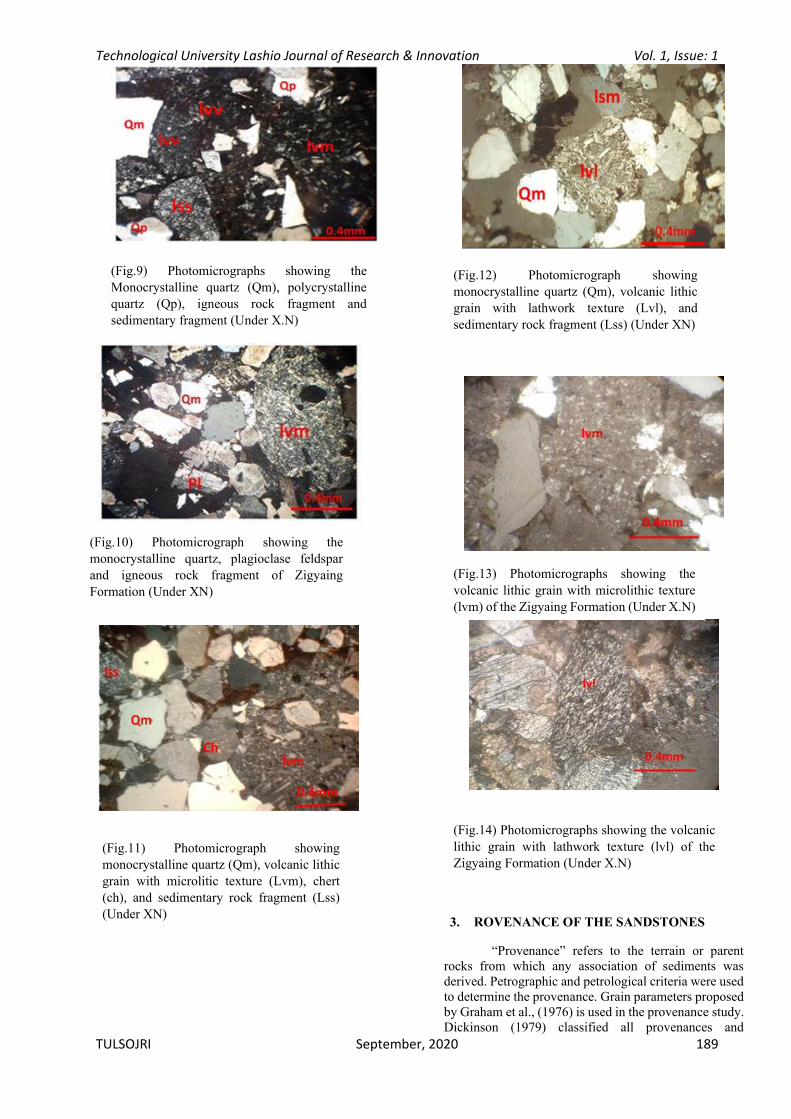
Technological University Lashio Journal of Research & Innovation Vol. 1, Issue: 1
TULSOJRI September, 2020 189
3. ROVENANCE OF THE SANDSTONES
“Provenance” refers to the terrain or parent rocks from which any association of sediments was derived. Petrographic and petrological criteria were used to determine the provenance. Grain parameters proposed by Graham et al., (1976) is used in the provenance study. Dickinson (1979) classified all provenances and
(Fig.9) Photomicrographs showing the
Monocrystalline quartz (Qm), polycrystalline
quartz (Qp), igneous rock fragment and
sedimentary fragment (Under X.N)
(Fig.10) Photomicrograph showing the
monocrystalline quartz, plagioclase feldspar
and igneous rock fragment of Zigyaing
Formation (Under XN)
(Fig.11) Photomicrograph showing
monocrystalline quartz (Qm), volcanic lithic
grain with microlitic texture (Lvm), chert
(ch), and sedimentary rock fragment (Lss)
(Under XN)
(Fig.12) Photomicrograph showing
monocrystalline quartz (Qm), volcanic lithic
grain with lathwork texture (Lvl), and
sedimentary rock fragment (Lss) (Under XN)
(Fig.13) Photomicrographs showing the
volcanic lithic grain with microlithic texture
(lvm) of the Zigyaing Formation (Under X.N)
(Fig.14) Photomicrographs showing the volcanic
lithic grain with lathwork texture (lvl) of the
Zigyaing Formation (Under X.N)

Technological University Lashio Journal of Research & Innovation Vol. 1, Issue: 1
TULSOJRI September, 2020 190
derivative sandstones suites into three general group: (1) continental blocks, for which sediment sources are on shields and platforms or in faulted basement blocks,(2) magmatic arc, for which sediment sources are within active arc orogen of island arcs or active continental margins and (3) recycled orogen, for which sources are deformed and uplifted strata sequences in subduction zones, along collision orogen, or within foreland fold-thrust belts. Point counting data were recalculated to produce the grain parameters proposed by Dickinson 1979; Graham et al. 1976; Ingersoll and Suczek 1979; and Ingersoll et al. 1984.
Moreover, petrographic and petrological criteria were used to determine the provenance. Triangular plots of QtFL,QmFLt and QmPk were drawn from the point counting data. When QtFL diagram of Dickinson (1985) is applied, most of the data plot falls in the field of recycled orogenic belt (Fig. 15). Typical sands composed largely of recycled sedimentary materials, have intermediate quartz contents, a high ratio of quartz to feldspar, and an abundance of sedimentary- metasedimentary lithic fragments (Dickinson and Suczek, 1979). On the QmFLt diagram, the emphasis is shifted toward the grain-size of the source rocks. Vecarse finer grained rocks yield more lithic fragments in the sand-sized range. By rsing the QmFLt diagram, the sediments fall in the Transitional recycled (Fig.16).
On the QmPK diagram (Fig.17), the samples belong to the end of Qm. The more feldspathic end of the trend reflects an increase in the ratio of plutonic to volcanic detritus in sands derived mainly from magmatics (William, turner and Gilvert, 1954). The more quartzose end of trend reflects increasing maturity or stability for detritus derived from continental blocks or recycled through derivative orogenic terranes. On the QpLvLs diagram (Fig. 18), the samples of the studied Formation fall in Arc Orogen Sources, Colision Orogen Sources and a few fall Subduction Complex Sources.
(Fig. 15)Zigyaing sandstone samples plot as recycled orogen on a QFL diagram (Dickinson, 1985).
(Fig. 16)Triangular plots of QmFLt showing the selected sandstone Transitional recycled provenances after Dickinson (1985)
(Fig. 17)Triangular plot of monocrystalline component QmPK, Dickinson (1975) showing source rock composition becoming more quartzose, decreasing K-feldspar content during Paleocene- Eocene time, and increasing maturity reflecting detritus derived from continental blocks or recycled
(Fig. 18)Triangular Qp-Lv-Ls plot showing mean proportions of polycrystalline lithic fragments for selected sandstone suites derived from the Arc Orogen sources after Dickinson (1975)
CONCLUSIONS
The Research Area is situated in the
Ayeyarwady Region, south-western part of the Myanmar

Technological University Lashio Journal of Research & Innovation Vol. 1, Issue: 1
TULSOJRI September, 2020 191
and covering part of the UTM Map No. 1694-04, 1694-
06, 1694-07, 1694-08, 1594-01 and 1594-05of Myanmar
Survey Department. There are three types of formations,
(1) Kwingu Formation, (2) Zigyaing Formation and (3)
Mawdin Formation of the Paleocene to Eocene Units. In
this research, the researcher only focuses on the analysis
of Zigyaing Formation. For the petrography of research
area, the Zigyaing sandstone is mainly comprised of
quartz, feldspar, mica and rock fragements and minor
accessories minerals respectively. According to the
analysis by using Folk (1974) classification, most of the
samples from Zigyaing Formation fall in the region of
Feldspathic Lithic Graywacke and other a few samples
are fall in the Lithic Graywacke. In order to identify the
Provenance, the researcher used the QFL diagram,
QmFLt diagram by Dickinson (1985) diagram and
QmPk diagram, Qp-Lv-Ls diagram by Dickinson (1975).
In the data analysis by using QFL diagram, the
provenance can be assumed recycled orogen and
transitional recycled provenances in QmFLt diagram.
According to triangular plot of monocrystalline
component in QmPK, the rock can be assumed the
quartzose component has been increased and decreased
in K-feldspar during Paleocene-Eocene time and derived
from continental blocks or recycled. Qp-Lv-Ls diagram
plot shows the proportions of polycrystalline lithic
fragments for selected sandstone has been derived from
the Arc Orogen respectively.
ACKNOWLEDGEMENTS
I am inscribed my prim thank to supervision,
Prof. Dr. Day Wa Aung, Head of Department of geology, for his kind supervision, valuable suggestions and fruitful discussion, critically reading and guidance through this studying in various ways. I am mostly obliged to co-supervisor, Dr. Me Me Thein, Professor and Head, Department of Geology, West Yangon Technology University, for valuable suggestions. Cordial thanks are due to personnel of Zegyaing and Kanchaing village for their various helps and hospitality.
REFERENCES
[1] Ahmad,A.H.M., Bhat.,G.M, (2006), Petrofacies,
provenance and diagenesis of the dhosa sandstone member (Chari Formation) at Ler, Kachchh sub-basin, Western India Journal of Asian Earth Sciences 27, 857–872.
[2] Arribas, J.M., Ochoa, R., Mas, Arribas., M E., González-Acebrón, L., (2007), Sandstone petrofacies in the northwestern sector of the Iberian Basin Journal of Iberian Geology 33 (2): 191-206.
[3] Dickinson, W.R., (1970) Interpreting detrital modes of graywacke and arkose. J. sedim. Petrol., 40.695-707.
[4] Dickinson, W. R., and Suczek,C. A. (1979) Plate Tectonics and Sandstone Composition, AAPG Bulletin, v.63. No. 12, p.2164-2182.
[5] Dickinson, W. R. (1985) Interpreting provenance relations from detrital modes of sandstones. in:
Provenance of Arenites (Ed. By G. G. Zuffa), pp. 333-362. NATO ASI Series. Reidel, Dordrecht, Holland.
[6] Kyaw Linn Oo (2002) Regional Geology and Sedimentary Facies Study of the sinma- Ngwesaung Area,Southwest Coast of Rakhine Yoma, Pathein Township.M. Sc Thesis, University of Pathein, Department of Geology. (unpublished).
[7] Masroor Alam., M., and Ahmad, A.H.M., (2000), Lithofacies and petrofacies Analysis of Alluvial Fan Deposits of the bayana Formation, Bharatpur District, Indian Minerals. Volume 54, No.3 & 4 , pp. 233-244.
[8] MPRL Report, (2009), Geology Field Report of Gwa-Mawdin Pagoda Point Area ( Rakhine Costal Region of Offshore BlovkA-6 Area).
[9] Sam Boggs, JR, (2009), Petrology of Sedimentary Rocks (second edition). Shanmugam, G, (2016), Submarine fans, A critical retrospective (1950be, 2015) journal of paleogeogra phy, , 5 (2).
[10] Shaista Khan, M. Adnan Quasoim *1 , Ahmad, A. H. M., Alam, M. M, (2017), Petrofacies and Tectono Provenance of the Sandstones of Jara Dome, Kachchh, Gujarat Jour. Indian Association of Sedimentologists, Vol. 34, Nos. 1 & 2. pp. 17-28.

Technological University Lashio Journal of Research & Innovation Vol. 1, Issue: 1
TULSOJRI September, 2020 192
Study on Behavior of Raft Foundation Using Bearing Capacity Mapping in Lanmadaw
Township, Yangon
Khin Myo Thant(1), Zar Lee Tint(2)
(1)Technological University (Mandalay), Myanmar
Email: [email protected]
ABSTRACT: Soft soil is situated in important areas all
over the world along rivers and seas. Construction built
on natural soft soil is a risk because of its low shear
strength and high compressibility. The study aims to
study the behavior of raft foundation by using PLAXIS
3D Foundation Engineering Software. Firstly, it is
collected representative borehole data in Lanmadaw and
the bearing capacity of soil is investigated by Meyerhof’s Bearing Capacity Equation to generate the bearing
capacity maps. The bearing capacity map is developed
by using ArcGIS 10.8 Software. Besides, the bearing
capacity of raft foundation is calculated by using
Meyerhof’s, Hansen’s, and Standard Penetration Test (SPT) Bearing Capacity Equation. The study is to
investigate the settlement of raft foundation to apply each
uniformly distributed load until the allowable limit.
Moreover, the study is to prove the bearing capacity
maps which are useful tools for site planners and
decision-makers in Lanmadaw Township and how to
control less bearing capacity value.
KEYWORDS: Meyerhof’s bearing capacity, Hansen’s bearing capacity, SPT bearing capacity, geographical information system, settlement of raft foundation.
1. INTRODUCTION
Urban geology involves a key place for planning and
mapping the geological environment of cities all over the
world. Studying land resources and geologic hazards are
related to the development of urban areas. Many
constructions (building, bridge, road, tunnel, dam, box
culvert, and so on) need soil investigation be-cause most
of building failure deals with the geotechnical problem
[Barja (2011), Kolat (2006), Moufida (2010)]. The soil
investigation is caused by time-consuming. To reduce
costs and shorten the time, it is essential to need the
geotechnicalmap. Geotechnical maps are useful tools for
soil description in particular areas. These maps are
developed in several ways and several programs.
A geographic information system (GIS) is a system
designed to analyze and present spatial or geographical
data. GIS applications are tools to analyze spatial
information and create the map and edit the data in the
maps [Kolat (2006), Moufida (2010), Xie (2006)]. GIS
is a commonly used application for maps concerning
geotechnical fields. Many geotechnical maps have been
developed and upgraded by many researchers in recent
years.
In addition to data acquisition, geological
knowledge concerning geological analysis and the
development of maps provides planners and politicians
for the development of urban planning [Joseph]. Many
urban geological studies in some cities have been
provided good examples corresponding to the
development of geological maps.
Raft foundation is one of the shallow foundations.
The performance of raft foundation is affected by several
factors such as soil condition, raft dimensions, and
arrangements. Raft foundation is an economical option
for circumstances where the performance of the single
footing does not satisfy the design requirements. The raft
foundation system is to use when the level of applied
loads is heavy and the bearing capacity of the soil is
weakness.
Lanmadaw Township is selected as a study area
because it is located in the downtown parts of Yangon
city and a lot of public buildings have been built in it.
Therefore the geological maps are needed as helpful
tools for site planners. The purpose of this paper is to
develop the bearing capacity maps for shallow
foundations in Lanmadaw Township and to investigate
the behavior of raft foundation at a site location
(Latitude = 16.77º and Longitude = 96.14º).
2. STUDY AREA
Lanmadaw Township is situated in the western part
of downtown Yangon, bordering with Ahlone Township
and Latha Township. Lanmadaw and Latha Township
are denoted as China Town for Yangon. The Yangon
City Map composed of twenty-nine town-ships is shown
in Fig 1. There are seven boring data collected from
Lanmadaw Township. The location map of borehole
points is described in Fig 2.
3. DATA ACQUISITION AND METHODOLOGY
There are seven representative borehole data in
Lanmadaw Township for this paper. In this analysis, the
ultimate bearing capacity is investigated by using

Technological University Lashio Journal of Research & Innovation Vol. 1, Issue: 1
TULSOJRI September, 2020 193
Meyerhof’s Equation (1963). The Meyerhof (1963) suggested the following form of bearing capacity
equation:
rirdrsqiqdqsqcicdcscult FFBF2
1FFFqNFFFNcq ++= (1)
Where, c' = cohesion
q = effective stress at the level of the
bottom of the foundation
γ = unit weight of soil
B = the smallest dimension of
foundation
Fcs, Fqs, Frs = shape factors
Fcd, Fqd, Frd = depth factors
Fci, Fqi, Fri = load inclination factors
Nc, Nq, Nr = bearing capacity factors
The equations for determining the various factors given in Equation (1) are described as the following equations.
The shape, depth and inclination factors for
Meyerhof (1963) are described as the following
equations:
( ) −= cot1NN qc (1)
+= tan2q e
245tanN (2)
( ) ( ) −= 4.1tan1NN qr (3)
For Shape factor,
+=
c
qcs
N
N
L
B1F (4)
+= tan
L
B1Fqs (5)
−=
L
B4.01Frs (6)
For Depth Factor, 1B
Df :
For 0 :
−−=
tanN
F1FF
c
qdqdcd (7)
( )
−+= −
B
Dtansin1tan21F
f12qd (8)
1Frd = (9)
Fig 1. Twenty-nine Townships in Yangon City Map
Fig 2. Location Map of Borehole Points
Above all equations are used to investigate the bearing capacity of soil for this particular area. Moreover, the bearing capacity maps are developed by using ArcGIS 10.8 software. In this analysis, The Inverse Distance Weighted Method (IDW) is determined to calculate the interpolation of bearing capacity value. The IDW is used to determine a linear-weighted combination of the points which is a function of the distance between an input point and output cell location.
The bearing capacity of raft foundation is evaluated
by using Meyerhof’s, Hansen and SPT Bearing Capacity Equation. In Hansen Bearing Capacity Equation, The
bearing capacity factors Nq and Nc given by Equation (1)
and (2) are calculated by bearing capacity equation.
( ) −= tan1N5.1N qr (10)
The equations of the shape factor are the same above the
Meyerhof’s shape factor.
Depth factors,
B
D4.01F
fcd += (11)

Technological University Lashio Journal of Research & Innovation Vol. 1, Issue: 1
TULSOJRI September, 2020 194
( )B
Dsin1tan21F
f2qd −+= (12)
1Frd = (13)
The SPT is popularly used to obtain the bearing capacity of soils directly. Considering the accumulation of field observations and the stated opinions of the authors and others, this author adjusted the Meyerhof equations for an approximate 50 percent increase in allowable bearing capacity to obtain the following:
d1
a kF
Nq =
4B F (14)
d
23
2a k
B
FB
F
Nq
+=
4B F (15)
Where, qa = allowable bearing pressure for ΔH0 = 25
mm or 1 in settlement, kPa or ksf
33.1B
D33.01kd += (16)
The ultimate bearing capacity is evaluated by using Meyerhof, Hansen’s, and SPT bearing capacity equations. The allowable bearing capacity is obtained that the ultimate bearing capacity is divided by the factor of safety. The factor of safety is 3. In these three methods, the lowest value controls. Moreover, the settlement of raft foundation is obtained from the analyzing PLAXIS 3D Foundation Engineering Software.
4. RESULT OF BEARING CAPACITY MAPPING
AND SETTLEMENT OF RAFT FOUNDATION
AND DISCUSSION
The ultimate bearing capacity is evaluated by using Meyerhof’s equation. In this analysis, there are seven representative borehole data in Lanmadaw Township. The result of the bearing capacity of soil is described in Table 1. The allowable bearing capacity of soil is 1500 psf (0.67 tsf) according to Myanmar National Building Code 2016. The minimum safety factor is 3 for the study. In this result, the bearing capacity of soil at depth 10 ft is greater than the minimum bearing capacity. Nevertheless, the bearing capacity values of points 2 and 5 are less than the allowable bearing capacity value.
The ultimate bearing capacity map at 5 ft depth is described in Fig 3. In this figure, the value of bearing capacity of soil are arranged between minimum value to maximum value. The bearing capacity of soil near the rivers is lower than the other areas in Lanmadaw Township according to the results. To be performed in these results, the bearing capacity of soil varies from 1.5 to 12.2 ton per square foot at 5 ft depth from the natural ground level. The bearing capacity value in this map is not suitable to use the shallow foundation because the values of some areas are not greater than the limitation. The southern part of the Lanmadaw Township is the
value of bearing capacity arranged from 1.5 to 3.3 ton per square foot. The northern part of Lanmadaw Township is the highest bearing capacity value varied from 9.4 to 12.2 ton per square foot in this map.
Table 1. Results for Ultimate Bearing Capacity
Borehole
Point
qult (tsf) (psf)
(depth = 5 ft)
qult (tsf) (psf)
(depth = 10 ft)
1 12.22 (27372.8) 26.3 (58912)
2 1.86 (4166.4) 4.11 (9206.4)
3 2.31 (5174.4) 4.75 (10640)
4 2.39 (5353.6) 5.26 (11782.4)
5 1.65 (3696) 3.09 (6921.6)
6 4.71 (10550.4) 3.75 (8400)
7 3.23 (7235.2) 5.98 (13395.2)
Moreover, the bearing capacity of soil is analyzed
using ArcGIS software. In this software, the spatial
analysis is determined by Inverse Distance Weighted
Method which is a simple interpolation based on
Tobler’s First Law of Geography. In this analysis, there are two maps for bearing capacity of soil at depth 5 ft and
10 ft from the ground level.
Fig 3. Ultimate Bearing Capacity Map at 5 ft depth
Fig 4 shows the ultimate bearing capacity map at depth 10 ft from the natural ground level in Lanmadaw Township. The bearing capacity value are ranged between minimum to maximum value shown in Fig 4. The value is varied from 3.3 to 26.3 ton per square foot. In this map, most of the areas are good soil conditions and the bearing capacity is greater than the minimum

Technological University Lashio Journal of Research & Innovation Vol. 1, Issue: 1
TULSOJRI September, 2020 195
one.
Fig 4. Ultimate Bearing Capacity Map at 10 ft depth
Besides, the dimension of raft foundation is 40 ft length, 30 ft breadth, and 1 ft thickness. The required soil profile is shown in Table 2 obtained from the soil report at a site. The bearing capacity of raft foundation is calculated by using Meyerhof’s, Hansen’s, and SPT Bearing Capacity Equation at a site located 16.77º Latitude and 96.14º Longitude. The bearing capacity value of raft foundation is shown in Table 3. The minimum allowable bearing capacity value is 56.98 kN/m2 obtained from SPT bearing capacity equation. In three methods, the lowest value controls.
Table 3. Results for Allowable Bearing Capacity by Three Methods
Method qult (kN/m2)
(psf)
qall (kN/m2)
(psf)
Meyerhof 534.33 (1160) 178.11 (3720)
Hansen 191.04 (3990) 63.68 (1330)
SPT 170.43 (3570) 56.78 (1190)
Therefore, it is easy to determine bearing capacity
value by using the bearing capacity map. The location
site of soil report is demonstrated in Fig 5. The site is
located the range from 1.5 and 3.3 tsf of ultimate bearing
capacity value. For example, it is assumed as 1.5 tsf
(3360 psf) and 3.3 tsf (7390 psf) of ultimate bearing
capacity value. The raft foundation size is designed as
the length (40 ft), the width (30 ft) and the thickness (1ft).
The procedures are expressed as:
Raft foundation size = 40 ft x 30 ft x 1 ft
For 1.5 tsf (3360 psf)
Ultimate bearing capacity = 3360 psf
Allowable bearing capacity = 3360/3 = 1120 ksf
For 3.3 tsf (7390 psf)
Ultimate bearing capacity = 7390 psf
Allowable bearing capacity = 7390/3 = 2460 psf
Table 2. Soil Properties for Study Area (16.77º Lat and 96.14º Long)
All of the above reasons, the allowable bearing of raft
foundation has situated the range between 1120 and 2460
psf. According to the reasons, the bearing capacity map
is easy to know the allowable bearing value at particular
area.
Fig 5. Location Map of Soil Report
Moreover, the settlement of raft foundation is
generated to apply each uniformly distributed load using
PLAXIS 3D Foundation Engineering Software. The
maximum allowable settlement is 25 mm (1 in) for the
shallow foundation. The settlement of raft foundation is
shown in Table 4. Each settlement of raft foundation are
investigated by analyzing PLAXIS 3 D Foundation
Software demonstrated in Fig 6, 7, 8, and 9.
Depth (m) w (%) Gs γ
(kN/m2)
c
(kN/m2) Ø
Blow
(N)
0-2.7 24.72 2.67 18.20 14.84 7º 4
2.7-3.7 25.87 2.74 19.63 32.07 6º 8
3.7-5.5 20.31 2.67 18.52 27.05 7º 6
5.5-7.3 22.01 2.68 18.35 16.76 15º 9
7.3-9.1 22.71 2.68 19.78 7.1 16º 14
9.1-12.2 23.55 2.64 19.49 - 36º 12
12.2-15.2 22.45 2.63 17.02 - 30º 16
15.2-18.3 25.12 2.62 17.39 - 31º 20
18.3-21.3 24.27 2.61 17.38 - 30.5º 28
21.3-24.2 23.56 2.64 17.165 - 29º 41
24.2-27.4 20.22 2.62 16.87 - 30º 42
27.4-30.5 19.67 2.61 17.3 - 31º 46

Technological University Lashio Journal of Research & Innovation Vol. 1, Issue: 1
TULSOJRI September, 2020 196
Table 4. Results for Settlement of Raft Foundation
Uniformly Distributed
Load (kN/m2) Settlement (mm)
50 10.4
60 13.5
80 19.97
100 27.09
For 100 kN/m2 (2088.54 psf), the value of the
settlement is greater than the allowable limit. Therefore,
the raft foundation is resisted to apply 80 kN/m2 (1670.83
psf) uniformly distributed load. Therefore, SPT bearing
capacity is safe to decide the resisting bearing capacity
of the foundation. So, SPT bearing capacity value is
controlled to use for shallow foundation.
Fig 6. Settlement of Raft Foundation (50 kN/m2) in
PLAXIS 3D
Fig 7. Settlement of Raft Foundation (60 kN/m2) in
PLAXIS 3D
Fig 8. Settlement of Raft Foundation (80 kN/m2) in
PLAXIS 3D
Fig 9. Settlement of Raft Foundation (100 kN/m2) in
PLAXIS 3D
Above the figures, the bearing capacity maps are
determined whether the soil condition is good or not.
And, these maps reduce to loss of time and cost for
decision marker and site planner. Therefore, these maps
are useful tools for geotechnical engineers and site
engineers. Moreover, the settlement of raft foundation is
investigated to apply each uniformly distributed load and
is proved to control SPT bearing capacity value.
5. CONCLUSIONS
This study demonstrated the usefulness of the
bearing capacity maps for shallow foundations in
Lanmadaw Township. The advantages of using these
maps are easy to know the soil condition in particular
areas. In this paper, there are two layers of the soil profile
in Lanmadaw Township. The bearing capacity maps are
beneficial tools for site planners and decision-makers in
particular areas.
Besides, the allowable bearing capacity is
investigated by using Meyerhof’s, Hasen’s, and SPT bearing capacity equation. The settlement of raft
foundation is evaluated by using PLAXIS 3D
Foundation Engineering Software to apply each
uniformly distributed load. These analyses were shown
that the less bearing capacity values in the three methods
were proved to consider foundation design. Therefore,
the raft foundation is suitable for the study area. Besides,
the allowable bearing capacity is investigated by using
Meyerhof’s, Hasen’s, and SPT bearing capacity equation. The settlement of raft foundation is evaluated
by using PLAXIS 3D Foundation Engineering Software
to apply each uniformly distributed load. These analyses
were shown that the less bearing capacity values in the
three methods were proved to consider foundation
design. Therefore, the raft foundation is suitable for the
study area.

Technological University Lashio Journal of Research & Innovation Vol. 1, Issue: 1
TULSOJRI September, 2020 197
ACKNOWLEDGEMENT
The author wishes to thank Geotechnical
engineering company for providing soil reports.
REFERENCES
[1] Barja M. Das., “Principles of foundation
engineering”, SI. 7th ed. USA. Global
Engineering:Christopher M. Shortt. 2011.
[2] Kolat, Ç., Doyuran, V., Ayday, C., Süzen, M.L., “Preparation of a geotechnical microzonation model using Geographical Information Systems based on multicriteria decision analysis”, Engineering Geology, 2006, vol. 87, pp 241–255
[3] Moufida El May, Mahmoud Dlala and Ismail Chenini., “Urban geological mapping: geotechnical data analysis for rational development planning”, Engineering Geology, 2010, 116, pp 129 – 138.
[4] Xie, M., Esaki, T., Qiu, C., Wang, C., “Geographical information system-based computational implementation and application of spatial three-dimensional slope stability analysis”, Computers and Geotechnics, 2006, 33, pp 260–274.
[5] Joseph E. Bowles, RE., S.E, "Foundation Analysis and Design", Fifth Edition.

Technological University Lashio Journal of Research & Innovation Vol. 1, Issue: 1
TULSOJRI September, 2020 198
Hydraulics Simulation of Rural Water Distribution System for Painhnaegone Village
Kyi Lin Wai(1), Ba Nyar Oo(2)
(1)Technological University (Thanlyin), Myanmar
(2) Technological University (Thanlyin), Myanmar [email protected]
ABSTRACT: This study represents the handling of EPANET software in water distribution network system. EPANET software helps to design and simulate the water distribution network for any required area such as commercial, industrial, domestic and local areas. EPANET is a computer program that performs extended period simulation of hydraulic and water quality behavior with a pressurized pipe networks. A pipe networks consists of pipes, pumps, valves, nodes (pipe junctions) and reservoirs or tanks. In this paper, it was used to carry out water distribution system for Painhnaegone village. The study examined water demand analysis of public water supply in rural area using EPANET 2.0 software. Design period is taken as 20 years and arithmetical progression method is used to estimate the future population of study area. Daily water consumption is taken as 100 Lpcd in this study area. The layout of distribution system is dead-end system or tree system and is supplied by gravity system. Continuous system is used and the network model consists of 28 junctions, 38 pipe lines, and one reservoir. The aim of the study is to supply safe water for the people who live in Painhnaegone that has no existing water supply system. Therefore, a design for taking decision such as the new water supply network is given.
KEYWORDS: water supply; continuous system; pipes; junctions; EPANET 2.0
1. INTRODUCTION
Water is the major resource for every human being and also for living organisms. Not only for the domestic purposes, but also for industrial and irrigation purposes the water distribution can be utilized. Water served human beings and living organisms in past centuries by rivers valleys and small streams. Water supply had taken an initiative role to give the convenience for every domestic user by giving water to respective house hold nodes through water distribution network from past few decades. Mainly, the city or any place of village growth development will depend on many constraints. Water distribution is also one of the major aspects in it. Many cities which are in the development stage depend on the population growth. The water distribution network should meet the demand of increased growth of
population. To increase the living standards water distribution.[2]
Water distribution is required in a major role. Water supply deficiency is the major drawback in urban area since the water distribution system is intermittent system. Under this scheme water is distributed to the residents intermittently for few hours in a week. Due to the intermittent water supply most of the time the pipelines in the distribution network are either empty or partially filled. These conditions make the water in pipelines vulnerable to cross contamination via sewage and contaminated groundwater.[1]
In order to that we are providing continuous water distribution system to give 24hours, day and night and 365days to every house hold who are in end of the network also without falling into any negative pressure. Intermittent system will not supply water continuously through network pipes, by this contamination of pipes dues to empty space and also bacteria formation takes place. That contaminations and bacteria formation results harmful effects in the consumer health. To avoid this continuous water system has been designed in this study to avoid negative pressures and full length supply for every node in all the time.[2]
2. STUDY AREA
Painhnaegone village is in the boundary of Hmawbi Township. It is located between East longitude 96º 6’ 9.58” and 96º 5’ 47.58” and North latitude 17º 4’ 0.98” and 17º 3’ 55.84”. It has an area of about 0.09 square miles. To the North West of the village, there are Phan Ga Gone village and Yay Pyar Chaung village and to the South West of the village, Nyaung Ta Khar village and Thae Phyu village are existed. The location of the study area is shown in Fig.1.

Technological University Lashio Journal of Research & Innovation Vol. 1, Issue: 1
TULSOJRI September, 2020 199
Fig. 1.Location of Study Area
3. MATERIALS AND METHODS
In this study, the required topological data such as elevation and length for proposed design are measured with Google Earth Pro software. The total population of Painhnaegone village changes during past decade according to the births, deaths, migration in and migration out. The calculation of population estimation is computed by arithmetical increase method. The design period is taken as 20 years for the future. Table.1 shows increase of population per decade of Painhnaegone village. Table 1 shows increase of population per decade of Painhnaegone village. Other daily water demand is considered as 10% times of daily water demand. Daily water consumption of per capita demand is 100 liters per capita per day. Design water demand is the sum of the daily water demand and other daily water demand. Maximum daily water demand is taken into account 180% times of design water demand. Table 2 shows the calculation of maximum daily water consumption.
Table 1 Increase of Population Per Decade of Painhnaegone Village
Year
Population(P)
(No.)
Increment for a
decade (I)
(No.)
2018 851 386
2008 465
Average
I 386
Table 2 Calculation of Maximum Daily Water
Consumption
Des
ign
Popula
tion
(Nos)
D
aily
Wat
er
Dem
and
(GP
D)
Oth
er D
aily
Wat
er
Dem
and
(GP
D)
Des
ign W
ater
Dem
and
(GP
D)
Max
imum
Dai
ly W
ater
Dem
and
(GP
D)
1623 162300 16230 178530 321354
After drawing the distribution network system, there are 28 numbers of junctions, 38 numbers of pipe links and one reservoir. The design detail of study area is shown in Table 3.
Table 3 Design Detail for Study Area
No
Number
of
Reservoir
(Nos)
Number
of
Junction
(Nos)
Number
of Pipe
(Nos)
Number
of
Household
(Nos)
1 1 28 38 204
Base Demand for each junction = 321354/28
= 11476.93 GPD
= 11476.93/(24*60)
= 7.97 GPM
There are two types of distribution system. These are: (1) continuous system and (2) intermittent system. In the presented study, continuous system is considered. There are three basic fundamental equations in EPANET software. These are: Hazen-William, Chezy-Manning and Darcy-Weisback formula. Hazen-William’s formula is applied in this study because water is distributed by pipes. Therefore, this formula is especially based on pipes flow. The material of distribution pipes is considered as P.V.C pipes. Pipe roughness is considered as 120.
To obtain the total head or hydraulics head, Bernoulli’s equation is applied to estimate the total head. Total head is equal to the sum of the pressure head, velocity head, datum head and losses. Moreover, the sum of velocity and pressure head is assumed approximately 50 ft and thus should be added in total head of reservoir. Losses of system appurtenances are considered when running the network analysis program but quantity and locations are not considered in detail.
4. RESULT AND DISCUSSION
By using the required data like base map, road network, elevation details, pipe lengths, and reservoir generated a distribution network in EPANET by using road network map and assigned the hydraulic properties like pipe length, pipe diameter, roughness values, node elevation and nodal demand to the network. The water distribution network of Painhnaegone village consists of 38 pipe links of uniform material, 28 junctions, and 1 reservoir from which water is distributed to the entire network.
The pipes used in the network system are of different diameter ranges 12 in, 8 in and 4 in. The

Technological University Lashio Journal of Research & Innovation Vol. 1, Issue: 1
TULSOJRI September, 2020 200
PVC pipes having roughness coefficient of 120 are used throughout the network system. Simulation of this network had done using EPANET, during the network simulation, changes in selected parameters such as head, flow, velocity, unit head loss and water pressure at various nodes and links were observed and found that the output values are in the range of standard output values. Tables 4 and 5 show the results of water distribution system.
Table 4 Junction of Simulated Pressure
Node
ID
Elevation
(ft)
Base Demand
(GPM)
Pressure
(psi)
2 107 7.97 18.19
3 108 7.97 17.75
4 97 7.97 22.52
5 96 7.97 22.94
6 109 7.97 17.31
7 112 7.97 16
8 112 7.97 16.01
9 111 7.97 16.44
10 99 7.97 21.6
11 99 7.97 21.6
12 96 7.97 22.9
13 95 7.97 23.34
14 109 7.97 17.3
15 106 7.97 18.6
16 92 7.97 24.64
17 80 7.97 29.87
18 103 7.97 19.91
19 101 7.97 20.77
20 95 7.97 23.38
21 86 7.97 27.28
22 108 7.97 17.74
23 97 7.97 22.51
24 83 7.97 28.58
25 118 7.97 13.43
26 119 7.97 12.99
27 119 7.97 12.99
28 115 7.97 14.73
29 125 7.97 10.39
Resvr
1 149 #N/A 0
Table 5 Pipe Links of Simulated Diameters and Velocities
Link
ID
Length
(ft)
Diameter
(in)
Velocit
y (fps)
Unit
Headloss
(ft/Kft)
Pipe 1 804 12 0.26 0.04
Pipe 2 333 12 0.17 0.02
Pipe 3 819 12 0.04 0
Pipe 4 275 4 0.19 0.07
Pipe 5 793 4 0.01 0
Pipe 6 432 8 0.24 0.05
Pipe 7 331 8 0.19 0.03
Pipe 8 184 4 0.1 0.02
Pipe 9 675 4 0.25 0.11
Pipe 10 198 4 0.04 0
Pipe 11 502 4 0.07 0.01
Pipe 12 222 4 0.13 0.04
Pipe 13 225 8 0.1 0.01
Pipe 14 735 4 0.23 0.1
Pipe 15 185 4 0.17 0.06
Pipe 16 240 8 0.01 0
Pipe 17 1323 4 0.17 0.06
Pipe 18 131 8 0.1 0.01
Pipe 19 1326 4 0.16 0.05
Pipe 20 207 8 0.19 0.03
Pipe 21 938 12 0.05 0
Pipe 22 799 4 0.21 0.09
Pipe 23 207 12 0.15 0.01
Pipe 24 220 12 0.21 0.02
Pipe 25 284 12 0.19 0.02
Pipe 26 467 12 0.24 0.03
Pipe 27 745 8 0.08 0.01
Pipe 28 1014 8 0.14 0.02
Pipe 29 477 8 0.1 0.01
Pipe 30 377 4 0.01 0
Pipe 31 458 8 0.05 0
Pipe 32 922 12 0.26 0.04
Pipe 33 823 12 0.11 0.01
Pipe 34 954 12 0.09 0
Pipe 35 188 12 0.04 0
Pipe 36 751 8 0.05 0
Pipe 37 686 8 0.05 0
Pipe 38 170 4 0.01 0
The summary results of pipe links and junctions for study area by using EPANET are as following Table 6 and 7.
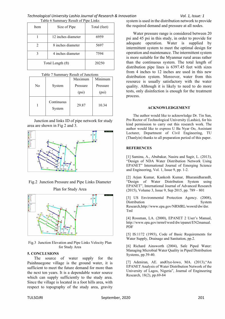
Technological University Lashio Journal of Research & Innovation Vol. 1, Issue: 1
TULSOJRI September, 2020 201
Table 6 Summary Result of Pipe Links
Item Size of Pipe Total (feet)
1 12 inches diameter 6959
2 8 inches diameter 5697
3 4 inches diameter 7594
Total Length (ft) 20250
Table 7 Summary Result of Junctions
No System
Maximum
Pressure
(psi)
Minimum
Pressure
(psi)
1 Continuous
System 29.87 10.34
Junction and links ID of pipe network for study area are shown in Fig 2 and 3.
Fig.2 Junction Pressure and Pipe Links Diameter
Plan for Study Area
Fig.3 Junction Elevation and Pipe Links Velocity Plan for Study Area
5. CONCLUSIONS
The source of water supply for the Painhnaegone village is the ground water, it is sufficient to meet the future demand for more than the next ten years. It is a dependable water source which can supply sufficiently to the study area. Since the village is located in a foot hills area, with respect to topography of the study area, gravity
system is used in the distribution network to provide the required demand and pressure at all nodes.
Water pressure range is considered between 20 psi and 45 psi in this study, in order to provide for adequate operation. Water is supplied by intermittent system to meet the optimal design for operation and maintenance. The intermittent system is more suitable for the Myanmar rural areas rather than the continuous system. The total length of distribution pipe lines is 6397.45 feet with sizes from 4 inches to 12 inches are used in this new distribution system. Moreover, water from this resource is usually satisfactory with the water quality. Although it is likely to need to do more tests, only disinfection is enough for the treatment process.
ACKNOWLEDGEMENT
The author would like to acknowledge Dr. Tin San, Pro Rector of Technological University (Lashio), for his kind permission to carry out this research work. The author would like to express U Ba Nyar Oo, Assistant Lecturer, Department of Civil Engineering, TU
(Thanlyin) thanks to all preparation period of this paper.
REFERENCES
[1] Saminu, A., Abubakar, Nasiru and Sagir, L. (2013), “Design of NDA Water Distribution Network Using EPANET” International Journal of Emerging Science and Engineering, Vol. 1, Issue 9, pp. 1-2.
[2] Arjun Kumar, Kankesh Kumar, BharanidharanB, “Design of Water Distribution System using EPANET”, International Journal of Advanced Research (2015), Volume 3, Issue 9, Sep 2015, pp. 789 – 801
[3] US Environmental Protection Agency. (2008), Distribution System Research,http://www.epa.gov/NRMRL/wswrd/dw/dsr. Tml
[4] Rossman, LA. (2000), EPANET 2 User’s Manual, http://www.epa.gov/nrmrl/wsrd/dw/epanet/EN2manual.PDF
[5] IS:1172 (1993), Code of Basic Requirements for Water Supply, Drainage and Sanitation, pp.2.
[6] Richard Ainsworth (2004), Safe Piped Water: Managing Microbial Water Quality in Piped Distribution Systems, pp.39-40.
[7] Adeniran, AE. andOye-lowo, MA. (2013),“An EPANET Analysis of Water Distribution Network of the University of Lagos, Nigeria”, Journal of Engineering Research, 18(2), pp.69-84

Technological University Lashio Journal of Research & Innovation Vol. 1, Issue: 1
TULSOJRI September, 2020 202
EXPERIMENTAL STUDY ON PRODUCTION OF BAMBOO FIBRE REINFORCED
CEMENT CEILING SHEET
Ei Mon Phyu(1), Win Mar Htet(2) (1)Pyay Technological University, Myanmar
(2)Pyay Technological University, Myanmar
Email: [email protected]
ABSTRACT: The ceiling sheet can be adapted
particularly for hot climates due to its high insulation
properties and therefore suitable to provide shelter
for livestock by using the locally available natural
fibre materials for its production. In this study,
natural fibre namely bamboo fibre as reinforcement
in cement and three different percentages of fly ash
as cement replacement material are used for
producing ceiling sheets. The ceiling sheet samples
(300mm x 300mm x 5mm) were manufactured by
using three different contents of fly ash (20%, 30%,
40%), water cement ratios of 0.4 and 0.5, 0.8% of
waste paper and 8% of bamboo fibre respectively.
For all samples, bending strength was carried out for
ages of 7 days and 28 days. From the test results, it
has been observed that the ceiling sheet at 30% fly ash
with water cement ratio 0.4 gives highest bending
strength and the lowest bending strength is at 40% fly
ash with water cement ratio 0.5. It can be studied that
the optimum percentage of fly ash is 30% for
replacement of cement and the bamboo fibre
reinforced cement ceiling sheet at 30% fly ash with
water cement ratio 0.4 is suitable for local use.
KEYWORDS: bamboo fibre, fly ash, bamboo fibre reinforced cement ceiling sheet, bending strength.
1. INTRODUCTION
Myanmar is a developing and tropical country.
Therefore, most of the people in rural area will affect the
thermal effect in hot season. Science and technology
make rapid advances and unforeseen changes about
construction in short period of time. The techniques to
produce low cost ceiling sheet are needed for rural areas
in our country. Among the many part of a house, ceiling
sheets are essential part of a house in the two major
climatic regions (warm humid and hot dry climates) in
order to insulate thermal effect. So, good quality and low
cost ceiling sheets should be manufactured by using
locally available materials. Natural fibres carry a major
portion of the tensile stress in the composite materials.
Plant fibres have a high strength and good insulation
properties (sound, electrical, and thermal). Bamboo
fibres can be got easily in our country and its strength is
enough to utilize in making ceiling sheets. To be
lightweight ceiling sheet, fly ash can be used in some
percentage of cement mix. Pozzolans may often be
cheaper than the cement and it can be used as a cement
replacement material. So, manufacturing cost can be
reduced by using fly ash (atrificial pozzolan) as a cement
replacement material. Since fly ash is waste material
from the coal industries, it makes advantages on
environment.
2. METHODOLOGY
Bamboo fibre reinforced cement ceiling sheet had
been produced by using materials of cement, class C fly
ash, Bamboo fibre, waste paper and water. In this study,
the mixing of materials is done by weighting. Three
ratios of fly ash contents of 20%, 30%, 40% were used
as a cement replacement material. The percentage of
fibre and waste paper were 8% and 0.8%. Two water-
cement ratios of 0.4 and 0.5 were used. The size of
specimen is 300 mm x 300mm x 5 mm. Physical
properties (Fineness, Soundness, Consistency, Setting
time and specific gravity) of cement and fly ash were
tested according to ASTM standard. Bending stress of
ceiling sheet sample was carried out to find the stress in
a material just before it yields in a flexure test.
3. MATERIALS USED
3.1 Cement
Ordinary Portland cement (Type I) was used in the
present experimental study. Double-Rhinoceros Cement
brand was used. Standard consistency is 30.1%
according to ASTM C187 [9]. The value of its specific
gravity was 2.9. The initial and final setting times were
found as 79.5 minutes and 165 minutes respectively
which were within ASTM Standard limits. Soundness of
this cement is good because its increase expansion of this
result test is 3 mm.
3.2. Fly Ash
Fly ash, also known as pulverized fuel ash in the
United Kingdom, is a coal combustion product. It is
composed of the particulates that are driven out of coal-
fired boilers together with the flue gases. In this study
Class C fly ash is used as cement replacement material.
According to ASTM 618, this fly ash is suitable as a
replacement material of cement. Test results of Class-C
fly ash are described in Table 1.
3.3 Bamboo fibres
Bamboo fibres are all cellulose fibres extracted from
natural bamboo. As natural cellulose fibre, it can be
100% biodegradable in soil by micro-organism and

Technological University Lashio Journal of Research & Innovation Vol. 1, Issue: 1
TULSOJRI September, 2020 203
sunlight. Its decomposition process doesn't cause any
pollution to environment. Bamboo used for fibre
preparation is usually 3-4 years old. The bamboo fibre
used in this study is shown in figure 1. The value of water
absorption for bamboo fibre is 46%. According to ACI,
this value must be between 40 and 50. So, the fibre is
suitable to use.
Table 1. Test Results of Class-C Fly Ash
Physical Properties Test Results Standard
ASTM limits
Fineness 21.68% <34
Standard
Consistency 29.25% 26 to 33
Initial Setting Time
(hr:min) 1:35 >45 min
Final Setting Time
(hr:min) 4:15 >10 hr
Specific Gravity 2.26 2.1 to 3.0
Fig 1 Bamboo fibre
3.4 Waste paper
This world also had facing the high amount of waste
product which including waste paper. Waste materials
can be reused directly or recycled to produce the same
or other products. This has benefits of not only reducing
the amount of waste material requiring disposal, but also
can produce usable production materials with significant
saving over the old ones. The waste paper can be reused
or used as recycled paper in the construction field. Paper
has been considered one of the most highly insulated
material and has regular pores and fibrous nature. So, the
paper pulp holds the moisture in these pores. Fibrous
nature gives very high energy absorbing ability and the
high compressive strength. In this manufacturing
process, paper bag of cement which is discarded after
using cement is used as waste paper. The average water
absorption of waste paper is 157%. Waste paper is
shown in figure 2.
Fig 2 Waste paper
4. MANUFACTURING PROCESS OF BAMBOO
FIBRE REINFORCED CEMENT CEILING
SHEET SPECIMEN
First of all, formwork (300 mm x 300 mm) which is
shown in figure 3 was prepared for ceiling sheet
fabrication. For quick and easy removal of ceiling sheets,
formworks were painted by red oxide and engine oil.
In the production of ceiling sheet, it is necessary to
make bamboo fibre before mixing. The bamboo is
collected from local sources and then it is properly
cleaned and cut into appropriate size of one inch. The
fibre should be clean and free from silt and dust.
In this study, the mixing of materials is done by
weighting. The mixing ingredients are cement, class C
fly ash, Bamboo fibre, waste paper and water. When dry
mix is completed, the right amount of water is added into
the mix on the impervious plate form. Water-cement
ratio of 0.4 and 0.5 is used to produce ceiling sheet. The
freshly mixed fibre reinforced cement mortar paste is
poured into formwork. The mortar paste is rammed
manually by using wooden rod for good compaction.
After about 24hr, the ceiling sheets can be removed from
the formwork. Finally, these ceiling sheets are emerged
into the water tank for curing. Ceiling sheet samples is
shown in figure 4. After curing, ceiling sheets reinforced
with bamboo fiber ware tested by bending tester machine
and the ceiling sheets gained acceptable strength are
ready to use.
Fig 3 Formwork

Technological University Lashio Journal of Research & Innovation Vol. 1, Issue: 1
TULSOJRI September, 2020 204
Fig 4 Ceiling Sheet Samples
5. BENDING STRENGTH TEST AND RESULTS
5.1 Bending Strength Test
The purpose of this research is to study the bending
strength of bamboo fibre reinforced cement ceiling sheet
with different fly ash. Bending strength is a material
property. It is defined as the stress in a material just
before it yields in a flexure test. The bending strength of
ceiling sheet is calculated by the following equation.
Bending strength test machine is shown in figure 5.
(1)
Where, f = Bending strength, psi
P = Breaking load, kg
L = Clear span between the supports, mm
b = Width of test specimen, mm
e = Actual average thickness of test specimen,
mm
Fig 5 Bending strength test machine
5.2. Results
The size of ceiling sheet sample is 300 mm x 300 mm x 5mm. The bending strength of ceiling sheet is carried out for 7 day and 28 day under testing machine. By studying the test results, it can be found that bending strength decreases as water cement ratio increases for each percentage of fly ash at ages of 7 days and 28 days. From the test results of 28 day, the specimen of 30 % fly
ash with water cement ratio 0.4 gives largest bending strength of 886.3 psi in all ratios of fly ash and that of 40% fly ash with water cement ratio 0.5 produces smallest bending strength of 777.7 psi. Bending strength test results for 7 day and 28 day are shown in Table 2, 3, 4 and 5. Average bending strengths of ceiling sheet samples for different content of fly ash after 7 and 28 days curing are also described in figure 6 and 7 respectively.
Table 2. Test Results of Bending Strength of Sample
for Water Cement Ratio 0.4 (7 day)
w/c Fly ash (%)
Sample
No
Bending Strength
(psi)
0.40
20%
1 556.2
2 560.8
3 548.3
Average 555.1
30%
1 660.8
2 652.6
3 655.2
Average 656.2
40%
1 515.4
2 528.6
3 523.7
Average 522.6
Table 3. Test Results of Bending Strength of Sample
for Water Cement Ratio 0.5 (7 day)
w/c Fly ash (%)
Sample
No
Bending Strength
(psi)
0.50
20%
1 518.46
2 511.2
3 516.8
Average 515.5
30%
1 572.9
2 575.6
3 580.3
Average 576.3
40%
1 463.1
2 469.9
3 476.8
Average 469.9

Technological University Lashio Journal of Research & Innovation Vol. 1, Issue: 1
TULSOJRI September, 2020 205
Table 4. Test Results of Bending Strength of Sample
for Water Cement Ratio 0.4 (28 day)
w/c Fly ash (%)
Sample
No
Bending Strength
(psi)
0.40
20%
1 840.9
2 846.9
3 848.5
Average 845.4
30%
1 886.9
2 885.2
3 886.9
Average 886.3
40%
1 810.9
2 808.6
3 809.6
Average 809.7
Table 5. Test Results of Bending Strength of Sample
for Water Cement Ratio 0.5 (28 day)
w/c Fly ash (%)
Sample
No
Bending Strength
(psi)
0.50
20%
1 833.6
2 830.2
3 829.9
Average 831.2
30%
1 866.8
2 867.2
3 868.9
Average 867.6
40%
1 778.4
2 774.9
3 779.8
Average 777.7
Fig 6 Average bending strengths of ceiling sheet samples
for different content of fly ash after 7 days
Fig 7 Average bending strengths of ceiling sheet samples
for different content of fly ash after 28 days
6. CONCLUSIONS
The bamboo fibre is available significant quantities
as a natural fibre and also fly ash is easily available and
economical among so many kinds of cementitious
materials in Myanmar. That is why it should be
considered to use bamboo fibre and fly ash for
reinforcement and replacement of cement in producing
ceiling sheet. Moreover, according to experimental result
of 28 days curing, the highest bending strength of
bamboo fibre reinforced cement ceiling sheet is at water
cement ratio 0.4 and 30 % replacement of fly ash with
the value of 886.3 psi and the lowest bending strength is
at water cement ratio 0.5 and 40% replacement of fly ash
with the value of 777.7 psi. It can be concluded that the
optimum percentage of fly ash is 30% for replacement of
cement and so the bamboo fibre reinforced cement
ceiling sheet has enough strength for local use.
ACKNOWLEDGEMENT
First and foremost, the author thanks to Professor Dr. Nyunt Soe, Rector of Pyay Technological University, for his invaluable permission. The author would like to express heart-felt gratitude to Dr. Mya San Wai, Professor and Head of Civil Engineering Department of PTU, for her encouragement and enthusiastic instruction. Special Thank to Dr. Yin Min Han, Professor and Head of Civil Engineering Department of Technological
0
100
200
300
400
500
600
700
20% 30% 40%
Ben
din
g S
tren
gth
(psi
)
Fly Ash (%)
W/C 0.4
W/C 0.5
700
750
800
850
900
20% 30% 40%Ben
din
g S
tren
gth
(psi
)Fly ash (%)
W/C 0.4
W/C 0.5
Technological University Lashio Journal of Research & Innovation Vol. 1, Issue: 1
TULSOJRI September, 2020 206
University (Toungoo) for her support, guidance and suggestions. The author would like to express her gratefulness to Daw Win Mar Htet, Lecturer, Civil Engineering Department of Pyay Technological University, for her sharing ideas and knowledge.
REFERENCES
[1] Ataguba, Clement Oguche, ‘‘Properties of Ceiling Board produced from A composite of Waste Paper
and Rice Husk’’, International Journal of Advances in Science Engineering and Technology, (Feb 2016)
[2] Ma War War Aung, ‘‘Study on Natural Fibre
Reinforced Roofing Sheet Using Locally Available
Materials’’, 2009
[3] Khairul Nizar Ismail, Kamarudin Hussin, Mohod
Sobri Idris,‘‘ Physical, Chemical and Mineralogical Properties of Fly Ash’’, Journal of Nuclear and Related TechnologyVol-4, (2007)
[4] Meyers-Levy, Joan, Zhu, Rui (Juliet), ‘‘The Influence of Ceiling Height: The Effect of Priming
on the Type of Processing That People Use’’, Journal of Consumer Research, (August 2007)
[5] Naw Myat Su Mon Htun, ‘‘A Study on the Application of Fly Ash as a Cement Replacement
Material with Super Plactizer for High Strength
Concrete’’, May 2005
[6] James I. Daniel Chairman, Vellore S. Gopalaratnam
Secretary, Melvyn A. Galinat Membership
Secretary, ‘‘Report on Fibre Reinforced Concrete’’, ACI 544.1R-96, 2002
[7] [90 Fai] Faisal Fouad Wafa, ‘‘ Properties and Application of Fibre Reinforced Concrete’’, January 1990M. King, B. Zhu, and S. Tang, “Optimal path planning,” Mobile Robots, vol. 8, no. 2, pp. 520-531,
March 2001.
[8] H. Simpson, Dumb Robots, 3rd ed., Springfield:
UOS Press, 2004, pp.6-9.
[9] American Standard Test Method for Normal
Consistency of Hydraulic ASTM C187-98
[10] American Standard Test Method for Time of
Setting of Hydraulic Cement by Vicat Needle
ASTM C191-04

Technological University Lashio Journal of Research & Innovation Vol. 1, Issue: 1
TULSOJRI September, 2020 207
Structural Behaviors Comparisons of RC Buildings with Two Different Flat Slab Types
Khine Zar Aung#1, Aung Min Tun#2
# Department of Civil Engineering, West Yangon Technological University Yangon, Republic of the Union of Myanmar
[email protected] [email protected]
ABSTRACT: There are many different systems
constructing reinforced concrete structure. Among them,
the flat slab system is the most popular in reinforcement
concrete structure for reduction the height of building.
Therefore, it is necessary to know the structural
behaviours of it. There are two types of flat slab systems:
one without drop panels and one with drop panels. The
objective of this journal is to compare between the
analysis results of the two buildings with above two
systems. This study deals with structural behaviours of
six-storeyed reinforced concrete building which is 45
feet wide, 60 feet long and 76 feet high. The proposed
buildings are situated in seismic zone 2B. Structural
Engineering Software (ETABS 2016, Version 16.2.0) is
used for analysis and design of the buildings. The
behaviours of the buildings have been investigated using
static analysis. According to MNBC 2016, all gravity
loads and lateral loads have to be applied. Soil profile
type is considered as (SD) stiff soil profile. Wind force
is exposure type B and basic wind velocity is 100 mph.
Finally, the results obtained are compared to investigate
the effects on structural behaviours of the building when
there is a difference in the type of flat slab used for the
building.
KEYWORDS: flat slab systems, structural behaviors.
1. INTRODUCTION
Nowadays, the high-rise reinforced concrete
buildings are widely used in Myanmar according to
political, social and economic demands and the potential
of its popularity will be greater in future. However, there
are encounter the height restriction laws in the location
of the proposed building. In this situation, flat slab
structures become a solution to the problem between the
height restriction law and the demand building height.
The use of flat slab provides many advantages over
conventional slab. The benefits of using flat slab
construction are becoming increasingly recognized. Flat
slabs without drops (thickened areas of slab around the
columns to resist punching shear) can be built faster
because formwork is simplified and minimized. Flat slab
construction places no restrictions on the positioning of
horizontal services and partitions, and can minimize
floor-to-floor heights when there is no requirement for a
deep false ceiling. This can have knock-on benefits in
terms of lower building height, reduced cladding costs
and prefabricated service. Flat slab construction offers
considerable flexibility to the occupier who can easily
alter internal layouts to accommodate changes in the use
of the structure. Lower storey height will reduce building
weight due to lower partitions and cladding to facade.
2. MODELLING OF REINFORCED CONCRETE
STRUCTURE WITH AND WITHOUT DROP
PANELS
The preparations for analysis and design
requirements and presentations of the analysis and
design results of the proposed buildings are considered.
The proposed reinforced concrete structure is 60 feet in
length, 45 feet in width and 76 feet in height.
Fig 1. Typical Floor Plan of Proposed Buildings
The site location and structural system are chosen
before modeling for the design of proposed buildings.
Then, there are considered material properties of the
structures, determination of load combinations, and
selection of codes according to MNBC 2016 and ACI
318-14 for the analysis and design of proposed buildings.
ETABS 2016 (Version 16.2.0) is used to analysis and

Technological University Lashio Journal of Research & Innovation Vol. 1, Issue: 1
TULSOJRI September, 2020 208
design the structures in this study. In the analysis and
design of structures, the purpose of analysis is to
determine the stress and displacements in the various
member of a structure. Structural stability check is made
whether it is satisfactory or not. Then, the reinforcements
of structural members are calculated.
2.1 Material properties
Analysis property data,
Weight per unit volume of concrete : 150 pcf
Modulus of elasticity : 4.0305 x 10⁶ psi
Poisson’s ratio : 0.2
Coefficient of thermal expansion :5.5 x 10⁻⁶ in/in per ˚F
Reinforcing yield strength (fy) : 60000 psi
Concrete cylinder strength (fc') : 5000 psi
Shear reinforcing yield strength (fys) : 60000 psi
2.2 Loading Data for gravity load
Data for gravity load which are used in structural
analysis are as follows:
Superimposed dead load = 20 psf
(Ceiling is considered as superimposed dead loads)
Design data for live loads which are used in the
analysis are as follows.
Live load on stair = 100 psf
Live load on roof = 20 psf
Live load all other areas = 40 psf
2.3 Data for wind load
Data for wind load which are used in structural
analysis are as follow:
Site Location - Yangon
Exposure type - B
Effective height for wind load - 76 feet
Method - Analytical Procedure
Basic wind Speed - 100 mph
Gust factor - 0.85
Directionality factor - 0.85
Topographical factor - 1.0
Wind important factor - 1.0
2.4 Data for earthquake load
Data for earthquake load which are used in
structural analysis are as follow:
Seismic zone = 2B (Yangon)
0.2 sec spectral acceleration = 0.77
1 sec spectral acceleration = 0.31
Soil profile type = SD
Design moment frame type = IMRF
Response modification factor (R) = 5
System over-strength factor (Ω) = 3
Deflection amplification factor (Cd) = 4.5
Long-period transition (TL) = 6 sec
Seismic importance factor (I) = 1.00
Approximate period parameters for concrete
moment resisting frames are:
Ct = 0.016
x = 0.9
2.5 Load Combinations
Design codes applied are ACI 318-14 and MNBC-
2016.There are 23 numbers of load combinations in
MNBC-2016.
3. DESIGN CONSIDERATIONS
In this study, the structural members are analyzed
and design according to ACI 318-14. The design sections
of structural member are C24x24, C22x22 and C20x20
in columns and B 14x18 is used as perimeter beam. Both
building have the same layout plans of beams and
columns, but with different reinforcement, especially in
beams. In slab thickness, 10 inches is used as flat slab in
RC building without drop panel and 8 inches is used the
one with drop panel. The size of drop panel is 5 feet.x 4
feet x 10 inches.
Fig 2. Layout Plan of Drop Panels
After the sizes of members are satisfied under
MNBC-2016 load combinations, the buildings with and
without drop panels are also checked in stability such as
base shear, overturning moment, sliding, drift ratio, P-
Del effect, torsional irregularity and soft storey effects.

Technological University Lashio Journal of Research & Innovation Vol. 1, Issue: 1
TULSOJRI September, 2020 209
Punching shear check is required in flat slab in both
systems.
Table1. Slab Schedule for Building With Drop Panels
Storey
Thickness Lay
er
Reinforcement Distrib
ution Slab Drop
Panel Shorter Longer
RF and
SR 8 in 10 in
Top 14mm@12
in c/c
14mm@12
in c/c -
Bott
om
14mm@
12in c/c
14mm@12in
c/c -
1F to
5F 8 in 10 in
Top 14mm @ 8
in c/c
14mm@ 8 in
c/c -
Bott
om
14mm @ 8
in c/c
14mm@ 8 in
c/c -
Stair 6 in
Top - 12mm@6 in
c/c
10mm
@10in
c/c
Bott
om -
12mm@6 in
c/c
10mm
@10in
c/c
Table 2.Slab Schedule for Building Without Drop panel
Storey Thick
ness Layer
Reinforcement Distribution
Shorter Longer
RF
and
SR
10 in
Top 14mm@
10 in c/c
14mm@
10in c/c -
Bottom 14mm@
10in c/c
14mm@
10in c/c -
1F to
5F 10 in
Top 14mm
@ 8 in c/c
14mm
@ 8 in c/c -
Bottom 14mm@ 8
in c/c
14mm@
8in c/c -
Stair 6 in
Top - 12mm
@6 in c/c
10mm
@10in c/c
Bottom - 12mm
@6 in c/c
10mm
@10in c/c
4. ANALYSIS RESULTS AND DISCUSSIONS
The gravity loading due to dead load and live load
and lateral loading due to wind or earthquake are the
major factors that cause different displacements and
forces in reinforced concrete structure with and without
drop panels. There are seven critical behaviours on this
structure. In this section, comparisons between two
buildings based on storey drifts, P-∆, torsional irregularity, overturning, sliding, punching shear and soft
storey are presented.
4.1 Comparison on Storey Drift
According to the fig. 3 and fig.4 for the two
buildings, the drifts of the building without drop panels
are larger in both directions than the building with drop
panels. The drift of the former is 15% greater than that of
the latter at stair roof in X-direction .
Fig 3. Comparison on Storey Drift in X-direction
Fig.3. Comparison on Storey Drift in X-direction
Fig. Error! No text of specified style in
document.. Comparison on Storey Drift in Y-direction
A. Comparison on P-∆ Effect
Fig 4. Comparison on Storey Drift in Y-direction
4.2 Comparison on P-∆ Effect
Fig 5. Comparison of P-∆ in X-direction
Fig 6. Comparison of P-∆ in Y-direction
According to the fig. 5 and fig. 6 for the two
buildings, the stability coefficient values of the building
without drop panels are larger in both directions than the
building with drop panels since the former has higher
secondary moment (larger weight and higher drift) than
the latter. The coefficient value of the former is 17%
greater than that of the latter at roof in X-direction.
0.000
5.000
S R R F 5 F 4 F 3 F 2 F 1 F G F
DR
IFT
(IN
)
STOREY
Without Drop Panels
With Drop Panels
Drift Limit
0.000
5.000
S R R F 5 F 4 F 3 F 2 F 1 F G F
DR
IFT
(IN
)
STOREY
Without Drop Panels
With Drop Panels
Drift Limit
0.000
0.050
0.100
0.150
S R R F 5 F 4 F 3 F 2 F 1 F G F
ST
AB
ILIT
Y
CO
EF
FIC
IEN
T
STOREY
Without Drop Panels
With Drop Panels
Limit
0.000
0.050
0.100
0.150
S R R F 5 F 4 F 3 F 2 F 1 F G F
ST
AB
ILIT
Y
CO
EF
FIC
IEN
T
STOREY
Without Drop Panels
With Drop Panels
Limit

Technological University Lashio Journal of Research & Innovation Vol. 1, Issue: 1
TULSOJRI September, 2020 210
4.3 Comparison on Torsional Irregularity
Fig 7. Comparison of Torsional Irregularity in X-
direction
Fig 8. Comparison of Torsional Irregularity in Y-
direction
As for the two buildings, the building with drop
panels is reasonably stronger in resistance to torsional
irregularity for both directions than the building without
drop panels, relating with variation in cross-section and
weight of slab according to fig. 7 and 8.
4.4 Comparison on Overturning and Sliding
Fig. 9. Comparison on Overturning
Fig 10. Comparison on Sliding
In Fig. 9 and 10, the building without drop panels
has slightly higher resistance to overturning and sliding
in both directions than the building with drop panels.
This is because the former has larger weight due to
uniformly thicker slabs throughout the spans than the
latter, slabs of which only have large thickness in the
areas of drop panels, comprising at the difference in slab
weight of 324 kips. The overturning and sliding S.F
values of the former are 9% and 2% respectively greater
than that of the latter as overall building in X-direction.
4.4 Comparison on Punching Shear
According to fig.11 the building without drop panels
have smaller resistance to punching shear failure than the
buildings with drop panels since drop panels provide
additional shear strength around the column. The
punching shear ratio of the former is 27% greater than
that of the latter at stair roof.
Fig 11. Comparison on Punching Shear
4.5 Comparison on Soft Storey
Figure 4.12 and figure 4.13 illustrate that both
buildings have no soft storey effects.
As for the directions, both buildings have higher
storey stiffness in Y-direction than in X-direction.
As for the two buildings, the building without drop
panels has moderately weaker storey stiffness than the
building with drop panels. In 70% storey stiffness
limitation, the stiffness value of the former is 4% smaller
than that of the latter at fifth floor in X-direction.
0.000
1.000
2.000
3.000
4.000
5.000
X Y
SA
FE
TY
FA
CT
OR
DIRECTION
Without Drop Panels
With Drop Panels
Minimum S.F
1.400
1.600
1.800
X Y
SA
FE
TY
FA
CT
OR
DIRECTION
Without Drop Panels
With Drop Panels
Minimum S.F
0.000
0.500
1.000
1.500
StairRF
RF 5F 4F 3F 2F 1F
MA
X P
UN
CH
ING
SH
EA
R
RA
TIO
STOREY
Without Drop Panels
With Drop Panels
Limit
0.900
1.000
1.100
1.200
1.300
S R R F 5 F 4 F 3 F 2 F 1 F G FMA
X-T
O-A
VG
DR
FIT
RA
TIO
STOREY
Without Drop Panels
With Drop Panels
Limit
0.900
1.000
1.100
1.200
1.300
S R R F 5 F 4 F 3 F 2 F 1 F G FMA
X-T
O-A
VG
DR
FIT
RA
TIO
STOREY
Without Drop Panels
With Drop Panels
Limit

Technological University Lashio Journal of Research & Innovation Vol. 1, Issue: 1
TULSOJRI September, 2020 211
Fig 12. Comparison on Soft Storey in X Direction
Fig 13. Comparison on Soft Storey in Y Direction
5. CONCLUSION
From the above study, it can be concluded as the
following.
(1) The drift ratio in third floor is the maximum in
both X direction and Y direction. The drifts without drop
panels are larger in both directions than that with drop
panels. Therefore, the structural behavior of the building
with drop panel is stiffer than that of without drop panel
according to drift.
(2) According to the stability coefficient values of
the building, the higher the building, the more increase
the stability coefficient in both with and without drop
panels. The stability coefficients without drop panel are
larger in both directions than that of the building with
drop panels, apparently being 17% greater at roof in X-
direction.
(3) The Torsional irregularity does not occur in both
systems and this value is the maximum in roof
reasonably. According to the building geometry,
maximum-to-average drift ratios in X direction is smaller
than that in Y direction. The building without drop panels
is reasonably stronger in resistance to torsional
irregularity for both directions than the building with
drop panels, with the slightly smaller maximum-to-
average drift ratios, obviously being 9% smaller at roof
in X-direction.
(4) In the case of overturning moment, that in X
direction is smaller than that in Y direction because of
the geometry. The building without drop panels have
slightly higher resistance to overturning in both
directions than the building with drop panels, with the
slightly larger S.F values, obviously being 9% greater for
overturning in X-direction. The case of sliding is the
same manner of overturning moment.
(5) The buildings with both systems do not occur
soft storey effect in 70% stiffness case and 80% stiffness
case. The stiffness of building without drop panels is
nearly equal to that with drop panels in both directions.
ACKNOWLEDGEMENTS
The authors are extremely grateful to the teachers
from Department of Civil Engineering in West Yangon
Technological University, for their guidance, advice and
encourages for completing this paper.
REFERENCES
[1] ACI Committee 318. 2014. 318-14: Building Code Requirement for Structural Concrete and Commentary. U.S.A: American Concrete Institute.
[2] Bijan O Aalami. 2008. Deflection of Concrete Floor Systems for Serviceability. India: ADAPT
International Pvt. Ltd.
[3] Harshal Deshpande, Radhika Joshi, Prashant
Bangar. 2014. “Design Considerations for Reinforced Concrete Flat Slab Floor System”. International Journal of Scientific and Engineering Research, vol.5, no.12 (December)
[4] International Conference of Building Officials.
1997. “Structural Engineering Design Provisions”. Uniform Building Code, vol.2, U.S.A.
[5] Lindeburg and McMullin. 2008: Seismic Design of Building Structure. 8th ed. U.S.A: Professional
Publication. Inc.
[6] Myanmar Engineering Council. 2016. “Structural Design”. Myanmar National Building Code 2016,
vol.3, Yangon.
0.000
10.000
20.000
30.000
StairRF
RF5F4F3F2F1FGF
ST
IFF
NE
SS
(H
UN
DR
ED
S O
F K
IP P
ER
IN
)
STOREY70% Stiffness of Storey AboveWithout Drop Panels70% Stiffness of Storey Above WithDrop Panels80% Average Stiffness of ThreeStoreys Above Without Drop Panels80% Average Stiffness of ThreeStoreys Above With Drop PanelsStorey Stiffness Without Drop Panels
Storey Stiffness With Drop Panels
0.000
20.000
40.000
StairRF
RF5F4F3F2F1FGF
ST
IFF
NE
SS
(H
UN
DR
ED
S O
F K
IP P
ER
IN
)
STOREY70% Stiffness of Storey Above WithoutDrop Panels70% Stiffness of Storey Above WithDrop Panels80% Average Stiffness of Three StoreysAbove Without Drop Panels80% Average Stiffness of Three StoreysAbove With Drop PanelsStorey Stiffness Without Drop Panels
Storey Stiffness With Drop Panels


