RIMS Kokyuroku BessatsuBx (201x), 000–000
Commensurability of hyperbolic Coxeter groups:
theory and computation
By
Rafael Guglielmetti∗, Matthieu Jacquemet∗∗
and Ruth Kellerhals∗∗∗
Abstract
For hyperbolic Coxeter groups of finite covolume we review and present new theoretical
and computational aspects of wide commensurability. We discuss separately the arithmetic
and the non-arithmetic cases. Some worked examples are added as well as a panoramic view
to hyperbolic Coxeter groups and their classification.
§ 1. Introduction
Consider two discrete groups Γ1,Γ2 ⊂ IsomHn , n ≥ 3 , with fundamental polyhe-
dra P1, P2 of finite volume, respectively. The groups Γ1,Γ2 are said to be commensurable
(in the wide sense) if the intersection of Γ1 with some conjugate Γ′2 of Γ2 in IsomHn
has finite index in both, Γ1 and Γ′2. In this case, the orbifolds Hn/Γ1 and Hn/Γ2 are
covered, with finite sheets and up to isometry, by a common hyperbolic n-manifold.
Or, in other words, there is a hyperbolic polyhedron P ⊂ Hn which is simultaneously
glued by finitely many copies of P1 and by finitely many copies of P2. In particular, the
quotient of the volumes of P1 and P2 is a rational number.
Consider a Coxeter group Γ ⊂ IsomHn of rank N , that is, Γ is a discrete group
generated by finitely many reflections si , 1 ≤ i ≤ N , in hyperplanes of Hn. A funda-
mental polyhedron P for Γ is a Coxeter polyhedron, that is, a convex polyhedron with
Received April 20, 201x. Revised September 11, 201x.2010 Mathematics Subject Classification(s):Key Words: Hyperbolic Coxeter group, discrete reflection group, arithmetic group, commensurator,amalgamated product, crystallographic group
∗University of Fribourg, Fribourg, Switzerland.e-mail: [email protected]
∗∗Vanderbilt University, Nashville, USA.e-mail: [email protected]
∗∗∗University of Fribourg, Fribourg, Switzerland.e-mail: [email protected]
c© 201x Research Institute for Mathematical Sciences, Kyoto University. All rights reserved.
2 Guglielmetti, Jacquemet, Kellerhals
(non-zero) dihedral angles of the form π/m for integers m ≥ 2. Such groups are charac-
terised by a particularly nice presentation (see (2.2)) and provide – for small N ≥ n+ 1
– an important class of hyperbolic n-orbifolds and n-manifolds of small volumes.
In [30], the hyperbolic Coxeter n-simplex groups (of rank N = n + 1) of finite
covolume were classified up to commensurability. They exist for n ≤ 9, only. In [24],
the authors resolved the commensurability problem for the considerably larger fam-
ily of hyperbolic Coxeter pyramid groups, existing up to n = 17. They are of rank
N = n + 2 and have fundamental polyhedra which are combinatorially pyramids with
apex neighborhood given by a product of two simplices of positive dimensions; they
were discovered by Tumarkin [52], [54]. Among the 200 examples in this class are arith-
metic and non-arithmetic groups. Furthermore, modulo finite index, all these groups
have fundamental polyhedra which are (polarly and simply) truncated simplices, and
at times they arise as amalgamated free products. This indicates why several different
algebraic and geometric methods had to be developped in [24] in order to achieve the
commensurability classification.
In this work we present various of these general methods allowing us to decide
about commensurability of hyperbolic Coxeter groups. We illustrate the theory in
detail by providing several typical and also new examples. In Section 2, we furnish the
necessary background about hyperbolic Coxeter groups, including volume identities in
three dimensions, and add a panoramic view to hyperbolic Coxeter polyhedra known so
far. Since arithmeticity is a commensurability invariant, we discuss this aspect in a quite
complete and self-contained way (see Section 4). For non-arithmetic Coxeter pyramid
groups Γ ⊂ IsomHn with non-compact quotient space Hn/Γ, the commensurability
classification is based on geometric results exploiting the presence and the nature of
Bieberbach groups and their full rank translational lattices in a thorough way. We
summarise the corresponding results, only, and refer to [24, Section 4.1] for technical
details and proofs. In the case of certain non-arithmetic groups in IsomH3 which are
seemingly incommensurable, we manage to provide a rigorous proof by means of their
commensurator group (see Section 3.1) and an adequate covolume comparison (see
Section 5.4).
At the end of the work are appended the list of the 23 non-compact Coxeter tetra-
hedra and their volumes, the list of Tumarkin’s Coxeter pyramids as well as the classi-
fication tables of all arithmetic and non-arithmetic hyperbolic Coxeter pyramid groups,
respectively.
Acknowledgements
This work is based on the authors’ article [24], Section 5 of the PhD thesis [27] of
Matthieu Jacquemet, Chapter 4 of the PhD thesis [23] of Rafael Guglielmetti, and the
three talks held by Rafael Guglielmetti and Ruth Kellerhals on the occasion of the RIMS
Commensurability of hyperbolic Coxeter groups: theory and computation 3
Symposium on Geometry and Analysis of Discrete Groups and Hyperbolic Spaces, June
22–26, 2015. Rafael Guglielmetti and Ruth Kellerhals would like to thank Professor
Michihiko Fujii and the Research Institute for Mathematical Sciences (RIMS), Kyoto
University, for the invitation, the generous support and the hospitality.
The first author was fully and the third author was partially supported by Schweiz-
erischer Nationalfonds 200020–144438 and 200020–156104. The second author is sup-
ported by Schweizerischer Nationalfonds P2FRP2–161727.
§ 2. Preliminaries
§ 2.1. Hyperbolic Coxeter groups and Coxeter polyhedra
Denote by Xn either the Euclidean space En, the sphere Sn, or the hyperbolic space
Hn, and let IsomXn be its isometry group. As for the sphere Sn ⊂ En+1, embed Hn in
a quadratic space Yn+1. More concretely, we view Hn in the Lorentz-Minkowski space
En,1 = (Rn+1, 〈x, y n,1 =∑ni=1 xiyi − xn+1yn+1) of signature (n, 1) so that
Hn = x ∈ En,1 | 〈x, x n,1 = −1, xn+1 > 0
(see [59], for example). The group IsomHn is then isomorphic to the group PO(n, 1) of
positive Lorentz-matrices. In the Euclidean case, we take the affine point of view and
write Yn+1 = En × 0.A geometric Coxeter group is a discrete subgroup Γ ⊂ IsomXn generated by finitely
many reflections in hyperplanes of Xn. The cardinality N of the set of generators is
called the rank of the group Γ.
Let si be a generator of the geometric Coxeter group Γ acting on Xn as the reflection
with respect to the hyperplane Hi (1 ≤ i ≤ N). Associate to Hi a normal unit vector
ei ∈ Yn+1 such that
Hi = x ∈ Xn | 〈x, ei Yn+1 = 0 ,and which bounds the closed half-space
H−i = x ∈ Xn | 〈x, ei Yn+1 ≤ 0 .
A convex (closed) fundamental domain P = P (Γ) ⊂ Xn of Γ can be chosen to be given
by the polyhedron
(2.1) P =
N⋂i=1
H−i .
By Vinberg’s work [59], the combinatorial, metrical and arithmetical properties of P
and Γ, respectively, can be read off from the Gram matrix G(P ) of P formed by the
4 Guglielmetti, Jacquemet, Kellerhals
products 〈ei, ej Yn+1 ( 1 ≤ i, j ≤ N). In the hyperbolic case, the product 〈ei, ej n,1characterises the mutual position of the hyperplanes Hi, Hj as follows.
−〈ei, ej n,1 =
cos π
mijif Hi, Hj intersect at the angle π
mijin Hn,
1 if Hi, Hj meet at ∂Hn,cosh lij if Hi, Hj are at distance lij in Hn.
A fundamental domain P ⊂ Xn as in (2.1) for a geometric Coxeter group is a
Coxeter polyhedron, that is, a convex polyhedron in Xn all of whose dihedral angles are
submultiples of π. Conversely, each Coxeter polyhedron in Xn gives rise to a geometric
Coxeter group.
The geometric Coxeter group Γ has the presentation
(2.2) Γ = 〈 s1, . . . , sN | s2i , (sisj)
mij
for integers mij = mji ≥ 2 for i 6= j.
We restrict our attention to cocompact or cofinite geometric Coxeter groups, that is,
we assume that the associated Coxeter polyhedra are compact or of finite volume in Xn.
In particular, hyperbolic Coxeter polyhedra are bounded by at least n+ 1 hyperplanes,
appear as the convex hull of finitely many points in the extended hyperbolic space
Hn ∪ ∂Hn and are acute-angled (less than or equal to π2 ). An (ordinary) vertex p ∈ Hn
of P is given by a positive definite principal submatrix of rank n of the Gram matrix
G(P ) of P . Its vertex figure Pp is an (n− 1)-dimensional spherical Coxeter polyhedron
which is a product of k ≥ 1 pairwise orthogonal lower-dimensional spherical Coxeter
simplices. A vertex (at infinity) q ∈ ∂Hn of P is characterised by a positive semi-definite
principal submatrix of rank n − 1 of the Gram matrix G(P ). Its vertex figure Pq is a
compact (n− 1)-dimensional Euclidean Coxeter polyhedron which is a product of l ≥ 1
pairwise orthogonal lower-dimensional Euclidean Coxeter simplices. The polyhedron
Pq is a fundamental domain of the stabiliser Γq of q which is a crystallographic group
containing a finite index translational lattice of rank n− 1 by Bieberbach’s Theorem.
Many of these properties can be read off from the Coxeter graph Σ of P and Γ. To
each hyperplane Hi of P and to each generator si ∈ Γ corresponds a node νi of Σ. Two
nodes νi, νj are joined by an edge with label mij ≥ 3 if ](Hi, Hj) = π/mij (the label 3
is usually omitted). If Hi, Hj are orthogonal, their nodes are not connected. If Hi, Hj
meet at ∂Hn, their nodes are joined by an edge with label∞ (or by a bold edge); if they
are at distance lij > 0 in Hn, their nodes are joined by a dotted edge, often without
the label lij . We will also use the Coxeter symbol for a Coxeter group. For example,
[p, q, r] is associated to a linear Coxeter graph with 3 edges of consecutive labels p, q, r,
and the Coxeter symbol [(p, q, r)] describes a cyclic graph with labels p, q, r. Often, we
abbreviate further and write [p2] instead of [p, p], and so on. The Coxeter symbol [3i,j,k]
Commensurability of hyperbolic Coxeter groups: theory and computation 5
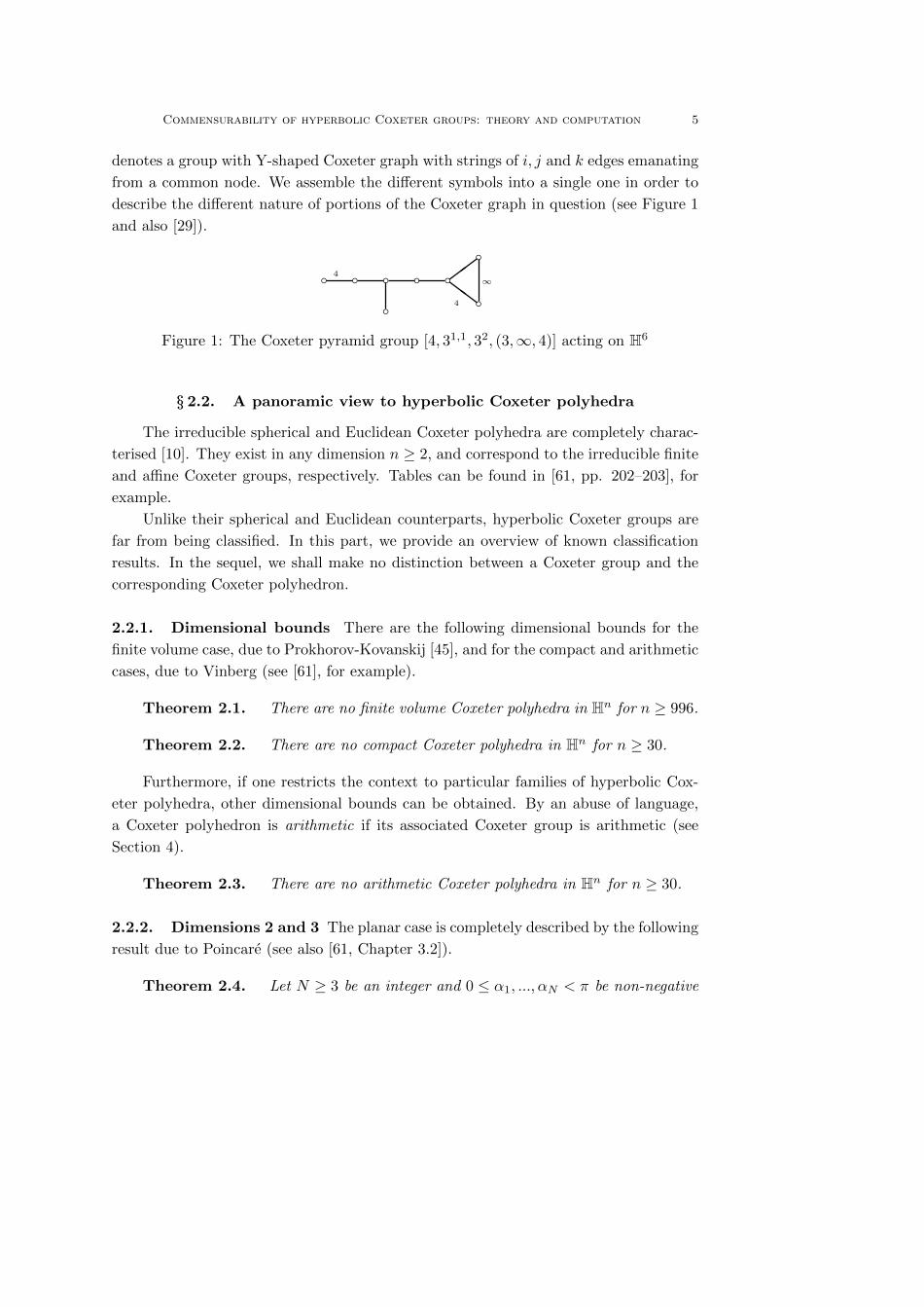
denotes a group with Y-shaped Coxeter graph with strings of i, j and k edges emanating
from a common node. We assemble the different symbols into a single one in order to
describe the different nature of portions of the Coxeter graph in question (see Figure 1
and also [29]).
b b bb b b bb
ZZ
4
4
∞
Figure 1: The Coxeter pyramid group [4, 31,1, 32, (3,∞, 4)] acting on H6
§ 2.2. A panoramic view to hyperbolic Coxeter polyhedra
The irreducible spherical and Euclidean Coxeter polyhedra are completely charac-
terised [10]. They exist in any dimension n ≥ 2, and correspond to the irreducible finite
and affine Coxeter groups, respectively. Tables can be found in [61, pp. 202–203], for
example.
Unlike their spherical and Euclidean counterparts, hyperbolic Coxeter groups are
far from being classified. In this part, we provide an overview of known classification
results. In the sequel, we shall make no distinction between a Coxeter group and the
corresponding Coxeter polyhedron.
2.2.1. Dimensional bounds There are the following dimensional bounds for the
finite volume case, due to Prokhorov-Kovanskij [45], and for the compact and arithmetic
cases, due to Vinberg (see [61], for example).
Theorem 2.1. There are no finite volume Coxeter polyhedra in Hn for n ≥ 996.
Theorem 2.2. There are no compact Coxeter polyhedra in Hn for n ≥ 30.
Furthermore, if one restricts the context to particular families of hyperbolic Cox-
eter polyhedra, other dimensional bounds can be obtained. By an abuse of language,
a Coxeter polyhedron is arithmetic if its associated Coxeter group is arithmetic (see
Section 4).
Theorem 2.3. There are no arithmetic Coxeter polyhedra in Hn for n ≥ 30.
2.2.2. Dimensions 2 and 3 The planar case is completely described by the following
result due to Poincare (see also [61, Chapter 3.2]).
Theorem 2.4. Let N ≥ 3 be an integer and 0 ≤ α1, ..., αN < π be non-negative
6 Guglielmetti, Jacquemet, Kellerhals
real numbers such that
(2.3) α1 + ...+ αN < (N − 2)π.
Then, there exists a hyperbolic N -gon P ⊂ H2 with angles α1, ..., αN . Conversely, if
0 ≤ α1, ..., αN < π are the angles of an N -gon P ⊂ H2, then they satisfy (2.3).
In particular, the set of hyperbolic Coxeter polygons with N sides can be identified
with the set of N -tuples given by
(p1, ..., pN ) | 2 ≤ pi ≤ ∞,∑Ni=1
1pi< N −2
over Z.
The situation in the 3-dimensional case becomes already more subtle. For compact
acute-angled polyhedra, that is, all dihedral angles are less than or equal to π2 , there is
the following result due to Andreev [3], which has been fully proved by Roeder [47, 48].
Theorem 2.5. Let P ⊂ H3 be a compact acute-angled polyhedron with N ≥ 5
facets and M ≥ 5 edges with corresponding dihedral angles α1, ..., αM . Then,
1. For all i = 1, ...,M , αi > 0.
2. If three edges ei, ej , ek meet at a vertex, then αi + αj + αk > π.
3. For any prismatic 3-circuit with intersecting edges ei, ej , ek, one has αi+αj +αk <
π.
4. For any prismatic 4-circuit with intersecting edges ei, ej , ek, el, one has αi + αj +
αk + αl < 2π.
5. For any quadrilateral facet F bounded successively by edges ei, ej , ek, el such that
eij , ejk, ekl, eli are the remaining edges of P based at the vertices of F (epq is based
at the intersection of ep and eq), then
αi + αk + αij + αjk + αkl + αli < 3π
and
αj + αl + αij + αjk + αkl + αli < 3π.
Furthermore, the converse holds, i.e. any abstract 3-polyhedron satisfying the conditions
above can be realised as a compact acute-angled hyperbolic 3-polyhedron, and is unique
up to isometry.
Andreev also extended his result to the non-compact case [4]. Let us mention that
the special case of ideal polyhedra, that is, polyhedra all of whose vertices lie on ∂Hn,
admits a simple formulation using the dual of a polyhedron: Recall that the dual of a
polyhedron P ⊂ H3 is the polyhedron P ∗ such that the set of vertices of P is in bijection
with the set of facets of P ∗, and vice-versa. Furthermore, for any edge e of P associated
to a dihedral angle α, the corresponding edge e∗ of P ∗ supports a dihedral angle α∗
given by α∗ = π − α. The result, due to Rivin [46] (see also [21]), reads as follows.
Commensurability of hyperbolic Coxeter groups: theory and computation 7
Theorem 2.6. Let P ⊂ H3 be an ideal polyhedron. Then, its dual P ∗ ⊂ H3
satisfies the following conditions.
1. For any dihedral angle α∗ of P ∗, one has 0 < α∗ < π.
2. If the edges e∗1, ..., e∗k with associated dihedral angles α∗1, ..., α
∗k form the boundary of
a facet of P ∗, thenk∑i=1
α∗i = 2π.
3. If the edges e∗1, ..., e∗k with associated dihedral angles α∗1, ..., α
∗k form a closed circuit
in P ∗ but do not bound a facet, then
k∑i=1
α∗i > 2π.
Moreover, any polyhedron P ∗ ⊂ H3 satisfying the above conditions (1)− (3) is the dual
of some ideal polyhedron P ⊂ H3, which is unique up to isometry.
2.2.3. Classifications in terms of the number of facets
Let P ⊂ Hn be a finite volume Coxeter polyhedron with N ≥ n+1 facets. Complete
classifications have been obtained for N = n + 1 and N = n + 2 only. For N = n + 1
and hyperbolic Coxeter simplices, the classification is due to Lanner in compact case
and to Koszul in the finite volume case.
Theorem 2.7 (N = n+ 1).
• Compact hyperbolic Coxeter simplices exist in dimensions n = 2, 3 and 4 only. For
n = 3, 4, there are finitely many of them.
• Finite-volume non-compact hyperbolic Coxeter simplices exist in dimensions n =
2, ..., 9 only. For 3 ≤ n ≤ 9, there are finitely many of them.
Tables can be found in [61, p. 203 and pp. 206–208], for example. For n = 3, the
non-compact Coxeter tetrahedra of finite volume are listed in Appendix Appendix A.
If N = n + 2, then P is either a prism, or a product of two simplices of positive
dimensions, or a pyramid over the product of two simplices of positive dimensions. The
respective classification is due to Kaplinskaja [32], Esselmann [14] and Tumarkin [54].
Theorem 2.8 (N = n+ 2).
• Compact, respectively finite-volume, Coxeter prisms in Hn exist only for n ≤ 5. For
4 ≤ n ≤ 5, there are finitely many of them.
8 Guglielmetti, Jacquemet, Kellerhals
• Compact Coxeter polyhedra with n+ 2 facets in Hn which are not prisms exist only
for n ≤ 4. For n = 4, there are exactly 7 of them.
• Finite-volume Coxeter polyhedra with n+ 2 facets in Hn which are not prisms exist
only for n ≤ 17. For 3 ≤ n ≤ 17, there are finitely many of them.
Tables can be found in [32, pp. 89–90], [61, p. 61], [14, p. 230] respectively
while the list [54] of Tumarkin’s Coxeter pyramids which are pyramids over a product
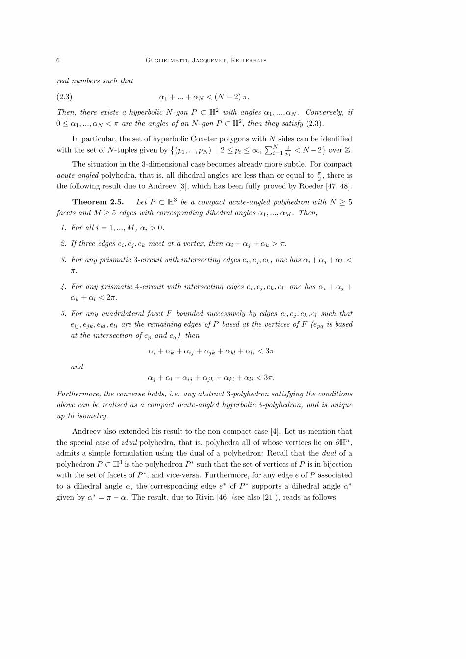
of two simplices of positive dimensions is attached in Appendix Appendix B. Notice
that among the non-compact Coxeter polyhedra with n + 2 facets in Hn, n ≥ 3, the
polyhedra of Tumarkin are the only ones apart from the Coxeter polyhedron P ⊂ H4
depicted in Figure 2 which is combinatorially a product of two triangles.
b bb bb b
@@@
@@@
4
4
4
4
Figure 2: The Coxeter polyhedron P ⊂ H4
In this work, the family of Tumarkin’s pyramids will be of special interest. Such
a pyramid is not compact since its apex, with a neighborhood being a cone over a
product of two Euclidean simplices, has to be a point at infinity. In the associated
Coxeter graph Σ, the node separating Σ into the two disjoint corresponding Euclidean
Coxeter subgraphs is encircled. Let us just mention a few particular features of the
family of Tumarkin’s Coxeter pyramid groups. It has 200 members, with examples up
to dimension n = 17, and comprises non-arithmetic groups up to dimension 10. There
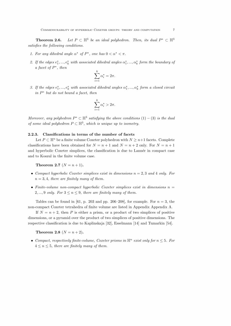
is a single but very distinguished group Γ∗ in dimension 17.
b b bb b b b b b ce b b b b b b bb bFigure 3: The graph of the Coxeter pyramid P∗ = [32,1, 312, 31,2] in H17
The group Γ∗ is closely related to the even unimodular group PSO(II17,1) in the
following way. Denote by P∗ the Coxeter polyhedron associated to Γ∗ whose Cox-
eter graph is given in Figure 3. By a result of Emery [12, Theorem 1], the orbifold
H17/PSO(II17,1) is the (unique up to isometry) hyperbolic n-space form of minimal
volume among all orientable arithmetic hyperbolic n-orbifolds for n ≥ 2. Its volume
can be identified with the one of P∗ and computed according to (see [12, Section 3])
vol17(P∗) = vol17(H17/PSO(II17,1)) =691 · 3617
238 · 310 · 54 · 72 · 11 · 13 · 17ζ(9) .
Commensurability of hyperbolic Coxeter groups: theory and computation 9
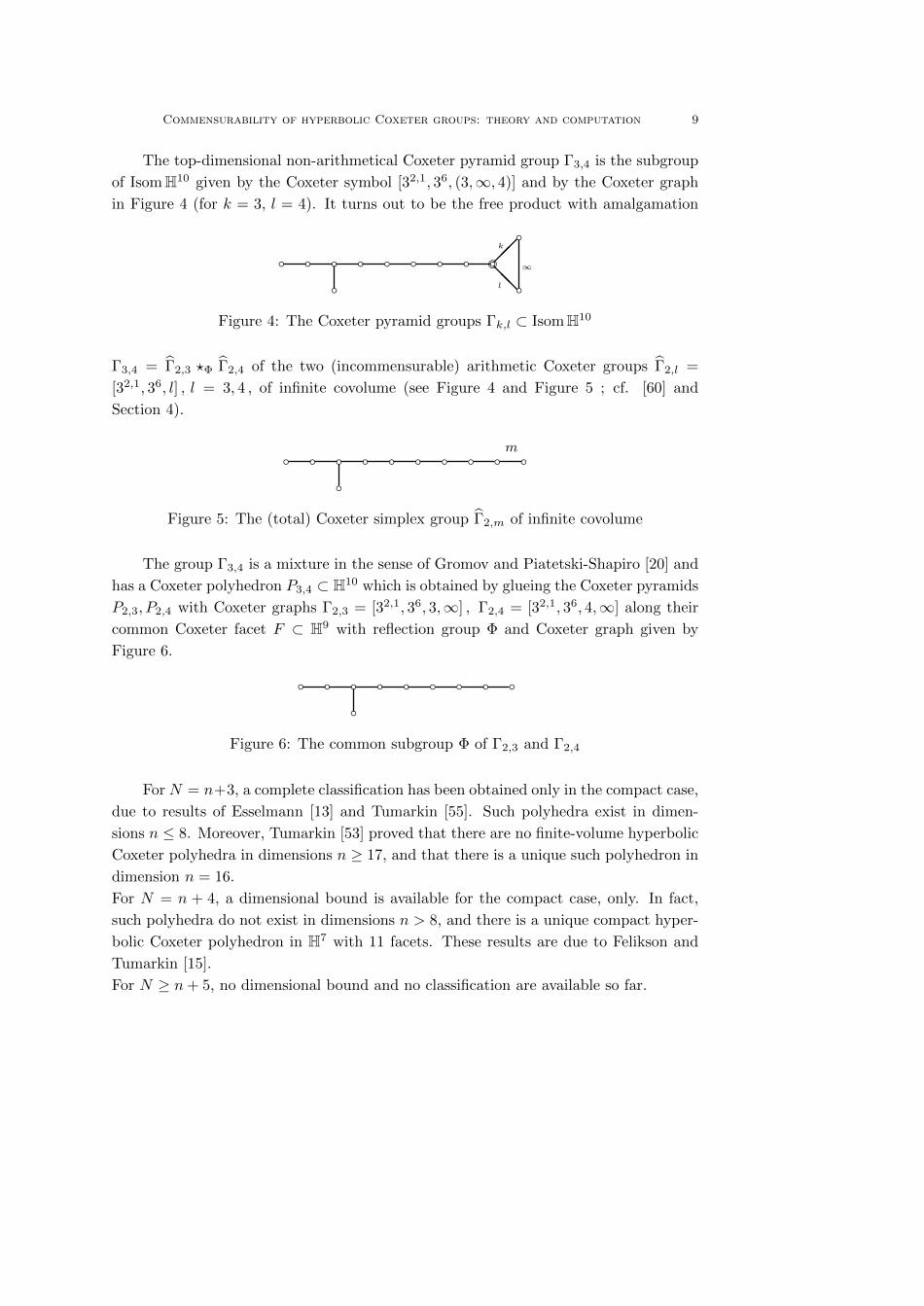
The top-dimensional non-arithmetical Coxeter pyramid group Γ3,4 is the subgroup
of IsomH10 given by the Coxeter symbol [32,1, 36, (3,∞, 4)] and by the Coxeter graph
in Figure 4 (for k = 3, l = 4). It turns out to be the free product with amalgamation
b b b b b b b b b bd bb
@@
k
l
∞
Figure 4: The Coxeter pyramid groups Γk,l ⊂ IsomH10
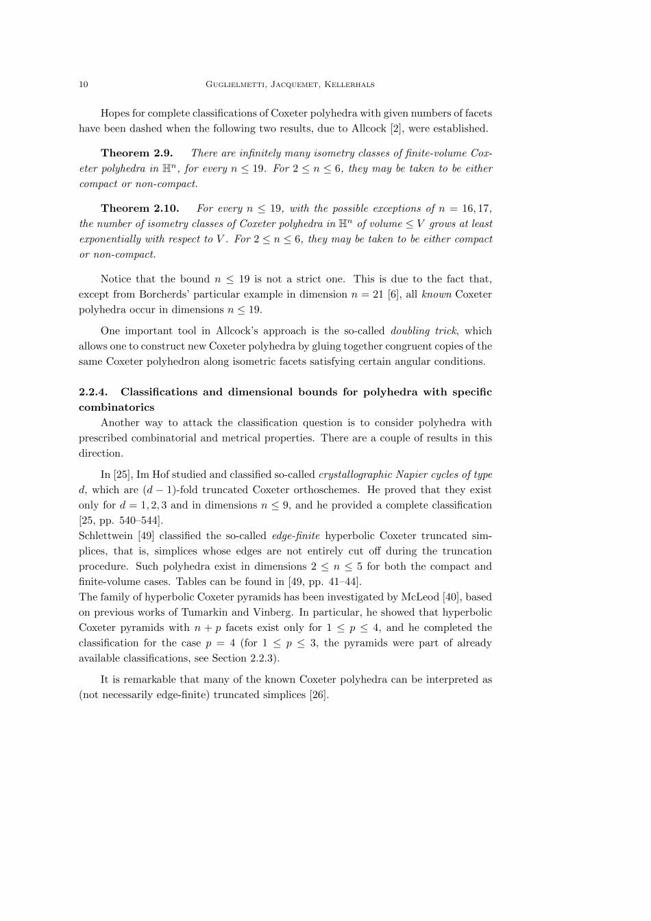
Γ3,4 = Γ2,3 ?Φ Γ2,4 of the two (incommensurable) arithmetic Coxeter groups Γ2,l =
[32,1, 36, l] , l = 3, 4 , of infinite covolume (see Figure 4 and Figure 5 ; cf. [60] and
Section 4).
b b b b b b b b b bbm
Figure 5: The (total) Coxeter simplex group Γ2,m of infinite covolume
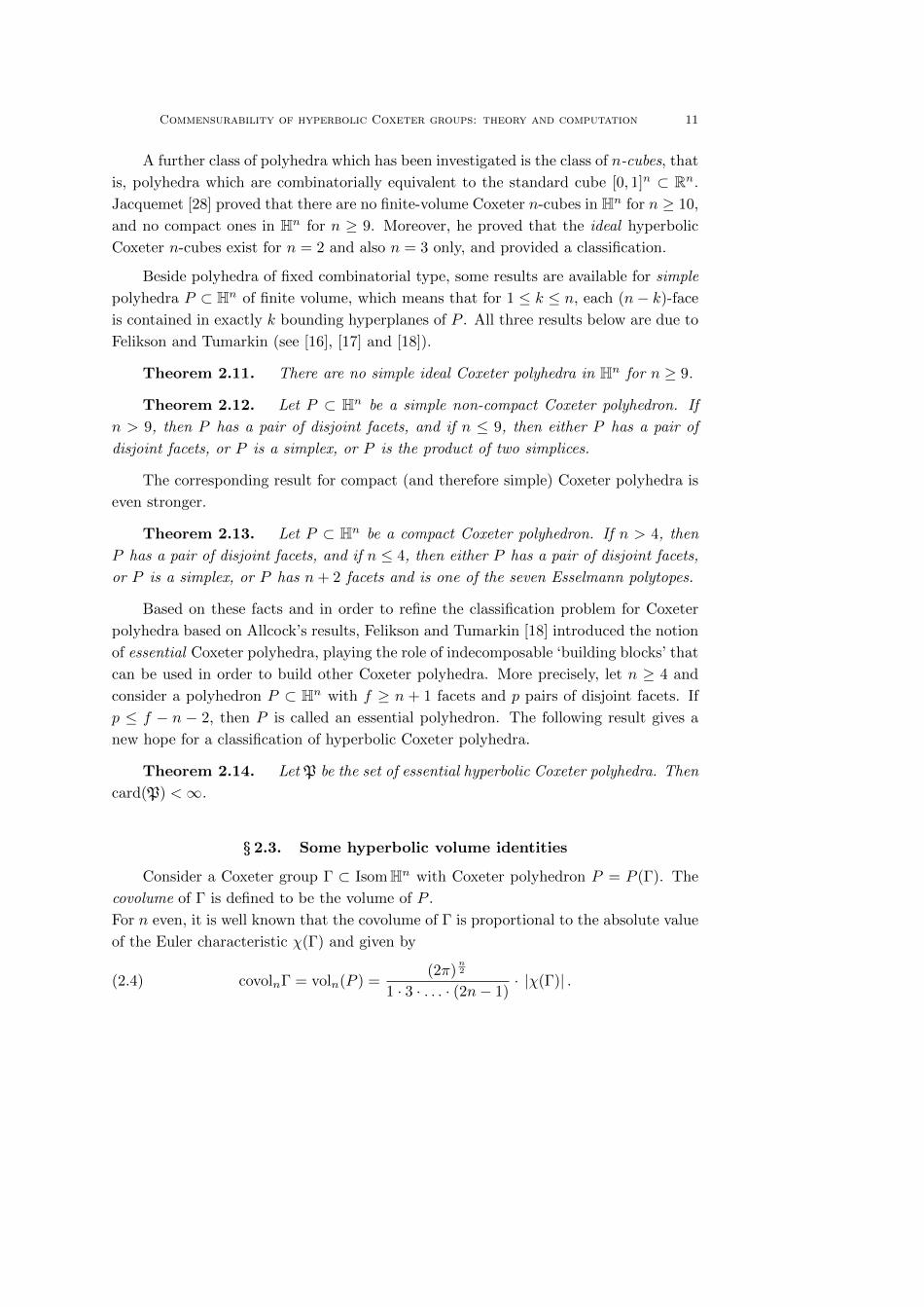
The group Γ3,4 is a mixture in the sense of Gromov and Piatetski-Shapiro [20] and
has a Coxeter polyhedron P3,4 ⊂ H10 which is obtained by glueing the Coxeter pyramids
P2,3, P2,4 with Coxeter graphs Γ2,3 = [32,1, 36, 3,∞] , Γ2,4 = [32,1, 36, 4,∞] along their
common Coxeter facet F ⊂ H9 with reflection group Φ and Coxeter graph given by
Figure 6.
b b b b b b b b bbFigure 6: The common subgroup Φ of Γ2,3 and Γ2,4
For N = n+3, a complete classification has been obtained only in the compact case,
due to results of Esselmann [13] and Tumarkin [55]. Such polyhedra exist in dimen-
sions n ≤ 8. Moreover, Tumarkin [53] proved that there are no finite-volume hyperbolic
Coxeter polyhedra in dimensions n ≥ 17, and that there is a unique such polyhedron in
dimension n = 16.
For N = n + 4, a dimensional bound is available for the compact case, only. In fact,
such polyhedra do not exist in dimensions n > 8, and there is a unique compact hyper-
bolic Coxeter polyhedron in H7 with 11 facets. These results are due to Felikson and
Tumarkin [15].
For N ≥ n+ 5, no dimensional bound and no classification are available so far.
10 Guglielmetti, Jacquemet, Kellerhals
Hopes for complete classifications of Coxeter polyhedra with given numbers of facets
have been dashed when the following two results, due to Allcock [2], were established.
Theorem 2.9. There are infinitely many isometry classes of finite-volume Cox-
eter polyhedra in Hn, for every n ≤ 19. For 2 ≤ n ≤ 6, they may be taken to be either
compact or non-compact.
Theorem 2.10. For every n ≤ 19, with the possible exceptions of n = 16, 17,
the number of isometry classes of Coxeter polyhedra in Hn of volume ≤ V grows at least
exponentially with respect to V . For 2 ≤ n ≤ 6, they may be taken to be either compact
or non-compact.
Notice that the bound n ≤ 19 is not a strict one. This is due to the fact that,
except from Borcherds’ particular example in dimension n = 21 [6], all known Coxeter
polyhedra occur in dimensions n ≤ 19.
One important tool in Allcock’s approach is the so-called doubling trick, which
allows one to construct new Coxeter polyhedra by gluing together congruent copies of the
same Coxeter polyhedron along isometric facets satisfying certain angular conditions.
2.2.4. Classifications and dimensional bounds for polyhedra with specific
combinatorics
Another way to attack the classification question is to consider polyhedra with
prescribed combinatorial and metrical properties. There are a couple of results in this
direction.
In [25], Im Hof studied and classified so-called crystallographic Napier cycles of type
d, which are (d − 1)-fold truncated Coxeter orthoschemes. He proved that they exist
only for d = 1, 2, 3 and in dimensions n ≤ 9, and he provided a complete classification
[25, pp. 540–544].
Schlettwein [49] classified the so-called edge-finite hyperbolic Coxeter truncated sim-
plices, that is, simplices whose edges are not entirely cut off during the truncation
procedure. Such polyhedra exist in dimensions 2 ≤ n ≤ 5 for both the compact and
finite-volume cases. Tables can be found in [49, pp. 41–44].
The family of hyperbolic Coxeter pyramids has been investigated by McLeod [40], based
on previous works of Tumarkin and Vinberg. In particular, he showed that hyperbolic
Coxeter pyramids with n + p facets exist only for 1 ≤ p ≤ 4, and he completed the
classification for the case p = 4 (for 1 ≤ p ≤ 3, the pyramids were part of already
available classifications, see Section 2.2.3).
It is remarkable that many of the known Coxeter polyhedra can be interpreted as
(not necessarily edge-finite) truncated simplices [26].
Commensurability of hyperbolic Coxeter groups: theory and computation 11
A further class of polyhedra which has been investigated is the class of n-cubes, that
is, polyhedra which are combinatorially equivalent to the standard cube [0, 1]n ⊂ Rn.
Jacquemet [28] proved that there are no finite-volume Coxeter n-cubes in Hn for n ≥ 10,
and no compact ones in Hn for n ≥ 9. Moreover, he proved that the ideal hyperbolic
Coxeter n-cubes exist for n = 2 and also n = 3 only, and provided a classification.
Beside polyhedra of fixed combinatorial type, some results are available for simple
polyhedra P ⊂ Hn of finite volume, which means that for 1 ≤ k ≤ n, each (n− k)-face
is contained in exactly k bounding hyperplanes of P . All three results below are due to
Felikson and Tumarkin (see [16], [17] and [18]).
Theorem 2.11. There are no simple ideal Coxeter polyhedra in Hn for n ≥ 9.
Theorem 2.12. Let P ⊂ Hn be a simple non-compact Coxeter polyhedron. If
n > 9, then P has a pair of disjoint facets, and if n ≤ 9, then either P has a pair of
disjoint facets, or P is a simplex, or P is the product of two simplices.
The corresponding result for compact (and therefore simple) Coxeter polyhedra is
even stronger.
Theorem 2.13. Let P ⊂ Hn be a compact Coxeter polyhedron. If n > 4, then
P has a pair of disjoint facets, and if n ≤ 4, then either P has a pair of disjoint facets,
or P is a simplex, or P has n+ 2 facets and is one of the seven Esselmann polytopes.
Based on these facts and in order to refine the classification problem for Coxeter
polyhedra based on Allcock’s results, Felikson and Tumarkin [18] introduced the notion
of essential Coxeter polyhedra, playing the role of indecomposable ‘building blocks’ that
can be used in order to build other Coxeter polyhedra. More precisely, let n ≥ 4 and
consider a polyhedron P ⊂ Hn with f ≥ n + 1 facets and p pairs of disjoint facets. If
p ≤ f − n − 2, then P is called an essential polyhedron. The following result gives a
new hope for a classification of hyperbolic Coxeter polyhedra.
Theorem 2.14. Let P be the set of essential hyperbolic Coxeter polyhedra. Then
card(P) <∞.
§ 2.3. Some hyperbolic volume identities
Consider a Coxeter group Γ ⊂ IsomHn with Coxeter polyhedron P = P (Γ). The
covolume of Γ is defined to be the volume of P .
For n even, it is well known that the covolume of Γ is proportional to the absolute value
of the Euler characteristic χ(Γ) and given by
(2.4) covolnΓ = voln(P ) =(2π)
n2
1 · 3 · . . . · (2n− 1)· |χ(Γ)| .
12 Guglielmetti, Jacquemet, Kellerhals
The program CoxIter developped by Guglielmetti [22] provides the value of χ(Γ), and
therefore the covolume of Γ in the even-dimensional case, for a group Γ with prescribed
Coxeter graph. More concretely, the program gives the combinatorial structure in terms
of the f -vector of P = P (Γ), whose k-th component is the number of k-faces of P . It
also allows one to decide whether Γ is cocompact or cofinite and whether it is arithmetic
(see Section 4).
For n odd, volume computations are much more difficult to handle due to the lack of
closed formulas and the implication of transcendental functions such as polylogarithms.
Let us consider some simple cases when n = 3. It is known that hyperbolic volume
can be expressed in terms of the Lobachevsky function L(ω) which is related to the
dilogarithm function Li2(z) =∑∞k=1
zk
k2 by means of
L(ω) =1
2
∞∑r=1
sin(2rω)
r2= −
ω∫0
log | 2 sin t | dt , ω ∈ R .(2.5)
The Lobachevsky function satisfies the following three essential functional properties.
• L(x) is odd.
• L(x) is π-periodic.
• L(x) satisfies for each integer m 6= 0 the distribution law
(2.6) L(mx) = m ·m−1∑k=0
L(x+kπ
m) .
In this context, let us mention the following conjectures of Milnor [51, Chapter 7], [43].
Conjectures (Milnor).
(A) Every rational linear relation between the real numbers L(x) with x ∈ Qπ is a
consequence of the three essential functional equations above.
(B) Fixing some denominator N ≥ 3, the real numbers L(kπ/N) with k relatively
prime to N and 0 < k < N/2 are linearly independent over Q.
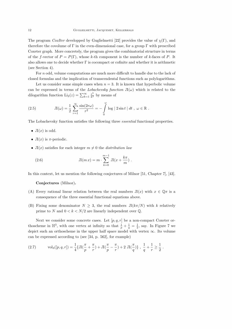
Next we consider some concrete cases. Let [p, q, r] be a non-compact Coxeter or-
thoscheme in H3, with one vertex at infinity so that 1p + 1
q = 12 , say. In Figure 7 we
depict such an orthoscheme in the upper half space model with vertex ∞. Its volume
can be expressed according to (see [34, p. 562], for example)
(2.7) vol3([p, q, r]) =1
4L(
π
p+π
r) + L(
π
p− π
r) + 2 L(
π
q) , 1
q+
1
r≥ 1
2.

Commensurability of hyperbolic Coxeter groups: theory and computation 13
Figure 7: The Coxeter orthoscheme [p, q, r] ⊂ H3 with 1p + 1
q = 12
In particular, the volumes of the Coxeter orthoschemes [3, 3, 6] and [3, 4, 4] are given by
(2.8)vol3([3, 3, 6]) =
1
8L(
π
3) ' 0.04229 ,
vol3([3, 4, 4]) =1
6L(
π
4) ' 0.07633 .
Remark. In [1] and based on Meyerhoff’s work [42], Adams proved that the 1-
cusped 3-orbifold H3/[3, 3, 6] is the (unique) non-compact hyperbolic orbifold of minimal
volume.
Consider an ideal hyperbolic tetrahedron S∞ = S∞(α, β, γ) ⊂ H3 which is char-
acterised by the dihedral angles α, β, γ ∈]0, π2 ], each one sitting at a pair of opposite
edges, and satisfying α + β + γ = π. It can be decomposed into 3 isometric pairs of
orthoschemes, each having 2 vertices at infinity, in such a way that the identity (2.7)
provides the following volume formula.
(2.9) vol3(S∞) = L(α) + L(β) + L(γ) , α+ β + γ = π .
As a consequence, a regular ideal tetrahedron S∞, characterised by α = β = γ = π3 , is
of volume 3L(π3 ). In [30], the covolumes of all hyperbolic Coxeter n-simplex groups,
3 ≤ n ≤ 9, were determined; for the values in the case of n = 3, see Appendix Appendix
A.
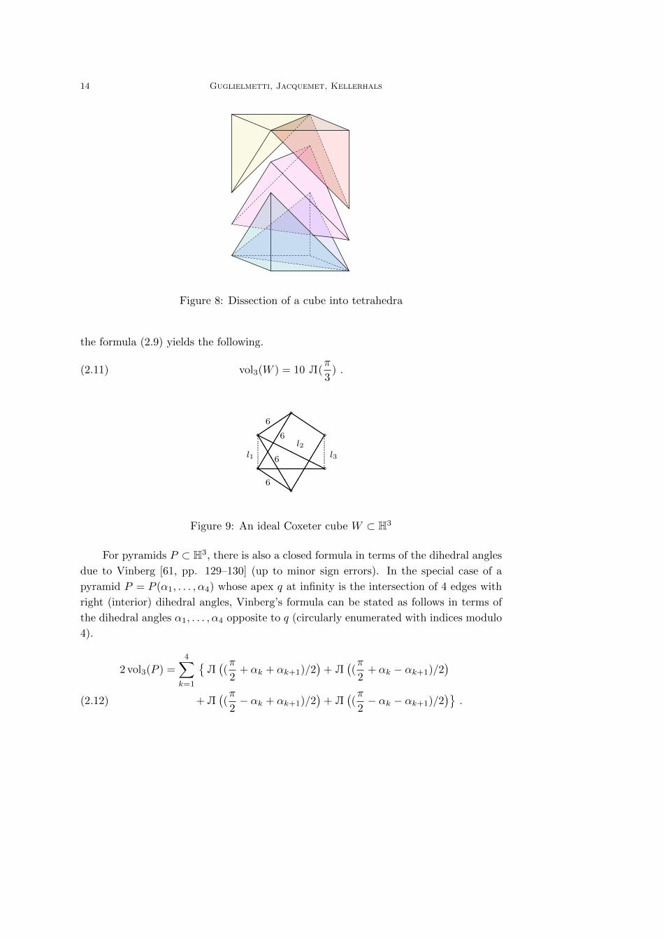
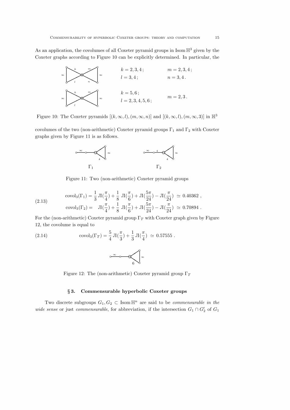
Next, consider one of the 7 ideal Coxeter cubes in H3 (see [28]). It can be dissected
into 4 ideal tetrahedra according to Figure 8. In the case of the Coxeter cube W with
Coxeter graph given by Figure 9 and edge lengths l1, l2, l3 of pairs of opposite facets
satisfying
(2.10) cosh l1 = cosh l2 =5
2, cosh l3 =
2√
3
3,
14 Guglielmetti, Jacquemet, Kellerhals
Figure 8: Dissection of a cube into tetrahedra
the formula (2.9) yields the following.
(2.11) vol3(W ) = 10 L(π
3) .
a a aa a a
QQQ
TTTTT
Q
HHHH
HH6
6
6
6l1 l3
l2
Figure 9: An ideal Coxeter cube W ⊂ H3
For pyramids P ⊂ H3, there is also a closed formula in terms of the dihedral angles
due to Vinberg [61, pp. 129–130] (up to minor sign errors). In the special case of a
pyramid P = P (α1, . . . , α4) whose apex q at infinity is the intersection of 4 edges with
right (interior) dihedral angles, Vinberg’s formula can be stated as follows in terms of
the dihedral angles α1, . . . , α4 opposite to q (circularly enumerated with indices modulo
4).
2 vol3(P ) =
4∑k=1
L((π
2+ αk + αk+1)/2
)+ L
((π
2+ αk − αk+1)/2
)+L
((π
2− αk + αk+1)/2
)+ L
((π
2− αk − αk+1)/2
).(2.12)
Commensurability of hyperbolic Coxeter groups: theory and computation 15
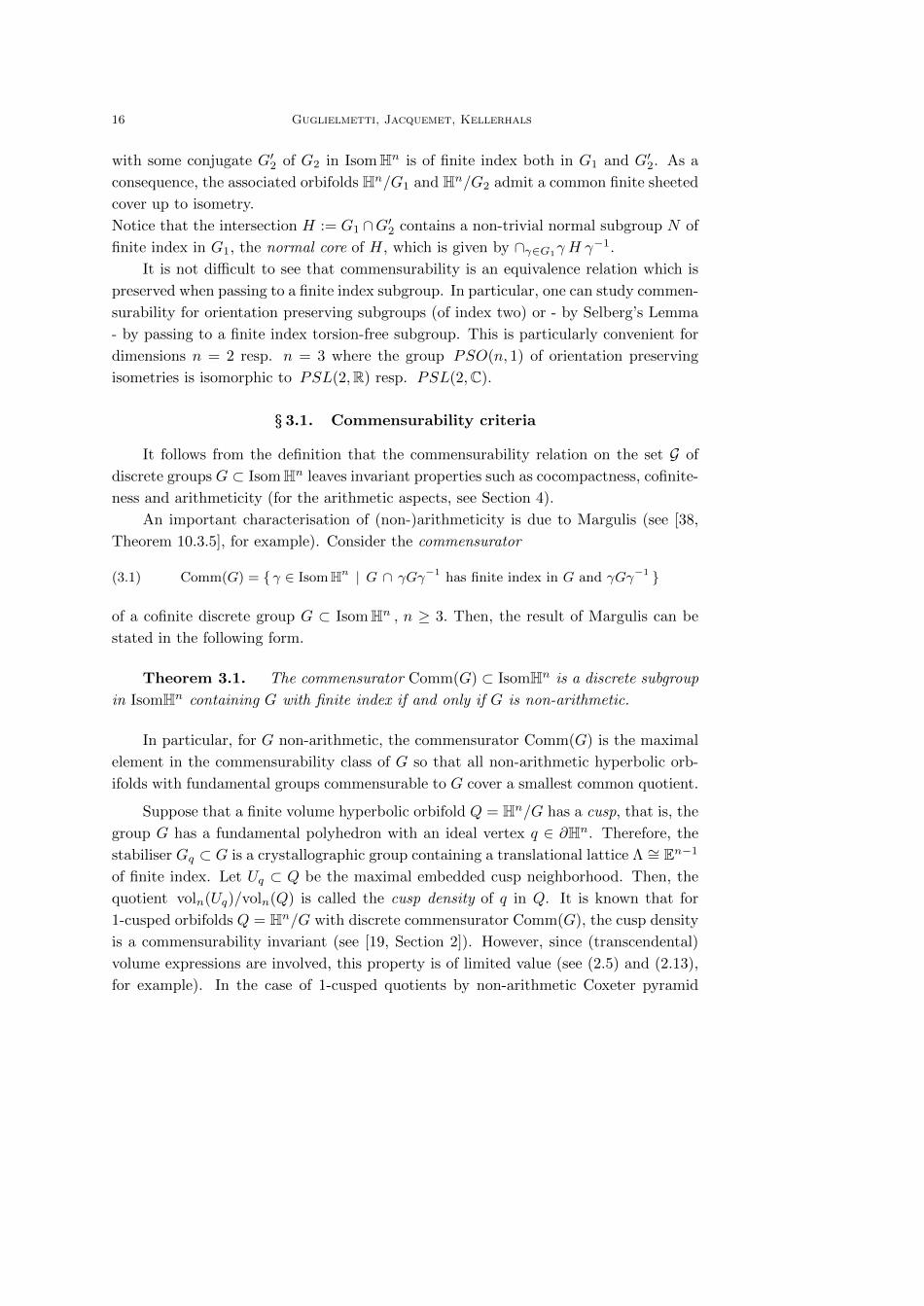
As an application, the covolumes of all Coxeter pyramid groups in IsomH3 given by the
Coxeter graphs according to Figure 10 can be explicitly determined. In particular, the
b bb bbdb bb bbd
HHH
HHH
HHH
HHH
∞ ∞
∞ ∞
k = 2, 3, 4 ;
l = 3, 4 ;
k = 5, 6 ;
l = 2, 3, 4, 5, 6 ;
m = 2, 3, 4 ;
n = 3, 4 .
m = 2, 3 .k
l
m
k
l
m
n
Figure 10: The Coxeter pyramids [(k,∞, l), (m,∞, n)] and [(k,∞, l), (m,∞, 3)] in H3
covolumes of the two (non-arithmetic) Coxeter pyramid groups Γ1 and Γ2 with Coxeter
graphs given by Figure 11 is as follows.
b b be bb4
Γ1 Γ2
b b be bb
QQ QQ
4
4∞ ∞∞ ∞
Figure 11: Two (non-arithmetic) Coxeter pyramid groups
covol3(Γ1) =1
3L(
π
4) +
1
8L(
π
6) + L(
5π
24)−L(
π
24) ' 0.40362 ,
covol3(Γ2) = L(π
4) +
1
8L(
π
6) + L(
5π
24)−L(
π
24) ' 0.70894 .
(2.13)
For the (non-arithmetic) Coxeter pyramid group ΓT with Coxeter graph given by Figure
12, the covolume is equal to
(2.14) covol3(ΓT ) =5
4L(
π
3) +
1
3L(
π
4) ' 0.57555 .
b b be bbQQ
∞∞
6
Figure 12: The (non-arithmetic) Coxeter pyramid group ΓT
§ 3. Commensurable hyperbolic Coxeter groups
Two discrete subgroups G1, G2 ⊂ IsomHn are said to be commensurable in the
wide sense or just commensurable, for abbreviation, if the intersection G1 ∩ G′2 of G1
16 Guglielmetti, Jacquemet, Kellerhals
with some conjugate G′2 of G2 in IsomHn is of finite index both in G1 and G′2. As a
consequence, the associated orbifolds Hn/G1 and Hn/G2 admit a common finite sheeted
cover up to isometry.
Notice that the intersection H := G1 ∩G′2 contains a non-trivial normal subgroup N of
finite index in G1, the normal core of H, which is given by ∩γ∈G1γ H γ−1.
It is not difficult to see that commensurability is an equivalence relation which is
preserved when passing to a finite index subgroup. In particular, one can study commen-
surability for orientation preserving subgroups (of index two) or - by Selberg’s Lemma
- by passing to a finite index torsion-free subgroup. This is particularly convenient for
dimensions n = 2 resp. n = 3 where the group PSO(n, 1) of orientation preserving
isometries is isomorphic to PSL(2,R) resp. PSL(2,C).
§ 3.1. Commensurability criteria
It follows from the definition that the commensurability relation on the set G of
discrete groups G ⊂ IsomHn leaves invariant properties such as cocompactness, cofinite-
ness and arithmeticity (for the arithmetic aspects, see Section 4).
An important characterisation of (non-)arithmeticity is due to Margulis (see [38,
Theorem 10.3.5], for example). Consider the commensurator
(3.1) Comm(G) = γ ∈ IsomHn | G ∩ γGγ−1 has finite index in G and γGγ−1
of a cofinite discrete group G ⊂ IsomHn , n ≥ 3. Then, the result of Margulis can be
stated in the following form.
Theorem 3.1. The commensurator Comm(G) ⊂ IsomHn is a discrete subgroup
in IsomHn containing G with finite index if and only if G is non-arithmetic.
In particular, for G non-arithmetic, the commensurator Comm(G) is the maximal
element in the commensurability class of G so that all non-arithmetic hyperbolic orb-
ifolds with fundamental groups commensurable to G cover a smallest common quotient.
Suppose that a finite volume hyperbolic orbifold Q = Hn/G has a cusp, that is, the
group G has a fundamental polyhedron with an ideal vertex q ∈ ∂Hn. Therefore, the
stabiliser Gq ⊂ G is a crystallographic group containing a translational lattice Λ ∼= En−1
of finite index. Let Uq ⊂ Q be the maximal embedded cusp neighborhood. Then, the
quotient voln(Uq)/voln(Q) is called the cusp density of q in Q. It is known that for
1-cusped orbifolds Q = Hn/G with discrete commensurator Comm(G), the cusp density
is a commensurability invariant (see [19, Section 2]). However, since (transcendental)
volume expressions are involved, this property is of limited value (see (2.5) and (2.13),
for example). In the case of 1-cusped quotients by non-arithmetic Coxeter pyramid
Commensurability of hyperbolic Coxeter groups: theory and computation 17
groups (see Section 5.3), we present results whose proofs are based on a different rea-
soning without volume computation but using crystallography (see Theorem 5.4 and
Lemma 5.6).
In fact, volume considerations rarely help to judge about commensurability in a
rigorous way but relate such questions to analytical number theory. As a general prin-
ciple, if the covolume quotient of two groups in G is an irrational number, then the
groups cannot be commensurable. However, already for n = 3, such criteria are very
difficult to handle and closely related to Milnor’s Conjectures presented in Section 2.3.
Furthermore, for n = 2k, the above observation is void in view of (2.4).
A natural conjugacy invariant is the (ordinary) trace field Tr(G) of G in GL(n +
1,R) which is defined to be the field generated by all the traces of matrices in G ⊂PO(n, 1). In the particular case of Kleinian groups, that is, of cofinite discrete groups
G ⊂ PSL(2,C), one can sometimes avoid trace computations by considering the in-
variant trace field kG = Q(Tr(G(2))), generated by the traces of all squared elements
γ2 , γ ∈ G , and the invariant quaternion algebra AG over kG. Both, the field kG and
the algebra AG are commensurability invariants (see [44]). Furthermore, kG is a finite
non-real extension of Q (see [38, Theorem 3.3.7]), and if the group G is not cocompact
(containing parabolic elements), then the algebra AG is isomorphic to the matrix alge-
bra Mat(2, kG) (see [38, Theorem 3.3.8]).
In the case when the group G is an amalgamated free product of the form G = G1?HG2,
where H is a non-elementary Kleinian group, then kG is a composite of fields according
to (see [38, Theorem 5.6.1])
kG = kG1 · kG2 .
In this context, consider hyperbolic Coxeter groups Γ ⊂ IsomHn which are amalgamated
free products Γ1 ?Φ Γ2 such that Φ ⊂ IsomHn−1 is itself a cofinite Coxeter group whose
fundamental Coxeter polyhedron F is a common facet of the fundamental Coxeter
polyhedra P1 and P2 of Γ1 and Γ2 (for an example, see the groups Γk,l ⊂ IsomH10 as
described by Figures 4, 5 and 6 and the explanation given in Section 2.2). Geometrically,
a fundamental polyhedron for Γ1 ?Φ Γ2 is the Coxeter polyhedron arising by glueing
together P1 and P2 along their common facet F . Then, the following general result of
Karrass and Solitar [33, Theorem 10] is very useful to decide about commensurability,
in particular in the case of Tumarkin’s Coxeter pyramid groups (for details, see Section
5.3, Lemma 5.6).
Theorem 3.2. Let G = A?U B be a free product with amalgamated subgroup U ,
and let H be a finitely generated subgroup of G containing a normal subgroup N of G
such that N ≮ U . Then, H is of finite index in G if and only if the intersection of U
with each conjugate of H is of finite index in U .
18 Guglielmetti, Jacquemet, Kellerhals
§ 4. Arithmetical aspects
In [36], Maclachlan described an effective way to decide about the commensurability
of two arithmetic discrete subgroups of IsomHn. The key point is that the classification
of arithmetic hyperbolic groups is equivalent to the classification of their underlying
quadratic forms up to similarity. In turn, the classification of these quadratic forms can
be achieved using a complete set of invariants based on quaternion algebras. In this
section, we present the necessary algebraic background, discuss the result of Maclachlan
and provide a few examples. In Appendix Appendix C we provide the commensurability
classes of arithmetic hyperbolic Coxeter pyramid groups.
§ 4.1. Arithmetic groups
In order to motivate the precise definition of an arithmetic group (of the simplest
type), we start with an example. Let fn(x) = x21 + . . . + x2
n − x2n+1 be the standard
Lorentzian quadratic form on Rn+1 and consider the cone C = x ∈ Rn+1 | fn(x) < 0.We denote by O(fn,Z) ⊂ GL(n + 1,R) the group of linear transformations of Rn+1
with coefficients in Z which preserve the quadratic form fn. The index two subgroup
O+(fn,Z) consisting of elements of O(fn,Z) which preserve the two connected compo-
nents C± = x ∈ C |xn+1 ≶ 0 of the cone C is the prototype of an arithmetic group.
Moreover, it is well known that this discrete group has finite covolume in O+(n, 1).
Note that the condition that the transformation has coefficients in Z is equivalent to
invariance requirement of the standard Z-lattice in Rn+1.
Now, let K be any totally real number field, OK its ring of integers, and let V be
an (n+ 1)-dimensional vector space over K endowed with an admissible quadratic form
f of signature (n, 1), that is, all conjugates fσ of f by the non-trivial Galois embedding
σ : K −→ R are positive definite. The cone Cf = x ∈ V ⊗ R : f(x) < 0 has
two connected components C±f and gives rise to the Minkowski model C+f /R∗ of the
hyperbolic n-space Hn. We now let
O(f) =T ∈ GL(V ⊗ R) | f T (x) = f(x), ∀x ∈ V ⊗ R
.
Finally, for a OK-lattice L of full rank in V and for O(f)K the K-points of O(f), we
consider the group
O(f, L) :=T ∈ O(f)K |T (C+
f ) = C+f , T (L) = L
.
It is a discrete subgroup of IsomHn of finite covolume (see [7]).
Definition 4.1. A discrete group Γ ⊂ IsomHn is an arithmetic group of the
simplest type if there exist K, f and L as above such that Γ is commensurable to
O(f, L). In this setting, we say that Γ is defined over K and that f is the quadratic
form associated to Γ.

Commensurability of hyperbolic Coxeter groups: theory and computation 19
Remarks 4.2 ([61, Chapter 6]).
1. If such a group is non-cocompact, then it must be defined over Q.
2. If Γ is defined over Q, then it is non-cocompact if and only if the lattice is isotropic
(see also [20, Section 2.3]). In particular, if Γ is non-compact then n ≥ 4 (this
follows from [9, Chapter 4, Lemma 2.7] and the Hasse-Minkowski theorem).
3. There is a slightly more general definition of discrete arithmetic subgroups of
IsomHn. However, when a discrete subgroup of IsomHn is arithmetic and contains
reflections, then it is of the simplest type. Therefore, we will refer to arithmetic of
group of the simplest type as arithmetic group.
Vinberg presented in [61] a criterion to decide whether a hyperbolic Coxeter group
is arithmetic or not. In order to present the criterion, we need the following definition.
Definition 4.3. Let A := (Ai,j) ∈ Mat(n,K) be a square matrix with coeffi-
cients in a field K. A cycle of length k, or k-cycle, in A is a product Ai1,i2 ·Ai2,i3 · . . . ·Aik−1,ik ·Aik,i1 . Such a cycle is denoted by A(i1,...,ik). If the ij are all distinct, the cycle
is called irreducible.
Theorem 4.4. Let Γ be a hyperbolic Coxeter group of finite covolume in IsomHn
and let G be its Gram matrix. Let K be the field generated by the entries of G and let
K be the field generated by the (irreducible) cycles in 2G. Then, Γ is arithmetic if and
only if
• K is a totally real number field;
• for each Galois embedding σ : K −→ R with σ|K 6= id, the matrix Gσ is positive
semi-definite;
• the cycles in 2G are algebraic integers in K.
In this case, the field of definition of Γ is K.
If the group Γ is a non-cocompact hyperbolic Coxeter group, then the criterion can
be simplified as follows.
Proposition 4.5 ([22, Proposition 1.13]). Let Γ = 〈s1, . . . , sN 〉 be a non-co-
compact hyperbolic Coxeter group of finite covolume, G its Gram matrix and Σ its
Coxeter graph. Then, Γ is arithmetic if and only if the two following conditions are
satisfied.
1. The graph Σ contains only edges with labels in ∞, 2, 3, 4, 6 and dotted edges.
20 Guglielmetti, Jacquemet, Kellerhals
2. 4 ·G2i,j ∈ Z.
3. For every simple cycle (si1 , . . . , sik , si1) in the graph Σ, the product(2G)
(i1,...,ik)
is a rational integer. Moreover, it is sufficient to test this condition in the graph
obtained by collapsing every non-closed path.
Remark. The condition 4 ·G2i,j ∈ Z (which must hold for a non-cocompact arith-
metic Coxeter group) is a strong condition for the weights of the dotted lines.
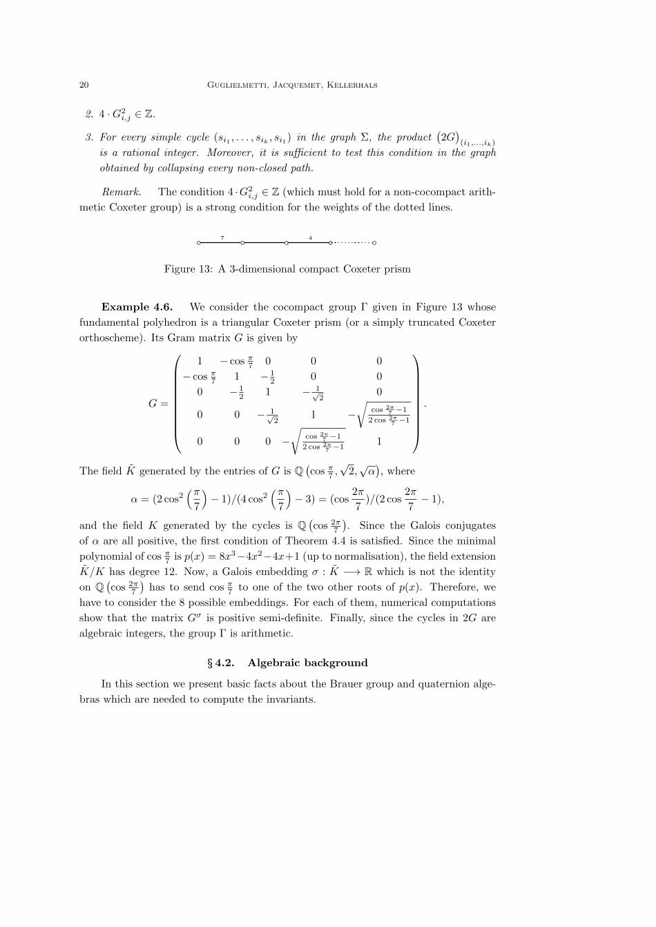
b b b b b7 4
Figure 13: A 3-dimensional compact Coxeter prism
Example 4.6. We consider the cocompact group Γ given in Figure 13 whose
fundamental polyhedron is a triangular Coxeter prism (or a simply truncated Coxeter
orthoscheme). Its Gram matrix G is given by
G =
1 − cos π7 0 0 0
− cos π7 1 − 12 0 0
0 − 12 1 − 1√
20
0 0 − 1√2
1 −√
cos 2π7 −1
2 cos 2π7 −1
0 0 0 −√
cos 2π7 −1
2 cos 2π7 −1
1
.
The field K generated by the entries of G is Q(cos π7 ,
√2,√α), where
α = (2 cos2(π
7
)− 1)/(4 cos2
(π7
)− 3) = (cos
2π
7)/(2 cos
2π
7− 1),
and the field K generated by the cycles is Q(cos 2π
7
). Since the Galois conjugates
of α are all positive, the first condition of Theorem 4.4 is satisfied. Since the minimal
polynomial of cos π7 is p(x) = 8x3−4x2−4x+1 (up to normalisation), the field extension
K/K has degree 12. Now, a Galois embedding σ : K −→ R which is not the identity
on Q(cos 2π
7
)has to send cos π7 to one of the two other roots of p(x). Therefore, we
have to consider the 8 possible embeddings. For each of them, numerical computations
show that the matrix Gσ is positive semi-definite. Finally, since the cycles in 2G are
algebraic integers, the group Γ is arithmetic.
§ 4.2. Algebraic background
In this section we present basic facts about the Brauer group and quaternion alge-
bras which are needed to compute the invariants.
Commensurability of hyperbolic Coxeter groups: theory and computation 21
4.2.1. The Brauer group Let K be a field and let A be a finite dimensional central
simple algebra over K (the center of A is K and A has no proper non-trivial two-sided
ideal). By Wedderburn’s theorem, there exists a unique (up to isomorphism) division
algebra D over K and a unique integer n such that A ∼= Mat(n,D). This allows to define
an equivalence relation on the set of isomorphism classes of central simple algebras over
K: two algebras A ∼= Mat(n,D) and A′ ∼= Mat(n′, D′) are said to be Brauer equivalent
if and only if D ∼= D′. The quotient set is endowed with the structure of an abelian
group as follows:
[A] · [B] = [A⊗K B].
We remark that the neutral element is the class of Mat(m,K) and [A]−1 =[Aop
], where
Aop denotes the opposite algebra of A. Note that we will often write A · B instead of
[A] · [B].
The Brauer group is denoted by BrK. All its elements are torsion and the 2-torsion is
generated by quaternions algebras (see [41]).
4.2.2. Quaternion algebras Let K be a field of characteristic different of two. A
quaternion algebra over K is a four-dimensional central simple algebra over K. Since
the characteristic of K is different from two, there exist a K-basis 1, i, j, k of A and
two non-zero elements a and b of K such that the multiplication in A is given by the
following rules:
i2 = a, j2 = b, ij = −ji = k.
We then write A = (a, b)K or just (a, b) if there is no confusion about the base field.
We sometimes call (a, b)K the Hilbert symbol of the quaternion algebra. This is kind of
unfortunate because we also have the Hilbert symbol of a field K, which is the function
K∗ ×K∗ −→ −1, 1 defined as follows.
(a, b) =
1 if ax2 + by2 − z2 = 0 has a non-trivial solution in K3
−1 otherwise.
We will use this function later when speaking about the ramification of rational quater-
nion algebras.
For an element q = x + yi + zj + tk, with x, y, z, t ∈ K, the standard involution
q = x− yi− zj − tk gives rise to the norm
N : A −→ K, q 7−→ N(q) = q · q = x2 − ay2 − bz2 + abt2.
Since an element q ∈ A is invertible if and only if N(q) 6= 0, we have the following
proposition.
22 Guglielmetti, Jacquemet, Kellerhals
Proposition 4.7 ([35, Chapter III, Theorem 2.7]). Let A = (a, b)K be a quater-
nion algebra. Then, the following properties are equivalent:
• A is a division algebra;
• the norm N : A −→ K has no non-trivial zero;
• the equation aX2 + bY 2 = 1 has no solution in K ×K;
• the equation aX2 + bY 2 − Z2 = 0 has only the trivial solution.
Moreover, if A is not a division algebra, then A ∼= Mat(2;K).
Therefore, deciding whether a given quaternion algebra is a division algebra or not
reduces to a purely number theoretical question. We will come back to this question
later.
Proposition 4.8. For every a, b, c ∈ K∗, we have the following isomorphisms
of quaternion algebras:
(a, b) ∼= (b, a), (a, c2b) ∼= (a, b), (a, a) ∼= (a,−1)
(a, 1) ∼= (a,−a) ∼= (a, 1− a) ∼= (1, 1) ∼= 1
(a, b) · (a, c) ∼= (a, bc) ·Mat(2;K), (a, b)2 ∼= Mat(4;K).
We note that the last two relations can be rewritten in the Brauer group as follows
(a, bc) = (a, b) · (a, c), (a, b)2 = 1.
Proposition 4.9 ([56, chapitre I, Theoreme 2.9; chapitre III, Section 3]). If K
is a number field, and if B1 and B2 are quaternion algebras over K, there exists a
quaternion algebra B such that B1 ·B2 = B in BrK.
4.2.3. Isomorphism classes of quaternion algebras We will see below that
the question of the commensurability of two arithmetic Coxeter subgroups of IsomHn
reduces almost to deciding whether two quaternions algebras are isomorphic. Hence, in
this section, we investigate the isomorphism classes of quaternion algebras.
First, it is worth to mention that the isomorphism classes of quaternion algebras
are not determined by Hilbert symbols (for example, we have (5, 3)Q ∼= (−10, 33)Q).
However, we will see that there is an efficient way to produce a set which completely
describe the quaternion algebra: the ramification set.
Let K be a number field. Recall that a place of K is an equivalence class of absolute
values1: two non-trivial absolute values | · |1, | · |2 : K −→ R are equivalent if there exists
1Some authors use the word (multiplicative) valuation for what we call absolute value. This is whya place is often denoted by v.
Commensurability of hyperbolic Coxeter groups: theory and computation 23
some number e ∈ R such that |x|1 = |x|e2 for all x ∈ K. We can easily create two kind
of places:
Infinite places Any Galois embedding σ : K −→ R yields a place by composition
with the usual absolute value. Similarly, any complex Galois embedding σ : K −→C gives rise to a place by composition with the modulus. These places are called
infinite places.
Note that in our setting, since the number field K is supposed to be totally real,
we only get real embeddings.
Finite places Let P be a prime ideal of OK . This defines a valuation on OK as
follows:
ηP : OK −→ Z ∪ ∞, ηP(x) = supr ∈ N : x ∈ Pr.This valuation can be extended to K by setting ηP(x/y) = ηP(x) − ηP(y). Now,
we pick any 0 < λ < 1 and define the associated absolute value
| · |P : K −→ R, |x|P = ληP(x).
Note that the place associated to this absolute value is independent of the choice of
λ. The places defined in this way are called finite places.
Using Ostrowski’s theorem and theorems about extensions of absolute values, one gets
the following standard result.
Theorem 4.10. Let K be a number field. The two constructions explained above
give all the places on K.
We will denote by Ω(K) (respectively Ω∞(K) and Ωf (K)) the set of all places
(respectively infinite places and finite places) of K. If v ∈ Ω(K) is a place, we denote
by Kv the completion of K with respect to v. For a quaternion algebra B over K, we
write Bv for B⊗K Kv, which is a quaternion algebra over Kv. When the place v comes
from a prime ideal P of OK , we will sometimes write KP instead of Kv and BP instead
of Bv.
The fact that Bv is either a division algebra or a matrix algebra (see Proposition 4.7)
motivates the following definition.
Definition 4.11. Let B be a quaternion algebra defined over a number field K.
The ramification set of B, denoted by RamB, is defined as follows:
RamB =v ∈ Ω(K) |Bv := B ⊗K Kv is a division algebra
.
We will also write
Ramf B := RamB ∩ Ωf (K), Ram∞B = RamB ∩ Ω∞(K).
24 Guglielmetti, Jacquemet, Kellerhals
Theorem 4.12 ([56, Chapter III, Theorem 3.1]). Let B be a quaternion algebra
defined over a number field K. The ramification set RamB of B is a finite set of even
cardinality. Conversely, if R ⊂ Ω(K) is a finite set of even cardinality, there exists, up
to isomorphism, a unique quaternion algebra B′ over K such that RamB′ = R.
Remark. Using Proposition 4.7 it is easy to compute the infinite ramification
Ram∞B of a quaternion algebra B = (a, b)K . Indeed, if σ : K −→ R is a Galois
embedding and if v is the corresponding absolute value, then Bv ∼=(σ(a), σ(b)
). Thus,
v ∈ Ram∞(a, b)K if and only if σ(a) > 0 and σ(b) > 0.
Remark. When K = Q, the previous theorem comes from classical results such
as the Hasse-Minkowski principle (since two quaternion algebras are isomorphic if the
quadratic spaces induced by their norms are isomorphic) and Hilbert’s reciprocity law.
Finally, let us mention a result which helps for computations in the case K = Q(see also Proposition 4.15).
Proposition 4.13 ([56, p. 78]). Let B1 and B2 be two quaternion algebras over
a number field K and let B be such that B1 · B2 = B ∈ BrK (see Proposition 4.9).
Then, we have
RamB =(
RamB1 ∪ RamB2
)\(
RamB1 ∩ RamB2
).
When dealing with arithmetic groups of odd dimensions, we will need to compute
the ramification of quaternion algebras over a quadratic extension of a number field.
Proposition 4.14. Let K be a number field and let L = K(√δ) be a quadratic
extension of K. Let B be a quaternion algebra over K and define A := B ⊗K L. Then,
the ramification sets at finite places of A and B are related as follows:
Ramf A =P1,P
′1, . . . ,Pr,P
′r,
where each pair Pi,P′i is a pair of prime ideals of OL which lie above a prime ideal Pi
of OK such that B is ramified at Pi, and Pi splits completely.
Proof. Let P be a prime ideal of OL and let P := P ∩ OK . We also consider the
completions LP (respectively KP) of L (respectively K) with respect to the valuation
defined by P (respectively P). We first note that AP∼= BP ⊗KP LP. Indeed, we have
AP∼= A⊗L LP = (B ⊗K L)⊗L LP
∼= B ⊗K LP∼= BP ⊗KP LP.
By classical results, we then have three possibilities for the ideal POL:

Commensurability of hyperbolic Coxeter groups: theory and computation 25
1. Inert case The ideal POL is prime, meaning that POL = P.
2. Ramified case We have POL = P2.
3. Split case There exists another prime ideal P′ above P such that POL = PP′.
In the first two cases, [LP : KP ] = 2 (see, for example, [9, Chapter I, 5, Proposition 3])
which implies that AP is a matrix algebra (see [56, chapitre II, Theoreme 1.3]). In the
last case, we have KP ∼= LP (again by [9]) and thus AP∼= BP . Therefore, A is ramified
at P if and only if B is ramified at P if and only if A is ramified at P′, as required.
Computing the ramification set when K = Q. In this part we consider a
quaternion algebra B = (a, b) over Q, and we explain how to compute its ramification.
In this setting, the finite places are the p-adic valuations, and there is exactly one
infinite place, denoted by | · |∞, corresponding to the usual absolute value. By virtue
of Proposition 4.7, it is clear that B is ramified at ∞ if and only if a < 0 and b < 0.
Moreover, using Proposition 4.8 and Proposition 4.13, we see that we only have to
compute the ramification set for quaternion algebras which are of one of the following
forms:
(−1, q), (p, q), (−p, q), ∀p, q ∈ P,where P denotes the set of prime numbers.
Proposition 4.15. We have Ram(−1, 2) = ∅ and Ram(−1,−2) = 2,∞.If q is a prime number different from two, then we have the following ramification
sets:
q ≡ 1 mod 8 q ≡ 3 mod 8 q ≡ 5 mod 8 q ≡ 7 mod 8
(−1, q) ∅ 2, q ∅ 2, q(−1,−q) 2,∞ q,∞ 2,∞ q,∞(2,−q) ∅ 2, q 2, q ∅(−2, q) ∅ ∅ 2, q 2, q
Finally, let q1, q2 ∈ P \ 2 be two distinct prime numbers. The ramification set of the
quaternion algebra (−q1, q2) is as follows:
q2 ≡ 1 (mod 4) q2 ≡ 3 (mod 4)
q1 ≡ 1 (mod 4)q1, q2 if
(q1q2
)= −1
∅ otherwise
2, q1 if(q1q2
)= −1
2, q2 otherwise
q1 ≡ 3 (mod 4)q1, q2 if
(q1q2
)= −1
∅ otherwise
q1, q2 if(q1q2
)= 1
∅ otherwise
where(ab
)denotes the Legendre symbol of a and b.
26 Guglielmetti, Jacquemet, Kellerhals
Proof. For x, y ∈ Q we have the Hilbert symbol (x, y)p ∈ −1, 1 (see, for example,
[9]) and for a diagonal quadratic form f = 〈a1, . . . , an〉, we define
c(f)p =∏i<j
(ai, aj)p, c(B)p = c(〈1,−a,−b, ab〉
)p.
By [9, Lemme 2.6, page 59]), we get
p ∈ Ram(B)⇔ c(B)p =
1 p = 2,∞−1 p odd.
Therefore, to find the ramification set it is sufficient to compute the Hilbert symbols
c(B)p. To compute these symbols, we can use [50, Part I, Chapter III, Theorem 1]. We
note that if p ∈ RamB, then we must have p = 2 or p | a or p | b.It follows that the Hilbert symbols satisfy
c((−1, 2)
)2
= (−1,−2)2 = −1, c((−1,−2)
)2
= (2,−1)2 = 1,
c((−1, q)
)2
= (−q,−q)2 = (−1)ε(−q), c((−1, q)
)q
= (−q,−q)q = (−1)ε(q),
c((−1,−q)
)2
= (q, q)2 = (−1)ε(q), c((−1,−q)
)q
= (q, q)q = (−1)ε(q),
c((2,−q)
)q
= (−1)ω(q), c((−2, q)
)q
= (−1)ε(q)+ω(q),
c((2,−q)
)2
= (q,−1)2 · (−2,−q)2 = (−1)1+ω(−q),
c((−2, q)
)2
= (2,−1)2 · (−q,−2)2 = (−1)ε(−q)+ω(−q),
where
ε(n) =
0 if n ≡ 1 (mod 4)
1 if n ≡ 3 (mod 4), ω(n) =
0 if n ≡ ±1 (mod 8)
1 if n ≡ ±3 (mod 8).
Finally, if q1, q2 ∈ P \ 2 are two distinct prime numbers, we have
c((−q1, q2)
)2
= (q1,−1)2 · (−q2,−q1)2 = (−1)ε(q1)+ε(−q1)·ε(−q2)
c((−q1, q2)
)q1
= (q1,−1)q1 · (−q2,−q1)q1 =
(q2
q1
)c((−q1, q2)
)q2
= (q1,−1)q2 · (−q2,−q1)q2 = (−1)ε(q2) ·(q1
q2
),
where(ab
)denotes the Legendre symbol of a and b.
4.2.4. Clifford algebras In this section, we present basic facts about Clifford alge-
bras. These algebras are used to prove Maclachlan’s theorem (cf. Theorem 4.20) but
Commensurability of hyperbolic Coxeter groups: theory and computation 27
are not used for the computations of the invariants. The reader who only wants to
compute the invariants can skip this part.
Let (V, f) be a quadratic space defined over some field K. A Clifford algebra
associated to (V, f) is a unitary associative algebra over K denoted by Cl(V, f), together
with a K-linear map i : V −→ Cl(V, f) which satisfy the following:
• For every v ∈ V , i(v)2 = f(v) · 1Cl(V,f).
• The following universal property is satisfied: if A is another unitary associative K-
algebra provided with a K-linear function iA : V −→ A such that iA(v)2 = f(v)·1A,
then there exists a unique morphism of K algebras ψ : Cl(V, f) −→ A such that
the following diagram commutes.
ViA //
i
A
Cl(V, f)
ψ
;;
Because of the universal property, if the Clifford algebra Cl(V, f) exists, then it is unique
up to isomorphism. In fact, the algebra can be constructed explicitly as follows. We
start with the tensor algebra T (V ) =⊕
i∈N V⊗n, where V ⊗n = V ⊗. . .⊗V , n times, and
V ⊗0 = K. Then we consider the ideal I in T (V ) generated by the elements v2 − f(v).
Finally, we see that the quotient T (V )/I satisfies the universal property as required.
Thus, we have Cl(V, f) = T (V )/I. When working in Cl(V, f) we will abbreviate and
write the product a⊗ b in the form a · b. It is easy to see that if v1, . . . , vn is a K-basis
of V , then vi1 · . . . · vik | 1 ≤ i1 < i2 < . . . < ik ≤ n
is a K-basis of Cl(V, f). In particular, dimk Cl(V, f) = 2dimK V .
The natural N-grading on the tensor algebra T (V ) induces a(Z/2Z
)-grading on
Cl(V, f) which is compatible with the algebra structure. In other words, the vector
space
Cl0(V, f) := spanKvi1 · . . . · vik | 1 ≤ i1 < i2 < . . . < ik ≤ n, k even
is a sub-algebra of Cl(V, f) called the even part of Cl(V, f). More canonically, Cl0(V, f)
is the image of⊕
i∈N V⊗2i by the quotient map.
Example 4.16. Let V = Rn be endowed with the quadratic form f(v) = −‖v‖2,
where ‖ · ‖ is the euclidean norm. For n = 1 we have Cl(V, f) = C and for n = 2 we
get Cl(V, f) = (−1,−1)R, the quaternions of Hamilton. In the latter case, we have
Cl0(V, f) ∼= C.
28 Guglielmetti, Jacquemet, Kellerhals
Remark. In some cases, it is useful to construct the algebra by requiring v2 =
−f(v) instead of v2 = f(v). The choice depends on the authors.
§ 4.3. Classification
Let Γ1,Γ2 ⊂ IsomHn be two arithmetic Coxeter groups defined over the number
fields K1 and K2, respectively, and let f1 and f2 be their underlying quadratic forms.
A result of Gromov and Piatetski-Shapiro (see [20, Section 2.6]) implies the following
result:
Γ1 ∼ Γ2 ⇔ K1 = K2 and f1 ∼ f2,
where Γ1 ∼ Γ2 means that Γ1 and Γ2 are commensurable and where f1 ∼ f2 means that
the two quadratic forms are similar (meaning that there exists c ∈ K1 = K2 such that
c · f1∼= f2). Therefore, deciding whether Γ1 is commensurable to Γ2 can be done in two
steps. First, we have to find the defining fields and the underlying quadratic forms (see
[57, Section II, Theorem 2]). Secondly, we have to detect the similarity of the forms.
The main references for this section are [36] and [57].
Remark. An immediate consequence of the result of Gromov and Piatetski-
Shapiro is the following: when n is odd, a necessary condition for Γ1 and Γ2 to be
commensurable is that K1 = K2 and that the quotient det f1/ det f2 is a square in K1.
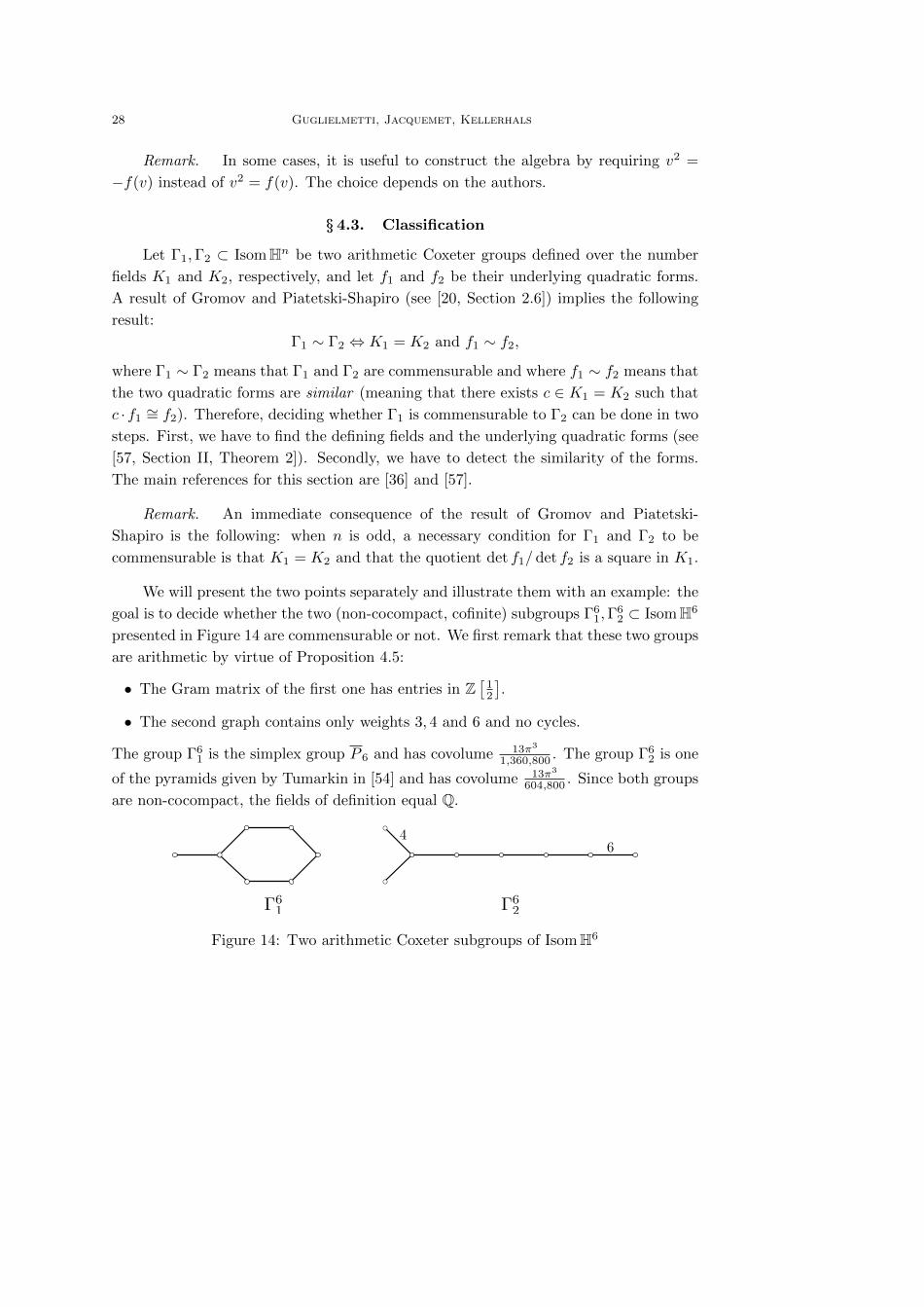
We will present the two points separately and illustrate them with an example: the
goal is to decide whether the two (non-cocompact, cofinite) subgroups Γ61,Γ
62 ⊂ IsomH6
presented in Figure 14 are commensurable or not. We first remark that these two groups
are arithmetic by virtue of Proposition 4.5:
• The Gram matrix of the first one has entries in Z[
12
].
• The second graph contains only weights 3, 4 and 6 and no cycles.
The group Γ61 is the simplex group P 6 and has covolume 13π3
1,360,800 . The group Γ62 is one
of the pyramids given by Tumarkin in [54] and has covolume 13π3
604,800 . Since both groups
are non-cocompact, the fields of definition equal Q.
Figure 14: Two arithmetic Coxeter subgroups of IsomH6
Commensurability of hyperbolic Coxeter groups: theory and computation 29
4.3.1. Finding the defining field and the underlying quadratic form Let
Γ ⊂ IsomHn be an arithmetic Coxeter group of rank N . We want to find the defining
field K and the underlying quadratic form f of Γ. We consider the associated funda-
mental polyhedron P (Γ) and the outward-pointing normal vectors ei ∈ Rn+1 of the
bounding hyperplanes Hi of P (Γ), which means that P (Γ) =⋂Ni=1H
−ei (see (2.1)). Fi-
nally, we denote by G(Γ) = (ai,j) ∈ Mat(R, N) the Gram matrix of Γ, meaning that
ai,j = 〈ei, ej〉.Using Vinberg’s arithmeticity Criterion (see Theorem 4.4), we can determine the defin-
ing field K of Γ. Now, consider the K-subvector space V spanned by all the vectors
(4.1) vi1,...,ik = a1,i1 · ai1,i2 · . . . · aik−1,ikeik , i1, . . . , ik ⊂ 1, . . . , N.
The restriction of the Lorentzian form f0 to V is an admissible quadratic space of
dimension n + 1 over K. Moreover, Γ is commensurable to O(f, L), where L is the
lattice spanned over K by a basis v1, . . . , vn+1 of V and f is the quadratic form defined
by the matrix whose entries are the Lorentzian products 〈vi, vj〉 of signature (n, 1).
Remark. The task of finding the outward-pointing normal vectors of the poly-
hedron P (Γ) is difficult: one has to find the vectors e1, . . . , eN of Rn+1 such that
〈ei, ej〉 = ai,j . This is basically equivalent to solve a system of r(r+1)2 quadratic equa-
tions with r(n+1) unknowns. Assuming that e1 = (0, . . . , 0, 1) and that the first vectors
contain a lot of zeroes, we can guess the remaining vectors using software such as Math-
ematica or Maple. Another possibility is to compute sufficiently good approximations
of the vectors ei using numerical methods and then use the LLL algorithm to find the
exact components. This approach is described in [5].
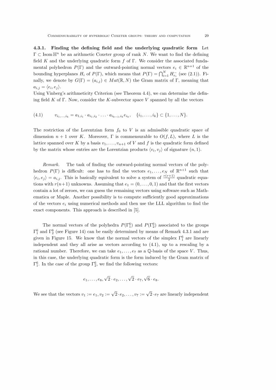
The normal vectors of the polyhedra P (Γ61) and P (Γ6
2) associated to the groups
Γ61 and Γ6
2 (see Figure 14) can be easily determined by means of Remark 4.3.1 and are
given in Figure 15. We know that the normal vectors of the simplex Γ61 are linearly
independent and they all arise as vectors according to (4.1), up to a rescaling by a
rational number. Therefore, we can take e1, . . . , e7 as a Q-basis of the space V . Thus,
in this case, the underlying quadratic form is the form induced by the Gram matrix of
Γ61. In the case of the group Γ6
2, we find the following vectors:
e1, . . . , e8,√
2 · e2, . . . ,√
2 · e7,√
6 · e8.
We see that the vectors v1 := e1, v2 :=√
2 ·e2, . . . , v7 :=√
2 ·e7 are linearly independent
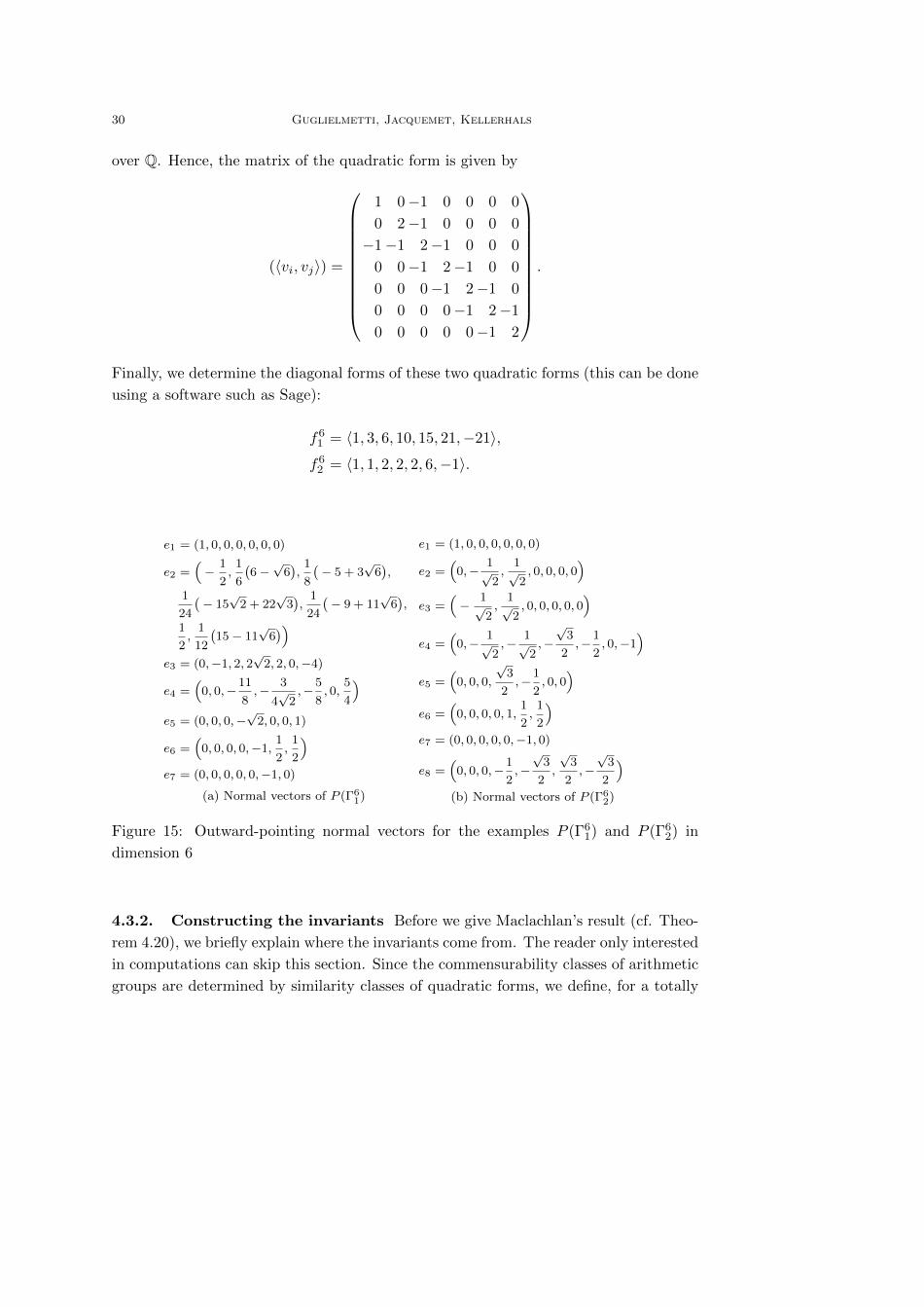
30 Guglielmetti, Jacquemet, Kellerhals
over Q. Hence, the matrix of the quadratic form is given by
(〈vi, vj〉) =
1 0−1 0 0 0 0
0 2−1 0 0 0 0
−1−1 2−1 0 0 0
0 0−1 2−1 0 0
0 0 0−1 2−1 0
0 0 0 0−1 2−1
0 0 0 0 0−1 2
.
Finally, we determine the diagonal forms of these two quadratic forms (this can be done
using a software such as Sage):
f61 = 〈1, 3, 6, 10, 15, 21,−21〉,f6
2 = 〈1, 1, 2, 2, 2, 6,−1〉.
e1 = (1, 0, 0, 0, 0, 0, 0)
e2 =(−
1
2,
1
6
(6−√
6),
1
8
(− 5 + 3
√6),
1
24
(− 15√
2 + 22√
3),
1
24
(− 9 + 11
√6),
1
2,
1
12
(15− 11
√6))
e3 = (0,−1, 2, 2√
2, 2, 0,−4)
e4 =(
0, 0,−11
8,−
3
4√
2,−
5
8, 0,
5
4
)e5 = (0, 0, 0,−
√2, 0, 0, 1)
e6 =(
0, 0, 0, 0,−1,1
2,
1
2
)e7 = (0, 0, 0, 0, 0,−1, 0)
(a) Normal vectors of P (Γ61)
e1 = (1, 0, 0, 0, 0, 0, 0)
e2 =(
0,−1√
2,
1√
2, 0, 0, 0, 0
)e3 =
(−
1√
2,
1√
2, 0, 0, 0, 0, 0
)e4 =
(0,−
1√
2,−
1√
2,−√
3
2,−
1
2, 0,−1
)e5 =
(0, 0, 0,
√3
2,−
1
2, 0, 0
)e6 =
(0, 0, 0, 0, 1,
1
2,
1
2
)e7 = (0, 0, 0, 0, 0,−1, 0)
e8 =(
0, 0, 0,−1
2,−√
3
2,
√3
2,−√
3
2
)(b) Normal vectors of P (Γ6
2)
Figure 15: Outward-pointing normal vectors for the examples P (Γ61) and P (Γ6
2) in
dimension 6
4.3.2. Constructing the invariants Before we give Maclachlan’s result (cf. Theo-
rem 4.20), we briefly explain where the invariants come from. The reader only interested
in computations can skip this section. Since the commensurability classes of arithmetic
groups are determined by similarity classes of quadratic forms, we define, for a totally
Commensurability of hyperbolic Coxeter groups: theory and computation 31
real number field K, the following map:
Θ : SimQF(K,n+ 1) −→ IsomAlg(K, 2n)[(V, f)
]7−→ Cl0(V, f),
where SimQF(K,n + 1) is the set of similarity classes of quadratic spaces over K of
dimension n+ 1, and IsomAlg(K, 2n) is the set of isomorphism classes of algebras over
K of dimension 2n. If we restrict the map Θ to the quadratic forms f of signature (n, 1)
whose conjugates fσ under non-trivial Galois embeddings σ : K −→ R are positive
definite, then we get an injective map (see [36, Theorems 6.1 and 6.2]). Hence, we have
to be able to decide whether the even parts of the Clifford algebras (see Section 4.2.4)
associated to the underlying quadratic forms are isomorphic as algebras. Luckily for
us, in this setting, there is an efficient way to decide that using the Witt and the Hasse
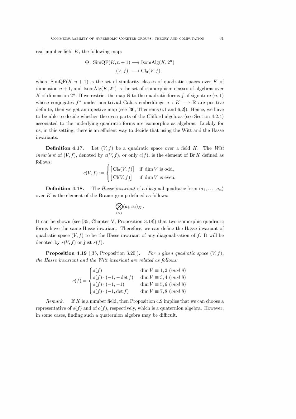
invariants.
Definition 4.17. Let (V, f) be a quadratic space over a field K. The Witt
invariant of (V, f), denoted by c(V, f), or only c(f), is the element of BrK defined as
follows:
c(V, f) :=
[
Cl0(V, f)]
if dimV is odd,[Cl(V, f)
]if dimV is even.
Definition 4.18. The Hasse invariant of a diagonal quadratic form 〈a1, . . . , an〉over K is the element of the Brauer group defined as follows:⊗
i<j
(ai, aj)K .
It can be shown (see [35, Chapter V, Proposition 3.18]) that two isomorphic quadratic
forms have the same Hasse invariant. Therefore, we can define the Hasse invariant of
quadratic space (V, f) to be the Hasse invariant of any diagonalisation of f . It will be
denoted by s(V, f) or just s(f).
Proposition 4.19 ([35, Proposition 3.20]). For a given quadratic space (V, f),
the Hasse invariant and the Witt invariant are related as follows:
c(f) =
s(f) dimV ≡ 1, 2 (mod 8)
s(f) · (−1,−det f) dimV ≡ 3, 4 (mod 8)
s(f) · (−1,−1) dimV ≡ 5, 6 (mod 8)
s(f) · (−1,det f) dimV ≡ 7, 8 (mod 8)
Remark. If K is a number field, then Proposition 4.9 implies that we can choose a
representative of s(f) and of c(f), respectively, which is a quaternion algebra. However,
in some cases, finding such a quaternion algebra may be difficult.
32 Guglielmetti, Jacquemet, Kellerhals
The even case We suppose that n is even. Let Γ be an arithmetic group defined
over a totally real number field K with underlying quadratic form f . Consider the Witt
invariant c(f) and a quaternion algebra B which represents c(f). Then, we have
Θ(f) = Cl0(f) ∼= Mat(2(n−2)/2;B
),
where the last isomorphism comes from [36, Theorem 7.1]. Hence, Θ(f) is a central
simple algebra over K whose class in the Brauer group is B (and thus it is completely
determined by B). In particular, we get the following theorem due to C. Maclachlan.
Theorem 4.20 ([36, Theorem 7.2]). When the dimension n is even, the com-
mensurability class of an arithmetic group of the simplest type is completely determined
by the isomorphism class of a quaternion algebra which represents the Witt invariant of
its underlying quadratic form.
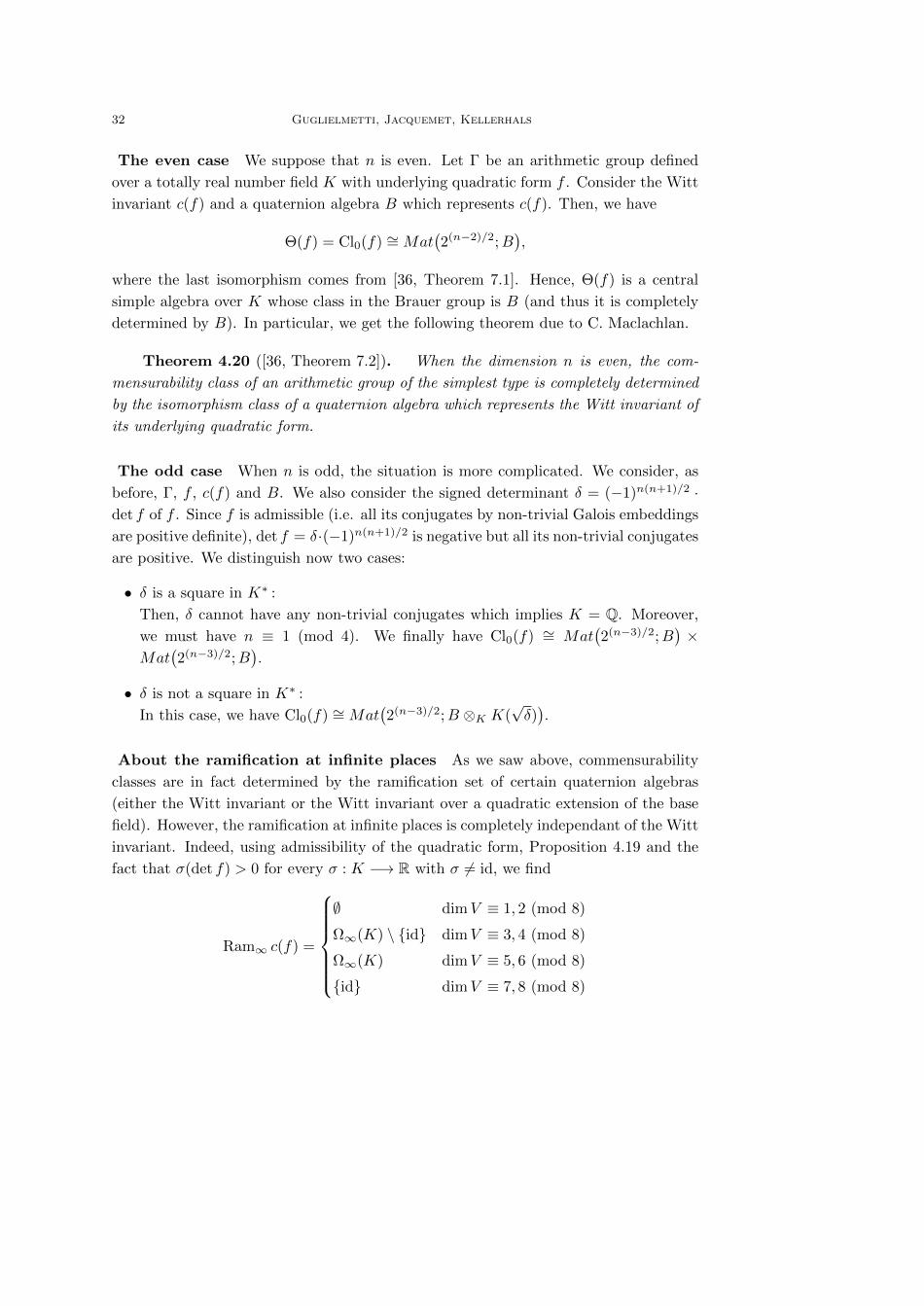
The odd case When n is odd, the situation is more complicated. We consider, as
before, Γ, f , c(f) and B. We also consider the signed determinant δ = (−1)n(n+1)/2 ·det f of f . Since f is admissible (i.e. all its conjugates by non-trivial Galois embeddings
are positive definite), det f = δ·(−1)n(n+1)/2 is negative but all its non-trivial conjugates
are positive. We distinguish now two cases:
• δ is a square in K∗ :
Then, δ cannot have any non-trivial conjugates which implies K = Q. Moreover,
we must have n ≡ 1 (mod 4). We finally have Cl0(f) ∼= Mat(2(n−3)/2;B
)×
Mat(2(n−3)/2;B
).
• δ is not a square in K∗ :
In this case, we have Cl0(f) ∼= Mat(2(n−3)/2;B ⊗K K(
√δ)).
About the ramification at infinite places As we saw above, commensurability
classes are in fact determined by the ramification set of certain quaternion algebras
(either the Witt invariant or the Witt invariant over a quadratic extension of the base
field). However, the ramification at infinite places is completely independant of the Witt
invariant. Indeed, using admissibility of the quadratic form, Proposition 4.19 and the
fact that σ(det f) > 0 for every σ : K −→ R with σ 6= id, we find
Ram∞ c(f) =
∅ dimV ≡ 1, 2 (mod 8)
Ω∞(K) \ id dimV ≡ 3, 4 (mod 8)
Ω∞(K) dimV ≡ 5, 6 (mod 8)
id dimV ≡ 7, 8 (mod 8)
Commensurability of hyperbolic Coxeter groups: theory and computation 33
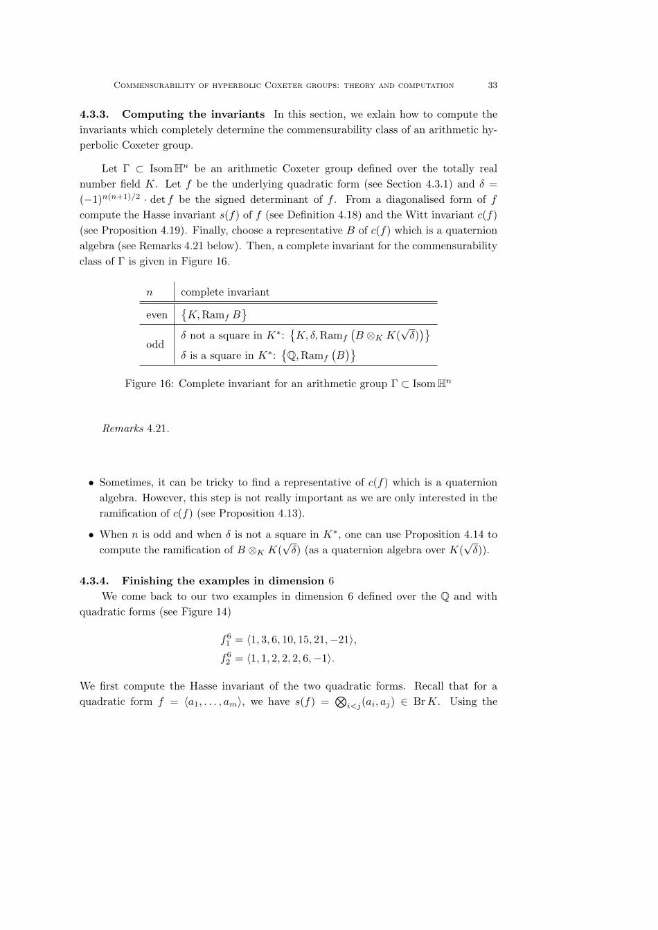
4.3.3. Computing the invariants In this section, we exlain how to compute the
invariants which completely determine the commensurability class of an arithmetic hy-
perbolic Coxeter group.
Let Γ ⊂ IsomHn be an arithmetic Coxeter group defined over the totally real
number field K. Let f be the underlying quadratic form (see Section 4.3.1) and δ =
(−1)n(n+1)/2 · det f be the signed determinant of f . From a diagonalised form of f
compute the Hasse invariant s(f) of f (see Definition 4.18) and the Witt invariant c(f)
(see Proposition 4.19). Finally, choose a representative B of c(f) which is a quaternion
algebra (see Remarks 4.21 below). Then, a complete invariant for the commensurability
class of Γ is given in Figure 16.
n complete invariant
evenK,Ramf B
odd
δ not a square in K∗:K, δ,Ramf
(B ⊗K K(
√δ))
δ is a square in K∗:Q,Ramf
(B)
Figure 16: Complete invariant for an arithmetic group Γ ⊂ IsomHn
Remarks 4.21.
• Sometimes, it can be tricky to find a representative of c(f) which is a quaternion
algebra. However, this step is not really important as we are only interested in the
ramification of c(f) (see Proposition 4.13).
• When n is odd and when δ is not a square in K∗, one can use Proposition 4.14 to
compute the ramification of B ⊗K K(√δ) (as a quaternion algebra over K(
√δ)).
4.3.4. Finishing the examples in dimension 6
We come back to our two examples in dimension 6 defined over the Q and with
quadratic forms (see Figure 14)
f61 = 〈1, 3, 6, 10, 15, 21,−21〉,f6
2 = 〈1, 1, 2, 2, 2, 6,−1〉.
We first compute the Hasse invariant of the two quadratic forms. Recall that for a
quadratic form f = 〈a1, . . . , am〉, we have s(f) =⊗
i<j(ai, aj) ∈ BrK. Using the
34 Guglielmetti, Jacquemet, Kellerhals
properties of Proposition 4.8, we compute:
s(f61 ) = (3, 6) · (3, 10) · (3, 15) ·
(3,−1)︷ ︸︸ ︷(3, 21) · (3,−21)
· (6, 10) · (6, 15) · (6,−1)
· (10, 15) · (10,−1)
· (15,−1)
= (5,−1).
Similarly, we find s(f62 ) = 1. By Proposition 4.19, we get c(f6
1 ) = (5,−1) · (−1,−3) =
(−1,−15) and c(f62 ) = 1 · (−1,−3). We find with Proposition 4.15 the followings
ramifications sets:
Ram(−1,−3) = 3,∞, Ram(−1, 5) = ∅.
Finally, Proposition 4.13 yields Ram c(f61 ) = 3,∞ = Ram c(f6
2 ), which implies that
the groups Γ61 and Γ6
2 are commensurable.
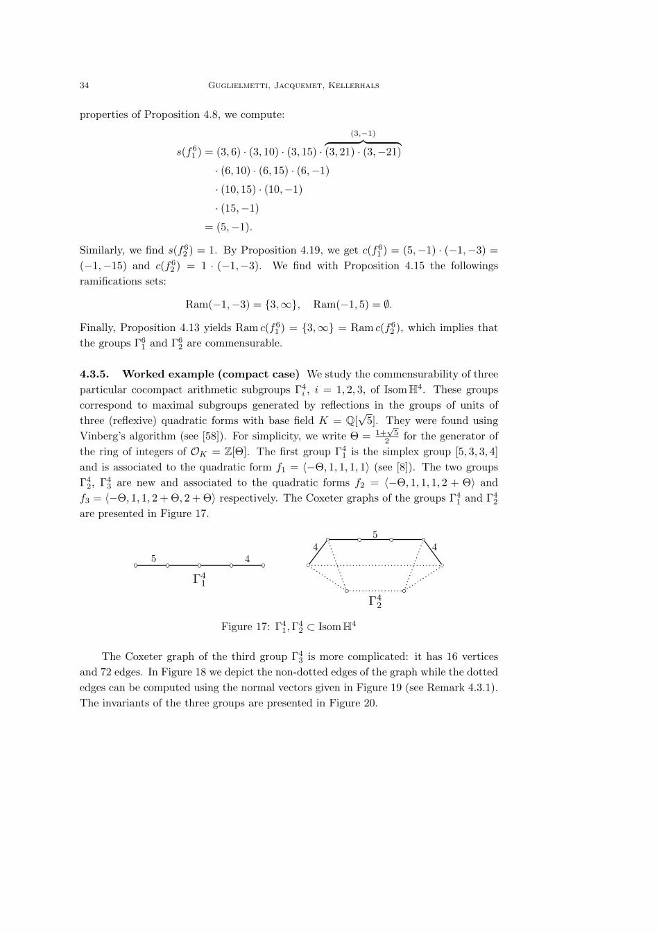
4.3.5. Worked example (compact case) We study the commensurability of three
particular cocompact arithmetic subgroups Γ4i , i = 1, 2, 3, of IsomH4. These groups
correspond to maximal subgroups generated by reflections in the groups of units of
three (reflexive) quadratic forms with base field K = Q[√
5]. They were found using
Vinberg’s algorithm (see [58]). For simplicity, we write Θ = 1+√
52 for the generator of
the ring of integers of OK = Z[Θ]. The first group Γ41 is the simplex group [5, 3, 3, 4]
and is associated to the quadratic form f1 = 〈−Θ, 1, 1, 1, 1〉 (see [8]). The two groups
Γ42, Γ4
3 are new and associated to the quadratic forms f2 = 〈−Θ, 1, 1, 1, 2 + Θ〉 and
f3 = 〈−Θ, 1, 1, 2 + Θ, 2 + Θ〉 respectively. The Coxeter graphs of the groups Γ41 and Γ4
2
are presented in Figure 17.
Figure 17: Γ41,Γ
42 ⊂ IsomH4
The Coxeter graph of the third group Γ43 is more complicated: it has 16 vertices
and 72 edges. In Figure 18 we depict the non-dotted edges of the graph while the dotted
edges can be computed using the normal vectors given in Figure 19 (see Remark 4.3.1).
The invariants of the three groups are presented in Figure 20.

Commensurability of hyperbolic Coxeter groups: theory and computation 35
Figure 18: Γ43 ⊂ IsomH4
e1 = (0,−1, 1, 0, 0), e4 = (0, 0, 0, 0,−1),
e2 = (0, 0,−1, 0, 0), e5 = (−1 + 1 ·Θ, 1 ·Θ, 0, 0, 0),
e3 = (0, 0, 0,−1, 1), e6 = (1, 0, 0, 1, 0),
e7 = (1 + 3 ·Θ, 2 + 1 ·Θ, 0, 1 + 1 ·Θ, 1 + 1 ·Θ),
e8 = (2 + 3 ·Θ, 1 + 2 ·Θ, 2 ·Θ, 1 + 1 ·Θ, 1 + 1 ·Θ),
e9 = (4 + 7 ·Θ, 3 + 4 ·Θ, 3 + 4 ·Θ, 2 + 3 ·Θ, 2 ·Θ),
e10 = (2 + 5 ·Θ, 1 + 2 ·Θ, 1 + 2 ·Θ, 1 + 2 ·Θ, 1 + 2 ·Θ),
e11 = (9 + 12 ·Θ, 4 + 7 ·Θ, 4 + 7 ·Θ, 3 + 6 ·Θ, 2 + 4 ·Θ),
e12 = (10 + 15 ·Θ, 4 + 7 ·Θ, 4 + 7 ·Θ, 4 + 7 ·Θ, 3 + 6 ·Θ),
e13 = (11 + 18 ·Θ, 7 + 11 ·Θ, 7 + 11 ·Θ, 4 + 7 ·Θ, 4 + 5 ·Θ),
e14 = (7 + 10 ·Θ, 4 + 6 ·Θ, 4 + 6 ·Θ, 3 + 4 ·Θ, 2 + 3 ·Θ),
e15 = (7 + 11 ·Θ, 4 + 7 ·Θ, 4 + 5 ·Θ, 3 + 5 ·Θ, 2 + 3 ·Θ),
e16 = (15 + 25 ·Θ, 10 + 15 ·Θ, 7 + 11 ·Θ, 7 + 11 ·Θ, 5 + 7 ·Θ).
Figure 19: Normal vectors for P (Γ43)
Since the dimension of the space is even, the commensurability class is completely
determined by the ramification set of the Witt invariant c(fi), i = 1, 2, 3, as indicated
in Theorem 4.20. Direct computations (see Figure 20) show that the Witt invariants
are given by
c(f1) = (−1,−1), c(f2) = (−Θ, 2 + Θ) · (−1,−1), c(f3) = (−1,−2−Θ).
Therefore, in order to decide about the commensurability of the groups, we have to
compute the finite ramification of the quaternion algebras (−1,−1)K , (−Θ, 2+Θ)K and
(−1, 2 + Θ)K . By Proposition 4.14, we get Ramf (−1,−1) = ∅. Since NK/Q(−Θ) = −1,
the element −Θ is invertible, and NK/Q(2 + Θ) = 5 implies that 2 + Θ is a prime
element of OK lying over 5. For a quaternion algebra (a, b)K , a necessary condition for
a prime ideal P ⊂ OK to belong to the ramification set is that P | 〈2ab〉 = (2ab)OK .
In our case, since 2 remains prime in OK , the only candidates are 2 and√
5. Moreover,
since the ramification set has even cardinality and since |Ram∞Bi| = 2, then either
Ramf Bi = ∅ or Ramf Bi = 2,√
5. To compute the ramification, we will use the
following theorem.
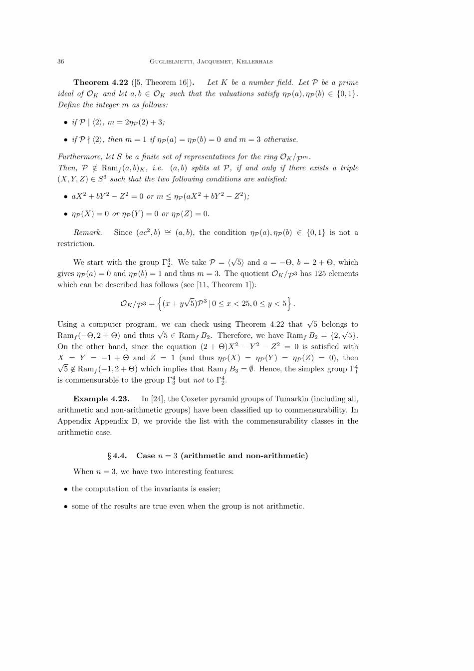
36 Guglielmetti, Jacquemet, Kellerhals
Theorem 4.22 ([5, Theorem 16]). Let K be a number field. Let P be a prime
ideal of OK and let a, b ∈ OK such that the valuations satisfy ηP(a), ηP(b) ∈ 0, 1.Define the integer m as follows:
• if P | 〈2〉, m = 2ηP(2) + 3;
• if P - 〈2〉, then m = 1 if ηP(a) = ηP(b) = 0 and m = 3 otherwise.
Furthermore, let S be a finite set of representatives for the ring OK/Pm.
Then, P /∈ Ramf (a, b)K , i.e. (a, b) splits at P, if and only if there exists a triple
(X,Y, Z) ∈ S3 such that the two following conditions are satisfied:
• aX2 + bY 2 − Z2 = 0 or m ≤ ηP(aX2 + bY 2 − Z2);
• ηP(X) = 0 or ηP(Y ) = 0 or ηP(Z) = 0.
Remark. Since (ac2, b) ∼= (a, b), the condition ηP(a), ηP(b) ∈ 0, 1 is not a
restriction.
We start with the group Γ42. We take P = 〈
√5〉 and a = −Θ, b = 2 + Θ, which
gives ηP(a) = 0 and ηP(b) = 1 and thus m = 3. The quotient OK/P3 has 125 elements
which can be described has follows (see [11, Theorem 1]):
OK/P3 =
(x+ y√
5)P3 | 0 ≤ x < 25, 0 ≤ y < 5.
Using a computer program, we can check using Theorem 4.22 that√
5 belongs to
Ramf (−Θ, 2 + Θ) and thus√
5 ∈ Ramf B2. Therefore, we have Ramf B2 = 2,√
5.On the other hand, since the equation (2 + Θ)X2 − Y 2 − Z2 = 0 is satisfied with
X = Y = −1 + Θ and Z = 1 (and thus ηP(X) = ηP(Y ) = ηP(Z) = 0), then√5 6∈ Ramf (−1, 2 + Θ) which implies that Ramf B3 = ∅. Hence, the simplex group Γ4
1
is commensurable to the group Γ43 but not to Γ4
2.
Example 4.23. In [24], the Coxeter pyramid groups of Tumarkin (including all,
arithmetic and non-arithmetic groups) have been classified up to commensurability. In
Appendix Appendix D, we provide the list with the commensurability classes in the
arithmetic case.
§ 4.4. Case n = 3 (arithmetic and non-arithmetic)
When n = 3, we have two interesting features:
• the computation of the invariants is easier;
• some of the results are true even when the group is not arithmetic.
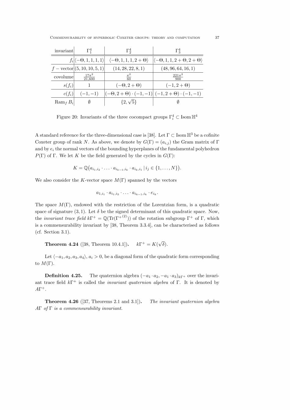
Commensurability of hyperbolic Coxeter groups: theory and computation 37
invariant Γ41 Γ4
2 Γ43
fi 〈−Θ, 1, 1, 1, 1〉 〈−Θ, 1, 1, 1, 2 + Θ〉 〈−Θ, 1, 1, 2 + Θ, 2 + Θ〉f − vector (5, 10, 10, 5, 1) (14, 28, 22, 8, 1) (48, 96, 64, 16, 1)
covolume 17π2
21,600π2
60221π2
900
s(fi) 1 (−Θ, 2 + Θ) (−1, 2 + Θ)
c(fi) (−1,−1) (−Θ, 2 + Θ) · (−1,−1) (−1, 2 + Θ) · (−1,−1)
Ramf Bi ∅ 2,√
5 ∅
Figure 20: Invariants of the three cocompact groups Γ4i ⊂ IsomH4
A standard reference for the three-dimensional case is [38]. Let Γ ⊂ IsomH3 be a cofinite
Coxeter group of rank N . As above, we denote by G(Γ) = (ai,j) the Gram matrix of Γ
and by ei the normal vectors of the bounding hyperplanes of the fundamental polyhedron
P (Γ) of Γ. We let K be the field generated by the cycles in G(Γ):
K = Q(ai1,i2 · . . . · aik−1,ik · aik,i1 | ij ∈ 1, . . . , N
).
We also consider the K-vector space M(Γ) spanned by the vectors
a1,i1 · ai1,i2 · . . . · aik−1,ik · eik .
The space M(Γ), endowed with the restriction of the Lorentzian form, is a quadratic
space of signature (3, 1). Let δ be the signed determinant of this quadratic space. Now,
the invariant trace field kΓ+ = Q(Tr(Γ+(2))) of the rotation subgroup Γ+ of Γ, which
is a commensurability invariant by [38, Theorem 3.3.4], can be characterised as follows
(cf. Section 3.1).
Theorem 4.24 ([38, Theorem 10.4.1]). kΓ+ = K(√δ).
Let 〈−a1, a2, a3, a4〉, ai > 0, be a diagonal form of the quadratic form corresponding
to M(Γ).
Definition 4.25. The quaternion algebra (−a1 ·a2,−a1 ·a3)kΓ+ over the invari-
ant trace field kΓ+ is called the invariant quaternion algebra of Γ. It is denoted by
AΓ+.
Theorem 4.26 ([37, Theorems 2.1 and 3.1]). The invariant quaternion algebra
AΓ of Γ is a commensurability invariant.
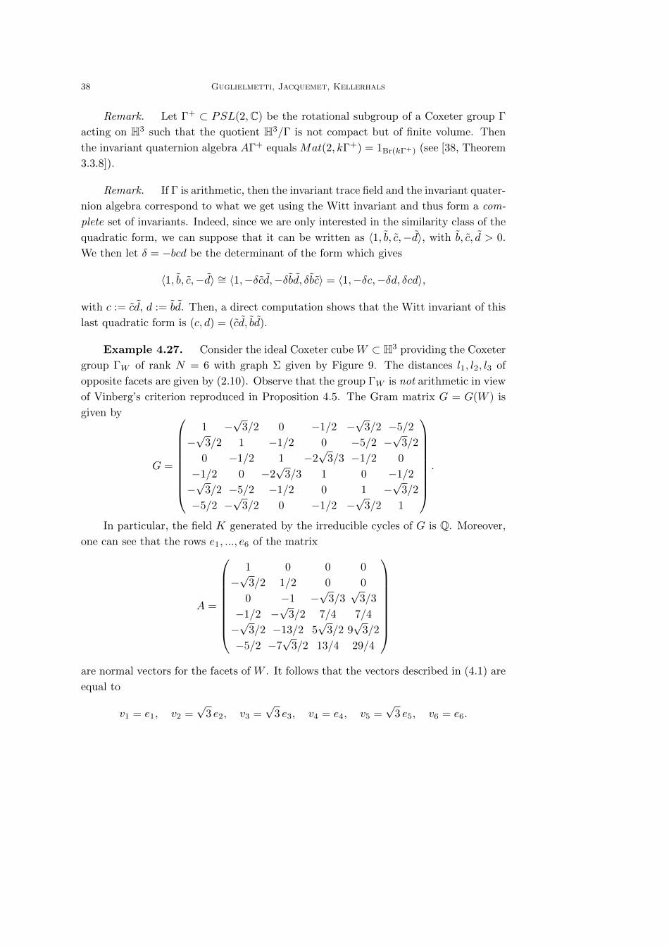
38 Guglielmetti, Jacquemet, Kellerhals
Remark. Let Γ+ ⊂ PSL(2,C) be the rotational subgroup of a Coxeter group Γ
acting on H3 such that the quotient H3/Γ is not compact but of finite volume. Then
the invariant quaternion algebra AΓ+ equals Mat(2, kΓ+) = 1Br(kΓ+) (see [38, Theorem
3.3.8]).
Remark. If Γ is arithmetic, then the invariant trace field and the invariant quater-
nion algebra correspond to what we get using the Witt invariant and thus form a com-
plete set of invariants. Indeed, since we are only interested in the similarity class of the
quadratic form, we can suppose that it can be written as 〈1, b, c,−d〉, with b, c, d > 0.
We then let δ = −bcd be the determinant of the form which gives
〈1, b, c,−d〉 ∼= 〈1,−δcd,−δbd, δbc〉 = 〈1,−δc,−δd, δcd〉,
with c := cd, d := bd. Then, a direct computation shows that the Witt invariant of this
last quadratic form is (c, d) = (cd, bd).
Example 4.27. Consider the ideal Coxeter cube W ⊂ H3 providing the Coxeter
group ΓW of rank N = 6 with graph Σ given by Figure 9. The distances l1, l2, l3 of
opposite facets are given by (2.10). Observe that the group ΓW is not arithmetic in view
of Vinberg’s criterion reproduced in Proposition 4.5. The Gram matrix G = G(W ) is
given by
G =
1 −√
3/2 0 −1/2 −√
3/2 −5/2
−√
3/2 1 −1/2 0 −5/2 −√
3/2
0 −1/2 1 −2√
3/3 −1/2 0
−1/2 0 −2√
3/3 1 0 −1/2
−√
3/2 −5/2 −1/2 0 1 −√
3/2
−5/2 −√
3/2 0 −1/2 −√
3/2 1
.
In particular, the field K generated by the irreducible cycles of G is Q. Moreover,
one can see that the rows e1, ..., e6 of the matrix
A =
1 0 0 0
−√
3/2 1/2 0 0
0 −1 −√
3/3√
3/3
−1/2 −√
3/2 7/4 7/4
−√
3/2 −13/2 5√
3/2 9√
3/2
−5/2 −7√
3/2 13/4 29/4
are normal vectors for the facets of W . It follows that the vectors described in (4.1) are
equal to
v1 = e1, v2 =√
3 e2, v3 =√
3 e3, v4 = e4, v5 =√
3 e5, v6 = e6.
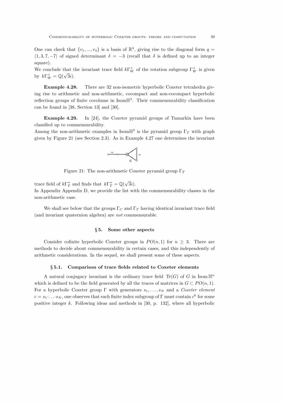
Commensurability of hyperbolic Coxeter groups: theory and computation 39
One can check that v1, ..., v4 is a basis of R4, giving rise to the diagonal form q =
〈1, 3, 7,−7〉 of signed determinant δ = −3 (recall that δ is defined up to an integer
square).
We conclude that the invariant trace field kΓ+W of the rotation subgroup Γ+
W is given
by kΓ+W = Q(
√3i).
Example 4.28. There are 32 non-isometric hyperbolic Coxeter tetrahedra giv-
ing rise to arithmetic and non-arithmetic, cocompact and non-cocompact hyperbolic
reflection groups of finite covolume in IsomH3. Their commensurability classification
can be found in [38, Section 13] and [30].
Example 4.29. In [24], the Coxeter pyramid groups of Tumarkin have been
classified up to commensurability.
Among the non-arithmetic examples in IsomH3 is the pyramid group ΓT with graph
given by Figure 21 (see Section 2.3). As in Example 4.27 one determines the invariant
b b be bbQQ
∞∞
6
Figure 21: The non-arithmetic Coxeter pyramid group ΓT
trace field of kΓ+T and finds that kΓ+
T = Q(√
3i).
In Appendix Appendix D, we provide the list with the commensurability classes in the
non-arithmetic case.
We shall see below that the groups ΓC and ΓT having identical invariant trace field
(and invariant quaternion algebra) are not commensurable.
§ 5. Some other aspects
Consider cofinite hyperbolic Coxeter groups in PO(n, 1) for n ≥ 3. There are
methods to decide about commensurability in certain cases, and this independently of
arithmetic considerations. In the sequel, we shall present some of these aspects.
§ 5.1. Comparison of trace fields related to Coxeter elements
A natural conjugacy invariant is the ordinary trace field Tr(G) of G in IsomHn
which is defined to be the field generated by all the traces of matrices in G ⊂ PO(n, 1).
For a hyperbolic Coxeter group Γ with generators s1, . . . , sN and a Coxeter element
c = s1·. . .·sN , one observes that each finite index subgroup of Γ must contain ck for some
positive integer k. Following ideas and methods in [30, p. 132], where all hyperbolic
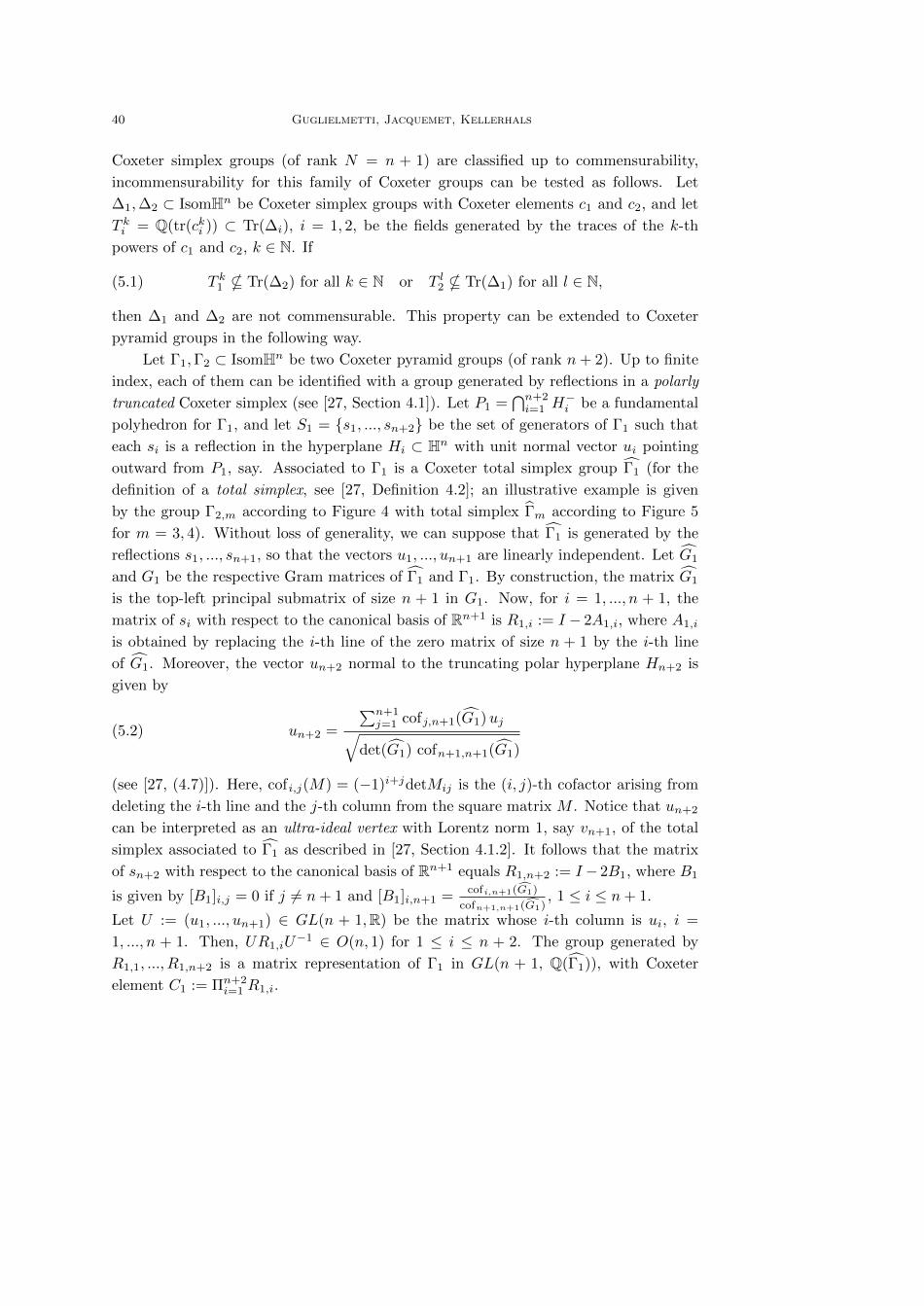
40 Guglielmetti, Jacquemet, Kellerhals
Coxeter simplex groups (of rank N = n + 1) are classified up to commensurability,
incommensurability for this family of Coxeter groups can be tested as follows. Let
∆1,∆2 ⊂ IsomHn be Coxeter simplex groups with Coxeter elements c1 and c2, and let
T ki = Q(tr(cki )) ⊂ Tr(∆i), i = 1, 2, be the fields generated by the traces of the k-th
powers of c1 and c2, k ∈ N. If
(5.1) T k1 * Tr(∆2) for all k ∈ N or T l2 * Tr(∆1) for all l ∈ N,
then ∆1 and ∆2 are not commensurable. This property can be extended to Coxeter
pyramid groups in the following way.
Let Γ1,Γ2 ⊂ IsomHn be two Coxeter pyramid groups (of rank n+ 2). Up to finite
index, each of them can be identified with a group generated by reflections in a polarly
truncated Coxeter simplex (see [27, Section 4.1]). Let P1 =⋂n+2i=1 H
−i be a fundamental
polyhedron for Γ1, and let S1 = s1, ..., sn+2 be the set of generators of Γ1 such that
each si is a reflection in the hyperplane Hi ⊂ Hn with unit normal vector ui pointing
outward from P1, say. Associated to Γ1 is a Coxeter total simplex group Γ1 (for the
definition of a total simplex, see [27, Definition 4.2]; an illustrative example is given
by the group Γ2,m according to Figure 4 with total simplex Γm according to Figure 5
for m = 3, 4). Without loss of generality, we can suppose that Γ1 is generated by the
reflections s1, ..., sn+1, so that the vectors u1, ..., un+1 are linearly independent. Let G1
and G1 be the respective Gram matrices of Γ1 and Γ1. By construction, the matrix G1
is the top-left principal submatrix of size n + 1 in G1. Now, for i = 1, ..., n + 1, the
matrix of si with respect to the canonical basis of Rn+1 is R1,i := I − 2A1,i, where A1,i
is obtained by replacing the i-th line of the zero matrix of size n + 1 by the i-th line
of G1. Moreover, the vector un+2 normal to the truncating polar hyperplane Hn+2 is
given by
(5.2) un+2 =
∑n+1j=1 cofj,n+1(G1)uj√
det(G1) cofn+1,n+1(G1)
(see [27, (4.7)]). Here, cofi,j(M) = (−1)i+jdetMij is the (i, j)-th cofactor arising from
deleting the i-th line and the j-th column from the square matrix M . Notice that un+2
can be interpreted as an ultra-ideal vertex with Lorentz norm 1, say vn+1, of the total
simplex associated to Γ1 as described in [27, Section 4.1.2]. It follows that the matrix
of sn+2 with respect to the canonical basis of Rn+1 equals R1,n+2 := I − 2B1, where B1
is given by [B1]i,j = 0 if j 6= n+ 1 and [B1]i,n+1 =cofi,n+1(G1)
cofn+1,n+1(G1), 1 ≤ i ≤ n+ 1.
Let U := (u1, ..., un+1) ∈ GL(n + 1,R) be the matrix whose i-th column is ui, i =
1, ..., n + 1. Then, UR1,iU−1 ∈ O(n, 1) for 1 ≤ i ≤ n + 2. The group generated by
R1,1, ..., R1,n+2 is a matrix representation of Γ1 in GL(n + 1, Q(Γ1)), with Coxeter
element C1 := Πn+2i=1 R1,i.
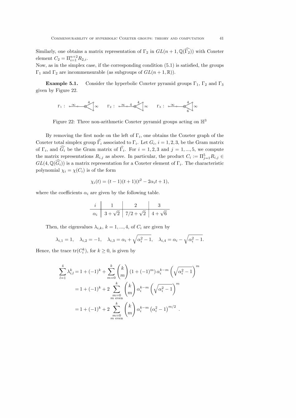
Commensurability of hyperbolic Coxeter groups: theory and computation 41
Similarly, one obtains a matrix representation of Γ2 in GL(n+ 1,Q(Γ2)) with Coxeter
element C2 = Πn+2i=1 R2,i.
Now, as in the simplex case, if the corresponding condition (5.1) is satisfied, the groups
Γ1 and Γ2 are incommensurable (as subgroups of GL(n+ 1,R)).
Example 5.1. Consider the hyperbolic Coxeter pyramid groups Γ1, Γ2 and Γ3
given by Figure 22.
a a ad aaHH4
Γ1 : ∞ ∞ a a ad aaHH4
4Γ2 : ∞ ∞ a a ad aaHH4
6
Γ3 : ∞ ∞
Figure 22: Three non-arithmetic Coxeter pyramid groups acting on H3
By removing the first node on the left of Γi, one obtains the Coxeter graph of the
Coxeter total simplex group Γi associated to Γi. Let Gi, i = 1, 2, 3, be the Gram matrix
of Γi, and Gi be the Gram matrix of Γi. For i = 1, 2, 3 and j = 1, ..., 5, we compute
the matrix representations Ri,j as above. In particular, the product Ci := Π5j=1Ri,j ∈
GL(4,Q(Gi)) is a matrix representation for a Coxeter element of Γi. The characteristic
polynomial χi = χ(Ci) is of the form
χi(t) = (t− 1)(t+ 1)(t2 − 2αit+ 1),
where the coefficients αi are given by the following table.
i 1 2 3
αi 3 +√
2 7/2 +√
2 4 +√
6
Then, the eigenvalues λi,k, k = 1, ..., 4, of Ci are given by
λi,1 = 1, λi,2 = −1, λi,3 = αi +√α2i − 1, λi,4 = αi −
√α2i − 1.
Hence, the trace tr(Cki ), for k ≥ 0, is given by
4∑l=1
λki,l = 1 + (−1)k +k∑
m=0
(k
m
)(1 + (−1)m)αk−mi
(√α2i − 1
)m
= 1 + (−1)k + 2k∑
m=0m even
(k
m
)αk−mi
(√α2i − 1
)m
= 1 + (−1)k + 2
k∑m=0m even
(k
m
)αk−mi
(α2i − 1
)m/2.
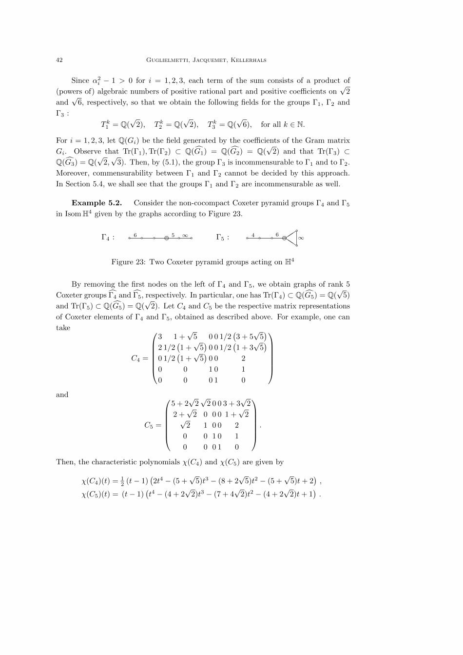
42 Guglielmetti, Jacquemet, Kellerhals
Since α2i − 1 > 0 for i = 1, 2, 3, each term of the sum consists of a product of
(powers of) algebraic numbers of positive rational part and positive coefficients on√
2
and√
6, respectively, so that we obtain the following fields for the groups Γ1, Γ2 and
Γ3 :
T k1 = Q(√
2), T k2 = Q(√
2), T k3 = Q(√
6), for all k ∈ N.
For i = 1, 2, 3, let Q(Gi) be the field generated by the coefficients of the Gram matrix
Gi. Observe that Tr(Γ1),Tr(Γ2) ⊂ Q(G1) = Q(G2) = Q(√
2) and that Tr(Γ3) ⊂Q(G3) = Q(
√2,√
3). Then, by (5.1), the group Γ3 is incommensurable to Γ1 and to Γ2.
Moreover, commensurability between Γ1 and Γ2 cannot be decided by this approach.
In Section 5.4, we shall see that the groups Γ1 and Γ2 are incommensurable as well.
Example 5.2. Consider the non-cocompact Coxeter pyramid groups Γ4 and Γ5
in IsomH4 given by the graphs according to Figure 23.
da a a a a a6 5 ∞Γ4 : daaaa aaQQ
64 ∞Γ5 :
Figure 23: Two Coxeter pyramid groups acting on H4
By removing the first nodes on the left of Γ4 and Γ5, we obtain graphs of rank 5
Coxeter groups Γ4 and Γ5, respectively. In particular, one has Tr(Γ4) ⊂ Q(G5) = Q(√
5)
and Tr(Γ5) ⊂ Q(G5) = Q(√
2). Let C4 and C5 be the respective matrix representations
of Coxeter elements of Γ4 and Γ5, obtained as described above. For example, one can
take
C4 =
3 1 +
√5 0 0 1/2
(3 + 5
√5)
2 1/2(1 +√
5)
0 0 1/2(1 + 3
√5)
0 1/2(1 +√
5)
0 0 2
0 0 1 0 1
0 0 0 1 0
and
C5 =
5 + 2
√2√
2 0 0 3 + 3√
2
2 +√
2 0 0 0 1 +√
2√2 1 0 0 2
0 0 1 0 1
0 0 0 1 0
.
Then, the characteristic polynomials χ(C4) and χ(C5) are given by
χ(C4)(t) = 12 (t− 1)
(2t4 − (5 +
√5)t3 − (8 + 2
√5)t2 − (5 +
√5)t+ 2
),
χ(C5)(t) = (t− 1)(t4 − (4 + 2
√2)t3 − (7 + 4
√2)t2 − (4 + 2
√2)t+ 1
).
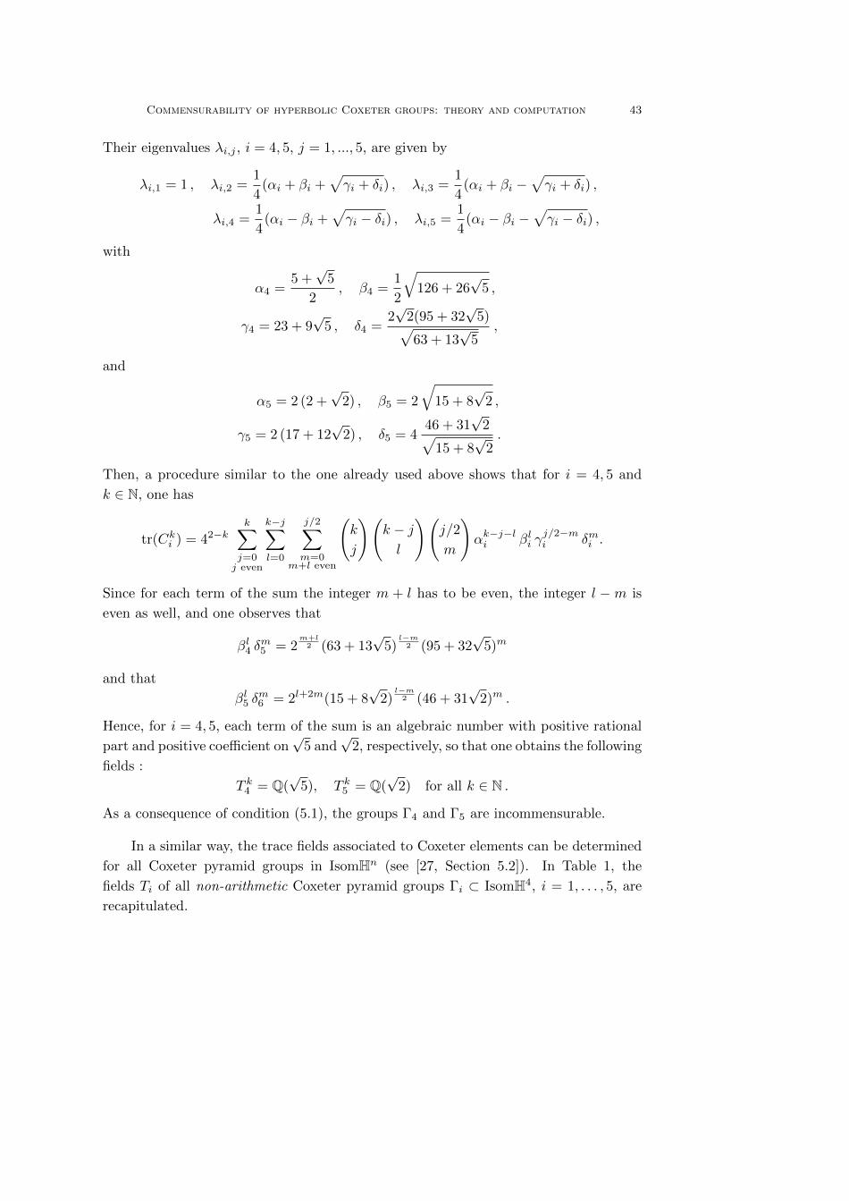
Commensurability of hyperbolic Coxeter groups: theory and computation 43
Their eigenvalues λi,j , i = 4, 5, j = 1, ..., 5, are given by
λi,1 = 1 , λi,2 =1
4(αi + βi +
√γi + δi) , λi,3 =
1
4(αi + βi −
√γi + δi) ,
λi,4 =1
4(αi − βi +
√γi − δi) , λi,5 =
1
4(αi − βi −
√γi − δi) ,
with
α4 =5 +√
5
2, β4 =
1
2
√126 + 26
√5 ,
γ4 = 23 + 9√
5 , δ4 =2√
2(95 + 32√
5)√63 + 13
√5
,
and
α5 = 2 (2 +√
2) , β5 = 2
√15 + 8
√2 ,
γ5 = 2 (17 + 12√
2) , δ5 = 446 + 31
√2√
15 + 8√
2.
Then, a procedure similar to the one already used above shows that for i = 4, 5 and
k ∈ N, one has
tr(Cki ) = 42−kk∑j=0j even
k−j∑l=0
j/2∑m=0
m+l even
(k
j
)(k − jl
)(j/2
m
)αk−j−li βli γ
j/2−mi δmi .
Since for each term of the sum the integer m + l has to be even, the integer l −m is
even as well, and one observes that
βl4 δm5 = 2
m+l2 (63 + 13
√5)
l−m2 (95 + 32
√5)m
and that
βl5 δm6 = 2l+2m(15 + 8
√2)
l−m2 (46 + 31
√2)m .
Hence, for i = 4, 5, each term of the sum is an algebraic number with positive rational
part and positive coefficient on√
5 and√
2, respectively, so that one obtains the following
fields :
T k4 = Q(√
5), T k5 = Q(√
2) for all k ∈ N .
As a consequence of condition (5.1), the groups Γ4 and Γ5 are incommensurable.
In a similar way, the trace fields associated to Coxeter elements can be determined
for all Coxeter pyramid groups in IsomHn (see [27, Section 5.2]). In Table 1, the
fields Ti of all non-arithmetic Coxeter pyramid groups Γi ⊂ IsomH4, i = 1, . . . , 5, are
recapitulated.
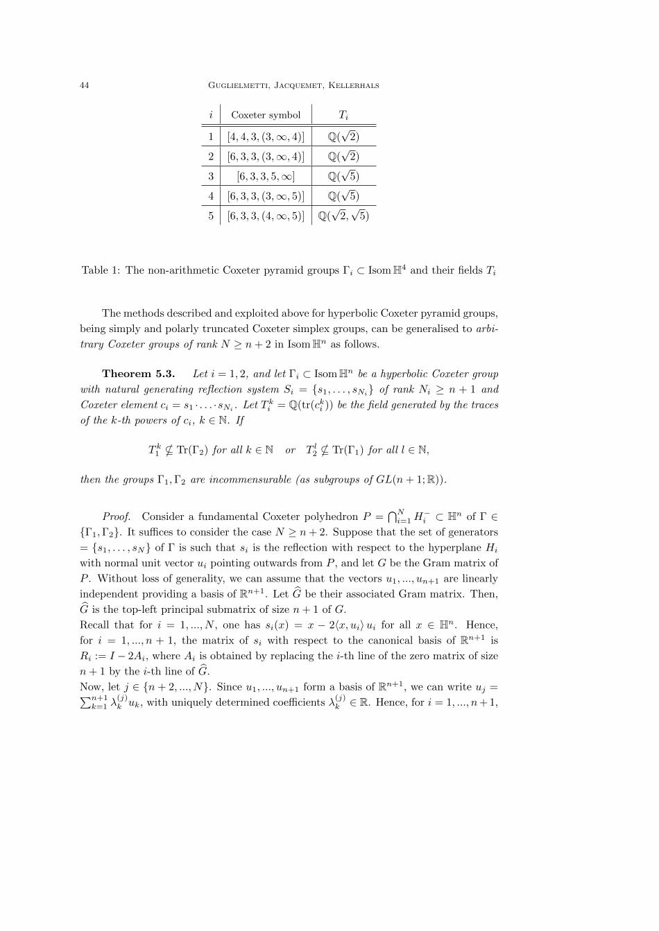
44 Guglielmetti, Jacquemet, Kellerhals
i Coxeter symbol Ti
1 [4, 4, 3, (3,∞, 4)] Q(√
2)
2 [6, 3, 3, (3,∞, 4)] Q(√
2)
3 [6, 3, 3, 5,∞] Q(√
5)
4 [6, 3, 3, (3,∞, 5)] Q(√
5)
5 [6, 3, 3, (4,∞, 5)] Q(√
2,√
5)
Table 1: The non-arithmetic Coxeter pyramid groups Γi ⊂ IsomH4 and their fields Ti
The methods described and exploited above for hyperbolic Coxeter pyramid groups,
being simply and polarly truncated Coxeter simplex groups, can be generalised to arbi-
trary Coxeter groups of rank N ≥ n+ 2 in IsomHn as follows.
Theorem 5.3. Let i = 1, 2, and let Γi ⊂ IsomHn be a hyperbolic Coxeter group
with natural generating reflection system Si = s1, . . . , sNi of rank Ni ≥ n + 1 and
Coxeter element ci = s1 · . . . ·sNi . Let T ki = Q(tr(cki )) be the field generated by the traces
of the k-th powers of ci, k ∈ N. If
T k1 * Tr(Γ2) for all k ∈ N or T l2 * Tr(Γ1) for all l ∈ N,
then the groups Γ1,Γ2 are incommensurable (as subgroups of GL(n+ 1;R)).
Proof. Consider a fundamental Coxeter polyhedron P =⋂Ni=1H
−i ⊂ Hn of Γ ∈
Γ1,Γ2. It suffices to consider the case N ≥ n+ 2. Suppose that the set of generators
= s1, . . . , sN of Γ is such that si is the reflection with respect to the hyperplane Hi
with normal unit vector ui pointing outwards from P , and let G be the Gram matrix of
P . Without loss of generality, we can assume that the vectors u1, ..., un+1 are linearly
independent providing a basis of Rn+1. Let G be their associated Gram matrix. Then,
G is the top-left principal submatrix of size n+ 1 of G.
Recall that for i = 1, ..., N , one has si(x) = x − 2〈x, ui〉ui for all x ∈ Hn. Hence,
for i = 1, ..., n + 1, the matrix of si with respect to the canonical basis of Rn+1 is
Ri := I − 2Ai, where Ai is obtained by replacing the i-th line of the zero matrix of size
n+ 1 by the i-th line of G.
Now, let j ∈ n+ 2, ..., N. Since u1, ..., un+1 form a basis of Rn+1, we can write uj =∑n+1k=1 λ
(j)k uk, with uniquely determined coefficients λ
(j)k ∈ R. Hence, for i = 1, ..., n+ 1,
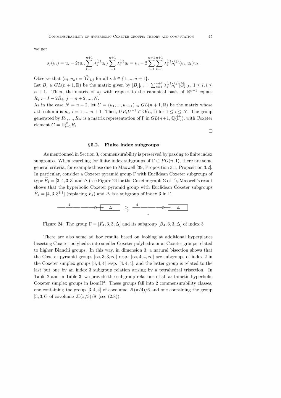
Commensurability of hyperbolic Coxeter groups: theory and computation 45
we get
sj(ui) = ui − 2〈ui,n+1∑k=1
λ(j)k uk〉
n+1∑l=1
λ(j)l ul = ui − 2
n+1∑l=1
n+1∑k=1
λ(j)k λ
(j)l 〈ui, uk〉ul.
Observe that 〈ui, uk〉 = [G]i,j for all i, k ∈ 1, ..., n+ 1.Let Bj ∈ GL(n + 1,R) be the matrix given by [Bj ]l,i =
∑n+1k=1 λ
(j)k λ
(j)l [G]i,k, 1 ≤ l, i ≤
n + 1. Then, the matrix of sj with respect to the canonical basis of Rn+1 equals
Rj := I − 2Bj , j = n+ 2, ..., N .
As in the case N = n + 2, let U = (u1, ..., un+1) ∈ GL(n + 1,R) be the matrix whose
i-th column is ui, i = 1, ..., n + 1. Then, URiU−1 ∈ O(n, 1) for 1 ≤ i ≤ N . The group
generated by R1, ..., RN is a matrix representation of Γ in GL(n+1, Q(Γ)), with Coxeter
element C = ΠNi=1Ri.
§ 5.2. Finite index subgroups
As mentionned in Section 3, commensurability is preserved by passing to finite index
subgroups. When searching for finite index subgroups of Γ ⊂ PO(n, 1), there are some
general criteria, for example those due to Maxwell [39, Proposition 3.1, Proposition 3.2].
In particular, consider a Coxeter pyramid group Γ with Euclidean Coxeter subgroups of
type F4 = [3, 4, 3, 3] and ∆ (see Figure 24 for the Coxeter graph Σ of Γ), Maxwell’s result
shows that the hyperbolic Coxeter pyramid group with Euclidean Coxeter subgroups
B4 = [4, 3, 31,1] (replacing F4) and ∆ is a subgroup of index 3 in Γ.
a a a a a ad a4∆ a a aa a ad a4
∆>3
Figure 24: The group Γ = [F4, 3, 3,∆] and its subgroup [B4, 3, 3,∆] of index 3
There are also some ad hoc results based on looking at additional hyperplanes
bisecting Coxeter polyhedra into smaller Coxeter polyhedra or at Coxeter groups related
to higher Bianchi groups. In this way, in dimension 3, a natural bisection shows that
the Coxeter pyramid groups [∞, 3, 3,∞] resp. [∞, 4, 4,∞] are subgroups of index 2 in
the Coxeter simplex groups [3, 4, 4] resp. [4, 4, 4], and the latter group is related to the
last but one by an index 3 subgroup relation arising by a tetrahedral trisection. In
Table 2 and in Table 3, we provide the subgroup relations of all arithmetic hyperbolic
Coxeter simplex groups in IsomH3. These groups fall into 2 commensurability classes,
one containing the group [3, 4, 4] of covolume L(π/4)/6 and one containing the group
[3, 3, 6] of covolume L(π/3)/8 (see (2.8)).
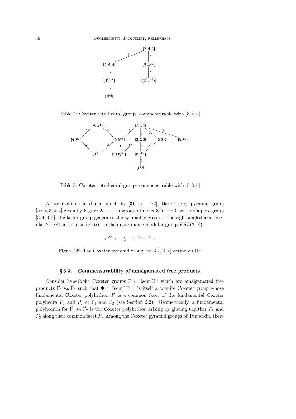
46 Guglielmetti, Jacquemet, Kellerhals
[3,4,4]
[3,41,1]
[(32,42)]
[4,4,4]
[41,1,1]
[4[4]]
.......................................................................................................................................................................................
3
..................................................................
2
..................................................................
2
..................................................................
2
..................................................................
2
Table 2: Coxeter tetrahedral groups commensurable with [3, 4, 4]
[3,3,6]
[3,3[3]]
[4,3,6]
[4,3[3]] [6,31,1] [3,6,3] [6,3,6]
[(3,6)[2]] [6,3[3]][3[]×[ ]
[3[3,3]]
................................................................................................
5................................................................................................
2................................................................................................
2..................................................................4
........................................................................................................6
............................................................................................................................................................................................................................
2
................................................................................................
2................................................................................................
2..................................................................
4
................................................................................................
5..................................................................
3
................................................................................................
2
..................................................................
2
Table 3: Coxeter tetrahedral groups commensurable with [3, 3, 6]
As an example in dimension 4, by [31, p. 172], the Coxeter pyramid group
[∞, 3, 3, 4, 4] given by Figure 25 is a subgroup of index 3 in the Coxeter simplex group
[3, 4, 3, 4]; the latter group generates the symmetry group of the right-angled ideal reg-
ular 24-cell and is also related to the quaternionic modular group PSL(2,H).
b b be b b b∞ 4 4
Figure 25: The Coxeter pyramid group [∞, 3, 3, 4, 4] acting on H4
§ 5.3. Commensurability of amalgamated free products
Consider hyperbolic Coxeter groups Γ ⊂ IsomHn which are amalgamated free
products Γ1 ?Φ Γ2 such that Φ ⊂ IsomHn−1 is itself a cofinite Coxeter group whose
fundamental Coxeter polyhedron F is a common facet of the fundamental Coxeter
polyhedra P1 and P2 of Γ1 and Γ2 (see Section 2.2). Geometrically, a fundamental
polyhedron for Γ1 ?Φ Γ2 is the Coxeter polyhedron arising by glueing together P1 and
P2 along their common facet F . Among the Coxeter pyramid groups of Tumarkin, there
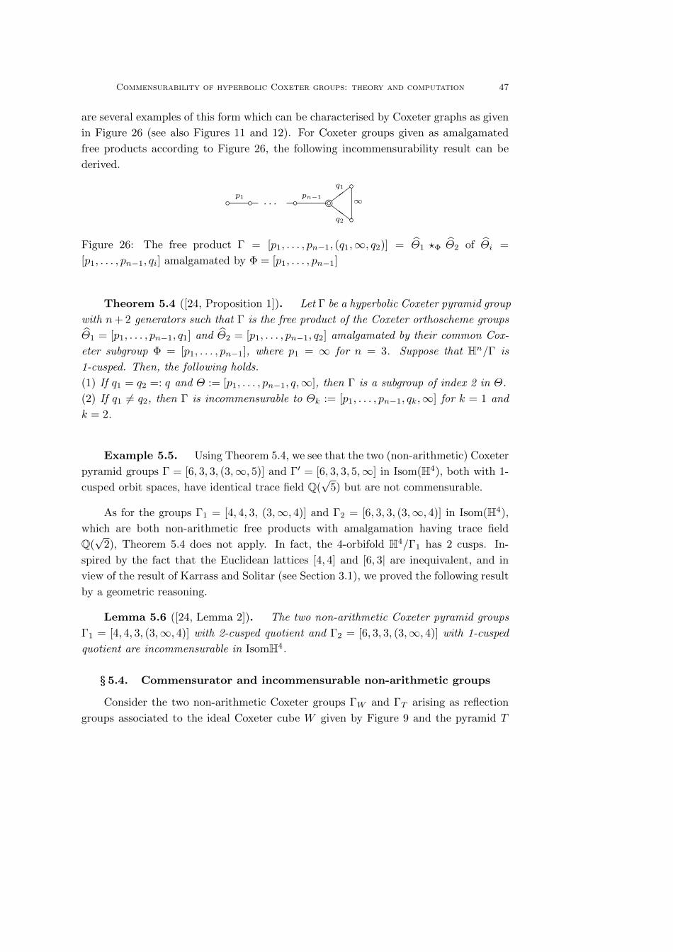
Commensurability of hyperbolic Coxeter groups: theory and computation 47
are several examples of this form which can be characterised by Coxeter graphs as given
in Figure 26 (see also Figures 11 and 12). For Coxeter groups given as amalgamated
free products according to Figure 26, the following incommensurability result can be
derived.
b b b be bb
ZZ
p1 pn−1
q1
q2
∞. . .
Figure 26: The free product Γ = [p1, . . . , pn−1, (q1,∞, q2)] = Θ1 ?Φ Θ2 of Θi =
[p1, . . . , pn−1, qi] amalgamated by Φ = [p1, . . . , pn−1]
Theorem 5.4 ([24, Proposition 1]). Let Γ be a hyperbolic Coxeter pyramid group
with n+ 2 generators such that Γ is the free product of the Coxeter orthoscheme groups
Θ1 = [p1, . . . , pn−1, q1] and Θ2 = [p1, . . . , pn−1, q2] amalgamated by their common Cox-
eter subgroup Φ = [p1, . . . , pn−1], where p1 = ∞ for n = 3. Suppose that Hn/Γ is
1-cusped. Then, the following holds.
(1) If q1 = q2 =: q and Θ := [p1, . . . , pn−1, q,∞], then Γ is a subgroup of index 2 in Θ.
(2) If q1 6= q2, then Γ is incommensurable to Θk := [p1, . . . , pn−1, qk,∞] for k = 1 and
k = 2.
Example 5.5. Using Theorem 5.4, we see that the two (non-arithmetic) Coxeter
pyramid groups Γ = [6, 3, 3, (3,∞, 5)] and Γ′ = [6, 3, 3, 5,∞] in Isom(H4), both with 1-
cusped orbit spaces, have identical trace field Q(√
5) but are not commensurable.
As for the groups Γ1 = [4, 4, 3, (3,∞, 4)] and Γ2 = [6, 3, 3, (3,∞, 4)] in Isom(H4),
which are both non-arithmetic free products with amalgamation having trace field
Q(√
2), Theorem 5.4 does not apply. In fact, the 4-orbifold H4/Γ1 has 2 cusps. In-
spired by the fact that the Euclidean lattices [4, 4] and [6, 3| are inequivalent, and in
view of the result of Karrass and Solitar (see Section 3.1), we proved the following result
by a geometric reasoning.
Lemma 5.6 ([24, Lemma 2]). The two non-arithmetic Coxeter pyramid groups
Γ1 = [4, 4, 3, (3,∞, 4)] with 2-cusped quotient and Γ2 = [6, 3, 3, (3,∞, 4)] with 1-cusped
quotient are incommensurable in IsomH4.
§ 5.4. Commensurator and incommensurable non-arithmetic groups
Consider the two non-arithmetic Coxeter groups ΓW and ΓT arising as reflection
groups associated to the ideal Coxeter cube W given by Figure 9 and the pyramid T
48 Guglielmetti, Jacquemet, Kellerhals
given by Figure 12 in H3. Their rotation subgroups have identical invariant trace field
and invariant quaternion algebra, respectively. By having a look at the covolume ratio
based on the values (2.11) and (2.14), an accurate numerical check indicates that the
quotient
ω : =covol3(ΓT )
covol3(ΓW )=
54 L(π3 ) + 1
3 L(π4 )
10 L(π3 )=
1
8+
1
30
L(π4 )
L(π3 )
∼ 0.1701240538565287
(5.3)
is an irrational number implying the incommensurability of the groups ΓT and ΓW .
Let us prove rigorously that ω defined by (5.3) is irrational. We assume the contrary
and suppose that ΓT and ΓW are commensurable. Let C denote their commensurator
(see Section 3.1). Since ΓT and ΓW are non-arithmetic, by Margulis’ Theorem 3.1, the
group C is a discrete subgroup of IsomH3 containing both groups as subgroups of finite
indices. Furthermore, C is a non-cocompact but cofinite (non-arithmetic) group so that
its covolume is universally bounded from below by the minimal covolume L(π/3)/8 in
this class which is realised by the tetrahedral group [3, 3, 6] (see [42] and [34, Table 2]).
This allows us to rewrite (5.3) according to
(5.4) ω =covol3(ΓT )
covol3(ΓW )=
covol3(ΓT )/covol3(C)
covol3(ΓW )/covol3(C)=
[C : ΓT ]
[C : ΓW ].
Now, since covol3(ΓW ) = 10 L(π/3) and covol3([3, 3, 6]) = 18 L(π/3) , we get that
[C : ΓW ] < 80. Using this and (5.4), it is easy to check that there is no rational
solution ω to (5.3) with an approximate value ω ∼ 0.1701240538565287. This provides
the desired contradiction. A similar reasoning based on the covolume expressions (2.13)
allows us to prove that the two non-arithmetic Coxeter pyramid groups [∞, 3, (3,∞, 4)]
with 1-cusped quotient and [∞, 3, (4,∞, 4)] with 2-cusped quotient, both groups having
identical invariant trace field and invariant quaternion algebra, are incommensurable in
IsomH3. In this way, the commensurability classification for the family of Tumarkin’s
Coxeter pyramid groups could be finalised. In Appendix Appendix D, we provide the
commensurability classes of all non-arithmetic Coxeter pyramid groups.
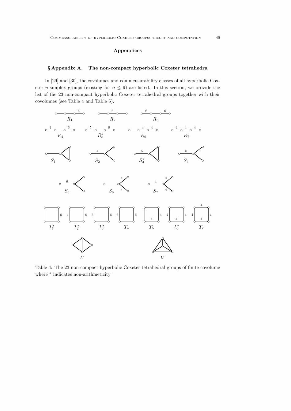
Commensurability of hyperbolic Coxeter groups: theory and computation 49
Appendices
§Appendix A. The non-compact hyperbolic Coxeter tetrahedra
In [29] and [30], the covolumes and commensurability classes of all hyperbolic Cox-
eter n-simplex groups (existing for n ≤ 9) are listed. In this section, we provide the
list of the 23 non-compact hyperbolic Coxeter tetrahedral groups together with their
covolumes (see Table 4 and Table 5).
R1 R2 R3
6 6 6 6
R4
4 6
R∗5
5 6
R6
4 4
R7
4 4 4
...........................................................................................................
...........................................................................................................
...........................................................................................................
...........................................................................................................
S1 S2 S∗3 S4
4 5 6
S5 S6 S7
64
4
44
4
T ∗1 T ∗
2 T ∗3 T4 T5 T ∗
6 T7
6 6 6 6 4 4 44 5 64 4 4
44
4
4
U V
..........................................................................................................
..........................................................................................................
..........................................................................................................
.............................................................................................................................................................................................................................................................
...................................................
........................................................................
..............................
.....................................................
Table 4: The 23 non-compact hyperbolic Coxeter tetrahedral groups of finite covolume
where ∗ indicates non-arithmeticity
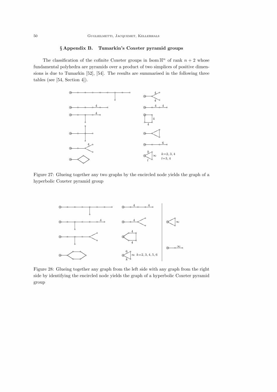
50 Guglielmetti, Jacquemet, Kellerhals
§Appendix B. Tumarkin’s Coxeter pyramid groups
The classification of the cofinite Coxeter groups in IsomHn of rank n + 2 whose
fundamental polyhedra are pyramids over a product of two simplices of positive dimen-
sions is due to Tumarkin [52], [54]. The results are summarised in the following three
tables (see [54, Section 4]).
da a aa aQQQQ
ad a a aaHH4
ad a a aaa
ad a aa a a4
ad a a a a a4
ad a a a a a aa a a ad a aaHH4
4ad a a a4 4ad aa a4
4
ad a aaHH
6ad a a aad aaHHk
l
k=2, 3, 4
l=3, 4∞
Figure 27: Glueing together any two graphs by the encircled node yields the graph of a
hyperbolic Coxeter pyramid group
da a aa aa aQQ
da a aa a a aaHH
da a aa a a a a4
da a a aa a a a a da a a a a4 4
da a a aaHH
4
da aa aaQQ
4
4
da aaHH6
k
k=2, 3, 4, 5, 6∞
da aaHH
∞
da a a∞
Figure 28: Glueing together any graph from the left side with any graph from the right
side by identifying the encircled node yields the graph of a hyperbolic Coxeter pyramid
group
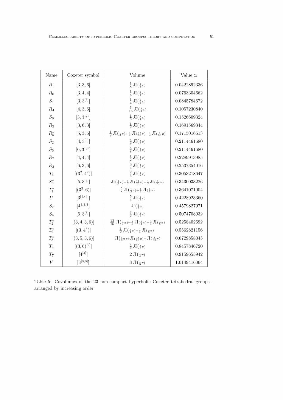
Commensurability of hyperbolic Coxeter groups: theory and computation 51
Name Coxeter symbol Volume Value '
R1 [3, 3, 6] 18 L( 1
3π) 0.0422892336
R6 [3, 4, 4] 16 L( 1
4π) 0.0763304662
S1 [3, 3[3]] 14 L( 1
3π) 0.0845784672
R4 [4, 3, 6] 516 L( 1
3π) 0.1057230840
S6 [3, 41,1] 13 L( 1
4π) 0.1526609324
R2 [3, 6, 3] 12 L( 1
3π) 0.1691569344
R∗5 [5, 3, 6] 12 L( 1
3π)+ 14 L( 11
30π)− 14 L( 1
30π) 0.1715016613
S2 [4, 3[3]] 58 L( 1
3π) 0.2114461680
S5 [6, 31,1] 58 L( 1
3π) 0.2114461680
R7 [4, 4, 4] 12 L( 1
4π) 0.2289913985
R3 [6, 3, 6] 34 L( 1
3π) 0.2537354016
T5 [(32, 42)] 23 L( 1
4π) 0.3053218647
S∗3 [5, 3[3]] L( 13π)+ 1
2 L( 1130π)− 1
2 L( 130π) 0.3430033226
T ∗1 [(33, 6)] 58 L( 1
3π)+ 13 L( 1
4π) 0.3641071004
U [3[ ]×[ ]] 54 L( 1
3π) 0.4228923360
S7 [41,1,1] L( 14π) 0.4579827971
S4 [6, 3[3]] 32 L( 1
3π) 0.5074708032
T ∗2 [(3, 4, 3, 6)] 1316 L( 1
3π)− 16 L( 1
4π)+ 23 L( 1
8π) 0.5258402692
T ∗6 [(3, 43)] 12 L( 1
4π)+ 23 L( 1
8π) 0.5562821156
T ∗3 [(3, 5, 3, 6)] L( 13π)+L( 11
60π)−L( 160π) 0.6729858045
T4 [(3, 6)[2]] 52 L( 1
3π) 0.8457846720
T7 [4[4]] 2L( 14π) 0.9159655942
V [3[3,3]] 3L( 13π) 1.0149416064
Table 5: Covolumes of the 23 non-compact hyperbolic Coxeter tetrahedral groups –
arranged by increasing order
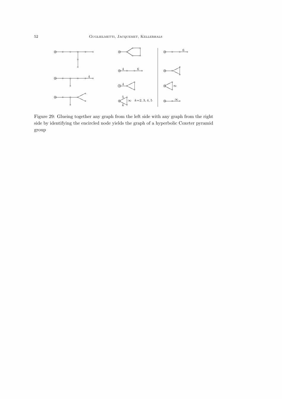
52 Guglielmetti, Jacquemet, Kellerhals
da a a aa aaHH
da a aa a a a4
da a a aaaa a da a aa aa
da a a a4 6
ea a aaHH
4
da aaHH5
k
k=2, 3, 4, 5∞
da a a a6
da a aaHH
da aaHH
∞
da a a∞
Figure 29: Glueing together any graph from the left side with any graph from the right
side by identifying the encircled node yields the graph of a hyperbolic Coxeter pyramid
group
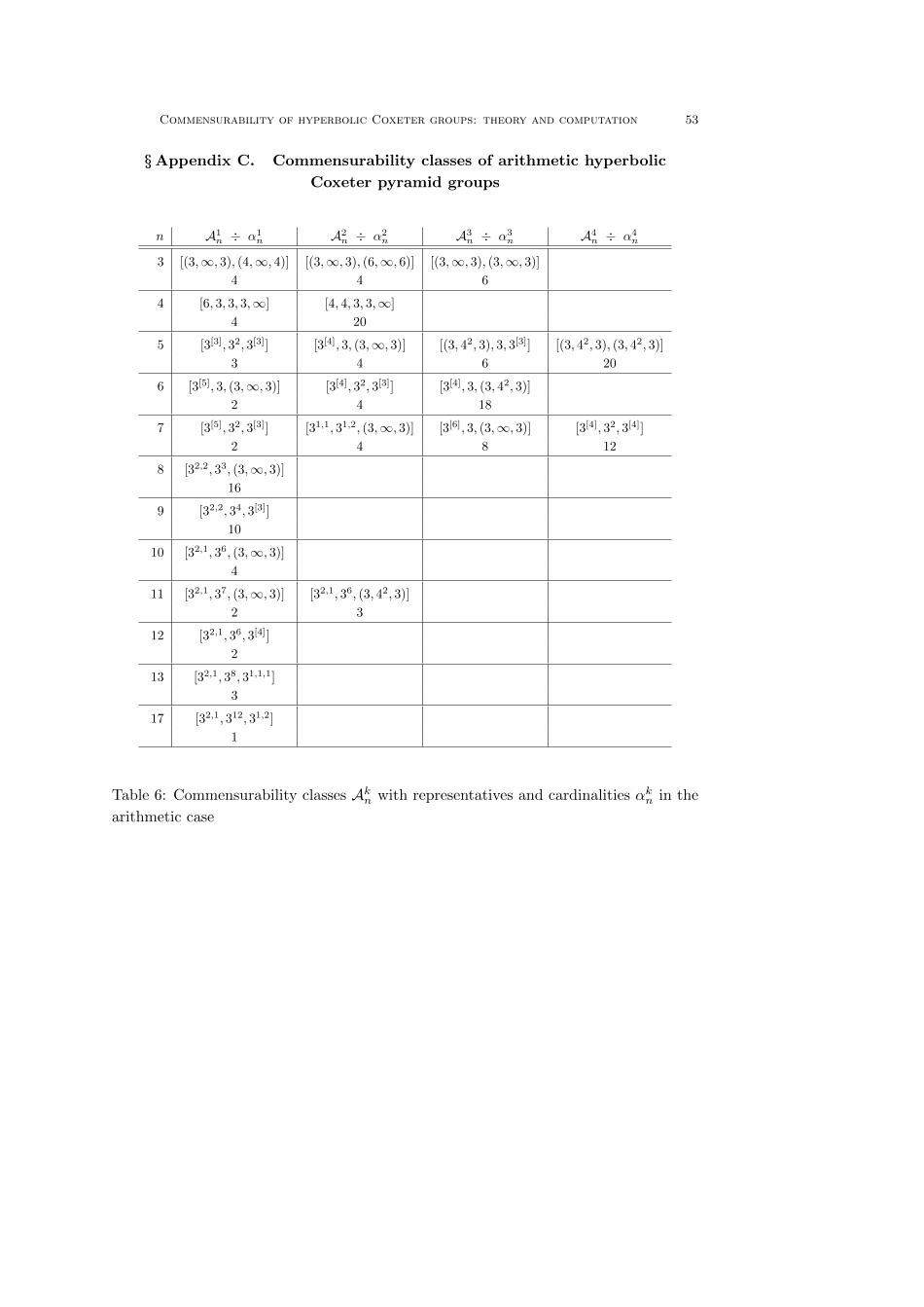
Commensurability of hyperbolic Coxeter groups: theory and computation 53
§Appendix C. Commensurability classes of arithmetic hyperbolic
Coxeter pyramid groups
n A1n ÷ α1
n A2n ÷ α2
n A3n ÷ α3
n A4n ÷ α4
n
3 [(3,∞, 3), (4,∞, 4)] [(3,∞, 3), (6,∞, 6)] [(3,∞, 3), (3,∞, 3)]
4 4 6
4 [6, 3, 3, 3,∞] [4, 4, 3, 3,∞]
4 20
5 [3[3], 32, 3[3]] [3[4], 3, (3,∞, 3)] [(3, 42, 3), 3, 3[3]] [(3, 42, 3), (3, 42, 3)]
3 4 6 20
6 [3[5], 3, (3,∞, 3)] [3[4], 32, 3[3]] [3[4], 3, (3, 42, 3)]
2 4 18
7 [3[5], 32, 3[3]] [31,1, 31,2, (3,∞, 3)] [3[6], 3, (3,∞, 3)] [3[4], 32, 3[4]]
2 4 8 12
8 [32,2, 33, (3,∞, 3)]
16
9 [32,2, 34, 3[3]]
10
10 [32,1, 36, (3,∞, 3)]
4
11 [32,1, 37, (3,∞, 3)] [32,1, 36, (3, 42, 3)]
2 3
12 [32,1, 36, 3[4]]
2
13 [32,1, 38, 31,1,1]
3
17 [32,1, 312, 31,2]
1
Table 6: Commensurability classes Akn with representatives and cardinalities αkn in the
arithmetic case
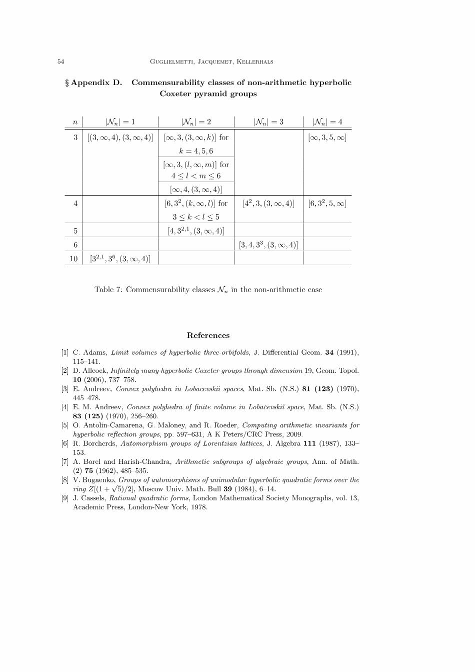
54 Guglielmetti, Jacquemet, Kellerhals
§Appendix D. Commensurability classes of non-arithmetic hyperbolic
Coxeter pyramid groups
n |Nn| = 1 |Nn| = 2 |Nn| = 3 |Nn| = 4
3 [(3,∞, 4), (3,∞, 4)] [∞, 3, (3,∞, k)] for [∞, 3, 5,∞]
k = 4, 5, 6
[∞, 3, (l,∞,m)] for
4 ≤ l < m ≤ 6
[∞, 4, (3,∞, 4)]
4 [6, 32, (k,∞, l)] for [42, 3, (3,∞, 4)] [6, 32, 5,∞]
3 ≤ k < l ≤ 5
5 [4, 32,1, (3,∞, 4)]
6 [3, 4, 33, (3,∞, 4)]
10 [32,1, 36, (3,∞, 4)]
Table 7: Commensurability classes Nn in the non-arithmetic case
References
[1] C. Adams, Limit volumes of hyperbolic three-orbifolds, J. Differential Geom. 34 (1991),
115–141.
[2] D. Allcock, Infinitely many hyperbolic Coxeter groups through dimension 19, Geom. Topol.
10 (2006), 737–758.
[3] E. Andreev, Convex polyhedra in Lobacevskii spaces, Mat. Sb. (N.S.) 81 (123) (1970),
445–478.
[4] E. M. Andreev, Convex polyhedra of finite volume in Lobacevskiı space, Mat. Sb. (N.S.)
83 (125) (1970), 256–260.
[5] O. Antolin-Camarena, G. Maloney, and R. Roeder, Computing arithmetic invariants for
hyperbolic reflection groups, pp. 597–631, A K Peters/CRC Press, 2009.
[6] R. Borcherds, Automorphism groups of Lorentzian lattices, J. Algebra 111 (1987), 133–
153.
[7] A. Borel and Harish-Chandra, Arithmetic subgroups of algebraic groups, Ann. of Math.
(2) 75 (1962), 485–535.
[8] V. Bugaenko, Groups of automorphisms of unimodular hyperbolic quadratic forms over the
ring Z[(1 +√
5)/2], Moscow Univ. Math. Bull 39 (1984), 6–14.
[9] J. Cassels, Rational quadratic forms, London Mathematical Society Monographs, vol. 13,
Academic Press, London-New York, 1978.
Commensurability of hyperbolic Coxeter groups: theory and computation 55
[10] H. S. M. Coxeter, Discrete groups generated by reflections, Ann. of Math. (2) 35 (1934),
588–621.
[11] M. Elia, C. Interlando, and R. Rosenbaum, On the Structure of Residue Rings of Prime
Ideals in Algebraic Number Fields–Part II: Ramified Primes, vol. 6, 2011, pp. 565–589.
[12] V. Emery, Even unimodular Lorentzian lattices and hyperbolic volume, J. Reine Angew.
Math. 690 (2014), 173–177.
[13] F. Esselmann, Uber kompakte hyperbolische Coxeter-Polytope mit wenigen Facetten, Ph.D.
thesis, 1994, Preprint / Universitat Bielefeld, Sonderforschungsbereich 343, Diskrete
Strukturen in der Mathematik ; 94-087, 68 pages.
[14] , The classification of compact hyperbolic Coxeter d-polytopes with d + 2 facets,
Comment. Math. Helv. 71 (1996), 229–242.
[15] A. Felikson and P. Tumarkin, On bounded hyperbolic d-dimensional Coxeter polytopes with
d+ 4 hyperfaces, Tr. Mosk. Mat. Obs. 69 (2008), 126–181.
[16] , On hyperbolic Coxeter polytopes with mutually intersecting facets, J. Combin.
Theory Ser. A 115 (2008), 121–146.
[17] , On simple ideal hyperbolic Coxeter polytopes, Izv. Ross. Akad. Nauk Ser. Mat. 72
(2008), 123–136.
[18] , Essential hyperbolic Coxeter polytopes, Israel J. Math. 199 (2014), 113–161.
[19] O. Goodman, D. Heard, and C. Hodgson, Commensurators of cusped hyperbolic manifolds,
Experiment. Math. 17 (2008), 283–306.
[20] M. Gromov and I. Piatetski-Shapiro, Nonarithmetic groups in Lobachevsky spaces, IHES
Publ. Math. (1988), no. 66, 93–103.
[21] F. Gueritaud, On an elementary proof of Rivin’s characterization of convex ideal hyperbolic
polyhedra by their dihedral angles, 108 (2004), 111–124.
[22] R. Guglielmetti, CoxIter - Computing invariants of hyperbolic Coxeter groups, LMS J.
Comput. Math. 18 (2015), 754–773.
[23] , Hyperbolic isometries in (in-)finite dimensions and discrete reflection groups:
theory and computations, Ph.D. thesis, University of Fribourg, 2017.
[24] R. Guglielmetti, M. Jacquemet, and R. Kellerhals, On commensurable hyperbolic Coxeter
groups, Geom. Dedicata 183 (2016), 143–167.
[25] H.-C. Im Hof, Napier cycles and hyperbolic Coxeter groups, Bull. Soc. Math. Belg. Ser. A
42 (1990), 523–545.
[26] M. Jacquemet, The inradius of a hyperbolic truncated n-simplex, Discrete Comput. Geom.
51 (2014), 997–1016.
[27] , New contributions to hyperbolic polyhedra, reflection groups, and their com-
mensurability, Ph.D. thesis, PhD Thesis No 1929, Universite de Fribourg, 2015,
https://doc.rero.ch/record/257511.
[28] , On hyperbolic Coxeter n-cubes, European J. Combin. 59 (2017), 192–203.
[29] N. Johnson, R. Kellerhals, J. Ratcliffe, and S. Tschantz, The size of a hyperbolic Coxeter
simplex, Transform. Groups 4 (1999), 329–353.
[30] , Commensurability classes of hyperbolic Coxeter groups, Linear Algebra Appl. 345
(2002), 119–147.
[31] N. Johnson and A. Weiss, Quaternionic modular groups, Linear Algebra Appl. 295 (1999),
159–189.
[32] I. Kaplinskaja, The discrete groups that are generated by reflections in the faces of simpli-
cial prisms in Lobacevskiı spaces, Mat. Zametki 15 (1974), 159–164.
[33] A. Karrass and D. Solitar, The subgroups of a free product of two groups with an amalga-
56 Guglielmetti, Jacquemet, Kellerhals
mated subgroup, Trans. Amer. Math. Soc. 150 (1970), 227–255.
[34] R. Kellerhals, On the volume of hyperbolic polyhedra, Math. Ann. 285 (1989), 541–569.
[35] T.-Y. Lam, Introduction to quadratic forms over fields, Graduate Studies in Mathematics
ed., vol. 67, American Mathematical Soc., 2005.
[36] C. Maclachlan, Commensurability classes of discrete arithmetic hyperbolic groups, Groups
Geom. Dyn. 5 (2011), 767–785.
[37] C. Maclachlan and A. Reid, Invariant trace-fields and quaternion algebras of polyhedral
groups, J. London Math. Soc. (2) 58 (1998), 709–722.
[38] , The arithmetic of hyperbolic 3-manifolds, Graduate Texts in Mathematics, vol.
219, Springer-Verlag, New York, 2003.
[39] G. Maxwell, Euler characteristics and imbeddings of hyperbolic Coxeter groups, J. Austral.
Math. Soc. Ser. A 64 (1998), 149–161.
[40] J. Mcleod, Hyperbolic Coxeter pyramids, Advances in Pure Mathematics 3 (2013), 78–82.
[41] A. Merkurjev, On the norm residue symbol of degree 2, Soviet Math. Dokl. 24 (1982),
1546–1551.
[42] R. Meyerhoff, The cusped hyperbolic 3-orbifold of minimum volume, Bull. Amer. Math.
Soc. (N.S.) 13 (1985), 154–156.
[43] J. Milnor, On polylogarithms, Hurwitz zeta functions, and the Kubert identities, Enseign.
Math. (2) 29 (1983), 281–322.
[44] W. Neumann and A. Reid, Arithmetic of hyperbolic manifolds, Topology ’90 (Columbus,
OH, 1990), Ohio State Univ. Math. Res. Inst. Publ., vol. 1, de Gruyter, Berlin, 1992,
pp. 273–310.
[45] M. Prokhorov, Absence of discrete reflection groups with non-compact fundamental poly-
hedron of finite volume in Lobachevskij spaces of large dimension, Mathematics of the
USSR-Izvestiya 28 (1987), 401–411.
[46] I. Rivin, A characterization of ideal polyhedra in hyperbolic 3-space, Ann. of Math. (2)
143 (1996), 51–70.
[47] R. Roeder, Andreev’s classification of hyperbolic polyhedra, PhD Thesis, Universite de
Provence, Marseille, 2004.
[48] R. Roeder, J. Hubbard, and W. Dunbar, Andreev’s theorem on hyperbolic polyhedra, 57
(2007), no. 3, 825–882.
[49] L. Schlettwein, Hyperbolische Simplexe, Diploma Thesis, University of Basel, 1995.
[50] J.-P. Serre, A course in arithmetic, vol. 7, Springer-Verlag, New York, 1996.
[51] W. Thurston, The geometry and topology of three-manifolds, url-
http://library.msri.org/books/gt3m/PDF/7.pdf, 1980.
[52] P. Tumarkin, Hyperbolic Coxeter n-polytopes with n+2 facets, arXiv:math/0301133 (2003),
14 pp.
[53] , Non-compact hyperbolic Coxeter n-polytopes with n + 3 facets, Russian Math.
Surveys 58 (2003), 805–806.
[54] , Hyperbolic Coxeter polytopes in Hm with n + 2 hyperfacets, Mat. Zametki 75
(2004), 909–916.
[55] , Compact hyperbolic Coxeter n-polytopes with n + 3 facets, Electron. J. Combin.
14 (2007), no. 1, Research Paper 69, 36 pp. (electronic).
[56] M.-F. Vigneras, Arithmetique des algebres de quaternions, vol. 800, Springer-Verlag, 1980.
[57] E. Vinberg, Discrete groups generated by reflections in Lobacevskii spaces, Sbornik 1
(1967), 429–444.
[58] , On groups of unit elements of certain quadratic forms, Sbornik 16 (1972), 17–35.
Commensurability of hyperbolic Coxeter groups: theory and computation 57
[59] , Hyperbolic reflection groups, Russian Mathematical Surveys 40 (1985), 31–75.
[60] , Non-arithmetic hyperbolic reflection groups in higher dimensions, Univ. Bielefeld
Preprint 14047 (2014), 10 pp.
[61] E. Vinberg and O. Shvartsman, Discrete groups of motions of spaces of constant curvature,
Geometry, II, Encyclopaedia Math. Sci., vol. 29, Springer, Berlin, 1993, pp. 139–248.


