DI
SC
US
SI
ON
P
AP
ER
S
ER
IE
S
Forschungsinstitut zur Zukunft der ArbeitInstitute for the Study of Labor
Child Labor and Trade Liberalization in Indonesia
IZA DP No. 4376
August 2009
Krisztina Kis-KatosRobert Sparrow
Child Labor and Trade Liberalization
in Indonesia
Krisztina Kis-Katos University of Freiburg
Robert Sparrow
Erasmus University Rotterdam and IZA
Discussion Paper No. 4376 August 2009
IZA
P.O. Box 7240 53072 Bonn
Germany
Phone: +49-228-3894-0 Fax: +49-228-3894-180
E-mail: [email protected]
Any opinions expressed here are those of the author(s) and not those of IZA. Research published in this series may include views on policy, but the institute itself takes no institutional policy positions. The Institute for the Study of Labor (IZA) in Bonn is a local and virtual international research center and a place of communication between science, politics and business. IZA is an independent nonprofit organization supported by Deutsche Post Foundation. The center is associated with the University of Bonn and offers a stimulating research environment through its international network, workshops and conferences, data service, project support, research visits and doctoral program. IZA engages in (i) original and internationally competitive research in all fields of labor economics, (ii) development of policy concepts, and (iii) dissemination of research results and concepts to the interested public. IZA Discussion Papers often represent preliminary work and are circulated to encourage discussion. Citation of such a paper should account for its provisional character. A revised version may be available directly from the author.
IZA Discussion Paper No. 4376 August 2009
ABSTRACT
Child Labor and Trade Liberalization in Indonesia* We examine the effects of trade liberalization on child work in Indonesia. Our estimation strategy identifies geographical differences in the effects of trade policy through district level exposure to reduction in import tariff barriers. We use a balanced panel of 261 districts, based on four rounds (1993 to 2002) of the Indonesian annual national household survey (Susenas), and relate workforce participation of children aged 10-15 to geographic variation in relative tariff exposure. Our main findings show that increased exposure to trade liberalization is associated with a decrease in child work among the 10 to 15 year olds. The effects of tariff reductions are strongest for children from low skill backgrounds and in rural areas. Favorable income effects for the poor, induced by trade liberalization, are likely to be the dominating effects underlying these results. JEL Classification: J13, O24, O15 Keywords: child labor, trade liberalization, poverty, Indonesia Corresponding author: Robert Sparrow Institute of Social Studies Erasmus University Rotterdam P.O. Box 29776 2502 LT The Hague The Netherlands E-mail: [email protected]
* We thank Arjun Bedi, Sebi Buhai, Eric Edmonds, Pedro Goulart, Michael Grimm, Umbu Reku Raya, Günther Schulze and Bambang Sjahrir Putra for useful comments and discussions, as well as seminar and conference participants at Aarhus School of Business, Freiburg University, Institute of Social Studies, the Second IZA Workshop on Child Labor in Developing Countries, and the Fourth Annual Conference of the German Research Committee on Development Economics. All errors are our own.
1 Introduction
The effects of trade liberalization on child labor are widely debated and public and
political interest in the issue is high. From a theoretical perspective these effects
are a priori unclear (e.g., Ranjan 2001, Jafarey and Lahiri 2002) as trade liber-
alization acts potentially through several channels, changing relative prices, real
income distribution, wages and net returns to education. The arising income and
substitution effects can both raise and reduce workforce participation of children.
Empirical evidence on the issue is scarce. Cross-country studies generally find
trade liberalization to be associated with lower incidence of child labor on average
(Cigno, Rosati and Guarcello 2002), a relationship that seems most likely to be
driven by the effect of trade on income, as more open economies have less child la-
bor because they are richer (Edmonds and Pavcnik 2006). Kis-Katos (2007) finds
differential effects of trade openness, with smaller reductions in child labor for the
poorest food exporting countries. However, empirical studies based on micro data
and direct evidence from trade reforms are required to understand the heteroge-
nous effects from trade liberalization and identify the main channels at work. For
example, Edmonds and Pavcnik (2005b) find that rice price increases due to a
dismantling of export quotas in Vietnam led to an overall decrease in child labor
in the 1990s, especially due to the relatively evenly distributed favorable income
effects. In contrast, Edmonds, Pavcnik and Topalova (2007) find that in rural
India, districts that have been more strongly exposed to trade liberalization have
experienced smaller increases in school enrollment on average, which they argue
is primarily due to the unfavorable income effects to the poor and the relatively
high costs of education in these districts.
This study contributes to the empirical micro literature by examining the trade
2
liberalization experience of Indonesia in the 1990s, which, given the vast geographic
heterogeneity of the archipelago, offers an interesting case study on the effects of
trade liberalization on child work. In preparation to and following its accession
to the WTO, Indonesia went through a major reduction in tariff barriers: average
import tariff lines decreased from around 19.4 percent in 1993 to 8.8 percent in
2002. During that same period the workforce participation of children aged 10
to 15 years more than halved. Due to Indonesia’s size and geographic variation
in economic structure, the various districts have been very differently affected by
trade liberalization, which offers us a valuable identification strategy.
Our identification strategy follows that of Topalova (2005) and Edmonds et al.
(2007), as we combine geographic variation in sector composition of the economy
and temporal variation in tariff lines by product category, yielding geographic vari-
ation in (changes in) average exposure to trade liberalization over time. We extend
this approach in several ways. First, we define two alternative measures of geo-
graphic exposure to trade liberalization, by weighting tariffs on different products
by the shares these sectors take in (i) regional GDP, and (ii) the regional struc-
ture of employment. These measures reflect different dimensions of households’
exposure to trade liberalization: the former through the distributional effects of
local economic growth, the latter through labor market dynamics. In addition to
this, the data allows us to go beyond the fixed effects approach employed in earlier
studies and investigate the dynamic effects of trade liberalization.
The analysis draws on a variety of data sources. Indonesia’s annual national
household survey (Susenas) provides information on the main activities of chil-
dren and their basic socio-economic characteristics. We use four rounds of this
repeated cross section data, spaced at 3–year intervals between 1993 and 2002.
As the Susenas is representative at the district level, we apply our analysis both
3

at the individual level using pooled repeated cross section data with district fixed
effects, and at the district level with pseudo panel data for 261 districts. The data
on economic structure of the districts comes from information on regional GDP
(GRDP) of the Central Bureau of Statistics in Indonesia (BPS), while district-
level employment shares and further controls are based on Susenas. Additional
district–level information is derived from PODES, the Village Potential Census.
Finally, information on tariff lines comes from the UNCTAD–TRAINS database.
We find that stronger exposure to trade liberalization has lead to a decrease
in child labor among the 10 to 15 year olds. The effects are strongest for children
from low skill backgrounds and in rural areas. Favorable income effects for the poor
induced by trade liberalization are likely to be the dominating effects underlying
these results.
The next section of the paper provides a theoretical framework for our analysis.
The third section elaborates on the context of the tariff reductions in Indonesia,
and the developments in child labor for our study period. Section 4 presents the
data and sets out the identification strategy. The results are then discussed in
section 5 while section 6 concludes.
2 Theoretical background
Although child labor is determined by an interaction between the necessity and
the opportunities to work, credit constraints, returns to school, as well as parental
preferences, its close link to poverty is undisputed (Edmonds and Pavcnik 2005a).
Hence, reductions in trade barriers are more likely to lead to reductions in child
labor if they are going to benefit the poor in the economy. Based on standard
Stolper–Samuelson reasoning, trade liberalization has been commonly expected
4

to alleviate poverty in developing countries (e.g., Bhagwati and Srinivasan 2002).
However, if specialization in production also increases the demand for unskilled
labor, the overall effects on child labor are a priori not clear.
Even in its simplest version, the Stolper–Samuelson reasoning does not neces-
sarily imply a reduction in child labor due to trade liberalization, as the resulting
income and substitution effects point into different directions. In a Heckscher–
Ohlin economy with two mobile factors, low and high skilled labor, and two in-
dustries producing one export and one import-competing good, reducing import
tariffs leads to a decrease in the relative price of the imported good with respect to
the numeraire (export good). On the production side, there will be a shift towards
the production of exportables with low skill intensity, which in turn raises the
demand for unskilled labor and reduces the skill premium in the economy.1 The
price changes will also lead to consumption shifts, and the overall effects of trade
liberalization are expected to be positive (gains from trade). Households will be
affected by changing goods and factor prices through two main channels. First,
changes in wages and goods prices alter the real income of the households. Second,
shifts in the relative prices of goods and opportunity costs of not working result
in substitution effects which lead to a further reallocation of consumption and la-
bor supply. While real incomes of the poor low–skilled households should increase
after trade liberalization, the overall reaction of child labor is not clear–cut, since
rising real wages of the unskilled increase the incentives to work.
More formally, consider a household consisting of one child and one adult where
the adult chooses consumption of two goods (𝑐1, 𝑐2), and allocates the child’s time
1 These price effects might be both mitigated and enhanced in the presence of non–tradablegoods: If the import-competing sector is more capital intensive than both the exporting andthe non-traded sectors (as it might be expected in a developing economy), the relative price ofthe non–traded good with respect to the numeraire (exportable) will rise. Overall demand andproduction shifts will in this case depend on the relative factor intensities of each industry andthe gross substitutability of all goods in consumption (Komiya 1967).
5
between work (𝑙), and schooling (1 − 𝑙) in order to maximize household utility.
The utility of schooling (𝜈(1 − 𝑙)) reflects both disutility of child labor and the
discounted present value of the returns to school. The decision is made subject to
the household’s budget constraint and the time constraints for the child, assum-
ing that financial markets are typically imperfect such that the household cannot
borrow against the child’s future income in order to invest into education, even if
the discounted net returns to education would be positive.2 The budget constraint
states that the expenditures on consumption goods and schooling (𝜎(1−𝑙))3 cannotbe higher than the adult’s income (𝑦) plus the income from child labor (𝛾𝑤𝑙).4
max𝑐1,𝑐2,𝑙
𝑢(𝑐1, 𝑐2) + 𝜈(1− 𝑙) s.t. 𝑦 + 𝛾𝑤𝑙 = 𝑝𝑐1 + 𝑐2 + 𝜎(1− 𝑙), 0 ≤ 𝑙 ≤ 1
The relative price of the importables (𝑐1) is denoted by 𝑝, unskilled wages by 𝑤.
The child is assumed to be a perfect although less productive (𝛾 < 1) substitute
for unskilled adult labor (substitution axiom by Basu and Van 1998). Given the
optimal allocation of income over the two consumption goods, optimal (uncom-
pensated) child labor supply (𝑙∗) is determined by relative goods and factor prices,
school costs and adult income:
𝑙∗ = 𝑙(𝑝, 𝑤𝛾, 𝜎, 𝑦) (1)
For an interior solution (where the child combines work and schooling), the opti-
2 Credit constraints and imperfect smoothing seem a reasonable assumption for most develop-ing countries, at least for those households that send their children to work, as credit constraintsare among the main causes for child labor (e.g., Beegle, Dehejia and Gatti 2006). For IndonesiaKis-Katos and Schulze (2009) show that credit availability is closely related to the incidence ofchild labor in small businesses.
3The direct costs of schooling (excluding opportunity costs) are denoted by 𝜎, and for sim-plicity, are assumed to be linear in school time.
4 If the adult is unskilled, adult income equals the unskilled wage 𝑦 = 𝑤, if the adult is skilled,adult income equals the skilled wage. In both cases adult labor is assumed to be inelastic insupply.
6

mality condition is given by:
𝑤𝛾 𝑣𝑦(𝑝, 𝑤𝛾, 𝜎, 𝑦) = 𝜈′(1− 𝑙)− 𝜎 𝑣𝑦(𝑝, 𝑤𝛾, 𝜎, 𝑦) (2)
which is expressed in terms of an indirect utility function (𝑣(𝑝, 𝑤𝛾, 𝜎, 𝑦)). The
work–school trade–off depends thus on the relative magnitudes of the real value
of the marginal product of child labor (left hand side of equation (2)) and the net
real marginal returns to education (right hand side of equation (2)), with marginal
utility of income (𝑣𝑦) denoting the inverse of the price deflator. A child will be
doing at least some work, if real child wages are greater than the marginal real net
return to education if the child spends all its available time on learning (𝑙 = 0).5
After reducing import tariffs, imported and import competing products become
relatively less expensive (𝑑𝑝 < 0), the overall effect of which can be seen by totally
differentiating the uncompensated child labor supply equation (1):
𝑑𝑙∗ =( ∂𝑙
∂𝑝︸︷︷︸−?
+𝛾∂𝑙
∂𝑤︸︷︷︸+?
∂𝑤
∂𝑝︸︷︷︸−
+∂𝑙
∂𝑦︸︷︷︸−
∂𝑦
∂𝑝︸︷︷︸−?
)𝑑𝑝 (3)
The first term within the parentheses captures the direct effects of a price
increase and is negative if schooling and the import competing good are gross sub-
stitutes: As schooling becomes relatively less expensive, child labor will decrease
but the substitution effect is (partly) counteracted by a decrease in real income
due to the price increase. The first part of the second term captures both the
income and substitution effects from an increase in child wages: if the substitution
effect dominates, rising wages increase child labor supply.6 The second part of
5 Conversely, a child will be spending at least some time going to school if real child wagesare smaller than the marginal net returns to education at no schooling (𝑙 = 1). For expositionalease we abstract from the possibility that a child stays idle, which will be most likely if both realnet returns to education and value of marginal product of child work are low.
6 Additionally, there might be dynamic effects of falling skill premia, which make investmentinto education less profitable, reduce 𝜈′(1− 𝑙) and thus raise ∂𝑙/∂𝑤 further. But as technological
7

the term captures the change in unskilled wages with an increase in import prices
and is negative by a Stolper–Samuelson argument. The third term captures the
effect through adult income: if the adult has unskilled labor, an increase in the
import price should decrease adult income, and hence increase child labor. The
overall sign of these effects depends on whether the favorable income effects or
the substitution effects are dominating.7 Departures from the Stolper–Samuelson
reasoning that result additionally in negative income effects for the poor make an
increase in child labor more likely.
The expected favorable effects of trade liberalization on child labor depend
strongly on the presence of Stolper–Samuelson linkages which has been widely
questioned over the last decades, both on theoretical and empirical grounds. The-
oretically, the Stolper–Samuelson conclusions fail to hold for many real–world rele-
vant departures from the simplest framework (e.g., Davis and Mishra 2007). Split-
ting “the rest of the world” into multiple trading partners reveals that a developing
country might trade both with more and less skill–abundant countries than itself,
in which case reductions in tariffs on goods with low–skill intensity might also
hurt the poor. The poor will suffer also if the effects of trade liberalization are ac-
companied and even dominated by skill biased technological change. In contrast,
reductions in tariffs on goods that are not produced within a country will have no
effects on protection and will only benefit consumers of those goods.
Favorable income effects are more likely to occur if intersectoral worker mo-
bility is high and markets are competitive, which corresponds to a longer run
upgrading is certainly an issue in the long run, this gives an additional motive for human capitalaccumulation and makes the longer term relevance of short term falls in skill premia questionable.
7 Although the above arguments have been presented on the intensive margin (with bothwork and school being interior), the effects translate easily to the extensive margin as well: Theworkforce participation of a child is influenced through the same channels as presented above,and the share of children working and/or enrolled at school is influenced by changes in districtpoverty and wages/labor market conditions, and hence by the same income and substitutioneffects.
8

perspective. If workers’ skills are industry specific instead and hence the between
industry mobility is low, workers might be harmed in the short run by reductions
in protection. In a constrained economic environment, with imperfect smoothing,
such short term economic shocks can also have long term consequences for the
poor. For instance, decisions on withdrawing a child from school in face of a shock
are often irreversible and can have intergenerational effects.
Empirical evidence on the effects of globalization on poverty is also inconclu-
sive, since, contrary to the Stolper–Samuelson predictions, many empirical studies
do not observe reductions either in poverty or in wage inequality in developing
countries that reduced tariffs unilaterally (e.g., Harrison 2007).8 For Indonesia,
however, the pro–poor effects of trade liberalization are not unlikely: Suryahadi
(2001) documents rising unskilled wages over the period of trade liberalization
in the 1990s, while Sitalaksmi, Ismalina, Fitrady and Robertson (2007) find im-
provements in perceived working conditions. Indeed, our results seem to suggest
that tariff reductions have induced income effects and reduced poverty, eventually
leading to a reduction in rural child labor.
Our empirical analysis will focus on child labor and not on schooling, since
consistent data on school attendance is not available for the study period (see also
the data section). In addition, we will not consider the effects of trade liberaliza-
tion propagated through changes in consumption patterns, but only analyze the
channels associated with the composition of economic activity.9
8 Reductions in protection are more likely to benefit the poor if labor mobility between indus-tries is high and labor market policies are flexible, and if social safety nets are well–functioning(Harrison 2007).
9 For our empirical strategy this implicitly implies that differences in district–level trends inthe composition of consumption are assumed to be unrelated to the districts’ economic productionstructure; in which case not controlling for the consumption channel will not confound ourestimates.
9
3 Trade liberalization and children in Indonesia
3.1 Trade liberalization in the 1990s
Trade liberalization in Indonesia took place over more than fifteen years. From the
mid-1980s the former import substitution policy has been gradually replaced by a
less restrictive trade regime, tariff lines have been reduced while at the same time
a slow tarification of non–tariff barriers took place (Basri and Hill 2004). This
laid the ground to the next wave of trade liberalization in the mid–1990s, with ris-
ing foreign firm ownership and increasing export and import penetration.10 Tariff
reductions were particularly strong in the 1990s, with Indonesian trade liberaliza-
tion policy in that decade being defined by two major events: the conclusion of the
Uruguay round in 1994 and Indonesia’s commitment to multilateral agreements
on tariff reductions, and the Asian economic crisis in 1997 and the post-crisis re-
covery process. After the Uruguay round Indonesia committed itself to reduce all
of its bound tariffs to less than 40% within ten years. In May 1995 a large package
of tariff reductions was announced which laid down the schedule of major tariff
reductions until 2003, and implemented further commitments of Indonesia to the
Asia Pacific Economic Cooperation (Fane 1999). While the removal of specific
non–tariff barriers was accompanied by a temporary rise in tariffs (especially in
the food manufacturing sector), this did not affect the overall declining trend in
any major way.
Figure 1 shows the reduction in tariff lines over time and the variation between
industries. On average, nominal tariffs reduced from 17.2 percent in 1993 to 6.6
percent in 2002. In this period the strongest reductions occurred from 1993 to
10 Arguably, cronyism and specific protection of a few industries with ties to the Soeharto–family—especially chemicals, motor vehicles and steel—reduced the effect of overall liberalization.However, the largest part of the cronyism occurred in nontraded sectors and did not further affectprotection of the traded sectors (Basri and Hill 2004, p.637).
10
1995 and during the post crisis period after 1999. Tariff dispersion decreased
especially in the post–crisis period when reductions were more universal. While
tariffs decreased across the board, there were marked differences in initial levels and
in the extent of the decrease (see Figure 2). Manufacturing started with relatively
high tariff barriers but also showed the strongest reductions. For example, wood
and furniture saw tariffs decline from 27.2 to 7.9 percent, textiles form 24.9 to 8.1
percent and other manufacturing from 18.9 to 6.4 percent. The average tariffs for
agriculture were already much lower in 1993, at 11.5, and which reduced to 3.0
percent.11
Existing studies on the effects of Indonesian trade liberalization document both
increased firm productivity and improvements of working conditions in manufac-
turing. At the plant–level, Amiti and Konings (2007) find that trade liberalization
affected firms’ productivity through two main channels: falling tariffs on imported
inputs fostered learning and raised both product quality and variety, while falling
output protection increased the competitive pressures. Comparing the two effects
they argue that gains from falling input tariffs were considerably higher. Firm
productivity has also been strongly affected by FDI flows, as firms with increas-
ing foreign ownership experienced restructuring, employment and wage growth,
as well as stronger linkages to export and import markets (Arnold and Smarzyn-
ska Javorcik 2005). At the same time, working conditions seem to have improved,
especially in manufacturing. Using individual employment data, Sitalaksmi et al.
(2007) argue that the increase in export–oriented foreign direct investment went
along with rising relative wages in the textile and apparel sector. Additionally,
working conditions, proxied by workers’ own assessment of their income, work-
ing facilities, medical benefits, safety considerations and transport opportunities,
11 Figure 3 shows that tariff reductions and tariff levels are reasonably positively related; alloutliers showing significant increases in tariffs are related to alcoholic beverages and soft drinksthat were subject to a major retarification of non-tariff barriers.
11
improved over time in the expanding manufacturing industries as compared to
agriculture.
Based on a microsimulation exercise Hertel, Ivanic, Preckel and Cranfield
(2004) argue that full multilateral trade liberalization is expected to decrease
household poverty in Indonesia, although self-employed agricultural households
would be the most likely losers of trade liberalization in the short–run, which is
mainly due to the assumption that self-employed labor is immobile in the short–
run. In the longer run some former agricultural workers will be moving into the
formal wage labor market and the poverty headcount could be expected to fall for
all sectors. However, the mobility of low skill labor, and hence the speed and abil-
ity to exploit the opportunities from trade liberalization, may be underestimated
by Hertel et al. (2004). For example, Suryahadi, Suryadarma and Sumarto (2009)
show that during the 1990s the agriculture employment share dropped from 50 to
40 percent, while the services share increased from 33 to 42 percent. In addition,
they attribute most of the poverty reductions in that decade to growth in urban
services. This is further supported by Suryahadi (2001), who documents a fast
increase in the employment of skilled labor force as well as a decline in wage in-
equality (i.e. faster wage growth for the unskilled) during trade liberalization in
Indonesia, although he does not establish causality.
3.2 Child work
Indonesia experienced a steady decline in child work in the thirty years before the
Indonesian economic crisis, but this decline halted with the onset of the crisis (e.g.,
Suryahadi, Priyambada and Sumarto 2005). Nevertheless, market work among
children aged 10 to 15 increased only slightly in response to the economic crisis
12
(e.g., Cameron 2001).12 During the crisis children have been moving out of the
formal wage employment sector into other small-scaled activities (Manning 2000),
but the labor supply response seems to be concentrated with older cohorts.
The overall decline in child work over the study period is portrayed in Figure
4, for boys and girls, and by different age groups. Child work is here defined as
any work activity that contributes to household income. From 1993 to 2002, the
incidence of child work halves for children of junior secondary school age (13 to
15 years old), and is cut by more than 70 percent for children age 10 to 12. This
decline is observed for both boys and girls, although boys engage in market work
more than girls. In 2002 market work incidence for boys age 13 to 15 years is
14.8 percent, and 2.3 percent for boys at age 10 to 12. Among girls market work
incidence is 10.0 and 1.6 percent for the same age groups, respectively.
Agriculture is the main sector for child work, and developments in this sector
are driving the overall trends, as shown in Figure 5. In 1993 just over 75 percent
of child work in the age group 10 to 12 occurred in agriculture, while two in
three child workers aged 13 to 15 worked in agriculture. The dominance of the
agricultural sector in child work translates into a 79 and 69 percent share in the
overall reduction in child work for the two age groups, respectively. However, the
relative changes from 1993 to 2002 are remarkably constant across sectors.
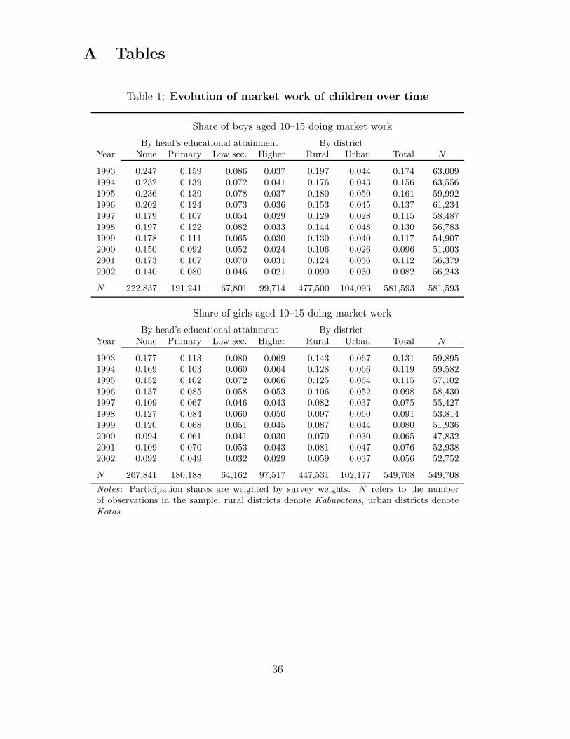
The trends in child work vary greatly by location and education attainment of
the head of household (Table 1). Child work incidence is much higher in rural dis-
tricts compared to municipalities, but rural areas experienced the largest decline,
both in absolute and relative terms. These patterns mirror the trend dominance of
the agricultural sector. Child work incidence decreases with the level of education
of the head of household. Boys living in households where the head of household
12 Information on working children below the age of 10 is not available at a systematic basis.
13

has not finished primary education, are almost 6 times more likely to work than
boys from households where the head of household holds a degree higher than ju-
nior secondary school; for girls this ratio is about 3. For all the levels of education
we see child work incidence decreasing.
In line with the trends in child labor, Indonesia has shown strong improve-
ments in education attainment over past decades, reaching almost universal pri-
mary school enrollment already in the mid 1980s (e.g., Jones and Hagul 2001, Lan-
jouw, Pradhan, Saadah, Sayed and Sparrow 2002). Indonesia’s current 9 year basic
education policy aims at achieving universal enrollment for children up to the age
of 15; that is, up to junior secondary school. But while junior secondary school
enrollment has certainly improved, the large drop out of around 30 percent in the
transition from primary to junior secondary (around 70 percent) remains a prob-
lem. In particular striking are the relatively low transition rates among the poor.
Among the poorest 20 percent of the population, almost half of the children that
finish primary school drop out at junior secondary level; this is in stark contrast to
the 12 percent drop out rate for the richest quintile (Paqueo and Sparrow 2006).
Other problems that are still cause for concern are delayed enrollment and rela-
tively high repetition rates, teacher quality and absenteeism, and lack of access to
secondary schools in remote and rural areas (World Bank 2006).
In the remainder of this analysis we focus on child work activities by primary
school age children close to the transition point, age 10 to 12, and junior secondary
school age children, age 13 to 15. For children younger than 10 information on
work is not available.
14

4 Data and empirical approach
4.1 Data
Indonesia’s national socio-economic household survey, Susenas, provides informa-
tion on the outcome variables and socio-economic characteristics for individuals
and households. The Susenas is conducted annually around January-February,
typically sampling approximately 200,000 households, and is representative at the
district level. The district will be our main unit of analysis, as districts take a key
role as the main administrative units in Indonesia, and the regional labor markets
are also best defined in district terms.
Districts are defined as municipalities (Kota) or predominantly rural areas
(Kabupaten). Each district (both the Kota and Kabupaten) can be further divided
into urban precincts (Kelurahan) and rural villages (Desa). It is important to
emphasize the difference between these two urban/rural indicators, since we will
use both variables in our analysis. A district classified as a rural Kabupaten mainly
consists of rural villages, but may also include small towns that are registered as
urban precincts in the data. In similar vein, districts classified as urban Kota
mainly contain urban precincts and neighborhoods, but may also cover some rural
areas at the fringes, which are then registered as villages. The exception are the
five districts comprising the capital Jakarta, which are defined completely as urban.
The Kota/Kabupaten classification will therefore appear as a fixed effect in our
analysis, but we will also investigate the differential effects of tariff reduction for
municipalities and rural districts. In addition, we will include the Desa/Kelurahan
division as time variant control variable within districts.
The outcome variables record whether a child has worked in the last week.
As mentioned earlier, market work is defined as activities that directly generate
15
household income, irrespectively of whether it was performed at the formal labor
market or within the family. We distinguish it from domestic work which consists
of household chores only. The Susenas also provides information on education at-
tainment of other household members, household composition, monthly household
expenditure and sector of employment.13
The sectoral share of GDP per district is derived from the Regional GDP
(GRDP) data of the Central Bureau of Statistics in Indonesia (BPS). The dis-
trict GRDP are available from 1993 onward, and breaks down district GDP by
1 digit sector, of which the tradable sectors are agriculture, manufacturing and
mining/quarrying. Information at lower level of aggregation is available (down to
3 digits), but the availability is not consistent over time.
Information on tariff lines comes from the UNCTAD–TRAINS database. These
reflect the simple average of all applied tariff rates, which tend to be substantially
lower than the bound tarrifs during the 1990s (WTO 1998, WTO 2003). As
data on tariff lines is not available for some years (1994, 1997, and 1998), we use
information from four three–year intervals (1993, 1996, 1999, and 2002) both in
the pooled cross section and in the district panel. We can consistently match the
relevant product categories to sectoral employment data derived from Susenas and
the GRDP sectors at the 1 digit level.
We cannot include every district in our sample: Districts in Aceh, Maluku and
Irian Jaya have not been included in the Susenas in some years due to violent
conflict situations at the time of the survey. In addition, the 13 districts in East
Timor were no longer covered by Susenas after the 1999 referendum on indepen-
dence. We therefore drop these regions from the analysis. Another problem is that
13 The Susenas also collects data on schooling. But, unfortunately, the data on school atten-dance (which refers to the same recall period as the questions on child work activities) can not beused for this study as it is not consistent over time due to changes in the questionnaire between1996 and 1999.
16
over the period 1993 to 2002 some districts have split up over time. To keep time
consistency in the district definitions, we redefine the districts to the 1993 parent
district definitions.
Since the Susenas rounds are representative for the district population in each
year, we construct a district panel by pooling the four annually repeated cross sec-
tions. This yields a balanced panel of 261 districts, which reduces to 244 districts
when we merge the GRDP data, as GRDP information is not available for all
districts. In addition to the pooled data, we also create a district pseudo-panel by
computing district–level means for each variable, weighted by survey weights. The
advantage of pooling the cross-section data is that we can work with individual
level data and can account for individual heterogeneity, both in terms of charac-
teristics and the impact of trade liberalization. For example, we are interested in
the differential impact for high and low skilled labor, urban and rural areas, and
gender. On the other hand, in the pseudo-panel the observation unit is the district
which allows us to investigate dynamic effects at the district level.14
Table 2 provides descriptive statistics. Pooling the four years of Susenas data
yields a sample of 458,401 observations for children age 10 to 15. The top panel of
the table shows the outcome variables and the individual and household character-
istics that we will use in the regressions. The bottom panel shows the descriptive
statistics for the different tariff measures after they have been merged to the in-
dividual data. The tariff variables reflect a district’s exposure to tariff protection
based on either GRDP or employment shares. The table also reports the district
specific poverty head count ratio (𝑃0) and poverty severity (𝑃2). The poverty
measures are based on per capita expenditure data from Susenas and province–
14 In order to allow for heterogeneity in the district panel, we construct it not only for thewhole sample but also for subsamples, divided by age, gender, and household head’s education.
17
urban/rural specific poverty lines.15
4.2 Regional tariff exposure
Following Topalova (2005) and Edmonds et al. (2007), tariff exposure measures
are constructed by combining information on geographic variation in sector com-
position of the economy and temporal variation in tariff lines by product category.
This yields a measure indicating how changes in exposure to tariff reductions varies
by geographic area over the period 1993 to 2002.
We extend this strategy by considering two alternative measures of economic
structure at district level. First, similar to previous studies, we relate tariff changes
to the employment shares of sectors within districts. This reflects how households
are exposed to trade liberalization through local labor market dynamics. In addi-
tion to this, districts differ in relative exposure in terms of sector shares in district
GRDP. These two measures may differ strongly, as agriculture typically has rel-
atively high employment but low economic production shares, while the opposite
holds for manufacturing. It is a priori not clear which measure will be more effec-
tive in capturing district exposure to trade liberalization. This will depend on the
extent to which tariff changes are geared towards labor intensive industries.
For each sector (ℎ) the annual national tariff lines 𝑇ℎ𝑡 for the relevant product
categories are weighted by the 1993 sector shares in district (𝑘) GRDP or active
15Details on the method for construction of the poverty lines are described in Pradhan, Surya-hadi, Sumarto and Pritchett (2001) and Suryahadi, Sumarto and Pritchett (2003).
18
labor force (𝐿):
𝑇𝐺𝑅𝐷𝑃𝑘𝑡 =
𝐻∑ℎ=1
(𝐺𝑅𝐷𝑃ℎ𝑘,1993
𝐺𝑅𝐷𝑃𝑘,1993
× 𝑇ℎ𝑡)
(4)
𝑇𝐿𝑘𝑡 =
𝐻∑ℎ=1
(𝐿ℎ𝑘,1993
𝐿𝑘,1993× 𝑇ℎ𝑡
)(5)
The evolution of tariff protection, weighted by the GRDP and employment shares,
is shown in Figure 6. Exposure is higher when the tariff lines are weighted by
employment shares as compared to GRDP. This emphasizes the role of agriculture
in terms of employment as compared to economic production.16
Since regionally representative data on the sectoral composition of households
is usually available only at the one or the two–digit level, we cannot distinguish tar-
iff reductions on locally produced import–competing goods from tariff reductions
on goods which are not produced locally. Instead, our focus lies on the interactions
between overall trade liberalization and the regional differences in economic struc-
ture, which determine the extent to which a region might be negatively affected
by reductions in protection but also the extent to which it might be able to benefit
from the efficiency gains associated with more competition in the local economy.
4.3 Identification
4.3.1 Static analysis: pooled district panel
Identification of the impact of tariff reductions relies on the geographic panel nature
of the combined data, and in particular on the variation in tariff exposure over
16During the analyzed time–span, rice prices were regulated, as the national trading company(BULOG) had an import monopoly on rice, while export bans on rice were also effective. Giventhe governments control of rice import and export, we exempt rice production from tradableagricultural good production, and reduce the labor and GRDP shares in tradable agriculture bythe share of rice fields in agricultural plantations within each district. We compute this latterinformation from the 1993 village agricultural census (PODES).
19
districts and over time. We include district fixed effects (𝛿𝑘), while time-region
fixed effects control for aggregate time trends (𝜆𝑟𝑡), allowing these to differ by
the five main geographic areas of the archipelago: the islands of Java, Sumatra,
Kalimantan and Sulawesi, and a cluster of smaller islands consisting of Bali and
the Nusa Tenggara group.17 We also include a set of time variant household and
individual control variables (X𝑖𝑘𝑡): age, gender and education of the household
head, household size, and whether a household resides in an urban precinct or
rural village (i.e. the Desa/Kelurahan composition of districts).
The main specification for the pooled district panel is
Pr(𝑦𝑖𝑘𝑡 = 1) = Pr(𝛼 + 𝛽𝑇𝑘𝑡 +X′𝑖𝑘𝑡𝜸 + 𝜆𝑟𝑡 + 𝛿𝑘 + 𝜖𝑖𝑘𝑡 > 0) (6)
where 𝑦𝑖𝑘𝑡 reflects work activities for child 𝑖 in district 𝑘 at time 𝑡. We estimate
the model separately for the municipalities and rural districts. The differential
impact of trade liberalization is further explored by interacting the tariff exposure
measure with the education of the head of household, as proxy for high or low skill
labor.
4.3.2 Potential sources of bias
The main identifying assumption is that time variant shocks 𝜖𝑖𝑘𝑡 are orthogonal
to 𝑇𝑘𝑡. This would seem a reasonable assumption, given that 𝑇𝑘𝑡 consists of the
baseline economic structure and national changes in tariff regime. Thus, any tem-
poral or regional variation endogenous to child work activities would be controlled
for by time and geographic fixed effects. However, the identifying assumption
would be violated if changes in district tariff exposure are endogenous to differ-
ent local growth trajectories. Within the Indonesian context, regional variation
17 Although Bali is typically grouped with the economic center Java, we group the islands ofBali, NTT and NTB together because of close similarity of child work patterns on these islands.
20
in growth trajectories may be partly determined by initial conditions regarding
sectoral composition, in particular agriculture.
A first trend to note is that districts with a higher initial incidence of child labor
experience larger decreases in child labor over time. This is reflected by Figure 7a,
which depicts a strong correlation between child work incidence in districts in 1993
and the decrease in child work from 1993 to 2002. With the bulk of child work
located in agriculture, we would expect child work to decrease faster in districts
with a relatively large share of the population active in agriculture and living in
rural areas in 1993. These patterns are confirmed by Figure 7b for the initial rural
population share, Figure 7c for the initial agricultural labor force share and Figure
7d for the the GRDP agriculture share.
Regional diversity in structural change from the primary to secondary and
tertiary sectors and in economic outcomes is a prominent feature of Indonesia’s
economic geography. Hill, Resosudarmo and Vidyattama (2008) show evidence
of strong regional variation in economic growth and structural change since the
1970s. However, they find only weak positive correlation between economic growth
and structural change in districts. A related initial conditions problem, discussed
at length by Edmonds et al. (2007), lies with the non-tradable sector. Districts
may experience different growth paths, depending on the size of the non-tradable
sector.
Since the initial sectoral composition of district economies is at the heart of 𝑇𝑘𝑡,
such differential trends in child labor could confound our estimates. We explore the
scope of these confounding effects through an initial conditions sensitivity analysis
and exploiting the panel features of the data.
21
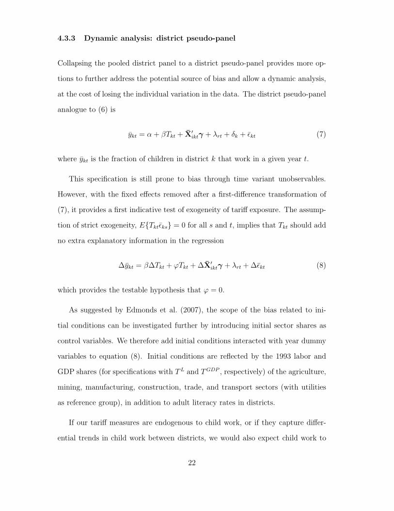
4.3.3 Dynamic analysis: district pseudo-panel
Collapsing the pooled district panel to a district pseudo-panel provides more op-
tions to further address the potential source of bias and allow a dynamic analysis,
at the cost of losing the individual variation in the data. The district pseudo-panel
analogue to (6) is
𝑦𝑘𝑡 = 𝛼 + 𝛽𝑇𝑘𝑡 + X′𝑖𝑘𝑡𝜸 + 𝜆𝑟𝑡 + 𝛿𝑘 + 𝜖𝑘𝑡 (7)
where 𝑦𝑘𝑡 is the fraction of children in district 𝑘 that work in a given year 𝑡.
This specification is still prone to bias through time variant unobservables.
However, with the fixed effects removed after a first-difference transformation of
(7), it provides a first indicative test of exogeneity of tariff exposure. The assump-
tion of strict exogeneity, 𝐸{𝑇𝑘𝑡𝜖𝑘𝑠} = 0 for all 𝑠 and 𝑡, implies that 𝑇𝑘𝑡 should add
no extra explanatory information in the regression
Δ𝑦𝑘𝑡 = 𝛽Δ𝑇𝑘𝑡 + 𝜑𝑇𝑘𝑡 +ΔX′𝑖𝑘𝑡𝜸 + 𝜆𝑟𝑡 +Δ𝜖𝑘𝑡 (8)
which provides the testable hypothesis that 𝜑 = 0.
As suggested by Edmonds et al. (2007), the scope of the bias related to ini-
tial conditions can be investigated further by introducing initial sector shares as
control variables. We therefore add initial conditions interacted with year dummy
variables to equation (8). Initial conditions are reflected by the 1993 labor and
GDP shares (for specifications with 𝑇𝐿 and 𝑇𝐺𝐷𝑃 , respectively) of the agriculture,
mining, manufacturing, construction, trade, and transport sectors (with utilities
as reference group), in addition to adult literacy rates in districts.
If our tariff measures are endogenous to child work, or if they capture differ-
ential trends in child work between districts, we would also expect child work to
22
be correlated with future changes in district tariff exposure. We test this by re-
gressing changes in 𝑦 from 1993 to 1996 on changes in 𝑇 from 1999 to 2002 (i.e.
Δ𝑇𝑘𝑡+2).
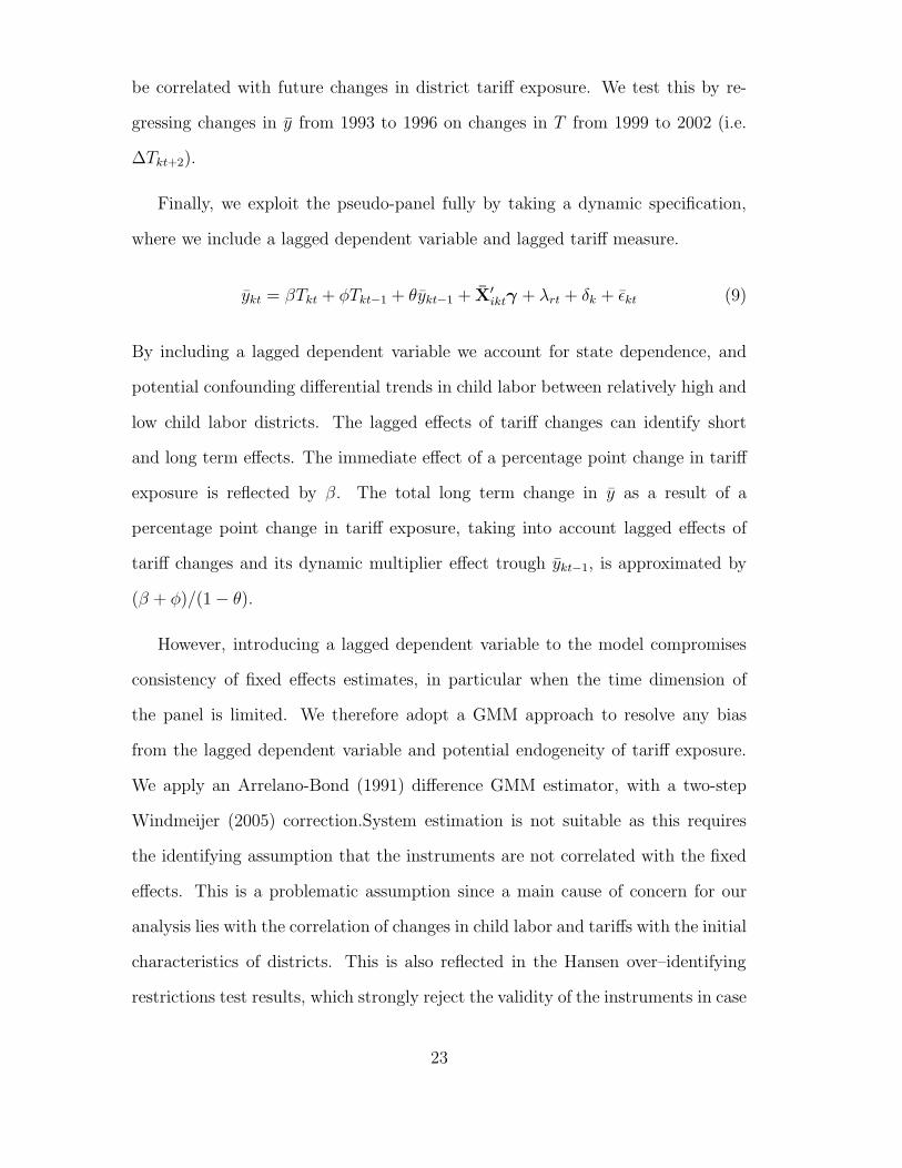
Finally, we exploit the pseudo-panel fully by taking a dynamic specification,
where we include a lagged dependent variable and lagged tariff measure.
𝑦𝑘𝑡 = 𝛽𝑇𝑘𝑡 + 𝜙𝑇𝑘𝑡−1 + 𝜃𝑦𝑘𝑡−1 + X′𝑖𝑘𝑡𝜸 + 𝜆𝑟𝑡 + 𝛿𝑘 + 𝜖𝑘𝑡 (9)
By including a lagged dependent variable we account for state dependence, and
potential confounding differential trends in child labor between relatively high and
low child labor districts. The lagged effects of tariff changes can identify short
and long term effects. The immediate effect of a percentage point change in tariff
exposure is reflected by 𝛽. The total long term change in 𝑦 as a result of a
percentage point change in tariff exposure, taking into account lagged effects of
tariff changes and its dynamic multiplier effect trough 𝑦𝑘𝑡−1, is approximated by
(𝛽 + 𝜙)/(1− 𝜃).
However, introducing a lagged dependent variable to the model compromises
consistency of fixed effects estimates, in particular when the time dimension of
the panel is limited. We therefore adopt a GMM approach to resolve any bias
from the lagged dependent variable and potential endogeneity of tariff exposure.
We apply an Arrelano-Bond (1991) difference GMM estimator, with a two-step
Windmeijer (2005) correction.System estimation is not suitable as this requires
the identifying assumption that the instruments are not correlated with the fixed
effects. This is a problematic assumption since a main cause of concern for our
analysis lies with the correlation of changes in child labor and tariffs with the initial
characteristics of districts. This is also reflected in the Hansen over–identifying
restrictions test results, which strongly reject the validity of the instruments in case
23

of system GMM. We treat tariff exposure and the lagged dependent as endogenous,
and adult literacy as pre-determined. First differences of these variables are then
instrumented with their lagged levels.18
5 Results
5.1 Static analysis
We start by looking at the results from the static analysis, applying specification
(6) to pooled cross section data. The estimated effects of tariff reductions on work
are given in Table 3. The table only reports the coefficients for tariff exposure,
omitting the other covariates for ease of presentation. These include a child’s
age and gender, household size, gender and education of the household head, and
a dummy variable indicating whether a households resides in a rural village or
urbanized precinct within the district.
The basic specification (model A) indicates that a decrease in tariff exposure is
associated with a decrease in child work for 10 to 15 year old children, but the size
of the effect varies between urban and rural areas and also depends on the nature
of the exposure measure. A percentage point decrease in labor weighted tariff
exposure leads to a 1.5 percentage point decrease in work incidence. This result
is mainly driven by the effect in rural districts, where the estimates are larger and
more precise than for municipalities (1.5 and 1.2 percentage points, respectively).
The estimated effects are smaller for GRDP weighted tariff exposure, which would
suggest that tariff changes affect households mainly through labor markets and
less through distributional effects of economic growth.
18 The length of the panel (4 rounds) does not allow us to meaningfully address dynamic effectsthat go beyond one time lag. The number of instruments used in the estimations is 25, 𝑁 is 488for tariffs weighted by GRDP shares and 522 for tariffs weighted by labor shares.
24
Model B investigates differential effects by skill level. The tariff exposure mea-
sure is interacted with the level of education of the head of household, defined as
(i) not completed primary school, (ii) completed primary school, (iii) completed
secondary school and (iv) completed higher education. The benefits of tariff re-
ductions are relatively higher for low skill households.
5.2 Sensitivity analysis and exogeneity tests
The static results are based on district fixed effects, and could be confounding
the effects of trade liberalization and differential growth paths. This section will
examine this potential source of bias.
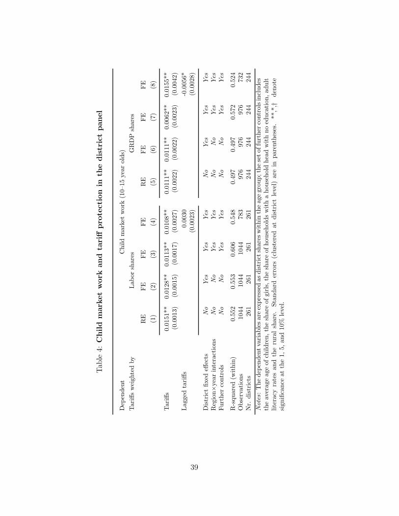
First, the pseudo-panel estimation results for both random and fixed effects
specifications are presented in Table 4. As expected, the correlation between tariff
exposure and the outcome variables is partly driven by time invariant character-
istics of districts and changes in demographics and human capital. In general,
controlling for fixed effects (columns (2) and (6)) reduces the tariff coefficients,
compared to the random effects specification (columns (1) and (5)). Adding co-
variates yields specification (7), and further reduces the effects but improves the
fit (columns (3) and (7)). The effects of tariff changes on child work remain precise
and are consistent with the pooled cross section results, although the coefficients
are slightly smaller.
Simple inclusion of the lagged tariff variable (columns (4) and (8)) indicates
that immediate and longer–term effects of trade liberalization might differ, and
that we may need to consider dynamic effects of tariff changes. While the labor
share weighted results are not sensitive to including a one-period lag of tariff ex-
posure, the GRDP weighted results show an initial large effect which is attenuated
over time.
25

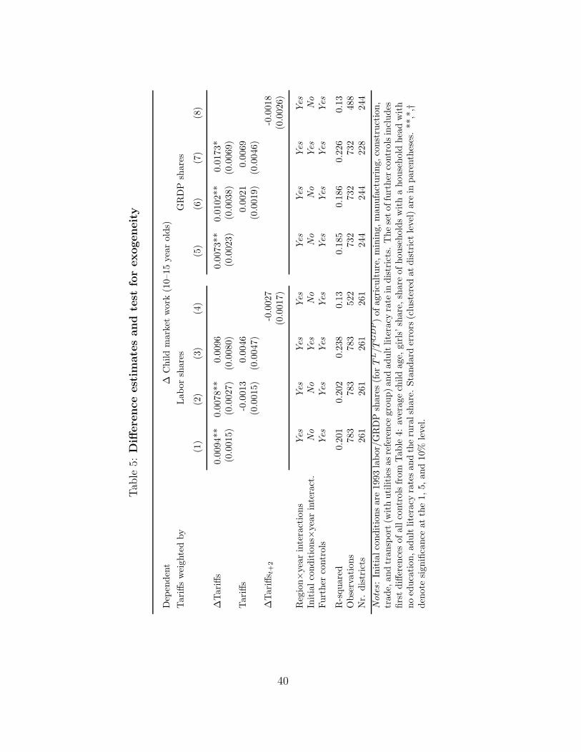
The exogeneity of the tariff measures and sensitivity to initial conditions are
therefore addressed more specifically in Table 5. Columns (1) to (4) show that
the first difference estimates for child work resemble the fixed effects estimates
presented earlier. The tests for strict exogeneity of tariffs exposure with respect to
child work is given in column (2). For both the labor and GRDP weighted tariff
measures the zero hypothesis of strict exogeneity is not rejected. The estimated
effects on child work are also robust to including the initial conditions and year
interaction terms in case of the labor share weighted tariffs (column (3)). The
coefficients increase in size but lose precision when the interaction terms are in-
cluded. Finally, we find no correlation between the two outcome variables and
future tariff changes. The coefficients for two year lead changes in tariff exposure
are small and not statistically significant.
The initial results from the district pseudo panel are fairly robust to specifica-
tion, suggesting that the negative relationship between tariff reduction and child
work is not driven by differential growth trajectories of district economies and
the reduction of the agricultural sector. However, the results also indicate that
the effects of trade liberalization are not static events but are dynamic in nature.
These dynamics are overlooked in a simple fixed effect analysis, which may in fact
capture the confounding result of short– and long–term impacts.
The economic crisis in 1997/98 also raises interpretational concerns, as the
devaluation of the Rupiah resulted in short–term price spikes which affected espe-
cially the poor. Although the effect of the price spike has largely subsided by the
1999 Susenas round, and the overall negative effect of the crisis is controlled for
by the region–time fixed effects included in every regression, concerns still might
remain that the crisis might confound the effects of tariff reductions. This is espe-
cially the case if the effects of the crisis were correlated with the economic structure
26
of the districts. In order to investigate these concerns, Table 6 reports difference
estimates for two separated time periods: 1993–1996 (pre–crisis) and 1999-2002
(post–crisis). The results confirm the robustness of our findings on the effects of
trade liberalization on child labor which are largely unaffected by the split.
5.3 Dynamic analysis
The main GMM estimation results for the dynamic specification are summarized
in Table 7.19 The results are presented by age group, gender and household head
education level.
Decreasing district tariff exposure by one percentage point, leads to a short–
term decrease in child labor incidence of the 10–15 years old by 0.86-1.06 percentage
points depending on which tariff measure we use. Recursive substitution over the
four periods gives us the overall effect of the decrease in local tariff exposure: when
considering labor sector shares, the tariff reductions explain around half (49%) of
the average reduction of child labor of 8.98% points. The overall effect is even
larger when tariff exposure is weighted by district GDP sector shares, explaining
around 70% of the reductions. These figures clearly show that the local effects
of tariff reductions are considerable, but because of the inclusion of region–year
interactions, the magnitudes of these effects cannot be interpreted directly.
Reduction in child work due to tariff reductions are strongest in the age group
of 13 to 15 years old, which is not surprising given the low incidence of child work
among primary school age children. We do not see a gender gap, as the effects are
19 The full specification and detailed results are reported in the supplemental appendix, Table11. Note that the Hansen over–identification test rejects the validity of the instruments at 10percent level for the urban child work estimates. The Hansen test also rejects at 10 percent levelfor some of the sub-samples, in particular the youngest age group, boys and households withno educated head of household. Hence, these results need to be interpreted with some caution,although the previous analysis shows little evidence of endogeneity of tariff exposure with respectto child work.
27

of comparable size for both girls and boys. When we consider tariff exposure based
on district labor shares, improvements in child labor are irrespective of household
skill composition, while children from relatively low skill households seem to be
the main beneficiaries of trade liberalization based on the GDP sector shares of the
local economy. When decomposing these effects for the rural and urban subsamples
(cf. Table 8), it becomes apparent that these favorable effects are mainly rural,
irrespective of the tariff weighting scheme.
Our study remains largely a reduced form analysis, and we are not able to
identify the main transmission channels through which child work is affected by
reduced tariff exposure. Nevertheless, we can provide some global indication of
the main mechanisms at work, by looking at the effects on district poverty profiles
and adult employment.
Tariff reductions have lead to a reduction in the extent and severity of poverty.
Table 9 shows the estimated effects of reduced tariff exposure on the poverty
head count ratio (Panel A) and the squared poverty gap (Panel B), where the
model specification is similar to the earlier dynamic GMM. While the poverty head
count merely records the fraction of the district population that cross an arbitrary
level of consumption, the squared poverty gap reflects the curvature in the per
capita expenditure distribution for the population living below the poverty line.
The results show that a percentage point reduction in tariff exposure reduces the
poverty headcount in districts by 1.2 percentage points, and also reduces inequality
among the poor. In other words, the results seem to suggest that income effects
play a role, in particular at the bottom end of the income distribution.
Tariff reductions do not impact workforce participation of cohorts older than 18
(cf. results in Table 10). This would suggest that the effect of trade liberalization
on child labor is not driven by substitution of child for adult labor, and that the
28
observed income effects are not due to a labor supply response and reduced unem-
ployment. Rather, income effects seem to be a result of relative wage increases, in
particular for low skill labor.
6 Conclusion
This paper examined the effects of trade liberalization on child work in Indonesia.
In the 1990s, Indonesia went through a major reduction in tariff barriers, as average
import tariff lines decreased from around 17.2 percent in 1993 to 6.6 percent in
2002; a period which also saw reductions in child work.
We identify the effects of trade liberalization by combining geographic varia-
tion in sector composition of the economy with temporal variation in tariff lines
by product category. This yields geographic variation in changes in average expo-
sure to trade liberalization over time, hence identifying geographical differences in
the effects of trade policy. The results are robust to specification and sensitivity
analysis, and we find no evidence of remaing sources of bias.
Our main findings suggest that Indonesia’s trade liberalization experience in
the 1990s has contributed to a strong decline in child labor, as decreased tariff
exposure is associated with a decrease in work by 10 to 15 year old children. The
effects of tariff reductions increase with the age of children, and are strongest for
children from low skill backgrounds and in rural areas. Through these effects,
trade liberalization will have long term welfare implications for human capital
investments, in particular for low skill, and presumably poorer, households.
Although our reduced form analysis can at best provide indirect evidence of
the main transmission channels, we do find strong support for the hypothesis that
reduction of child labor is driven by positive income effects from trade liberalization
29
for the poorest. This is consistent with other studies, which argue that trade
liberalization in Indonesia brought about a relative wage increase for low skill
labor, although causal effects are hard to confirm (Suryahadi 2001, Arnold and
Smarzynska Javorcik 2005, Sitalaksmi et al. 2007). Further analysis of this causal
relationship would be an area of future research.
The mixed empirical evidence from this paper and other country studies would
suggest that the potential benefits to be gained from trade liberalization, and its
distributional implications, are indeed context specific. The Indonesian context
seems to have provided the pre–conditions needed to generate classic Stolper–
Samuelson effects, partly facilitated by a coinciding process of structural change
in the 1990s that saw a reallocation of labor from agriculture to services and
manufacturing. In particular the mobility of low skill labor seems to play an
important role, which, combined with increased productivity and competitiveness,
has lead to better employment opportunities outside agriculture and increased
returns to low skill labor. Such cross–country heterogeneinty may be underlying
the weak average effects of trade liberalization on child labor and human capital
investments found at macro level, highlighting the importance of considering local
economic contexts when propagating trade reforms and formulating subsequent
social policy responses.
30
References
Amiti, M. and Konings, J.: 2007, Trade liberalization, intermediate inputs and pro-
ductivity: Evidence from Indonesia, American Economic Review 97(5), 1611–
1638.
Arellano, M. and Bond, S.: 1991, Some tests of specification for panel data: Monte
Carlo evidence and an application to employment equations, Review of Eco-
nomic Studies 58(2), 277–297.
Arnold, J. and Smarzynska Javorcik, B.: 2005, Gifted kids or pushy parents?
Foreign acquisitions and plant performance in Indonesia, CEPR Discussion
Papers 5065, C.E.P.R.
Basri, M. C. and Hill, H.: 2004, Ideas, interests and oil prices: The political
economy of trade reform during Soeharto’s Indonesia, The World Economy
27(5), 633–655.
Basu, K. and Van, P. H.: 1998, The economics of child labor, American Economic
Review 88(3), 412–427.
Beegle, K., Dehejia, R. H. and Gatti, R.: 2006, Child labor and agricultural shocks,
Journal of Development Economics 81(1), 80–96.
Bhagwati, J. and Srinivasan, T. N.: 2002, Trade and poverty in the poor countries,
American Economic Review 92(2), 180–183.
Cameron, L. A.: 2001, The impact of the Indonesian financial crisis on children:
An analysis using the 100 villages survey, Bulletin of Indonesian Economic
Studies 37(1), 43–64.
31
Cigno, A., Rosati, F. C. and Guarcello, L.: 2002, Does globalisation increase child
labour?, World Development 30(9), 1579–1589.
Davis, D. R. and Mishra, P.: 2007, Stolper-Samuelson is dead: And other crimes of
both theory and data, in A. Harrison (ed.), Globalization and Poverty, NBER
Chapters, National Bureau of Economic Research, Inc, pp. 87–108.
Edmonds, E. V. and Pavcnik, N.: 2005a, Child labor in a global economy, Journal
of Economic Perspectives 8(1), 199–220.
Edmonds, E. V. and Pavcnik, N.: 2005b, The effect of trade liberalization on child
labor, Journal of International Economics 65(2), 401–419.
Edmonds, E. V. and Pavcnik, N.: 2006, International trade and child labor: Cross–
country evidence, Journal of International Economics 68(1), 115–140.
Edmonds, E. V., Pavcnik, N. and Topalova, P.: 2007, Trade adjustment and hu-
man capital investments: Evidence from Indian tariff reform, NBER Working
Papers 12884, National Bureau of Economic Research, Inc.
Fane, G.: 1999, Indonesian economic policies and performance, 1960-98, The
World Economy 22(5), 651–668.
Harrison, A.: 2007, Globalization and Poverty, NBER Books, University of
Chicago Press for NBER.
Hertel, T. W., Ivanic, M., Preckel, P. V. and Cranfield, J. A. L.: 2004, The
earnings effects of multilateral trade liberalization: Implications for poverty,
The World Bank Economic Review 18(2), 205–236.
Hill, H., Resosudarmo, B. P. and Vidyattama, Y.: 2008, Indonesia’s changing
economic geography, Bulletin of Indonesian Economic Studies 44(3), 407–
435.
32
Jafarey, S. and Lahiri, S.: 2002, Will trade sanctions reduce child labour?, Journal
of Development Economics 68(1), 137–156.
Jones, G. W. and Hagul, P.: 2001, Schooling in Indonesia: Crisis-related and
longer-term issues, Bulletin of Indonesian Economic Studies 37(2), 207–231.
Kis-Katos, K.: 2007, Does globalization reduce child labor?, Journal of Interna-
tional Trade and Economic Development 16(1), 71–92.
Kis-Katos, K. and Schulze, G.: 2009, Child labor in Indonesian small industries,
Discussion Paper Series 10, University of Freiburg, Department of Interna-
tional Economic Policy.
Komiya, R.: 1967, Non-traded goods and the pure theory of international trade,
International Economic Review 8(2), 132–152.
Lanjouw, P., Pradhan, M., Saadah, F., Sayed, H. and Sparrow, R.: 2002, Poverty,
education and health in Indonesia: Who benefits from public spending?, in
C. Morrisson (ed.), Education and Health Expenditures, and Development:
The cases of Indonesia and Peru, OECD Development Centre, Paris, pp. 17–
78.
Manning, C.: 2000, The economic crisis and child labor in Indonesia, ILO/IPEC
Working Paper, International Labour Office, Geneva.
Paqueo, V. and Sparrow, R.: 2006, Free basic education in Indonesia: Policy
scenarios and implications for school enrolment, Mimeo, The World Bank,
Jakarta.
Pradhan, M., Suryahadi, A., Sumarto, S. and Pritchett, L.: 2001, Eating like which
“Joneses?” An iterative solution to the choice of a poverty line “reference
group”, Review of Income and Wealth 47(4), 473–487.
33
Ranjan, P.: 2001, Credit constraints and the phenomenon of child labor, Journal
of Development Economics 64(1), 81–102.
Sitalaksmi, S., Ismalina, P., Fitrady, A. and Robertson, R.: 2007, Globalization
and working conditions: Evidence from Indonesia, Technical report, mimeo.
Suryahadi, A.: 2001, International economic integration and labor markets: The
case of Indonesia, Economics Study Area Working Papers 22, East-West Cen-
ter, Economics Study Area.
Suryahadi, A., Priyambada, A. and Sumarto, S.: 2005, Poverty, school and work:
Children during the economic crisis in Indonesia, Development and Change
36(2), 351–373.
Suryahadi, A., Sumarto, S. and Pritchett, L.: 2003, Evolution of poverty during
the crisis in Indonesia, Asian Economic Journal 17(3), 221–241.
Suryahadi, A., Suryadarma, D. and Sumarto, S.: 2009, The effects of location and
sectoral components of economic growth on poverty: Evidence from Indone-
sia, Journal of Development Economics 89(1), 109–117.
Topalova, P.: 2005, Trade liberalization, poverty, and inequality: Evidence from
Indian districts, NBER Working Papers 11614, National Bureau of Economic
Research, Inc.
Windmeijer, F.: 2005, A finite sample correction for the variance of linear efficient
two-step GMM estimators, Journal of Econometrics 126(1), 25–51.
World Bank: 2006, Making Indonesia Work for the Poor, World Bank Office
Jakarta.
WTO: 1998, Trade Policy Review Indonesia, Geneva.
34

WTO: 2003, Trade Policy Review Indonesia, Geneva.
35
A Tables
Table 1: Evolution of market work of children over time
Share of boys aged 10–15 doing market work
By head’s educational attainment By districtYear None Primary Low sec. Higher Rural Urban Total 𝑁
1993 0.247 0.159 0.086 0.037 0.197 0.044 0.174 63,0091994 0.232 0.139 0.072 0.041 0.176 0.043 0.156 63,5561995 0.236 0.139 0.078 0.037 0.180 0.050 0.161 59,9921996 0.202 0.124 0.073 0.036 0.153 0.045 0.137 61,2341997 0.179 0.107 0.054 0.029 0.129 0.028 0.115 58,4871998 0.197 0.122 0.082 0.033 0.144 0.048 0.130 56,7831999 0.178 0.111 0.065 0.030 0.130 0.040 0.117 54,9072000 0.150 0.092 0.052 0.024 0.106 0.026 0.096 51,0032001 0.173 0.107 0.070 0.031 0.124 0.036 0.112 56,3792002 0.140 0.080 0.046 0.021 0.090 0.030 0.082 56,243
𝑁 222,837 191,241 67,801 99,714 477,500 104,093 581,593 581,593
Share of girls aged 10–15 doing market work
By head’s educational attainment By districtYear None Primary Low sec. Higher Rural Urban Total 𝑁
1993 0.177 0.113 0.080 0.069 0.143 0.067 0.131 59,8951994 0.169 0.103 0.060 0.064 0.128 0.066 0.119 59,5821995 0.152 0.102 0.072 0.066 0.125 0.064 0.115 57,1021996 0.137 0.085 0.058 0.053 0.106 0.052 0.098 58,4301997 0.109 0.067 0.046 0.043 0.082 0.037 0.075 55,4271998 0.127 0.084 0.060 0.050 0.097 0.060 0.091 53,8141999 0.120 0.068 0.051 0.045 0.087 0.044 0.080 51,9362000 0.094 0.061 0.041 0.030 0.070 0.030 0.065 47,8322001 0.109 0.070 0.053 0.043 0.081 0.047 0.076 52,9382002 0.092 0.049 0.032 0.029 0.059 0.037 0.056 52,752
𝑁 207,841 180,188 64,162 97,517 447,531 102,177 549,708 549,708
Notes : Participation shares are weighted by survey weights. 𝑁 refers to the numberof observations in the sample, rural districts denote Kabupatens, urban districts denoteKotas.
36
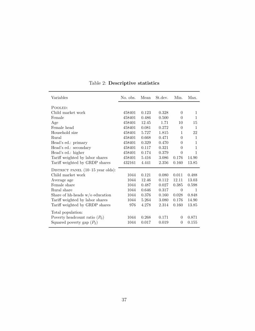
Table 2: Descriptive statistics
Variables No. obs. Mean St.dev. Min. Max.
Pooled:Child market work 458401 0.123 0.328 0 1Female 458401 0.486 0.500 0 1Age 458401 12.45 1.71 10 15Female head 458401 0.081 0.272 0 1Household size 458401 5.727 1.815 1 22Rural 458401 0.668 0.471 0 1Head’s ed.: primary 458401 0.329 0.470 0 1Head’s ed.: secondary 458401 0.117 0.321 0 1Head’s ed.: higher 458401 0.174 0.379 0 1Tariff weighted by labor shares 458401 5.416 3.086 0.176 14.90Tariff weighted by GRDP shares 432161 4.441 2.356 0.160 13.85
District panel (10–15 year olds):Child market work 1044 0.121 0.080 0.011 0.488Average age 1044 12.46 0.112 12.11 13.03Female share 1044 0.487 0.027 0.385 0.598Rural share 1044 0.646 0.317 0 1Share of hh-heads w/o education 1044 0.376 0.160 0.028 0.848Tariff weighted by labor shares 1044 5.264 3.080 0.176 14.90Tariff weighted by GRDP shares 976 4.278 2.314 0.160 13.85
Total population:Poverty headcount ratio (𝑃0) 1044 0.268 0.171 0 0.871Squared poverty gap (𝑃2) 1044 0.017 0.019 0 0.155
37
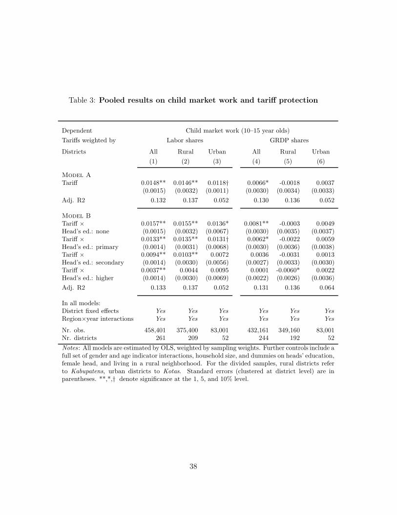
Table 3: Pooled results on child market work and tariff protection
Dependent Child market work (10–15 year olds)
Tariffs weighted by Labor shares GRDP shares
Districts All Rural Urban All Rural Urban
(1) (2) (3) (4) (5) (6)
Model ATariff 0.0148** 0.0146** 0.0118† 0.0066* -0.0018 0.0037
(0.0015) (0.0032) (0.0011) (0.0030) (0.0034) (0.0033)
Adj. R2 0.132 0.137 0.052 0.130 0.136 0.052
Model BTariff × 0.0157** 0.0155** 0.0136* 0.0081** -0.0003 0.0049Head’s ed.: none (0.0015) (0.0032) (0.0067) (0.0030) (0.0035) (0.0037)Tariff × 0.0133** 0.0135** 0.0131† 0.0062* -0.0022 0.0059Head’s ed.: primary (0.0014) (0.0031) (0.0068) (0.0030) (0.0036) (0.0038)Tariff × 0.0094** 0.0103** 0.0072 0.0036 -0.0031 0.0013Head’s ed.: secondary (0.0014) (0.0030) (0.0056) (0.0027) (0.0033) (0.0030)Tariff × 0.0037** 0.0044 0.0095 0.0001 -0.0060* 0.0022Head’s ed.: higher (0.0014) (0.0030) (0.0069) (0.0022) (0.0026) (0.0036)
Adj. R2 0.133 0.137 0.052 0.131 0.136 0.064
In all models:District fixed effects Yes Yes Yes Yes Yes YesRegion×year interactions Yes Yes Yes Yes Yes Yes
Nr. obs. 458,401 375,400 83,001 432,161 349,160 83,001Nr. districts 261 209 52 244 192 52
Notes : All models are estimated by OLS, weighted by sampling weights. Further controls include afull set of gender and age indicator interactions, household size, and dummies on heads’ education,female head, and living in a rural neighborhood. For the divided samples, rural districts referto Kabupatens, urban districts to Kotas. Standard errors (clustered at district level) are inparentheses. **,*,† denote significance at the 1, 5, and 10% level.
38
Tab
le4:Childmarketwork
andtariffprotectionin
thedistrictpanel
Dep
enden
tC
hild
mark
etw
ork
(10–15
yea
rold
s)
Tari
ffs
wei
ghte
dby
Labor
share
sG
RD
Psh
are
s
RE
FE
FE
FE
RE
FE
FE
FE
(1)
(2)
(3)
(4)
(5)
(6)
(7)
(8)
Tari
ffs
0.0
151**
0.0
128**
0.0
113**
0.0
108**
0.0
111**
0.0
111**
0.0
062**
0.0
155**
(0.0
013)
(0.0
015)
(0.0
017)
(0.0
027)
(0.0
022)
(0.0
022)
(0.0
023)
(0.0
042)
Lagged
tari
ffs
0.0
030
-0.0
056*
(0.0
023)
(0.0
028)
Dis
tric
tfixed
effec
tsNo
Yes
Yes
Yes
No
Yes
Yes
Yes
Reg
ion×y
ear
inte
ract
ions
No
No
Yes
Yes
No
No
Yes
Yes
Furt
her
contr
ols
No
No
Yes
Yes
No
No
Yes
Yes
R-s
quare
d(w
ithin
)0.5
52
0.5
53
0.6
06
0.5
48
0.4
97
0.4
97
0.5
72
0.5
24
Obse
rvations
1044
1044
1044
783
976
976
976
732
Nr.
dis
tric
ts261
261
261
261
244
244
244
244
Notes:
The
dep
enden
tva
riable
sare
expre
ssed
asdis
tric
tsh
are
sw
ithin
the
agegro
up;th
ese
toffu
rther
contr
ols
incl
udes
the
aver
age
age
ofch
ildre
n,th
esh
are
ofgir
ls,th
esh
are
ofhouse
hold
sw
ith
ahouse
hold
hea
dw
ith
no
educa
tion,adult
lite
racy
rate
sand
the
rura
lsh
are
.Sta
ndard
erro
rs(c
lust
ered
at
dis
tric
tle
vel
)are
inpare
nth
eses
.**,*
,†den
ote
signifi
cance
at
the
1,5,and
10%
level
.
39
Tab
le5:Difference
estimatesandtestforexogeneity
Dep
enden
tΔ
Child
mark
etw
ork
(10–15
yea
rold
s)
Tari
ffs
wei
ghte
dby
Labor
share
sG
RD
Psh
are
s
(1)
(2)
(3)
(4)
(5)
(6)
(7)
(8)
ΔTari
ffs
0.0
094**
0.0
078**
0.0
096
0.0
073**
0.0
102**
0.0
173*
(0.0
015)
(0.0
027)
(0.0
080)
(0.0
023)
(0.0
038)
(0.0
069)
Tari
ffs
-0.0
013
0.0
046
0.0
021
0.0
069
(0.0
015)
(0.0
047)
(0.0
019)
(0.0
046)
ΔTari
ffs 𝑡+2
-0.0
027
-0.0
018
(0.0
017)
(0.0
026)
Reg
ion×y
ear
inte
ract
ions
Yes
Yes
Yes
Yes
Yes
Yes
Yes
Yes
Initia
lco
nditio
ns×
yea
rin
tera
ct.
No
No
Yes
No
No
No
Yes
No
Furt
her
contr
ols
Yes
Yes
Yes
Yes
Yes
Yes
Yes
Yes
R-s
quare
d0.2
01
0.2
02
0.2
38
0.1
30.1
85
0.1
86
0.2
26
0.1
3O
bse
rvations
783
783
783
522
732
732
732
488
Nr.
dis
tric
ts261
261
261
261
244
244
228
244
Notes:
Initia
lco
nditio
ns
are
1993
labor/
GR
DP
share
s(f
or𝑇
𝐿/𝑇
𝐺𝐷𝑃)
ofagri
culture
,m
inin
g,m
anufa
cturi
ng,co
nst
ruct
ion,
trade,
and
transp
ort
(with
utilities
asre
fere
nce
gro
up)and
adult
lite
racy
rate
indis
tric
ts.
The
setoffu
rther
contr
ols
incl
udes
firs
tdiff
eren
ces
ofall
contr
ols
from
Table
4:
aver
age
child
age,
gir
ls’sh
are
,sh
are
ofhouse
hold
sw
ith
ahouse
hold
hea
dw
ith
no
educa
tion,adult
lite
racy
rate
sand
the
rura
lsh
are
.Sta
ndard
erro
rs(c
lust
ered
atdis
tric
tle
vel
)are
inpare
nth
eses
.**,*
,†den
ote
signifi
cance
at
the
1,5,and
10%
level
.
40
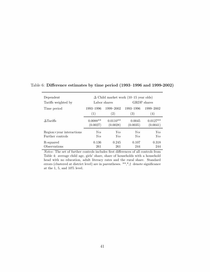
Table 6: Difference estimates by time period (1993–1996 and 1999-2002)
Dependent Δ Child market work (10–15 year olds)
Tariffs weighted by Labor shares GRDP shares
Time period 1993–1996 1999–2002 1993–1996 1999–2002
(1) (2) (3) (4)
ΔTariffs 0.0088** 0.0110** 0.0045 0.0127**(0.0027) (0.0028) (0.0035) (0.0041)
Region×year interactions Yes Yes Yes YesFurther controls Yes Yes Yes Yes
R-squared 0.136 0.245 0.107 0.318Observations 261 261 244 244
Notes : The set of further controls includes first differences of all controls fromTable 4: average child age, girls’ share, share of households with a householdhead with no education, adult literacy rates and the rural share. Standarderrors (clustered at district level) are in parentheses. **,*,† denote significanceat the 1, 5, and 10% level.
41
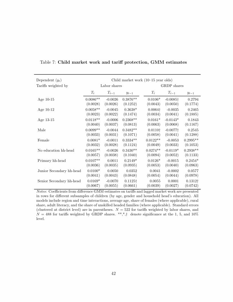
Table 7: Child market work and tariff protection, GMM estimates
Dependent (𝑦𝑡) Child market work (10–15 year olds)
Tariffs weighted by Labor shares GRDP shares
𝑇𝑡 𝑇𝑡−1 𝑦𝑡−1 𝑇𝑡 𝑇𝑡−1 𝑦𝑡−1
Age 10-15 0.0086** -0.0026 0.3876** 0.0106* -0.0085† 0.2794(0.0028) (0.0026) (0.1252) (0.0043) (0.0050) (0.1774)
Age 10-12 0.0058** -0.0045 0.3638* 0.0064† -0.0035 0.2465(0.0023) (0.0022) (0.1474) (0.0034) (0.0041) (0.1885)
Age 13-15 0.0118** -0.0006 0.2368** 0.0161* -0.0143* 0.1843(0.0040) (0.0037) (0.0813) (0.0063) (0.0068) (0.1167)
Male 0.0099** -0.0044 0.3482** 0.0110† -0.0077† 0.2545(0.0033) (0.0031) (0.1071) (0.0058) (0.0041) (0.1288)
Female 0.0081* -0.0011 0.3334** 0.0122** -0.0053 0.2995**(0.0032) (0.0028) (0.1124) (0.0049) (0.0033) (0.1053)
No education hh-head 0.0165** -0.0026 0.3430** 0.0274** -0.0119* 0.2938**(0.0057) (0.0038) (0.1040) (0.0094) (0.0052) (0.1133)
Primary hh-head 0.0107** 0.0011 0.2149* 0.0126* -0.0015 0.2454*(0.0036) (0.0035) (0.0935) (0.0053) (0.0040) (0.0963)
Junior Secondary hh-head 0.0100* 0.0050 0.0352 0.0041 -0.0002 0.0577(0.0041) (0.0043) (0.0848) (0.0054) (0.0044) (0.0978)
Senior Secondary hh-head 0.0169* -0.0070 0.1125† 0.0055 0.0001 0.1312†(0.0067) (0.0055) (0.0661) (0.0039) (0.0027) (0.0742)
Notes : Coefficients from difference GMM estimates on tariffs and lagged market work are presentedin rows for different subsamples of children (by age, gender and household head’s education). Allmodels include region and time interactions, average age, share of females (where applicable), ruralshare, adult literacy, and the share of unskilled headed families (where applicable). Standard errors(clustered at district level) are in parentheses. 𝑁 = 522 for tariffs weighted by labor shares, and𝑁 = 488 for tariffs weighted by GRDP shares. **,*,† denote significance at the 1, 5, and 10%level.
42
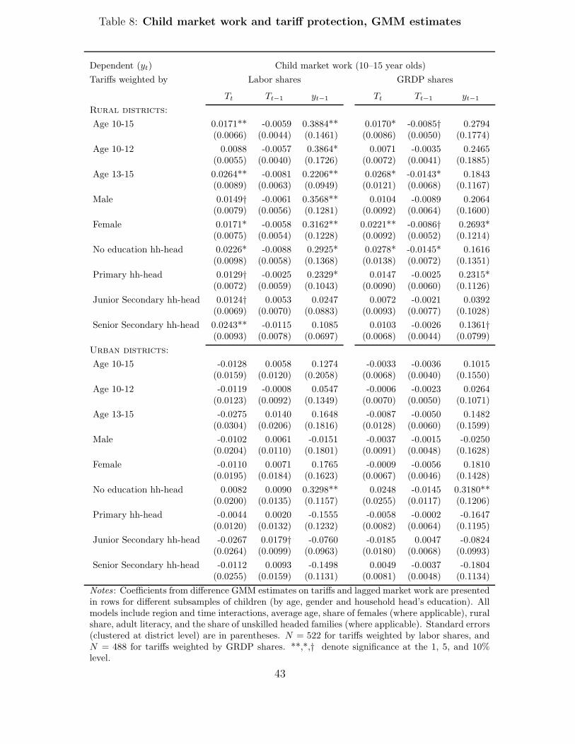
Table 8: Child market work and tariff protection, GMM estimates
Dependent (𝑦𝑡) Child market work (10–15 year olds)
Tariffs weighted by Labor shares GRDP shares
𝑇𝑡 𝑇𝑡−1 𝑦𝑡−1 𝑇𝑡 𝑇𝑡−1 𝑦𝑡−1
Rural districts:
Age 10-15 0.0171** -0.0059 0.3884** 0.0170* -0.0085† 0.2794(0.0066) (0.0044) (0.1461) (0.0086) (0.0050) (0.1774)
Age 10-12 0.0088 -0.0057 0.3864* 0.0071 -0.0035 0.2465(0.0055) (0.0040) (0.1726) (0.0072) (0.0041) (0.1885)
Age 13-15 0.0264** -0.0081 0.2206** 0.0268* -0.0143* 0.1843(0.0089) (0.0063) (0.0949) (0.0121) (0.0068) (0.1167)
Male 0.0149† -0.0061 0.3568** 0.0104 -0.0089 0.2064(0.0079) (0.0056) (0.1281) (0.0092) (0.0064) (0.1600)
Female 0.0171* -0.0058 0.3162** 0.0221** -0.0086† 0.2693*(0.0075) (0.0054) (0.1228) (0.0092) (0.0052) (0.1214)
No education hh-head 0.0226* -0.0088 0.2925* 0.0278* -0.0145* 0.1616(0.0098) (0.0058) (0.1368) (0.0138) (0.0072) (0.1351)
Primary hh-head 0.0129† -0.0025 0.2329* 0.0147 -0.0025 0.2315*(0.0072) (0.0059) (0.1043) (0.0090) (0.0060) (0.1126)
Junior Secondary hh-head 0.0124† 0.0053 0.0247 0.0072 -0.0021 0.0392(0.0069) (0.0070) (0.0883) (0.0093) (0.0077) (0.1028)
Senior Secondary hh-head 0.0243** -0.0115 0.1085 0.0103 -0.0026 0.1361†(0.0093) (0.0078) (0.0697) (0.0068) (0.0044) (0.0799)
Urban districts:
Age 10-15 -0.0128 0.0058 0.1274 -0.0033 -0.0036 0.1015(0.0159) (0.0120) (0.2058) (0.0068) (0.0040) (0.1550)
Age 10-12 -0.0119 -0.0008 0.0547 -0.0006 -0.0023 0.0264(0.0123) (0.0092) (0.1349) (0.0070) (0.0050) (0.1071)
Age 13-15 -0.0275 0.0140 0.1648 -0.0087 -0.0050 0.1482(0.0304) (0.0206) (0.1816) (0.0128) (0.0060) (0.1599)
Male -0.0102 0.0061 -0.0151 -0.0037 -0.0015 -0.0250(0.0204) (0.0110) (0.1801) (0.0091) (0.0048) (0.1628)
Female -0.0110 0.0071 0.1765 -0.0009 -0.0056 0.1810(0.0195) (0.0184) (0.1623) (0.0067) (0.0046) (0.1428)
No education hh-head 0.0082 0.0090 0.3298** 0.0248 -0.0145 0.3180**(0.0200) (0.0135) (0.1157) (0.0255) (0.0117) (0.1206)
Primary hh-head -0.0044 0.0020 -0.1555 -0.0058 -0.0002 -0.1647(0.0120) (0.0132) (0.1232) (0.0082) (0.0064) (0.1195)
Junior Secondary hh-head -0.0267 0.0179† -0.0760 -0.0185 0.0047 -0.0824(0.0264) (0.0099) (0.0963) (0.0180) (0.0068) (0.0993)
Senior Secondary hh-head -0.0112 0.0093 -0.1498 0.0049 -0.0037 -0.1804(0.0255) (0.0159) (0.1131) (0.0081) (0.0048) (0.1134)
Notes : Coefficients from difference GMM estimates on tariffs and lagged market work are presentedin rows for different subsamples of children (by age, gender and household head’s education). Allmodels include region and time interactions, average age, share of females (where applicable), ruralshare, adult literacy, and the share of unskilled headed families (where applicable). Standard errors(clustered at district level) are in parentheses. 𝑁 = 522 for tariffs weighted by labor shares, and𝑁 = 488 for tariffs weighted by GRDP shares. **,*,† denote significance at the 1, 5, and 10%level.
43
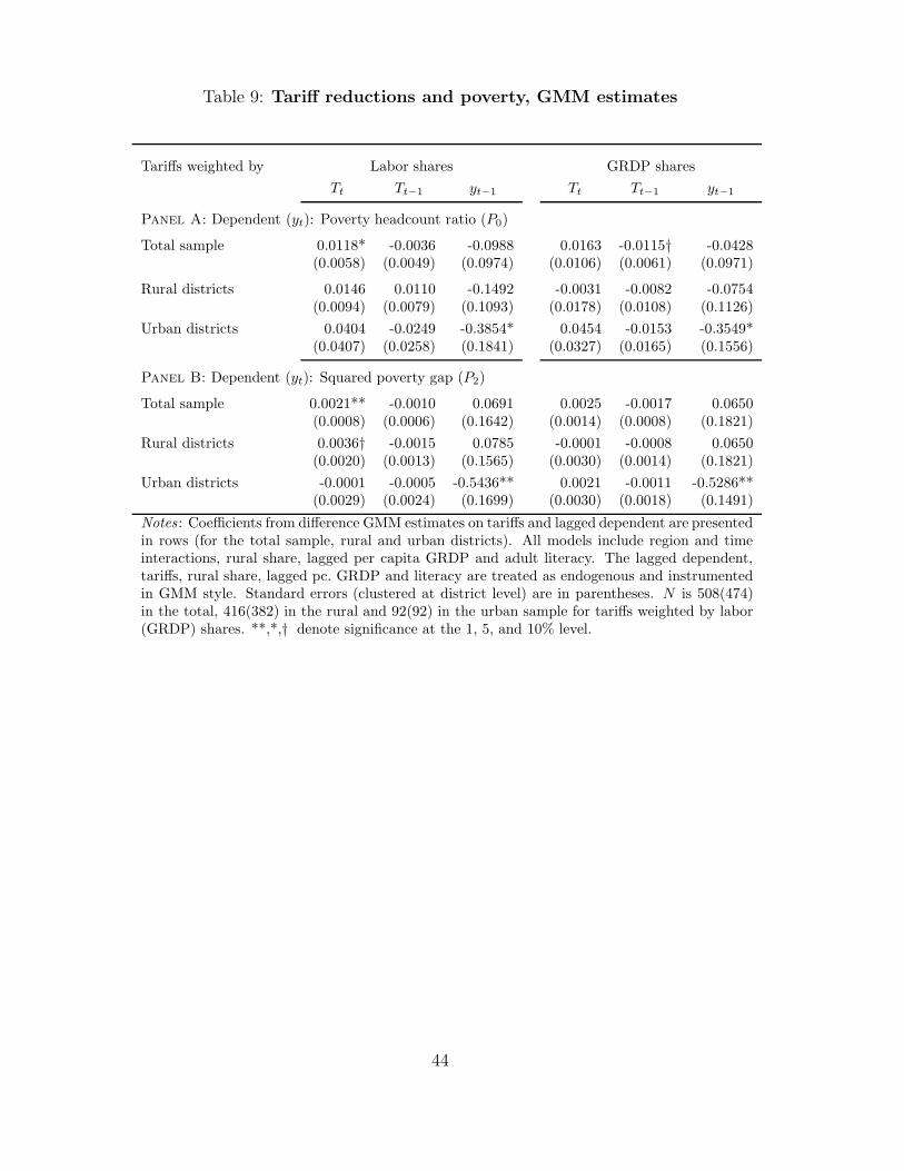
Table 9: Tariff reductions and poverty, GMM estimates
Tariffs weighted by Labor shares GRDP shares
𝑇𝑡 𝑇𝑡−1 𝑦𝑡−1 𝑇𝑡 𝑇𝑡−1 𝑦𝑡−1
Panel A: Dependent (𝑦𝑡): Poverty headcount ratio (𝑃0)
Total sample 0.0118* -0.0036 -0.0988 0.0163 -0.0115† -0.0428(0.0058) (0.0049) (0.0974) (0.0106) (0.0061) (0.0971)
Rural districts 0.0146 0.0110 -0.1492 -0.0031 -0.0082 -0.0754(0.0094) (0.0079) (0.1093) (0.0178) (0.0108) (0.1126)
Urban districts 0.0404 -0.0249 -0.3854* 0.0454 -0.0153 -0.3549*(0.0407) (0.0258) (0.1841) (0.0327) (0.0165) (0.1556)
Panel B: Dependent (𝑦𝑡): Squared poverty gap (𝑃2)
Total sample 0.0021** -0.0010 0.0691 0.0025 -0.0017 0.0650(0.0008) (0.0006) (0.1642) (0.0014) (0.0008) (0.1821)
Rural districts 0.0036† -0.0015 0.0785 -0.0001 -0.0008 0.0650(0.0020) (0.0013) (0.1565) (0.0030) (0.0014) (0.1821)
Urban districts -0.0001 -0.0005 -0.5436** 0.0021 -0.0011 -0.5286**(0.0029) (0.0024) (0.1699) (0.0030) (0.0018) (0.1491)
Notes : Coefficients from difference GMM estimates on tariffs and lagged dependent are presentedin rows (for the total sample, rural and urban districts). All models include region and timeinteractions, rural share, lagged per capita GRDP and adult literacy. The lagged dependent,tariffs, rural share, lagged pc. GRDP and literacy are treated as endogenous and instrumentedin GMM style. Standard errors (clustered at district level) are in parentheses. 𝑁 is 508(474)in the total, 416(382) in the rural and 92(92) in the urban sample for tariffs weighted by labor(GRDP) shares. **,*,† denote significance at the 1, 5, and 10% level.
44
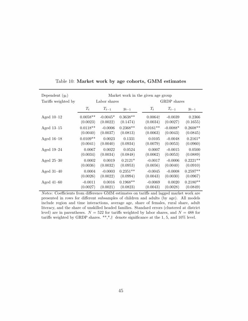
Table 10: Market work by age cohorts, GMM estimates
Dependent (𝑦𝑡) Market work in the given age group
Tariffs weighted by Labor shares GRDP shares
𝑇𝑡 𝑇𝑡−1 𝑦𝑡−1 𝑇𝑡 𝑇𝑡−1 𝑦𝑡−1
Aged 10–12 0.0058** -0.0045* 0.3638** 0.0064† -0.0039 0.2366(0.0023) (0.0022) (0.1474) (0.0034) (0.0027) (0.1655)
Aged 13–15 0.0118** -0.0006 0.2368** 0.0161** -0.0088* 0.2608**(0.0040) (0.0037) (0.0813) (0.0063) (0.0043) (0.0845)
Aged 16–18 0.0109** 0.0023 0.1331 0.0105 -0.0048 0.2161*(0.0041) (0.0040) (0.0934) (0.0079) (0.0053) (0.0960)
Aged 19–24 0.0067 0.0022 0.0524 0.0007 -0.0015 0.0500(0.0034) (0.0034) (0.0848) (0.0062) (0.0053) (0.0889)
Aged 25–30 0.0002 0.0019 0.2121* -0.0017 -0.0006 0.2221**(0.0036) (0.0032) (0.0953) (0.0056) (0.0040) (0.0910)
Aged 31–40 0.0004 -0.0003 0.2351** -0.0045 -0.0008 0.2597**(0.0026) (0.0022) (0.0994) (0.0043) (0.0030) (0.0967)
Aged 41–60 -0.0011 0.0016 0.1968** -0.0069 0.0020 0.2180**(0.0027) (0.0021) (0.0823) (0.0043) (0.0028) (0.0849)
Notes : Coefficients from difference GMM estimates on tariffs and lagged market work arepresented in rows for different subsamples of children and adults (by age). All modelsinclude region and time interactions, average age, share of females, rural share, adultliteracy, and the share of unskilled headed families. Standard errors (clustered at districtlevel) are in parentheses. 𝑁 = 522 for tariffs weighted by labor shares, and 𝑁 = 488 fortariffs weighted by GRDP shares. **,*,† denote significance at the 1, 5, and 10% level.
45
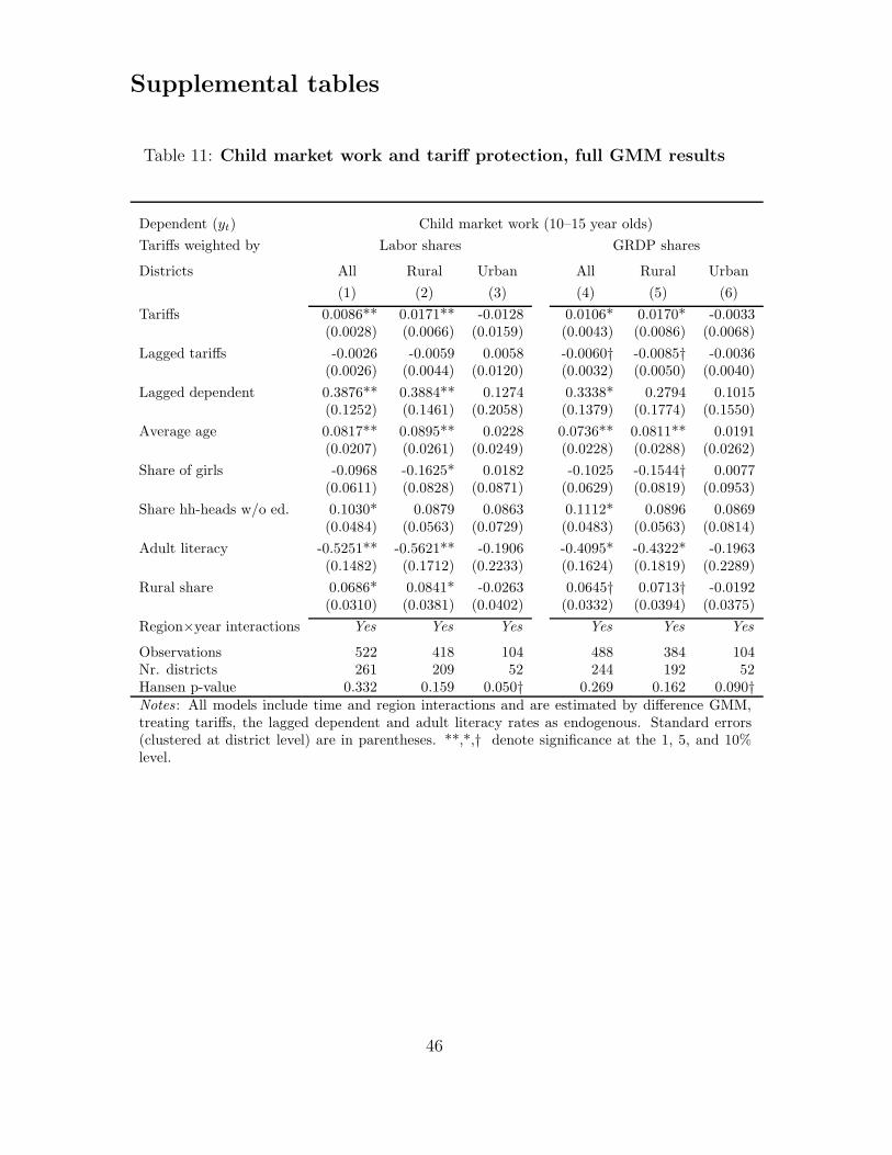
Supplemental tables
Table 11: Child market work and tariff protection, full GMM results
Dependent (𝑦𝑡) Child market work (10–15 year olds)
Tariffs weighted by Labor shares GRDP shares
Districts All Rural Urban All Rural Urban
(1) (2) (3) (4) (5) (6)
Tariffs 0.0086** 0.0171** -0.0128 0.0106* 0.0170* -0.0033(0.0028) (0.0066) (0.0159) (0.0043) (0.0086) (0.0068)
Lagged tariffs -0.0026 -0.0059 0.0058 -0.0060† -0.0085† -0.0036(0.0026) (0.0044) (0.0120) (0.0032) (0.0050) (0.0040)
Lagged dependent 0.3876** 0.3884** 0.1274 0.3338* 0.2794 0.1015(0.1252) (0.1461) (0.2058) (0.1379) (0.1774) (0.1550)
Average age 0.0817** 0.0895** 0.0228 0.0736** 0.0811** 0.0191(0.0207) (0.0261) (0.0249) (0.0228) (0.0288) (0.0262)
Share of girls -0.0968 -0.1625* 0.0182 -0.1025 -0.1544† 0.0077(0.0611) (0.0828) (0.0871) (0.0629) (0.0819) (0.0953)
Share hh-heads w/o ed. 0.1030* 0.0879 0.0863 0.1112* 0.0896 0.0869(0.0484) (0.0563) (0.0729) (0.0483) (0.0563) (0.0814)
Adult literacy -0.5251** -0.5621** -0.1906 -0.4095* -0.4322* -0.1963(0.1482) (0.1712) (0.2233) (0.1624) (0.1819) (0.2289)
Rural share 0.0686* 0.0841* -0.0263 0.0645† 0.0713† -0.0192(0.0310) (0.0381) (0.0402) (0.0332) (0.0394) (0.0375)
Region×year interactions Yes Yes Yes Yes Yes Yes
Observations 522 418 104 488 384 104Nr. districts 261 209 52 244 192 52Hansen p-value 0.332 0.159 0.050† 0.269 0.162 0.090†Notes : All models include time and region interactions and are estimated by difference GMM,treating tariffs, the lagged dependent and adult literacy rates as endogenous. Standard errors(clustered at district level) are in parentheses. **,*,† denote significance at the 1, 5, and 10%level.
46
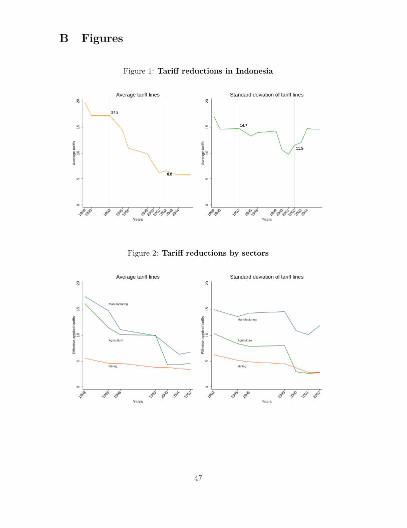
B Figures
Figure 1: Tariff reductions in Indonesia
17.2
6.6
17.2
6.6
17.2
6.6
05
1015
20A
vera
ge ta
riffs
1989
1990
1993
1995
1996
1999
2000
2001
2002
2003
2004
Years
Average tariff lines
14.7
11.5
14.7
11.5
14.7
11.5
05
1015
20A
vera
ge ta
riffs
1989
1990
1993
1995
1996
1999
2000
2001
2002
2003
2004
Years
Standard deviation of tariff lines
Figure 2: Tariff reductions by sectors
Agriculture
Mining
Manufacturing
05
1015
20E
ffect
ive
appl
ied
tarif
fs
1993
1995
1996
1999
2000
2001
2002
Years
Average tariff lines
Agriculture
Mining
Manufacturing
05
1015
20E
ffect
ive
appl
ied
tarif
fs
1993
1995
1996
1999
2000
2001
2002
Years
Standard deviation of tariff lines
47
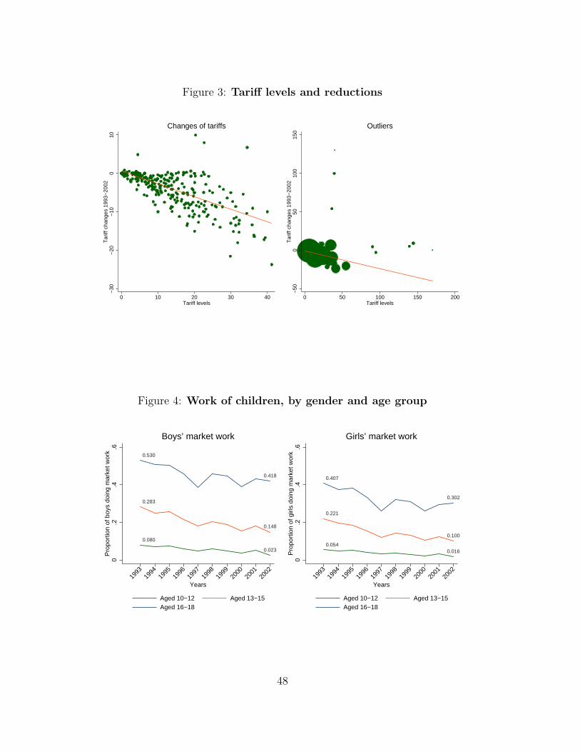
Figure 3: Tariff levels and reductions
−30
−20
−10
010
Tar
iff c
hang
es 1
993−
2002
0 10 20 30 40Tariff levels
Changes of tariffs
−50
050
100
150
Tar
iff c
hang
es 1
993−
2002
0 50 100 150 200Tariff levels
Outliers
Figure 4: Work of children, by gender and age group
0.080
0.023
0.283
0.148
0.530
0.418
0.2
.4.6
Pro
port
ion
of b
oys
doin
g m
arke
t wor
k
1993
1994
1995
1996
1997
1998
1999
2000
2001
2002
Years
Aged 10−12 Aged 13−15Aged 16−18
Boys’ market work
0.0540.016
0.221
0.100
0.407
0.302
0.2
.4.6
Pro
port
ion
of g
irls
doin
g m
arke
t wor
k
1993
1994
1995
1996
1997
1998
1999
2000
2001
2002
Years
Aged 10−12 Aged 13−15Aged 16−18
Girls’ market work
48
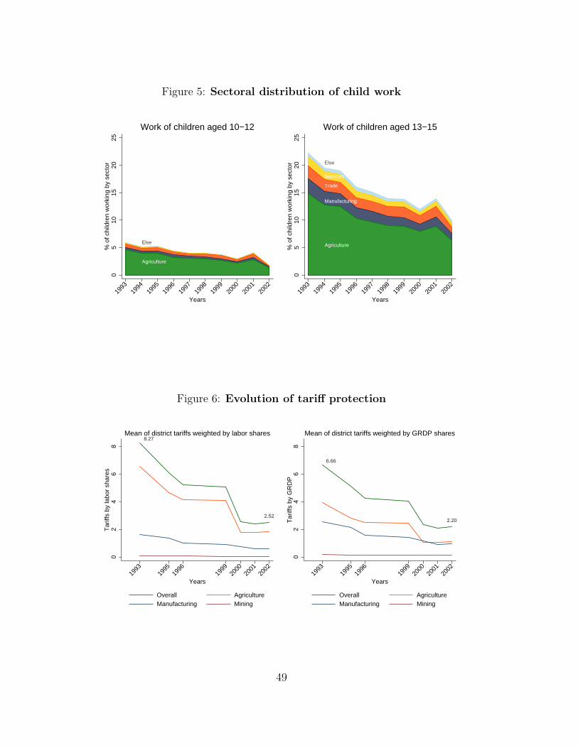
Figure 5: Sectoral distribution of child work
Agriculture
Else
05
1015
2025
% o
f chi
ldre
n w
orki
ng b
y se
ctor
1993
1994
1995
1996
1997
1998
1999
2000
2001
2002
Years
Work of children aged 10−12
Agriculture
Manufacturing
Trade
Services
Else
05
1015
2025
% o
f chi
ldre
n w
orki
ng b
y se
ctor
1993
1994
1995
1996
1997
1998
1999
2000
2001
2002
Years
Work of children aged 13−15
Figure 6: Evolution of tariff protection
8.27
2.52
02
46
8T
ariff
s by
labo
r sh
ares
1993
1995
1996
1999
2000
2001
2002
Years
Overall AgricultureManufacturing Mining
Mean of district tariffs weighted by labor shares
6.66
2.20
02
46
8T
ariff
s by
GR
DP
1993
1995
1996
1999
2000
2001
2002
Years
Overall AgricultureManufacturing Mining
Mean of district tariffs weighted by GRDP shares
49
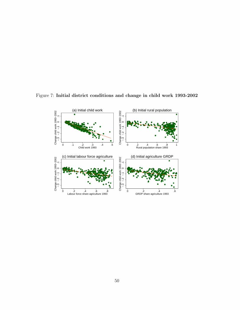
Figure 7: Initial district conditions and change in child work 1993-2002
−.3
−.2
−.1
0.1
Cha
nge
child
wor
k 19
93−
2002
0 .1 .2 .3 .4 .5Child work 1993
(a) Initial child work
−.3
−.2
−.1
0.1
Cha
nge
child
wor
k 19
93−
2002
0 .2 .4 .6 .8 1Rural population share 1993
(b) Initial rural population
−.3
−.2
−.1
0.1
Cha
nge
child
wor
k 19
93−
2002
0 .2 .4 .6 .8Labour force share agriculture 1993
(c) Initial labour force agriculture
−.3
−.2
−.1
0.1
Cha
nge
child
wor
k 19
93−
2002
0 .2 .4 .6GRDP share agriculture 1993
(d) Initial agriculture GRDP
50


