
University of Kentucky University of Kentucky
UKnowledge UKnowledge
Theses and Dissertations--Plant and Soil Sciences Plant and Soil Sciences
2018
CHARACTERIZING NITROGEN LOSS AND GREENHOUSE GAS CHARACTERIZING NITROGEN LOSS AND GREENHOUSE GAS
FLUX ACROSS AN INTENSIFICATION GRADIENT IN DIVERSIFIED FLUX ACROSS AN INTENSIFICATION GRADIENT IN DIVERSIFIED
VEGETABLE SYSTEMS VEGETABLE SYSTEMS
Debendra Shrestha University of Kentucky, [email protected] Author ORCID Identifier:
https://orcid.org/0000-0002-4594-078X Digital Object Identifier: https://doi.org/10.13023/etd.2018.460
Right click to open a feedback form in a new tab to let us know how this document benefits you. Right click to open a feedback form in a new tab to let us know how this document benefits you.
Recommended Citation Recommended Citation Shrestha, Debendra, "CHARACTERIZING NITROGEN LOSS AND GREENHOUSE GAS FLUX ACROSS AN INTENSIFICATION GRADIENT IN DIVERSIFIED VEGETABLE SYSTEMS" (2018). Theses and Dissertations--Plant and Soil Sciences. 111. https://uknowledge.uky.edu/pss_etds/111
This Doctoral Dissertation is brought to you for free and open access by the Plant and Soil Sciences at UKnowledge. It has been accepted for inclusion in Theses and Dissertations--Plant and Soil Sciences by an authorized administrator of UKnowledge. For more information, please contact [email protected].

STUDENT AGREEMENT: STUDENT AGREEMENT:
I represent that my thesis or dissertation and abstract are my original work. Proper attribution
has been given to all outside sources. I understand that I am solely responsible for obtaining
any needed copyright permissions. I have obtained needed written permission statement(s)
from the owner(s) of each third-party copyrighted matter to be included in my work, allowing
electronic distribution (if such use is not permitted by the fair use doctrine) which will be
submitted to UKnowledge as Additional File.
I hereby grant to The University of Kentucky and its agents the irrevocable, non-exclusive, and
royalty-free license to archive and make accessible my work in whole or in part in all forms of
media, now or hereafter known. I agree that the document mentioned above may be made
available immediately for worldwide access unless an embargo applies.
I retain all other ownership rights to the copyright of my work. I also retain the right to use in
future works (such as articles or books) all or part of my work. I understand that I am free to
register the copyright to my work.
REVIEW, APPROVAL AND ACCEPTANCE REVIEW, APPROVAL AND ACCEPTANCE
The document mentioned above has been reviewed and accepted by the student’s advisor, on
behalf of the advisory committee, and by the Director of Graduate Studies (DGS), on behalf of
the program; we verify that this is the final, approved version of the student’s thesis including all
changes required by the advisory committee. The undersigned agree to abide by the statements
above.
Debendra Shrestha, Student
Dr. Krista Jacobsen, Major Professor
Dr. Mark Coyne, Director of Graduate Studies

CHARACTERIZING NITROGEN LOSS AND GREENHOUSE GAS FLUX ACROSS AN INTENSIFICATION GRADIENT IN DIVERSIFIED VEGETABLE SYSTEMS
________________________________________
DISSERTATION ________________________________________
A dissertation submitted in partial fulfillment of the requirements for the degree of Doctor of Philosophy in the
College of Agriculture, Food and Environment at the University of Kentucky
By
Debendra Shrestha
Lexington, Kentucky
Co- Directors: Dr. Krista Jacobsen, Associate Professor, Department of Horticulture
and Dr. Ole Wendroth, Professor, Department of Plant and Soil Sciences
Lexington, Kentucky
2018
Copyright © Debendra Shrestha 2018
https://orcid.org/0000-0002-4594-078X

ABSTRACT OF DISSERTATION
CHARACTERIZING NITROGEN LOSS AND GREENHOUSE GAS FLUX
ACROSS AN INTENSIFICATION GRADIENT IN DIVERSIFIED VEGETABLE
SYSTEMS
The area of vegetable production is growing rapidly world-wide, as are efforts to
increase production on existing lands in these labor- and input-intensive systems. Yet
information on nutrient losses, greenhouse gas emissions, and input efficiency is lacking.
Sustainable intensification of these systems requires knowing how to optimize nutrient
and water inputs to improve yields while minimizing negative environmental
consequences. This work characterizes soil nitrogen (N) dynamics, nitrate (NO3¯)
leaching, greenhouse gas emissions, and crop yield in five diversified vegetable systems
spanning a gradient of intensification that is characterized by inputs, tillage and rotational
fallow periods. The study systems included a low input organic system (LI), a
mechanized, medium scale organic system (CSA), an organic movable high tunnel
system (MOV), a conventional system (CONV) and an organic stationary high tunnel
system (HT). In a three-year vegetable crop rotation with three systems (LI, HT and
CONV), key N loss pathways varied by system; marked N2O and CO2 losses were
observed in the LI system and NO3– leaching was greatest in the CONV system. Yield-
scaled global warming potential (GWP) was greater in the LI system compared to HT and
CONV, driven by greater greenhouse gas flux and lower yields in the LI system. The
field data from CONV system were used to calibrate the Root Zone Water Quality Model
version 2 (RZWQM2) and HT and LI vegetable systems were used to validate the model.
RZWQM2 simulated soil NO3¯-N content reasonably well in crops grown on bare
ground and open field (e.g. beet, collard, bean). Despite use of simultaneous heat and
water (SHAW) option in RZWQM2 to incorporate the use of plastic mulch, we were not
able to successfully simulate NO3¯-N data. The model simulated cumulative N2O
emissions from the CONV vegetable system reasonably well, while the model
overestimated N2O emissions in HT and LI systems.

KEYWORDS: Sustainable Intensification, Vegetables, Nitrogen Dynamics, N2O and CO2 Emissions, Organic Farming, RZWQM2
Debendra Shrestha
11/20/2018 Date

CHARACTERIZING NITROGEN LOSS AND GREENHOUSE GAS FLUX
ACROSS AN INTENSIFICATION GRADIENT IN DIVERSIFIED VEGETABLE SYSTEMS
By Debendra Shrestha
Dr. Krista Jacobsen Co-Director of Dissertation
Dr. Ole Wendroth
Co-Director of Dissertation
Dr. Mark Coyne Director of Graduate Studies
11/20/2018
Date

DEDICATION
To my Family

iii
ACKNOWLEDGMENTS
I feel a great pleasure to express my profound sense of gratitude, veneration and
indebtedness to Dr. Krista Jacobsen, Associate Professor, Department of Horticulture and
Dr. Ole Wendroth, Professor, Department of Plant and Soil Sciences, University of
Kentucky; Co-directors of my advisory committee for their continuous support,
encouragement, supervision, and constant guidance throughout the experiment period and
during the preparation of this dissertation.
It gives me immense pleasure to express my reverential regards to honorable
members of my advisory committee Dr. Mark Coyne, Professor and Dr. Wei Ren,
Assistant Professor Department of Plant and Soil Sciences; Dr. Mark Williams, Dr. Brent
Rowell, and Dr. Richard Durham, Professors, Department of Horticulture, University of
Kentucky for their support and suggestions.
I would like to express thanks to USDA Agriculture and Food Research Initiative
(AFRI) for providing funding for research work.
I am also thankful to Department of Horticulture family, UK Horticulture
Research Farm, UK Community Supported Agriculture (UK CSA), McCully Lab, and
Elmwood Stock Farm. I am heartily thankful to Dr. Alexandra Williams, Brett Wolff.
Jennifer Taylor, Jason Riley Walton, Ann Freytag, Dr. Haichao Guo, Aaron Stancombe,
Savannah McGuire, Ellen Green, Rebecca Shelton, David Smith, and Maria Cruz for
laboratory and field assistance on this project.
I would express my heartiest gratitude and respect to my beloved parents; my
wife Sapana Shrestha for her continuous support, love and helping in my research; lovely
daughter Divaasna whose smiles relieved my work stress away every day; Bishnu Didi
and Hari Bhinaju, Suman dai and Bhauju, Mahendra and Ela, Ashim and Ashma, Mother
in Law Sarita Shrestha, Bishnu Nini for always being there for me and Sapana.

iv
TABLE OF CONTENTS
ACKNOWLEDGMENTS ................................................................................................. iii
LIST OF TABLES ............................................................................................................ vii
LIST OF FIGURES ......................................................................................................... viii
CHAPTER 1. INTRODUCTION ....................................................................................... 1
1.1 Sustainable intensification in vegetable systems .................................................... 1 1.1.1 Fertilizers ........................................................................................................ 3 1.1.2 Irrigation ......................................................................................................... 5 1.1.3 Crop rotation and managed fallow periods ..................................................... 6 1.1.4 Effect of intensification on yields ................................................................... 8
1.2 Nitrogen dynamics in vegetable cropping systems ............................................... 11 1.2.1 N cycling and retention ................................................................................. 11 1.2.2 N leaching in vegetable cropping system ..................................................... 12 1.2.3 Trace gas emissions ...................................................................................... 13
1.3 Simulation modelling in vegetable production systems ....................................... 15
CHAPTER 2. NITROGEN LOSS AND GREENHOUSE GAS FLUX ACROSS AN INTENSIFICATION GRADIENT IN DIVERSIFIED VEGETABLE ROTATIONS .... 19
2.1 Introduction ........................................................................................................... 19
2.2 Materials and Methods .......................................................................................... 22 2.2.1 Research sites ................................................................................................ 22 2.2.2 Cropping systems .......................................................................................... 22 2.2.3 Soil sampling ................................................................................................ 24 2.2.4 Plant sampling ............................................................................................... 27 2.2.5 Statistical analysis ......................................................................................... 27
2.3 Results ................................................................................................................... 28 2.3.1 Time series data ............................................................................................ 28
2.3.1.1 Low input system .................................................................................. 28 2.3.1.2 Conventional system ............................................................................. 29 2.3.1.3 High tunnel system ............................................................................... 30
2.3.2 Cumulative CO2 and N2O fluxes .................................................................. 31 2.3.3 Yield and yield scaled GWP ......................................................................... 32
2.4 Discussion ............................................................................................................. 32 2.4.1 Soil mineral N ............................................................................................... 32

v
2.4.2 Soil water content measurements.................................................................. 34 2.4.3 Trace gases .................................................................................................... 35 2.4.4 Harvested crop yields .................................................................................... 36 2.4.5 Sustainable intensification of horticultural systems ..................................... 37
2.5 Conclusion ............................................................................................................ 38
2.6 Tables and figures ................................................................................................. 39
CHAPTER 3. USING RZWQM2 TO SIMULATE NITROGEN DYNAMICS AND NITROUS OXIDE EMISSIONS IN VEGETABLE PRODUDUCTION SYSTEMS .... 47
3.1 Introduction ........................................................................................................... 47
3.2 Materials and methods .......................................................................................... 50 3.2.1 Research sites ................................................................................................ 50 3.2.2 Cropping systems description ....................................................................... 50 3.2.3 Measured data ............................................................................................... 51 3.2.4 Model description ......................................................................................... 52 3.2.5 Model input, calibration and validation ........................................................ 55
3.3 Results and discussion .......................................................................................... 58 3.3.1 Soil temperature ............................................................................................ 58 3.3.2 Soil water content ......................................................................................... 58 3.3.3 Soil nitrate content ........................................................................................ 59 3.3.4 Nitrous oxide emissions ................................................................................ 62 3.3.5 Crop yield and biomass ................................................................................. 66 3.3.6 Model simulated outputs through the soil profile ......................................... 67
3.4 Conclusion ............................................................................................................ 67
3.5 Tables and figures ................................................................................................. 69
CHAPTER 4. CHARACTERIZING THE SUSTAINABILITY OF INTENSIFICATION IN VEGETABLE SYSTEMS ........................................................................................... 82
4.1 Introduction ........................................................................................................... 82
4.2 Materials and methods .......................................................................................... 83 4.2.1 Cropping systems .......................................................................................... 84
4.2.1.1 Low input system (LI) ......................................................................... 84 4.2.1.2 Community supported agriculture system (CSA) ................................. 85 4.2.1.3 Movable high tunnel system (MOV) .................................................... 86 4.2.1.4 Conventional system (CONV) .............................................................. 86 4.2.1.5 High tunnel system (HT) ...................................................................... 87
4.2.2 Model crops and management ...................................................................... 88 4.2.3 Soil sampling ................................................................................................ 89

vi
4.2.4 Yield and plant biomass sampling ................................................................ 89
4.3 Results and discussion .......................................................................................... 90 4.3.1 Fresh vegetable yield .................................................................................... 90 4.3.2 N leaching ..................................................................................................... 91 4.3.3 Soil mineral N content .................................................................................. 92 4.3.4 N uptake relative to fertilization ................................................................... 93
4.4 Conclusion ............................................................................................................ 94
4.5 Tables and figures ................................................................................................. 96
CHAPTER 5. CONCLUSIONS ..................................................................................... 103
REFERENCES ............................................................................................................... 105
VITA ............................................................................................................................... 129

vii
LIST OF TABLES Table 2.1 Initial soil conditions at study depths of three study agroecosystems. ............. 39
Table 2.2 Management characterization of three study agroecosystems, as characterized by cropping system duration, and tillage, nutrient and irrigation input intensities........... 40
Table 2.3 Crop timing and fertilizer rates in three study agroecosystems. Timing of the crop rotation is detailed by planting date (PD) to final termination date (TD) by primary tillage or crop removal. ..................................................................................................... 41
Table 2.4 Spearman rank correlation values for N2O flux and soil mineral nitrogen (NO3¯-N and NH4
+-N) and soil temperature, and carbon dioxide flux and soil temperature in three study vegetable production systems. ............................................... 42
Table 3.1 Measured soil bulk density (BD) and texture and calibrated saturated hydraulic conductivity (Ksat), saturation (θs), 1/3 bar (θ1/3), 15 bar (θ15) and residual (θr) soil water content ............................................................................................................................... 69
Table 3.2 Measured and simulated daily average temperature, R2 and RMSE values of soil temperature (ST) in Conventional (CONV), High Tunnel Organic (HT), and Low Input (LI) system during 2014-2016. ................................................................................ 70
Table 3.3 Measured and simulated average, R2 and RMSE values of volumetric soil water content in Conventional (CONV), High Tunnel Organic (HT), and Low Input (LI) system during 2014-2016. ............................................................................................................. 71
Table 3.4 Measured and simulated average, R2 and RMSE values of soil NO3¯-N content in Conventional (CONV), High Tunnel Organic (HT), and Low Input (LI) system during 2014-2016. ........................................................................................................................ 72
Table 3.5 Measured and simulated cumulative N2O-N flux during each crop period, R2
and RMSE values in Conventional (CONV), High Tunnel Organic (HT), and Low Input (LI) system during 2014-2016. ......................................................................................... 73
Table 3.6 Measured and simulated crop yield during the cropping season 2014-2016. ... 74
Table 3.7 Simulated soil N processes and loss pathways from 100 cm soil profile in three vegetable systems.............................................................................................................. 75
Table 4.1 Fertility and irrigation management for model crops in the five study systems............................................................................................................................................ 96
Table 4.2 Mean marketable (USDA grades 1&2) fresh yield of pepper, beet and collard from 2014, 2015 and 2016 in the five study systems. ...................................................... 98
Table 4.3 The averages soil NO3¯-N during pepper, beet and collard growing season from 2014, 2015, and 2016 in low input, community supported agriculture, movable high tunnel, conventional and high tunnel system .................................................................... 99
Table 4.4 The Average crop N uptake and N fertilizer applied in five systems. ............ 100
viii
LIST OF FIGURES
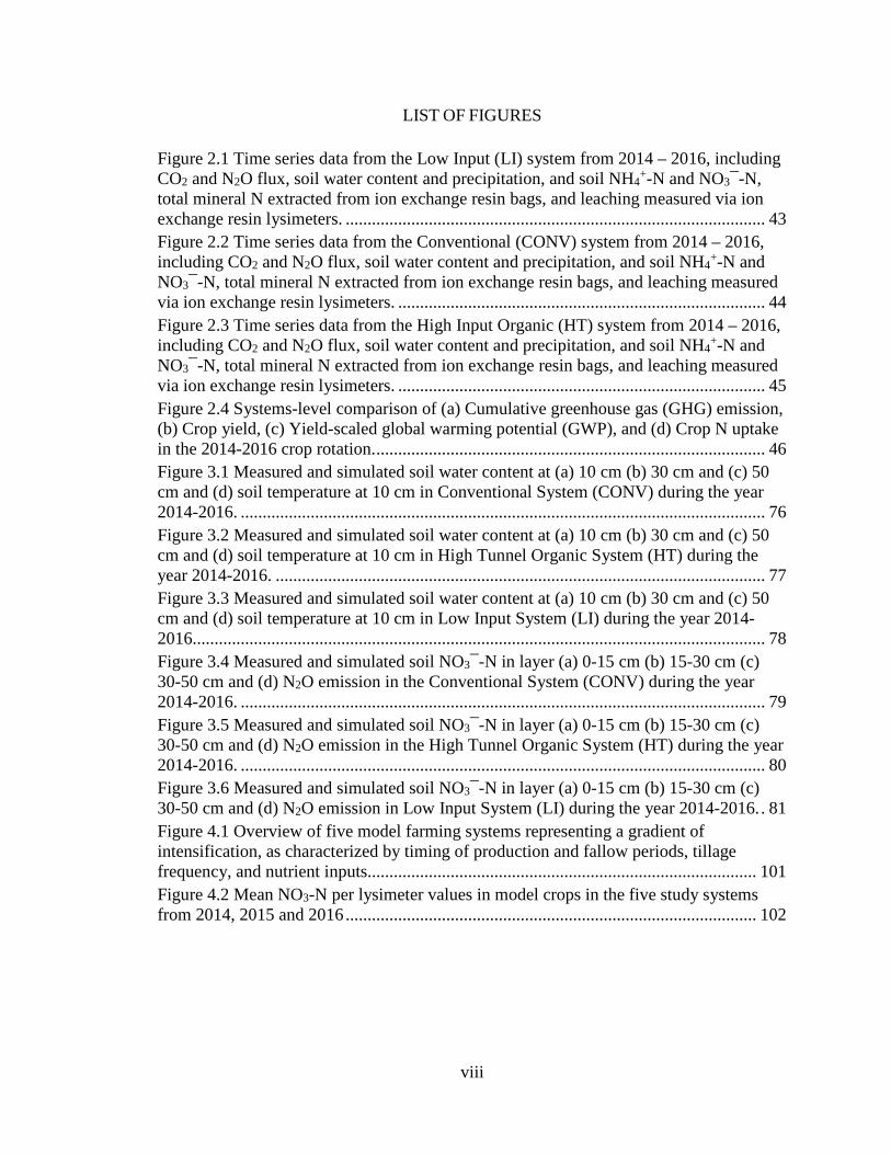
Figure 2.1 Time series data from the Low Input (LI) system from 2014 – 2016, including CO2 and N2O flux, soil water content and precipitation, and soil NH4
+-N and NO3¯-N, total mineral N extracted from ion exchange resin bags, and leaching measured via ion exchange resin lysimeters. ................................................................................................ 43 Figure 2.2 Time series data from the Conventional (CONV) system from 2014 – 2016, including CO2 and N2O flux, soil water content and precipitation, and soil NH4
+-N and NO3¯-N, total mineral N extracted from ion exchange resin bags, and leaching measured via ion exchange resin lysimeters. .................................................................................... 44 Figure 2.3 Time series data from the High Input Organic (HT) system from 2014 – 2016, including CO2 and N2O flux, soil water content and precipitation, and soil NH4
+-N and NO3¯-N, total mineral N extracted from ion exchange resin bags, and leaching measured via ion exchange resin lysimeters. .................................................................................... 45 Figure 2.4 Systems-level comparison of (a) Cumulative greenhouse gas (GHG) emission, (b) Crop yield, (c) Yield-scaled global warming potential (GWP), and (d) Crop N uptake in the 2014-2016 crop rotation. ......................................................................................... 46 Figure 3.1 Measured and simulated soil water content at (a) 10 cm (b) 30 cm and (c) 50 cm and (d) soil temperature at 10 cm in Conventional System (CONV) during the year 2014-2016. ........................................................................................................................ 76 Figure 3.2 Measured and simulated soil water content at (a) 10 cm (b) 30 cm and (c) 50 cm and (d) soil temperature at 10 cm in High Tunnel Organic System (HT) during the year 2014-2016. ................................................................................................................ 77 Figure 3.3 Measured and simulated soil water content at (a) 10 cm (b) 30 cm and (c) 50 cm and (d) soil temperature at 10 cm in Low Input System (LI) during the year 2014-2016................................................................................................................................... 78 Figure 3.4 Measured and simulated soil NO3¯-N in layer (a) 0-15 cm (b) 15-30 cm (c) 30-50 cm and (d) N2O emission in the Conventional System (CONV) during the year 2014-2016. ........................................................................................................................ 79 Figure 3.5 Measured and simulated soil NO3¯-N in layer (a) 0-15 cm (b) 15-30 cm (c) 30-50 cm and (d) N2O emission in the High Tunnel Organic System (HT) during the year 2014-2016. ........................................................................................................................ 80 Figure 3.6 Measured and simulated soil NO3¯-N in layer (a) 0-15 cm (b) 15-30 cm (c) 30-50 cm and (d) N2O emission in Low Input System (LI) during the year 2014-2016. . 81 Figure 4.1 Overview of five model farming systems representing a gradient of intensification, as characterized by timing of production and fallow periods, tillage frequency, and nutrient inputs......................................................................................... 101 Figure 4.2 Mean NO3-N per lysimeter values in model crops in the five study systems from 2014, 2015 and 2016 .............................................................................................. 102

1
CHAPTER 1. INTRODUCTION
1.1 Sustainable intensification in vegetable systems
Meeting society’s growing need for food while minimizing harm to the natural
resource base upon which food production depends has been characterized as the
collective “grand challenge” for agriculture (Foley et al., 2011). There is broad
understanding that this challenge must be met largely on existing agricultural lands, and
through managing natural resources more efficiently than they are currently (FAO, 2011;
Tilman et al., 2011). Sustainable intensification invokes environmental goals such as
optimizing the use of external inputs (Matson et al., 1997; Pretty 1997, 2008), increasing
rates of internal nutrient recycling, decreasing nutrient loss (Gliessman, 2007), and
closing yield gaps (Mueller et al., 2012; Pradhan et al., 2015; Wezel et al., 2015). To
date, intensification efforts have focused largely on staple grain systems, but efforts to
sustainably intensify fruit and vegetable production systems are particularly timely due to
a suite of economic and environmental factors.
Similar to all sectors of crop and livestock production, global vegetable
production has increased substantially in the past 50 years, with rising population growth
and intensification of agricultural production systems (FAOSTAT, 2018). The five-fold
increase observed in global vegetable yields since 1961 is a function of both increasing
production area and increasing productivity on existing lands in production. This increase
is largely due to conversion of lands from staple grain production to high-value specialty
crops, particularly in small-holder farming areas experiencing declining grain prices
(Weinberger and Lumpkin, 2007). The dual trends of diversification into vegetable
production and intensifying production systems has been particularly strong in Asia,
2
where highly intensive, protected agricultural production systems (e.g. plastic-covered
greenhouse systems) have grown exponentially since 1980 (Norse et al., 2014). In the
U.S., the number of vegetable farms has consistently increased, and although vegetable
farms are typically smaller in production area, the total average value of produce sales
per unit area is greater than average grain crop farms.
As such, production of vegetables and other high value specialty crops have
created pathways for farmers to enter or remain in agriculture worldwide, with
commensurate increase in global vegetable yields and area under specialty crop
production. Weinberger and Lumpkin (2007) dubbed this trend “a silent horticultural
revolution.” Certainly, there are significant benefits to increased production of nutritious,
high value crops for farmers and the global food system. However, vegetable production
systems span a gradient of production intensity, from very low external input, to arguably
among the highest in water, nutrient, and agrochemical application. Such diversity in
production practices does not lend to uniform management practices or consistent
recommendations to sustainably intensify these expanding production systems.
Traditionally, vegetable production often involves repeated tillage, bare soil, and
significant use of fertilizers, pesticides, and water. In the long-term, these practices can
reduce productivity and profitability of a production system. As such, there is a growing
need for production practices and management techniques that can increase or at least
stabilize productivity and profitability while increasing the efficiency of inputs while
minimizing environmental impacts (Wells et al., 2000).
Sustainable intensification has been proposed to increase crop yield with minimal
loss of biodiversity, nutrients, soil, and greenhouse gas emissions. Further, the

3
sustainability of the production systems should also be associated with temporal and
spatial stability of yield as it relates to changes key soil properties (Schrama et al., 2018).
Agricultural intensification and the resulting increases in yields have mainly been
attributed to intensive irrigation practices, agrochemical inputs and intensive tillage. Due
to problems of environmental degradation and perceived public health risk, there is
growing interest in alternative farming systems including organic (no synthetic fertilizer
and pesticide use) and low-input farming systems, which are being explored as ways to
improve overall soil health, agricultural sustainability, and environmental quality (Poudel
et al., 2002). However, more study of alternative production systems is needed to
understand how input use and production practices in these systems affect environmental
factors (Clark and Tilman, 2017). In the sections below, the literature regarding particular
aspects of agricultural intensification are reviewed, including nutrient and irrigation use,
use of fallow periods, and their effects on yield.
1.1.1 Fertilizers
Fertilizer use in vegetable crops is routine. For example, 98 percent of tomato
production area was fertilized in the US in 2010 at the rate of 160 kg N ha-1 (USDA
NASS, 2011). This is relatively high rate in comparison to other agricultural systems (e.g.
small grains, forages, etc.) in the U.S. However, it pales in comparison to excessive rates
applied in horticultural systems in input-intensive regions in the world. For example, N
fertilizer use has been documented to be as high as 1000 kg ha-1 in covered vegetable
areas of China (Zhu et al., 2005; Ju et al., 2007). Although increased N fertilization rates
within a certain range have been shown to directly correlate to increases in crop yields in
certain crop families (e.g. cole crops, Congreves et al., 2015), the effect of increased
4
fertilizer rates may be negated by the greater influence of climate (temperature and
precipitation) on crop yield. A recent study by Cui et al. (2018) demonstrated a 7.8-9.5
Mg ha-1 increase in grain yield with enhanced management practice, while at the same
time reducing N fertilizer application (kg N per unit area) by 8.5-15.6 %. Further, a 23-35
% decrease in reactive N losses (N2O emission, NH3 volatilization, NO3¯ leaching) and
19-29 % reduction in greenhouse gas emission were achieved (Cui et al., 2018). The
efficiency of fertilizer uptake by crop plants, particularly N fertilizers, and the
environmental fate of fertilizer losses vary by the nature of the fertilizer. Mineral N
fertilizer is commonly applied in mineral (inorganic) form as urea and solutions of urea
and ammonium nitrate, with urea being most readily volatilized as ammonia (Battye et
al., 1994). The use of “complete” fertilizer (containing N-P-K) is also common in
vegetable production (Blatt and McRae, 1988), with the N component of these fertilizers
generally consisting of urea and ammoniacal N.
In low-input and organic systems there is greater reliance on organic N sources,
such as manures, composts, and byproducts of animal and plant processing industries
(Gaskell and Smith, 2007). These are used in combination with crop rotations that often
include annual and perennial cover crops or forages. Internal N cycling in these systems
more closely mimic natural systems (Dawson et al., 2008). Compost, a source of plant
nutrients, is also commonly used in organic and conventional vegetable production
systems. In organic production systems, compost use is typically augmented with organic
fertilizers during peak production and late season at periods of peak crop N demand
(Gaskell and Smith, 2007). However, the uncertainty of nutrient content and availability
in these biological amendments can lead to over or under-fertilization, build up and

5
leaching of nutrients, or lack of synchrony between nutrient supply and plant uptake
(Drinkwater and Snapp, 2007). It is necessary to understand how organic inputs and their
management influence the temporal dynamics of soil inorganic N availability in the
context of the farming system to balance the essential soil functions of providing crop
fertility while reducing N losses to the environment (Norris and Congreves, 2018).
1.1.2 Irrigation
Vegetables are often irrigated. Surface and sub-surface drip irrigation has been
increasingly used to irrigate vegetable crops around the world. Relative to other methods
of irrigation such as flood, furrow or sprinkler irrigation systems, drip irrigation has
greater water use efficiency than other water application methods (Darwish et al., 2003).
Drip irrigation has been consistently shown to increase crop yield and water use
efficiency in vegetable production systems (e.g. Singadhupe et al., 2003; Yaghi et al.,
2013). Drip irrigation provides water directly to the plant root zone, and when coupled
with practices that supply water in small quantity but frequent application, generally
produces higher ratios of yield per unit area and yield per unit volume of water than
typical surface or sprinkler systems (Darwish et al., 2003). In rain-protected agriculture
systems, including high tunnels, all water is supplied via irrigation. Drip irrigation is the
recommended irrigation method in these systems. Although all crop water is supplied via
irrigation, the use of water is often reduced compared to irrigated open field production
due to evapotranspiration loss (Fernandez et al., 2007). Some of the greatest growth in
vegetable production systems has been in the use of such protected culture systems which
include the use of greenhouses and polyethylene tunnels (e.g. high tunnels, hoop houses)
in which vegetables are grown in-ground in a semi-controlled environment. Growth in

6
horticultural crops produced in protected culture rose by 44% from 2009 to 2014 (USDA
NASS, 2014). This pales in comparison to the adoption of protected agriculture in China,
which accounts for 90% of global greenhouse structures (Chang et al., 2013) through
rapid intensification of the agriculture sector since the 1980’s (Norse and Ju, 2015). Yield
in the protected agriculture can be twice as high as that over open culture (Chang et al.,
2013). High tunnels are also commonly used to produce high value crops. With proper
planning and management techniques, high tunnels can optimize yields, increase fruit
quality, and provide season extension opportunities for high-value vegetable crops
(O’Connell et al., 2012). Generally, high tunnels provide the opportunity for earlier crop
planting and earlier harvest compared to open field conditions. O’Connell et al. (2012)
reported similar yield in the first year and 33 % more tomato yield in the second year in
high tunnels compared to open field conditions.
1.1.3 Crop rotation and managed fallow periods
Crop rotation is a key strategy to control environmental stresses and improve crop
performance in conventional and organic vegetable systems. However, the need for
biological inputs to replace synthetic inputs, and an emphasis on soil organic matter
management in organic production drive organic growers to adopt major changes
compared to their conventional counterparts. Higher cover crop diversity, frequent cover
crop rotation, use of legume crops, and intercropping are more common in low input and
organic farming. The increased complexity and diversity of crop rotations are likely to
provide strong environmental benefits and enhanced ecosystem services (Barbieri et al.,
2017), although more study of how the elements of rotation, tillage, cover crop use, and
fertilizers/amendments interact is needed.

7
Cover crops, such as annual grasses or legumes, are often included between
vegetable crops to prevent erosion, provide organic matter and nutrients for subsequent
crops and minimize leaching (Thorup-Kristensen et al., 2003; Robacer et al., 2016).
Although cover crops are not able to provide enough total N for a high N-demanding
vegetable crop, or mineralize in synchrony with plant N demand (Drinkwater and Snapp,
2007) they may still increase the net economic returns (Muramoto et al., 2011) by
trapping N otherwise lost. In temperate regions, cool season cover crops are most
common, and are planted in the late summer or early fall, after harvest of warm season
vegetables. They are terminated in the subsequent spring prior to planting. They may also
be used in other temporal windows in the rotation vegetable systems. For example short-
season summer cover crops provide weed suppression and nutrients for fall-planted
vegetable crops (Creamer and Baldwin, 2000).
The interaction between cover crops (managed fallow) and the subsequent crop
fertility regime affects the nature and magnitude of nutrient input losses in
agroecosystems. Shelton et al. (2018) quantified N loss via leaching, NH3 volatilization,
N2O emissions, and N retention in plant and soil pools of corn agroecosystems in
Kentucky. Cover crop species and fertilization schemes affect N loss and availability in
corn systems and dominant N loss pathways varied by season. NO3¯-N leaching was the
primary loss pathway during the cover crop growing season, especially in treatments
using leguminous monocultures (hairy vetch only), while N loss via N2O-N and NH3-N
emissions was dominant during the corn growing season. Nitrogen contribution of
legume-grass cover crop mixture into fertilizer application rates may reduce N loss
without sacrificing yield (Han et al., 2017).

8
Pasture-crop rotations, which utilize a multiple year period of grazed pasture
fallow followed by crop production, are popular in Argentina, Brazil, and Uruguay
(Garcia-Prechac et al., 2004) and have significant effects on soil properties. Soil
aggregate stability increases quickly by including pasture in the rotation with crops, due
to the combination of a) the absence of tillage operation during the pasture cycle; (b) the
dense and fibrous grass root systems that promote aggregation (Haynes et al., 1991). The
combined use of cropping and pasture in rotation results in reduced soil erosion
compared to continuous cropping (Garcia-Prechac et al., 2004). Agricultural soils benefit
from the re-introducing perennial grasses and legumes into the crop field by gaining
organic matter and strengthening their capacity for long-term productivity and
environmental resiliency (Franzluebers et al., 2014). Crop-pasture rotation systems, as
reported by Franzluebbers et al. (2014) exist in the US in some integrated livestock and
crop production systems. Perennial forages in pasture add organic matter to soil, provide
soil C sequestration, improve nutrient cycling, and support biological diversity.
1.1.4 Effect of intensification on yields
Intensification packages such as drip irrigation and plastic mulch have been
generally found to increase crop yield while increasing water use efficiency. Singadhupe
et al. (2003) reported 3.7-12.5% increases in tomato fruit yield, 31-37% water savings,
and 8-11% increase in N uptake by plants by using drip irrigation system in tomato crops.
Similar results have been found in potato (Zhang et al., 2017), and a suite of other crops.
Intensification packages in vegetable systems can involve significant nutrient, water,
plastic, and pesticide inputs. The net effects of these efforts have increased yields and
decreased labor, improved nutrient and water use (Steffaneli et al., 2010), and reduced N
9
losses to the environment, even when viewed relative to other intensified production
systems, such as row crop agriculture systems (Goulding, 2000). Yield improvements
through careful and efficient management of crop nutrients and water, precision farming,
less intensive tillage could reduce future greenhouse gas emissions rather than clearing
the lands for crop production (Burney et al., 2010).
The effects of intensification on crop yields has also been framed in the context of
farm management philosophies or certifications. Specifically, organic and conventional
systems have been compared as proxies for low and high intensity systems, respectively
(e.g. Seufert et al., 2012). Examining the effect of these systems-level comparisons has
been the subject of several recent meta-analyses of yield and ecosystems services in these
systems. Relative yield stability (i.e., yield stability per unit yield produced) was higher
in conventionally managed fields by 15% compared to organically managed fields
(Knapp and van der Heijden, 2018). However, compared to conventional agriculture,
organic agriculture generally had a positive effect on a range of environmental benefits,
including above and belowground biodiversity, soil carbon stocks and soil quality.
Similarly, de Ponti et al. (2012) reported 20% lower yield in organic systems compared to
conventional systems. However, the difference in crop yield between organic systems
and conventional systems were highly site specific; such as, in rain-fed legumes and
perennials on weakly acidic to weakly alkaline soil, the yield difference was below 5 %
(Seufert et al., 2012; Kniss et al., 2016). Kniss et al. (2016) also concluded that organic to
conventional yield ratios vary widely among crops. In an analysis of organic yield data
collected from over 10,000 organic farmers representing nearly 800,000 hectares of
organic farmland in the United States, their results demonstrated that the organic yield
10
average for all crops was 80% of conventional yield. Yield of organically produced cereal
crops maize and barley was 65% and 76% of conventional yield, respectively. Organic
squash, snap bean, sweet maize, and peach yields were not statistically different from
conventional yields. Despite consistency in the literature indicating that crop yields in
organic production are generally lower than conventional production, a meta-analysis of a
global dataset by Crowder and Reganold (2015) suggested the price premiums for
organic products may offset the lower yield with respect to net economic returns.
Recent meta-analyses (Garbach et al., 2016; Ponisio et al., 2015) identified
organic systems as exemplars of systems that frequently experience significant gaps in
actualized yield relative to potential yield (yield gaps). In these systems, relatively minor
increases in inputs and subtle modifications of management practices can offer the
potential of substantial yield increases, if these practices correct critically limiting
production factors (Foley et al., 2011). Such yield gaps are most pronounced in low-input
organic systems, attributed to the relatively low N concentration in biologically-based
amendments. However, correcting yield gaps in organic systems in ways that minimize
environmental impact may not strictly be a function of increasing inputs. Organic
vegetable production may include very intensive practices, such as year-round cropping
with lack of fallow periods, heavy irrigation and fertilization, and the use of protected
agriculture systems such as plastic covered greenhouses or high tunnels. The
simplification of these systems as binary components masks the diverse management
practices and input intensity within any given system, be they organic or conventional.
Vegetable production systems are highly diversified, and the soil plant water
balance, nutrient uptake and variability between vegetable crops within a system and

11
among the production systems have been poorly addressed (Gary et al., 1998). The
mechanisms and interaction of biotic and abiotic factors driving nutrient losses in
vegetable production systems have yet to be fully elucidated. With this general framing
of sustainable intensification in vegetable production systems in mind, this dissertation
focuses on the N dynamics related to intensification in diversified vegetable production
systems. In the sections below, the literature on N cycling in these systems from
empirical studies and simulation modeling literature is reviewed.
1.2 Nitrogen dynamics in vegetable cropping systems
1.2.1 N cycling and retention
The N cycle in agroecosystems includes assimilation, mineralization,
immobilization, nitrification, denitrification, ammonia volatilization, nitrate leaching,
runoff, and erosion processes (Neeteson and Carton, 2001). The N fertilizer applied to
soil is lost through volatilization, denitrification, nitrification (Galloway et al., 2004).
Although this work has strong focus on N cycling and fate, these processes are
stoichiometrically linked to carbon (C) processes via microbially-mediated activities. As
such, a brief discussion of the effect of N fertilizers on soil C stocks is warranted,
particularly as it relates to sustaining soil fertility.
Excess synthetic fertilizer application in some intensive vegetable production
systems has been linked to declines in soil inorganic carbon levels through soil
acidification and reduction of calcium carbonates (Barak et al., 1997, Ju et al., 2007).
Reduction in soil organic carbon has been hypothesized to occur via microbial priming
by labile inputs leading to mineralization of old native organic carbon (McCarty and
Meisinger, 1997). The soil organic matter pools and the C:N ratio in the biological

12
amendment (such as compost and manures) influence the soil C dynamics and the net N
mineralization. The long-term application of N fertilizer increases the slow pool
proportion of soil organic carbon but decreases the passive pool proportion (Cong et al.,
2014). Irrigation reduces carbon storage through soil respiration, but it may increase the
soil C storage by increased crop biomass if incorporated in to soil (Zhou et al., 2016).
Increases in soil C content have been attributed to manure (Chang et al., 2013), however
these increases have often been observed in systems where manures have been applied at
rates much higher than recommended (Chang et al., 2013; Norse and Ju, 2015), leading to
potential manure associated-nutrient losses to the environment. In addition to the nature
of the inputs, soil management practices such as crop rotation and tillage along with
environmental factors such as temperature and irrigation affect the soil C and N
mineralization and immobilization processes (Neeteson and Carton, 2001). Intensively
cultivated vegetable crop production is characterized by high N-fertilizer application rates
(Shennan et al., 1992). Sub-surface drip irrigation, inclusion of cover crops, less frequent
and less intensive tillage, and crop rotation might be options to reduce N loss from the
soil under vegetable production.
1.2.2 N leaching in vegetable cropping system
Crop lands have been shown to be key sources of N inputs to ground water. For
example, in California, approximately 90 % of N flow to the ground water was linked to
N leaching (Liptzin and Dahlgren, 2016). Nitrogen fertilization above 150-180 kg N ha-1
year-1 typically increases leaching rates (Goulding, 2000). This rate is on the upper end of
commercial vegetable production recommendations for sustainable nutrient management,
but is not uncommon for many long-season crops (ID-36) (UK Cooperative Extension

13
Service, 2014). Globally, NO3¯ leaching has been demonstrated in areas of intensive
vegetable production (Neeteson and Carton, 2001). For example, NO3¯-N concentrations
leached from 1.2 m depth from fertilized vegetable fields in Oregon exceeded the EPA’s
standard of 10 mg L-1 for drinking water NO3¯-N (Feaga et al., 2009). Generally, N
losses are pronounced in irrigated intensive vegetable production, as dissolved inorganic
N moves with free water through the soil profile. Improved irrigation systems such as
drip irrigation help to improve N use efficiency (Darwish et al., 2003). For example,
Singadhupe et al. (2003) reported 20- 40% of reduction in N loss in drip irrigation
compared to furrow irrigation in tomato. Protected agriculture systems have also been
touted for their ability to prevent NO3¯ leaching compared to open field vegetable
production systems (Xu et al., 2016). However, much of this depends on irrigation and
fertility management. Across systems, adaptive nutrient management (Zebarth et al.,
1991), decreasing total fertilizer N, splitting N applications, and irrigation management
preventing irrigation water from adding to existing soil water below the rooting zone
have been suggested as strategies to reduce NO3¯ loading from irrigated vegetable
production systems (Kraft and Stiles, 2003).
1.2.3 Trace gas emissions
Approximately 20 % of the global anthropogenic greenhouse gas emissions and
60 % of total nitrous oxide (N2O) emission is attributed to agricultural activities
(Lokupitiya and Paustian, 2006). Nitrous oxide has a global warming potential
approximately 298 times that of carbon dioxide (CO2) (Forster et al., 2007), and
exponential increases in N2O emissions have been reported with increasing soil mineral
N content (e.g. Grassini and Cassman, 2012; Cui et al., 2013).

14
Intensive vegetable production systems may have high soil mineral N values,
often attributed to relatively high N recommendation rates. Simply reducing N
fertilization may offer opportunities to reduce N2O. Deng et al. (2013) reported reducing
N fertilizer by 25%, resulting in N2O emission reduction of 31% without compromising
yields. However, in addition to soil NO3¯ content, soil water content and soil
temperature, and their interaction, are also major factors affecting N2O emissions. Wet-
dry regimes, also driving N2O emissions, may be considerably different in these
frequently irrigated systems than in cereal crops production system, which are typically
unirrigated.
N2O emissions in highly fertilized vegetable production systems are highest early
in the season, immediately after the initial transplant, irrigation, and fertilization events.
This effect is more pronounced when the soil is dry prior to the transplant and wetting
event (Kusa et al., 2002; Sehy et al., 2003; He et al., 2007). The initial irrigation event
upon transplanting may increase organic matter decomposition and N availability and
accelerate soil nitrification and denitrification providing aerobic and anaerobic conditions
for N2O emission (Davidson et al., 1993; Sehy et al., 2003; He et al., 2007). Further,
excessive and frequent irrigation in intensive systems may increase N loss. Dobbie and
Smith (2003) found that the highest N2O emissions occurred when soil water-filled pore
space (WFPS) was greater than 60% in arable cropping systems. Similarly, Schaufler et
al. (2010) reported a non-linear increase of N2O and CO2 emissions with increasing
temperature, and positive correlation with soil water content. Higher temperature and
lower soil water content may lead to lower N2O emissions from N-fertilized agricultural
soils (Xu et al., 2016). The total N2O emissions from urea treated vegetable soil in the
15
greenhouse were significantly lower than those from the open field soil. Further, N2O
emissions may be reduced to some extent by irrigation management. Tian et al. (2017)
reported a 13.8 % reduction in N2O emission with drip irrigation, and 7.7 % reduction
with drip fertigation compared to flood irrigation using maize as a model crop.
Typically, greenhouse gas emission research in agriculture is not focused on
vegetable cropping systems; especially linking management practices to greenhouse gas
emissions. It is necessary to understand the contribution of vegetable production system
to global greenhouse gas inventories, and to develop strategies to mitigate emissions in
vegetable systems (Norris and Congreves, 2018). Further, the processes controlling CO2
and N2O emissions are highly influenced by spatially and temporally varying conditions
such as temperature, soil water, and soil physical, chemical and biological properties, and
these variations are unlikely to be adequately addressed on national level aggregate data
(Lokupitiya, and Paustian, 2006). As such, site-specific data are needed to better
understand these processes and recommendations for sustainable management.
1.3 Simulation modelling in vegetable production systems
Frequent field measurement to understand soil N and C processes over the long
term is laborious and costly (Jiang et al., 2019). Process-based models allow to simulate
soil N and C dynamics (Ma et al., 2012), and predict future N2O emissions (Fang et al.,
2015) and crop production (Uzoma et al., 2015; Jiang et al., 2019). Many process-based
models have been developed to understand C and N processes in agro-ecosystems,
although these have largely been designed for grain crop and forage systems. The
process-based model helps to quantify N2O emissions and N leaching from agricultural
production systems and thereby providing important information for optimizing fertilizer

16
use for producing crops (Deng et al., 2013). ExpertN (Engel and Priesack,1993) and
VegSyst (Gallardo et al., 2011) are simulation models for N recommendation and N
uptake simulation in vegetable systems, but these models lack the ability to simulate
greenhouse gas emission and do not have widespread use. Many agro-ecosystem models
are available and used to simulate soil water, soil N dynamics, greenhouse gas emissions,
and crop yield. DNDC (Li et al., 1992), APSIM (McCown et al., 1996), Ecosys (Grant
and Pattey,1999), DAYCENT (Parton et al., 1998; Del Grosso et al., 2000), RZWQM
(Ahuja et al., 2000), FASSET (Olesen et al., 2002), NOE (Henault et al., 2005), and
WNMM (Li et al., 2007) are the major simulation models used in agro-ecosystems.
RZWQM2 is an agro-ecosystem model, which simulates soil water content, soil
temperature, soil N, N leaching, and crop yield (Ahuja et al., 2000). The agricultural
management input options are crop and crop cultivar selection, planting date, manure and
fertilizer application, tillage, irrigation, and pesticide application (Ma et al., 2011).
Brooks–Corey equations are used to relate volumetric soil water content (θ) and soil
suction head (h) (Ma et al., 2012). The potential evaporation and crop transpiration are
described by the Shuttle-Wallace equation. Fang et al. (2014) incorporated the
Simultaneous Heat and Water (SHAW) (Flerchinger and Saxton, 1989) model into
RZWQM (Ahuja et al., 2000), and used it to simulate surface energy balance and canopy
temperature along with crop growth and production in different climate and cropping
seasons. More importantly, this model provides opportunity to simulate soil and plant
processes under plastic culture (Fang et al., 2014), which is a common practice in
vegetable system. RZWQM2 provides soil water content, root distribution, soil
evaporation, soil transpiration, leaf area index, and plant height at each time step to

17
SHAW and then SHAW provides soil ice content, updated soil water content due to ice
and freezing, and soil temperature to RZWQM (Fang et al., 2014). The RZWQM model
has been used widely to simulate NO3¯ leaching (Yu et al., 2006; Gillette et al., 2018;
Jiang et al., 2019). RZWQM has not been widely used in vegetable production systems,
save a notable exception by Cameira et al. (2014), who used the model to study water and
N budgets for organically and conventionally managed urban vegetable gardens.
However, RZWQM2 has been used successfully to simulate N processes in number of
other systems. Fang et al. (2015) combined the NOE model and DAYCENT model and
incorporated them into RZWQM to simulate N2O emissions, allowing other researchers
to simulate N2O emission (Gillette et al., 2017, 2018; Jiang et al., 2019). Wang et al.
(2017) reported very negligible effect of tillage intensity on RZWQM2 simulated N2O
emission, which is in contradiction to the other field studies which reported increased
N2O emission with conventional tillage compared to no tillage (Sainju et al., 2012;
Zurovec et al., 2017). Gillette et al. (2017) used the model to simulate crop production
and N2O emissions from conventional till and no-till at different N fertilization rates.
Gillette et al. (2018) also used RZWQM to test N2O emissions in a corn-soybean system
with a winter rye cover crop. Similarly, Jiang et al. (2019) used RZWQM2 to study the
effect of inorganic nitrogen (N) fertilization rates and timing, and water table
management practices on N2O and CO2 emissions. Jiang et al. (2019) used RZWQM2 to
simulate N2O emission from a corn field and reported lower N2O emission with split
application of N fertilizer. RZWQM has been used to simulate NO3¯ leaching from soil
in corn-soybean rotations (Gillette et al., 2018), and in wheat-maize double cropping
system (Yu et al., 2006). Given the utility of RZWQM2 and the recent modifications to

18
allow for simulating soil water and temperature in plastic mulches, additional modelling
of vegetable systems using this newly released model version are particularly timely.
The mechanisms and interactions of biotic and abiotic factors driving N leaching,
and N2O emissions in vegetable production systems, have yet to be fully elucidated. The
quantification of the N2O and CO2 emissions through field measurement or simulation
modelling, and understanding the factors associated in a wide variety of production
systems are necessary to formulate strategies that help mitigating those losses. Therefore,
in this dissertation, my research objectives were to 1) relate crop yield to global warming
potential (GWP) caused by N2O and CO2 losses in vegetable production systems 2) to
simulate soil water, N2O emission, soil NO3¯N processes and crop yield in these systems;
3) to characterize inputs, crop N uptake, and leaching to compare vegetable production
systems.

19
CHAPTER 2. NITROGEN LOSS AND GREENHOUSE GAS FLUX ACROSS AN INTENSIFICATION GRADIENT IN DIVERSIFIED VEGETABLE ROTATIONS
2.1 Introduction
Demand for increased food production is driving agricultural input intensification
around the world (Tilman et al., 2011). Improved understanding of the interrelations
between potential yield gains and environmental trade-offs would enable identification of
areas where input-driven intensification could drive higher yields, while minimizing
environmental impacts (Liu et al., 2018). To date, research on agricultural intensification
has focused largely on staple grain systems. However, efforts to sustainably intensify
fruit and vegetable production systems are particularly timely due to the rapid growth of
vegetable production area, which has increased from 20.5 million ha in 1964 to 55.2 m ha
in 2014 (FAOSTAT, 2018). In the U.S., the number of vegetable farms has consistently
increased, and although vegetable farms are typically smaller in production area, total
average value of produce sales per unit area is greater than average grain crop farms.
To date, agricultural intensification work in vegetable production systems has
focused on use of irrigation, fertilizer, pest management practices, and decreasing fallow
periods (Steffaneli et al. 2010). Fertilizer input rates in vegetable production systems are
often greater than in other plant production systems. For example, in Salinas, California,
a lettuce-broccoli rotation receives 300 to 550 kg N ha-1 yr-1 (Rosenstock and Tomich,
2016), and annual N fertilization may be as high as 1000 kg N ha-1 in covered vegetable
areas of China (Ju et al., 2007; Zhu et al., 2005). Although increased N fertilization rates
have been shown to directly correlate to increase in crop yields in certain crop families
(e.g. cole crops), fertilizer N inputs above 150-180 kg N ha-1 year-1 typically increase

20
leaching rates (Goulding, 2000), and extensive NO3¯ leaching has been demonstrated in
areas of widespread vegetable production. Adaptive nutrient management (Zebarth et al.,
1991), decreasing total fertilizer N, splitting N applications, and irrigation management
preventing irrigation water from adding to existing soil water below the rooting zone
have been suggested as strategies to reduce NO3¯ loading from irrigated vegetable
production systems (Kraft and Stiles, 2003).
In addition to NO3¯ leaching, work in agronomic systems has linked exponential
increase in N2O emissions to increased soil available N contents, and peaked after soil
management activities, irrigation after fertilization events, and particularly N fertilizer
inputs exceed crop N demand (Millar et al., 2018). Although vegetable systems may
contain high levels of mineral N, wet-dry regimes may vary considerably in these
frequently irrigated systems from cereal crops production system. As such, patterns
observed in grain crop systems may not be directly applied to vegetable production
systems.
Some of the greatest growth in vegetable production systems has been in the use
of protected culture, including the use of greenhouses and polyethylene tunnels (e.g. high
tunnels, hoop houses). In the U.S., production in protected agriculture systems increased
by 44% from 2009 to 2014 (USDA NASS, 2014). In parts of East Asia and Europe,
protected agriculture systems are common place, with the majority of vegetables, and to
some extent fruits, produced under protective cover. Although yields may be increased,
and foliar disease decrease due to lack of soil splash in these controlled environments,
protected culture systems are prone to soil quality issues due to high input use and lack of
flushing rains. For example, in protected culture areas of China, extremely high fertilizer

21
use has been shown to cause degradation of soil and water quality, soil acidification, and
soil salinization primarily due to NO3¯ accumulation (Ju et al., 2007, Guo et al., 2010)
and low nitrogen use efficiency (Zhang et al., 2015).
Although some vegetable systems may be prone to input levels that may have
undesirable environmental effects, vegetable production systems are diverse and variable
in terms of production practices. There are many low input vegetable systems around the
world in which intensification efforts may be sustainable and timely. For example, recent
meta-analyses have found that yield gaps are most pronounced in low-input organic
systems, particularly in systems with inadequate nutrient supply to the system, attributed
to the relatively low nitrogen concentration in biologically-based amendments. Targeted
and additional inputs may increase yields in the low input systems without substantive
off-farm nutrient losses. Relatively minor increases in inputs and subtle modifications of
management practices can offer the potential of substantial yield increases, if these
practices correct critically limiting production factors (Foley et al., 2011). However, there
are a number of factors affecting input use efficiency, yield increases, and soil and water
quality impacts, and the mechanisms and interaction of biotic and abiotic factors driving
losses in vegetable production systems have yet to be fully elucidated. Further, the
interactive effect (and restrictive effect) of soil N, soil temperature, and soil moisture
content on N2O emissions varies not only between climates, but within a single climate,
between agricultural ecosystems with different management practices (Xu et al., 2016).
The objectives of this study were to 1) characterize soil mineral N pools and NO3¯
leaching, 2) quantify CO2 and N2O fluxes and 3) relate crop yield to global warming
potential (GWP) caused by N2O and CO2 losses in three vegetable production systems.

22
2.2 Materials and Methods
2.2.1 Research sites
This three-year rotational study was initiated in early spring, 2014. Two sites in
central Kentucky with Maury silt loam soil (a fine, mixed, active, mesic Typic
Paleudalfs) were utilized, 1) The University of Kentucky Horticulture Research Farm
(UK HRF) in Lexington, KY (37°58'29"N, 84°32'05"W), and 2) a local organic farm in
Scott County, Kentucky (38°13'20"N, 84°30'38"W). Both farms are in the central
Bluegrass region of Kentucky, with similar rainfall, temperature, and soil type (annual
precipitation of 1209, 1475 and 1011 mm; average air temperature of 12 ºC, 13.3 ºC and
14.2 ºC in 2014, 2015 and 2016, respectively). Each system contained six replicate plots
measuring 9 m x 1.5m. Initial soil conditions for each system are listed in Table 2.1.
2.2.2 Cropping systems
The three vegetable production systems were selected to represent a gradient of
intensification, as characterized by duration of fallow periods, tillage intensity, and
irrigation and nutrient inputs (Table 2.2). The Low Input Organic system (LI) consisted
of an 8-year rotation beginning with five-year mixed grass/legume pasture that is
rotationally grazed or cut for hay for grass-finished beef and calf production. After the
five-year fallow period, the pasture was broken with deep inversion plowing, disking and
surface rototilling to transition fields into a three-year rotation of annual crops. No
supplemental fertilizer was added, and drip irrigation was used exclusively for sweet
peppers (Capsicum annum L., ‘Aristotle’) produced using a plasticulture system. Table
beets (Beta vulgaris L., ‘Red Ace’), collards (Brassica oleracea var medullosa L.,
‘Champion’) and beans (Phaseolus vulgaris L., ‘Provider’) produced on bare ground

23
received only natural rainfall, and no supplemental irrigation. For the past 15 years, the
farm has grown diversified organic vegetables in the annual crop portion of the rotation,
after transitioning from two generations of conventional tobacco production in a similar
rotation. This experiment follows the three-year vegetable crop rotation.
The two more intensive systems (Conventional and High Tunnel) are
representative of common commercial vegetable production systems, and were located at
the UK HRF. The Conventional system (CONV) consisted of a winter wheat (Triticum
aestivum) cover crop terminated with tillage in early spring (Table 2.2) followed by
seasonal annual vegetable production (Table 2.3). Inputs included mineral fertilizers
applied pre-plant and in-season, split-application via fertigation when required for the
crop as per commercial vegetable production recommendations for the study region (UK
Cooperative Extension Service, 2014). Crops were scouted weekly for insects and
pathogens, and treated with prophylactic fungicides (sweet pepper and table beets) and
insecticides (collards only) according to recommendations. All crops were drip irrigated
in every 2-3 days interval in summer and 3-4 days interval in winter season depending on
rainfall. All crops were drip irrigated.
The organic high tunnel system (HT) consisted of three, replicated unheated 9.1 m
x 22 m steel structures with polyethylene film coating. As is typical for management of
these structures, crops are grown in soil without supplemental heat or light, and are only
passively ventilated through manual opening of doors and side curtains. High tunnel
systems are “season extending” technologies used in specialty crop production, allowing
for lengthening the growing season of warm-season crops by approximately one month
each in the spring and fall, and allowing for cool-season vegetable production throughout

24
the winter in the study region. Also typical to these systems, cover crops are not used, as
these intensive production systems often are used for production of high value crops. The
use of managed fallows not considered economically efficient unless they address a
production issue, such as pathogen or pest management. Crop residues were removed
from the system to minimize pathogen presence. Pre-plant fertilizer consisted of
composted horse manure (C:N ratio 25:1) and granular organic fertilizer (Harmony 5-4-3,
BioSystems, LLC, Blacksburg, VA) were incorporated into the soil before crop planting
at a rate of 67 kg N ha-1, and 45 kg N ha-1 respectively. Supplemental fertigation with
liquid organic fertilizer (Brown’s Fish Fertilizer 2-3-1, C.R. Brown Enterprises,
Andrews, NC) was applied in-season only to the sweet pepper crop, at flowing and heavy
fruit set (twice total) at the recommended rate constituting an additional 28 kg N ha-1 at
each fertigation event. Water inputs in the HT system are via irrigation, as the plastic
cover over the structure excluded all rainfall. All crops were drip irrigated in every 2-3
days interval in summer and 3-4 days interval in winter season. The crop rotation and
timing of management activities are detailed in Table 2.3.
2.2.3 Soil sampling
Soils were sampled monthly at 0-15, 15-30, and 30-50 cm depths for mineral N
(NH4+-N and NO3¯-N). On each sampling date, three cores were taken per plot at each
depth, homogenized, and bulked for a single analysis per plot. Fresh soil samples were
kept refrigerated (~ 4.4⁰ C) until processing, passed through a 2 mm sieve and processed
within 24 h of sampling. Soil mineral N was extracted from a 5 g subsample of fresh soil
in 1M KCl (Rice et al., 1984) and analyzed by a microplate spectrophotometer (Epoch
Model, BioTek Instruments, Inc., Winooski, VT), after NO3¯ was reduced using a

25
cadmium reduction device (ParaTechs Co., Lexington, KY) (Crutchfield and Grove,
2011).
Ion exchange resin (IER) methods were used to assess net N mineralization via
IER resin bags placed at the mid-depth point of the 0-15 cm and 15-30 cm depths (7.5 cm
and 22.5 cm depths, respectively). NO3¯ leaching was assessed using IER lysimeters
placed below the plant rooting zone (50 cm depths). A mixed bed resin was used in both
resin bags and lysimeters (Purolite MB400, Bala Cynwyd, PA). IER bags were made
from 1000 mm2 knit swimwear fabric, filled with 1 teaspoon (5 ml size) of resin and
sealed with a ~0.10 m-long cable tie. Resin bags were replaced monthly, at the time of
soil sampling. After recovery, resin bags were rinsed of loose soil using DI water, resin
mineral N extracted in 2M KCl, and analyzed by colorimetric analysis, as described
above. IER lysimeters were constructed from PVC tubing after the method of Susfalk and
Johnson (2002), using 2 teaspoonfuls of resin per lysimeter. Lysimeters were inserted
carefully under soil that had not been disturbed through previous excavation by digging a
horizontal installation trench approximately 50 cm perpendicular to the main vertical
excavation trench. IER lysimeters were replaced every three months, and once recovered,
disassembled, with resin mineral N extracted using the 2M KCl method described above.
Trace gas fluxes (N2O, NH3, CO2, and CH4) were measured weekly in 2014 and
bi-weekly in 2015 and 2016 (excluding periods when the ground was frozen) using a
FTIR-based field gas analyzer (Gasmet DX4040, Gasmet Technologies Oy, Helsinki,
Finland). The static chamber method (Parkin and Venterea, 2010) was used, with
rectangular stainless-steel chambers (16.35 cm x 52.70 cm x 15.24 cm) installed in each
plot. Chambers were installed after planting of initial crops in the rotations, and kept in

26
the soil for the duration of the three-year study, except during tillage operations. When
pans were removed periodically, chambers were replaced at least 24 hours prior to
sampling events. At the time of gas sampling, the gas analyzer was connected to the field
chamber by affixing a matching rectangular gas pan connected to the analyzer, clamped
tightly in place, and measured continuously for ten minutes. The gas fluxes were
calculated by using the following equation (Iqbal et al., 2013):
(𝐹𝐹) = 𝛥𝛥𝛥𝛥𝛥𝛥𝛥𝛥
𝑉𝑉𝐴𝐴
𝜌𝜌
Where F is the gas flux rate (mg m−2 h−1), ΔC/Δt indicates the increase/decrease
of gas concentration (C) in the chamber over time (t), V is the chamber volume (m3), A is
the chamber cross-sectional surface area (m2), 𝜌𝜌 denotes density of gas (kg m-3) at 25°C.
Cumulative gas fluxes were estimated by interpolating trapezoidal integration of flux
versus time between sampling dates and calculating the area under the curve (Venterea et
al., 2011).
Soil water potential was measured using granular matrix sensors (After December
2014) (Watermark, Irrometer Co., Riverside, CA) installed at three depths in the soil
profile (10, 30, and 50 cm depths), with one sensor per depth and per plot. Watermark
sensor data was transmitted continuously wirelessly to a data logger (Watermark Monitor
900M, Irrometer, Co., Riverside, CA), with readings taken each time water potential
changed. Additional hand-made Tensiometers were constructed of 21.5 mm diameter
plastic pipe with 22.2 mm diameter ceramic porous cups at lower end and installed at 10
cm, 30 cm, 50 cm and 70 cm depth in each plot. Tensiometer readings were taken weekly
using a digital Tensimeter (Soil Measurement System, Tucson, AZ). The soil water

27
potential data from watermark sensors and Tensiometers were converted to volumetric
soil water content (m3 m-3) using the van Genuchten (1980) equation:
where θr = 0.067, θs = 0.45, α =0.02, n = 1.41, m = 1-1/n for silty loam for all soil depths
(van Genuchten et al., 1991).
2.2.4 Plant sampling
Fresh vegetable yields were measured from the entire plot area from each plot.
Sweet pepper fruit, collard leaves and beans were harvested at multiple times as the
harvestable portion reached marketable stage, and table beets were harvested once, as
roots reached marketable size. Plant biomass samples were collected from 2, 0.25 m2
samples per plot at the end of the growing season, dried at 60⁰ C until a constant mass
was achieved. Dried samples were homogenized on a Wiley Mill and a subsample ground
on a jar mill (U.S. Stoneware, East Palestine, OH). Crop plant samples were analyzed for
C and N content via flame combustion (Flash EA 1112 elemental analyzer, CE Elantech
Inc., Lakewood, CA).
2.2.5 Statistical analysis
Shapiro-Wilk’s W-test was used to test for normality of data. CO2 and N2O flux
data were log-transformed to meet normality conditions. Non-parametric Spearman rank
correlations were conducted using JMP Pro 13.2 (SAS Institute, Cary, NC) for CO2, N2O
fluxes with soil temperature and soil mineral N content.
𝜃𝜃 = 𝜃𝜃𝑟𝑟 +𝜃𝜃𝑠𝑠 − 𝜃𝜃𝑟𝑟
[1 + ׀𝛼𝛼ℎ׀𝑛𝑛
]𝑚𝑚

28
2.3 Results
2.3.1 Time series data
2.3.1.1 Low input system
Soil mineral N (NH4+-N and NO3
¯-N) and NO3¯ -N leaching rates (expressed by
IER lysimeter data), were consistently greatest in the LI system at the start of the rotation,
however Figure 2.1 shows that soil NH4+-N peaked at the end of the rotation. After this
initial period of high soil mineral N content, values were low compared to the other
systems and peaked seasonally at each sampling depth in late spring of each year, with
annual peak values declining throughout the rotation. The highest soil mineral N contents
at the surface layer (0-15 cm) were 64 kg ha-1 in May 2014, 55 kg ha-1 in April 2015, and
50 kg ha-1 in June 2016 (see Figure 2.1 for additional depths). Cumulative mineral N
trapped in resin bags summed for the entirety of the rotation from 2014 to 2016 in LI
system was 3274 μg g-1 resin for the 7.5 cm depth and 3492 μg g-1 for the 22.5 cm depth.
Cumulative NO3¯ collected from lysimeters over the entire cropping period from 2014 to
2016 was 1826 μg g-1. It is of note that NH4+-N content was greater than ~40 % of total
mineral N during the beans portion of the rotation (2016), but was typically less than 12
% during the remainder of the rotation, excepting for seasonal peaks in the early spring.
In both soil and resin bag samples, for most of the sampling dates throughout the rotation
(Figure 2.1), soil and resin N values were lower in the LI system compared to the other
systems, which received external fertilizer. Complementary IER data indicate the
mineralization rates were low at these times as well, with monthly IER values < 200 µg g-
1 resin. Soil volumetric water content was consistently driest in the sparsely irrigated LI
system among the three systems.

29
CO2 fluxes were seasonally-dependent and significantly correlated to soil
temperature (Table 2.4). The greatest CO2 flux rates were observed in mid-summer each
year, on 2 July 2014 (950 mg m-2 hr-1), 22 June 2015 (732 mg m-2 hr-1) and 10 August
2016 (732 mg m-2 hr-1) (Figure 2.1). CO2 fluxes were negligible from November to early
April each year. Similarly, N2O fluxes were seasonally-influenced, with peak rates
typically occurring after rainfall or irrigation events, early in summer as soils warmed and
after tillage events. Peak daily N2O fluxes occurred on 11 June 2014 (522 µg N m-2 hr-1),
29 June 2015 (393 µg N m-2 hr-1), and 8 June 2016 (58 µg N m-2 hr-1). N2O emissions
were not strongly correlated with soil mineral N, soil temperature, or soil water content
values. As with soil mineral N content, fluxes and peak fluxes declined over the three-
year rotation.
2.3.1.2 Conventional system
Soil mineral N content in the CONV system was seasonally-dependent, with peak
values at the beginning of the cropping season (Figure 2.2). Peak values declined over the
duration of the rotation, concomitant with decreasing quantities of fertilizer applied for
the crops in the rotation. The greatest soil mineral N contents were 170 kg ha-1 in May
2014, 51 kg ha-1 in June 2015, and 26 kg ha-1 in June 2016. Cumulative mineral N
collected in resin bags from 2014 to 2016 was 6539 μg g-1 at 7.5 cm and 8975 μg g-1 at
22.5 cm depths. Cumulative NO3¯-N collected in lysimeters was 2326 μg g-1. As in the
LI system, the relative percentage of NH4+-N in total mineral N (NH4
+-N + NO3¯-N) was
greater than 30% of the overall mineral N composition in soil and resin bag samples at
the majority of the sampling dates throughout the rotation (Figure 2.2).

30
Soil moisture content in the CONV system exhibited some drying at the 10-cm-
depth, but was generally consistently near saturation for the silt loam soil type [Saturation
= 0.45 cm3 cm-3 (van Genuchten et al., 1991)]. This relatively high soil water content is
reflective of precipitation and regular irrigation inputs consistent with commercial
vegetable production recommendations (UK Cooperative Extension Service, 2014).
CO2 fluxes in the CONV system were seasonally-dependent, and were correlated
to soil temperature (Table 2.4) although the correlation was weaker than in the other two
systems. The greatest CO2 fluxes were observed in mid-summer each year, with the
greatest fluxes on 23rd June 2014 (428 mg m-2 hr-1), 6 July 2015 (511 mg m-2 hr-1) and 10
August 2016 (478 mg m-2 hr-1). CO2 fluxes were negligible from November to early April
in 2014, and low but with occasional fluxes during the same period in 2015, likely due to
warmer soil temperatures and more moderate temperatures in winter of 2015. N2O fluxes
were seasonally-influenced, with peak rates typically occurring early in the cropping
season, coinciding with pre-plant tillage and fertilizer incorporation. N2O fluxes in the
CONV system were the lowest of the three systems, with daily peak values occurring on
31 May 2014 (65 µg m-2 hr-1), 22 April 2015 (145 µg m-2 hr-1), and 8 June 2016 (144 µg
m-2 hr-1). It is notable that after peak N2O events, low and negative fluxes were observed.
2.3.1.3 High tunnel system
Soil mineral N content remained consistently higher in the HT system than in the
other studied systems throughout the experiment, particularly at the 30-50 cm depth.
Similar to the other systems, mineral N decreased over the duration of the rotation. The
greatest soil mineral N contents were observed after fertilization events in May 2014 (147
kg ha-1), September 2014 (198 kg ha-1), June 2015 (91 Kg ha-1), and June 2016 (57 kg ha-
31
1) (Figure 2.3). Cumulative mineral N adsorbed in resin bags for the entirety of the
rotation was 2754 μg g-1 for the 7.5 cm depth, and 3841 μg g-1 for 22.5 cm depth.
Cumulative lysimeter NO3¯ was 2161 μg g-1.
Soil water content in the HT system fluctuated between saturation and 75% of
field capacity during active crop production periods. Soil water content is solely
representative of irrigation inputs, as rainfall is excluded in this system. When fallow,
soils were not irrigated and exhibited soil water content as low as ~ 0.20 cm3 cm-3 for the
2 week – 3 month fallow periods (Figure 2.3).
Peak CO2 fluxes in the HT system were comparatively lower than the other
systems, and occurred ~1 month earlier than the open field systems. CO2 flux was well
correlated with soil temperature (Table 2.4). Peak CO2 flux rates occurred on 23 June
2014 (274 mg m-2 hr-1, 8 May 2015 (313 mg m-2 hr-1), and 8 June 2016 (303 mg m-2 hr-1).
CO2 fluxes rates were consistently higher in the HT system than the open field systems
during winter, and correlated to higher soil temperatures in the HT structures. Similarly,
N2O emissions were greater than in the other systems during winter, although fluxes were
still low, even given the relatively high mineral N content throughout the soil profile.
Peak annual N2O flux coincided with tillage and incorporation of pre-plant fertilizer.
Peak N2O fluxes occurred on 26 June 2014 (95 µg m-2 hr-1), 29 July 2015 (257 µg m-2 hr-
1) and 8 June 2016 (153 µg m-2 hr-1).
2.3.2 Cumulative CO2 and N2O fluxes
CO2 flux for the entire length of the rotation was greatest in the LI system (12.85
+ 0.12 ton CO2-C ha-1), followed by the CONV system (8.45 + 0.31 ton CO2-C ha-1), and

32
the HT system (8.26 + 0.34 ton CO2-C ha-1). N2O flux was the entire length of the
rotation was greatest in the LI system (5.67 kg N2O-N ha-1 + 0.70), followed by the HT
system (4.52 kg N2O-N ha-1 + 0.97), and the CONV system (2.81 kg N2O-N ha-1 + 0.31).
Trends in flux data presented according to the global warming potential (GWP, ton CO2
equivalent ha-1) demonstrate that the cumulative differences between systems across the
rotation are driven by differences in the first 1.5 y in the rotation (Figure 2.4a).
2.3.3 Yield and yield scaled GWP
Crop yields were consistently lowest in the LI system (Figure 2.4b). Yields were
similar between the CONV and HT systems. Yield-scaled GWP, a relative measure of
yield to cumulative GWP for the rotation, demonstrated consistently greater GWP per
unit of yield in the LI system, driven both by greater fluxes as well as lower yields for
each crop (Figure 2.4c).
2.4 Discussion
2.4.1 Soil mineral N
Soil mineral N peak annual values decreased throughout the rotation in all systems.
This is likely an artifact of the crop rotation, which was patterned after the LI system. The
rotation was farmer-designed and included crops with consistently strong market demand
in the study region, grown in order of decreasing nutrient demand. Vegetable crop
rotations are highly variable, based on adaptive management informed by factors such as
environmental conditions and markets (Dury et al., 2012). Further, organic vegetable
farmers frequently view crop selection and rotation design as a multi-criteria decision
framework, optimizing for nutrient demand, pest management, and markets (Mohler and
Johnson, 2009; Nair and Delate, 2016). Utilizing standard fertilizer recommendations in
33
the HT and CONV systems, nutrient inputs declined throughout the crop sequence, likely
affecting mineral N values as well as N loss pathways. Despite decreasing inputs, HT
soils maintained consistently greater levels of mineral N in the top 30 cm layers, likely
due to lack of leaching rains in this system (Zikeli et al., 2017), consistent with literature
in both conventional and organic HT systems (Shi et al., 2009).
Resin mineral N pools have not been found to consistently correlate well with soil
mineral N content, or driving abiotic parameters. Particularly in surface soil layers, some
literature has found good correlation of resin N to soil water content (Binkley et al.,
1983), mineral N (Kramer et al., 2006), and soil temperature (Johnson et al., 2005). Our
results are consistent with data finding no consistent correlation between resin N and soil
mineral N pools (Hanselman et al., 2004, Johnson et al., 2005) or soil water content
(Allaire-Leung et al., 2001). Further, resin N content revealed less variability within and
between systems than soil samples. This may indicate that in this application, resin N was
a less sensitive methodology in detecting changes in soil mineral N pools than soil
sampling. We did single KCl extraction as described in methods, but a research has
reported insufficient nutrient desorption from the single extraction and suggested a series
of KCl extractions compared to single extraction (Kolberg et al., 1999).
The greatest NO3¯ leaching measured via IER resin lysimeters were observed in
the CONV system. These losses mainly occurred after planting of crops as the small
seedlings were unable to capture the applied initial fertilizer. Fertilizer inputs in this
system were from inorganic fertilizer sources, and applied according to recommended
best practices for commercial vegetable production in the study region (UK Cooperative
Extension Service, 2014). Lowering fertilizer inputs in vegetable production systems to

34
reduce nutrient losses has not been focused upon to the degree that it has been in
agronomic systems (Quan et al., 2015). However, with the increase in vegetable
production acreage world-wide and its environmental impact becoming more apparent,
there is a growing body of literature indicating that recommended fertilizer rates for
vegetable production may be reduced and still not negatively affect yield while leaching
rates can be reduced (Zhang et al., 2017). Relatively high leaching rates from CONV
system indicate that additional research on fertilizer rates and timing; amount and
frequency of irrigation in the study region may be warranted to sustainably intensify
CONV vegetable production.
2.4.2 Soil water content measurements
Tensiometers and watermark sensors were compared in this study in order to
assess the variability and reliability of watermark sensors to tensiometric methods.
Watermark sensors are typically used as low-cost instrumentation for irrigation
monitoring that can be deployed year-round, including during low temperature conditions
when the water in tensiometers may freeze and render them unusable. During the main
growing season, watermark sensors demonstrated greater sensitivity to changes in soil
moisture content than the tensiometers did in moister soil conditions, presumably when
the conductivity across the sensor was better due to the intact ion bridge (Thompson et
al., 2007). During dry and unirrigated fallow conditions, the tensiometers performed at a
lower range of water content than the watermark sensors, which began to fail at 0.18 cm3
cm-3. Overall, soil water content data were not well correlated between the watermark
sensors and tensiometer data, and watermark data were more variable.

35
2.4.3 Trace gases
CO2 fluxes were found to be strongly correlated with temperature in all systems,
although peak values varied by system (Table 2.4). Higher correlation between CO2 flux
and temperature in LI system (R2 = 0.80) value might be related to the higher total soil C
in the LI system as well as the composition of soil C (Benbi et al., 2014), which may be
comprised of carbon substrate with greater availability for organic matter decomposition.
This is notable, as the three systems differed substantially in tillage regime, fallow
management, and inputs. Except for the initially large fluxes in the LI system at the
beginning of the rotation after inversion tillage and breaking of the pasture fallow, annual
CO2 peaks were not substantively different from CONV after two years. This may
indicate that within annual vegetable production systems, CO2 flux may vary more
between climates and soil types than by management within a given region.
N2O fluxes were not well correlated to any single abiotic factor, but did peak
seasonally in the mid-late summer in all systems, with mid-season peaks after organic or
synthetic N fertilizer application and tillage events in all systems. In particular, N2O
fluxes were not well correlated with soil mineral N content. This is notable, in particular,
in the HT system, which maintained consistently greater soil mineral N content in the top
30 cm soil layers, compared to two other systems but did not exhibit greater N2O peaks
or cumulative flux. We hypothesize this may be due to the relatively consistent water
content and decreased frequency of wet-dry cycles in the HT system, thereby reducing
the high magnitude N2O fluxes measured after rainfall or high-volume application of
water (Jamali et al., 2016). Along with this, reduced N2O fluxes might be due to
overriding effect of dry soil conditions during fallow period in the HT even though high

36
temperature and high soil N was observed (Xu et al., 2016). The interactive effect of
changed temperature and soil moisture content on N2O emissions varies with different
agro-ecosystems with different agricultural management. Decreased N2O emissions
might be attributed to an overriding effect of dry soil moisture conditions on N2O
emissions in N-fertilized vegetable soil even though enough soil N substrate was present
(Xu et al., 2016). The greatest N2O flux peaks and cumulative values were observed in
the LI system, particularly after incorporation of the pasture residue. Tillage in pastures
has been shown to increase the mineralization of organic N that produces N2O by both
nitrification and denitrification. Furthermore, irrigation at the time of planting elevates
N2O emissions (Estavillo et al., 2002; Pinto et al., 2004). It is notable in our results that
throughout the LI rotation soil mineral N content was considerably less than the other
systems, but the initial total N and total C were highest in LI (Table 2.1). CO2 flux was
well correlated with N2O flux in LI system. Carbon dioxide emissions are also used as an
indicator of microbial activity or respiration in soil (Parkin et al., 1996).The higher N2O
fluxes in our study might be correlated with higher soil C content in the LI system.
Denitrification is one biological process producing N2O, that requires an electron donor
such as carbon (Loick et al., 2017) and is stimulated by higher soil organic matter in this
compared to the other two systems (Cheng et al., 2017).
2.4.4 Harvested crop yields
The HT system, an intensively-managed, organic production system, did not
experience a “yield gap” when compared to the CONV system, a common issue in
organic production systems (e.g. Seufert et al., 2012; de Ponti et al., 2012). The
difference in yield of some crops between the HT and CONV systems may be explained
37
in part by differences in crop sensitivities to the inputs or environmental factors. The HT
system exhibited greater sweet pepper yield than the CONV system. This crop benefits
from the protective cover of the structure in decreasing fungi-foliar disease incidence
(Powell et al., 2014). The CONV system had greater bean yield, which may be due to
flower drop in HT due to higher daily max temperatures (Monterroso and Wien, 1990) in
the summer. Yields in the LI system were highly variable across the rotation, with two of
the crops experiencing near crop-failures (table beets and collards). It is important to note
that this study occurred in one field of a highly diversified LI farm. In these extensive
systems, variability in a given location or crop is buffered on the farm-scale by practices
such as crop and variety diversification, successional planting, and production on an
extensive scale with lower yields on a per unit area (Liebman and Davis, 2000). As such,
the data presented here reflect field-scale observations, and not whole farming system
productivity.
2.4.5 Sustainable intensification of horticultural systems
Yield-scaled GWP is used as one integrated measure to relate yield to environmental
impact per unit output (Schellenberg et al., 2012). Due to low yields in some crops (as
discussed above), and high fluxes after the pasture fallow incorporation, the LI system
had much greater GWP per unit yield in each crop in the rotation. The comparatively
intensive and CONV systems did not differ greatly. It is of note that this calculated
measure of system impact per unit output does not account for “footprint” of inputs in the
associated systems that are critically linked to the sustainability of the production system
inputs, such as energy embodied in inputs, irrigation water usage, etc. Further, this
approach does not relate to future yield levels or resiliency via changes in the soil

38
resources, such as soil organic matter, salinity, or reduced biological activity due to
decreases in fallow periods.
However, our yield data are consistent with others that show that lower-input
organic farming systems may be good candidates for sustainable intensification (Garbach
et al., 2016; Ponisio et al., 2015). Relatively minor increases in irrigation at critical times,
more efficacious weed management, or small applications of fertilizer at critical crop
phenological stages may have strong influence on yields.
2.5 Conclusion
This study quantified the CO2 and N2O fluxes from a suite of diversified vegetable
systems representing a gradient of input and management intensification. Key loss
pathways in the low input (LI) system were via greenhouse gas fluxes, whereas in the
conventional system (CONV) they were via leaching. Despite higher soil mineral N
content in the high tunnel (HT), N2O fluxes were not higher compared to low input (LI)
system. Yield-scaled GWP was greater in the LI system compared to CONV and HT
system, driven both by greater fluxes and lower yields. From the perspective of
sustainable intensification in these three systems, our study suggests CONV systems may
benefit from reduced fertilizer inputs in combination with irrigation management to
minimize downward directed hydraulic gradients particularly just after planting of crops;
LI systems may benefit from targeted additional fertilizer and irrigation inputs. This work
supports literature indicating the need to examine long-term soil impacts in HT systems
over longer timelines.

39
2.6 Tables and figures
Table 2.1 Initial soil conditions at study depths of three study agroecosystems.
Agricultural System Soil Depth (cm)
Soil
pH
Soluble Salts (mmhos m-1)
Total N (%)
P
(Kg ha-1)
K
(Kg ha-1)
Total C (%) POX C
(mg kg-1 of soil)
Soil NO3¯-N kg ha-1
Low Input Organic (LI)
0-15 5.4±0.05 18±0.8 0.16±0.010 580±19 196±14 1.75±0.05 317±19 61±7
15-30 5.4±0.02 13±1.5 0.11±0.005 668±33 170±12 1.31±0.05 133±18 39±5
30-50 5.3±0.04 10±0.8 0.07±0.004 828±48 163±12 0.87±0.05 63±40 27±2
Conventional (CONV)
0-15 5.3±0.07 16±3.1 0.07±0.020 153±9 473±28 1.10±0.03 63±17 45±8
15-30 5.2±0.08 13±1.1 0.08±0.003 134±6 399±10 1.09±0.03 64±12 28±2
15-30 5.2±0.01 9±0.4 0.07±0.005 92±9 357±14 0.83±0.06 43±22 19±1
Organic High Tunnel (HT)
0-15 6.1±0.25 30±8.0 0.13±0.030 254±58 388±61 1.56±0.28 329±40 76±14
15-30 5.9±0.17 27±6.2 0.13±0.010 237±40 358±13 1.48±0.09 117±8 19±3
30-50 5.7±0.12 16±1.1 0.09±0.010 173±17 313±54 1.12±0.06 207±156 19±1

40
Table 2.2 Management characterization of three study agroecosystems, as characterized by cropping system duration, and tillage, nutrient and irrigation input intensities. Agricultural System
Cash Crop Production (typical months/year)
Tillage Frequency (approx. depth in m)
Nutrient Input Regime
Irrigation Method
Low Input Organic (LI)
8-9 Semi-annual soil preparation with primary inversion tillage (0.30 m), Secondary soil preparation with disc (0.20 m). In-season weed control via sweep cultivation (0.15 m).
Five-year fallow prior to cropping cycle, annual cool-season cover crop between cash crops.
Drip irrigation in plasticulture beds applied at the time of planting. Bare ground crops depended only on precipitation.
Conventional (CONV)
8-9 Semi-annual soil preparation with a soil spader (historically inversion tillage, 30 cm), secondary soil preparation with disc (0.20 m). In season weed control via sweep cultivation (0.10 m).
Annual cool-season cover crop between cash crops, Synthetic fertilizer applied pre-plant and split-application via fertigation in long-season crops.
Drip-irrigated.
Organic High Tunnel (HT)
12 Quarterly secondary tillage with rototiller (0.20 m). In season weed control via surface cultivation (0.05 m) with hand tools.
Semi-annual compost application, pre-plant granular organic fertilizer (pelletized poultry litter-based).
Drip-irrigated.

41
Table 2.3 Crop timing and fertilizer rates in three study agroecosystems. Timing of the crop rotation is detailed by planting date (PD) to final termination date (TD) by primary tillage or crop removal. Crop Rotation 2014 2015-2016 2016 System
Sweet pepper (Capsicum annum L., ‘Aristotle’)
Head lettuce (Letuca sativa, ‘Dov’)
Table beets (Beta Vulgaris, ‘Red Ace’)
Collards (Brassica oleracea var. medullosa, ‘Champion’)
Beans (Phaseolus vulgaris, ‘Provider’)
Low Input Organic (LI) PD to TD 14 May – 9 Sept -- 8 June – 3 Sept 11 Oct – 23 March 28 May – 4 Aug
Conventional (CONV)
PD to TD 20 May – 1 Aug -- 24 April – 7 Aug 19 Aug – 26 Feb 7 May – 26 July
Fertilizer
78 kg N ha-1 at planting on 20 May; split application of 9 kg N ha-1 on 29 May, 8 June, 16 June, 20 June, 27 June, 9 July
-- 56 kg N ha-1 at planting on 24 April
56 kg N ha-1 at planting on 19 Aug; split application of 9 kg N ha-1 on 8 Sept, 15 Sept, 22 Sept, 28 Sept, 2 Oct
56 kg N ha-1 at planting on 16 May
Organic High Tunnel (HT)
PD to TD 22 April – 29 July 15 Sept – 21 Nov 12 March – 12 June 25 Sept – 26 Feb 28 April – 8 July
Fertilizer
Horse manure compost equiv. to 24 ton ha-1, 45 kg N ha-1 of pelleted organic fertilizer (5-4-3) at planting
Same as for Sweet pepper
Same as for Sweet pepper
Same as for Sweet pepper
Same as for Sweet pepper

42
Table 2.4 Spearman rank correlation values for N2O flux and soil mineral nitrogen (NO3¯-N and NH4
+-N) and soil temperature, and carbon dioxide flux and soil temperature in three study vegetable production systems.
Environmental Variables
N2O
Low Input Organic Conventional High Tunnel
Soil mineral N
(0-15 cm) r = 0.30 r = 0.08 r = 0.20
Soil mineral N
(15-30 cm) r = 0.14 r = 0.02 r = 0.32
Soil mineral N
(30-50 cm) r = 0.28 r = 0.12 r = 0.13
CO2 r = 0.46 r = 0.26 r = 0.16
Soil temperature
(⁰C, 10 cm)
r = 0.35 r = 0.07 r = 0.15
CO2
r = 0.80 r = 0.55 r = 0.55

43
Figure 2.1 Time series data from the Low Input (LI) system from 2014 – 2016, including CO2 and N2O flux, soil water content and precipitation, and soil NH4
+-N and NO3¯-N, total mineral N extracted from ion exchange resin bags, and leaching measured via ion exchange resin lysimeters.

44
Figure 2.2 Time series data from the Conventional (CONV) system from 2014 – 2016, including CO2 and N2O flux, soil water content and precipitation, and soil NH4
+-N and NO3¯-N, total mineral N extracted from ion exchange resin bags, and leaching measured via ion exchange resin lysimeters.

45
Figure 2.3 Time series data from the High Input Organic (HT) system from 2014 – 2016, including CO2 and N2O flux, soil water content and precipitation, and soil NH4
+-N and NO3¯-N, total mineral N extracted from ion exchange resin bags, and leaching measured via ion exchange resin lysimeters.

46
*Yield Scaled GWP of LI beets (7.2 ±0.6) not included in graph for better view.
Figure 2.4 Systems-level comparison of (a) Cumulative greenhouse gas (GHG) emission, (b) Crop yield, (c) Yield-scaled global warming potential (GWP), and (d) Crop N uptake in the 2014-2016 crop rotation.

47
CHAPTER 3. USING RZWQM2 TO SIMULATE NITROGEN DYNAMICS AND NITROUS OXIDE EMISSIONS IN VEGETABLE PRODUDUCTION SYSTEMS
3.1 Introduction
Vegetable production area has increased consistently in the U.S, from 1949 to
2014 (USDA NASS, 2014). Although production area is expanding, the body of literature
on the effect of vegetable production on soil processes, greenhouse gas emissions, and
nutrient leaching is limited (Zhang et al., 2018). This is due, in part, to highly variable
production practices due to variability in crop choice, input and management intensity,
and the adoption of diverse conservation practices (Rezaei Rashti et al., 2015). Inorganic
fertilizers, cover crops, manure, and compost are sources of N, necessary for crop
production. However, increased N application significantly contributes to air and water
pollution and global warming (Galloway et al., 2004).
Agricultural soils contribute approximately 60% to total anthropogenic emissions
of N2O (Lokupitiya and Paustian, 2006), a potent greenhouse gas with global warming
potential 298 times greater than CO2 (IPCC, 2014). Primary source of N pollution to
groundwater and water bodies is from agricultural soils applied with N fertilizers (Tilman
et al., 2011). Although smaller in production area relative to staple grain crops, vegetable
production systems are often fertilized with higher rate of N fertilizer (Rosenstock and
Tomich, 2016) and most often irrigated. These inputs are likely driving the increased
N2O emissions and NO3¯ leaching losses that have been reported from vegetable
production systems (Liptzin and Dahlgren, 2016; Xu et al., 2016).
High temporal and spatial variability of fluxes in gases such as N2O fluxes (Fang
et al., 2015) makes it difficult to quantify emissions across variable agricultural

48
production systems. Further, process-based models allow an opportunity to simulate soil
N and C dynamics (Ma et al., 2012), predict N2O emissions (Fang et al., 2015) and crop
production (Jiang et al., 2019; Uzoma et al., 2015). However, the majority of process-
based models have been developed for grain crop and pasture-based systems, and many
do not incorporate production methods and technologies common in vegetable
production.
For example, the use of plastic mulches is one of the components of intensive
production of vegetable crops, which continues to grow worldwide (Lament, 1993). Drip
irrigation in conjunction with plastic mulch reduces evaporation from mulched soil and
decreases irrigation requirements. Drip irrigation has been increasingly used to irrigate
vegetable crops globally and reported to have greater water use efficiency compared to
flood, furrow or sprinkler irrigation methods (Darwish et al., 2003). Vegetable production
in protected agriculture systems, in which covered structures exclude rainfall are also
increasingly common world-wide. In the US, the use of high tunnels, which are passively
heated and ventilated structures with crops grown in-ground production is also increasing
(USDA NASS, 2014). These semi-controlled environments are protected from rainfall
and typically have higher temperatures than the open field, allowing for extension of the
growing season of warm season crops and production throughout the winter season in
many temperate climates. However, these temperature and moisture regimes differ
substantially from the open field. In such protected structures, as with many of the
vegetable production technologies and practices mentioned above affect soil temperature
and soil water dynamics, which are major drivers of soil N dynamics and other
agroecosystem processes. Many of these technologies and production practices are
49
difficult to simulate in process-based models developed for open field grain or forage
systems.
Root Zone Water Quality Model 2 (RZWQM2) is a comprehensive ecosystem model
that simulates soil water, temperature, N and C dynamics and crop yield (Ahuja et al.,
2000). RZWQM2 has been extensively applied to better understand soil water, soil N and
C dynamics, N leaching, and crop yield in agronomic crop production systems such as
corn, wheat, and soybean (Ma et al., 2007; Malone et al., 2007; Yu et al., 2006).
RZWQM2 has not been widely used in vegetable production systems, save a notable
exception by Cameira et al. (2014), who used the model to study water and N budgets for
organically and conventionally managed urban vegetable gardens. However, recent
additions to the model by Fang et al. (2014) incorporated the Simultaneous Heat and
Water (SHAW) (Flerchinger and Saxton, 1989) model in to RZWQM. The updated
RZWQM2 can be used to simulate soil water and temperature under plastic mulch, a
common vegetable production technique. Drip irrigation is also supported by the model,
as are a number of vegetable crops, making RZWQM2 an ideal candidate for evaluating
for its ability to simulate a wide variety of vegetable production systems.
RZWQM2 require detailed input data for weather, soil physical, chemical and
hydraulic information, and agronomic management to run the model (Malone et al.,
2004; Gillette et al., 2018). Provided with this information and appropriately calibrated
and validated, RZWQM has been used widely to simulate NO3¯ leaching (Yu et al., 2006;
Gillette et al., 2018; Jiang et al., 2019). Further, Fang et al. (2015) combined the nitrous
oxide emission (NOE) model and DAYCENT model and incorporated them into
RZWQM to simulate N2O emissions, and then it has been used to simulate N2O emission

50
by other researchers (Gillette et al., 2017, 2018; Jiang et al., 2019). As such, RZWQM2 is
a strong process-based model to help researchers better understand the soil water, N
dynamics and N leaching across the complex array of crop management, fertilizer use,
crop rotation, and tillage frequency characteristic of vegetable production systems. The
objective of this study was to simulate soil water, N2O emission, soil NO3¯-N processes,
and crop yield in diversified vegetable rotations that include a variety of common
vegetable production practices.
3.2 Materials and methods
3.2.1 Research sites
This three-year rotational study was initiated in early spring 2014 in two sites in
central Kentucky with Maury silt loam soil (a fine, mixed, active, mesic Typic
Paleudalfs). Each system contained six replicate plots. Details about research sites for this
chapter was utilized from previous chapter. Initial soil conditions for each system are
listed in Table 2.1.
3.2.2 Cropping systems description
The three vegetable production systems utilized in this study were characterized
by fallow periods, tillage intensity, and irrigation and nutrient inputs. They are presented
in Table 2.3. Additional management and input descriptions are provided in Shrestha et
al. (2018). The Conventional system (CONV) consisted of a winter wheat (Triticum
aestivum L.) cover crop during winter 2014, planted in late fall and terminated with
tillage in early spring (Table 2.3), followed by vegetables.
The Organic High Tunnel system (HT) consisted of three, replicated unheated 9.1
m x 22 m greenhouse structures. Horse manure compost and granular organic fertilizer

51
(Harmony 5-4-3, BioSystems, LLC, Blacksburg, VA) were incorporated into soil at a rate
of 67 kg N ha-1 before planting each crop. Details about amount and timing of fertilizer
application are presented in Table 2.3. All crops were drip irrigated.
The Low Input Organic system (LI) consisted of a long-term rotation of a five-
year mixed grass/legume pasture followed by a three-year rotation of annual crops. No
supplemental fertilizer was added, and drip irrigation was used exclusively for pepper.
Irrigation was applied only if precipitation was insufficient at critical stages of crop
development. Both the HT and LI systems were certified organic under the US National
Organic Program Guidelines (USDA, 2018).
3.2.3 Measured data
Soil, plant and N2O flux sampling methods are presented in detail in Shrestha et
al. (2018). Briefly, soils were sampled monthly at 0-15 cm, 15-30, and 30-50 cm depths
for mineral N (NH4+ and NO3¯) from six replicate plots. On each sampling date, three
cores were taken per plot at each depth, homogenized, and bulked for a single analysis
per plot. N2O flux was sampled bi-weekly (excluding periods when the ground was
frozen) using a FTIR-based field gas analyzer (Gasmet DX4040, Gasmet Technologies
Oy, Helsinki, Finland). The static chamber method (Parkin and Venterea, 2010) was
used, with rectangular stainless-steel chambers (16.4 cm x 52.7 cm x 15.2 cm) installed in
each plot. Gas fluxes were calculated by using the following equation (Iqbal, 2013):
(𝐹𝐹) = 𝛥𝛥𝛥𝛥𝛥𝛥𝛥𝛥
𝑉𝑉𝐴𝐴
𝜌𝜌
Where F is the gas flux rate (mg m−2 h−1), ΔC/Δt indicates the increase/decrease
of gas concentration (C) in the chamber over time (t), V is the chamber volume (m3), A is
the chamber cross-sectional surface area (m2), 𝜌𝜌 denotes the gas density at 25°C.

52
Cumulative gas fluxes were estimated by interpolating trapezoidal integration of flux
versus time between sampling dates and calculating the area under the curve (Venterea et
al., 2011).
Soil water potential was measured using granular matrix (Watermark) sensors
(Irrometer Co., Riverside, CA) installed at three depths in the soil profile (10, 30, and 50
cm depths), with one sensor per depth, for a total of three per plot. Watermark sensor data
was transmitted continuously via wireless transmitters to a data logger (Watermark
Monitor 900M, Irrometer, Co., Riverside, CA), with readings logged each time when the
water potential changed. Soil temperature was measured at the time of N2O flux
measurement with digital soil thermometer inserting at of 10 cm depth from soil surface.
Fresh vegetable yields were measured from the entire plot area of 13.5 m2 from
each of the plots. Pepper fruits, collard leaves and green beans were harvested at multiple
times as the harvestable portion reached marketable stage, and table beets were harvested
once, as roots reached marketable size. Plant C and N content were analyzed from a
subsample plant material collected from each plot at the final biomass harvest. Final
biomass samples were dried at 60 ⁰C until a constant mass was achieved, homogenized
on a Wiley Mill (Thomas Scientific, Swedesboro, NJ), and a subsample ground on a
roller mill (C.Z-22072, U.S. Stoneware, East Palestine, OH). One plant sample from each
plot for each crop was analyzed for percent C and N on an elemental analyzer (Thermo
Scientific FlashSmart, CE Elantech, Lakewood, NJ).
3.2.4 Model description
RZWQM2 is a one-dimensional agricultural system model, which simulates
mineralization and immobilization of crop residues, mineralization of soil N,

53
volatilization, nitrification, and denitrification (Ahuja et al, 2000). Soil water content,
nutrient leaching and crop yield are also simulated. The agricultural management input
options are crop and crop cultivar selection, planting date, manure and fertilizer
application, tillage, irrigation and pesticide application (Ma et al., 2012). Brooks–Corey
equations are used to relate volumetric soil water content (θ) and soil suction head (h)
(Ma et al., 2012). The potential evaporation and crop transpiration are described by the
Shuttle-Wallace equation. Fang et al. (2014) incorporated the simultaneous Heat and
Water (SHAW) (Flerchinger and Saxton, 1989) model into RZWQM (Ahuja et al., 2000),
and used to simulate surface energy balance and canopy temperature along with crop
growth and production in different climate and cropping seasons. RZ-SHAW model was
able to quantify the effect of crop growth on the energy balance under different
agronomic management practices. RZWQM2 provides soil water content, root
distribution, soil evaporation, soil transpiration, leaf area index, and plant height at each
time step to SHAW and then SHAW provides soil ice content, updated soil water content
due to ice and freezing, and soil temperature to RZWQM (Fang et al., 2014). RZWQM2
provides soil evaporation (AE), which is used by SHAW to compute the energy balance
of the surface soil layer by forcing water vapor flux from the soil surface, and therefore
latent heat flux, to equal the soil evaporation (Fang et al., 2014). Soil heat flow and
temperature in the soil matrix, considering convective heat transfer by liquid and latent
heat transfer by vapor for freezing soil is given by

54
where Cs and T are volumetric heat capacity (J kg-1 K-1) and temperature (°C) of the soil,
ρi is density of ice (kg m-3), θi is volumetric ice content (m3m-3), Kt(s) is soil thermal
conductivity (W m-1K-1), ρl is density of water, cl is specific heat capacity of water (J kg-1
K-1), θi is liquid water flux (m s-1), qv is water vapor flux (kg m-2 s-1), Lf is latent heat of
fusion (335,000 J kg-1) and ρv is vapor density (kg m-3) within the soil (Fang et al., 2014).
The N2O emission algorithm in RZWQM2, as described in Fang et al. (2015), was
partly taken from the DAYCENT model (Parton et al., 1998; Del Grosso et al., 2000) and
Nitrous Oxide Emission (NOE) model (Henault et al., 2005). N2O emission from
nitrification (N2O_nit) is calculated as following (Del Grosso et al., 2000) and presented
below:
where FrN2O-Nit is the fraction of nitrification for N2O emissions, and 0.02 was used as the
default value in DAYCENT (Del Grosso et al., 2000; Parton et al., 2001); FSWnit is the
soil water factor for the oxygen availability effect on N2O emission during nitrification
(Khalil et al., 2004) taken from the NOE model.
N2O emission from denitrification (N2Oden) is calculated as following (Del Grosso et al.,
2000):
N2Oden=FrN2O-den × Rden
FrN2O-den=1
1+RNO-N2O+RNO-N2O
N2Onit=FrN2O-nit × FSWnit R
nit
FSW_nit=0.4 WFPS -1.04
WFPS+1.04

55
where FrN2O-den is the fraction of denitrification for N2O emissions; RNO- N2O is the ratio of
NO to N2O; RN2-N2O is the ratio of N2 to N2O; [NO3] is soil NO3¯-N; D is gas diffusivity
in soil (Davidson and Trumbore, 1995); WFPS is water filled pore space.
3.2.5 Model input, calibration and validation
Weather input data for the CONV and LI systems, including daily minimum and
maximum air temperature, wind speed and direction, shortwave radiation and relative
humidity were entered as daily summary data local to the research sites (KYMESONET,
2018). Daily precipitation data for LI was taken from a Georgetown-Scott County
Regional Airport, Scott county (8 km from research site) downloaded from NOAA
(NOAA, 2018). For the HT system, daily maximum, minimum temperature and relative
humidity values were summarized from data loggers measuring on 15-minute intervals,
mounted 2 m high in the center of the structures (WatchDog B102, Spectrum
Technologies, Aurora, IL). The calculation of daily solar radiation inside tunnels was
taken from VegSyst V2 model (Gallardo et al., 2016) and calculated as the product of
solar radiation outside and tunnel plastic roof transmissivity:
SRin = SRout x τ
RNO-N2O=4+9 tan-1{0.75π (10 D-1.86)}
π
RN2-N2O= max {0.16 k1, k1 exp (-0.8 [NO3]
[CO2])} max (0.1, 0.015 WFPS 100-0.320)
k1= max (1.5, 358.4-350 D)

56
τ for double layer polyethylene sheet for high tunnel = 0.7 (Biernbaum, 2013)
where SRin is the incoming solar radiation, SRout is the outgoing solar radiation, and τ is
the transmissivity of polyethylene sheet cover on high tunnel. RZ-SHAW model was
used for pepper in 2014 in all three system and only in CONV collard, as these crops
were grown under black plastic mulch (Plastic emissivity - 0.95, albedo - 0.05 and
transmissivity - 0.86), RZWQM2 was used for the other crops.
Model simulations were done for each crop separately. For pepper, the model was
started on April 1st, 2014 and ended on 10th September 2014 in all systems. Final soil C,
N pools from the pepper were used to initialize the model for the following crops. Model
simulation for cover crop in CONV, lettuce in HT and fallow in the LI system was started
on 11th September 2014. Starting date for model run for beet, collard and bean were 1st
March 2015, 16th August 2015 and 1st March 2016 in all systems. The cumulative N2O
emissions were calculated for each crop season separately. Soil bulk density was
measured from field samples (Table 3.1), while soil texture data and soil water content at
1/3 and 15 bar of soil (Table 3.1) were obtained from USDA NRCS Web soil survey
(Web Soil Survey, 2018), and calibrated in CONV system (Table 3.1). Saturated
hydraulic conductivity, soil water content at 1/3 bar and 15 bar for the 50 cm depth were
calibrated in relation to the measured soil water content in the CONV system; and then
followed by calibration at 30 cm and 10 cm soil depth. Initial values for fast and slow
residue pools; slow, medium and fast soil humus pools; and microbial pools were
calculated based on measured soil carbon data (Table 3.1) by conducting a “warm up”
run (to get stable soil residue and microbial pool) for 10 years under current weather and
management practices for the CONV and HT system. Initial carbon pool for the LI

57
system were obtained by running the grass module to mimic the pasture production
system (Feng et al., 2015). Model default values were used for soil chemistry data. Crop
parameters were calibrated with the measured yield component data from CONV system
and validated by HT and LI system. For the pepper crop, the crop parameters were
obtained from DSSAT pepper variety ‘Capistrano’, as plant height, leaf structure and
fruit type were similar to pepper variety ‘Aristotle’. For bean, dry bean variety ‘Andean
Habit 1’ was chosen, as plant characteristics were close to variety ‘Provider’. For the
table beet, the DSSAT sugar beet var ‘SVRR1142E’ was chosen and we modified the
crop parameters G2 leaf expansion rate during stage 3 to 130 cm2 cm-2 day-1, G3 Root
tuber growth rate to 14.5 g m-2 day-1 and plant biomass at half of maximum height to 9.07
g plant-1 (Tei et al., 1996). The DSSAT cabbage variety ‘990001 Tastie 4’parameter was
modified to simulate the collard crop. The specific leaf area of cultivar under standard
growth conditions (SLAVR) was modified to 80 cm2 g-1 (Uzun and Kar, 2004) and
maximum size of full leaf (three leaves) (SIZLF) was measured, 350 cm2. The HT system
included an additional crop in the rotation, due to the year-round production capacity of
the system. The DSSAT cabbage crop parameters; SLAVR modified to 100 cm2 g-1 (Tei
et al., 1996) and SIZLF modified to 250 cm2, as measured to simulate a lettuce crop. The
model performance in simulating the soil water, soil NO3¯, N2O emissions and crop
biomass was evaluated by root mean square error (RMSE) and coefficient of
determination (R2).

58
3.3 Results and discussion
3.3.1 Soil temperature
RZWQM2 simulated soil temperature was compared with the measured values
(Table 3.2). In all cropping systems, RZWQM2 underestimated the soil temperature for
all crops except for peppers, which were grown under black plastic mulch. In the CONV
system, RZWQM2 underestimated average soil temperature (Figure 3.1 (d)) by 3, 2.3, 0.2
and 1.5 °C during the cover crop, beet, collard and bean growing seasons, respectively. In
the HT system, RZWQM2 underestimated average soil temperature by 7.6, 3.6, 3.8 and
2.5 °C during lettuce, beet, collard and bean growing season, and shown in Figure 3.2(d).
Similarly, the average soil temperatures were underestimated by 4.3, 0.9, 4.4 and 3.3 °C
during fallow, beet, collard and bean growing seasons, respectively in LI system. The
underestimation might be related to timing of temperature measurement; as soil
temperatures were measured during the day time, while the model simulated the
temperature values as an average of daily temperature (Jiang et al., 2019). The R2 and
RMSE values ranged from 0.43-0.86 and 1.22-3.68 °C in CONV; 0.63-0.86 and 1.26-
3.15 °C in HT; 0.24-0.93 and 1.93-3.55 °C in LI system (Table 3.2).
3.3.2 Soil water content
The simulated soil water content in three different layers (15 cm, 30 cm and 50
cm) were evaluated using measured values for CONV, HT and LI systems (Table 3.3).
The simulated water contents in different soil layers showed reasonably good agreement
with measured soil water (Table 3.3). The model overestimated the soil water content
values at 10 cm and 30 cm during pepper and collard green growing season in all systems
and values were close to the measured value at the layer 50 cm. It should be noted that

59
pepper and collard were grown in a raised bed, while other crops were grown in a flat
bed. In the CONV system, RZWQM2 was able to simulate soil water well during pepper,
and beet growing seasons, but collard and bean were not well simulated at 30 cm depth
(Figure 3.1). RZWQM2 was able to simulate soil water content well in the HT system
except for the collard growing season (Figure 3.2), where the R2 values were lower than
0.33 for all soil layers. RZWQM2 was able to simulate the soil water in the LI system
well (Figure 3.3), as R2 values are more than 0.65 in all cases except for bean growing
season (Table 3.3). The lower agreement between the simulated and measured soil water
values in the CONV and LI systems might be related to additional water uptake by
weeds, which were neither simulated nor measured. R2 values may be lower during the
overwinter grown collard in the CONV and HT systems, as the soil water sensors used
tend to record lower soil water content values during freezing soil conditions.
3.3.3 Soil nitrate content
The simulated soil NO3¯-N content in three different layers (0-15 cm, 15-30 cm
and 30-50 cm) were compared using measured values for CONV, HT, and LI systems
(Table 3.4). During the pepper growing season, RZWQM2 underestimated the soil NO3¯-
N content in all systems in all three soil layers. In the CONV system, the model was able
to simulate soil NO3¯-N well during the cover crop, beet and bean growing seasons
(Figure 3.4(a), 3.4(b), 3.4(c)), showing the R2 values ranging from 0.38 to 0.97 (Table
3.4). However, there was not good agreement between simulated values and the
measured values during pepper and collard growing season in the CONV system. It
should be noted that the pepper and collard in the CONV system were grown under black
plastic mulch in an approximately 15 cm high raised beds spaced ~ 1m apart, with the

60
field consisting of a series of such plastic-covered raised beds. Initial fertilizer was
broadcast evenly over the field prior to raising the beds. However, subsequent fertilizer
was applied with drip irrigation during the growing season, which narrowed the fertilizer
application to the soil water pattern dispersed by the drip irrigation. The model simulated
soil NO3¯-N well during the cover crop, beet, and bean portion of the rotation, where the
crops were planted in flat bed and the row-to-row distance was small (Table 3.4). The
largest difference between RZWQM2 simulated and field measured soil NO3¯-N values
were in CONV pepper, a system in which the standard best management practice in the
growing region is to split the fertilizer application between pre-plant and in-season
fertigation. In this practice, 2/3 of the fertilizer is applied during the growing season
weekly (though this may be more frequent) at a commercially-recommended rate. The
measured values were taken from samples within the middle 50% of the bed, which may
have a greater concentration of NO3¯-N than the edges of the bed. From our results, we
could say that the model simulated soil NO3¯-N well in beet and bean in all systems,
which were grown in flat bed conditions and in which the row to row distances were
lower than pepper and collard.
In the HT system, soil NO3¯-N values in the 0-15 cm layer were poorly simulated
throughout the rotation (Figure 3.5a), with R2 values below 0.29 (Table 3.4). This might
be attributed to the high denitrification N loss and N immobilization, despite high
simulated mineralization (Table 3.7). However, the model was able to simulate the soil
NO3¯-N reasonably well at 15-30 cm soil layer (Figure 3.5b). The model did not do well
(R2 < 0.03) in simulating soil NO3¯-N content in the 30-50 cm layer during pepper,
lettuce and beans growing season. The inability of the RZWQM2 model to simulate the

61
soil NO3¯-N content in the upper 15 cm of soil in the high tunnel grown vegetable system
might be associated with the source of fertilizer used, tillage intensity, soil temperature
and moisture regime. In the HT system, only organic fertilizer and horse manure compost
were used to fertilize the vegetable crops in all cropping seasons. A small tiller which
turns over only the top 10 cm of soil, was used; concurrently, almost all fertilizer applied
to crops remains in the top 10 cm. As some researchers reported, N decomposition,
denitrification, and nitrification processes are not straightforward in organic manure
applied soil (Chen et al., 2013), and resulted in differences in timing and the amount of
simulated and observed soil NO3¯-N under high tunnels. RZWQM2 simulated results
showed continuous N mineralization and denitrification process during the fallow period
in HT system, that simulated loss (the major contribution being from denitrification), and
resulted in decreased simulated soil NO3¯-N concentration present in soil during fallow
period. Cassman and Munns (1980) reported that there is significant interactive effect of
soil water and temperature on N mineralization. Sharp decline in net N mineralization
occurs between 0.3 and 2-bar and thereafter it decreases gradually over the 2- to 10-bar
range at all temperatures (Cassman and Munns, 1980). Reduced soil microbial activity
could be expected in fallow periods without irrigation in the high tunnels (Knewtson et
al., 2012), which are protected from rainfall, and are only irrigated during the crop
growing period. Despite having higher soil temperature in the tunnel, a driver of
microbial activities in soil, is overridden by the reduced organic decomposition when
moisture is a limiting factor (Knewtson et al., 2012). Nitrate leaching was also
significantly reduced from greenhouse grown vegetables in elevated temperature

62
conditions, which led to higher NO3¯ concentrations in greenhouse condition than in
open field conditions.
In the LI system, simulated soil NO3¯-N values in the surface layer (0-15 cm)
were not in good agreement with the observed values throughout the rotation, with R2
values below 0.10 and RMSE values ranging between 4.59 to 31.82 kg ha-1 during crop
growing seasons (Table 3.4). However, the simulated 15-30 cm soil NO3¯-N content
were in good agreement with the measured values, except for the bean growing season.
The simulated soil NO3¯-N content values at 30-50 cm depth were in excellent agreement
with the measured values showing the R2 values more than 0.70 for all crops except
collard (R2 = 0.18) and pepper and, RMSE values ranging between 2.09 – 4.24 kg ha-1
(Table 3.4).
3.3.4 Nitrous oxide emissions
The measured and simulated cumulative N2O-N emissions during each cropping
season in CONV, HT and LI system are presented in Table 3.5 and daily N2O fluxes are
shown in Figure 3.4(d) for CONV, Figure 3.5(d) for HT and Figure 3.6(d) for LI system.
In the CONV system, RZWQM2 simulated the cumulative N2O-N emission well from
2014 to 2016, while the model generally overestimated fluxes in HT system and
underestimated fluxes in LI system the total N2O-N emission throughout the crop
rotation.
In the CONV system, observed cumulative N2O-N emissions were 0.25, 0.29,
1.10, 0.25, and 0.93 kg N2O-N ha-1 during pepper, cover crop, beet, collard and bean
growing season, while the simulated N2O-N emissions were 0.74,0.10, 0.67, 0.62 and
0.68 0.96 kg N2O-N ha-1 during pepper, cover crop, beet, collard and bean growing

63
season (Table 3.5). For the CONV system, RZWQM2 reliably simulated the N2O
emissions, showing the R2 values 0.36 to 0.78 except for cover crop and RMSE values
between 0.90 to 6.83 g N2O-N ha-1 day-1. RZWQM2 overestimated the emission during
the pepper and collard growing season while underestimating emission during cover crop,
beet and bean growing season. It should be noted that the pepper and collard were grown
under plastic mulch. The model was able to reliably simulate the peaks of N2O emission
in the CONV system (Figure 3.4(d)) but simulated higher fluxes than measured just after
the tillage and incorporation of fertilizer after pepper planting. The better simulation of
magnitude and timing of soil NO3¯-N and N2O fluxes in the CONV system might be
related to the source of N, and the spatial pattern of synthetic N fertilizer application.
Fang et al. (2015) and Gillette et al. (2017) also reported good agreement between
RZWQM2 simulated and measured N2O emissions from synthetic N fertilizer field
with/without tillage. In the CONV system, the overestimation of N2O during the pepper
(which were grown under plastic mulch) growing season might be related to the
overestimation of soil temperature. Kim et al. (2014) also reported greater simulated N2O
emissions than measured values with radish grown under plastic mulch and fertilized
with 50-150 kg N ha-1.
In the HT system, the measured cumulative N2O-N emissions were 0.59, 0.39,
0.69, 1.20 and 1.59 kg N2O-N ha-1, whereas simulated values were 2.11,0.45, 0.71, 1.42
and 3.03 kg N2O-N ha-1, during the pepper, cover crop, beet, collard and bean growing
season (Table 3.5). In the HT systems, RZWQM2 simulated cumulative N2O-N
emissions were close to measured values during the lettuce, beet and collard growing
season, but overestimated the cumulative N2O-N emission during the pepper and bean

64
portions of the rotation. This overestimation of the N2O-N emission in high tunnels might
be related to the simulation of higher peaks just after fertilizer application. In general,
simulations underestimated the soil NO3¯-N content but overestimated soil N2O
emissions. There are various practices that may not be well simulated in RZWQM2 that
contribute to this discrepancy. First, high tunnels are structures that exclude rainfall from
the growing environment. As such, water for crops was provided exclusively by
irrigation; soil temperature and moisture dynamics vary from the open field conditions in
which the model was developed and is typically used. Irrigation inputs were applied via
drip irrigation, as discussed above. Finally, this system utilized compost applications
prior to crop planting, which may mineralize at rates greater than predicted in the
simulation. The net effects of these discrepancies resulted in a variation in timing of
denitrification and nitrification and other N processes between simulated and observed
conditions in high tunnels. These issues are demonstrated in simulation results such as
those shown in Figure 3.5(d), which show N2O peaks on August 11th, 2014 and August
20th, 2015, that were larger than the measured values, and which contributed largely to
the cumulative fluxes in the HT system. RZWQM2 simulated higher N2O emissions in
the HT system, but lower N2O emissions in the HT were observed in our work. Most of
the literatures showed that N2O fluxes increased exponentially with increasing soil
moisture, temperature and NO3¯ content and decreases with reduced soil moisture
content (Dobbie et al., 1999). The algorithms for N2O emission, adopted by Fang et al.
(2015) to incorporate into RZWQM2 model, are based on soil water content, soil
temperature, and soil N content. The interactive effect of changed temperature and soil
moisture content on N2O emissions varies with different agro-ecosystems with different

65
agricultural management. Decreased N2O emissions indicated might be attributed to an
overriding effect of dry soil moisture conditions on N2O emissions in N-fertilized
vegetable soil even though enough soil N substrate was present (Xu et al., 2016). Warmer
and drier conditions, as in high tunnels, could affect both the population abundance and
community structure of nitrifiers and denitrifiers in the vegetable soil (Xu et al., 2016).
In the LI system (Table 3.5), the measured N2O-N emissions were 2.73, 0.13,
1.38, 0.98 and 0.39 kg N2O-N ha-1, whereas the RZWQM2 simulated values were 0.36,
0.12, 0.22, 0.41 and 0.14 kg N2O-N ha-1 during the pepper, cover crop, beet, collard and
bean growing seasons, respectively (Table 3.5). RZWQM2 underestimated the
cumulative N2O-N emission for all crop in the LI system. The plots in the LI system were
converted from rotational grazing pasture into crop fields to grow vegetable in 2014. At
the start of the crop in 2014, we observed large peaks of N2O flux but that decreased in
subsequent years. The model could not simulate the large peaks at the starting of the
planting season in 2014. The first month after pepper planting was the major contributor
to the overall observed emission in LI system, which contributed 25 % of observed
cumulative emission during entire cropping period from 2014 to 2016. Pinto et al. (2004)
reported high N2O flux after tillage operations followed by rapid reduction in perennial
grasslands. The RZWQM2 model estimated the N2O emission based on the existing soil
N content and the soil water content. The role of crop residue on N2O emission is
complex and is not taken into account by RZWQM2. The addition of the crop residue not
only supply the N for N2O production, it also enhanced oxygen depletion by stimulating
microbial respiration and promoted anaerobic conditions for denitrification and N2O
production (Chen et al., 2013). In a laboratory study by Kravchenko et al. (2017),

66
gravimetric soil water content of the plant residue (separated from soil-residue mixture)
exceeded gravimetric soil water content of soil from soil residue mixture by a factor of 4-
10, accelerated N2O emission. Deng et al. (2013) reported the significantly increased N2O
emission from soil from vegetable production systems after addition of the organic
matter. In LI, the simulated N2O emissions were lower than the measured values. The
simulated N leaching from LI vegetables were higher than from the other two systems.
The major simulated N leaching loss in LI systems were contributed by the fallow period
and the collard growing period. Elevated N leaching was reported by Evanylo et al.
(2008) during winter when soil is without an actively growing crop and precipitation
exceeds evaporation. Simulation results also showed the 60 and 74 kg ha-1 of mineralized
N during the fallow period and collard in LI system. The higher N leaching from the crop
field converted from pasture might be attributed to underestimating mineralized N from
residues and higher infiltration rate (Evanylo et al., 2008).
3.3.5 Crop yield and biomass
The measured and simulated crop yield on dry matter basis in CONV, HT and LI
systems are shown in Table 3.6. RZWQM2 was reliably able to estimate the pepper, beet
and bean yield in all systems. Collard yield were overestimated, as we did not sample
total plant biomass at each green leaf harvesting, rather only harvestable yield, whereas
the model included all the leaves on the plant. Measured beet yields were low due to
weed pressure in LI system. Collard yields were low due to low seasonal temperatures
during the collard growing season, which was expected and is well simulated by
RZWQM2. Green bean yields were overestimated by RZWQM2 in the LI system

67
compared to the measured yield, which may be due to model not accounting for N uptake
by weeds during bean growing season.
3.3.6 Model simulated outputs through the soil profile
The simulated soil N mineralization, immobilization as well as denitrification,
runoff, seepage and emission losses of N from the 100 cm soil profile from each crop
growing season from CONV, HT and LI system are presented in Table 3.7. In LI system,
The N simulated seepage losses were higher during the fallow period and crop growth
failure during beets (due to weed pressure) and collards (due to very low temperature
during early growth). This shows the lack of growth of plant not only results in loss of
crop yield, but also leads to the losses of N from the field.
3.4 Conclusion
RZWQM2 was selected for this purpose due to recent modifications to
accommodate vegetable production and for its widespread use in simulating soil N and C
processes, and provision to simulate soil water and temperature under plastic mulch. Our
results suggest that RZWQM2 may effectively simulate soil temperature, soil water and
N dynamics and vegetable yields grown for crops grown on bare ground (e.g. beet,
collard and bean). RZWQM2 underestimated the soil temperature for all crops except for
pepper, which were grown under black plastic mulch. RZWQM2 simulated soil NO3¯-N
content reasonably well during beet, collard and bean growing seasons in CONV and LI
systems, but could not simulate well during pepper crops which were grown under plastic
mulch. RZWQM2 simulated cumulative N2O emission from 2014 to 2016 reasonably
well compared to field measured values in the CONV system, while the model
overestimated it in the HT system and underestimated it in the LI system. Crop yields

68
were simulated well in all systems. RZWQM2 simulated soil water content well in
CONV, HT, and LI vegetable systems. Although vegetable systems are very complex in
terms of the crop use, fertilizer use, crop rotation, tillage frequency, the use of a well
calibrated model helps researchers better understand the soil N dynamics and leaching.

69
3.5 Tables and figures
Table 3.1 Measured soil bulk density (BD) and texture and calibrated saturated hydraulic conductivity (Ksat), saturation (θs), 1/3 bar (θ1/3), 15 bar (θ15) and residual (θr) soil water content
Uncalibrated Calibrated
Soil depth (cm)
BD Sand Silt Clay Ksat θ1/3 θ15
Ksat θ1/3 θ15 θs θr
(g cm-3) % % % cm hr-1 (cm3 cm-3) cm hr-1 (cm3 cm-3) (cm3 cm-3)
0-15 1.41 7 76 17 0.68 0.285 0.135 0.48 0.305 0.125 0.46 0.015
15-30 1.43 7 76 17 0.68 0.295 0.153 0.48 0.305 0.133 0.46 0.015
30-50 1.45 6 65 29 0.15 0.321 0.204 0.15 0.312 0.174 0.45 0.04
50-70 1.45 6 65 29 0.15 0.318 0.215 0.15 0.312 0.215 0.45 0.04
70-100 1.47 6 62 32 0.15 0.325 0.225 0.15 0.324 0.225 0.44 0.04

70
Table 3.2 Measured and simulated daily average temperature, R2 and RMSE values of soil temperature (ST) in Conventional (CONV), High Tunnel Organic (HT), and Low Input (LI) system during 2014-2016.
Cropping system Crops
Mes soil temperature
(°C)
Sim soil temperature
(°C) RMSE (°C) R2
Pepper 24.2 26.5 1.22 0.43 Cover crops 7.0 4.0 3.68 0.81 CONV Beets 17.3 15.0 2.49 0.85 Collards 14.2 14.0 3.27 0.86 Beans 21.1 19.6 2.85 0.60 Pepper 21.1 21.2 1.26 0.86 Lettuce 11.2 3.6 3.02 0.84 HT Beets 15.1 11.5 2.90 0.78 Collards 15.7 11.9 2.83 0.81 Beans 22.7 20.2 3.15 0.63 Pepper 26.0 27.6 2.35 0.24 Fallow 7.9 3.6 3.21 0.93 LI Beets 19.2 18.3 1.93 0.92 Collards 15.4 11.0 3.03 0.76 Beans 23.0 19.7 3.55 0.49
*Mes = Measured, Sim = Simulated, RMSE = Root Mean Square Error

71
Table 3.3 Measured and simulated average, R2 and RMSE values of volumetric soil water content in Conventional (CONV), High Tunnel Organic (HT), and Low Input (LI) system during 2014-2016.
10 cm 30 cm 50 cm
Cropping system Crops Mes Sim RMSE R2 Mes Sim RMSE R2 Mes Sim RMSE R2
cm3 cm-3 cm3 cm-3 cm3 cm-3
Pepper 0.39 0.43 0.08 0.44 0.41 0.44 0.03 0.83 0.43 0.43 0.01 0.71 Cover crops
CONV Beets 0.36 0.41 0.05 0.6 0.37 0.42 0.05 0.57 0.41 0.41 0.04 0.16 Collards 0.37 0.42 0.02 0.18 0.39 0.43 0.01 0.14 0.41 0.42 0.01 0.4 Beans 0.37 0.35 0.04 0.33 0.4 0.36 0.05 0.07 0.42 0.36 0.02 0.18 Pepper 0.37 0.41 0.01 0.74 0.41 0.41 0.03 0.41 0.41 0.4 0.02 0.57 Lettuce 0.26 0.2 0.02 0.62 0.3 0.22 0.01 0.87 0.34 0.26 0.001 0.91 HT Beets 0.24 0.3 0.05 0.77 0.29 0.31 0.04 0.81 0.34 0.33 0.02 0.89 Collards 0.31 0.36 0.06 0.12 0.35 0.36 0.04 0.17 0.38 0.36 0.04 0.18 Beans 0.25 0.24 0.04 0.74 0.29 0.26 0.04 0.74 0.31 0.29 0.03 0.66
Pepper 0.3 0.35 1 0.35 0.36 1 0.38 0.37 1 Fallow
LI Beets 0.36 0.33 0.05 0.7 0.35 0.36 0.04 0.81 0.38 0.37 0.04 0.65 Collards 0.29 0.35 0.03 0.84 0.32 0.37 0.02 0.92 0.35 0.38 0.03 0.86 Beans 0.27 0.26 0.06 0.36 0.28 0.29 0.05 0.33 0.31 0.31 0.06 0.46
*Mes = Measured, Sim = Simulated, RMSE = Root Mean Square Error

72
Table 3.4 Measured and simulated average, R2 and RMSE values of soil NO3¯-N content in Conventional (CONV), High Tunnel Organic (HT), and Low Input (LI) system during 2014-2016. Cropping System 0-15 cm 15-30 cm 30-50 cm Crops Mes Sim RMSE R2 Mes Sim RMSE R2 Mes Sim RMSE R2 kg N ha-1 kg N ha-1 kg N ha-1 Pepper 107 13 89.19 0.34 67 10 37.50 0.54 76 10 43.13 0.27
Cover crops 29 13 9.48 0.95 34 12 17.64 0.38 40 10 10.92 0.44
CONV Beets 16 5 3.31 0.97 7 5 2.87 0.54 8 5 6.44 0.17 Collards 5 6 6.22 0.09 3 10 2.31 0.16 3 5 1.75 0.38 Beans 16 9 10.25 0.39 12 5 7.21 0.55 12 4 2.92 0.85 Pepper 88 24 48.73 0.06 28 10 11.09 0.38 66 10 59.06 0.03 Lettuce 107 20 78.85 0.09 26 4 4.93 0.90 76 1 54.93 0.00 HT Beets 54 50 24.12 0.26 21 5 7.27 0.00 26 3 10.28 0.46 Collards 33 65 27.76 0.13 11 31 3.60 0.87 25 21 15.47 0.64 Beans 38 75 20.27 0.12 17 24 17.27 0.05 18 21 9.74 0.00 Pepper 45 6 31.82 0.10 21 16 5.10 0.95 35 20 4.24 0.84 Fallow 10 4 4.59 0.29 8 8 1.40 0.84 8 13 2.09 0.71 LI Beets 22 13 18.31 0.07 9 10 7.21 0.10 13 9 3.77 0.80 Collards 7 19 8.06 0.02 7 15 3.54 0.66 7 12 2.45 0.18 Beans 14 12 11.35 0.07 13 5 10.85 0.03 8 5 3.51 0.77
*Mes = Measured, Sim = Simulated, RMSE = Root Mean Square Error

73
Table 3.5 Measured and simulated cumulative N2O-N flux during each crop period, R2
and RMSE values in Conventional (CONV), High Tunnel Organic (HT), and Low Input (LI) system during 2014-2016. Cropping system
Crops
Measured cumulative kg N ha-1
Simulated cumulative kg N ha-1
RMSE g N2O -N ha-1 day-1
R2
Pepper 0.25 0.74 2.45 0.60
Cover crops 0.29 0.10 1.78 0.01
CONV Beets 1.10 0.67 6.83 0.36 Collards 0.25 0.62 0.90 0.78 Beans 0.93 0.68 4.54 0.63 Pepper 0.59 2.11 4.09 0.04 Lettuce 0.39 0.45 4.54 0.04 HT Beets 0.69 0.71 11.17 0.14 Collards 1.20 1.42 2.93 0.84 Beans 1.59 3.03 8.03 0.31 Pepper 2.73 0.36 23.80 0.29 Fallow 0.13 0.12 1.00 0.10 LI Beets 1.38 0.22 19.74 0.20 Collards 0.98 0.41 2.25 0.01 Beans 0.39 0.14 3.30 0.07
*RMSE = Root Mean Square Error

74
Table 3.6 Measured and simulated crop yield during the cropping season 2014-2016. Yield (Dry matter kg ha-1) Crops Measured Simulated
Pepper 4128 4398 CONV Beet 5805 6884 Collards 3599 6892 Beans 2739 3336
Pepper 5944 6403 HT Beet 4936 4810 Collards 4488 3839 Beans 1220 1230 Pepper 2669 4871 LI Beet 487 312 Collards 469 192 Beans 576 2073

75
Table 3.7 Simulated soil N processes and loss pathways from 100 cm soil profile in three vegetable systems
Crops Mineralization Immobilization
Denitrification
N Runoff N Seepage
N2O Emission
NxO Emission
Plant N uptake
kg N ha-1
Pepper 173 3 168 3 30 18 3 134
Cover crops 45 0 29 0 19 4 1 24 CONV Beets 66 3 43 6 23 5 1 69
Collards 109 7 51 0 26 9 5 163
Beans 150 3 53 1 16 7 2 146
Pepper 358 18 77 2 11 10 4 265
Lettuce 144 25 115 0 1 10 4 108 HT Beets 291 23 50 0 6 4 1 91
Collards 194 27 57 0 22 8 2 175
Beans 349 22 38 0 9 6 3 109
Pepper 181 17 32 0 59 3 1 168
Fallow 60 5 12 0 70 1 0 0 LI Beets 69 3 12 1 36 2 1 26
Collards 74 10 12 0 69 2 1 2
Beans 124 3 7 1 11 2 1 131

76
Figure 3.1 Measured and simulated soil water content at (a) 10 cm (b) 30 cm and (c) 50 cm and (d) soil temperature at 10 cm in Conventional System (CONV) during the year 2014-2016.

77
Figure 3.2 Measured and simulated soil water content at (a) 10 cm (b) 30 cm and (c) 50 cm and (d) soil temperature at 10 cm in High Tunnel Organic System (HT) during the year 2014-2016.

78
Figure 3.3 Measured and simulated soil water content at (a) 10 cm (b) 30 cm and (c) 50 cm and (d) soil temperature at 10 cm in Low Input System (LI) during the year 2014-2016.

79
Figure 3.4 Measured and simulated soil NO3¯-N in layer (a) 0-15 cm (b) 15-30 cm (c) 30-50 cm and (d) N2O emission in the Conventional System (CONV) during the year 2014-2016.

80
Figure 3.5 Measured and simulated soil NO3¯-N in layer (a) 0-15 cm (b) 15-30 cm (c) 30-50 cm and (d) N2O emission in the High Tunnel Organic System (HT) during the year 2014-2016.

81
Figure 3.6 Measured and simulated soil NO3¯-N in layer (a) 0-15 cm (b) 15-30 cm (c) 30-50 cm and (d) N2O emission in Low Input System (LI) during the year 2014-2016.

82
CHAPTER 4. CHARACTERIZING THE SUSTAINABILITY OF INTENSIFICATION IN VEGETABLE SYSTEMS
4.1 Introduction
Sustainable intensification, and related concepts, are increasingly being advocated
as frameworks to reconcile needs for increasing agricultural yields with maintaining
environmental integrity (Wezel et al., 2015). Agricultural input efficiency (AIE) has been
proposed as a holistic metric to evaluate agriculture’s environmental impact relative to
yields (e.g. Robertson and Swinton, 2005; Clark and Tilman, 2017). Measured as the
amount of food produced per unit of input, AIE has utility in evaluating the point at
which when additional inputs do not equate to additional yields, and subsequently are
linked to impacts on the environment (Clark and Tilman, 2017). AIE has been used as a
unifying concept for discussions linking input:output efficiencies to the broader impacts
of agriculture on the environment, including energy use, land use, nutrient impact on
waterways, and greenhouse gas emissions (Clark and Tilman, 2017). Among these,
nitrogen (N) losses from agricultural systems to the environment have been considered
the most problematic (e.g. Robertson and Swinton, 2005). The nitrogen use efficiency
(NUE) of a cropping system can be increased by achieving greater N uptake efficiency
from applied N and reducing the amount of N lost from soil organic and inorganic N
pools (Cassman et al., 2002).
Sustainable agriculture-oriented vegetable production systems, whether managed
according to an environmentally-minded certification (e.g. USDA organic, etc.) or
utilizing conservation-minded best practices are managed with explicit intention to
minimize environmental impact while optimizing yields. However, evaluating NUE, and
AIE more generally in such alternative systems is lacking (Clark and Tilman, 2017).
83
Historically system comparisons have been binary, pitting conventional vs. organic (e.g.
Seufert et al., 2012), or greenhouse vs. open field (Clark and Tilman, 2017). However,
specific production practices related to the intensity of production systems are highly
variable, even among sustainable and organic vegetable production systems.
A finer-scale understanding of how organic inputs and their management in the context
of the farming system influences the temporal dynamics of soil inorganic N availability is
needed to balance the essential soil functions of providing crop fertility while reducing N
losses to the environment (Norris and Congreves, 2018).This work aims to characterize
AIE, specifically NUE and the N dynamics driving uptake and losses, across a gradient of
sustainable vegetable production systems utilized in the mid-southern region of the US.
Intensification in these systems is characterized by fertilization, water use, tillage, and
use of fallow periods. Such data offer the opportunity to evaluate the “trade-offs”
between specific environmental impacts and yield, utilizing model crops produced in the
spring, summer, and fall.
4.2 Materials and methods
Three model crops, representing typical crops grown seasonally in the region, were
studied for three years in each of five production systems, beginning in early spring, 2014
(Table 4.1). The five systems spanned two sites in central Kentucky with Maury silt loam
soil (a fine, mixed, active, mesic Typic Paleudalfs); 1) The University of Kentucky
Horticulture Research Farm (UK HRF) in Lexington, KY (37°58'29"N, 84°32'05"W); 2)
a local organic farm in Scott County, Kentucky (38°13'20"N, 84°30'38"W). Both farms
are in the central Bluegrass region of Kentucky, with similar rainfall, temperature, and
soil type (annual precipitation of 1209, 1475 and 1011 mm; average air temperature of 12
84
ºC, 13.3 ºC and 14.2 ºC in 2014, 2015 and 2016, respectively). Each system contained
three replicate plots measuring 9 m x 0.75m.
4.2.1 Cropping systems
The five vegetable production systems were selected to represent a gradient of
intensification, as characterized by duration of fallow periods, tillage intensity, irrigation,
and fertilization (Figure 4.1). General management aspects of each of these systems are
described below.
4.2.1.1 Low input system (LI)
The LI system is based on an 8-year rotation consisting of a five-year period of
mixed grass/legume pasture that is rotationally grazed or cut for hay for grass-finished
beef and calf production. After the five-year fallow period, the pasture was broken with
deep inversion plowing, disking and surface rototilling to transition fields into a three-
year rotation of annual crops. No supplemental fertilizer was added, and drip irrigation
was provided only for the pepper crop. Crops produced on bare ground received only
natural rainfall and no supplemental irrigation. Tillage and fertilizer for model crops are
detailed in Table 4.1. For the past 15 years, the farm has grown diversified organic
vegetables in the annual crop portion of the rotation, after transitioning from two
generations of conventional tobacco production in a similar rotation. This system is
representative of a low external input commercial organic vegetable farming system, and
is a working partner farm marketing a diversity of organic vegetable crops and animal
products through local market channels.

85
4.2.1.2 Community supported agriculture system (CSA)
The CSA system is characterized by the seasonal production of vegetable crops
with inclusion of cover crops once per year in rotation. The rotation involves production
of over 40 different vegetable crops, grown in a rotation based on alternation of botanical
families. Vegetable crops were supplied with 25 ton ha-1 compost one time per year, in
the Fall, typically followed by a cool season (Winter) cover crop. A granular, manure-
based organic fertilizer (Nature Safe 10-2-8, Darling Ingredients, Irvine, TX) applied at
the time of planting to bring the crop fertility to the commercial production recommended
fertilizer rate (UK Cooperative Extension Service, 2014) using a nutrient budget
approach which accounts for roughly for the nutrient contribution of the compost
additions and legume cover crop. All crops were irrigated with sub-surface drip
irrigation. All crops were drip irrigated in every 2-3 days interval in summer and 3-4 days
interval in winter season depending on rainfall. Annual primary tillage using a rotary
spader (Imants, ImantsUSA, Perkiomenville, PA) was used to incorporate cover crop
residue and prepare fields, followed by frequent shallow cultivation utilizing ground-
driven rolling basket weeders or finger weeders for weed control. Tillage and fertilization
for model crops are detailed in Table 4.1. This system is representative of a medium-
scale, input- and mechanization-intensive commercial organic vegetable farming
operation utilizing best management practices for open-field organic production. This is a
working demonstration and education farm on the UK Horticulture Research Farm site,
marketing a diversity of organic vegetable crops primarily through a community
supported agriculture program.

86
4.2.1.3 Movable high tunnel system (MOV)
Movable high tunnels are full size (9.1 m x 22 m) passive solar greenhouses made
of steel framing with a polyethylene film coating that are moved once per year (see High
Tunnel system for additional description). MOV structures were rotated through a series
of three positions such that crops are grown under the cover of the structure for one year
continuously, then the structures were moved, and cropped area is planted into legume
and cereal cover crops for two years. After 2 years, tunnels moved back to previous place
to grow organic vegetable crops. In the MOV system, 24 ton ha-1 horse manure compost
and 45 kg N ha-1 of pelleted organic fertilizer (Harmony 5-4-3, BioSystems, LLC,
Blacksburg, VA) were applied in to soil before planting each crop. Irrigation in the MOV
system was via drip irrigation, as the plastic cover over the structure excluded all rainfall.
All crops were drip irrigated in every 2-3 days interval in summer and 3-4 days interval
in winter season. Tillage and fertilization for model crops are detailed in Table 4.1. This
system is representative of an alternative production system for organic high tunnel
production focused on maintaining soil health and reducing disease incidence in these
typically production-intensive systems.
4.2.1.4 Conventional system (CONV)
The CONV system consisted of a winter wheat (Triticum aestivum) cover crop
terminated by mowing and tillage in early spring utilizing a rotary spader, followed by
seasonal annual vegetable production. Fertilization included complete, balanced mineral
fertilizers (Miller 19-19-19, Miller Chemical and Fertilizer, Hanover, PA) applied pre-
plant and in-season, split-application of calcium nitrate fertilizer (13-0-0, PureCal, Master
Plant-Prod Inc., Brampton, ON) via fertigation when required for the crop as per

87
commercial vegetable production recommendations for the study region (UK
Cooperative Extension Service, 2014). All crops were drip irrigated in every 2-3 days
interval in summer and 3-4 days interval in winter season depending on rainfall. Tillage
and fertilization for model crops are detailed in Table 4.1. This system is representative
of an input-intensive conventional vegetable production system utilizing best
management practices.
4.2.1.5 High tunnel system (HT)
The HT consisted of three, replicated static unheated 9.1 m x 22 m steel structures
with polyethylene film covering. As is typical for management of these structures, crops
are grown in soil without supplemental heat or light, and are only passively ventilated
through manual opening of doors and side curtains. High tunnel systems are “season
extending” technologies used in specialty crop production, allowing for lengthening the
growing season of warm-season crops by approximately one month each in the spring
and fall, and allowing for production of cool-season vegetables throughout the winter in
the study region. Also typical to these systems, cover crops were not used, as these
intensive production systems often are used to produce of high value crops at times when
market premiums are captured through early or late season production. As such, fallow
periods are not considered economically efficient unless they address a production issue,
such as pathogen or pest management. All crop residues were removed from the system
to minimize pathogen presence. In the HT system, 24 ton ha-1 horse manure compost
(Wet mass) and 45 kg N ha-1 of pelleted organic fertilizer (Harmony 5-4-3, BioSystems,
LLC, Blacksburg, VA) was applied to soil before planting each crop. Supplemental
fertigation with liquid organic fertilizer (Brown’s Fish Fertilizer 2-3-1, C.R. Brown

88
Enterprises, Andrews, NC) was applied in-season only to the sweet pepper crop, at
flowering and heavy fruit set (twice total) at the recommended rate constituting an
additional 28 kg N ha-1 at each fertigation event. Irrigation in the HT system was via drip
irrigation, as the plastic cover over the structure excluded all rainfall. All crops were drip
irrigated in every 2-3 days interval in summer and 3-4 days interval in winter season.
Tillage and fertilizer inputs for model crops are detailed in Table 4.1. The system is
representative of year-round, organic high tunnel production systems that are input- and
production-intensive.
4.2.2 Model crops and management
Model crops were selected based upon crops that would be representative of
production practices in each model system (Table 4.1). As this project takes a systems
approach, timing of production varies slightly between systems, particularly between the
open field systems (LI, CSA and CONV) and the protected agriculture systems (MOV
and HT). Model crops were selected representing spring, summer, and fall production;
table beet (Beta vulgaris L., ‘Red Ace’), sweet pepper (Capsicum annum L., ‘Aristotle’)
and collard greens (Brassica oleracea L. var. medullosa, ‘Champion’), respectively.
Three plots measuring 13.5 m2 each were randomly assigned within crop rows in each of
the systems. Rows were located in fields consisting of diversified vegetables in the LI
and CSA systems, with adjacent rows in plants of the same botanical family and/or
management regime. Fields in the CONV system were monocultures of the model crop.
Rows in the HT and MOV systems were within diversified tunnel systems consisting of
varies of crops being grown for season extension purposes. Model crops were in different
fields/rows each year, following the rotation scheme representative of each system.

89
4.2.3 Soil sampling
Soils were sampled monthly at 0-15, 15-30, and 30-50 cm depths for mineral N
(NH4+ and NO3¯). On each sampling date, three cores were taken per plot at each depth,
homogenized, and bulked for a single analysis per plot. Fresh soil samples were kept
refrigerated (~ 4.4⁰ C) until processing, passed through a 2 mm sieve and processed
within 24 h of sampling. Soil mineral N was extracted from a 5 g subsample of fresh soil
in 20 ml of 1M KCl (Rice et al., 1984) and analyzed via microplate spectrophotometer
(Epoch, BioTek Instruments, Inc., Winooski, VT), after NO3¯ was reduced using a
cadmium reduction device (ParaTechs Co., Lexington, KY) (Crutchfield and Grove,
2011). Nitrate leaching was assessed using ion exchange resin (IER) lysimeters placed
below the plant rooting zone (50 cm depth). IER lysimeters were constructed from PVC
tubing after the method of Susfalk and Johnson (2002), using 2 teaspoonfuls of resin per
lysimeter. IER lysimeters were replaced every three months, and once recovered,
disassembled, with resin mineral N extracted using 100 ml of 2M KCl in the method as
described above.
4.2.4 Yield and plant biomass sampling
Fresh vegetable yields for each system were measured from the entire plot area
from each plot. Yields represent marketable yield for each system, which includes all
direct market quality yields for the LI and CSA systems, and combined USDA grade 1
and 2 for each crop in the MOV, HT and CONV systems. Sweet pepper fruit, collard
leaves and beans were harvested at multiple times as the harvestable portion reached
marketable stage, and table beets were harvested once, as roots reached marketable size.
Plant biomass samples were collected from 2, 0.25 m2 samples per plot at the end of the

90
growing season, dried at 60⁰ C until a constant mass was achieved. Dried samples were
homogenized on a Wiley Mill and a subsample ground on a jar mill (U.S. Stoneware,
East Palestine, OH). Crop plant samples were analyzed for C and N content via elemental
analysis (Flash EA 1112, CE Elantech Inc., Lakewood, CA).
4.3 Results and discussion
4.3.1 Fresh vegetable yield
The average fresh beet, pepper fruit and collard leaves yield from 2014 to 2016 in
all five systems are presented in Table 4.2. Yields were consistently higher in the MOV
system, and lowest in the LI system across all crops. The movable tunnels were moved
every year, so the crops in the MOV system benefitted from the additional N supply by
the cover crops compared to the HT system. CSA and CONV yields were not markedly
different for any crop. Beet yields may have been low in the LI system due to low stand
density, or poor germination due to lack of irrigation, compared to the other study
systems, as well as higher weed pressure. Pepper yields may have been depressed in the
LI system due to weed pressure as well. Collard greens were also consistently planted
later in the LI system than in other systems, as is typical for the management of this
production system. In this system, management preference is for extensive production
with minimal input per unit area, with overall farm yields buffered by large cropping
areas and great crop diversity to buffer low yields or a crop failure. Overall, high tunnel
yields were greater due to improved crop quality grown under the protective structures, as
well as higher planting density common in these systems.

91
4.3.2 N leaching
The average (of three growing season of a crop) NO3¯-N leaching per lysimeter
from 2014 to 2015 are presented in Figure 4.2. Among the crops, the greatest mean
NO3¯-N leaching values were observed during the spring beet crop, ranging from the
smallest values in the MOV system (3.3 mg NO3¯-N per lysimeter) to a nearly four-fold
increase in greatest values in the CSA system (12.8 mg NO3¯-N per lysimeter). It should
be noted that these are numerical comparisons, as these characterization data have not
been compared statistically. During the summer pepper crop, the greatest leaching loss
were observed in the CONV system (7.7 mg NO3¯-N per lysimeter) and smallest in the
HT system (1.5 mg NO3¯-N per lysimeter). During the fall collard crop, the greatest
NO3¯-N leaching values were observed in the CSA system (10.5 mg NO3¯-N per
lysimeter) and MOV system (6.7 mg NO3¯-N per lysimeter). Surprisingly, 4.5 mg NO3¯-
N per lysimeter was observed in LI system, although no additional fertilizer or compost
were applied to the pepper crops. The pepper crop was consistently in fields that were in
the first year of vegetable production after the five-year pasture fallow, and experienced
high levels of N mineralization with the decomposition of the incorporated fallow.
Leaching in the fall collard crop were highest in the CSA, which may be due to bare
ground production of collards in this system, while in the CONV system, collards were
grown with plastic mulch. Generally, the leaching were lower in crops produced under
protected structures (MOV and HT systems), in spite of greater soil mineral N content in
these systems (Table 4.3). When compared among the open field systems, the higher
leaching in CSA system might be attributed the higher N fertilizer application, in which
crops were fertilized with 25 ton ha-1 of compost and supplemented by organic fertilizers.

92
4.3.3 Soil mineral N content
Mean soil NO3¯-N at 0-15, 15-30 and 30-50 cm soil layer for each crop and
system are presented in Table 4.3. Mean values were calculated from monthly samples,
and averaged across the growing season for each model crop to characterize relative N
availability in the model systems. Soil surface layer (0-15 cm) values were greatest in all
crops and systems. Average soil NO3¯-N content in the 0-15 cm soil layer for the cool
season beet and collard crops was below 31 kg N ha-1 in the open field systems, whereas
values in the covered MOV and HT systems were more than 60 kg N ha-1. Average soil
NO3¯-N content in the 15-30 cm and the 30-50 cm soil layers followed similar trends as
the 0-15 cm layer.
Average soil NO3¯-N was generally greater in the pepper crop than in the beet or
collard crops, which may be attributed to greater total fertilization in each system to meet
crop demand. In all systems except for the LI system, the pepper crop received split
application of fertilizer, with several fertigation events throughout the season. The
additional fertilizer applications maintained greater soil NO3¯-N throughout the growing
season, compared to pre-plant only fertilizer application in other crops.
In the beet and collards crops, the average soil NO3¯-N content in all layers was
greater in the tunnel systems (HT and MOV) compared to open field systems (CONV,
CSA and LI). In the pepper crop, the LI, MOV, and HT systems had greater soil average
soil NO3¯-N content in all layers. The elevated NO3¯-N content in the LI systems in this
crop may be explained by the timing of the pepper in the crop rotation in the LI system.
Crops with high nutrient demand, such as pepper, are typically grown in the first year of

93
the crop portion of the eight-year rotation, immediately after incorporating the five-year
pasture fallow.
4.3.4 N uptake relative to fertilization
Total plant N uptake was calculated from the combined N content from the yield,
aboveground, and belowground plant biomass fractions. Total N inputs were calculated
from external fertilizer and compost N inputs for each system (Table 4.1). Compost N
inputs were calculated from an estimated mineralization rate of 50% of the applied
compost in the year of application (Leikam and Lamond, 2003). In the LI system, there
were no external N fertilization, and so a value of 0 was applied. Average crop N uptake
and N fertilizer applied in each system for each crop is presented in Table 4.4.
In the LI system, N uptake was greater than N applied for all crops, due to the zero
value used for the quantity of N applied. This method accounts for only external inputs in
this evaluation of efficiency, and is not reflective of total N inputs to the system. In the LI
system, pepper uptake was greater than that of beet or collards. In the CSA system, N
applied was consistently greater than crop N uptake. This may indicate that in the CSA
system, in which fertility levels are guided by commercial vegetable production
recommendations, there may be opportunities for reducing fertilization without
sacrificing yields. In the MOV system, uptake was greater than N applied, driven by high
yields relative to N fertilization. It should be noted that the two-year cover crop rotation
prior to production in the MOV systems contributed to the relatively high yields in this
system. Cover crop inputs are not accounted for using this method. In the CONV system,
crop N uptake was greater than N applied in the beet and pepper crops and was nearly
balanced in the collard crop. In the HT system, beet crop N uptake was greater than the

94
quantity of N applied, whereas the uptake and application quantities were nearly balanced
in the pepper and collard crops. Variability in crop N uptake values and the ratio of N
uptake: N applied is largely a function of variability in crop yield from year-to-year.
Many factors contribute to yield variability, including weather, crop management, and
weed control, to name a few.
4.4 Conclusion
Overall the parameters evaluated in this study allow for relative comparisons of
productivity, inputs, and efficiencies between the five study systems. The LI system
demonstrated low yields relative to the other systems, and had high soil mineral N
content and leaching in the first year after the incorporation of the pasture fallow. Soil
mineral N content and leaching decrease in subsequent years of the vegetable crop
rotation. The CSA system maintained yields and soil NO-3-N content consistent with the
CONV commercial vegetable system. However, N inputs were in excess of crop N
uptake for all model crops in the CSA system, and leaching were high during the beet and
pepper crops, which were grown in the open field. The CONV system maintained N
levels via fertigation of synthetic fertilizers and use of plastic mulches. Leaching values
were particularly high in the beet crop, in which plastic mulches were not used and the
spring season in which the crop was grown is typically cool with abundant rainfall. Crop
N uptake in the CONV system was generally greater or equal to the quantity of N
applied. In both high tunnel systems (HT and MOV), soil NO3¯-N was high throughout
the soil profile. Yield was greatest in the MOV system when compared to the other five
systems, likely due to the two-year cover crop rotation prior to production under the
MOV structures. Yields in the HT system were also greater than the open field systems.

95
These results demonstrate that there are no clear categorical ranking of systems as
characterized by input use, rotational fallow, nutrient losses, or yields. However, these
results may provide opportunities for evaluating the efficiency of fertilizer inputs to
yields. Such analyses are important metrics for assessing the sustainability of
intensification efforts in agricultural systems.
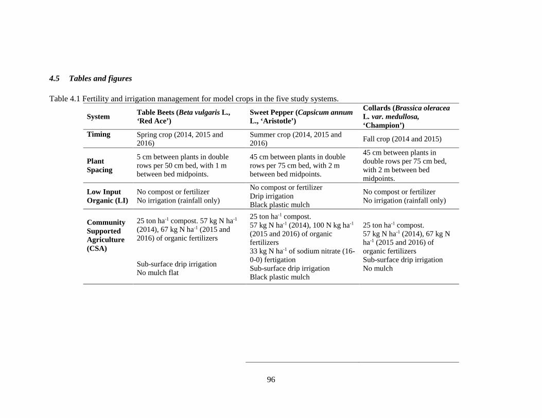
96
4.5 Tables and figures
Table 4.1 Fertility and irrigation management for model crops in the five study systems.
System Table Beets (Beta vulgaris L., ‘Red Ace’)
Sweet Pepper (Capsicum annum L., ‘Aristotle’)
Collards (Brassica oleracea L. var. medullosa, ‘Champion’)
Timing Spring crop (2014, 2015 and 2016)
Summer crop (2014, 2015 and 2016) Fall crop (2014 and 2015)
Plant Spacing
5 cm between plants in double rows per 50 cm bed, with 1 m between bed midpoints.
45 cm between plants in double rows per 75 cm bed, with 2 m between bed midpoints.
45 cm between plants in double rows per 75 cm bed, with 2 m between bed midpoints.
Low Input Organic (LI)
No compost or fertilizer No irrigation (rainfall only)
No compost or fertilizer Drip irrigation Black plastic mulch
No compost or fertilizer No irrigation (rainfall only)
Community Supported Agriculture (CSA)
25 ton ha-1 compost. 57 kg N ha-1 (2014), 67 kg N ha-1 (2015 and 2016) of organic fertilizers Sub-surface drip irrigation No mulch flat
25 ton ha-1 compost. 57 kg N ha-1 (2014), 100 N kg ha-1 (2015 and 2016) of organic fertilizers 33 kg N ha-1 of sodium nitrate (16-0-0) fertigation Sub-surface drip irrigation Black plastic mulch
25 ton ha-1 compost. 57 kg N ha-1 (2014), 67 kg N ha-1 (2015 and 2016) of organic fertilizers Sub-surface drip irrigation No mulch

97
Table 4.1 continued……………..
Movable High Tunnel system (MOV)
24 ton ha-1 horse manure compost 45 kg N ha-1 of pelleted organic fertilizer Drip irrigation Rainfall protection
24 ton ha-1 horse manure compost 45 kg N ha-1 of pelleted organic fertilizer 28 kg N ha-1 fertigation with liquid fish fertilizer Drip irrigation Rainfall protection
24 ton ha-1 horse manure compost 45 kg N ha-1 of pelleted organic fertilizer Drip irrigation Rainfall protection
Conventional system (CONV)
56 Kg N ha-1 balanced fertilizer at planting Drip irrigation
78 Kg N ha-1 balanced fertilizer at planting 60 kg N ha-1 calcium nitrate fertigation in split Drip irrigation Black plastic mulch
56 Kg N ha-1 balanced fertilizer at planting 60 kg N ha-1 calcium nitrate fertigation in split Drip irrigation Black plastic mulch
High Tunnel (HT)
24 ton ha-1 horse manure compost 45 kg N ha-1 of pelleted organic fertilizer Drip irrigation Rainfall protection
24 ton ha-1 horse manure compost 45 kg N ha-1 of pelleted organic fertilizer 28 kg N ha-1 fertigation with liquid fish fertilizer Drip irrigation Rainfall protection
24 ton ha-1 horse manure compost 45 kg N ha-1 of pelleted organic fertilizer Drip irrigation Rainfall protection

98
Table 4.2 Mean marketable (USDA grades 1&2) fresh yield of pepper, beet and collard from 2014, 2015 and 2016 in the five study systems. System Fresh crop yield (kg ha-1)
Beet Pepper Collard
LI 9,686±2350 19,637±806 3,524±356
CSA 30,681±2491 35,395±4427 25,819±1286
MOV 54,224±3972 56,130±3341 47,843±3634
CONV 28,933±4219 30,860±985 32,076±1126
HT 35,223±3642 44,936±3197 36,145±1864

99
Table 4.3 The averages soil NO3¯-N during pepper, beet and collard growing season from 2014, 2015, and 2016 in low input, community supported agriculture, movable high tunnel, conventional and high tunnel system
Average soil NO3¯-N (kg N ha-1)
Soil layer
(cm) System Beet Pepper Collard
LI 24 ± 1 66 ± 8 19 ± 4
CSA 31 ± 5 41 ± 7 7 ± 1
0-15 MOV 74 ± 6 67 ± 13 72 ± 21
CONV 23 ±3 44 ± 7 12 ± 3
HT 61 ± 5 72 ± 10 63 ± 10
LI 16 ± 0 25 ± 4 13 ± 2
CSA 14 ± 2 16 ± 2 15 ± 6
15-30 MOV 29 ± 5 15 ± 2 32 ± 13
CONV 14 ± 1 22 ± 3 5 ± 1
HT 21 ± 2 31 ± 8 19 ± 6
LI 14 ± 0 43 ± 6 14 ± 2
CSA 16 ± 1 21 ± 5 7 ± 2
30-50 MOV 38 ± 5 54 ± 11 48 ± 13
CONV 10 ± 1 27 ± 4 4 ± 0
HT 32 ± 3 53 ± 8 53 ± 10

100
Table 4.4 The Average crop N uptake and N fertilizer applied in five systems. System Beet Pepper Collard
N uptake
(kg N ha-1)
N applied
(kg N ha-1)
N uptake (kg
N ha-1)
N applied
(kg N ha-1)
N uptake
(kg N ha-1)
N applied
(kg N ha-1)
LI 41±10 0 107±2 0 13±1 0
CSA 115±9 167 164±16 200 74±3 167
MOV 171±8 145 240±12 201 179±13 145
CONV 100±22 56 148±3 138 120±4 116
HT 116±16 145 199±11 201 135±7 145

101
Figure 4.1 Overview of five model farming systems representing a gradient of intensification, as characterized by timing of production and fallow periods, tillage frequency, and nutrient inputs.

102
Figure 4.2 Mean NO3-N per lysimeter values in model crops in the five study systems from 2014, 2015 and 2016

103
CHAPTER 5. CONCLUSIONS
Chapters 2 and 3 of this dissertation quantified the soil mineral N dynamics, CO2
and N2O fluxes and characterize NO3¯ leaching from three different vegetable production
systems viz. low input organic system (LI), conventional system (CONV) and high tunnel
organic system (HT). Along with this, we calculated yield-scaled global warming
potential (GWP) for three vegetable production systems. Key loss pathways in the low
input (LI) system were via greenhouse gas fluxes, whereas in the conventional system
(CONV) they were via leaching. Although HT was expected to produce higher gas fluxes
due to greater soil mineral N content, this was not observed, although the peak timing and
basal flux patterns differed from the open field systems. Yield-scaled GWP was greater in
the LI system compared to CONV and HT system, driven both by greater fluxes as well
as lower yields. From the perspective of sustainable intensification in these three systems,
our study suggests CONV systems may benefit from reduced fertilizer inputs in
combination with irrigation management to minimize downward directed hydraulic
gradients particularly just after planting of crops; LI systems may benefit from targeted
additional fertilizer and irrigation inputs; and this work supports literature indicating the
need to examine long-term soil impacts in HT systems over longer timelines. These
results indicated that the soil mineral N content and N2O emission varied with vegetable
production systems with varied management practices. The N losses were high in LI,
although the total yield was not higher. Increasing the crop N uptake in LI system by
effectively managing weeds and targeted and timely irrigation might decrease the N2O
losses and N leaching, which was pronounced at the starting of cropping period.

104
However, such losses may be difficult to manage due to the nature of fallow conversion
to vegetable production.
In addition to this, RZWQM2 model was used to simulate soil water, N2O
emission, soil NO3¯-N processes and crop yield in diversified vegetable rotations
representing a gradient of production intensities. RZWQM2 simulated soil NO3¯-N
content reasonably well during beet, collard and bean growing seasons in CONV and LI
system, but could not simulate well during pepper crops which were grown under plastic
mulch. RZWQM2 simulated cumulative N2O emission from 2014 to 2016 was
reasonably well compared to field measured values in CONV system, while the model
overestimated in HT system and underestimated in LI system the cumulative N2O
emission. Crop yield and soil water content were simulated well in all systems. Overall,
this work contributes to key gaps in the literature characterizing environmental processes
contributing to evolution of sustainable intensification in vegetable production system.
The limitations in our study is lacking detail physiological crop growth parameters of
model crops for better simulation.

105
REFERENCES
Ahuja, L. R., K. W. Rojas, J. D. Hanson, M. J. Shaffer, and L. Ma, eds. 2000. The Root
Zone Water Quality Model. Highlands Ranch, Colo.: Water Resources
Publications.
Allaire-Leung, S.E., L. Wu, J.P. Mitchell and B.L. Sanden. 2001. Nitrate leaching and
soil nitrate content as affected by irrigation uniformity in a carrot field.
Agricultural Water Management 48: 37-50.
Barak, P., O.J. Babou, A.R. Krueger, L.A. Peterson and D.A. Laird. 1997. Effects of
long-term soil acidification due to nitrogen fertilizer inputs in Wisconsin. Plant
and Soil 197: 61–69.
Barbieri, P., S. Pellerin and T. Nesme. 2017. Comparing crop rotations between organic
and conventional farming. Scientific Reports 7: 13761.
Battye, R., W. Battye, C. Overcash and S. Fudge. 1994. Development and selection of
ammonia emissions factors. ED/R Incorporated, Durham, NC.
Benbi, D.K., A.K. Boparai and K. Brar. 2014. Decomposition of particulate organic
matter is more sensitive to temperature than the mineral associated organic matter.
Soil Biology and Biochemistry 70: 183-192.
Biernbaum J. 2013. Hoophouse Environment Management: Light, Temperature,
Ventilation. MSU Horticulture.
https://www.canr.msu.edu/hrt/uploads/535/78622/HT-LightTempManagement-
2013-10pgs.pdf (accessed on 9 Feb 2018).

106
Binkley, D. and P. Matson. 1983. Ion-exchange resin bag method for assessing forest
soil-nitrogen availability. Soil Science Society of America Journal 47(5), 1050-
1052.
Blatt, C.R. and K.B. McRae. 1998. Comparison of four organic amendments with a
chemical fertilizer applied to three vegetables in rotation. Canadian Journal of
Plant Science 78: 641-646.
Burney, J.A., S.J. Davis and D.B. Lobell. 2010. Greenhouse gas mitigation by
agricultural intensification. Proceedings of the National Academy of Sciences
107: 12052-12057.
Cameira, M.R., S. Tedesco and T.E. Leitao. 2014. Water and nitrogen budgets under
different production systems in Lisbon urban farming. Biosystems Engineering
125: 65-79.
Cassman, K.G. and D.N. Munns. 1980. Nitrogen Mineralization as Affected by Soil
Moisture, Temperature, and Depth. Soil Science Society of America Journal 44:
1233-1237.
Cassman K.G., Dobermann A., Walters D. 2002. Agroecosystems, nitrogen‐use
efficiency, and nitrogen management. Ambio 31: 132-140.
Chang, J., X. Wu, Y. Wang, L.A. Meyerson, B. Gu, Y. Min, H. Xue, C. Peng. 2013. Does
growing vegetables in plastic greenhouses enhance regional ecosystem services
beyond the food supply? Frontiers in Ecology and the Environment 11: 43-49.
Chen, H., X. Li, F. Hu and W. Shi. 2013. Soil nitrous oxide emissions following crop
residue addition: a meta-analysis. Global Change Biology 19: 2956-2964.

107
Cheng, Y., W. Xie, R. Huang, X. Yan and S. Wang. 2017. Extremely high N2O but
unexpectedly low NO emissions from a highly organic and chemical fertilized
peach orchard system in China. Agriculture, Ecosystems & Environment 246:
202-209.
Clark, M. and D. Tilman. 2017. Comparative analysis of environmental impacts of
agricultural production systems, agricultural input efficiency, and food choice.
Environmental Research Letters 12: 064016.
Cong, R., X. Wang, M. Xu, S.M. Ogle and W.J. Parton. 2014. Evaluation of the
CENTURY model using long-term fertilization trials under corn-wheat cropping
systems in the typical croplands of China. Plos One 9: e95142.
Congreves, K.A. and L.L. Van Eerd. 2015. Nitrogen cycling and management in
intensive horticultural systems. Nutrient Cycling in Agroecosystem 102: 299-318.
Creamer, N.G., and K.R. Baldwin. 2000. An evaluation of summer cover crops for use in
vegetable production systems in North Carolina. HortScience 35: 600–603.
Crowder, D.W. and J.P. Reganold. 2015. Financial competitiveness of organic agriculture
on a global scale. Proceedings of the National Academy of Sciences 112: 7611-
7616.
Crutchfield, J. D., and J.H. Grove. 2011. A new cadmium reduction device for the
microplate determination of nitrate in water, soil, plant tissue, and physiological
fluids. Journal of AOAC International 94: 1896-1905.
Cui, Z., S. Yue, G. Wang, F. Zhang and X. Chen. 2013. In-season root-zone N
management for mitigating greenhouse gas emission and reactive N losses in

108
intensive wheat production. Environmental Science & Technology 47: 6015-
6022.
Cui, Z., H. Zhang, X. Chen, C. Zhang, W. Ma, C. Huang, et al. 2018. Pursuing
sustainable productivity with millions of smallholder farmers. Nature 555: 363.
Darwish, T., T. Atallah, S. Hajhasan and A. Chranek. 2003. Management of nitrogen by
fertigation of potato in Lebanon. Nutrient Cycling in Agroecosystems 67: 1-11.
Davidson, E.A. and S.E. Trumbore. 1995. Gas diffusivity and production of CO2 in deep
soils of the eastern Amazon. Tellus B: Chemical and Physical Meteorology 47:
550-565.
Davidson, E.A., P.A. Matson, P.M. Vitousek, R. Riley, K. Dunkin, G. Garcia-Mendez
and J.M. Maass. 1993. Processes regulating soil emissions of NO and N2O in a
seasonally dry tropical forest. Ecology 74: 130-139.
Dawson, J.C., D.R. Huggins and S.S. Jones. 2008. Characterizing nitrogen use efficiency
in natural and agricultural ecosystems to improve the performance of cereal crops
in low-input and organic agricultural systems. Field Crops Research 107: 89-101.
de Ponti, T., B. Rijk and M.K. van Ittersum. 2012. The crop yield gap between organic
and conventional agriculture. Agricultural Systems 108: 1-9.
Del Grosso, S.J., W.J. Parton, A.R. Mosier, D.S. Ojima, A.E. Kulmala and S. Phongpan.
2000. General model for N2O and N2 gas emissions from soils due to
dentrification. Global Biogeochemical Cycles 14: 1045-1060.
Deng, J., Z. Zhou, X. Zheng and C. Li. 2013. Modeling impacts of fertilization
alternatives on nitrous oxide and nitric oxide emissions from conventional
vegetable fields in southeastern China. Atmospheric Environment 81: 642-650.

109
Dobbie, K.E. and K.A. Smith. 2003. Impact of different forms of N fertilizer on N2O
emissions from intensive grassland. Nutrient Cycling in Agroecosystems 67: 37-
46.
Dobbie, K.E., I.P. McTaggart and K.A. Smith. 1999. Nitrous oxide emissions from
intensive agricultural systems: Variations between crops and seasons, key driving
variables, and mean emission factors. Journal of Geophysical Research:
Atmospheres 104: 26891-26899.
Drinkwater, L.E. and S.S. Snapp. 2007. Nutrients in agroecosystems: Rethinking the
management paradigm. Advances in Agronomy 92: 163-186.
Dury, J., Schaller, N., Garcia, F., Reynaud, A., and J. E. Bergez. 2012. Models to support
cropping plan and crop rotation decisions: A review. Agronomy for Sustainable
Development 32(2): 567-580.
Engel T. and E. Priesack. 1993. Expert-N, a building block system How of nitrogen
models as a resource for advice, research, water management and policy. In:
Eijsackers H.J.P. and Hamers T. (eds), Integrated Soil and Sediment Research: A
Basis for Proper Protection. Kluwer Academic Publishers, Dordrecht, The
Netherlands, pp. 503–507.
Estavillo, J., P. Merino, M. Pinto, S. Yamulki, G. Gebauer, A. Sapek and W. Corre. 2002.
Short term effect of ploughing a permanent pasture on N2O production from
nitrification and denitrification. Plant and Soil 239: 253-265.
Evanylo, G., C. Sherony, J. Spargo, D. Starner, M. Brosius and K. Haering. 2008. Soil
and water environmental effects of fertilizer, manure, and compost-based fertility

110
practices in an organic vegetable cropping system. Agriculture, Ecosystems &
Environment 127: 50-58.
Fang, Q.X., L. Ma, A.D. Halvorson, R.W. Malone, L.R. Ahuja, S.J. Del Grosso and J.L.
Hatfield. 2015. Evaluating four nitrous oxide emission algorithms in response to
N rate on an irrigated corn field. Environmental Modelling & Software 72: 56-70.
Fang, Q.X., L. Ma, G.N. Flerchinger, Z. Qi, L.R. Ahuja, H.T. Xing, J. Li and Q. Yu.
2014. Modeling evapotranspiration and energy balance in a wheat–maize
cropping system using the revised RZ-SHAW model. Agricultural and Forest
Meteorology 194: 218-229.
FAO. 2011. The state of the world’s land and water resources for food and agriculture
(SOLAW) – Managing systems at risk. Food and Agriculture Organization of the
United Nations, Rome and Earthscan, London.
FAOSTAT. 2018. Crops data. http://www.fao.org/faostat/en/#data/QC/visualize . fao.org.
FAO. (accessed 12 April 2018)
Feaga, J.B., J.S. Selker, R.P. Dick and D.D. Hemphill. 2010. Long-term nitrate leaching
under vegetable production with cover crops in the pacific northwest. Soil Science
Society of America Journal 74: 186-195.
Feng, G., H. Tewolde, L. Ma, A. Adeli, K.R. Sistani and J.N. Jenkins. 2015. Simulating
the fate of fall- and spring-applied poultry litter nitrogen in corn production. Soil
Science Society of America Journal 79: 1804.
Fernandez, M.D., A.M. Gonzalez, J. Carreno, C. Perez and S. Bonachela. 2007. Analysis
of on-farm irrigation performance in Mediterranean greenhouses. Agricultural
Water Management 89: 251-260.
111
Flerchinger, G.N. and K.E. Saxton. 1989. Simultaneous heat and water model of a
freezing snow-residue-soil system. I. Theory and development. Transactions of
the American Society of Agricultural Engineers 32: 565-571.
Foley, J.A., N. Ramankutty, K.A. Brauman, E.S. Cassidy, J.S. Gerber, M. Johnston, et al.
2011. Solutions for a cultivated planet. Nature 478: 337-342.
Forster, P., V. Ramaswamy, P. Artaxo, T. Berntsen, R. Betts and D.W. Fahey. 2007.
Changes in atmospheric constituents and in radiative forcing. In: Solomon, S.,
Qin, D., Manning, M., Chen, Z., Marquis, M., Averyt, K.B., Tignor, M., Miller,
H.L. (Eds.), Climate change (2007): The physical science basis. Contribution of
Working Group I to the Fourth Assessment Report of the Intergovernmental Panel
on Climate Change. Cambridge University Press, Cambridge, pp. 212.
Franzluebbers, A.J., J. Sawchik and M.A. Taboada. 2014. Agronomic and environmental
impacts of pasture–crop rotations in temperate North and South America.
Agriculture, Ecosystems & Environment 190: 18-26.
Gallardo, M., C. Gimenez, C. Martínez-Gaitan, C.O. Stockle, R.B. Thompson and M.R.
Granados. 2011. Evaluation of the VegSyst model with muskmelon to simulate
crop growth, nitrogen uptake and evapotranspiration. Agricultural Water
Management 101: 107-117.
Gallardo, M., M.D. Fernandez, C. Gimenez, F.M. Padilla and R.B. Thompson. 2016.
Revised VegSyst model to calculate dry matter production, critical N uptake and
ETc of several vegetable species grown in Mediterranean greenhouses.
Agricultural Systems 146: 30-43.

112
Galloway, J.N., F.J. Dentener, D.G. Capone, E.W. Boyer, R.W. Howarth, S.P. Seitzinger,
et al. 2004. Nitrogen cycles: past, present, and future. Biogeochemistry 70: 153-
226.
Garbach, K., J. C. Milder, F. A. J. DeClerck, M. Montenegro de Wit, L. Driscoll and B.
Gemmill-Herren. 2016. Examining multi-functionality for crop yield and
ecosystem services in five systems of agroecological intensification. International
Journal of Agricultural Sustainability15(1): 11-28.
Garcia-Prechac, F., O. Ernst, G. Siri-Prieto and J.A. Terra. 2004. Integrating no-till into
crop–pasture rotations in Uruguay. Soil and Tillage Research 77: 1-13.
Gary, C., J.W. Jones and M. Tchamitchian. 1998. Crop modelling in horticulture: State of
the art. Scientia Horticulturae 74: 3-20.
Gaskell, M. and R. Smith. 2007. Nitrogen sources for organic vegetable crops.
HortTechnology 17: 431-441.
Gillette, K., L. Ma, R.W. Malone, Q.X. Fang, A.D. Halvorson, J.L. Hatfield and L.R.
Ahuja. 2017. Simulating N2O emissions under different tillage systems of
irrigated corn using RZ-SHAW model. Soil and Tillage Research 165: 268-278.
Gillette, K., R.W. Malone, T.C. Kaspar, L. Ma, T.B. Parkin, D.B. Jaynes, Q.X. Fang, J.L.
Hatfield, G.W. Feyereisen and K.C. Kersebaum. 2018. N loss to drain flow and
N2O emissions from a corn-soybean rotation with winter rye. Science of The
Total Environment 618: 982-997.
Gliessman, S.R. 2007. Agroecology: The ecology of sustainable food systems. 2nd CRC
Press, Taylor & Francis group.

113
Goulding, K. 2000. Nitrate leaching from arable and horticultural land. Soil Use and
Management 16: 145-151.
Grant, R.F. and E. Pattey. 1999. Mathematical modeling of nitrous oxide emissions from
an agricultural field during spring thaw. Global Biogeochemical Cycles 13: 679-
694.
Grassini, P. and K.G. Cassman. 2012. High-yield maize with large net energy yield and
small global warming intensity. Proceedings of the National Academy of Sciences
109: 1074-1079.
Guo, R., W. Qin, C. Jiang, L. Kang, C. Nendel and Q. Chen. 2018. Sweet corn
significantly increases nitrogen retention and reduces nitrogen leaching as
summer catch crop in protected vegetable production systems. Soil and Tillage
Research 180: 148-153.
Han, Z., M. T. Walter and L. E. Drinkwater. 2017. N2O emissions from grain cropping
systems: a meta-analysis of the impacts of fertilizer-based and ecologically-based
nutrient management strategies. Nutrient Cycling Agroecosystem 107: 335–355.
Hanselman, T.A., D.A. Graetz and T.A. Obreza. 2004. A comparison of in situ methods
for measuring net nitrogen mineralization rates of organic soil amendments.
Journal Environment Quality 33: 1098-1105.
Haynes, R.J., R.S. Swift and R.C. Stephen .1991. Influence of mixing cropping rotation
(pasture arable) on organic matter content, water stable aggregation and clod
porosity of soils. Soil and Tillage Research 19: 77-79.
114
He, F., Q. Chen, R. Jiang, X. Chen, F. Zhang. 2007. Yield and nitrogen balance of
greenhouse tomato (Lycopersicum esculentum Mill.) with conventional and site-
specific nitrogen management in northern China. Nutrient Cycling in
Agroecosystems 77: 1-14.
Henault, C., F. Bizouard, P. Laville, B. Gabrielle, B. Nicoullaud, J.C. Germon and P.
Cellier. 2005. Predicting in situ soil N2O emission using NOE algorithm and soil
database. Global Change Biology 11: 115-127.
IPCC. 2007. Changes in atmospheric constituents and in radiative forcing. In: Solomon,
S., D. Qin, M. Manning, Z. Chen, M. Marquis, K.B. Averyt, M. Tignor and H.L.
Miller (eds.), Climate Change 2007: The Physical Science Basis. Cambridge
University Press, Cambridge, UK.
Iqbal, J., J.A. Nelson and R.L. McCulley. 2013. Fungal endophyte presence and genotype
affect plant diversity and soil-to-atmosphere trace gas fluxes. Plant and Soil 364:
15-27.
Jamali, H., W. Quayle, C. Scheer and J. Baldock. 2016. Mitigation of N2O emissions
from surface-irrigated cropping systems using water management and the
nitrification inhibitor DMPP. Soil Research 54: 481-493.
Jiang, Q., Z. Qi, C.A. Madramootoo and C. Creze. 2019. Mitigating greenhouse gas
emissions in subsurface-drained field using RZWQM2. Science of the Total
Environment 646: 377-389.
Johnson, D.W., P.S.J. Verburg and J.A. Arnone. 2005. Soil extraction, ion exchange
resin, and ion exchange membrane measures of soil mineral nitrogen during

115
incubation of a tallgrass prairie soil. Soil Science Society of America Journal 69:
260-265.
Ju, X.T., C.L. Kou, P. Christie, Z.X. Dou and F.S. Zhang. 2007. Changes in the soil
environment from excessive application of fertilizers and manures to two
contrasting intensive cropping systems on the North China Plain. Environmental
Pollution 145: 497-506.
Khalil, K., B. Mary and P. Renault. 2004. Nitrous oxide production by nitrification and
denitrification in soil aggregates as affected by O2 concentration. Soil Biology and
Biochemistry 36: 687-699.
Kim, Y., S. Berger, J. Kettering, J. Tenhunen, E. Haas and R. Kiese. 2014. Simulation of
N2O emissions and nitrate leaching from plastic mulch radish cultivation with
Landscape DNDC. Ecological Research 29: 441-454.
Knapp, S. and M.G.A. van der Heijden. 2018. A global meta-analysis of yield stability in
organic and conservation agriculture. Nature Communications 9: 3632.
Knewtson, S.J.B., M.B. Kirkham, R.R. Janke, L.W. Murray and E.E. Carey. 2012. Soil
quality after eight years under high tunnels. HortScience 47: 1630-1633.
Kniss, A.R., S.D. Savage and R. Jabbour. 2016. Commercial crop yields reveal strengths
and weaknesses for organic agriculture in the United States. Plos One 11:
e0161673.
Kolberg, R. L., D.G. Westfall and G.A. Peterson. 1999. Influence of cropping intensity
and nitrogen fertilizer rates on in situ nitrogen mineralization. Soil Science
Society of America Journal 63(1): 129-134.

116
Kraft, G.J. and W. Stites. 2003. Nitrate impacts on groundwater from irrigated-vegetable
systems in a humid north-central US sand plain. Agriculture, Ecosystems &
Environment 100: 63-74.
Kramer, S.B., J.P. Reganold, J.D. Glover, B.J.M. Bohannan and H.A. Mooney. 2006.
Reduced nitrate leaching and enhanced denitrifier activity and efficiency in
organically fertilized soils. Proceedings of the National Academy of Sciences of
the United States of America 103: 4522-4527.
Kravchenko, A.N., E.R. Toosi, A.K. Guber, N.E. Ostrom, J. Yu, K. Azeem, M.L. Rivers
and G.P. Robertson. 2017. Hotspots of soil N2O emission enhanced through water
absorption by plant residue. Nature Geoscience 10: 496-500.
Kusa K., T. Sawamoto and R. Hatano. 2002. Nitrous oxide emissions for 6 years from a
gray lowland soil cultivated with onions in Hokkaido, Japan. Nutrient Cycling in
Agroecosystems 63: 239-247.
KYMESONET. 2018. KENTUCKY MESONET weather data.
http://www.kymesonet.org/ (accessed 1 Feb 2017).
Lament, W.J. 1993. Plastic mulches for the production of vegetable crops.
HortTechnology 3: 35-39.
Leikam D.F. and R.E. Lamond. 2003. Estimating manure nutrient availability. Kansas
State University Agricultural Experiment Station and Cooperative Extension
Service. http://agprofessional.com/sites/default/files/MF2562.pdf (Accessed on 8
Nov 2018).

117
Li, C., S. Frolking and T.A. Frolking. 1992. A model of nitrous oxide evolution from soil
driven by rainfall events: 1. Model structure and sensitivity. Journal of
Geophysical Atmospheres 97: 9759-9776.
Li, Y., R. White, D. Chen, J. Zhang, B. Li, Y. Zhang, et al. 2007. A spatially referenced
water and nitrogen management model (WNMM) for (irrigated) intensive
cropping systems in the North China Plain. Ecological Modelling 203: 395-423.
Liebman, M. and A.S. Davis. 2000. Integration of soil, crop and weed management in
low-external-input farming systems. Weed Research 40: 27-47.
Liptzin D. and R. Dahlgren. 2016. A California nitrogen mass balance for 2005. In T.P.
Tomich, S.B. Brodt, R.A. Dahlgren and K.M. Scow (Eds.), The California
Nitrogen Assessment (79-112). California: University of California Press.
Loick, N., E. Dixon, D. Abalos, A. Vallejo, P. Matthews, K. McGeough, E.M. Baggs and
L.M. Cardenasa. 2017. “Hot spots” of N and C impact nitric oxide, nitrous oxide
and nitrogen gas emissions from a UK grassland soil. Geoderma 305: 336-345.
Lokupitiya, E. and K. Paustian. 2006. Agricultural soil greenhouse gas emissions: a
review of national inventory methods. Journal of Environmental Quality 35:
1413-1427.
Ma, L., L. Ahuja, B.T. Nolan, R. Malone, T. Trout and Z. Qi. 2012. Root zone water
quality model (RZWQM2): Model use, calibration and validation. Transactions of
the American Society of Agricultural and Biological Engineers 55: 1425-1446.
Ma, L., R.W. Malone, P. Heilman, D.L. Karlen, R.S. Kanwar, C.A. Cambardella, S.A.
Saseendran and L.R. Ahuja. 2007. RZWQM simulation of long-term crop

118
production, water and nitrogen balances in Northeast Iowa. Geoderma 140: 247-
259.
Malone, R.W., L.R. Ahuja, L. Ma, R.D. Wauchope, Q. Ma and K.W. Rojas. 2004.
Application of the Root Zone Water Quality Model (RZWQM) to pesticide fate
and transport: An overview. Pest Management Science 60: 205-221.
Matson, P.A., W.J. Parton, A.G. Power and M.J. Swift. 1997. Agricultural intensification
and ecosystem properties. Science 277: 504-509.
McCarty, G., and J. Meisinger. 1997. Effects of N fertilizer treatments on biologically
active N pools in soils under plow and no tillage. Biology and Fertility of
Soils, 24(4): 406-412.
Millar, N., A. Urrea, K. Kahmark, I. Shcherbak, G.P. Robertson and I. Ortiz-Monasterio.
2018. Nitrous oxide (N2O) flux responds exponentially to nitrogen fertilizer in
irrigated wheat in the Yaqui Valley, Mexico. Agriculture, Ecosystems &
Environment 261: 125-132.
Mohler, C. and S.E. Johnson. 2009. Crop rotation on organic farms a planning manual.
Natural Resource, Agriculture and Engineering Service. www.sare.org/Learning-
Center/Books/Crop-Rotation-on-Organic-Farms. (accessed 12 March 2017).
Monterroso, V.A. and H.C. Wien. 1990. Flower and pod abscission due to heat stress in
beans. Journal of the American Society for Horticultural Science 115: 631-634.
Montri, A. and J. Biernbaum. 2009. Management of the soil environment in high tunnels.
HortTechnology 19:34–36.
Mueller, N.D., J.S. Gerber, M. Johnston, D.K. Ray, N. Ramankutty and J.A. Foley. 2012.
Closing yield gaps through nutrient and water management. Nature 490: 254.
119
Muramoto, J., R.F. Smith, C. Shennan, K.M. Klonsky, J. Leap, M.S. Ruiz and S.R.
Gliessman. 2011. Nitrogen contribution of legume/cereal mixed cover crops and
organic fertilizers to an organic broccoli crop. HortScience 46: 1154-1162.
Nair, A., and K. Delate. 2016. Composting, crop rotation, and cover crop practices in
organic vegetable production. In D. Nandwani (Ed.), Organic Farming for
Sustainable Agriculture, 9: 231-257.
Neeteson, J.J. and O.T. Carton. 2001. The environmental impact of nitrogen in field
vegetable production. Acta Horticulture 563: 21-28.
NOAA. 2018. National Weather Service. https://www.weather.gov/ (accessed 1 Feb
2017).
Norris, C.E. and K.A. Congreves. 2018. Alternative management practices improve soil
health indices in intensive vegetable cropping systems: a review. Frontiers in
Environmental Science 6: 1-18.
Norse, D. and X. Ju. 2015. Environmental costs of China’s food security. Agriculture,
Ecosystems & Environment 209: 5-14.
Norse, D., Y. Lu and J. Huang. 2014. China’s food security: is it a national, regional or
global issue? China and the EU in context: insights for business and investors.
Palgrave Macmillan UK, London, pp. 251-302.
Olesen, J.E., B.M. Petersen, J. Berntsen, S. Hansen, P.D. Jamieson and A.G. Thomsen.
2002. Comparison of methods for simulating effects of nitrogen on green area
index and dry matter growth in winter wheat. Field Crops Research 74: 131-149.

120
Parkin, T.B., J.W Doran and E. Franco-Vizcaino. 1996. Field and laboratory tests of soil
respiration. In: J.W., D., Jones, A.J. (Eds.), Methods for assessing soil quality,
Madison, WI, pp. 231–245.
Parkin, T.B., Venterea, R.T., 2010. Chapter 3: Chamber-based trace gas flux
measurements. In: R.F. Follett (Ed.), GRACEnet Sampling protocols, USDA-
ARS, Fort Collins, CO, pp. 3-39.
Parton, W.J., E.A. Holland, S.J. Del Grosso, M.D. Hartman, R.E. Martin, A.R. Mosier,
D.S. Ojima, D.S. Schimel. 2001. Generalized model for NOx and N2O emissions
from soils. Journal of Geophysical Research 106: 17403–17420.
Parton, W.J., M. Hartman, D. Ojima and D. Schimel. 1998. DAYCENT and its land
surface submodel: description and testing. Global and Planetary Change 19: 35-
48.
Pinto, M., P. Merino, A. del Prado, J.M. Estavillo, S. Yamulki, G. Gebauer, S. Piertzak, J.
Lauf and O. Oenema. 2004. Increased emissions of nitric oxide and nitrous oxide
following tillage of a perennial pasture. Nutrient Cycling in Agroecosystems 70:
13-22.
Ponisio, L.C., L.K. M'Gonigle, K.C. Mace, J. Palomino, P. de Valpine and C. Kremen.
2015. Diversification practices reduce organic to conventional yield gap.
Proceedings of the Royal Society B: Biological Sciences 282: 20141396.
Poudel, D.D., W.R. Horwath, W.T. Lanini, S.R. Temple and A.H.C. van Bruggen. 2002.
Comparison of soil N availability and leaching potential, crop yields and weeds in
organic, low-input and conventional farming systems in northern California.
Agriculture, Ecosystems & Environment 90: 125-137.
121
Powell, M., B. Gundersen, J. Cowan, C.A. Miles and D.A. Inglis. 2014. The effect of
open-ended high tunnels in western Washington on late blight and physiological
leaf roll among five tomato cultivars. Plant Disease 98: 1639-1647.
Pradhan, P., G. Fischer, H. van Velthuizen, D.E. Reusser and J.P. Kropp. 2015. Closing
yield gaps: How sustainable can we be? Plos One 10: e0129487.
Pretty, J. 2008. Agricultural sustainability: Concepts, principles and evidence.
Philosophical Transactions of the Royal Society B: Biological Sciences 363: 447-
465.
Pretty, J.N. 1997. The sustainable intensification of agriculture. Natural Resources Forum
21: 247-256.
Quan, Z., B. Huang, C. Lu, Y. Shi, Y. Cao, Y. Wang, C. He, G. Chi, J. Ma and X. Chen.
2015. Nitrogen accumulation and loss in a high-input greenhouse vegetable
cropping system elevated by application of manures. HortScience 50: 1688-1693.
Reeve, J. and D. Drost. 2012. Yields and soil quality under transition organic high tunnel
tomatoes. HortScience 47:38–44.
Rezaei Rashti, M., W. Wang, P. Moody, C. Chen and H. Ghadiri. 2015. Fertilizer-
induced nitrous oxide emissions from vegetable production in the world and the
regulating factors: A review. Atmospheric Environment 112: 225-233.
Rice, C.W. and M.S. Smith. 1984. Short-term immobilization of fertilizer nitrogen at the
surface of no-till and plowed soils. Soil Science Society of America Journal 48:
295-297.
122
Robacer, M., S. Canali, H.L. Kristensen, F. Bavec, S.G. Mlakar, M. Jakop and M. Bavec.
2016. Cover crops in organic field vegetable production. Scientia Horticulturae
208: 104-110.
Robertson, G.P. and S.M. Swinton. 2005. Reconciling agricultural productivity and
environmental integrity: a grand challenge for agriculture. Frontiers in Ecology
and the Environment 3: 38-46.
Rosenstock T.S and T.P. Tomich. 2016. Direct drivers of California’s nitrogen cycle. In
T.P. Tomich, S.B. Brodt, R.A. Dahlgren and K.M. Scow (Eds.), The California
Nitrogen Assessment (45-77). California: University of California Press.
Sainju, U.M., W.B. Stevens, T. Caesar-TonThat and M.A. Liebig. 2012. Soil greenhouse
gas emissions affected by irrigation, tillage, crop rotation, and nitrogen
fertilization. Journal of Environmental Quality 41: 1774-1786.
Schaufler, G., B. Kitzler, A. Schindlbacher, U. Skiba, M.A. Sutton and S. Zechmeister-
Boltenstern. 2010. Greenhouse gas emissions from European soils under different
land use: effects of soil moisture and temperature. European Journal of Soil
Science 61: 683-696.
Schellenberg, D.L., M.M. Alsina, S. Muhammad, C.M. Stockert, M.W. Wolff, B.L.
Sanden, P.H. Brown and D.R. Smart. 2012. Yield-scaled global warming
potential from N2O emissions and CH4 oxidation for almond (Prunus dulcis)
irrigated with nitrogen fertilizers on arid land. Agriculture, Ecosystems &
Environment 155: 7-15.
123
Schrama, M., J.J. de Haan, M. Kroonen, H. Verstegen and W.H. Van der Putten. 2018.
Crop yield gap and stability in organic and conventional farming systems.
Agriculture, Ecosystems & Environment 256: 123-130.
Sehy, U., R. Ruser and J.C. Munch. 2003. Nitrous oxide fluxes from maize fields:
relationship to yield, site-specific fertilization, and soil conditions. Agriculture,
Ecosystems & Environment 99: 97-111.
Seufert, V., N. Ramankutty and J.A. Foley. 2012. Comparing the yields of organic and
conventional agriculture. Nature 485: 229-232.
Shelton, R.E., K.L. Jacobsen and R.L. McCulley. 2018. Cover crops and fertilization alter
nitrogen loss in organic and conventional conservation agriculture systems.
Frontiers in Plant Science 1-8.
Shennan, C. 1992. Cover crops, nitrogen cycling, and soil properties in semi-irrigated
vegetable production systems. Hort Science 27:749-754.
Shi, W.-M., J. Yao and F. Yan. 2009. Vegetable cultivation under greenhouse conditions
leads to rapid accumulation of nutrients, acidification and salinity of soils and
groundwater contamination in South-Eastern China. Nutrient Cycling in
Agroecosystems 83: 73-84.
Shrestha D., O. Wendroth and K.L. Jacobsen. 2018. Nitrogen loss and greenhouse gas
flux across an intensification gradient in diversified vegetable rotations.
Manuscript submitted for publication.
Singandhupe, R.B., G.G.S.N. Rao, N.G. Patil and P.S. Brahmanand. 2003. Fertigation
studies and irrigation scheduling in drip irrigation system in tomato crop
(Lycopersicon esculentum L.). European Journal of Agronomy 19: 327-340.

124
Spiegal, S., B.T. Bestelmeyer, D.W. Archer, D.J. Augustine, E.H. Boughton, R.K.
Boughton, et al. 2018. Evaluating strategies for sustainable intensification of US
agriculture through the Long-Term Agroecosystem Research network.
Environmental Research Letters 13: 034031.
Stefanelli, D., I. Goodwin and R. Jones. 2010. Minimal nitrogen and water use in
horticulture: Effects on quality and content of selected nutrients. Food Research
International 43: 1833-1843.
Susfalk, R.B. and D.W. Johnson. 2002. Ion exchange resin based soil solution lysimeters
and snowmelt solution collectors. Communications in Soil Science and Plant
Analysis 33: 1261-1275.
Tei, F., A. Scaife and D.P. Aikman. 1996. Growth of lettuce, onion, and red beet. 1.
growth analysis, light interception, and radiation use efficiency. Annals of Botany
78: 633-643.
Thorup-Kristensen, K., J. Magid and L.S. Jensen. 2003. Catch crops and green manures
as biological tools in nitrogen management in temperate zones. Advances in
Agronomy 79: 227-302.
Tian, D., Y. Zhang, Y. Mu, Y. Zhou, C. Zhang and J. Liu. 2017. The effect of drip
irrigation and drip fertigation on N2O and NO emissions, water saving and grain
yields in a maize field in the North China Plain. Science of The Total
Environment 575: 1034-1040.
Tilman, D., C. Balzer, J. Hill and B.L. Befort. 2011. Global food demand and the
sustainable intensification of agriculture. Proceedings of the National Academy of
Sciences 108: 20260-20264.

125
UK Cooperative Extension Service. 2014. ID-36 Vegetable production guide for
commercial growers. University of Kentucky College of Agriculture, Food and
Environment Cooperative Extension Service.
USDA NASS. 2011. Agricultural chemical use: Vegetable crops 2010.
https://www.nass.usda.gov/Surveys/Guide_to_NASS_Surveys/Chemical_Use/Ve
getableChemicalUseFactSheet.pdf
USDA NASS. 2014. Census of horticultural specialties (2014). USDA NASS, 3(3): 508-
514.
https://www.agcensus.usda.gov/Publications/2012/Online_Resources/Census_of_
Horticulture_Specialties/HORTIC.pdf
USDA, 2018. National Organic Program Handbook: Guidance and instructions for
accredited certifying agents and certified operations. USDA National Organic
Program, Washington, US.
https://www.ams.usda.gov/sites/default/files/media/Program%20Handbk_TOC.pd
f (accessed on 9 Sept 2018).
Uzoma, K.C., W. Smith, B. Grant, R.L. Desjardins, X. Gao, K. Hanis, M. Tenuta, P.
Goglio and C. Li. 2015. Assessing the effects of agricultural management on
nitrous oxide emissions using flux measurements and the DNDC model.
Agriculture, Ecosystems & Environment 206: 71-83.
Uzun, S. and H. Kar. 2004. Quantitative effects of planting time on vegetative growth
of broccoli (Brassica oleracea var. italica). Pakistan Journal of Botany
36(4):769–777.

126
van Genuchten. 1980. A closed-form equation for predicting the hydraulic conductivity
of unsaturated soils. Soil Science Society of America Journal 44: 892-896.
van Genuchten, M. Th., F. J. Leij, and S. R. Yates. 1991. The RETC code for quantifying
the hydraulic functions of unsaturated soils, Version 1.0. EPA Report 600/2-
91/065, U.S. Salinity Laboratory, USDA-ARS, Riverside, California.
Venterea, R.T., B. Maharjan and M.S. Dolan. 2011. Fertilizer source and tillage effects
on yield-scaled nitrous oxide emissions in a corn cropping system. Journal of
Environmental Quality 40: 1521-1531.
Wang, X., C. Zou, X. Gao, X. Guan, Y. Zhang, X. Shi, X. Chen. 2018. Nitrate leaching
from open-field and greenhouse vegetable systems in China: A meta-analysis.
Environmental Science and Pollution Research 25: 31007-31016.
Wang, Z., Z. Qi, L. Xue and M. Bukovsky. 2016. RZWQM2 simulated management
practices to mitigate climate change impacts on nitrogen losses and corn
production. Environmental Modelling & Software 84: 99-111.
Web Soil Survey .2018. USDA NRCS Web Soil Survey.
https://websoilsurvey.sc.egov.usda.gov/App/HomePage.htm (accessed 1 April
2017).
Weinberger, K. and T.A. Lumpkin. 2007. Diversification into horticulture and poverty
reduction: A research agenda. World Development 35: 1464-1480.
Wells, A.T., K.Y. Chan and P.S. Cornish. 2000. Comparison of conventional and
alternative vegetable farming systems on the properties of a yellow earth in New
South Wales. Agriculture, Ecosystems & Environment 80: 47-60.

127
Wezel, A., G. Soboksa, S. McClelland, F. Delespesse and A. Boissau. 2015. The blurred
boundaries of ecological, sustainable, and agroecological intensification: a
review. Agronomy for Sustainable Development 35: 1283-1295.
Xu, X., Y. Ran, Y. Li, Q. Zhang, Y. Liu, H. Pan, X. Guan, J. Li, J. Shi, L. Dong, Z. Li, H.
Di and J. Xu. 2016. Warmer and drier conditions alter the nitrifier and denitrifier
communities and reduce N2O emissions in fertilized vegetable soils. Agriculture,
Ecosystems & Environment 231: 133-142.
Yaghi, T., A. Arslan and F. Naoum. 2013. Cucumber (Cucumis sativus, L.) water use
efficiency (WUE) under plastic mulch and drip irrigation. Agricultural Water
Management 128: 149-157.
Yu, Q., S.A. Saseendran, L. Ma, G.N. Flerchinger, T.R. Green and L.R. Ahuja. 2006.
Modeling a wheat–maize double cropping system in China using two plant
growth modules in RZWQM. Agricultural Systems 89: 457-477.
Zebarth, B.J., S. Freyman and C.G. Kowalenko. 1991. Influence of nitrogen fertilization
on cabbage yield, head nitrogen content and extractable soil inorganic nitrogen at
harvest. Canadian Journal of Plant Science 71: 1275-1280.
Zhang, J., H. Li, Y. Wang, J. Deng and L. Wang. 2018. Multiple-year nitrous oxide
emissions from a greenhouse vegetable field in China: Effects of nitrogen
management. Science of The Total Environment 616-617: 1139-1148.
Zhang, Y., F. Lin, Y. Jin, X. Wang, S. Liu and J. Zou. 2016. Response of nitric and
nitrous oxide fluxes to N fertilizer application in greenhouse vegetable cropping
systems in southeast China. Scientific Reports 6: 20700.

128
Zhang, Y.L., F.X. Wang, C.C. Shock, K.J. Yang, S.Z. Kang, J.T. Qin and S. Li. 2017.
Influence of different plastic film mulches and wetted soil percentages on potato
grown under drip irrigation. Agricultural Water Management 180: 160-171.
Zhou, X., L. Zhou, Y. Nie, Y. Fu, Z. Du, J. Shao, Z. Zheng and X. Wang. 2016. Similar
responses of soil carbon storage to drought and irrigation in terrestrial ecosystems
but with contrasting mechanisms: A meta-analysis. Agriculture, Ecosystems &
Environment 228: 70-81.
Zhu, J.H., X.L. Li, P. Christie and J.L. Li. 2005. Environmental implications of low
nitrogen use efficiency in excessively fertilized hot pepper (Capsicum frutescens
L.) cropping systems. Agriculture, Ecosystems & Environment 111: 70-80.
Zikeli, S., L. Deil and K. Moller. 2017. The challenge of imbalanced nutrient flows in
organic farming systems: A study of organic greenhouses in Southern Germany.
Agriculture, Ecosystems & Environment 244: 1-13.
Zurovec, O., B.K. Sitaula, H. Custovic, J. Zurovec and P. Dorsch. 2017. Effects of tillage
practice on soil structure, N2O emissions and economics in cereal production
under current socio-economic conditions in central Bosnia and Herzegovina. Plos
One 12: 1-22.
129
VITA
Debendra Shrestha
Education
Graduate Certificate (Applied Statistics), University of Kentucky, 2016 M.Sc. Ag (Horticulture), Tribhuvan University, Nepal, 2011. B.Sc. Agriculture, Tribhuvan University, Nepal, 2009.
Professional Positions
• Graduate Research Assistant, Department of Horticulture, Tribhuvan University from 2009 to 2011.
• Agriculture Extension Officer, Department of Agriculture/Ministry of Agriculture Development/ Government of Nepal, 2011-2014.
• Graduate Research Assistant, University of Kentucky, 2014 -2018. Publications
• Shrestha, D. 2013. Indigenous vegetables of Nepal for biodiversity and food security. International Journal of Biodiversity and Conservation, 5(3), 98-108.
• Shrestha, D., A. Srivastava, S.M. Shakya, J. Khadka and B.S Acharya. 2012.
Use of compost supplemented human urine in sweet pepper (Capsicum annuum L.) production. Scientia Horticulture, 153:8-12.
• Khadka, J. and D. Shrestha. 2012. Plant dry matter production and partitioning
of sour lime saplings fertilized with human urine. Nepalese Horticulture, 8:29-34.
Honors and Awards
• Awarded with University merit scholarship by Institute of Agriculture and Animal Science/Tribhuvan University in Bachelor of Agriculture and in Masters in Horticulture.
• International Nitrogen Initiative 2016 Travel Award


