
The multiple faces of shrinkageGeorg HeinzeCenter for Medical Statistics, Informatics and Intelligent SystemsSection for Clinical [email protected]
Partly supported by Austrian Science Fund FWF, Project I2276-N33

The multiple faces of shrinkage
•
•
Dunkler, Sauerbrei and Heinze, JStatSoft 2016
•
Puhr, Heinze, Nold, Lusa and Geroldinger, StatMed 2017

Historical outline
•
•
•
•
•
•
•
•
•

Purposes of shrinkage estimators
•
•
•
•

Post-estimation shrinkage methodsJoint work with Michael Kammer, Daniela Dunkler, Willi Sauerbrei


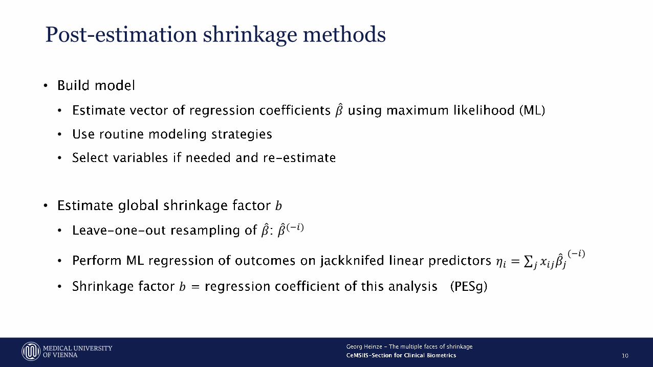
Post-estimation shrinkage methods
•
• 𝛽
•
•
• 𝑏
• 𝛽 𝛽(−𝑖)
• 𝜂𝑖 = 𝑗 𝑥𝑖𝑗 𝛽𝑗
(−𝑖)
• 𝑏

Use of the shrinkage factors
•
•
•
•
•
•
𝑦𝑛𝑒𝑤 = 𝛽0 + 𝑏 𝑥𝑖𝑛𝑒𝑤 𝛽
•

Sauerbrei‘s (1999) ‚parameterwise shrinkage factors‘
• 𝛽 𝛽(−𝑖)
•
partial 𝜂𝑖𝑗 = 𝑥𝑖𝑗 𝛽𝑗(−𝑖)
• 𝑏𝑗
•

Dunkler‘s (2016) extension of parameterwise shrinkage
• 𝑏𝑗
•
•
•
•
• 𝐺 𝜂𝑖𝑔 = 𝑗∈𝐽𝑔𝑥𝑖𝑗
𝛽𝑗(−𝑖)
𝑔 = 1, … , 𝐺
• 𝜂𝑖𝑔 𝑏𝑔, 𝑔 = 1, … , 𝐺
• 𝛽(−𝑖) ≈ 𝛽 − 𝐷𝐹𝐵𝐸𝑇𝐴𝑖

Example: deep vein thrombosis study

How do shrinkage effects of different methods compare?
•
•
•
• 𝜆
• 𝜆
•
•
•
•


too pessimistic
too optimistic


From bias reduction to shrinkage and beyondJoint work with Rainer Puhr, Angelika Geroldinger, Sander Greenland

Setting the scene
𝛽
𝛽
𝜋
𝜋
𝛽 𝜋

Firth‘s penalization for logistic regression
𝐿∗ 𝛽 = 𝐿 𝛽 det( 𝐼 𝛽 )1/2,
𝐼 𝛽 𝐿 𝛽
• 𝛽,
•
•

Firth‘s penalization for logistic regression
𝐿∗ 𝛽 = 𝐿 𝛽 det(𝑋𝑡𝑊𝑋)1/2
𝑊 = diag expit Xi𝛽 (1 − expit Xi𝛽 )
= diag(𝜋𝑖 1 − 𝜋𝑖 )
•
𝑊 𝜋𝑖 =1
2𝛽 = 0
•1
2,
•

Firth‘s penalization for logistic regression
•
•
•
•

Firth‘s penalization for logistic regression
•
•
•

Firth‘s Logistic regression
1/2
=2
50= 0.04
= 11
=3
52~0.058
= 9.89= 0.054

Example of Greenland 2010
320
32
346 6 352
=32
352= 0.091 =
33
354= 0.093
= 2.03 = 2.73
321
33
346.5 6.5 354

Greenland example: likelihood, prior, posterior
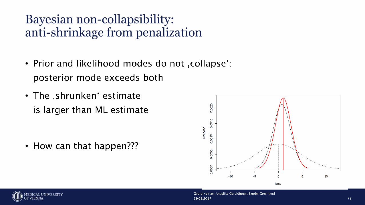
Bayesian non-collapsibility:anti-shrinkage from penalization
•
•
•

An even more extreme examplefrom Greenland 2010
•
• 𝛽1 = 0)
•
30
6
30 6 36
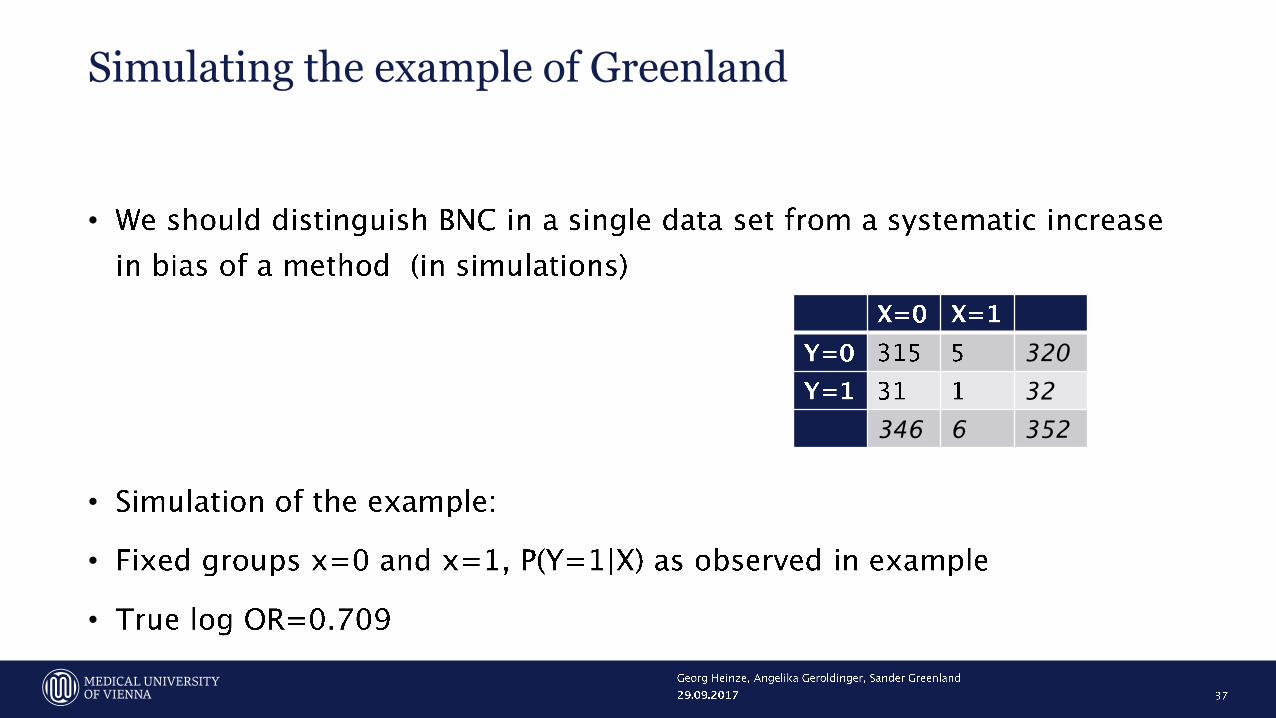
Simulating the example of Greenland
•
•
•
•
320
32
346 6 352

Simulating the example of Greenland
•
𝛽1
𝛽1
𝜷𝟏
𝛽1 −∞

Simulating the example of Greenland
•
•
•

logF(1,1) prior (Greenland and Mansournia, 2015)
•
𝐿 𝛽 ∗ = 𝐿 𝛽 ⋅ ∏𝑒
𝛽𝑗2
1+𝑒𝛽𝑗
.
∗ ∗ ∗∗ ∗ ∗∗ ∗ ∗∗ ∗ ∗∗ ∗ ∗∗ ∗ ∗∗ ∗ ∗
∗ ∗ ∗∗ ∗ ∗∗ ∗ ∗∗ ∗ ∗∗ ∗ ∗∗ ∗ ∗∗ ∗ ∗

Simulating the example of Greenland
•
𝛽1
𝛽1
𝜷𝟏
𝛽1 −∞

Simulating the example of Greenland
•
𝛽1
𝛽1
𝜷𝟏
𝛽1 −∞
Other, more subtle occurrencesof Bayesian non-collapsibility
•
•
•
•

Simulation of bivariable log reg models
• 𝑋1, 𝑋2~Bin(0.5) 𝑟 = 0.8, 𝑛 = 50
• 𝛽1 = 1.5 𝛽2 = 0.1 𝜆
𝝀
𝛽1
𝛽1
𝛽2
𝛽2
𝜷𝟐
Anti-shrinkage from penalization?
•
•
with
• ≠

Reason for anti-shrinkage
•
•
•
•
•

Example of Greenland 2010 revisited
320
32
346 6 352
321
33
347 7 352
•

FLAC: Firth‘s Logistic regression with Added Covariate
=
+
=

FLAC: Firth‘s Logistic regression with Added Covariate
𝑖=1
𝑁
𝑦𝑖 − 𝜋𝑖 𝑥𝑖𝑟 + ℎ𝑖
1
2− 𝜋𝑖 𝑥𝑖𝑟 = 0; 𝑟 = 0, … , 𝑝
ℎ𝑖 𝐻 = 𝑊1
2𝑋 𝑋′𝑊𝑋 −1𝑋𝑊1/2
𝑖=1
𝑁
𝑦𝑖 − 𝜋𝑖 𝑥𝑖𝑟 +
𝑖
𝑁
ℎ𝑖
1
2− 𝜋𝑖 𝑥𝑖𝑟 =
=
𝑖=1
𝑁
𝑦𝑖 − 𝜋𝑖 𝑥𝑖𝑟 +
𝑖=1
𝑁ℎ𝑖
2(𝑦𝑖 − 𝜋𝑖) +
𝑖=1
𝑁ℎ𝑖
2(1 − 𝑦𝑖 − 𝜋𝑖) = 0

FLAC: Firth‘s Logistic regression with Added Covariate
•
𝑖=1
𝑁
𝑦𝑖 − 𝜋𝑖 𝑥𝑖𝑟 +
𝑖=1
𝑁ℎ𝑖
2𝑦𝑖 − 𝜋𝑖 𝑥𝑖𝑟 +
𝑖=1
𝑁ℎ𝑖
21 − 𝑦𝑖 − 𝜋𝑖 𝑥𝑖𝑟 = 0
ℎ𝑖/2 ℎ𝑖/2

FLAC: Firth‘s Logistic regression with Added Covariate
•
𝑖=1
𝑁
𝑦𝑖 − 𝜋𝑖 𝑥𝑖𝑟 +
𝑖=1
𝑁ℎ𝑖
2𝑦𝑖 − 𝜋𝑖 𝑥𝑖𝑟 +
𝑖=1
𝑁ℎ𝑖
21 − 𝑦𝑖 − 𝜋𝑖 𝑥𝑖𝑟 = 0
ℎ𝑖/2 ℎ𝑖/2
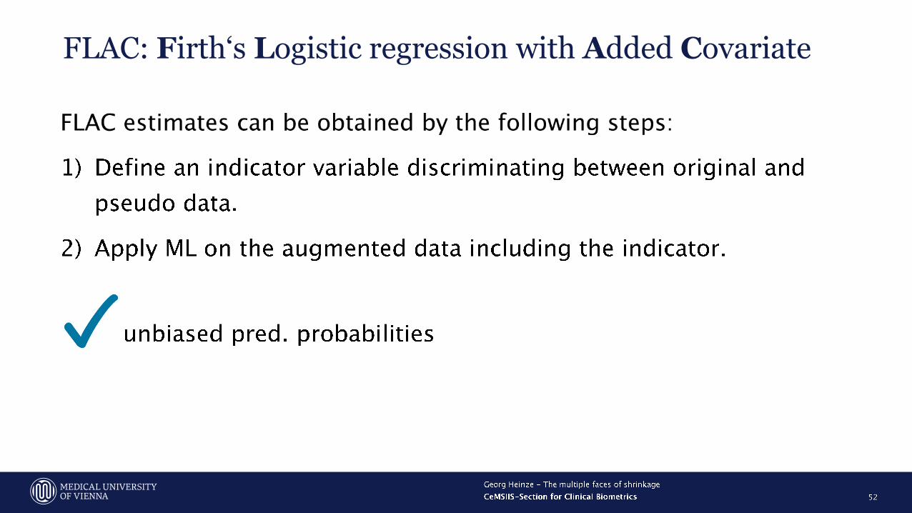
FLAC: Firth‘s Logistic regression with Added Covariate

FLIC

Simulation study: the set-up
•
•
•
•
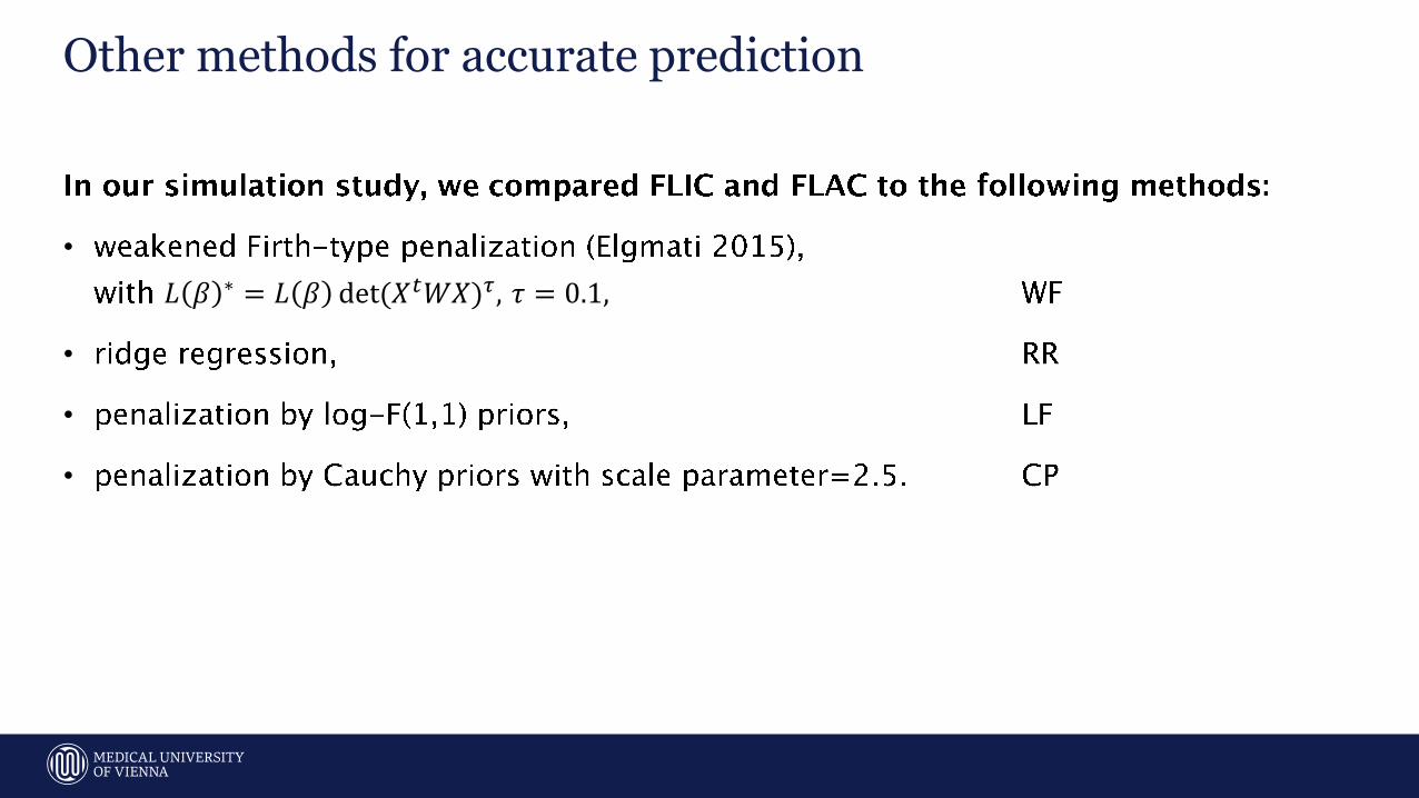
Other methods for accurate prediction
•
𝐿 𝛽 ∗ = 𝐿 𝛽 det(𝑋𝑡𝑊𝑋)𝜏, 𝜏 = 0.1,
•
•
•
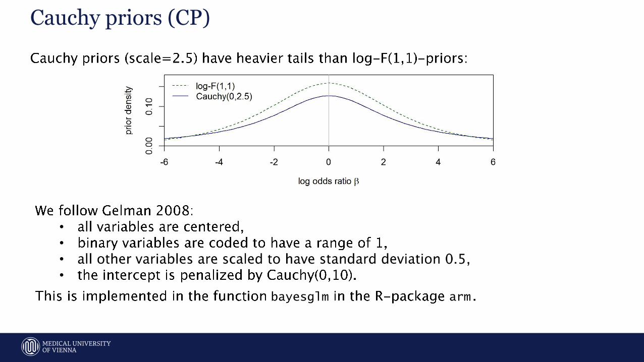
Cauchy priors (CP)
•
•
•
•
bayesglm arm.

Simulation results
• 𝛽
• 𝛽
•
• 𝜋

Predictions: bias RMSE

Predictions: bias RMSE

Predictions: bias RMSE

Predictions: bias RMSE

Predictions: bias RMSE

Predictions: bias RMSE

Predictions: bias RMSE

Predictions: bias RMSE

Comparison
FLAC
•
•
•
•
•
•
•
Bayesian methods (CP, logF)
•
• m m m
m m
• m
•
•
Ridge

Confidence intervals
•
•
• a-priori
•
• 𝛽 ± 1.96 𝑆𝐸)

Conclusion
Part 1: Prediction under model uncertainty
•
•
•
•
•
•
•
Part 2: Prediction under sparsity (fixed model)

References
•
•
•


