
Cash Flow Sensitivities With Constraints
Todd Pulvino and Vefa Tarhan*
*Northwestern University, Kellogg Graduate School of Management, and Loyola University Chicago, School of Business. We thank Matthew Billett, Tim Bollerslev, Jon Garfinkel, Michael Fishman, Charles Himmelberg, Ravi Jagannathan, Robert A. Korajczyk, Iwan Meier, Tom Nohel, Artur Raviv, Paul Spindt, Ernst Shaumburg, Steven Todd, Toni Whited, and seminar participants at DePaul University, the Federal Reserve Bank of Chicago, Financial Management Association, Loyola University Chicago, Northwestern University, Tulane University, and University of Iowa for useful discussions.

ABSTRACT Empirical studies of firms’ financing, investment, and payout policies typically examine those policies in isolation. For example, dividend policy is typically not considered when examining the determinants of capital expenditures. In this paper, we examine corporate policies simultaneously, subject to the constraint that sources of cash must equal uses of cash. We use this methodology to re-examine the investment/cashflow literature. Unlike single-equation studies that conclude that firms react to cashflow shocks by changing investments, we find that firms react by changing leverage. We conclude that failing to employ a constrained simultaneous-equation framework when examining corporate policies can cause omitted variable bias and result in large estimation errors.
1
1. Introduction
In their 1988 Brookings paper, Fazarri, Hubbard, and Petersen (hereafter FHP) document
a positive relationship between internally generated cashflow and investment. They also
find that this relationship is strongest for firms that are most likely to have difficulty
accessing external capital markets. FHP interpret their findings as evidence of a
difference between the internal and external costs of capital and conclude that capital
market frictions may cause some firms to forego positive NPV projects.
Because this result, if true, has serious implications regarding the efficiency with
which capital is allocated in the economy, it provoked a number of additional studies
examining the relationship between cashflow and investment. Many of these studies
support the original FHP findings (FHP (1996, 2000), Almeida and Campello (2002),
Boyle and Guthrie (2003), Calomiris and Hubbard (1989, 1990, and 1995), Hoshi,
Kashyap, and Scharfstein (1991), Oliner and Rudebusch (1992), Hubbard, Kashyap, and
Whited (1992), Pawlina and Renneboog (2005), Schaller (1993), Bond and Meghir
(1994), Gilchrest and Himmelberg (1995)).1, 2 Others find completely the opposite result.
For example, Kaplan and Zingales (1997 and 2000) conclude that a monotonic relation
between the degree of external market constraints and cash-flow sensitivity does not
exist.3 They find that firms with the easiest access to capital markets display the largest
1In addition to cashflow/investment sensitivity, there is evidence that constraints in accessing external capital affect other corporate decisions. For example, Korajczyk and Levy (2002) examine the connection between firms’ financial health and the timing of their financing decisions. They find that, unlike constrained firms, unconstrained firms are able to issue securities at economically favorable times. 2 Minton and Schrand (1999) find that higher cashflow volatility increases the cost of external capital, and hence results in higher investment cashflow sensitivity. In particular they find that higher volatility is correlated with lower capital expenditures, R&D, and advertising expenses. 3 Others such as Moyen (2004),and Alti (2003) find support for both camps. For example, Moyen, using generated data, finds that the results obtained from her unconstrained model support Kaplan and Zingales. However, she also finds that cashflow sensitivity is higher for low dividend paying firms than it is for high dividend paying firms, supporting the results of FHP.

2
sensitivity of investment to cash flow. Firms that are financially constrained have the
next largest sensitivity, and firms that are partially constrained are least sensitive. Their
findings imply that investment/cashflow sensitivities are uncorrelated with access to
capital markets. Using a larger sample of firms, Cleary (1999) confirms Kaplan and
Zingales’ conclusion. In fact, Cleary finds that investment-cash flow sensitivities are
actually inversely related to constraints--the most constrained firms have the lowest
sensitivities and the least constrained firms have the highest sensitivities.
Econometric problems associated with model misspecification may be the cause
of the lack of consensus in the literature. The existing literature examines the cash flow
sensitivity of investment in isolation, that is, without accounting for the simultaneous
effect that cash flows have on investment and financing decisions. When investment and
financing decisions are condensed into a single capital expenditure equation, the
estimated cashflow sensitivity coefficient is likely to suffer from omitted variable bias.
Single-equation models are also likely to produce inefficient coefficient estimates
because they do not exploit the information contained in the constraint that sources and
uses of cash must be equal. In addition to econometric problems, single-equation models
produce coefficient estimates that are difficult to interpret from an economic perspective.
For example, observing that capital expenditures and cashflows are uncorrelated is
consistent with the absence of financing constraints. However, it is also consistent with
the existence of financing constraints if firms insulate capital expenditures by increasing
asset sales to compensate for cashflow shortfalls.
In this paper, we propose a model in which firms make their investment and
financing decisions jointly, subject to the constraint that sources and uses of funds are

3
equal. The model follows James Tobin’s suggestion, in his discussion of the original
FHP article, that “… the firm jointly determines investment, dividend payments, and
other ways of allocating its cash flow. Therefore,…the authors (should) model
investment and dividends as depending on the same set of explanatory variables.” Put
differently, a firm’s investment, financing, and distribution decisions are necessarily
interrelated by the identity that sources of funds equal uses of funds.4 A firm that
experiences a one dollar increase in operating cash flow could increase capital
expenditures, say, by one dollar.5 However, it could also use the incremental cash flow
to pay down debt, increase shareholder distributions, or make any combination of
investment and financing decisions that result in a net response of one dollar. Ex-post,
this constraint holds precisely. Ex-ante, it holds in expectation.
Specifically, our model contains nine equations describing the investment (capital
expenditures, acquisitions, and asset sales), financing (short-term debt issues, long-term
debt issues, and changes in cash balances), and distribution (equity issues, dividends, and
share repurchases) decisions that firms make. We estimate this model using a sample
that covers 1950-2003.
Our simultaneous equation model extends the literature in two primary ways.
First, it provides an empirical estimate of the size of the omitted variable bias that results
from estimating the capital expenditure/cashflow sensitivity in isolation. Second, rather
4 While there are no papers that estimate a system of cashflow sensitivity equations subject to the sources and uses of funds constraint, there are some papers that examine cashflow sensitivity of selected sources/uses variables. For example Gilchrist and Himmelberg (1998) use a structural model to find the marginal cost of funds and examine how it relates to debt, cash, and working capital. Also Fazzari and Petersen (1993), examine the cashflow sensitivity of working capital. Additionally, Almeida, Campello, and Weisbach (2002), develop a model of how cash holdings respond to cashflow changes (cashflow sensitivity of cash). Our results do not support their prediction that more of the cashflow increases will be used to build up the cash holdings in the case of the constrained firms compared with unconstrained firms.

4
than focusing solely on capital expenditures, it provides a description of how firms adjust
leverage, distributions, and other investment decisions in response to a change in
cashflow. By examining each of these responses simultaneously, we are able to make
more accurate inferences regarding effects of potential capital constraints on investment.
For example, we are able to determine whether firms respond to negative changes in
cashflow by cutting investment and maintaining leverage (consistent with an inability to
access external capital) or by maintaining investment and increasing leverage (consistent
with an absence of capital constraints).
Our empirical analyses yield three primary findings. First, contrary to previously
published studies, the cash flow sensitivity of investments is small, regardless of the
firm’s financial health. Estimating our multi-equation model using the full sample, a one
dollar increase in cash flow produces a statistically insignificant $0.001 increase in
capital expenditures. In contrast, previously published single-equation studies typically
find that a one dollar increase in cash flow results in an increase in capital expenditures
ranging between $0.10 and $0.25, a result that we are able to replicate using a single-
equation analysis.
Second, we find that a firm’s primary response to a change in cashflow is to
adjust financial leverage. Unlike investment/cashflow sensitivities, financing/cashflow
sensitivities are large and highly significant, regardless of the firm’s financial health.
Using the full sample, a one dollar increase in cashflow results in a $0.78 decrease in
total debt and a $0.23 increase in cash balance. Thus, our results show that net debt
changes by approximately one dollar in reaction to a one dollar change in cashflow. This
5 In fact, the firm in question could even increase its capital expenditures even by more than a dollar, if the increase in the cashflow increases the firms’ debt and/or external equity capacity by more than a dollar.

5
result implies the absence of a systematic underinvestment problem. If such a problem
existed, we would observe firms spending a portion of the incremental cashflow to
undertake new projects, rather than retiring capital. It is not possible to obtain this
evidence from single-equation investment models that examine the capital
expenditure/cashflow sensitivity in isolation.
Third, when we partition the sample on the basis of positive and negative
cashflow changes, we observe that both the investment and financing sensitivities are
symmetric.6 For the full sample, a one dollar cashflow decrease causes firms to borrow
an additional $0.80 whereas a one dollar cashflow increase causes firms to repay $0.76 of
debt. What is more remarkable is that the symmetry holds even for the subsample of
firms that are classified as being “financially constrained”. Firms in the financially
constrained subsample borrow $0.81 in response to a $1 reduction in cashflow and reduce
debt by $0.75 when they experience a positive one dollar change in cashflow. The
borrowing ability of firms that are perceived to have the weakest financial health, in an
environment when they are experiencing negative cashflow shocks, combined with the
small investment/cashflow sensitivity, provides strong evidence that impediments to
accessing capital markets have little impact on firms’ investment decisions.
The organization of the rest of the paper is as follows. Section 2 contrasts our
system of equations model with the single-equation models employed in the literature. In
Section 3, we develop the simultaneous-equations model that we use in our estimations.
The data are described in Section 4. Section 5 presents and discusses empirical results
and section 6 concludes.
6We thank the associate editor for suggesting that we estimate our model for both positive and negative cashflow changes.
6
2. Single Equation versus System of Equation Models
Single-equation models used to study the effect of capital constraints on
investment typically estimate the following equation:
ttt
t
t
t MBK
CFK
CAPXεββ ++= 21
(1)
where CAPX is capital expenditures, K is fixed assets, CF is cashflow, and MB is the
ratio of the market value of assets to the book value of assets. A common interpretation
of the cashflow coefficient in equation (1) is that a relatively small coefficient implies
that firms can immunize capital expenditures against adverse cashflow realizations.
Conversely, a relatively large positive coefficient is often interpreted as evidence that
firms respond to negative cashflow realizations by decreasing capital expenditures, a
reaction that is consistent with costly access to external capital. To determine whether
capital constraints affect investment, equation (1) is typically estimated using samples of
firms with different states of financial health. The underlying hypothesis is that
financially unhealthy firms are more likely to face capital constraints, and should
therefore have a larger investment/casfhlow coefficient than financially healthy firms.
Prior studies that estimate equation (1) consistently find a positive relationship
between capital expenditures and cashflow. As shown in Table 1, coefficient estimates
between 0.10 and 0.25 are common. Using our sample of firms to estimate equation (1),
and after matching the sample period and selection criterion in Cleary (1999), produces a
coefficient estimate of 0.16.7 Based on the interpretation that is common in the literature,
7 For Table 1 only, we restrict the sample to 1987-1994 to match the period used by Cleary (1999).
7
this implies that a one dollar decrease in cashflow results in a $0.16 decrease in capital
expenditures.
The problem with this interpretation is that it requires an implicit assumption that
firms do not systematically adjust to cashflow revelations by altering other sources and
uses of cash. Instead, alternate responses such as raising debt or equity, or selling assets,
are subsumed in the error term. This can be problematic if the omitted variables are
correlated with cash flows, in which case the cashflow coefficient may be biased. For
example, the direct effect of a negative cashflow shock may be a reduction in capital
expenditures. However, an indirect effect may be an increase in debt financing and a
commensurate increase in capital expenditures. To determine the total effect on capital
expenditures of a negative cashflow shock, both the direct and indirect effects must be
considered simultaneously.
In addition to inducing a bias, failing to simultaneously account for the direct and
indirect effects can lead to incorrect conclusions regarding firms’ abilities to finance their
projects by raising external capital. For example, consider two firms, one of which is
financially unconstrained and the other financially constrained. Each firm faces a one
dollar decrease to cashflow. The unconstrained firm reacts by cutting capital
expenditures by $0.20 and by issuing debt worth $0.80. The constrained firm is unable to
access external capital and instead responds by cutting capital expenditures by $0.20 and
by selling $0.80 worth of assets. In this example, a single-equation model would show
identical investment/cashflow sensitivities even though one firm is unconstrained and the
other is constrained. The presence of financial constraints is evident not in the
investment/cashflow sensitivity, but in the debt/cashflow sensitivity.
8
A second example shows that interpreting a positive investment/cashflow
sensitivity relation as evidence of financial constraints can also be problematic. Consider
a firm that responds to a one dollar decrease in cashflow by altering its strategy from one
of organic growth to one of debt-financed acquisitions. Because organic growth is
reduced, capital expenditures will decrease leading to a positive investment/cashflow
sensitivity. However, in this example, the firm is not financially constrained as it was
able to access the debt markets to obtain financing for acquisitions.
It is possible to construct other examples that suggest that inferences regarding
access to capital markets cannot be made solely on the basis of investment/cashflow
sensitivities as is typical in single-equation studies. However, it is difficult to
systematically quantify the sign and magnitude of the resulting bias induced by ignoring
the firm’s other decision variables, especially when the full array of decision variables
available to the firm are considered. Therefore, rather than attempting to quantify the
bias analytically, we measure the bias empirically by estimating the simultaneous-
equation model described in the following section.
3. Model
The manager’s task is to select optimal values for investment and financing
decision variables, given the expected values for exogenous and predetermined variables.
Table 2 describes the variables that enter the optimization problem. In solving this
problem, the manager faces the constraint that ex-post, sources of funds must equal uses
of funds:
ttttttttttt OTHERCFASALESEQUISSSTDLTDACQUISCAPXDIVRPCash +≡−−Δ−Δ−++++Δ (2)
9
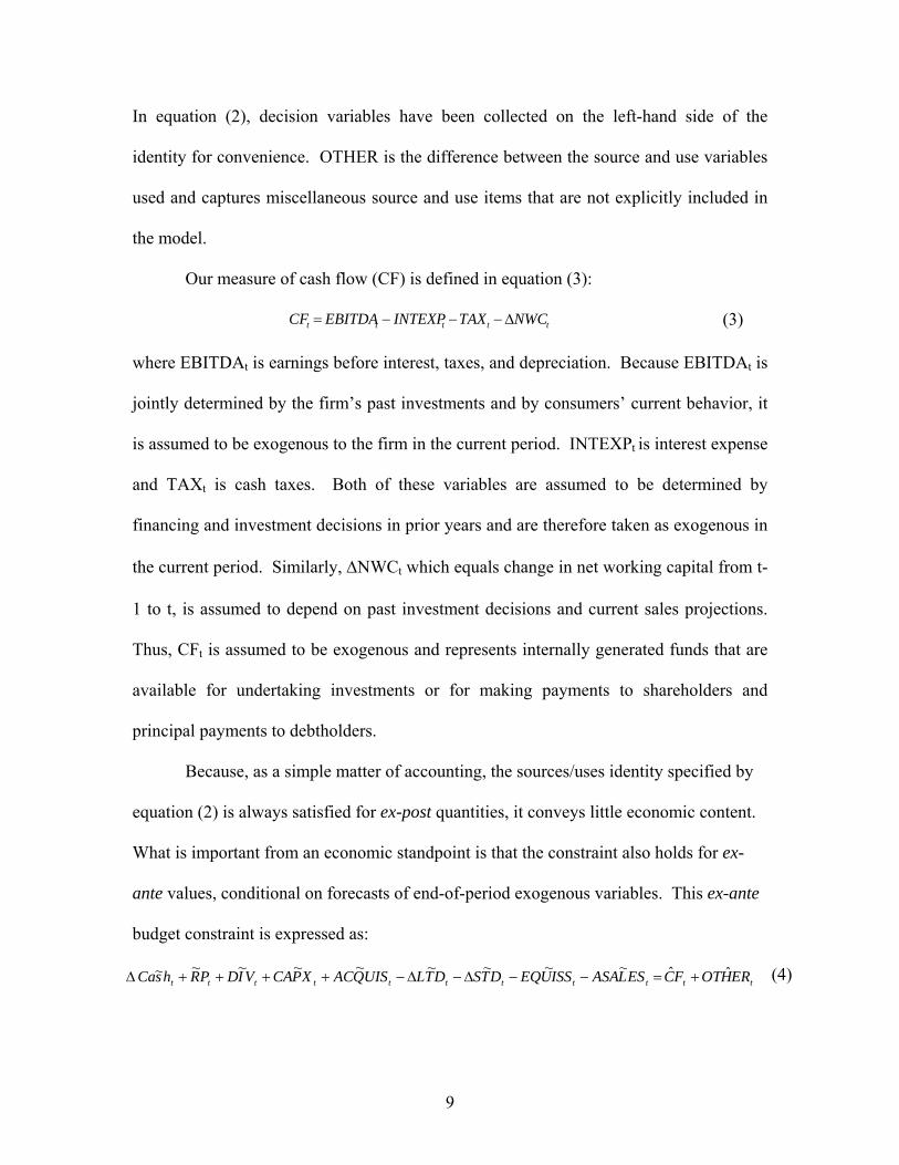
In equation (2), decision variables have been collected on the left-hand side of the
identity for convenience. OTHER is the difference between the source and use variables
used and captures miscellaneous source and use items that are not explicitly included in
the model.
Our measure of cash flow (CF) is defined in equation (3):
ttttt NWCTAXINTEXPEBITDACF Δ−−−= (3)
where EBITDAt is earnings before interest, taxes, and depreciation. Because EBITDAt is
jointly determined by the firm’s past investments and by consumers’ current behavior, it
is assumed to be exogenous to the firm in the current period. INTEXPt is interest expense
and TAXt is cash taxes. Both of these variables are assumed to be determined by
financing and investment decisions in prior years and are therefore taken as exogenous in
the current period. Similarly, ΔNWCt which equals change in net working capital from t-
1 to t, is assumed to depend on past investment decisions and current sales projections.
Thus, CFt is assumed to be exogenous and represents internally generated funds that are
available for undertaking investments or for making payments to shareholders and
principal payments to debtholders.
Because, as a simple matter of accounting, the sources/uses identity specified by
equation (2) is always satisfied for ex-post quantities, it conveys little economic content.
What is important from an economic standpoint is that the constraint also holds for ex-
ante values, conditional on forecasts of end-of-period exogenous variables. This ex-ante
budget constraint is expressed as:
ttttttttttt ERHOTFCESLASAISSUEQDTSDTLUISQACXPCAVIDPRhsCa ˆˆ~~~~~~~~~ +=−−Δ−Δ−++++Δ (4)

10
where tildes represent decision variables and hats represent exogenous variables that
must be forecasted. Equation (4) states that at the beginning of period t, when firms
make their investment and financing decisions, the planned values of decision variables
are selected such that the expected end-of-period sources/uses constraint is satisfied.
This implies that a firm cannot plan to allocate funds in excess or deficit of the amount it
expects to generate, either through operations or financing, during the current period.
For choice variables, ex-ante quantities are planned values, determined based on
beginning-of-period known quantities. While the firm has precise control over ex-ante
(planned) levels, ex-post quantities depart stochastically from their ex-ante counterparts
as follows:
⎥⎥⎥⎥⎥⎥
⎦
⎤
⎢⎢⎢⎢⎢⎢
⎣
⎡
+
⎥⎥⎥⎥⎥⎥
⎦
⎤
⎢⎢⎢⎢⎢⎢
⎣
⎡
Δ−
Δ
−−
=
⎥⎥⎥⎥⎥⎥
⎦
⎤
⎢⎢⎢⎢⎢⎢
⎣
⎡
Δ−Δ
−−
Δ
Δ
tCASH
tLTD
tACQUIS
tCAPX
t
t
t
t
t
t
t
t
ee
ee
SHAC
DTL
UISQACXPCA
CASHLTD
ACQUISCAPX
,
,
,
,
~
~
~~
MMM
(5)
eCAPX,t,.... eCASH,t are error terms associated with the nine financing and investment
decision variables, and represent deviations of actual quantities from planned quantities.
Similarly, ex-post exogenous source variables (CF and OTHER) equal forecasts of these
variables made at the beginning of the period plus forecast errors:
⎥⎦
⎤⎢⎣
⎡+⎥
⎦
⎤⎢⎣
⎡=⎥
⎦
⎤⎢⎣
⎡
tOTHER
tCF
tt
t
ee
ERHOTFtC
OTHERCF
,
,
ˆˆ
(6)
Taken together, equations (4), (5), and (6) imply that the error terms are related in the
following manner:
11
tttttttttt OTHERCFASALESEQUISSSTDLTDtACQUISCAPXDIVRPCash eeeeeeeeeee +=−−−−++++ ΔΔΔ (7)
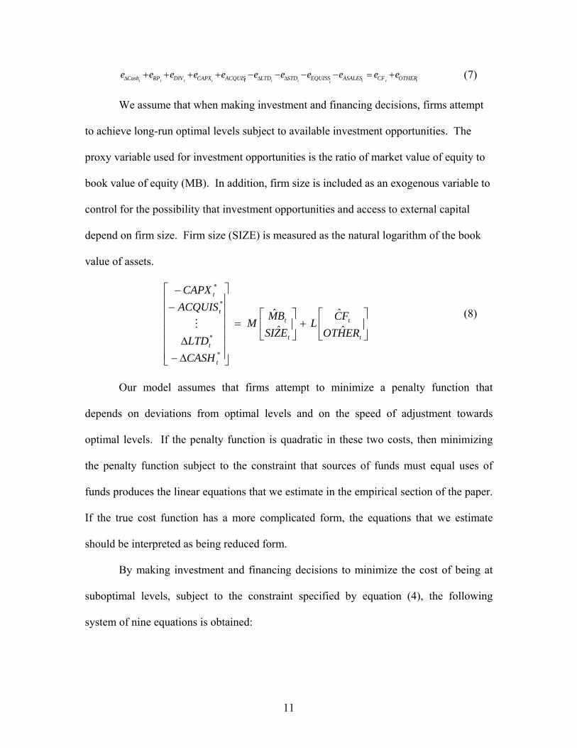
We assume that when making investment and financing decisions, firms attempt
to achieve long-run optimal levels subject to available investment opportunities. The
proxy variable used for investment opportunities is the ratio of market value of equity to
book value of equity (MB). In addition, firm size is included as an exogenous variable to
control for the possibility that investment opportunities and access to external capital
depend on firm size. Firm size (SIZE) is measured as the natural logarithm of the book
value of assets.
⎥⎦
⎤⎢⎣
⎡+⎥
⎦
⎤⎢⎣
⎡=
⎥⎥⎥⎥⎥⎥
⎦
⎤
⎢⎢⎢⎢⎢⎢
⎣
⎡
Δ−Δ
−−
t
t
t
t
t
t
t
t
ERHOTFCL
EZSIBMM
CASHLTD
ACQUISCAPX
ˆˆ
ˆˆ
*
*
*
*
M
(8)
Our model assumes that firms attempt to minimize a penalty function that
depends on deviations from optimal levels and on the speed of adjustment towards
optimal levels. If the penalty function is quadratic in these two costs, then minimizing
the penalty function subject to the constraint that sources of funds must equal uses of
funds produces the linear equations that we estimate in the empirical section of the paper.
If the true cost function has a more complicated form, the equations that we estimate
should be interpreted as being reduced form.
By making investment and financing decisions to minimize the cost of being at
suboptimal levels, subject to the constraint specified by equation (4), the following
system of nine equations is obtained:
12
⎥⎦
⎤⎢⎣
⎡+⎥
⎦
⎤⎢⎣
⎡+
⎥⎥⎥⎥⎥⎥
⎦
⎤
⎢⎢⎢⎢⎢⎢
⎣
⎡
Δ−Δ
−−
=
⎥⎥⎥⎥⎥⎥
⎦
⎤
⎢⎢⎢⎢⎢⎢
⎣
⎡
Δ−Δ
−−
−
−
−
−
t
t
t
t
t
t
t
t
t
t
t
t
ERHOTFCL
EZSIBMM
CASHLTD
ACQUISCAPX
K
SHACDTL
UISQACPXAC
ˆˆ
ˆˆ
~~
~~
1
1
1
1
MM
(9)
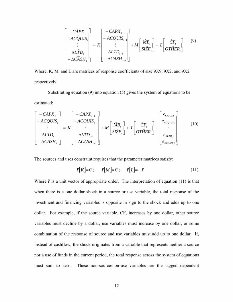
Where, K, M, and L are matrices of response coefficients of size 9X9, 9X2, and 9X2
respectively.
Substituting equation (9) into equation (5) gives the system of equations to be
estimated:
⎥⎥⎥⎥⎥⎥
⎦
⎤
⎢⎢⎢⎢⎢⎢
⎣
⎡
+⎥⎦
⎤⎢⎣
⎡+⎥
⎦
⎤⎢⎣
⎡+
⎥⎥⎥⎥⎥⎥
⎦
⎤
⎢⎢⎢⎢⎢⎢
⎣
⎡
Δ−Δ
−−
=
⎥⎥⎥⎥⎥⎥
⎦
⎤
⎢⎢⎢⎢⎢⎢
⎣
⎡
Δ−Δ
−−
Δ
Δ
−
−
−
−
tCASH
tLTD
tACQUIS
tCAPX
t
t
t
t
t
t
t
t
t
t
t
t
ee
ee
ERHOTFCL
EZSIBMM
CASHLTD
ACQUISCAPX
K
CASHLTD
ACQUISCAPX
,
,
,
,
1
1
1
1
ˆˆ
ˆˆ
MMM
(10)
The sources and uses constraint requires that the parameter matrices satisfy:
[ ] [ ] [ ] '';'0';'0' iLiMiKi −=== (11)
Where i' is a unit vector of appropriate order. The interpretation of equation (11) is that
when there is a one dollar shock in a source or use variable, the total response of the
investment and financing variables is opposite in sign to the shock and adds up to one
dollar. For example, if the source variable, CF, increases by one dollar, other source
variables must decline by a dollar, use variables must increase by one dollar, or some
combination of the response of source and use variables must add up to one dollar. If,
instead of cashflow, the shock originates from a variable that represents neither a source
nor a use of funds in the current period, the total response across the system of equations
must sum to zero. These non-source/non-use variables are the lagged dependent
13
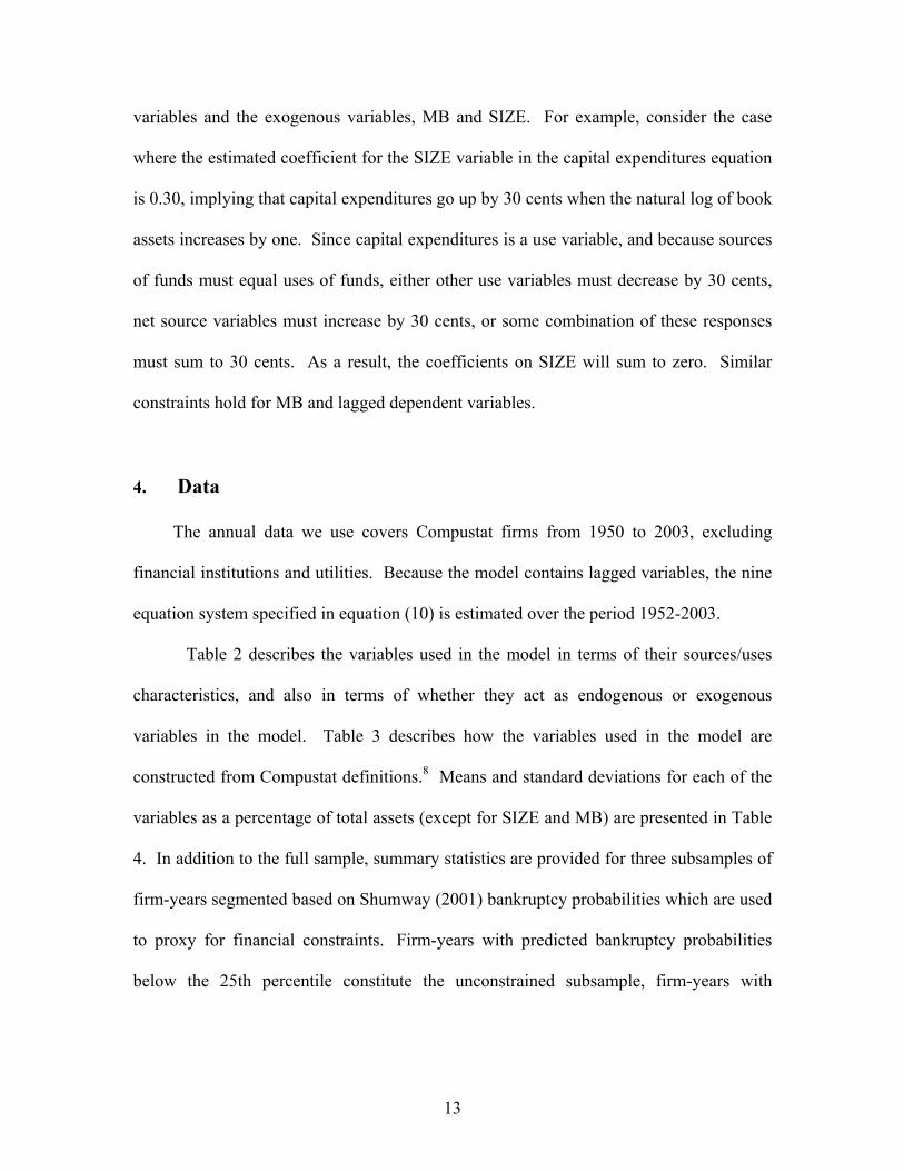
variables and the exogenous variables, MB and SIZE. For example, consider the case
where the estimated coefficient for the SIZE variable in the capital expenditures equation
is 0.30, implying that capital expenditures go up by 30 cents when the natural log of book
assets increases by one. Since capital expenditures is a use variable, and because sources
of funds must equal uses of funds, either other use variables must decrease by 30 cents,
net source variables must increase by 30 cents, or some combination of these responses
must sum to 30 cents. As a result, the coefficients on SIZE will sum to zero. Similar
constraints hold for MB and lagged dependent variables.
4. Data
The annual data we use covers Compustat firms from 1950 to 2003, excluding
financial institutions and utilities. Because the model contains lagged variables, the nine
equation system specified in equation (10) is estimated over the period 1952-2003.
Table 2 describes the variables used in the model in terms of their sources/uses
characteristics, and also in terms of whether they act as endogenous or exogenous
variables in the model. Table 3 describes how the variables used in the model are
constructed from Compustat definitions.8 Means and standard deviations for each of the
variables as a percentage of total assets (except for SIZE and MB) are presented in Table
4. In addition to the full sample, summary statistics are provided for three subsamples of
firm-years segmented based on Shumway (2001) bankruptcy probabilities which are used
to proxy for financial constraints. Firm-years with predicted bankruptcy probabilities
below the 25th percentile constitute the unconstrained subsample, firm-years with

14
predicted bankruptcy probabilities above the 75th percentile constitute the constrained
subsample, and firm-years that fall between the above two percentiles constitute the
partially constrained subsample. Splitting the sample in this way results in an uneven
number of firms in each subsample—the partially constrained subsample contains
approximately two times the number of firm-years as do the constrained and
unconstrained subsamples. The benefit of this method of segmentation over a simple
trifurcation of the sample is that the identification of constrained and unconstrained firm-
years is more accurate.
Table 4 shows that mean cashflow (as a percent of total assets) increases
monotonically with financial health. The mean cashflow for the financially
unconstrained subsample is twice as large as the mean cashflow for the partially
constrained subsample. Furthermore, mean cashflow is negative for the financially
constrained subsample. There is a similarly monotonic relationship between dividends
and financial health. Unconstrained firms pay larger dividends (as a percent of total
assets) than constrained firms. Additionally, reliance on short-term debt increases
monotonically, as financial health deteriorates.
Market-to-book ratio is used in the regressions as a proxy for investment
opportunities. Based on this proxy, unconstrained firms have the richest investment
opportunities, while financially constrained firms have the poorest investment
opportunities. Financially unconstrained firms, which have high market-to-book ratios
also appear to be less acquisitive, which is consistent with these firms having healthy
internal growth opportunities. Finally, like the market-to-book ratio, firm size exhibits a
8 To avoid dropping observations with missing Compustat variables, we replace missing data with zero. We also estimated the model after dropping observations with missing data. Results are not significantly

15
monotonic relationship with financial health—unconstrained firms tend to be larger
whereas financially constrained firms tend to be smaller.
5. Empirical Results
The system specified in equation (10) is estimated using two methods for forecasting
the endogenous variables. The first forecast model, which we refer to as the perfect
foresight model, assumes that planned values of the decision variables equal end-of-
period (ex-post) realizations of these variables. The second forecast model uses I/B/E/S
analysts' forecasts to construct estimates of internally generated cash flow (CF).9
Because both approaches generate similar estimates, results only from the perfect
foresight model are reported. The model is first estimated for the full sample using levels
(not first differences) without firm and year fixed effects. Following this, results are
presented using first differences for subsamples of data based on firms’ financial health.
5.1 . Model Estimation
Results from estimating equation (10) subject to the restriction specified by equation
(11) are shown in Tables 5A and 5B. The estimation uses the full sample, consisting of
affected by how missing data is treated. 9 Forecasted cashflow is measured using the following equation:
[ ] XIDONICSHOIBFIMDCFFC −−+= ))((~
where IBFIMD is the median earnings per share estimate for the current fiscal year provided by I/B/E/S, CSHO is common shares outstanding, NI is net income, and XIDO is extraordinary items and discontinued operations (all Compustat annual mnemonics.) The first term in the above equation is the realized cashflow. The second term adjusts realized cashflow to reflect differences between expected and actual net income. Finally, extraordinary items are subtracted to reflect the fact that had they been expected, they would be unlikely to be extraordinary.

16
244,081 firm-years. The regressions are estimated with robust standard errors that
account for within-firm clustering (18,849 clusters.)
Estimated responses of each of the endogenous financing and investment variables to
changes in cash flow, the residual sources/uses variable (OTHER), market-to-book ratio,
and firm size are reported in Table 5A. Column 1 displays the casfhlow coefficients. As
expected, a one dollar increase in casfhlow results in an increase in “use” variables and a
decrease in “source” variables. In the case of use variables, the coefficients in the first
column of Table 5A show that a one dollar increase in cashflow causes a $0.03 increase
in capital expenditures (statistically insignificant), a $0.01 increase each in dividends and
share repurchases, and a $0.24 increase in cash balances (all statistically significant).
The first column of Table 5A also shows that positive cashflow innovations cause
other source variables to decline. Firms react to a $1 cashflow shock by retiring $0.15 of
long-term, and $0.58 of short-term debt. Both of the estimated debt coefficients are
statistically different from zero at the 1% level. Asset sales and equity issues remain
unchanged while acquisitions decline (significant at the 10 percent level.) In all, 7 of the
8 coefficients in the estimated system have the expected sign, and the shareholder
distribution and leverage variables are significant at the 1% level.
Because of the constraint specified in equation (11), a one dollar increase in
cashflow must result in a one dollar decrease in other sources of funds, a one dollar
increase in uses of funds, or some combination of a reduction in sources or increase in
uses to exactly offset the one dollar cashflow increase. The coefficients reported in the
first column of Table 5A show that this indeed is the case—use variables increase by
$0.27, while source variables decrease by $0.73. While the sign of both total uses and

17
total sources are as expected, the primary conclusion that emerges from these results is
that financing/cashflow sensitivities dominate investment/cashflow sensitivities. Net
debt (long-term debt plus short-term debt minus cash balance) decreases by $0.97 and net
investments increase by a meager $0.02 (capital expenditures increase by $0.03.)
The variable OTHER in Table 5A is defined to be the difference between
miscellaneous source and use variables not explicitly accounted for in the model. For
example, a decrease in “other assets” represents a source of funds as does an increase in
“other liabilities.” Neither one of these balance sheet accounts is explicitly modeled
since they do not represent economically important decisions. Thus, the effects of all
miscellaneous sources and uses are subsumed in OTHER. Because of the way in which
OTHER is defined, it has an interpretation that is similar to the cash flow variable. A one
dollar shock in OTHER must be offset by a one dollar increase in uses, a one dollar
decrease in other sources, or some combination of the two. As is the case for cashflow
shocks, results displayed in the second column of Table 5A show that long-term and
short-term debt are the primary buffers to changes in other assets and liabilities.
The final variables in Table 5A are market-to-book ratio (MB) and firm size
(SIZE). Since these variables represent neither sources nor uses of funds, the response of
the system to innovations in these variables sums to zero. Results shown in the fourth
column of Table 5A suggest that firms with higher market-to-book ratios are more likely
to issue equity. When distributing cash to shareholders, high market-to-book ratio firms
rely more on share repurchases and less on dividends. High market-to-book ratio firms
are also likely to reduce both short and long-term debt compared to low market-to-book
ratio firms. Overall, these results are consistent with what one would expect of firms

18
with significant growth opportunities. Size is also related to firms’ investment, financing,
and distribution decisions. In general, larger firms appear to be more active participants
in financial markets, having higher levels of acquisitions, equity issues, dividend
payments, share repurchases, and both long and short-term debt issues.
Coefficients for the lagged endogenous variables (estimates for matrix K in
equation (10)) are displayed in Table 5B. The estimated coefficients of the matrix
describe how current investment and financing variables depend on lagged investment
and financing variables. Diagonal elements of K can be loosely interpreted as “own”
adjustment rates; the smaller in absolute value is the jth diagonal coefficient, the less
inertia is displayed in the adjustment of the jth variable. Dividends, capital expenditures,
and asset sales display the most inertia, with lagged coefficients of 0.92, 0.87, and 0.84,
respectively. These coefficients reflect the sticky nature of dividends, and the multi-year
nature of capital expenditure programs. Conversely, leverage variables (long and short-
term debt issues, and change in cash balances) show very little inertia, indicating that
these variables adjust quickly to shocks. In addition, debt variables respond strongly in
the current period to lagged capital expenditures (both in terms of magnitude and
statistical significance) reflecting the use of debt to finance capital expenditure programs.
Off-diagonal elements provide evidence that changes in cash balances and both
long and short-term debt issues act as “shock absorbers” in the system. In general, the
largest off–diagonal elements (in absolute value) are found in the rows associated with
these three leverage variables, implying that current-period cash holdings and debt issues
respond strongly to prior changes in other system variables. Conversely, columns
associated with leverage variables have by far the smallest off-diagonal coefficients

19
indicating that lagged changes in these variables do not influence the rest of the system in
the current period. In sum, the relative sizes (in absolute value) of the off-diagonal rows
and columns, along with small diagonal coefficients, suggest that debt absorbs, but does
not transmit, shocks to the rest of the system.
5.2. Model Estimation Using First Differences
Because of the cross-sectional nature of the analysis described in the preceding
section, regression coefficients reflect differences in capital expenditures across firms
rather than within firms. Therefore, they provide only an indirect estimation of how
individual firms alter investment and financing variables in response to cashflow shocks.
To provide a more direct estimate, we first transform all variables from levels to first
differences and use time dummies to account for fixed firm and year effects. The model
in first differences must satisfy the constraint that changes in sources of funds equal
changes in uses of funds.10
Results from estimating the first-difference version of the model are presented in
Table 6. For brevity, only cashflow coefficients and adjusted R2 for each of the nine
equations are presented. To facilitate comparison, cashflow coefficients reported in
Table 5A using levels rather than first differences are replicated in Table 6. Table 6
shows that using first differences provides even stronger evidence that firms respond to
cashflow shocks by altering financing rather than investment variables. The cashflow
coefficient from the capital expenditures equation is 0.001 using first differences versus
10 Cleary (1999) does not use first differences, but instead transforms variables by subtracting firm and year means. In our analysis, transforming variables in this way makes it difficult to interpret the sources/uses constraint. Nevertheless, we also performed the analysis using this transformation. Results (unreported) are nearly identical to those obtained using first differences.

20
0.031 using levels. This implies that a one dollar cashflow change affects capital
expenditures by less than one penny. The first difference analysis confirms that firms
react to cashflow changes primarily by altering debt and cash balances. A one dollar
decrease in cashflow causes long-term debt to increase by $0.14, short-term debt to
increase by $0.63, and cash balances to decrease by $0.23. In addition, there is an
economically small but statistically significant decrease in share repurchases. Overall,
results presented in Table 6 indicate that firms do not cut capital expenditures in response
to negative cashflow shocks but instead react by increasing net debt.
5.3. Effects of Capital Constraints
Prior investment/cashflow studies focus on whether constraints in accessing
external capital affect firms’ investment levels. Based on results presented in Tables 5
and 6, there is little evidence that financing constraints alter investment levels for the
broad sample. However, the effect could be absent for the majority of firms, but might
still exist for financially unhealthy firms. The approach taken in prior studies is to
segment the sample based on some measure of financial health and then determine
whether there is a relationship between financial health and investment/cashflow
sensitivity. In their original paper, FHP (1988) segmented firms according to dividend
payout ratios. Firms that paid no dividends were deemed to be financially constrained,
firms that paid small dividends relative to net income were deemed to be partially
financially constrained, and firms that paid moderate-to-large dividends relative to net
income were deemed to be unconstrained. Subsequent papers questioned the legitimacy
of simply using dividend levels as a determinant of financial health and instead used a

21
range of financial variables to classify firms’ financial health. For example, Cleary
(1999) uses multiple discriminant analysis, similar to that used by Altman to generate Z
scores for bankruptcy prediction. To conduct the discriminant analysis, Cleary generates
three groups of firms. Firms that decrease their dividends in a given period are placed in
Group 1, firms that increase their dividend are placed in Group 2, and firms that leave
their dividends unchanged are placed in Group 3. Using financial variables that are likely
to reflect a firms’ classification into Group 1 or Group 2, Cleary calculates ZFC, a pseudo
Z-Score that reflects a firm’s degree of financial constraint. In this paper, we follow a
similar approach. However, because firms alter dividend policies for many reasons
unrelated to financial constraints, we segment firms by bankruptcy probability rather than
change in dividend policy.11
There are a number of ways to calculate bankruptcy probability. Perhaps the best
approach would be to use a Merton-type model that accounts for the volatility of the
firm’s assets as well as the firm’s capital structure (Merton 1974.) Yet because of
problems in estimating asset volatility and in gathering detailed capital structure data for
individual firms, this approach is cumbersome to implement over a large sample. An
alternative approach is to use bankruptcy probabilities calculated using reduced-form
models such as the Altman Z-Score model or the Shumway (2001) hazard model. Both
of these models are easy to implement and provide reasonably accurate rankings of
financial health. Shumway’s hazard model in particular has been shown to produce
results that are similar to those produced using the Merton asset-based model (Bharath
11 In addition to segmenting the data using the Shumway (2001) bankruptcy probability model, we also formed subsamples by using Altman’s Z-Scores, and by replicating Cleary’s (1999) discriminant analysis with bootstrapped standard errors (table available upon request.) All three approaches produce similar results indicating that the analysis is robust to subsample formation and standard error estimation.
22
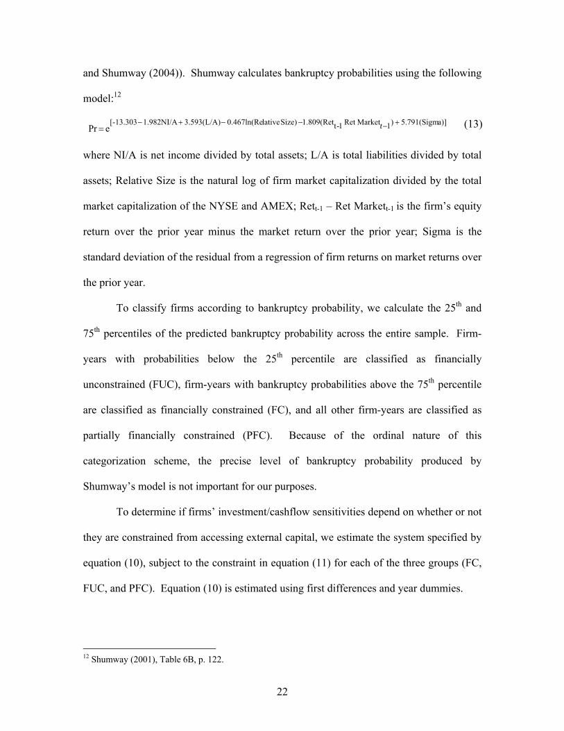
and Shumway (2004)). Shumway calculates bankruptcy probabilities using the following
model:12
a)]5.791(Sigm)1MarketRet1-t1.809(RetSize)lative0.467ln(Re3.593(L/A)1.982NI/A[-13.303ePr
+−−−+−= t (13)
where NI/A is net income divided by total assets; L/A is total liabilities divided by total
assets; Relative Size is the natural log of firm market capitalization divided by the total
market capitalization of the NYSE and AMEX; Rett-1 – Ret Markett-1 is the firm’s equity
return over the prior year minus the market return over the prior year; Sigma is the
standard deviation of the residual from a regression of firm returns on market returns over
the prior year.
To classify firms according to bankruptcy probability, we calculate the 25th and
75th percentiles of the predicted bankruptcy probability across the entire sample. Firm-
years with probabilities below the 25th percentile are classified as financially
unconstrained (FUC), firm-years with bankruptcy probabilities above the 75th percentile
are classified as financially constrained (FC), and all other firm-years are classified as
partially financially constrained (PFC). Because of the ordinal nature of this
categorization scheme, the precise level of bankruptcy probability produced by
Shumway’s model is not important for our purposes.
To determine if firms’ investment/cashflow sensitivities depend on whether or not
they are constrained from accessing external capital, we estimate the system specified by
equation (10), subject to the constraint in equation (11) for each of the three groups (FC,
FUC, and PFC). Equation (10) is estimated using first differences and year dummies.
12 Shumway (2001), Table 6B, p. 122.
23
Rather than presenting coefficient estimates for all variables, we focus on the
sensitivities of each of the investment and financing variables to changes in cashflow.
Panel A of Table 7 presents results for each of the subsamples. In addition, results for the
full sample from Table 6 are repeated for ease of comparison. Results displayed in Panel
A of Table 7 show that over the full sample and the three subsamples, 29 of the 36
coefficients have the expected sign (i.e. use variables increase and source variables
decrease in response to positive cashflow changes) and 19 of the 29 are statistically
significant. Only one of the significant coefficients has the wrong sign (the acquisitions
coefficient in the partially constrained sample, which is significant at the 10% level.)
Consistent with the full sample results, firms react to a one dollar change in
cashflow by altering financial leverage, regardless of financial health. For all of the
subsamples, the sensitivity of leverage to changes in cashflow overwhelms the
sensitivities of both investments and shareholder distributions. In fact, the capital
expenditures coefficient is less than 0.01 in all of the subsamples. Thus, the
approximately 0.10 to 0.25 investment/cashflow sensitivity documented in previous
single-equation studies disappears when the simultaneous equation model is estimated.
While debt/cashflow sensitivities are similar across subsamples, the changes in
short-term versus long-term debt differ monotonically across the subsamples. The short-
term debt sensitivity for the unconstrained subsample is 0.38 suggesting that firms in this
sample react to a one dollar decrease in cashflow by borrowing $0.38 of short-term debt.
Conversely, sensitivities for partially constrained and constrained firms are 0.58 and 0.70,
respectively. Since change in cash balance and changes in overall leverage are similar
across subsamples, the mirror image of short-term debt sensitivity holds true for long-
24
term debt sensitivity. Long-term debt/cashflow sensitivities are 0.35, 0.17, and 0.07, for
the unconstrained, partially constrained, and constrained samples, respectively. These
results imply a greater reliance by financially unhealthy firms on short-term debt.
Diamond (1991), using a model where borrowers have private information about their
future credit rating, finds that borrowers with lower credit rating can issue only short-
term debt, in spite of the fact that they prefer long-term debt. The results of Table 7 and
Table 8 (which will be discussed in the next section) provide evidence in support of this
hypothesis.
In determining whether capital market constraints induce underinvestment, we
argue that the relative magnitudes of investment/cashflow and financing/cashflow
sensitivities, rather than just the magnitude of the investment/cashflow sensitivity, should
be considered. Results in Panel A of Table 7 show that financing/cashflow sensitivities
dominate investment/cashflow sensitivities for firms in all categories. Thus, there is little
evidence that firms are forced to forgo positive NPV projects because they are unable to
access external capital. If firms were prevented from investing in valuable projects due
to capital market frictions, we would expect a more dramatic change in investments and a
much less dramatic change in financial leverage in response to cashflow changes.
Panel B of Table 7 examines differences between coefficients for the subsamples
of data presented in Panel A. The results in Panel B show a strong similarity between
firms in all subsamples. Of the 27 differences considered, only 9 are statistically
different from zero. The significant pair-wise differences relate to shareholder
distributions and short versus long-term debt. There is no evidence that
investment/cashflow sensitivities vary across subsamples.

25
5.4. Positive and Negative Cashflow Shocks
A potential problem with results presented in Table 7 is that they assume
symmetry: the way in which a firm reacts to a cashflow increase is assumed to be equal
and opposite of the reaction to a cashflow decrease. However, the effect of capital
constraints on investment is really about being able to raise external funds when faced
with negative innovations in cashflow, not retiring capital in response to positive
innovations. Therefore, in this section we examine the symmetry of investment/casfhlow
and financing/cashflow sensitivities. Towards this end, we estimate equation (10) where
the right hand side variables include an interaction variable equal to change in cashflow
multiplied by a dummy variable that takes the value of one when change in cashflow is
positive and zero when change in cashflow is negative.
Firms’ reactions to positive and negative cashflow shocks are displayed in Table
8. For example, for the full sample (Panel A), in the short-term debt equation, the
estimated coefficients for the cashflow variable and the interaction term are -0.666 and
0.059, respectively. This implies that when there is a negative one dollar change in
cashflow, firms borrow an additional $0.67 of short-term debt. Conversely, when there is
a positive one dollar change in cashflow, firms pay down $0.61 of short-term debt. The
1.53 t-statistic on the interaction term indicates that the 0.059 difference between the
negative and positive short-term-debt/cashflow sensitivities is not statistically significant.
Of the nine variables studied, there is statistical evidence of asymmetry in two
variables, capital expenditures and dividends. Regarding capital expenditures, the
coefficients indicate that firms increase capital expenditures by $0.008 when cashflow

26
increases by one dollar and also increase capital expenditures by $0.007 when cashflow
decreases by one dollar. Thus, while there is a statistically significant difference between
investment cashflow coefficients depending on whether the cashflow change is positive
or negative (t-statistic equal to 2.22), the economic implication is that capital
expenditures are almost completely insulated from short-term cashflows. The significant
asymmetry regarding dividends suggests that firms, on average, increase dividends but
are more likely to do so following cashflow increases.
Results for subsamples of firms segmented based on financial health (panels B, C,
and D of Table 8) confirm that, in general, firms respond symmetrically to negative and
positive changes in cashflow. Overall, only six out of the 36 tests of symmetry indicate
an asymmetric response. Regarding capital market access, there is virtually no evidence
that firms react differently to positive versus negative changes in cashflow. Of the 12
coefficients that represent firms’ equity issues, changes in long-term debt, and changes in
short-term debt, none display asymmetry at the 5 percent level of statistical significance.
If anything, the evidence presented in Table 8 suggests that firms borrow more in
response to a $1 cashflow decrease than they pay back in response to a $1 cashflow
increase. For example, for the financially constrained subsample (Panel D of Table 8),
short-term debt increases by $0.76 in response to a $1 cashflow decrease, and decreases
by $0.66 in response to a $1 cashflow increase. The $0.10 difference is significant at the
10% level. A similar effect is evident with respect to total debt. This, combined with the
economically small sensitivity of capital expenditures to cashflows, provides little
support for the notion that capital market constraints cause firms to forgo positive NPV
projects.

27
6. Conclusion
Typically, corporate investment, distribution, and financing polices are evaluated
in isolation using a single-equation OLS methodology. As illustrated in this paper, the
single-equation approach can be problematic because it ignores interactions between
corporate policies. As a result, coefficient estimates can suffer from omitted variable bias
and can lead to incorrect inferences regarding determinants of corporate policies.
To demonstrate the problem that arises in single-equation studies, we examine the
sensitivity of investment to cashflow. The investment/cashflow literature is well-
developed and has generally produced conflicting results. While virtually all studies
agree that for the typical firm, the investment/cashflow sensitivity is statistically positive,
there is broad disagreement over the effects of financial constraints on
investment/cashflow sensitivities. Some studies conclude that financially constrained
firms exhibit larger investment/cashflow sensitivities than financially unconstrained
firms, whereas other studies find the opposite result.
Investment/cashflow sensitivities from prior studies range between 0.10 and 0.25,
suggesting that firms increase investment when cashflow rises and decrease investment
when cashflow falls. Using the single-equation methodology followed in prior studies,
we obtain similar results (investment/cashflow sensitivity equal to 0.16.) However, when
we examine the investment/cashflow relationship in a larger context by simultaneously
considering other corporate policies, we find that the positive relationship between
investment and cashflow disappears. Regardless of the firm’s degree of financial
constraints, there is, on average, no relationship between investment and cashflow.

28
Rather, firms insulate capital expenditures from cashflow fluctuations by changing net
debt. When cashflows are low, firms increase debt and reduce cash balances. When
cashflows are high, firms reduce debt and increase cash balances.
Our results, while considerably different from prior studies, are intuitive. Capital
expenditures typically reflect long-term investment programs and, absent severe financial
market frictions, are unlikely to be affected by short-term cashflow fluctuations.
Financing decisions are much less costly to change and therefore provide a superior
alternative to accommodate cashflow fluctuations. The investment/cashflow and
financing/cashflow sensitivities documented in this paper provide strong support for this
intuition. Overall, we find no evidence that costly access to external financial markets
causes firms to underinvest.
While our results have implications for the investment/cashflow literature, the
more important point demonstrated in this paper is that examining corporate policies (i.e.
investment, distribution, financing) in isolation can generate misleading results. Rather
than modeling policies independently, they should be modeled simultaneously, subject to
the constraint faced by every firm at all times—sources and uses of cash must be equal.

References
Allayannis, George and Abon Mozumdar, 2001, The investment-cash flow sensitivity puzzle: Can negative cash flow observations explain it? Working Paper, University of Virginia. Almeida, Heitor and Murillo Campello, 2002, Financial constraints and investment-cash flow sensitivities: new research directions, Working Paper, New York University. Alti, Aydogan, 2003, How sensitive is investment to cash flow when financing is frictionless? Journal of Finance, 58, 707-722. Bharath, Sreedhar and Tyler Shumway, 2004, Forecasting Default with the KMV-Merton Model, University of Michigan working paper. Bond, Stephen and Costas Meghir, 1994, Dynamic investment models and the firm’s financial policy, Review of Economic Studies, 61(2), 197-222. Boyle, Glenn W. and Graeme A. Guthrie, 2003, Investment, uncertainty, and liquidity, Journal of Finance, 58, 2143-2166. Calomiris, Charles and R. Glenn Hubbard, 1989, Price flexibility, credit availability, and economic fluctuations: Evidence from the United States 1894-1909, Quarterly Journal of Economics, 104(3), 429-452. Calomiris, Charles and R. Glenn Hubbard, 1990, Firm heterogeneity, internal finance, and ‘credit rationing’, Economic Journal, 100, 90-104. Calomiris, Charles and R. Glenn Hubbard, 1995, Internal finance and firm-level investment: Evidence from the undistributed profits tax of 1936-37, Journal of Business, 68(4), 443-482. Cleary, Sean, 1999, Relationship between firm investment and financial status, Journal of Finance, 54(2), 673-692. DeMarzo, Peter M., and Michael J. Fishman, 2001, Agency and optimal investment dynamics, Working Paper Stanford University. Diamond, Douglas W, Debt Maturity Structure and Liquidity Risk, Quarterly Journal Of Economics, 106, No. 3, 709-737. Fazzari, Steven, R. Glenn Hubbard, and Bruce Petersen, 1988, Financing constraints and corporate investment, Brookings Paper on Economic Activity, 19, 141-195. Fazzari, Steven, R and Bruce Petersen, 1993, Working capital and fixed investment: New evidence on financing constraints, Rand Journal of Economics, 24, 328-342.

Fazzari, Steven, R. Glenn Hubbard, and Bruce Petersen, 1996, financing constraints and corporate investment: Response to Kaplan and Zingales, NBER Working Paper No. 5462. Fazzari, Steven, R. Glenn Hubbard, and Bruce Petersen, 2000, Investment cash-flow sensitivities are useful: A comment on Kaplan and Zingales, Quarterly Journal of Economics, 695-705. Gilchrist, Simon, and Charles Himmelberg, 1998, Investment, fundamentals and finance, NBER Macro Annual, No. 4848. Gilchrist, Simon, and Charles Himmelberg, 1995, Evidence for the role of cash flow in investment, Journal of Monetary Economics 36, 541-572. Hoshi, Takeo, Anil K. Kashyap, and David Scharfstein, 1991, Corporate structure liquidity and investment: Evidence from Japanese panel data, Quarterly Journal of Economics 106, 33-60. Hubbard R. Glenn, 1998, Capital market imperfections and investment, Journal of Economic Literature 36, 193-225. Hubbard R. Glenn, Anil K. Kashyap, and Toni Whited, 1995, International finance and firm investment, Journal of Money Credit and Banking 27, 683-701. Kaplan, Steven N., and Luigi Zingales, 1997, Do financing constraints explain why investment is correlated with cash flow?, Quarterly Journal of Economics 112, 169-215. Kaplan, Steven N., and Luigi Zingales, 2000, Investment-cash flow sensitivities are not valid measures of financing constraints, Quarterly Journal of Economics 115(2), 707-712. Korajczyk, Robert A., and Amnon Levy, 2003, Capital structure choice: Macroeconomic conditions and financial constraints, Journal of Financial Economics 68, 75-109. Merton, Robert, 1974, On the Pricing of Corporate Debt: The Risk Structure of Interest Rates, Journal of Finance, 29,449-470. Minton, Bernadette A, and Catherine Schrand, 1999, The Impact of cashflow volatility on discretionary investment and the costs of debt and equity financing, Journal of Financial Economics 54, 423-460. Moyen Nathalie, 2004, Investment-cash flow sensitivities: constrained versus unconstrained firms, Journal of Finance, 59, 2061-2092.

Oliner, Stephen D., and Glenn D. Rudebusch, 1992, Sources of financing hierarchy for business investment, Review of Economics and Statistics 74, 643-654. Pawlina Grzegorz, and Luc Renneboog, 2005, Is investment cashflow sensitivity caused by agency costs or asymmetric information? Evidence from the UK, European Financial Management, 11(4), 483-513. Povel Paul, and Michael Raith, Optimal investment under financial constraints: the roles of internal funds and asymmetric information, Working Paper, University of Chicago. Shumway, Tyler, 2001, Forecasting Bankruptcy More Accurately: A Simple Hazard Model, Journal of Business, 74, 101-124. Tobin, James, 1988, Discussion of financing constraints and corporate investment by Fazzari, Steven, R. Glenn Hubbard, and Bruce Petersen, Brookings Paper on Economic Activity, 19.
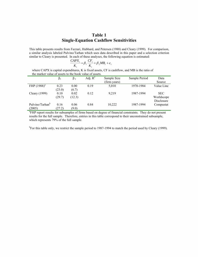
Table 1 Single-Equation Cashflow Sensitivities
This table presents results from Fazzari, Hubbard, and Petersen (1988) and Cleary (1999). For comparison, a similar analysis labeled Pulvino/Tarhan which uses data described in this paper and a selection criterion similar to Cleary is presented. In each of these analyses, the following equation is estimated:
ttt
t
t
t MBK
CFK
CAPXεββ ++= 21
where CAPX is capital expenditures, K is fixed assets, CF is cashflow, and MB is the ratio of the market value of assets to the book value of assets.
β1 β 2 Adj. R2 Sample Size (firm-years)
Sample Period Data Source
FHP (1988)a 0.23 (23.0)
0.00 (6.7)
0.19 5,010 1970-1984 Value Line
Cleary (1999) 0.10 (29.7)
0.02 (12.3)
0.12 9,219 1987-1994 SEC Worldscope Disclosure
Pulvino/Tarhanb (2005)
0.16 (27.2)
0.06 (9.0)
0.84 10,222 1987-1994 Compustat
aFHP report results for subsamples of firms based on degree of financial constraints. They do not present results for the full sample. Therefore, entries in this table correspond to their unconstrained subsample, which represents 79% of the full sample. bFor this table only, we restrict the sample period to 1987-1994 to match the period used by Cleary (1999).

Table 2 Sources and Uses of Investment and Financing Variables
This table describes the variables used to estimate the system described by equation (10) subject to the constraints described by equation (11). Compustat definitions used to construct the variables are described in Table 3.
Variable Name Description Type of Variable
Sources Cash Flow (CF) Internally available cash flow for investment and financing
Exogenous/financing
OTHER The difference between source and use variables that captures miscellaneous sources and uses of funds not explicitly included in the model
Exogenous
ΔLong-term Debt (ΔLTD)
Change in long -term debt Endogenous/financing
ΔShort-term Debt (ΔSTD)
Change in short-term debt Endogenous/financing
Equity Issues (EQUISS)
Dollar value of equity issues Endogenous/financing
Asset Sales (ASALES)
Dollar value of assets sold Endogenous/investment
Uses Share Repurchases (RP)
Dollar value of shares repurchased Endogenous/financing
Dividends (DIV)
Dollar value of dividends paid Endogenous/financing
Capital Expenditures (CAPX)
Dollar value of capital expenditures Endogenous/investment
Acquisitions (ACQUIS)
Dollar value of acquisitions Endogenous/investment
ΔCASH
Change in cash balance Endogenous/financing
Other variables
Market-to Book Ratio (MB)
Ratio of market value of equity to book value of equity
Size (SIZE) Logarithm of total book assets
Exogenous Exogenous

Table 3
Variable Definitions
Variable Description Compustat Pneumonic CASH Cash and equivalents CHE
LTD Long term debt
Long term debt (DLTT)
STD Short term debt Debt in current liabilities (DLC)
EQUISS Sale of common and preferred stock SSTK
ASALES Sale of assets and investments SPPE
CAPX Net capital expenditures Capital expenditures (CAPX)
ACQUIS
Acquisitions
ACQ
RP
Purchase of common and preferred stock
PRSTKC
DIV
Cash dividends
DV
SIZE
Log of total assets
Log of AT
MB
Market-to-book value of assets
(Market value of equity – book value of equity + book value of total assets)/book value of total assets (MKVALF – CEQ + AT)/AT
NWC
Net working capital
(Total current assets (ACT) – cash and equivalents (CHE)) – (Total current liabilities (LCT) – Debt in current liabilities (DLC))
Cash Flow
Internal cash flow net of net interest expense, cash taxes and change in net working capital
EBITDA (OIBDP) – Net interest expense (XINT –IINT) – Cash taxes (TXT – TXDC) – Change in net working capital (ΔNWC)
OTHER
Sources of funds minus uses of funds variables used in the model
(ΔSTD + ΔLTD + Cash Flow + ASALES + EQUISS +) – (CAPX + ACQUIS + RP + DIV + ΔCASH)
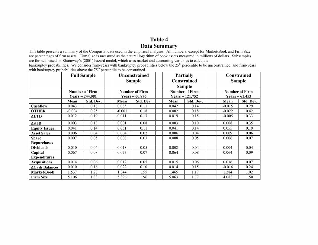
Table 4 Data Summary
This table presents a summary of the Compustat data used in the empirical analyses. All numbers, except for Market/Book and Firm Size, are percentages of firm assets. Firm Size is measured as the natural logarithm of book assets measured in millions of dollars. Subsamples are formed based on Shumway’s (2001) hazard model, which uses market and accounting variables to calculate bankruptcy probabilities. We consider firm-years with bankruptcy probabilities below the 25th percentile to be unconstrained, and firm-years with bankruptcy probabilities above the 75th percentile to be constrained. Full Sample Unconstrained
Sample Partially
Constrained Sample
Constrained Sample
Number of Firm Years = 244,081
Number of Firm Years = 60,876
Number of Firm Years = 121,752
Number of Firm Years = 61,453
Mean Std. Dev. Mean Std. Dev. Mean Std. Dev. Mean Std. Dev. Cashflow 0.043 0.18 0.085 0.11 0.042 0.14 -0.015 0.29 OTHER -0.004 0.25 -0.001 0.18 0.002 0.18 -0.022 0.42 ΔLTD 0.012 0.19 0.011 0.13 0.019 0.15 -0.005 0.33
ΔSTD 0.003 0.18 0.001 0.08 0.003 0.10 0.008 0.35 Equity Issues 0.041 0.14 0.031 0.11 0.041 0.14 0.055 0.19 Asset Sales 0.006 0.04 0.004 0.02 0.006 0.04 0.009 0.06 Share Repurchases
0.007 0.05 0.008 0.03 0.008 0.05 0.006 0.07
Dividends 0.010 0.04 0.018 0.05 0.008 0.04 0.004 0.04 Capital Expenditures
0.067 0.08 0.073 0.07 0.064 0.08 0.064 0.09
Acquisitions 0.014 0.06 0.012 0.05 0.015 0.06 0.016 0.07 ΔCash Balances 0.010 0.16 0.022 0.10 0.014 0.15 -0.016 0.24 Market/Book 1.537 1.28 1.844 1.55 1.465 1.17 1.284 1.02 Firm Size 5.106 1.88 5.896 1.96 5.063 1.77 4.082 1.50
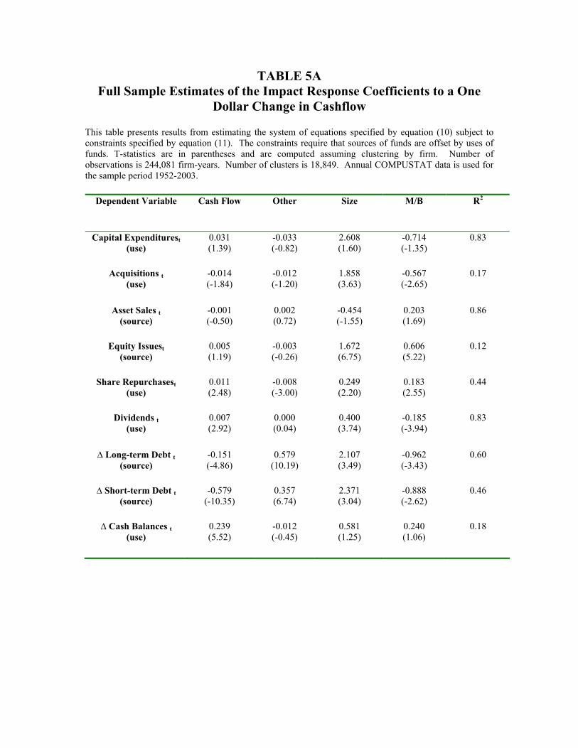
TABLE 5A Full Sample Estimates of the Impact Response Coefficients to a One
Dollar Change in Cashflow
This table presents results from estimating the system of equations specified by equation (10) subject to constraints specified by equation (11). The constraints require that sources of funds are offset by uses of funds. T-statistics are in parentheses and are computed assuming clustering by firm. Number of observations is 244,081 firm-years. Number of clusters is 18,849. Annual COMPUSTAT data is used for the sample period 1952-2003.
Dependent Variable Cash Flow Other Size M/B R2
Capital Expenditurest (use)
0.031 (1.39)
-0.033 (-0.82)
2.608 (1.60)
-0.714 (-1.35)
0.83
Acquisitions t (use)
-0.014 (-1.84)
-0.012 (-1.20)
1.858 (3.63)
-0.567 (-2.65)
0.17
Asset Sales t (source)
-0.001 (-0.50)
0.002 (0.72)
-0.454 (-1.55)
0.203 (1.69)
0.86
Equity Issuest (source)
0.005 (1.19)
-0.003 (-0.26)
1.672 (6.75)
0.606 (5.22)
0.12
Share Repurchasest (use)
0.011 (2.48)
-0.008 (-3.00)
0.249 (2.20)
0.183 (2.55)
0.44
Dividends t (use)
0.007 (2.92)
0.000 (0.04)
0.400 (3.74)
-0.185 (-3.94)
0.83
∆ Long-term Debt t (source)
-0.151 (-4.86)
0.579 (10.19)
2.107 (3.49)
-0.962 (-3.43)
0.60
∆ Short-term Debt t (source)
-0.579 (-10.35)
0.357 (6.74)
2.371 (3.04)
-0.888 (-2.62)
0.46
∆ Cash Balances t (use)
0.239 (5.52)
-0.012 (-0.45)
0.581 (1.25)
0.240 (1.06)
0.18

Table 5B Coefficient Estimates for the System Dynamics Matrix
This table presents results from estimates of the system dynamics matrix, K obtained from estimating the equations specified by equation (10) subject to constraints specified by equation (11). The estimates describe the internal dynamics of the sources and uses variables by specifying how the current state of the sources/uses portfolio depends on its lagged state in the absence of external pressure. In particular, the jth row of K indicates how the current jth sources/uses item is affected by changes in the sources/uses structure last period and the jth column of K describes the rearrangement of the current sources/uses portfolio induced by a partial change in the jth item last period. The diagonal elements of K can be loosely interpreted as own adjustment rates. The smaller in absolute value the jth diagonal element, the less inertia is exhibited in the adjustment of the jth sources/uses variable in question. Since lagged dependent variables are neither sources nor uses in the current period, the constraints require that the reaction of source and use variables are equal and opposite in sign, such that the net effects of lagged dependent variables across the current dependent variables are zero. T-statistics are in parentheses and are computed assuming clustering by firm. Number of clusters is 18,849. Number of observations is 244,081. Annual COMPUSTAT data is used for the sample period 1952-2003.
Dependent Variable
Capital Expendituret-1
Acquisitionst-1 Asalest-1 Equity Issuest-1
Share Repurchasest-1
Dividends t-1 ∆ Long-term Debtt-1
∆ Short-term Debtt-1
∆ Cash Balancest-1
Capital Expenditures
0.873 (6.22)
0.049 (1.72)
0.157 (0.54)
-0.422 (-1.32)
0.137 (2.06)
0.202 (1.15)
0.003 (0.23)
0.013 (1.81)
0.023 (1.65)
Acquisitionst 0.013 (0.78)
0.213 (3.20)
0.090 (1.38)
-0.046 (-1.38)
0.204 (4.03)
0.341 (2.50)
-0.010 (-1.11)
0.006 (1.04)
0.005 (0.95)
Asset Salest 0.074 (2.49)
0.012 (0.96)
0.840 (11.88)
-0.055 (-1.34)
0.045 (0.89)
-0.106 (-1.90)
0.001 (0.17)
0.008 (1.42)
-0.007 (-1.63)
Equity Issuest
0.019 (1.16)
0.049 (1.95)
-0.013 (-0.46)
0.136 (3.49)
0.085 (3.19)
0.020 (0.75)
0.004 (1.20)
-0.002 (-0.83)
0.001 (0.26)
Share Repurchasest
0.003 (0.33)
-0.018 (-1.51)
0.009 (0.58)
0.063 (1.69)
0.583 (9.64)
0.118 (3.17)
-0.002 (-0.64)
0.002 (0.51)
0.011 (2.26)
Dividendst 0.014 (2.50)
0.007 (0.78)
-0.031 (-2.73)
-0.003 (-0.28)
0.030 (2.32)
0.915 (26.31)
0.004 (1.63)
0.004 (1.02)
0.011 (3.46)
∆ Long-term Debtt
0.249 (5.60)
0.128 (1.23)
-0.055 (-0.33)
-0.281 (-2.61)
0.282 (3.99)
0.399 (2.07)
-0.033 (-1.36)
0.051 (3.68)
-0.043 (-1.31)
∆ Short-term Debtt
0.383 (4.61)
-0.001 (-0.02)
-0.182 (-1.56)
-0.108 (-0.60)
0.539 (5.18)
1.106 (7.59)
0.077 (2.35)
-0.026 (-0.85)
-0.004 (-0.06)
∆ Cash Balancest
-0.179 (-4.45)
-0.062 (-1.20)
0.364 (5.66)
0.100 (1.05)
-0.002 (-0.02)
-0.157 (-1.24)
0.053 (2.06)
0.007 (0.22)
-0.101 (-2.41)

Table 6 Cashflow Sensitivities: First Differences versus Levels
This table presents results from estimating the system of equations specified by equation (10) subject to constraints specified by equation (11). T-statistics are in parentheses and are computed assuming clustering by firm. The number of firm-year observations is 237,440 based on annual COMPUSTAT data over the period 1950-2003.
Dependent Variable Cash Flow Coefficients
Using First Differences R2 Cash Flow Coefficients
Using Levels (from Table 5A)
R2
Capital Expenditures t
0.001 (0.20)
0.38 0.031 (1.39)
0.83
Acquisitions t -0.007 (-1.55)
0.25 -0.014 (-1.84)
0.17
Asset Sales t 0.004 (1.93)
0.03 -0.001 (-0.50)
0.86
Equity Issues t -0.001 (-0.30)
0.37 0.005 (1.19)
0.12
Share Repurchases t 0.006 (2.52)
0.15 0.011 (2.48)
0.44
Dividends t 0.001 (0.62)
0.12 0.007 (2.92)
0.83
∆ Long-term Debt t -0.143 (-4.07)
0.67 -0.151 (-4.86)
0.60
∆ Short-term Debt t -0.634 (-11.08)
0.59 -0.579 (-10.35)
0.46
∆ Cash Balances t 0.226 (4.90)
0.45 0.239 (5.52)
0.18

Table 7
Reactions to Cash Flow Changes and the Effects of Financial Constraints
This table presents the coefficients for the Cash Flow variable specified by equation (10), subject to the constraint specified by equation (11). Results are presented for the full sample, and for subsamples constructed on the basis of Shumway’s hazard model, which uses market and accounting variables to predict bankruptcy probabilities. We consider firm years with predicted bankruptcy probabilities below the 25th percentile to be financially unconstrained (FUC), and firm years above the 75th percentile to be financially constrained (FC). Firms in between these two benchmarks are considered to be partially financially constrained (PFC). Shumway-based subsamples contain 58,709, 115,128, and 51,395 firm-years, respectively. The full sample consists of 225,232 firm years. To account for fixed effects, regressions are estimated using first differences and time dummies. Panel A presents coefficient estimates and Panel B presents differences in coefficients across subsamples. Subsample differences are computed by augmenting the system of equations such that the cashflow variable is defined as:
CFDummyFUCCFDummyPFCCF ***** 321 βββ ++ where CF is cashflow, PFC and FUC dummies take on values of 1 if the firm belongs to the appropriate constrained class, and zero otherwise. In the above equation, financially constrained firms (FC) are used as the baseline. A similar approach is followed using the partially financially constrained firms as the baseline to obtain differences between the FUC and PFC subsamples.
PANEL A Dependent Variable
Full Sample Financially Unconstrained
Partially Financially
Constrained
Financially Constrained
Capital Expenditures
0.001 (0.20)
-0.004 (-0.70)
-0.005 (-1.54)
0.003 (0.89)
Acquisitions
-0.007 (-1.55)
-0.029 (-1.28)
-0.018 (-1.90)
-0.003 (-0.70)
Asset Sales
0.004 (1.93)
-0.001 (0.73)
0.001 (0.32))
0.006 (1.79)
Net Change in Investments
-0.007
-0.032
-0.033
-0.006
Equity Issues
-0.001 (0.37)
-0.006 (-1.14)
-0.009 (-2.37)
-0.001 (-0.50)
Share Repurchases
0.006 (2.52)
0.034 (3.49)
0.004 (1.38)
0.002 (0.85)
Dividends
0.001 (0.62)
0.011 (1.90)
0.001 (0.41)
-0.000 (-0.05)
Net Distribution to Shareholders
0.008
0.040
0.014
0.003
Δ Long-Term Debt
-0.143 (-4.07)
-0.352 (-6.02)
-0.170 (-3.57)
-0.073 (-2.14)
Δ Short-Term Debt
-0.634 (-11.08)
-0.380 (-9.58)
-0.580 (-5.66)
-0.703 (-9.60)
Δ Cash Balance
0.226 (4.90)
0.247 (4.08)
0.260 (3.09)
0.228 (3.72)
Change in Leverage
1.00
0.979
1.00
1.00
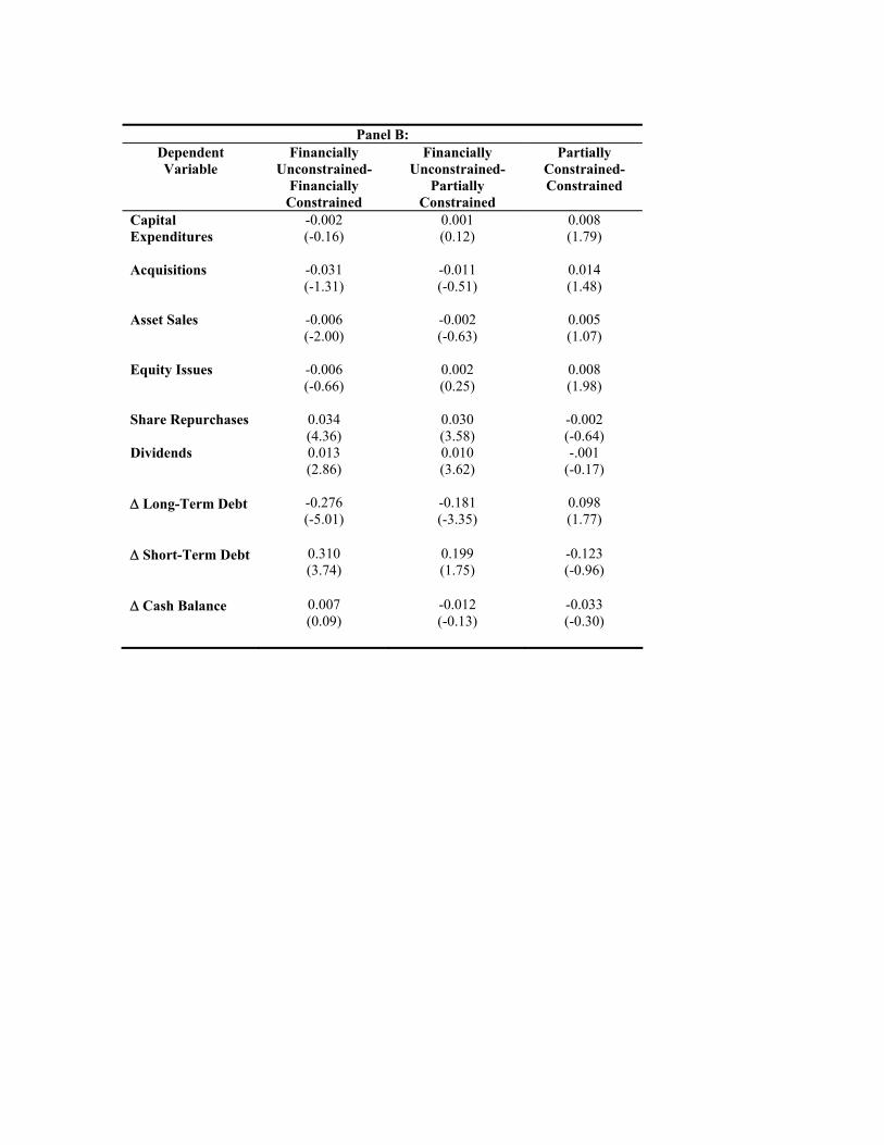
Panel B:
Dependent Variable
Financially Unconstrained-
Financially Constrained
Financially Unconstrained-
Partially Constrained
Partially Constrained- Constrained
Capital Expenditures
-0.002 (-0.16)
0.001 (0.12)
0.008 (1.79)
Acquisitions
-0.031 (-1.31)
-0.011 (-0.51)
0.014 (1.48)
Asset Sales
-0.006 (-2.00)
-0.002 (-0.63)
0.005 (1.07)
Equity Issues
-0.006 (-0.66)
0.002 (0.25)
0.008 (1.98)
Share Repurchases
0.034 (4.36)
0.030 (3.58)
-0.002 (-0.64)
Dividends
0.013 (2.86)
0.010 (3.62)
-.001 (-0.17)
Δ Long-Term Debt
-0.276 (-5.01)
-0.181 (-3.35)
0.098 (1.77)
Δ Short-Term Debt
0.310 (3.74)
0.199 (1.75)
-0.123 (-0.96)
Δ Cash Balance
0.007 (0.09)
-0.012 (-0.13)
-0.033 (-0.30)

Table 8 Testing for Symmetry of Positive and Negative Cash Flow Shocks
This table presents coefficients for the Cash Flow variable for each of the equations in the system specified by equation (10) subject to constraints specified by equation (11). To account for fixed firm and year effects the regressions are estimated using first differences and year dummies. The system (10) is estimated where the right-hand-side includes an interaction variable equal to change in cashflow*DUMMY, where DUMMY equals 1 when change in cashflow is positive, and zero when change in cashflow is negative. Panel A displays the results for the full sample. Panels B, C, and D display the results for the financially unconstrained, partially constrained, and the constrained subsamples.
Panel A: Full Sample N = 225,532
Dependent Variable Positive Cashflow
Shocks t Negative
Cashflow Shocks t Positive-Negative Cashflow Shocks
R2
Capital Expenditures t 0.008 -0.007
0.015 (2.22)
0.38
Acquisitions t -0.009 -0.005
-0.004 (-0.65)
0.25
Asset Sales t
0.007 0.001
0.006 (1.93)
0.03
Equity Issues t -0.000 -0.001
0.001 (0.27)
0.37
Share Repurchases t 0.009 0.003
0.006 (1.83)
0.15
Dividends t 0.009 -0.007
0.016 (5.24)
0.11
∆ Long-term Debtt -0.152 -0.131
-0.021 (-1.17)
0.67
∆ Short-term Debt t -0.607 -0.666
0.059 (1.53)
0.59
∆ Cash Balancest 0.232 0.220
0.012 (0.36)
0.45
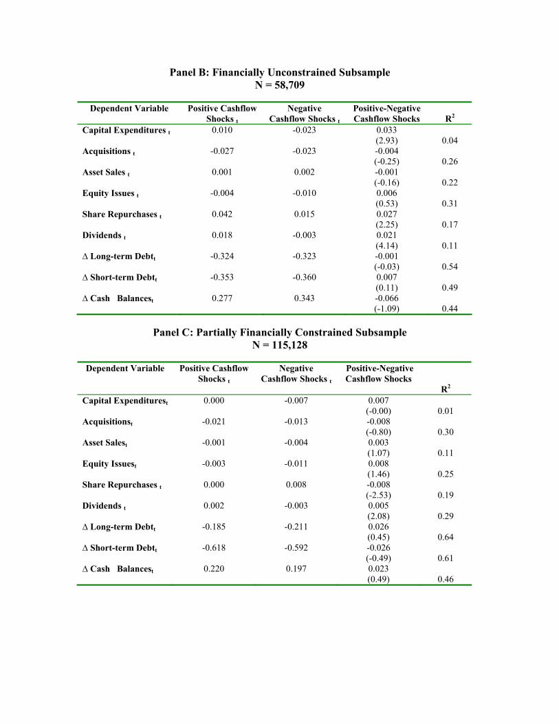
Panel B: Financially Unconstrained Subsample N = 58,709
Dependent Variable Positive Cashflow
Shocks t Negative
Cashflow Shocks t Positive-Negative Cashflow Shocks
R2
Capital Expenditures t 0.010
-0.023
0.033 (2.93)
0.04
Acquisitions t -0.027
-0.023
-0.004 (-0.25)
0.26
Asset Sales t 0.001 0.002
-0.001 (-0.16)
0.22
Equity Issues t -0.004 -0.010
0.006 (0.53)
0.31
Share Repurchases t 0.042
0.015
0.027 (2.25)
0.17
Dividends t 0.018 -0.003
0.021 (4.14)
0.11
∆ Long-term Debtt -0.324
-0.323
-0.001 (-0.03)
0.54
∆ Short-term Debtt -0.353 -0.360
0.007 (0.11)
0.49
∆ Cash Balancest 0.277 0.343
-0.066 (-1.09)
0.44
Panel C: Partially Financially Constrained Subsample
N = 115,128
Dependent Variable Positive Cashflow Shocks t
Negative Cashflow Shocks t
Positive-Negative Cashflow Shocks
R2
Capital Expenditurest 0.000
-0.007
0.007 (-0.00)
0.01
Acquisitionst -0.021
-0.013
-0.008 (-0.80)
0.30
Asset Salest -0.001 -0.004
0.003 (1.07)
0.11
Equity Issuest -0.003 -0.011
0.008 (1.46)
0.25
Share Repurchases t 0.000
0.008
-0.008 (-2.53)
0.19
Dividends t 0.002 -0.003
0.005 (2.08)
0.29
∆ Long-term Debtt -0.185
-0.211
0.026 (0.45)
0.64
∆ Short-term Debtt -0.618 -0.592
-0.026 (-0.49)
0.61
∆ Cash Balancest 0.220
0.197
0.023 (0.49)
0.46
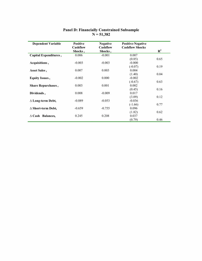
Panel D: Financially Constrained Subsample
N = 51,382
Dependent Variable Positive Cashflow Shocks t
Negative Cashflow Shocks t
Positive-Negative Cashflow Shocks
R2
Capital Expenditures t 0.006 -0.001
0.007 (0.85)
0.65
Acquisitions t -0.003 -0.003
-0.000 (-0.07)
0.19
Asset Sales t 0.007 0.003
0.004 (1.40)
0.04
Equity Issues t -0.002 0.000
-0.002 (-0.67)
0.63
Share Repurchases t 0.003 0.001
0.002 (0.45)
0.16
Dividends t 0.008 -0.009
0.017 (3.09)
0.12
∆ Long-term Debtt -0.089 -0.053
-0.036 (-1.66)
0.77
∆ Short-term Debtt -0.659 -0.755
0.096 (1.82)
0.62
∆ Cash Balancest 0.245 0.208
0.037 (0.79)
0.46


