
elines thetionto the
in
Chapter 31
Calibrating andRecalibrating FOS Data
In This Chapter...Pipeline Calibration Overview / 31-1
Input Files / 31-5CDBS Reference Relations / 31-7
Details of the FOS Pipeline Process / 31-13Paired Aperture Calibration Anomaly / 31-25Recalibrating FOS Data: A Checklist / 31-26
Post-Calibration Output Files / 31-27User Calibrations / 31-29
This chapter describes how data are processed in the standard pipcalibration. The software used in the STScI calibration pipeline is the same acalfos task used to re-calibrate data. Here we will emphasize the calibraprocedures themselves and defer discussions of errors and uncertaintiesnext chapter.
31.1 Pipeline Calibration Overview
The basic steps of the calibration pipeline, calfos, are summarizedFigure 31.1 and Table 31.1.
31 -1

31 -2 Chapter 31 : Calibrating and Recalibrating FOS Data
FOS
/ 31
Figure 31.1: Pipeline Processing by calfos
Subtract Scattered Light SCT_CORRCCS9
Trailer File (.d1h)
Compute Statistical Errors
Convert to Countrate
GIM Correction
Paired Pulse Correction
Subtract Background
DDTHFILE or UDL
CCS7 OFF_CORR
CNT_CORR
SCI (.c4h)
BCK (.c7h)
PPC_CORR
BAC_CORR
Raw Science Images(.d0h, .q0h, .shh, .d1h, .ulh)
CalibratedOutput Files
KeywordSwitches
ProcessingSteps
InputFiles
CCG2
BACHFILE, CCS3,CCS8, and CCS9
DQ2HFILE Initialize Data QualityDQ1HFILE,
ERR_CORR
Flatfield Object and Sky
Subtract Sky
OBJ (.c8h)
FLT_CORR
SKY_CORR
OBJ (.c5h) andSKY (.c6h)
FL1HFILEFL2HFILE
CCS0, CCS2,CCS3, and CCS5
Continued on next page
GMF_CORR

Pipeline Calibration Overview 31 -3
FOS
/ 31
Figure 31.1: Pipeline Processing by calfos (Continued)
Table 31.1: Calibration Steps and Reference Files for FOS PipelineProcessing
Switch Processing StepReferenceFile or Table
ERR_CORR Compute propagated error at each point in spectrum. Error filecalibrated with science file and propagated statistical errors writtento .c2h.
CNT_CORR Convert from raw counts to count rates by dividing each data pointby exposure time and correcting for disabled diodes. Diode numbersare taken from ddthfile or from the unique data log.
ddthfile
OFF_CORR Correct for image motion in the FOS X direction (dispersion)induced by magnetic field. Uses a model of the earth’s magnetic fieldalong with scale factors from table ccs7. This step should be appliedfor observations taken before April 5, 1993, after which the on-boardGIM correction is used.
ccs7
PPC_CORR Correct raw count rates for saturation in detector electronics usingpaired-pulse correction table (coccgr2).
ccg2
BAC_CORR Correct for particle-induced background using default referencebackground (bachfile) if no background spectrum was obtained aspart of the observation.
bachfile
Convert to Absolute Flux
Mode-Dependent Processing
AISHFILE AIS_CORR
MOD_CORRRETHFILECCS4
FLX (.c1h), ERR (.c2h),and CDQ (.cqh)
MOD (.c3h)
Aperture Throughputs and APR_CORRCCSA, CCSB,
Compute Wavelengths
WAV (.c0h)
WAV_CORRCCS6
Time-Dependent Sensitivity TIM_CORRCCSD
CCSC Focus Corrections
Correction

31 -4 Chapter 31 : Calibrating and Recalibrating FOS Data
FOS
/ 31
GMF_CORR If BAC_CORR is set to PERFORM, and the default background file(bachfile) is used, this file can be scaled to the expected mean countrate for the spacecraft geomagnetic position using the ccs8 referencetable and subtracted from the count rate spectra by settingGMF_CORR to PERFORM. Scaled background is written to the.c7h file.
ccs8
SCT_CORR Remove background scattered light. The scattered light isdetermined by calculating the mean value of diodes not illuminatedby the selected grating. This mean is then subtracted from theobserved spectrum. Un-illuminated diodes are found in the CCS9reference table.
ccs9
FLT_CORR Correct for diode to diode sensitivity variations by multiplying by theflatfield response file (fl1hfile). For paired aperture orspectropolarimetry observations, a second flatfield file is used.
fl1hfile,fl2hfile
SKY_CORR If a sky spectrum was observed, the background is subtracted and thesky smoothed using a median and mean filter. Uses filter widths table(ccs3), aperture size table (ccs0), emission line positions (ccs2), andsky shift table (ccs5).
ccs0,ccs2,ccs3,ccs5
WAV_CORR Compute vacuum wavelength scale for each object or sky spectrumusing coefficients (ccs6).
ccs6
APR_CORR Correct for relative aperture throughputs. Object data are normalizedto the reference aperture used to derive the average inverse sensitivityused in AIS_CORR. This step is required if AIS_CORR is used.Additionally, object data are divided to correct for changes inaperture throughput due to changes in OTA focus.
ccsa,ccsb,ccsc
FLX_CORR POLARIMETRY ONLY : Convert from count rate to absolute fluxunits by multiplying by inverse sensitivity curve. Uses inversesensitivity file (iv1hfile) and, for paired aperture orspectropolarimetry, file (iv2hfile).
iv1hfile,iv2hfile
AIS_CORR Convert from count rate to absolute flux units by multiplying byinverse sensitivity curves. This step replaces FLX_CORR and isdifferent in that an average inverse sensitivity, determined fromcalibration of all epochs, is used. APR_CORR must be performed forthis step to have meaning.
aishfile
TIM_CORR Correct for changes in instrument sensitivity over time by dividingthe object data by an appropriate correction factor.
ccsd
MOD_CORR Perform ground software mode dependent corrections fortime-resolved, rapid readout, or spectropolarimetry observations. ForRAPID, write total flux and sum of statistical errors to groups 1 and2 of .c3h file. For PERIOD mode, write pixel-by-pixel averages of allslices to groups 1 and 2 of .c3h file. For spectropolarimetry, datafrom individual waveplate positions is used to make Stokesparameters I, Q, U, and V and linear and circular polarizationposition angle spectra.
ccs4,rethfile
Table 31.1: Calibration Steps and Reference Files for FOS PipelineProcessing (Continued)
Switch Processing StepReferenceFile or Table

Input Files 31 -5
FOS
/ 31
for-
then beS,
064
s
31.2 Input Files
calfos uses three different types of input files:
• Input data files: these are the observation data files, in Generic Edited Inmation Set (GEIS) format, i.e., a multi-group image.
• Reference files (GEIS format images).
• Reference tables (STSDAS tables).
31.2.1 Science Files Required by calfosTable 31.2 lists the science files that are used as required input tocalfos.
Table 31.2: Observation Input Files for calfos
31.2.2 Reference Files and TablesTable 31.1 lists the types of calibration reference files that are used in
pipeline and the information these files contain. Although reference files cagenerated for any combination of NXSTEPS, FCHNL (first channel), NCHNLand OVERSCAN, the routine calibration reference files have a length of 2pixels, corresponding to the standard keyword values:
• NXSTEPS = 4
• FCHNL = 0
• NCHNLS = 512
• OVERSCAN = 5
For other values of FCHNL, NCHNLS, and NXSTEPScalfos interpolatesfrom or resamples the standard reference files.Only OVERSCAN = 5 issupported by FOS calibration. Highly accurate OVERSCAN=1 reference file
File Extension File Contents
.shh and .shd Standard header packet
.ulh and .uld Unique data log
.d0h and .d0d Science data
.q0h and .q0d Science data quality
.x0h and .x0d Science header line
.xqh and .xqd Science header line data quality
.d1h and .d1d Science trailer line
.q1h and .q1d Science trailer line data quality

31 -6 Chapter 31 : Calibrating and Recalibrating FOS Data
FOS
/ 31
es ofs toith
can not be simply extracted from the standard reference files as different valuOVERSCAN produced contributions from different numbers of physical diodethe observed pixels. All FOS calibration observations were made wOVERSCAN=5.
Table 31.3: Reference Tables and Files Required by calfos
HeaderKeyword
Data BaseRelation
FilenameExtension
File Contents
CCS0 cyccs0r .cy0 Aperture areas
CCS1 cyccs1r .cy1 Aperture positions
CCS2 cyccs2r .cy2 Sky emission line positions
CCS3 cyccs3r .cy3 Sky and background filter widths
CCS4 cyccs4r .cy4 Polarimetry parameters
CCS5 cyccs5r .cy5 Sky shift parameters
CCS6 cyccs6r .cy6 Wavelength dispersion coefficients
CCS7 cyccs7r .cy7 GIM correction scale factors
CCS8 cyccs8r .cy8 Predicted background (count rate)
CCS9 cyccs9r .cy9 Un-illuminated diodes for scattered light correction
CCSA cyccsar .cya OTA focus positions for aperture throughputs
CCSB cyccsbr .cyb Aperture throughput coefficients
CCSC cyccscr .cyc Throughput corrections versus focus
CCSD cyccsdr .cyd Instrument sensitivity throughput correction factors
CCG2 coccg2r .cmg Paired-pulse coefficients
BACHFILE cybacr .r0h & .r0d Default background file (count rate)
FLnHFILE cyfltr .r1h & .r1d Flatfield file
IVnHFILE cyivsr .r2h & .r2d Inverse sensitivity file (ergs cm–2 Å–1 count–1 diode–1 )a
a. Note that all references to inverse sensitivity, IVS, in the version 6FOS InstrumentHandbook contain the per diode component of this definition implicitly. The meaning ofIVS is identical in both this document and in theFOS Instrument Handbook.
RETHFILE cyretr .r3h & .r3d Retardation file for polarimetry data
DDTHFILE cyddtr .r4h & .r4d Disabled diode file
DQnHFILE cyqinr .r5h & .r5d Data quality initialization file
AISHFILE cyaisr .r8h & .r8d Average inverse sensitivity file

CDBS Reference Relations 31 -7
FOS
/ 31
ares andachR)
redr
orsky
eseject
tionere
.
onthefor
ients
b-
e istion.
the
etic
bi-
r-
31.3 CDBS Reference Relations
The CDBS relations for the FOS reference files and reference tablesdescribed below. Note that these are relations that point to the reference filetables: they do not contain the data used. Multiple entries are allowed for ereference file or table type which are distinguished by effective (or USEAFTEdate.
• cyccs0r: This table is used to determine the aperture area for paiapertures. If STEP-PATT=OBJ-SKY (or STAR-SKY) is used, it is only fosky subtraction.
• cyccs1r: This table is used to determine which aperture (UPPERLOWER) of a paired aperture was used for observing an object orspectrum.
• cyccs2r:Regions of the sky spectrum known to have emission lines. Thregions are not smoothed before the sky is subtracted from the obspectrum.
The cyccs2r table values were never formally confirmed after science verifica(SV). This had little or no practical impact as, only a few sky observations wtaken, none of which were intended to aid the proposed science.
• cyccs3r: Filter widths used for smoothing the sky or background spectra
• cyccs4r: Polarimetry information regarding waveplate pass directiangles, initial waveplate position angles, the pixel number at whichwavelength shift between the two pass directions is to be determinedcomputing the merged spectrum, and the phase and amplitude coefficfor correction of polarization angle ripple.
• cyccs5r: The shift in pixels to be applied to the sky spectrum before sutraction.
• cyccs6r: Dispersion coefficients to generate wavelength scales. Therone entry for each detector, disperser, aperture, and polarizer combina
• cyccs7r:GIM correction scale factors used to scale the modeled shift ofspectrum due to the earth’s magnetic field.
• cyccs8r: Predicted background count rates as a function of geomagnposition used to scale the background reference file.
• cyccs9r: Un-illuminated diode ranges for each detector and grating comnation. Used to determine the background scattered light.
• cyccsar: List of OTA focus positions versus time. Used to correct for apeture sensitivity dependent on focus position.

31 -8 Chapter 31 : Calibrating and Recalibrating FOS Data
FOS
/ 31
ntseter-
na-
putver
arction.
tec-the
toare
bina-
efluxand
• cyccsbr: As a function of detector and disperser combination, coefficieto normalize aperture throughputs to the reference aperture used to dmine the average inverse sensitivity calibration.
• cyccscr: Throughput corrections versus focus as a function of the combition of detector, disperser, and aperture.
• cyccsdr: As a function of detector and disperser combination, throughcorrection factors to account for changes in instrument sensitivity otime.
• coccg2r: Paired pulse correction table used to correct for non-lineresponse of the diode electronics. Both detectors have the same correconstants, which are time independent. This table is shared with GHRS
• cybacr: This relation is for the background reference files. For each detor there is one file that is used as a default background count rate inevent no background spectra were observed.
• cyfltr: This relation is for the flatfield reference files. These files are usedremove the small scale diode and photocathode non-uniformities. Thereseparate files for each detector, disperser, aperture, and polarizer comtion.
• cyivsr: (polarimetry only)This relation is for inverse sensitivity referencfiles. These files are used to convert corrected count rates to absoluteunits. There are separate files for each detector, disperser, aperturepolarizer combination.
Figure 31.2: Pre-COSTAR Inverse Sensitivity Curves for Blue High DispersionGratings
(erg
s cm
–2 s
–1 Å
–1)/
(cou
nts
s–1 d
iode
–1 )
Wavelength

CDBS Reference Relations 31 -9
FOS
/ 31
Figure 31.3: Pre-COSTAR Inverse Sensitivity Curves for Red High DispersionGratings
Figure 31.4: Post-COSTAR Sensitivity Curves for High Dispersion Gratings
(erg
s cm
–2 s
–1 Å
–1)/
(cou
nts
s–1 d
iode
–1 )
Wavelength
Ave
rage
Sen
sitiv
ity (
coun
ts s
–1 d
iode
)/(e
rg s
–1 c
m–2
Å–1
)
Wavelength

31 -10 Chapter 31 : Calibrating and Recalibrating FOS Data
FOS
/ 31
ari-
tion.te B
Figure 31.5: Post-COSTAR Sensitivity Curves for Low Dispersion Gratings
• cyretr: This relation is for retardation reference files used for spectropolmetric data. The files are used to create the observation matrixf(w). Thereare separate files for each detector, disperser, and polarizer combinaThe three available retardation files for the blue detector and waveplaare plotted in Figure 31.6 with the appropriate disperser shown.
Figure 31.6: Retardation Reference Files
(erg
s cm
–2 s
–1 Å
–1)/
(cou
nts
s–1 d
iode
–1 )
Wavelength

CDBS Reference Relations 31 -11
FOS
/ 31
ed
t theiodeTS-
• cyddtr: This is the relation for the disabled diode files. The table is usonly if the keyword DEFDDTBL = F in the .d0h file. The disabled diodeinformation is also contained in the .ulh file. DEFDDTBL must be set toFfor proper re-calibration of any FOS data!Over the operational lifetime ofthe FOS, 26 FOS/BL and 17 FOS/RD diodes were disabled. Note thadiodes listed in Tables 31.4 and 31.5 are numbered such that the first din the diode array is 0 and the last diode is 511. For use in IRAF and SDAS, the diode number would be the diode number in the table + 1.
.
Table 31.4: Blue Detector Disabled Diodes
DISABLEDDead
Channels
DISABLEDNoisyChannels
DISABLEDCross-Wired
Channels
ENABLEDBut OccasionallyReported Noisy
49 31 268 47 8
101 73 398 55 138
223 144 415 139
284 201 427 209/210
292 218 451 381
409 225 465 421
441 235 472 426
471 241 497
8 16 2 7
Table 31.5: Red Detector Disabled Diodes
DISABLEDDead
Channels
DISABLEDNoisy
Channels
ENABLEDBut OccasionallyReported Noisy
2 110 97 258/259
6 189 114/115 261
29 285 116 268
197 380 142 285
153 381 163 410
212 405 174
289 409 181
308 412 225
486 243
9 8 14

31 -12 Chapter 31 : Calibrating and Recalibrating FOS Data
FOS
/ 31
les.nits.31.2nlyare
nt0 Åod-
F at
adtheTARleBS.
• cyaisr: This is the relation for the average inverse sensitivity reference fiThese files are used to convert corrected count rates to absolute flux uThere is one file for each detector and disperser combination. Figuresand 31.3 show the pre-COSTAR inverse sensitivity for the most commoused gratings for both detectors. The post-COSTAR sensitivity curvesplotted in Figures 31.4 and 31.5
• cypsf: This is the relation for the monochromatic pre-COSTAR poispread functions for the FOS, covering the wavelength range 1200–540for the blue side and 1600–8400 Å for the red side. These PSFs were meled using the TIM software. In Figure 31.7, a sample blue side FOS PS1400 Å is shown.
Figure 31.7: Example of a Pre-COSTAR Point Spread Function for the FOS
• cylsf: This is the relation for the monochromatic pre-COSTAR line sprefunctions for all of the non-occulting FOS apertures computed usingPSFs in cypsf. Figure 31.8 shows a sample monochromatic pre-COSFOS LSF for the blue side4.3 aperture. Pre-COSTAR LSFs are availabat each PSF wavelength. Observation-derived LSFs are not stored in CD

Details of the FOS Pipeline Process 31 -13
FOS
/ 31
e
tions ofrgo
arected.and15
Figure 31.8: Example of a Pre-COSTAR Line Spread Function for the FOS
• cyqinr: This is the relation for the data quality initialization files. Thesfiles were intended to flag intermittent or noisy diodes,but were never keptup to datesince dead diode quality flagging is handled in thecalfospipelinethrough the use of the DDTHFILE dead diode reference file.
31.4 Details of the FOS Pipeline Process
This section describes in detail the STScI pipeline calibration or re-calibra(calfos) procedures. Each step of the processing is selected by the valuekeywordswitchesin the science data header file. All FOS observations undepipeline processing to some extent. Target acquisition and IMAGE mode dataprocessed only through step 6 (paired pulse correction) but are not GIM correACCUM data are processed through step 14 (absolute flux calibration)RAPID, PERIOD, and POLARIMETRY data are processed through step(special mode processing). The steps in the FOS calibration process are:
1. Read the raw data.
2. Calculate statistical errors (ERR_CORR).
3. Initialize data quality.
4. Convert to count rates including dead diode correction (CNT_CORR).
5. Perform GIM correction (OFF_CORR).
6. Do paired-pulse correction (PPC_CORR).

31 -14 Chapter 31 : Calibrating and Recalibrating FOS Data
FOS
/ 31
.
c-
hart
useM.
a.
is
ed byof
00.d to
s are
ctralfromthe
7. Subtract background (BAC_CORR).
8. Subtract scattered light (SCT_CORR).
9. Do flatfield correction (FLT_CORR).
10. Subtract sky (SKY_CORR).
11. Correct aperture throughput and focus effects (APR_CORR).
12. Compute wavelengths (WAV_CORR).
13. Correct time-dependent sensitivity variations (TIM_CORR).
14. Perform absolute calibration (FLX_CORR); superseded by AIS_CORR
15. Do special mode processing (MOD_CORR) if RAPID, PERIOD, or spetropolarimetry.
These steps are described in detail in the following sections. A basic flowcis provided in Figure 31.1.
Note: Fornon-polarimetry cases useonly AIS_CORR; if both are set to PER-FORM, AIS_CORR overrides FLX_CORR as a safeguard. For polarimetryFLX_CORR; here it will override AIS_CORR should both be set to PERFOR
31.4.1 Reading the Raw DataThe raw data, stored in the .d0h file, are the starting point of the pipeline dat
reduction and calibration process. The raw science data are read from thed0hfile and the initial data quality information is read from the .q0h file. If sciencetrailer (.d1h ) and trailer data quality (.q1h ) files exist, these are also read at thtime.
31.4.2 Calculating Statistical Errors (ERR_CORR)The noise in the raw data is photon (Poisson) noise and errors are estimat
simply calculating the square root of the raw counts per pixel. An error valuezero is assigned to filled data, i.e., pixels that have a data quality value of 81
For all observing modes except polarimetry, an error value of zero is assignepixels that have zero raw counts. Polarimetry data that have zero raw countassigned an error value of one.
From this point on, the error data are processed in lock-step with the spedata. Errors caused by sky and background subtraction, as well as thoseflatfields and inverse sensitivity files, are not included in the error estimate. Atend of the processing, the calibrated error data will be written to the.c2h file.
1. Data quality values are described in Table 30.2.

Details of the FOS Pipeline Process 31 -15
FOS
/ 31
iess
inndfor
160,ining
otheredten
, butdis-
afterdesfile.
ingero.
dd
ead
ed isacheral15).
nalrectdese
31.4.3 Data Quality InitializationThe initial values of the data quality information are the data quality entr
from the spacecraft as recorded in the.q0h file. This step of the processing addvalues from the data quality reference files to the initial values in the.q0h file.The routine uses the data quality initialization reference file DQ1HFILE listedthe .d0h file. A second file, DQ2HFILE, is necessary for paired-aperture aspectropolarimetry observations. These reference files contain flagsintermittent noisy and dead channels (data quality values 170 andrespectively). The data quality values are carried along throughout the remaprocessing steps where subsequent routines add values corresponding toproblem conditions.Only the highest (most severe) data quality value is retainfor each pixel. At the end of the processing the final data quality values are writto the .cqh file.
The noisy and dead channels in the data quality files were often out of datethe dead diode table (DDTHFILE) contains the most accurate list of dead andabled diodes. Noisy diodes are not flagged in routine processing. Normally,three reports of noisy activity an offending diode was disabled. As a result, diothat had fewer than three reports as noisy are not flagged in the data quality
31.4.4 Conversion to Count Rates (CNT_CORR)At this step, the raw counts per pixel are converted to count rates by divid
by the exposure time of each pixel. Filled data (data quality = 800) are set to zA correction for disabled diodes is also included at this point.If the keywordDEFDDTBL in the .d0h file is set to TRUE, the list of disabled diodes is reafrom the unique data log (.ulh ) file. Otherwise the list is read from the disablediode reference file, DDTHFILE, named in the .d0h file. In pipeline calibrationthe DDTHFILE was more commonly used for the disabled diode information.
For re-calibration purposes, DEFDDTBL should always be set toFALSE sothat the FOS closeout calibration dead diode tables are used for the proper ddiode correction.
The actual process by which the correction for dead diodes is accomplishas follows. First, recall that because of the use of the OVERSCAN function, epixel in the observed spectrum actually contains contributions from sevneighboring diodes (see “Data Acquisition Fundamentals” on page 29-Therefore, if one or more particular diodes out of the group thatcontributed toagiven output pixel is dead or disabled, there will still be some amount of sigdue to the contribution of the remaining live diodes in the group. We can corthe observed signal in that pixel back to the level it would have had if all diowere live; to do this, we divide by the relative fraction of live diodes. Th

31 -16 Chapter 31 : Calibrating and Recalibrating FOS Data
FOS
/ 31
ead
areedsvenuality
the
rdforeme
d oncraft.ated in
thescaleo the
bitaloup.egere to
eline
ayr ay at
corrected pixel value is zero if all the diodes that contribute to that pixel are dor disabled, otherwise, the value is given by the equation:
Where:
• corr – is the corrected pixel value.
• obs – is the observed pixel value.
• total – is the total number (live + dead) of diodes.
• dead – is the number of dead or disabled diodes.
This correction to the signal is applied at the same time the raw datadivided by exposure time. If the fraction of dead diodes for a given pixel exce50%, then a data quality value of 50 is assigned. If all of the diodes for a gipixel are dead, both the data and error values are set to zero and a data qvalue of 400 is assigned.
The count rate spectral data are written to the .c4h file at this point. Note thatthe S/N and the computed statistical errors in a given pixel are appropriate toactually observed, not the corrected, count rate.
31.4.5 GIM Correction (OFF_CORR)Data obtained prior to April 5, 1993, do not have an onboa
geomagnetic-induced image motion (GIM) correction applied, and thererequire a correction for GIM in the pipeline calibration. Note that there are soobservations obtained after April 5, 1993, that donot have onboard GIMcorrection, because the application of the onboard GIM correction dependewhen the proposal was completely processed for scheduling on the spaceReference to keywords YFGIMPEN and YFGIMPER, respectively, indicwhether onboard GIM correction was enabled and whether any error occurreits implementation. The GIM correction is determined by scaling a model ofstrength of the geomagnetic field at the location of the spacecraft. The modelfactors are read from the CCS7 reference table. The correction is applied tspectral data, the error data, and the data quality values.
A unique correction is determined for each data group based on the orposition of the spacecraft at the mid-point of the observation time for each grWhile the correction is calculated to sub-pixel accuracy, it is applied as an intvalue and is therefore accurate only to the nearest integral pixel. This is donavoid resampling the data in the calibration process. Furthermore, the pipcorrection (OFF_CORR) is applied only in thex-direction (i.e., the dispersiondirection).
The correction is applied by simply shifting pixel values from one arrlocation to another. As a typical example, if the amount of the correction foparticular data group is calculated to be +2.38 pixels, the data point originall
corr obstotal
total dead–( )------------------------------------=

Details of the FOS Pipeline Process 31 -17
FOS
/ 31
5,this
o and
achly a
cted
tn beto
alwith
ongtheof
d is
deads of
itiesever
the
pixel location 1 is shifted to pixel 3, pixel 2 shifted to pixel 4, pixel 3 to pixeland so on. Pixel locations at the ends of the array that are left vacant byprocess (e.g., pixels 1 and 2 in the example above) are set to a value of zerare assigned a data quality value of 700.
Special handling is required for data obtained in ACCUM mode since edata frame contains the sum of all frames up to that point. In order to appunique correction to each frame, data taken in ACCUM mode are firstunraveledinto separate frames. Each frame is then corrected individually, and the correframes are recombined.
The pipeline processingGIM correction (OFF_CORR) is not applied to targeacquisition data, image mode data, and polarimetry data. The correction caapplied to IMAGE modespectraldata by setting header keyword OFF_CORRPERFORM prior to runningcalfos.
The onboard GIM correction is applied on a much finer grid than integrpixels and is made within the FOS so that data are recorded by the detectorthe corrections already included. The onboard GIM correction is applied alboth the direction of the diode array and in the perpendicular direction. Inx-direction the onboard GIM correction is applied in units of 1/32 of the widththe diodes and in they-direction in units of 1/256 of the diode height.
The onboardGIM correction is calculated and applied every 30 seconds, anapplied to all observations except for ACQ/PEAK observations.
31.4.6 Paired Pulse Correction (PPC_CORR)This step corrects the data for saturation in the detector electronics. The
time constants q0, q1, and F are read from the reference table CCG2. The valuethese dead time constants in the CCG2 table are q0 = 9.62e-6 seconds,q1 = 1.826e-10 sec2/counts, and F = 52,000 counts per second. These quantwere determined in laboratory measurements prior to launch and were nmodified (FOS ISRs 25 and 45). The following equation is used to estimatetrue count rate:
Where:
• x – is the true count rate.
xy
1 yt–( )------------------=

31 -18 Chapter 31 : Calibrating and Recalibrating FOS Data
FOS
/ 31
ws:
perd
d 10imits/sec-
andlue of
,000
not
fromwith
oundasedn, isscaled
badetry
hethingy aionslue of
• y – is the observed count rate.
• t – is q0 for y less than or equal to F.
• t – is q0 + q1 * (y-F) for y greater than F.
The values of these different saturation limits in the CCG2 table are as follo
• Observed count rates greater than the saturation limit of 57,000 countssecond (and recorded in thecalfos processing log) are set to zero anassigned a data quality value of 300.
• All observed count rates that are between this severe saturation limit ancounts/second are corrected, but those lying between the predefined lof large (55,000 counts/second) and severe saturation (57,000 countsond) are assigned a data quality value of 190.
• Those that lie between the limits of moderate (52,000 counts/second)large (55,000 counts/second) saturation are assigned a data quality va130, and the paired pulse correction is applied.
• Count rates between the threshold value (10 counts/second) and 52counts/second have the paired pulse correction applied.
• Data with count rates below this threshold value (10 counts/second) dohave any paired-pulse correction.
31.4.7 Background Subtraction (BAC_CORR)This step subtracts the background (i.e., the particle-induced dark count)
object and sky (if present) spectra. If no background spectrum was obtainedthe observation (the situation for nearly all FOS exposures), a default backgrreference file, BACHFILE, which is scaled to a mean expected count rate bon the geomagnetic position of the spacecraft at the time of the observatioused. The scaling parameters are stored in the reference table CCS8. Thebackground reference spectrum is written to the .c7h file for later examination.
If an observed background was used (rarely the case), it is first repaired;points (i.e., points at which the data are flagged as lost or garbled in the telemprocess) are filled by linearly interpolating betweengood neighbors. Next, thebackground is smoothed with a median filter, followed by a mean filter. Tmedian and mean filter widths are stored in reference table CCS3. No smoois done to the background reference file, if used, since the file is alreadsmoothed approximation to the background. Spectral data at pixel locatcorresponding to repaired background data are assigned a data quality va120. Finally, the repaired background data are subtracted.
Although this is called background subtraction, it is really adark countsubtraction.
Details of the FOS Pipeline Process 31 -19
FOS
/ 31
s oftings.
ngsy to.6).12,the
ghtratedingf a
deritVALd infile.
od, aa
s thethe
tonsthe
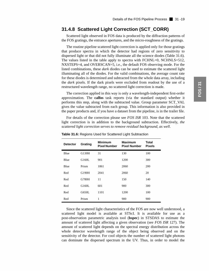
31.4.8 Scattered Light Correction (SCT_CORR)Scattered light observed in FOS data is produced by the diffraction pattern
the FOS gratings, the entrance apertures, and the micro-roughness of the gra
The routine pipeline scattered light correction is applied only for those gratithat produce spectra in which the detector had regions of zero sensitivitdispersed light or that did not fully illuminate all the science diodes (Table 31The values listed in the table apply to spectra with FCHNL=0, NCHNLS=5NXSTEPS=4, and OVERSCAN=5, i.e., the default FOS observing mode. Forlisted combinations, thesedark diodes can be used to estimate the scattered liilluminating all of the diodes. For the valid combinations, the average countfor these diodes is determined and subtracted from the whole data array, incluthe dark pixels. If the dark pixels were excluded from readout by the use orestructured wavelength range, no scattered light correction is made.
The correction applied in this way is only a wavelength-independent first-orapproximation. Thecalfos task reports (via the standard output) whetherperforms this step, along with the subtracted value. Group parameter SCT_gives the value subtracted from each group. This information is also providethe paper products and, if you have a dataset from the pipeline, is in the trailer
For details of the correction please seeFOS ISR103. Note that the scatteredlight correction is in addition to the background subtraction. Effectively,thescattered light correction serves to remove residual background, as well.
Since the scattered light characteristics of the FOS are now well understoscattered light model is available at STScI. It is available for use aspost-observation parametric analysis tool (bspec) in STSDAS to estimate theamount of scattered light affecting a given observation (seeFOS ISR127). Theamount of scattered light depends on the spectral energy distribution acroswhole detector wavelength range of the object being observed and onsensitivity of the detector. For cool objects the number of scattered light phocan dominate the dispersed spectrum in the UV. Thus, in order to model
Table 31.6: Regions Used for Scattered Light Subtraction
Detector GratingMinimumPixel Number
MaximumPixel Number
TotalPixels
Blue G130H 31 130 100
Blue G160L 901 1200 300
Blue Prism 1861 2060 200
Red G190H 2041 2060 20
Red G780H 11 150 140
Red G160L 601 900 300
Red G650L 1101 1200 100
Red Prism 1 900 900
31 -20 Chapter 31 : Calibrating and Recalibrating FOS Data
FOS
/ 31
as tojectting
tureskythedare
eldFOS
use
amerum ist intableskysky
o thatum isbjecttned a
sizeS5.
one andere
ionsons
scattered light in the FOS appropriately, the red part of the source spectrum hbevery wellknown. For an atlas of predicted scattered light as a function of obtype and FOS disperser and additional guidelines for modeling FOS grascatter withbspec, seeFOS ISR151.
31.4.9 Flatfield Correction (FLT_CORR)This step removes the diode-to-diode sensitivity variations and fine struc
(typically on size scales of ten diodes or less) from the object, error, andspectra by multiplying each by the inverse flatfield response as stored inFL1HFILE reference file. A second flatfield file, FL2HFILE, is required for paireaperture or spectropolarimetry observations. No new data quality valuesassigned in this step.
Different locations on the FOS photocathodes displayed quite different flatficharacteristics so that FOS flats were aperture-dependent. Additionally,flatfields for some dispersers were quite time-variable. Care must be taken tothe correct flatfield reference file for the date and aperture of observation.
31.4.10 Sky Subtraction (SKY_CORR)If the sky was observed, the flatfielded sky spectrum is repaired in the s
fashion as described above for an observed background spectrum. The spectthen smoothed once with a median filter and twice with a mean filter, excepregions of known emission lines, which are masked out. The CCS2 referencecontains the pairs of starting and ending pixel positions for masking theemission lines. The sky spectrum is then scaled by the ratio of the object andaperture areas, and then shifted in pixel space (to the nearest integer pixel) sthe wavelength scales of the object and sky spectra match. The sky spectrthen subtracted from the object spectra and the resulting sky-subtracted ospectrum is written to the .c8h file. Pixel locations in the sky-subtracted objecspectrum that correspond to repaired locations in the sky spectrum are assigdata quality value of 120.
This routine requires table CCS3 containing the filter widths, the aperturetable CCS0, the emission line position table CCS2, and the sky shift table CC
For OBJ-SKY (or STAR-SKY) observations, half the integration time is spentthe sky. The only science observations made of the sky were taken by mistakwere not required for proposal science. Additionally, the CCS2 table values wnever confirmed.
Note that—especially for extended objects—paired aperture observatcould be obtained in the so-called “OBJ-OBJ” mode, in which no sky subtractiwere performed (see “Paired Aperture Calibration Anomaly” on page 31-25).

Details of the FOS Pipeline Process 31 -21
FOS
/ 31
rentstablein
o
rst
mustlues
de,ngths
as are
R in
31.4.11 Computing the Wavelength Scale(WAV_CORR)
A vacuumwavelength scale atall wavelengths is computed for each object osky spectrum. Wavelengths are computed using dispersion coefficicorresponding to each grating and aperture combination stored in referenceCCS6.Corrections for telescope motion or motion of the Earth are not madethe standard pipeline calibration.The computed wavelength array is written tthe .c0h file.
For the gratings the wavelengths are computed as follows:
For the prism, wavelengths are computed as:
Where:
• l(p) – are the dispersion coefficients in table CCS6.
• x – is the position (in diode units) in the object spectrum, where the fidiode is indexed as 0.
• x0 – is a scalar parameter also found in table CCS6.
Note that the above equations determine the wavelength at each diode. Thisbe converted to pixels using NXSTEPS. For example, if NXSTEPS=4, the vafor x are given as 0, 0.25, 0.5, 0.75, 1, etc., for pixels 1, 2, 3, 4, 5, etc.
For multigroup data, as in either rapid-readout or spectropolarimetry mothere are separate wavelength calculations for each group. These wavelemay be identical or slightly offset, depending on the observation mode.
31.4.12 Aperture Throughput Correction(APR_CORR)
This calibration step consists of two parts: normalizing throughputs toreference aperture and correcting throughputs for focus changes. Both steprelevant only if the average inverse sensitivity files are used, see AIS_CORthe next sub-section.
λ Å( ) l p( ) xp×
p 0=
3
∑=
λ Å( ) l p( )x x0–( )p
---------------------p 0=
4
∑=

31 -22 Chapter 31 : Calibrating and Recalibrating FOS Data
FOS
/ 31
. Tot beinedisThethe
d fort of
n ofThisARoper
rseergd.nch
996.and
nd,RR
rsedtion
ndrrectdingatedn
end
orverye, in.
Each aperture affected the throughput of light onto the photocathodeprepare the object data for absolute flux calibration, the object data musnormalized to the throughput as would be seen through a pre-determreference aperture (the4.3 aperture is always used). The normalizationcalibrated as a second-order polynomial and is a function of wavelength.polynomial is evaluated over the object wavelength range and divided intoobject data. The coefficients are found in the CCSB reference table.
Once the object data has been normalized, the throughput is compensatevariations in sensitivity due to focus changes. The CCSA table contains a lisdates and focus values. The sensitivity variation is modeled as a functiowavelength and focus, the coefficients of which are found in the CCSC table.model is evaluated and divided into the object data. (Although post-COSTfocus-dependent corrections are unity, this step still must be performed for prcalibration).
31.4.13 Absolute Flux Calibration (AIS_CORR andFLX_CORR)
This step multiplies object (and error) spectra by the appropriate invesensitivity vector to convert from count rates per pixel to absolute flux units (s–1 cm–2 Å–1). Two different methods of performing this calibration were useThe pipeline used the so-called FLX_CORR method from the time of HST lauto March 19, 1996. The pipeline processing method, fornon-polarimetricobservations, was changed to the AIS_CORR method on March 19, 1AIS_CORR calibration files are available for all FOS observing epochsAIS_CORR is the only recommendedmethod for the flux calibration (orre-calibration) of non-polarimetric FOS observations. On the other haspectropolarimetric measures will continue to be processed via the FLX_COmethod.
AIS_CORR:This step is functionally no different than FLX_CORR except fothe way in which absolute flux is calibrated. The absolute flux calibration is baon data from all calibration observation epochs. An average sensitivity funcfor the entire pre- or post-COSTAR period for the4.3 reference aperture iscontained in the AISHFILE reference file for each combination of detector adisperser. As necessary, TIM_CORR factors (see following sub-section) cothe sensitivity to the date of observation and APR_CORR factors (see precesub-section) correct for the throughput of the aperture employed. The calibrspectral data are written to the .c1h file, and the calibrated error data are writteto the .c2h file. The final data quality values are written to the .cqh file.
FLX_CORR: Now used for spectropolarimetry flux calibration only. Thinverse sensitivity data are read from the IV1HFILE reference file. A secoinverse sensitivity file, IV2HFILE, is required for paired-aperturespectropolarimetry observations. Individual reference files are required for ecombination of detector, disperser, and aperture. Time-dependencies arprinciple, tracked via multiple reference files with different USEAFTER dates

Details of the FOS Pipeline Process 31 -23
FOS
/ 31
erotedn
heuxtorgthare
etrythisa
reach
on.
an
ins the
For both flux calibration methods, points where the inverse sensitivity is z(i.e., not defined) are flagged with a data quality value of 200. The calibraspectral data are written to the .c1h file, and the calibrated error data are writteto the .c2h file. The final data quality values are written to the .cqh file.
31.4.14 Time Correction (TIM_CORR)This step corrects the absolute flux for variations in sensitivity of t
instrument over time and is an important component of the AIS_CORR flcalibration. The correction factor is a function of time and wavelength. The facis calculated by linear interpolation for the observation time and wavelencoverage. The factor is divided into the object absolute flux. The coefficientsfound in table CCSD. TIM_CORR is used only with AIS_CORR calibration.
This is the final step of processing for ACCUM mode observations.
31.4.15 Special Mode Processing (MOD_CORR)Data acquired in the rapid-readout, time-resolved, or spectropolarim
modes receive specialized processing in this step. All data resulting fromadditional processing are stored in the .c3h file. See the discussions of output datproducts for each of these modes on pages 30-40, 30-42, and 30-46.
RAPID Mode: For RAPID mode, the total flux, integrated over all pixels, foeach readout is computed. The sum of the statistical errors in quadrature forframe is also propagated. The following equations are used in the computati
Where:
• f(x,F) – is the flux in pixelx and readoutF.
• ef(x,F) – is the associated error in the flux for pixelx and readoutF.
• sum(F) – is the total flux for readoutF.
• errsum(F)– is the associated error in the total flux for the readoutF.
• NDAT – is the total number of pixels in the readoutF.
• good– is total number of good pixels, i.e., pixels with data quality less th200.
The output .c3h file contains two data groups, where the number of pixelseach group is equal to the number of original data frames. Group 1 contain
sum F( ) f x F,( )x 1=
NDAT
∑ NDAT
good----------------
=
errsum F( ) e f2
x F,( )x 1=
NDAT
∑ NDAT
good----------------
×=

31 -24 Chapter 31 : Calibrating and Recalibrating FOS Data
FOS
/ 31
ford
d Vtion
uted.r thed for
se forn the
cu-
total flux for each frame, where pixel 1 is the sum for frame 1, pixel 2 the sumframe 2, etc. Group 2 of the .c3h file contains the corresponding propagateerrors.
POLARIMETRY Mode: For the POLARIMETRY mode, the data fromindividual waveplate positions are combined to calculate the Stokes I, Q, U, anparameters, as well as the linear and circular polarizations and polarizaposition angle spectra (for details of calculating the Stokes parameters seeFOSISR078). Four sets of Stokes parameter and polarization spectra are compThe first two sets are for each of the separate pass directions, the third focombined pass direction data, and the fourth for the combined data correcteinterference and instrumental orientation.
PERIOD Mode: For PERIOD mode, the pixel-by-pixel average of all slice(NSLICES separate memory locations) and the differences from the averageach slice of the last frame are computed. The following equations are used icomputation:
Where
• NSLICES – is the number of slices.
• f(x,L) – is the flux in sliceL at pixelx.
• ef(x,L) – is the error associated with the flux in slice L at pixelx.
• average(x) – is the average flux of all slices at the pixelx.
• errave(x) – is the error associated with the average flux at pixelx.
• good(x)– is the total number of good values, i.e., data quality <200, acmulated at pixelx.
• diff(x,L) – is the flux difference at pixel x between sliceL and the average.
• errdiff(x,L) – is the error associated with the flux difference.
average x( )
f x L,( )L 1=
NSLICES
∑good x( )
--------------------------------------
=
errave x( )
ef x l,( )( )2
L 0=
NSLICES 1–
∑
good x( )---------------------------------------------------------------=
diff x L,( ) f x L,( ) average x( )–=
errdiff x L,( ) ef x L,( )2 errave x( )2+( )=
Paired Aperture Calibration Anomaly 31 -25
FOS
/ 31
ntainsce.
eed
rtureY,ctsthisvereachion ofdate.
iredn theven ifr toiredingy
key-
parate
verytionforethernal
d only
The first two data groups of the output .c3h file contain the average flux andthe associated errors, respectively. Each subsequent pair of data groups cothe difference from the average and the corresponding total error for each sli
31.5 Paired Aperture Calibration Anomaly
Any HST data taken with a paired aperture prior to January 1, 1995 may nmanual editing of certain .d0 header fields prior to recalibration withcalfos.
Several programs used both the upper and lower portions of a paired apewith Exposure Logsheet (or RPS2) entries of STEP-PATT=STAR-SKOBJ-OBJ, or OBJ-SKY in order to sample different portions of extended objein alternating 10-second dwells throughout an exposure. The diagnosis ofproblem is slightly complicated, but in the following, please realize that whene“chopping” between apertures was invoked, the data recorded throughaperture segment were always recorded separately so that correct calibratthe data from each aperture segment is possible after the manual header up
Prior to January 1, 1995 important keywords in the headers of all FOS paaperture exposures for STEP-PATT not equal to SINGLE were constructed oassumption that SKY was sampled in one aperture segment. This occurred eSTEP-PATT=OBJ-OBJ had been specified in the logsheet. Additionally, prioFebruary 1, 1994 the only way to obtain spectra with both segments of the paapertures in this alternating fashion was to specify the potentially misleadSTEP-PATT=STAR-SKY. Naturally,calfos calibrates these exposures as if sksubtraction is intended and the final.c1 file contains the difference betweennominal default star and sky apertures.
The simplest approach to correcting this problem is to change the YSTEPnwords (i.e., YSTEP1, YSTEP2, etc) from “SKY” to “OBJ.” Values of “NUL” or“BCK” should not be changed. Modern versions ofcalfos (revised afterJanuary 1, 1995) will process these updated data correctly and produce secalibrated spectra for the two aperture segments.
As a general rule, no sky subtraction observations wereintendedby anyobserver in the FOS science program after SV ended (January 1, 1992). On afew occasions OBJ-SKY observations were obtained through implementaerror when only OBJ (i.e., STEP-PATT=SINGLE) was intended. Particularlyextended targets, you should broadly assume that any SKY observation, whexplicitly requested in the logsheet STEP-PATT or not, may contain additiospectra from nearby regions of an extended source and should be recalibrateafter header update.

31 -26 Chapter 31 : Calibrating and Recalibrating FOS Data
FOS
/ 31
.
.
ny
rtask
derAR
cali-t on
efilesiewleteceunc-
ra-
nval-1.5
yr to-now
es.isset
data,d in
duced
31.6 Recalibrating FOS Data: A Checklist
You will use the IRAF/STSDAS taskcalfos. to recalibrate your FOS spectraThis task sequentially performs each step described in the preceding section
Here is a checklist of things that you should routinely do to re-calibrate aFOS exposure:
1. Add new or updated keywords: The first thing to do is make sure that youdata have all the required keywords in their headers. The STSDASaddnewkeyswill update the headers of your .d0h files accordingly. Thistask insures that the AIS flux calibration method keywords are in the heaand also adds the scattered light correction keyword to older pre-COSTfiles. Note that a default set of reference filenames is used for the newbration switch keywords - you must update these as part of the next pointhis checklist.
2. Get correct reference file names: Next you must determine which are thcorrect reference files to use. You can determine the correct referenceand tables to use for re-calibration of any exposure by using the StarVFOS calibration reference file screen (see section 1.3 for a compdescription of this procedure). Alternatively, the FOS WWW ReferenFile Guides provide a listing of recommended FOS reference files as a ftion of observing epoch for each type of reference file or table.
3. Update header files: In order to recalibrate FOS data using updated calibtion files, you need to edit the header of the original science data, .d0h ,with the taskchcalpar and replace the names of the original calibratiofiles with those of the new ones. If required, you should also update theues of YSTEPn for paired aperture exposures as described in section 3
4. Set DEFDDTBL to “F” (false): As noted earlier, some header files mahave had the Default Dead Diode Table keyword set to TRUE in ordeuse the .udl file to specify the list of dead diodes for original pipeline processing. Since a complete history of dead diode occurrence dates isavailable, only the DDTHFILE should now be used to identify dead diodUnder no circumstances should DEFDDTBL be set to “T”. Naturally, italso a good idea to make sure that all other calibration switches areproperly at this point.
5. Run the calfos calibration routine: calfoswill create new calibrated outputfiles with the same suffixes as the originally delivered data, namely .cnhand .cnd (n=0...8).
If you are concerned about any aspect of the appearance of your calibratedyou should compare the final data with flatfield (and other) reference files usethe data reduction process to make sure that spurious features were not introthrough improper data handling in the pipeline or in your recalibration.

Post-Calibration Output Files 31 -27
FOS
/ 31
in
o notcan
, weiting
31.7 Post-Calibration Output Files
The several types of calibrated output files produced bycalfos are listed inTable 31.7. More detailed descriptions of each type of file are providedChapter 30.
Table 31.7: Output Calibrated FOS Data Files
If the reference files and reference tables used in the pipeline processing dreflect the actual instrument performance, calibration errors can occur, whichlead to artificial features in the calibrated science data. In the next chapteraddress a variety of sources of error in FOS calibration and assess limaccuracies in the STScI instrument calibration.
Filename Extension File Contents
.c0h and .c0d Calibrated wavelengths
.c1h and .c1d Calibrated fluxes
.c2h and .c2d Calibrated statistical error
.c3h and .c3d Special mode data
.cqh and .cqd Calibrated data quality
.c4h and .c4d Count rate object and sky spectra
.c5h and .c5d Flatfielded object count rate spectrum
.c6h and .c6d Flatfielded sky count rate spectrum
.c7h and .c7d Background count rate spectrum
.c8h and .c8d Flatfielded and sky subtracted object count rate spectrum

31 -28 Chapter 31 : Calibrating and Recalibrating FOS Data
FOS
/ 31
Figure 31.9: Partial Sample Post-COSTAR FOS .c1h Header
GCOUNT = 77 / / FOS DATA DESCRIPTOR KEYWORDSINSTRUME= 'FOS ' / instrument in useROOTNAME= 'Y3JK0709T ' / rootname of the observation setFILETYPE= 'FLX ' / file typeBUNIT = 'ERGS/CM**2/S/A' / brightness units
/ CALIBRATION FLAGS AND INDICATORSGRNDMODE= 'RAPID-READOUT ' / ground software modeDETECTOR= 'BLUE ' / detector in use: amber, blueAPER_ID = 'B-2 ' / aperture idPOLAR_ID= 'C ' / polarizer idPOLANG = 0.0 / initial angular position of polarizerFGWA_ID = 'H13 ' / FGWA idFCHNL = 0 / first channelNCHNLS = 512 / number of channelsOVERSCAN= 5 / overscan numberNXSTEPS = 4 / number of x stepsYFGIMPEN= T / onboard GIMP correction enabled (T/F)YFGIMPER= 'NO ' / error in onboard GIMP correction (YES/NO)
/ CALIBRATION REFERENCE FILES AND TABLESDEFDDTBL= F / UDL disabled diode table usedBACHFILE= 'yref$b3m1128my.r0h' / background reference header fileFL1HFILE= 'yref$e7813577y.r1h' / first flat-field header fileFL2HFILE= 'N/A ' / second flat-field header fileIV1HFILE= 'yref$e3h14503y.r2h' / first inverse sensitivity header fileIV2HFILE= 'N/A ' / second inverse sensitivity header fileAISHFILE= 'yref$fac08361y.r8h' / average inverse sensitivity header fileRETHFILE= 'N/A ' / waveplate retardation header fileDDTHFILE= 'yref$d9h1244ay.r4h' / disabled diode table header fileDQ1HFILE= 'yref$b2f1306ry.r5h' / first data quality initialization header fileDQ2HFILE= 'N/A ' / second data quality initialization header fileCCG2 = 'mtab$a3d1145ly.cmg' / paired pulse correction parameters tableCCS0 = 'ytab$a3d1145dy.cy0' / aperture parametersCCS1 = 'ytab$aaj0732ay.cy1' / aperture position parametersCCS2 = 'ytab$a3d1145fy.cy2' / sky emission line regionsCCS3 = 'ytab$a3d1145gy.cy3' / bkg and sky filter widthsCCS4 = 'ytab$e5v13262y.cy4' / polarimetry parametersCCS5 = 'ytab$a3d1145jy.cy5' / sky shiftsCCS6 = 'ytab$e5v11576y.cy6' / wavelength coefficientsCCS7 = 'ytab$ba910502y.cy7' / GIMP correction scale factorsCCS8 = 'ytab$ba31407ly.cy8' / predicted background count ratesCCS9 = 'ytab$e3i09491y.cy9' / scattered light parametersCCSA = 'ytab$fad1554cy.cya' / OTA focus historyCCSB = 'ytab$g1512585y.cyb' / relative aperture throughput coeffCCSC = 'ytab$fad1554hy.cyc' / aperture throughput vs OTA focusCCSD = 'ytab$fad1554ky.cyd' / time changes in sensitivity
/ CALIBRATION SWITCHESCNT_CORR= 'COMPLETE' / count to count rate conversionOFF_CORR= 'OMIT ' / GIMP correctionPPC_CORR= 'COMPLETE' / paired pulse correctionBAC_CORR= 'COMPLETE' / background subtractionGMF_CORR= 'COMPLETE' / scale reference backgroundSCT_CORR= 'COMPLETE' / scattered light correctionFLT_CORR= 'COMPLETE' / flat fieldingSKY_CORR= 'SKIPPED ' / sky subtractionWAV_CORR= 'COMPLETE' / wavelength scale generationFLX_CORR= 'OMIT ' / flux scale generationAPR_CORR= 'COMPLETE' / aperture throughput correctionsAIS_CORR= 'COMPLETE' / AIS flux scale generationTIM_CORR= 'COMPLETE' / time changes in sensitivity correctionERR_CORR= 'COMPLETE' / propagated error computationMOD_CORR= 'PERFORM ' / ground software mode dependent reductions
HISTORY FL1HFILE=yref$e7813577y.r1h FLT_CORR=COMPLETEHISTORY INFLIGHT 01/03/1994HISTORY Based on SMOV Superflats: proposal 4776HISTORY AISHFILE=yref$fac08361y.r8h AIS_CORR=COMPLETEHISTORY INFLIGHT 01/02/1994 - 15/07/1995HISTORY 1st delivery: post-costar ais time+aperture dependent flux calEND

User Calibrations 31 -29
FOS
/ 31
blesateanualnew
m-in
es
onle toes
r thatsys-stro-newl torac-
bjectgh-ta isich
xistsnd-
fordNo
thods
inask
31.8 User Calibrations
Some users may wish to create their own calibration reference files or tafor certain parts of the pipeline calibration. IRAF/STSDAS tools exist to genercertain types of user reference files. In nearly all cases, however, some mediting of reference file headers may be necessary after producing thecalibration data.
• Wavelengths: IRAF/STADAS tasks hst_calib.fos.y_calib.linefind and.hst_calib.fos.y_calib.dispfity are required.linefind is used to find thepositions in a WAVE spectrum of candidate comparison lines from a teplate list of lines. (The FOS comparison line template lists may be foundthe Calibration Tools section of the FOS WWW page.) The identified linare then fit indispfity with an appropriate polynomial (order 3 for all FOSgrating spectra). See the STSDAS help files for detailed informationthese tasks. The results of the fit must be entered into an STSDAS tabbe used with pipeline calibration. Be careful to insure that sufficient linare used to characterize the fits throughout the spectrum. Remembedue to the design of the spectrograph an internal to external wavelengthtem offset exists between internal calibration arc spectra and external anomical source spectra and that this offset must be included in anywavelength calibration (see Chapter 32 for further discussion of internaexternal offsets, filter-grating wheel offsets, and other instrumental chateristics affecting wavelength accuracies). Also, please refer toFOS ISRs149 and 156 and references therein.
• Flatfields: IRAF/STADAS taskstadas.hst_calib.fos.y_calib.flatfieldcanbe used to generate new FOS flatfields. In general, a spectrum of an owith few lines is used. Continuum levels are marked interactively throuout the spectrum and a spline is fit through these points. The original dathen divided by the spline to produce a unity-normalized flatfield, whcan be inverted for use as acalfos inverse flatfield. The output offlatfieldcan be highly subjective in some cases. FOS IDT-developed software efor more objective generation of FOS flatfields, but its description is beyothe scope of this manual (seeFOS ISRs135 and 157 for recent comprehensive discussions of FOS team flatfield generation techniques.
• Sensitivity Functions: Tasks stsdas.hst_calib.fos.y_calib.abssenyandabsfity are used to generate FOS inverse sensitivity functions (IVS filesuse with FLX_CORR only). Unfortunately, all AIS reference files antables were generated using IDL software written by the FOS team.STSDAS tasks exist to generate these reference materials. The meinvolved are discussed in FOS ISRs 144 and 158.
• Background: Refer toFOS ISR146 and the references contained therefor a discussion of FOS background modeling techniques. The ty_calib.parthity is required for this calibration.

31 -30 Chapter 31 : Calibrating and Recalibrating FOS Data
FOS
/ 31


