
Bayesian inference in astronomy: past, present and future.
Sanjib Sharma(University of Sydney)
22nd International Microlensing Conference, Auckland, Jan 2018

Past

Story of Mr Bayes: 1763

Bernoulli trial problem● A baised coin
– If probability of head in a single trial is p.
– What is the probability of k heads in n trials.– P(k|p, n) = C(n, k) pk (1-p)n-k
● The inverse problem– If k heads are observed in n trials.
– What is the probability of occurence of head in a single trial.
● P(p|n, k) ~ P(k|n, p)● P(Cause|Effect) ~ P(Effect| Cause)

Laplace 1774● Independetly rediscoverded.
● In words rather than Eq, “Probability of a cause given an event /effect is proportional to the probability of the event given its cause”. – P(Cause|Effect) ~ P(Effect| Cause), p(θ|D) ~ p(D|θ) – Consider values for different θ then it becomes a dist. – Important point is LHS is conditioned on data.
● His friend Bouvard used his method to calculate the masses of Saturn and Jupiter.
● Laplace offered bets of 11000 to 1 odd and 1million to 1 that they were right to 1% for Saturn and Jupiter. – Even now Laplace would have won both bets.
1900-1950 ● Largely ignored after Laplace till 1950.● Theory of probability, 1939 by Harold Jeffrey
– Main reference.● In WW-II, used at Bletchley Park to decode
German Enigma cipher.
● There were conceptual difficulties– Role of prior– Data is random or model parameter is random

1950 onwards● Tide had started to turn in favor of Bayesian
methods.● Lack of proper tools and computational power
main hindrance.● Frequentist methods were simpler which made
them popular.

Cox's Theorem: 1946● Cox 1946 showed that sum and product rule can be derived from
simple postulates. The rest of Bayesian probability follows from these two rules.
p(θ|x) ~ p(x|θ)p(θ)
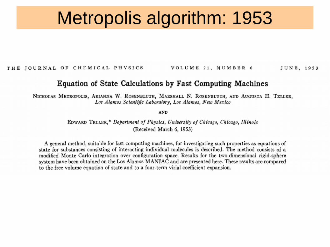
Metropolis algorithm: 1953
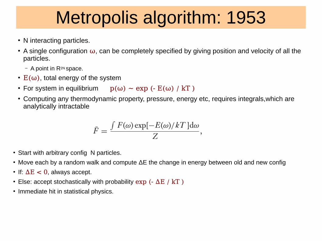
Metropolis algorithm: 1953● N interacting particles.● A single configuration ω, can be completely specified by giving position and velocity of all the
particles. – A point in R2N space.
● E(ω), total energy of the system● For system in equilibrium p(ω) ~ exp (- E(ω) / kT )● Computing any thermodynamic property, pressure, energy etc, requires integrals,which are
analytically intractable
● Start with arbitrary config N particles.● Move each by a random walk and compute ΔE the change in energy between old and new config● If: ΔE < 0, always accept.● Else: accept stochastically with probability exp (- ΔE / kT ) ● Immediate hit in statistical physics.

Hastings 1970● The same method can be used to sample an
arbitrary pdf p(ω) – by replacing E(ω)/kT → -ln p(ω)– Had to wait till Hastings
● Generalized the algorithm and derived the essential condition that a Markov chain out to satisfy to sample the target distribution.
● Acceptance ratio not uniquely specified, other forms exist.
● His student Peskun 1973 showed that Metropolis gives the fastest mixing rate of the chain

1980● Simulated annealing Kirkpatrick 1983
– To solve combinatorial optimization problems using MH algorithm using ideas of annealing from solid state physics.
● Useful when we have multiple maxima● Minimize an objective function C(ω) by sampling from exp(-C(ω)/T) with progressively decreasing T.● Allowing selection of globally optimum solution.
1984 ● Expectation Maximization (EM) algorithm
– Dempster 1977– Provided a way to deal with missing data and hidden
variables. Hierachical Bayesian models.– Vastly increased the range of problems that can addressed
by Bayesian methods.– Deterministic and sensitive to initial condition.– Stochastic versions were developed – Data augmentation, Tanner and Wong 1987
● Geman and Geman 1984– Introduced Gibbs sampling in the context of image
restoration. – First proper use of MCMC to solve a problem setup in
Bayesian framework.
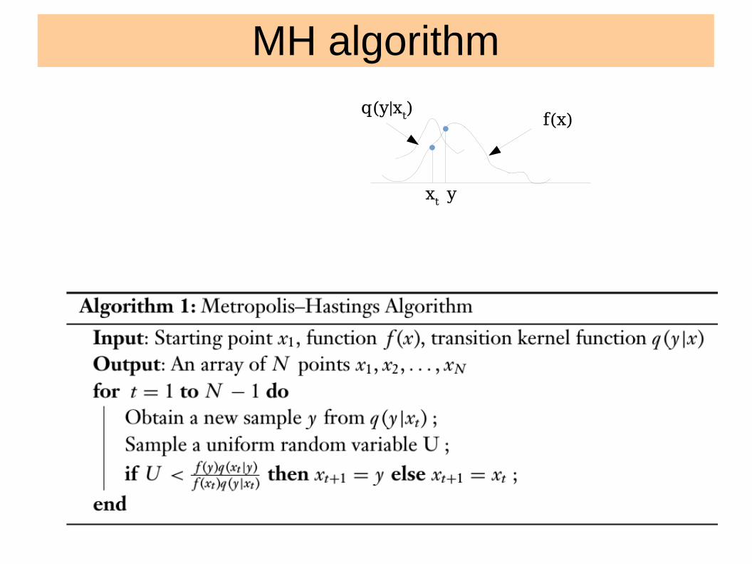
MH algorithm
f(x)q(y|xt)xt y

Image: Ryan Adams

1990● Gelfand and Smith 1990
– Largely credited with revolution in statistics,– Unified the ideas of Gibbs sampling, DA algorithm
and EM algorithm. – It firmly established that Gibbs samling and MH
based MCMC algorithms can be used to solve a wide class of problems that fall in the category of hierarchical bayesian models.
●

Citation history of Metropolis et al/ 1953
● Physics: well known from 1970-1990● Statistics: only 1990 onwards● Astronomy: 2002 onwards

Astronomy's conversion- 2002
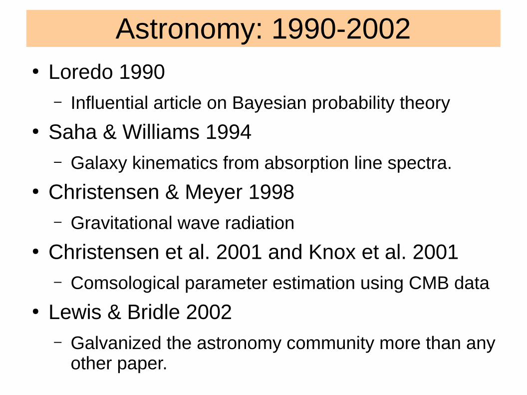
Astronomy: 1990-2002● Loredo 1990
– Influential article on Bayesian probability theory● Saha & Williams 1994
– Galaxy kinematics from absorption line spectra.● Christensen & Meyer 1998
– Gravitational wave radiation● Christensen et al. 2001 and Knox et al. 2001
– Comsological parameter estimation using CMB data● Lewis & Bridle 2002
– Galvanized the astronomy community more than any other paper.

●Lewis & Bridle 2002● Laid out in detail the Bayesian MCMC
framework● Applied it to one of the most important data sets
of the time.● Used it to address a significant scientific
question- fundamanetal parameters of the universe.
● Made the code publicly available– Making it easier for new entrants.

Present
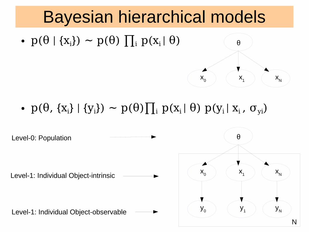
Bayesian hierarchical models● p(θ | {xi}) ~ p(θ) ∏i p(xi | θ)
● p(θ, {xi} | {yi}) ~ p(θ)∏i p(xi | θ) p(yi | xi , σyi)θ
x0
y0
N
Level-0: Population
Level-1: Individual Object-intrinsic
Level-1: Individual Object-observabley
1y
N
x1
xN
θ
x0
x1
xN

Bayesian hierarchical models● p(θ | {xi} ) ~ p(θ) ∏i p( xi | θ )
● p(θ, {xi} | {yi}) ~ p(θ) ∏i p( xi | θ ) p(yi | xi , σyi)θ
x0
y0
N
Level-0: Population
Level-1: Individual Object-intrinsic
Level-1: Individual Object-observabley
1y
N
x1
xN
θ
x0
x1
xN
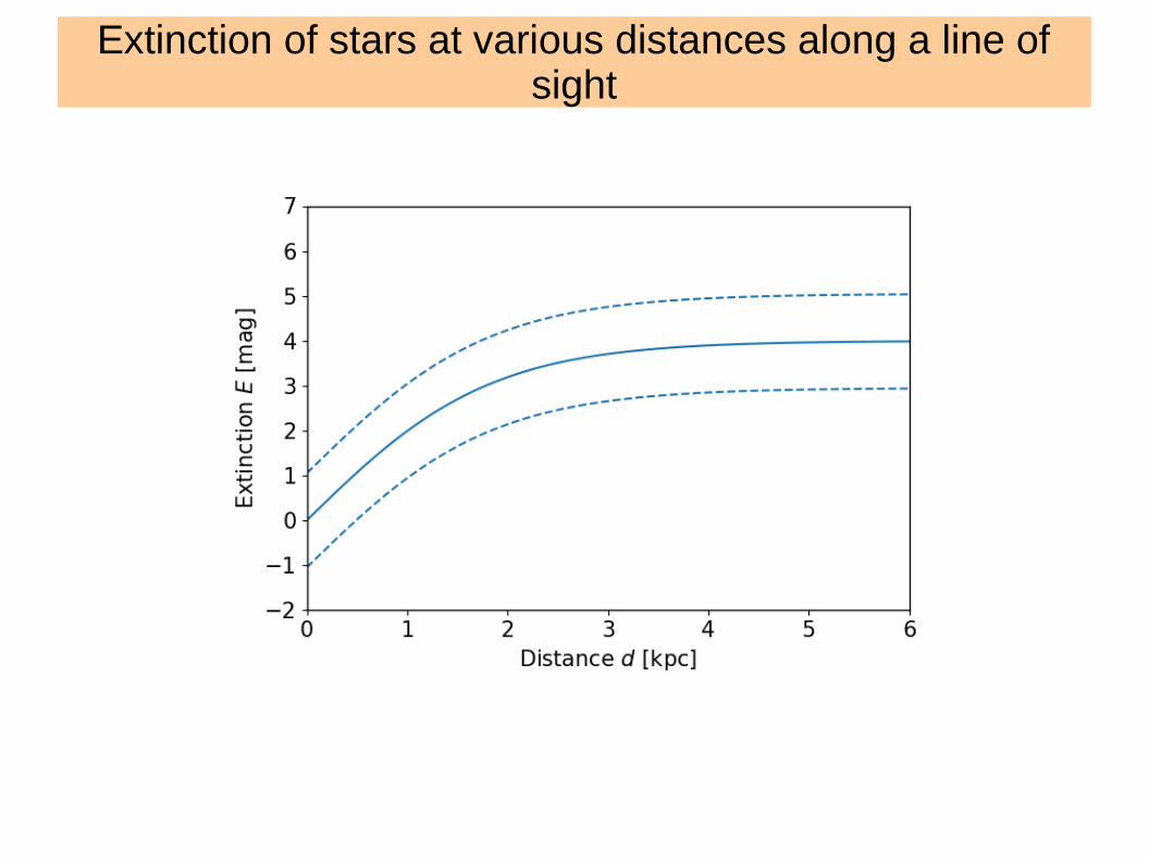
Extinction of stars at various distances along a line of sight

● What we want to know– Overall distance extinction relationship and its dispersion (α,Emax,σE).– Extinction of a star and its uncertainty p(Et,j).
● Each star has some some measurement with some uncertainty – p(Et,j|Ej) ~ Normal(Ej,σj).

BHM● Some stars have very high uncertainty. ● There is more information in data from other
stars. – p(Et,j|α,Emax,σE,Ej,σj) ~ p(Et,j|α,EmaxσE) p(Et,j | E,σj)–
● But, population statistics depends on stars, they are interrelated.
● We get joint info about population of stars as well as for individual stars. – p(α,Emax,σE, Et,j|Ej,σj) ~ p(α,Emax,σE) ∏j p(Et,j|α,EmaxσE) p(Et,j | Ej,σj)

Shrinkage of error, shift towards mean


Handling uncertainties● p(θ, {xti} | {xi}, {σxi} ) ~ p(θ) ∏i p( xti | θ ) p(xi | xti , σx,i)● p(xi | xti , σx,i) ~ Normal( xi | xti, σyi)
θxt0
x0 N
Level-0: Population
Level-1: Individual Object-intrinsic
Level-2: Individual Object-observable x1 xN
xt1 xtN
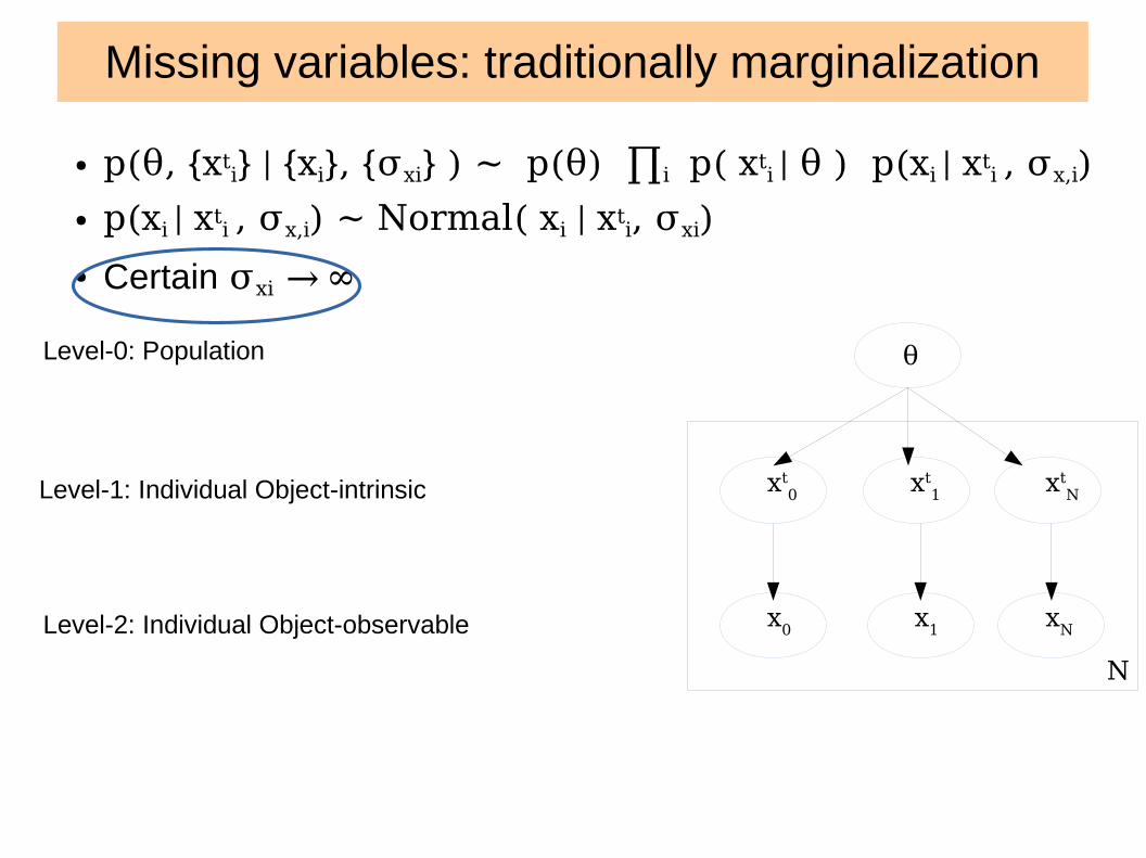
Missing variables: traditionally marginalization
● p(θ, {xti} | {xi}, {σxi} ) ~ p(θ) ∏i p( xti | θ ) p(xi | xti , σx,i)● p(xi | xti , σx,i) ~ Normal( xi | xti, σxi)● Certain σxi → ∞
θxt0
x0 N
Level-0: Population
Level-1: Individual Object-intrinsic
Level-2: Individual Object-observable x1 xN
xt1 xtN
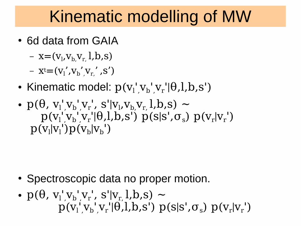
Kinematic modelling of MW● 6d data from GAIA
– x=(vl,vb,vr, l,b,s)– xt=(vl’,vb’,vr,’ ,s’)
● Kinematic model: p(vl',vb',vr'|θ,l,b,s')● p(θ, vl',vb',vr', s'|vl,vb,vr, l,b,s) ~ p(vl',vb',vr'|θ,l,b,s') p(s|s',σs) p(vr|vr') p(vl|vl')p(vb|vb')● Spectroscopic data no proper motion. ● p(θ, vl',vb',vr', s'|vr, l,b,s) ~ p(vl',vb',vr'|θ,l,b,s') p(s|s',σs) p(vr|vr')
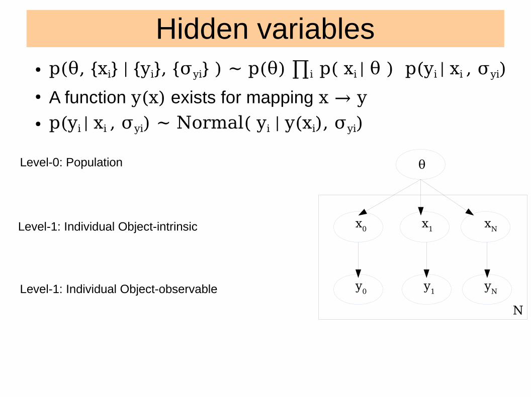
Hidden variables● p(θ, {xi} | {yi}, {σyi} ) ~ p(θ) ∏i p( xi | θ ) p(yi | xi , σyi)● A function y(x) exists for mapping x → y● p(yi | xi , σyi) ~ Normal( yi | y(xi), σyi)
θx0
y0 N
Level-0: Population
Level-1: Individual Object-intrinsic
Level-1: Individual Object-observable y1 yN
x1 xN

Intrinsic variables of a star.● Intrinsic params: x=([M/H],τ,m,s,l,b,E)● Obsevables: y=(J, H, K, Teff, log g, [M/H], l, b)● Given x one can compute y using isochrones● There exists a function y(x) mapping x to y.

Hidden variables● p(θ, {xi} | {yi}, {σyi} ) ~ p(θ) ∏i p( xi | θ ) p(yi | xi , σyi)● A function y(x) exists for mapping x → y● p(yi | xi , σyi) ~ Normal( yi | y(xi), σyi)
θx0
y0 N
Level-0: Population
Level-1: Individual Object-intrinsic
Level-1: Individual Object-observable y1 yN
x1 xN
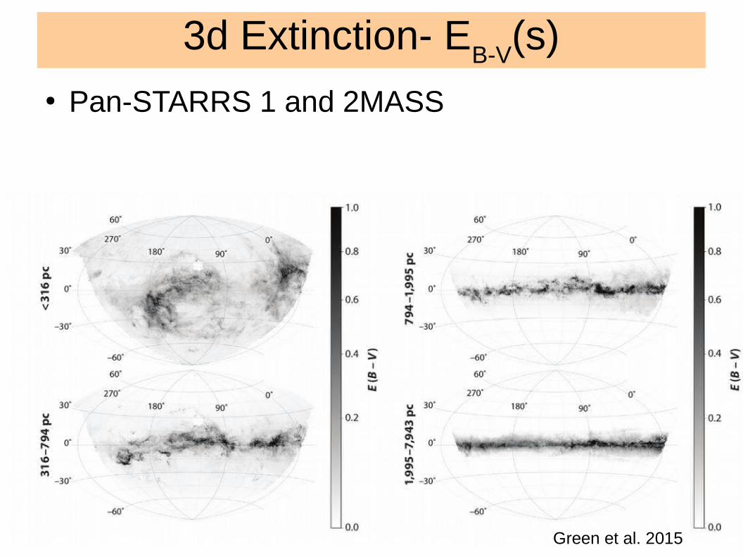
3d Extinction- EB-V
(s)● Pan-STARRS 1 and 2MASS
Green et al. 2015

Exoplanets
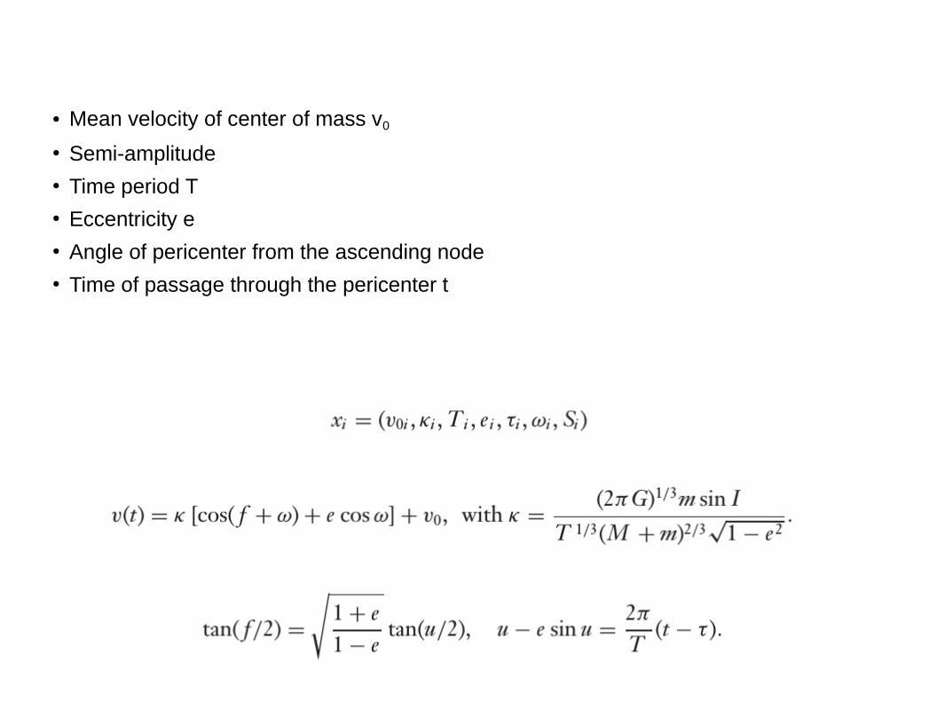
● Mean velocity of center of mass v0
● Semi-amplitude ● Time period T● Eccentricity e● Angle of pericenter from the ascending node ● Time of passage through the pericenter t


● Hogg et al 2010

● Hogg et al 2010
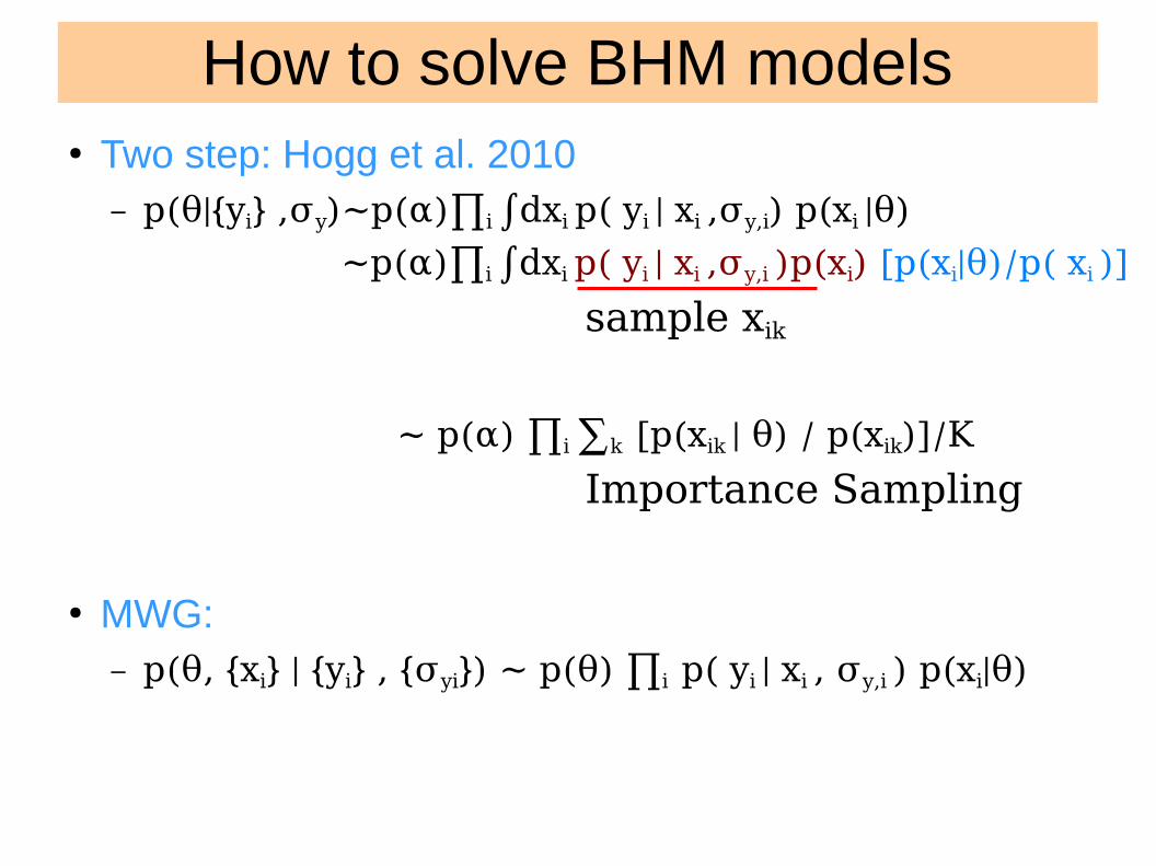
How to solve BHM models● Two step: Hogg et al. 2010
– p(θ|{yi} ,σy)~p(α)∏i ∫dxi p( yi | xi ,σy,i) p(xi |θ) ~p(α)∏i ∫dxi p( yi | xi ,σy,i )p(xi) [p(xi|θ)/p( xi )] sample xik ~ p(α) ∏i ∑k [p(xik | θ) / p(xik)]/K Importance Sampling
● MWG: – p(θ, {xi} | {yi} , {σyi}) ~ p(θ) ∏i p( yi | xi , σy,i ) p(xi|θ)

MH algorithm
f(x)q(y|x
t)
xt
y

Image: Ryan Adams

Metropolis Within Gibbs● Gibbs sampler requires sampling from
conditional distribution.● Replace this with a MH step.● Rather than updating all at one time, one can
do it one dimension at a time. ● A complicated distribution can be broken up into
sequence of smaller or easier to samplings is the main strength of this.

BMCMC- a python package● pip install bmcmc● https://github.com/sanjibs/bmcmc● Ability to solve hierarchical Bayesian models.● Documentation:
– http://bmcmc.readthedocs.io/en/latest/


Future

Future
Machine Learning Image:www.iamwire.com
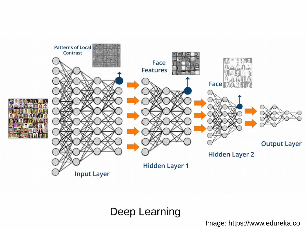
Image: https://www.edureka.co
Deep Learning
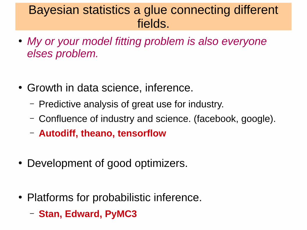
Bayesian statistics a glue connecting different fields.
● My or your model fitting problem is also everyone elses problem.
● Growth in data science, inference.– Predictive analysis of great use for industry.– Confluence of industry and science. (facebook, google).– Autodiff, theano, tensorflow
● Development of good optimizers.
● Platforms for probabilistic inference.– Stan, Edward, PyMC3

Future● Big Data
– Tall (N), Wide (dy),
– Model: Complexity (dθ), Hierarchies
● MCMC too slow
– MLE, optimization
– Speed up traditional MCMC for tall data.
– Hamiltonian Monte Carlo
– Variational Bayes
Bayesian nonparametrics (BNP)● Useful for big data.● Properties of big data
– Feature space is large → complex models– Difficult to find suitable model.

Big data analogy● More the data, more
substructures and more hierachy of substructures.
● A flexible model whose complexity can grow with data size.– Polynomials with degree
being free– Gaussian mixture model
with number of clusters free

BNP● p(x | θ) = ∑ αi Normal(x | μi, σi2), i={1,…,K}● Put a prior on p(K)● Can do this without Bayesian model comparison.● Dirichlet Process mixture models (Neal 2000).
– A prior on p(α), K → ∞

Pseudo marginal MCMC for big data● Speeding up MCMC for big data.● Subsample the data and compute the likelihood
– f’(x,y), y set of rows to use
– f’(x,y)=∑i log f(xi), for each i in y● Likelihood becomes stochastic.● Other cases of stochastic likelihood.
– Marginalization problems● p(θ|x)= ∫ p(x|θ,α)dα = ∫ ∫p(x,z|θ,α,z)dα dz
– Doubly intractable integrals
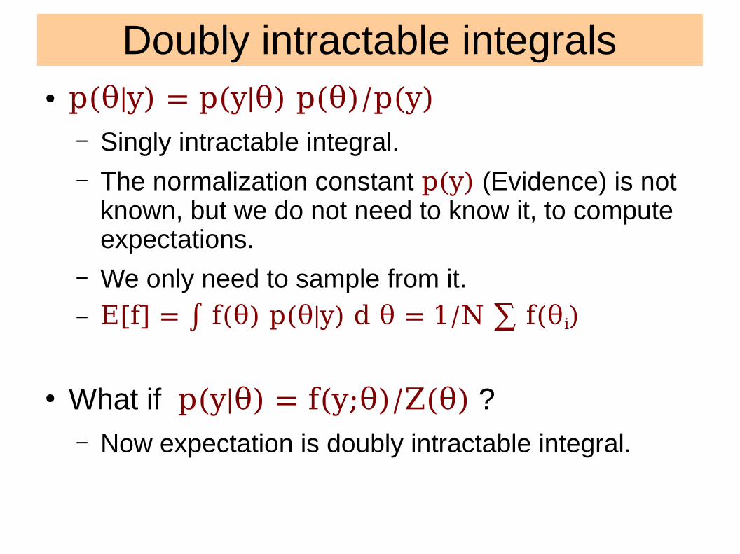
Doubly intractable integrals● p(θ|y) = p(y|θ) p(θ)/p(y)
– Singly intractable integral.– The normalization constant p(y) (Evidence) is not
known, but we do not need to know it, to compute expectations.
– We only need to sample from it. – E[f] = ∫ f(θ) p(θ|y) d θ = 1/N ∑ f(θi)
● What if p(y|θ) = f(y;θ)/Z(θ) ?
– Now expectation is doubly intractable integral.
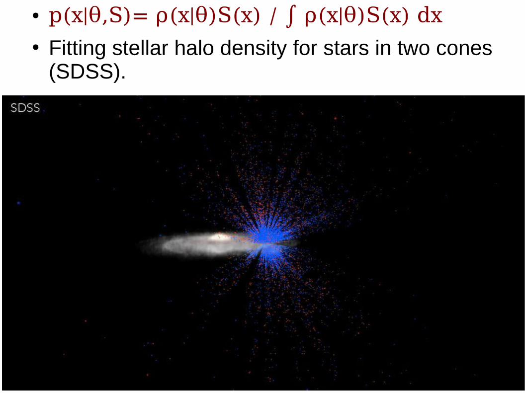
● p(x|θ,S)= ρ(x|θ)S(x) / ∫ ρ(x|θ)S(x) dx● Fitting stellar halo density for stars in two cones
(SDSS).

Handling stochastic likelihoods● Monte Carlo Metropolis-Hastings ● If U < f(x’)/f(x):
xl.append(x’)
Else:
xl.append(x)
● What if the function f is stochastic?
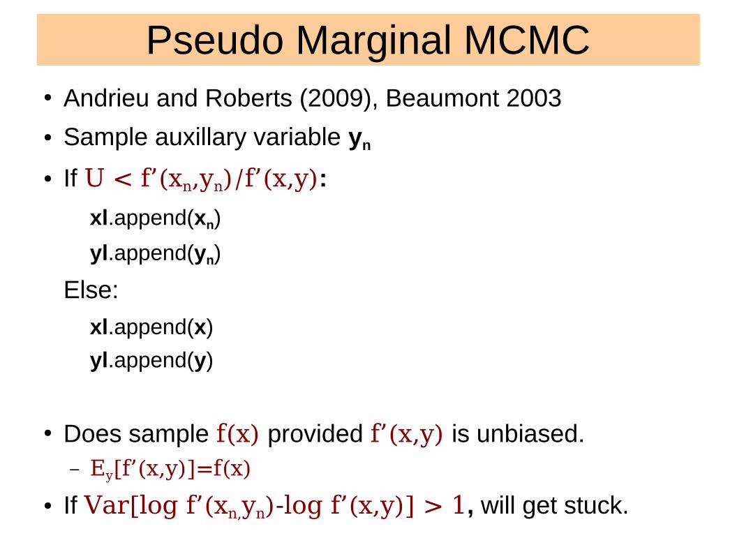
Pseudo Marginal MCMC● Andrieu and Roberts (2009), Beaumont 2003● Sample auxillary variable yn
● If U < f’(xn,yn)/f’(x,y): xl.append(xn)
yl.append(yn)
Else:
xl.append(x)
yl.append(y)
● Does sample f(x) provided f’(x,y) is unbiased.– Ey[f’(x,y)]=f(x)
● If Var[log f’(xn,yn)-log f’(x,y)] > 1, will get stuck.

Approximate MCMCMurray 2006, Liang 2011, Sharma 2014, Sharma 2017
● Sample yn
● If U < f’(xn,yn)/f’(x,yn):
xl.append(xn)
yl.append(yn)
Else:
xl.append(x)
yl.append(yn)
●
● Does not sample f(x), rather fapprox(x)● More stable, does not get stuck.

Pseudo marginal MCMC for big data● Speeding up MCMC for big data.● Subsample the data and compute the likelihood
– f’(x,y), y set of rows to use
– f’(x,y)=∑i log f(xi), for each i in y
● Unbiased for log(f(x)) but this does not give an unbiased estimator of f(x).
● Bardent 2014, Korattikara 2014, Maclaurin & Adams 2014, Quiroz (2016,2017).
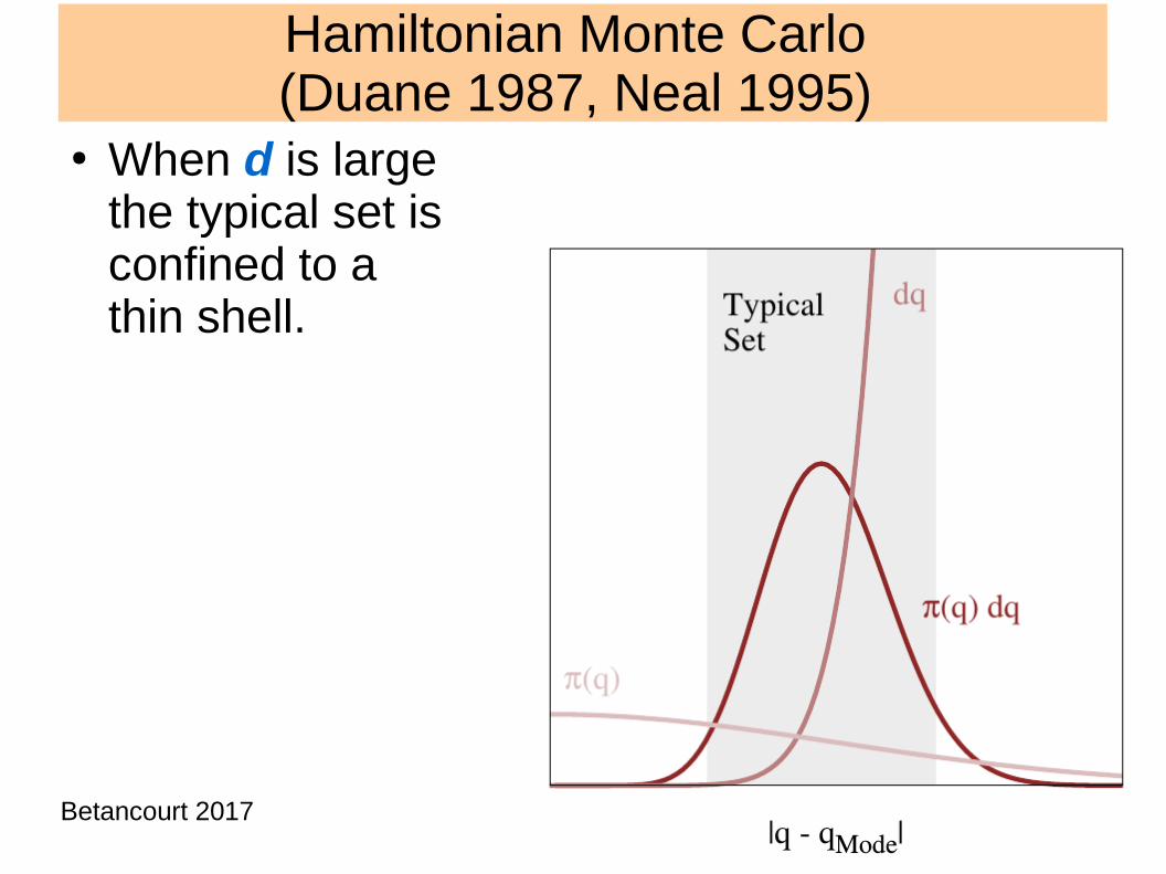
Hamiltonian Monte Carlo (Duane 1987, Neal 1995)
● When d is large the typical set is confined to a thin shell.
Betancourt 2017

Jump to unexplored areas (like punching through a wormhole). Betancourt 2017
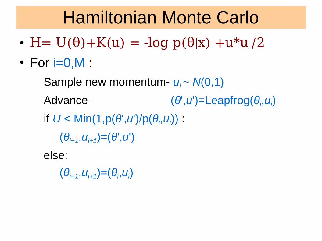
Hamiltonian Monte Carlo● H= U(θ)+K(u) = -log p(θ|x) +u*u /2● For i=0,M :
Sample new momentum- ui ~ N(0,1)
Advance- (θ',u')=Leapfrog(θi,ui)
if U < Min(1,p(θ',u')/p(θi,ui)) :
(θi+1,ui+1)=(θ',u')
else:
(θi+1,ui+1)=(θi,ui)

HMC: caveats● Need Gradients
– Magic of Automatic differentiation– Driven by rapid advances in machine learning
● Tuning of stepsize :– The No-U-Trun-Sampler (NUTS)
● Hoffman & Gelman (2014)
● Solves the high d problem.● Subsampling HMC, Dang et al. (2017), see also
Betancourt 2015 that it is difficult to do so.
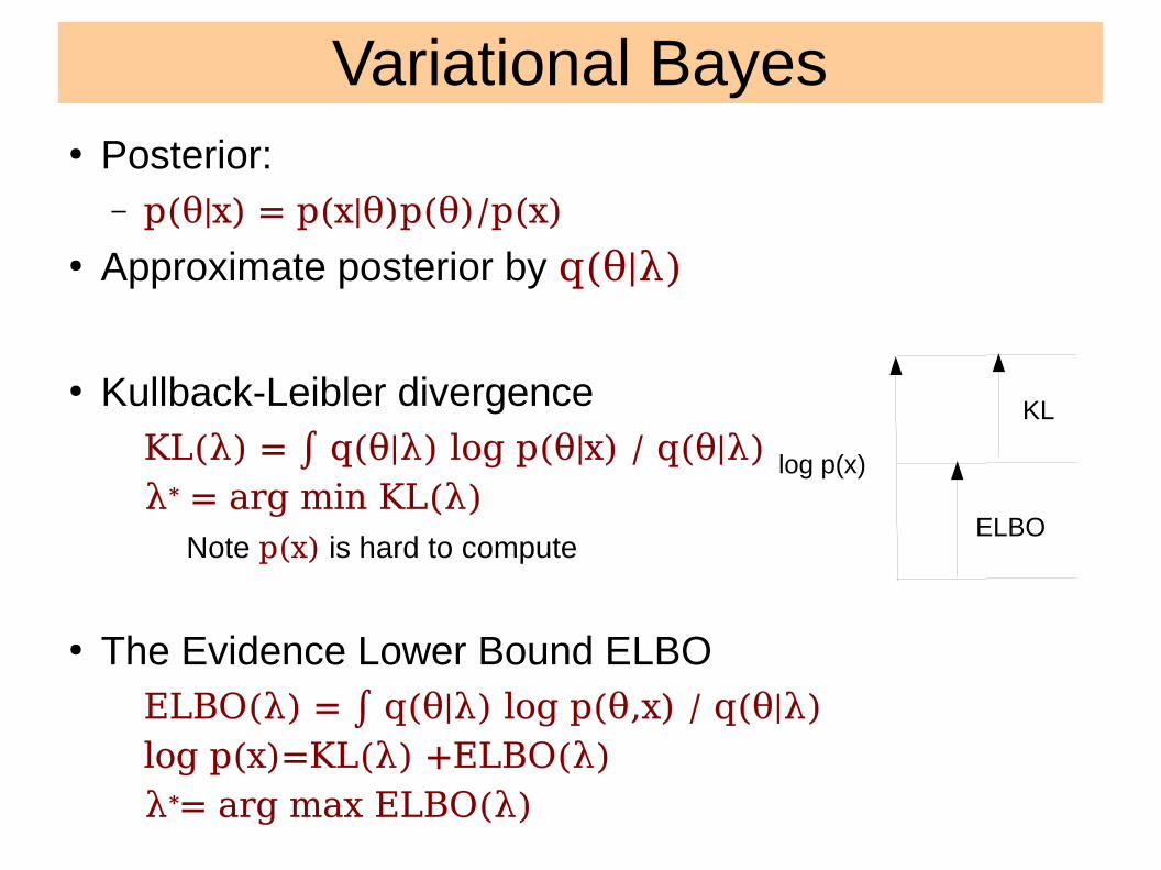
Variational Bayes● Posterior:
– p(θ|x) = p(x|θ)p(θ)/p(x)● Approximate posterior by q(θ|λ)● Kullback-Leibler divergenceKL(λ) = ∫ q(θ|λ) log p(θ|x) / q(θ|λ)λ* = arg min KL(λ)
Note p(x) is hard to compute
● The Evidence Lower Bound ELBOELBO(λ) = ∫ q(θ|λ) log p(θ,x) / q(θ|λ)log p(x)=KL(λ) +ELBO(λ)λ*= arg max ELBO(λ)
ELBO
KL
log p(x)
Variational Bayes● Reduced to an optimization problem● ADVI:
– Automatic differentiation, Variational inference– Leveraging advances in ML– Stan, Edward
● Works both for large N and d

Summary● Hierarchical Bayesian models allow you to tackle a
wide range of problems in astronomy.● Large N: Bayesian nonparametric modelling.● Large dim d -Hamiltonian Monte Carlo● Large N, large d- Variational Bayes.● For more info and Monte Carlo based algorithms to
solve Bayesian inference problems see, Sharma 2017


