Download - Basic to Reliability Process
Marvin Rausand, March 14, 2006 System Reliability Theory (2nd ed), Wiley, 2004 – 1 / 31
Chapter 2Failure Models
Part 1: Introduction
Marvin Rausand
Department of Production and Quality EngineeringNorwegian University of Science and Technology

Introduction
Introduction
Rel. measures
Life distributions
State variable
Time to failure
Distr. function
Probability density
Distribution of T
Reliability funct.
Failure rate
Bathtub curve
Some formulas
MTTF
Example 2.1
Median
Mode
MRL
Example 2.2
Discretedistributions
Life distributions
Marvin Rausand, March 14, 2006 System Reliability Theory (2nd ed), Wiley, 2004 – 2 / 31
Reliability measures
Introduction
Rel. measures
Life distributions
State variable
Time to failure
Distr. function
Probability density
Distribution of T
Reliability funct.
Failure rate
Bathtub curve
Some formulas
MTTF
Example 2.1
Median
Mode
MRL
Example 2.2
Discretedistributions
Life distributions
Marvin Rausand, March 14, 2006 System Reliability Theory (2nd ed), Wiley, 2004 – 3 / 31
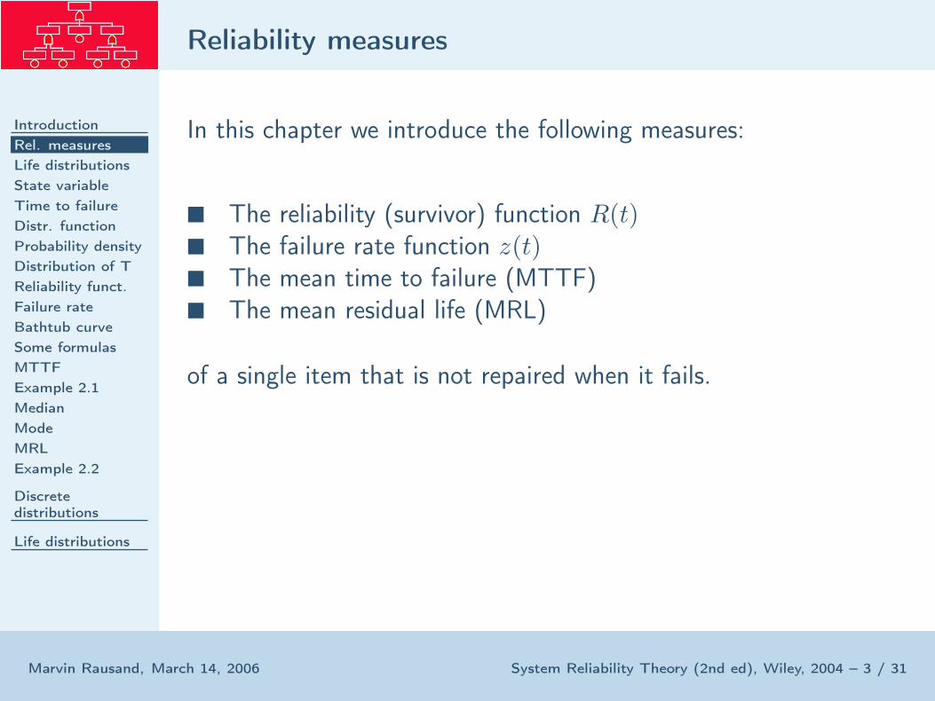
In this chapter we introduce the following measures:
■ The reliability (survivor) function R(t)■ The failure rate function z(t)■ The mean time to failure (MTTF)■ The mean residual life (MRL)
of a single item that is not repaired when it fails.

Life distributions
Introduction
Rel. measures
Life distributions
State variable
Time to failure
Distr. function
Probability density
Distribution of T
Reliability funct.
Failure rate
Bathtub curve
Some formulas
MTTF
Example 2.1
Median
Mode
MRL
Example 2.2
Discretedistributions
Life distributions
Marvin Rausand, March 14, 2006 System Reliability Theory (2nd ed), Wiley, 2004 – 4 / 31
The following life distributions are discussed:
■ The exponential distribution■ The gamma distribution■ The Weibull distribution■ The normal distribution■ The lognormal distribution■ The Birnbaum-Saunders distribution■ The inverse Gaussian distributions
In addition we cover three discrete distributions:
■ The binomial distribution■ The Poisson distribution■ The geometric distribution

State variable
Introduction
Rel. measures
Life distributions
State variable
Time to failure
Distr. function
Probability density
Distribution of T
Reliability funct.
Failure rate
Bathtub curve
Some formulas
MTTF
Example 2.1
Median
Mode
MRL
Example 2.2
Discretedistributions
Life distributions
Marvin Rausand, March 14, 2006 System Reliability Theory (2nd ed), Wiley, 2004 – 5 / 31
X(t)
0t
1
Time to failure, T
Failure
X(t) =
{
1 if the item is functioning at time t0 if the item is in a failed state at time t
The state variable X(t) and the time to failure T will generallybe random variables.

Time to failure
Introduction
Rel. measures
Life distributions
State variable
Time to failure
Distr. function
Probability density
Distribution of T
Reliability funct.
Failure rate
Bathtub curve
Some formulas
MTTF
Example 2.1
Median
Mode
MRL
Example 2.2
Discretedistributions
Life distributions
Marvin Rausand, March 14, 2006 System Reliability Theory (2nd ed), Wiley, 2004 – 6 / 31
Different time concepts may be used, like
■ Calendar time■ Operational time■ Number of kilometers driven by a car■ Number of cycles for a periodically working item■ Number of times a switch is operated■ Number of rotations of a bearing
In most applications we will assume that the time to failure T is acontinuous random variable (Discrete variables may beapproximated by a continuous variable)

Distribution function
Introduction
Rel. measures
Life distributions
State variable
Time to failure
Distr. function
Probability density
Distribution of T
Reliability funct.
Failure rate
Bathtub curve
Some formulas
MTTF
Example 2.1
Median
Mode
MRL
Example 2.2
Discretedistributions
Life distributions
Marvin Rausand, March 14, 2006 System Reliability Theory (2nd ed), Wiley, 2004 – 7 / 31
The distribution function of T is
F (t) = Pr(T ≤ t) =
∫ t
0f(u) du for t > 0
Note thatF (t) = Probability that the item will fail within the interval (0, t]

Probability density function
Introduction
Rel. measures
Life distributions
State variable
Time to failure
Distr. function
Probability density
Distribution of T
Reliability funct.
Failure rate
Bathtub curve
Some formulas
MTTF
Example 2.1
Median
Mode
MRL
Example 2.2
Discretedistributions
Life distributions
Marvin Rausand, March 14, 2006 System Reliability Theory (2nd ed), Wiley, 2004 – 8 / 31
The probability density function (pdf) of T is
f(t) =d
dtF (t) = lim
∆t→∞
F (t + ∆t) − F (t)
∆t= lim
∆t→∞
Pr(t < T ≤ t + ∆
∆t
When ∆t is small, then
Pr(t < T ≤ t + ∆t) ≈ f(t) · ∆t
0 t
∆ t
Time
When we are standing at time t = 0 and ask: What is theprobability that the item will fail in the interval (t, t + ∆t]? Theanswer is approximately f(t) · ∆t

Distribution of T
Introduction
Rel. measures
Life distributions
State variable
Time to failure
Distr. function
Probability density
Distribution of T
Reliability funct.
Failure rate
Bathtub curve
Some formulas
MTTF
Example 2.1
Median
Mode
MRL
Example 2.2
Discretedistributions
Life distributions
Marvin Rausand, March 14, 2006 System Reliability Theory (2nd ed), Wiley, 2004 – 9 / 31
■ The area under the pdf-curve (f(t)) is always 1,∫
∞
0 f(t) dt = 1■ The area under the pdf-curve to the left of t is equal to F (t)■ The area under the pdf-curve between t1 and t2 is
F (t2) − F (t1) = Pr(t1 < T ≤ t2)

Reliability Function
Introduction
Rel. measures
Life distributions
State variable
Time to failure
Distr. function
Probability density
Distribution of T
Reliability funct.
Failure rate
Bathtub curve
Some formulas
MTTF
Example 2.1
Median
Mode
MRL
Example 2.2
Discretedistributions
Life distributions
Marvin Rausand, March 14, 2006 System Reliability Theory (2nd ed), Wiley, 2004 – 10 / 31
R(t) = Pr(T > t) = 1 − F (t) =
∫
∞
tf(u) du
■ R(t) = The probability that the item will not fail in (0, t]■ R(t) = The probability that the item will survive at least to
time t■ R(t) is also called the survivor function of the item

Failure rate function
Introduction
Rel. measures
Life distributions
State variable
Time to failure
Distr. function
Probability density
Distribution of T
Reliability funct.
Failure rate
Bathtub curve
Some formulas
MTTF
Example 2.1
Median
Mode
MRL
Example 2.2
Discretedistributions
Life distributions
Marvin Rausand, March 14, 2006 System Reliability Theory (2nd ed), Wiley, 2004 – 11 / 31
Consider the conditional probability
Pr(t < T ≤ t + ∆t | T > t) =Pr(t < T ≤ t + ∆t)
Pr(T > t)
=F (t + ∆t) − F (t)
R(t)
The failure rate function of the item is
z(t) = lim∆t→0
Pr(t < T ≤ t + ∆t | T > t)
∆t
= lim∆t→0
F (t + ∆t) − F (t)
∆t·
1
R(t)=
f(t)
R(t)
When ∆t is small, we have
Pr(t < T ≤ t + ∆t | T > t) ≈ z(t) · ∆t

Failure Rate Function (2)
Introduction
Rel. measures
Life distributions
State variable
Time to failure
Distr. function
Probability density
Distribution of T
Reliability funct.
Failure rate
Bathtub curve
Some formulas
MTTF
Example 2.1
Median
Mode
MRL
Example 2.2
Discretedistributions
Life distributions
Marvin Rausand, March 14, 2006 System Reliability Theory (2nd ed), Wiley, 2004 – 12 / 31
0 t
∆ t
Time
■ Note the difference between the failure rate function z(t) andthe probability density function f(t).
■ When we follow an item from time 0 and note that it is stillfunctioning at time t, the probability that the item will failduring a short interval of length ∆t after time t is z(t) · ∆t
■ The failure rate function is a “property” of the item and issometimes called the force of mortality (FOM) of the item.

Bathtub curve
Introduction
Rel. measures
Life distributions
State variable
Time to failure
Distr. function
Probability density
Distribution of T
Reliability funct.
Failure rate
Bathtub curve
Some formulas
MTTF
Example 2.1
Median
Mode
MRL
Example 2.2
Discretedistributions
Life distributions
Marvin Rausand, March 14, 2006 System Reliability Theory (2nd ed), Wiley, 2004 – 13 / 31
z(t)
Time t0
Burn-in
period Useful life periodWear-out
period

Some formulas
Introduction
Rel. measures
Life distributions
State variable
Time to failure
Distr. function
Probability density
Distribution of T
Reliability funct.
Failure rate
Bathtub curve
Some formulas
MTTF
Example 2.1
Median
Mode
MRL
Example 2.2
Discretedistributions
Life distributions
Marvin Rausand, March 14, 2006 System Reliability Theory (2nd ed), Wiley, 2004 – 14 / 31
Expressed
by F (t) f(t) R(t) z(t)
F (t) = –
Z
t
0
f(u) du 1 − R(t) 1 − exp
„
−
Z
t
0
z(u) du
«
f(t) =d
dtF (t) – −
d
dtR(t) z(t) · exp
„
−
Z
t
0
z(u) du
«
R(t) = 1 − F (t)
Z
∞
t
f(u) du – exp
„
−
Z
t
0
z(u) du
«
z(t) =dF (t)/dt
1 − F (t)
f(t)R
∞
tf(u) du
−
d
dtlnR(t) –

Mean time to failure
Introduction
Rel. measures
Life distributions
State variable
Time to failure
Distr. function
Probability density
Distribution of T
Reliability funct.
Failure rate
Bathtub curve
Some formulas
MTTF
Example 2.1
Median
Mode
MRL
Example 2.2
Discretedistributions
Life distributions
Marvin Rausand, March 14, 2006 System Reliability Theory (2nd ed), Wiley, 2004 – 15 / 31
The mean time to failure, MTTF, of an item is
MTTF = E(T ) =
∫
∞
0tf(t) dt (1)
Since f(t) = −R′(t),
MTTF = −
∫
∞
0tR′(t) dt
By partial integration
MTTF = − [tR(t)]∞0 +
∫
∞
0R(t) dt
If MTTF < ∞, it can be shown that [tR(t)]∞0 = 0. In that case
MTTF =
∫
∞
0R(t) dt (2)
It is often easier to determine MTTF by (2) than by (1).

Example 2.1
Introduction
Rel. measures
Life distributions
State variable
Time to failure
Distr. function
Probability density
Distribution of T
Reliability funct.
Failure rate
Bathtub curve
Some formulas
MTTF
Example 2.1
Median
Mode
MRL
Example 2.2
Discretedistributions
Life distributions
Marvin Rausand, March 14, 2006 System Reliability Theory (2nd ed), Wiley, 2004 – 16 / 31
Consider an item with survivor function
R(t) =1
(0.2 t + 1)2for t ≥ 0
where the time t is measured in months. The probability densityfunction is
f(t) = −R′(t) =0.4
(0.2 t + 1)3
and the failure rate function is
z(t) =f(t)
R(t)=
0.4
0.2 t + 1
The mean time to failure is:
MTTF =
∫
∞
0R(t) dt = 5 months

Median
Introduction
Rel. measures
Life distributions
State variable
Time to failure
Distr. function
Probability density
Distribution of T
Reliability funct.
Failure rate
Bathtub curve
Some formulas
MTTF
Example 2.1
Median
Mode
MRL
Example 2.2
Discretedistributions
Life distributions
Marvin Rausand, March 14, 2006 System Reliability Theory (2nd ed), Wiley, 2004 – 17 / 31
Time t
0 5 10 15 20 25
f(t)
0,00
0,02
0,04
0,06
0,08 Mode
Median
MTTF
The median life tm is defined by
R(tm) = 0.50
The median divides the distribution in two halves. The item willfail before time tm with 50% probability, and will fail after timetm with 50% probability.
The mode of a life distribution is the most likely failure time,that is, the time tmode where the probability density function f(t)attains its maximum.:

Mode
Introduction
Rel. measures
Life distributions
State variable
Time to failure
Distr. function
Probability density
Distribution of T
Reliability funct.
Failure rate
Bathtub curve
Some formulas
MTTF
Example 2.1
Median
Mode
MRL
Example 2.2
Discretedistributions
Life distributions
Marvin Rausand, March 14, 2006 System Reliability Theory (2nd ed), Wiley, 2004 – 18 / 31
The mode of a life distribution is the most likely failure time,that is, the time tmode where the probability density function f(t)attains its maximum.:

Mean residual life
Introduction
Rel. measures
Life distributions
State variable
Time to failure
Distr. function
Probability density
Distribution of T
Reliability funct.
Failure rate
Bathtub curve
Some formulas
MTTF
Example 2.1
Median
Mode
MRL
Example 2.2
Discretedistributions
Life distributions
Marvin Rausand, March 14, 2006 System Reliability Theory (2nd ed), Wiley, 2004 – 19 / 31
Consider an item that is put into operation at time t = 0 and isstill functioning at time t. The probability that the item of age tsurvives an additional interval of length x is
R(x | t) = Pr(T > x + t | T > t) =Pr(T > x + t)
Pr(T > t)=
R(x + t)
R(t)
R(x | t) is called the conditional survivor function of the item atage t.
The mean residual (or, remaining) life, MRL(t), of the item atage t is
MRL(t) = µ(t) =
∫
∞
0R(x | t) dx =
1
R(t)
∫
∞
tR(x) dx

Example 2.2
Introduction
Rel. measures
Life distributions
State variable
Time to failure
Distr. function
Probability density
Distribution of T
Reliability funct.
Failure rate
Bathtub curve
Some formulas
MTTF
Example 2.1
Median
Mode
MRL
Example 2.2
Discretedistributions
Life distributions
Marvin Rausand, March 14, 2006 System Reliability Theory (2nd ed), Wiley, 2004 – 20 / 31
Consider an item with failure rate function z(t) = t/(t + 1). Thefailure rate function is increasing and approaches 1 when t → ∞.The corresponding survivor function is
R(t) = exp
(
−
∫ t
0
u
u + 1du
)
= (t + 1) e−t
MTTF =
∫
∞
0(t + 1) e−t dt = 2
The conditional survival function is
R(x | t) = Pr(T > x + t | T > t) =(t + x + 1) e−(t+x)
(t + 1) e−t=
t + x + 1
t + 1e
The mean residual life is
MRL(t) =
∫
∞
0R(x | t) dx = 1 +
1
t + 1
We see that MRL(t) is equal to 2 (= MTTF) when t = 0, thatMRL(t) is a decreasing function in t, and that MRL(t) → 1 whent → ∞.
Discrete distributions
Introduction
Discretedistributions
Binomial
Geometric
Poisson process
Life distributions
Marvin Rausand, March 14, 2006 System Reliability Theory (2nd ed), Wiley, 2004 – 21 / 31
Binomial distribution
Introduction
Discretedistributions
Binomial
Geometric
Poisson process
Life distributions
Marvin Rausand, March 14, 2006 System Reliability Theory (2nd ed), Wiley, 2004 – 22 / 31
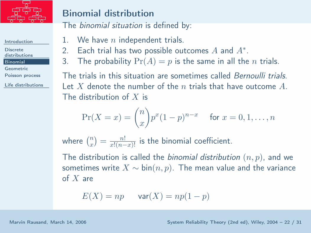
The binomial situation is defined by:
1. We have n independent trials.2. Each trial has two possible outcomes A and A∗.3. The probability Pr(A) = p is the same in all the n trials.
The trials in this situation are sometimes called Bernoulli trials.Let X denote the number of the n trials that have outcome A.The distribution of X is
Pr(X = x) =
(
n
x
)
px(1 − p)n−x for x = 0, 1, . . . , n
where(
nx
)
= n!x!(n−x)! is the binomial coefficient.
The distribution is called the binomial distribution (n, p), and wesometimes write X ∼ bin(n, p). The mean value and the varianceof X are
E(X) = np var(X) = np(1 − p)

Geometric distribution
Introduction
Discretedistributions
Binomial
Geometric
Poisson process
Life distributions
Marvin Rausand, March 14, 2006 System Reliability Theory (2nd ed), Wiley, 2004 – 23 / 31
Assume that we carry out a sequence of Bernoulli trials, and wantto find the number Z of trials until the first trial with outcome A.If Z = z, this means that the first (z− 1) trials have outcome A∗,and that the first A will occur in trial z. The distribution of Z is
Pr(Z = z) = (1 − p)z−1p for z = 1, 2, . . .
This distribution is called the geometric distribution. We havethat
Pr(Z > z) = (1 − p)z
The mean value and the variance of Z are
E(Z) =1
p
var(X) =1 − p
p2

The homogeneous Poisson process (1)
Introduction
Discretedistributions
Binomial
Geometric
Poisson process
Life distributions
Marvin Rausand, March 14, 2006 System Reliability Theory (2nd ed), Wiley, 2004 – 24 / 31
Consider occurrences of a specific event A, and assume that
1. The event A may occur at any time in the interval, and theprobability of A occurring in the interval (t, t + ∆t] isindependent of t and may be written as λ · ∆t + o(∆t),where λ is a positive constant.
2. The probability of more that one event A in the interval(t, t + ∆t] is o(∆t).
3. Let (t11, t12], (t21, t22], . . . be any sequence of disjointintervals in the time period in question. Then the events “Aoccurs in (tj1, tj2],” j = 1, 2, . . ., are independent.
Without loss of generality we let t = 0 be the starting point ofthe process.

The Homogeneous Poisson Process (2)
Introduction
Discretedistributions
Binomial
Geometric
Poisson process
Life distributions
Marvin Rausand, March 14, 2006 System Reliability Theory (2nd ed), Wiley, 2004 – 25 / 31
Let N(t) denote the number of times the event A occurs duringthe interval (0, t]. The stochastic process {N(t), t ≥ 0} is calleda Homogeneous Poisson Process (HPP) with rate λ.
The distribution of N(t) is
Pr(N(t) = n) =(λt)n
n!e−λt for n = 0, 1, 2, . . .
The mean and the variance of N(t) are
E(N(t)) =∞∑
n=0
n · Pr(N(t) = n) = λt
var(N(t)) = λt
Life distributions
Introduction
Discretedistributions
Life distributions
Exponential
Weibull
Marvin Rausand, March 14, 2006 System Reliability Theory (2nd ed), Wiley, 2004 – 26 / 31
Exponential distribution
Introduction
Discretedistributions
Life distributions
Exponential
Weibull
Marvin Rausand, March 14, 2006 System Reliability Theory (2nd ed), Wiley, 2004 – 27 / 31
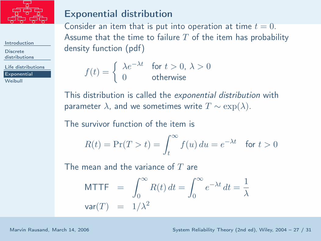
Consider an item that is put into operation at time t = 0.Assume that the time to failure T of the item has probabilitydensity function (pdf)
f(t) =
{
λe−λt for t > 0, λ > 00 otherwise
This distribution is called the exponential distribution withparameter λ, and we sometimes write T ∼ exp(λ).
The survivor function of the item is
R(t) = Pr(T > t) =
∫
∞
tf(u) du = e−λt for t > 0
The mean and the variance of T are
MTTF =
∫
∞
0R(t) dt =
∫
∞
0e−λt dt =
1
λ
var(T ) = 1/λ2

Exponential distribution (2)
Introduction
Discretedistributions
Life distributions
Exponential
Weibull
Marvin Rausand, March 14, 2006 System Reliability Theory (2nd ed), Wiley, 2004 – 28 / 31
The failure rate function is
z(t) =f(t)
R(t)=
λe−λt
e−λt= λ
The failure rate function is hence constant and independent oftime.Consider the conditional survivor function
R(x | t) = Pr(T > t + x | T > t) =Pr(T > t + x)
Pr(T > t)
=e−λ(t+x)
e−λt= e−λx = Pr(T > x) = R(x)
A new item, and a used item (that is still functioning), willtherefore have the same probability of surviving a time interval oflength t.A used item is therefore stochastically as good as new.

Weibull distribution
Introduction
Discretedistributions
Life distributions
Exponential
Weibull
Marvin Rausand, March 14, 2006 System Reliability Theory (2nd ed), Wiley, 2004 – 29 / 31
The time to failure T of an item is said to be Weibull distributedwith parameters α and λ [T ∼ Weibull(α, λ) ] if the distributionfunction is given by
F (t) = Pr(T ≤ t) =
{
1 − e−(λt)α
for t > 00 otherwise
The corresponding probability density function (pdf) is
f(t) =d
dtF (t) =
{
αλαtα−1e−(λt)α
for t > 00 otherwise
Time t
0,0 0,5 1,0 1,5 2,0 2,5 3,0
f(t)
0,0
0,5
1,0
1,5 α = 0.5
α = 1
α = 2
α = 3

Weibull distribution (2)
Introduction
Discretedistributions
Life distributions
Exponential
Weibull
Marvin Rausand, March 14, 2006 System Reliability Theory (2nd ed), Wiley, 2004 – 30 / 31
The survivor function is
R(t) = Pr(T > 0) = e−(λt)α
for t > 0
and the failure rate function is
z(t) =f(t)
R(t)= αλαtα−1 for t > 0
Time t
0,0 0,2 0,4 0,6 0,8 1,0
z(t)
0,0
0,5
1,0
1,5
2,0
α = 0.5
α = 1
α = 2α = 3

Weibull Distribution (3)
Introduction
Discretedistributions
Life distributions
Exponential
Weibull
Marvin Rausand, March 14, 2006 System Reliability Theory (2nd ed), Wiley, 2004 – 31 / 31
The mean time to failure is
MTTF =
∫
∞
0R(t) dt =
1
λΓ
(
1
α+ 1
)
The median life tm is
R(tm) = 0.50 ⇒ tm =1
λ(ln 2)1/α
The variance of T is
var(T ) =1
λ2
(
Γ
(
2
α+ 1
)
− Γ2
(
1
α+ 1
))
Note that MTTF/√
var(T ) is independent of λ.


