Download - B. Eckhardt

Turbulence transition in pipe flow:
some open questions
Bruno Eckhardt
Fachbereich Physik, Philipps-Universitat Marburg, D-35032 Marburg, Germany
Abstract. The transition to turbulence in pipe flow is a long standing problem in
fluid dynamics. In contrast to many other transitions it is not connected with linear
instabilities of the laminar profile and hence follows a different route. Experimental and
numerical studies within the last few years have revealed many unexpected connections
to the nonlinear dynamics of strange saddles and have considerably improved our
understanding of this transition. The text summarizes some of these insights and points
to a few outstanding problems in areas where nonlinear dynamics can be expected to
provide useful insights.
1. Introduction
The equations of fluid flow come naturally with a built in nonlinearity in the form of the
convective derivative and, hence, constitute a prominent playground for applications of
nonlinear dynamical systems theory. This mutually beneficial relationship has figured
prominently in bifurcation theory, the routes to chaos and the development of nonlinear
dynamics and fluid mechanics in general (see e.g. (Chandrasekhar 1961, Drazin &
Reid 1981, Koschmieder 1993). It is therefore appropriate to commemorate the 20th
anniversary of Nonlinearity by highlighting recent developments and open problems
in an area that also has a reason to celebrate an anniversary: 2008 marks the 125th
anniversary of Osborne Reynolds’s papers (Reynolds 1883a, Reynolds 1883b) on the
’Conditions which determine whether the flow of a fluid is sinuous’ in which he describes
his observations on the intermitten transition to turbulence in circular pipes. Despite
its long tradition and obvious practical relevance in many engineering situations there
are many aspects of this transition that have puzzled scientists. For instance, one
might expect that after more than a century the ’critical flow rate’, measured by
the dimensionless Reynolds number Re, for the transition to turbulence in pipe flow
should be firmly established. Instead, one finds in the literature numbers which range
between Re near 1000 (Prandtl & Tietjens 1931) and more than 3000. It turns
out that this wide range is a natural consequence of the intrinsic properties of the
system, and directly linked to the presence of a chaotic saddle. In the following,
I will summarize the work that has led to this observation as well as several other
key developements, and describe a few open questions that have come out of these

Turbulence transition in pipe flow 2
investigations. More background information as well as more details may be found in
recent reviews ((Kerswell 2005, Eckhardt, Schneider, Hof & Westerweel 2007) or the
proceedings (Mullin & (eds) 2004).
The outline is as follows. In section 2 I will summarize a few experimental and
theoretical facts about pipe flow. Section 3 then deals with coherent structures and
section 4 with their connections in state space. Section 5 discusses the issues connected
with the observed transience of turbulence. In section 6 we focus on the edge of chaos
and in section 7 on the minimal perturbations needed to trigger turbulence. The global
dynamics in relation to the localization of the turbulence in puffs is discussed in section
8. In the concluding section 9 we briefly outline connections to other shear flows.
2. Observations and elementary properties
Pressure driven flow down a smooth circular pipe develops a parabolic velocity profile
sufficiently far from the inlet. In the usual dimensionless units one measures length in
units of the diameter and velocities in units of the mean velocity. From these units
and the viscosity of the fluid one can form a dimensionless number, the Reynolds
number Re = UD/ν. Hydrodynamic similarity theory states that all flows with the
same Reynolds number, independent of flow speed or diameter of the pipe behave in
the same manner if the Reynolds numbers agree.
The unusual properties of the transition to turbulence in pipe flow are causally
connected to the fact that the parabolic profile is linearly stable agains infinitesimal
perturbations (Salwen et al. 1980, Brosa 1986, Meseguer & Trefethen 2003).
Experimentally, the laminar flow has been maintained for Reynolds numbers as high
as 100.000 (Pfenniger 1961). The non-normality of the linear operator then shows
that perturbations can temporarily extract energy from the laminar flow and give
rise to transient amplification before the final decay (Boberg & Brosa 1988, Trefethen
et al. 1993, Reddy et al. 1993, Grossmann 2000, Schmid & Henningson 1999, Waleffe
1995, Henningson 1996, Kim & Moehlis 2006, Eckhardt, Dietrich, Jachens & Schumacher
2007). This has led Meseguer and Trefethen (Meseguer & Trefethen 2003) to argue that
for Reynolds numbers in excess of 107 the transient amplification is so strong that
both experimentally and numerically it becomes practically impossible to control the
perturbations and to prevent the transition.
In view of the linear stability, the transition to turbulence requires finite amplitude
perturbations. These can derive from perturbations swept from the reservoir into the
pipe or from perturbations originating in the inflow region. A typical experiment
then shows an intermittent variation between laminar and turbulent domains which
move downstream (for experimental demonstrations on the original apparatus used by
Reynolds, see the movies provided with (Homsy et al. 2004) or (Eckhardt, Schneider, Hof
& Westerweel 2007); for time traces, see (Rotta 1956)). For controlled experiments one
turns to controlled perturbations, such as jets of fluids injected into the pipe (Wygnanski
& Champagne 1973, Wygnanski et al. 1975, Darbyshire & Mullin 1995) or devices such as

Turbulence transition in pipe flow 3
the iris diaphragm (Durst & Unsal 2006) that temporarily block the flow. For sufficiently
low Reynolds numbers these perturbations decay as they are swept downstream and do
not recover. For Reynolds numbers up to about 2400, the perturbations develop into
localized patches of about 30D lengths which move downstream with a speed close
to but not identical to the mean velocity: this implies that there is a continuous
flux of liquid through the patch. Interestingly, these patches keep their length. For
higher Reynolds number, the upstream and downstream fronts move with different
speeds and the localized patches spread out along the pipe axis. These structures
are called puffs and slugs, respectively, and are discussed extensively in (Wygnanski
& Champagne 1973, Wygnanski et al. 1975). Almost all the discussions here concern
Reynolds numbers below about 3000 and dynamics in puffs.
From a mathematical perspective, the problem is the characterization of an initial
value problem for a nonlinear, nonlocal partial differential equation, the Navier-Stokes
equation. The temporal evolution of a velocity field u(x, t) obeys
∂tu + (u · ∇)u = −∂p + ν∆u (1)
together with the incompressibility condition
∇ · u = 0 (2)
and appropriate boundary conditions. Taking the divergence of the Navier-Stokes
equation (1) gives a Poisson equation for the pressure,
∆u = −∇ · ((u · ∇)u) (3)
which results in a non-local dependence on the velocity gradients. The boundary
conditions are that the fluid velocity vanishes at the walls. In the axial direction very
often periodic boundary conditions are used. A first question, worthy of a million USD
in bounty, concerns the smoothness of solutions starting from smooth initial conditions
for all times (see (Feffermann 2000) for the prize question and (Doering & Gibbon 1995)
for some background information). Should it be possible to arrive at singularities
in finite times, then numerical representations on finite-dimensional spaces of basis
function become dubious. In the absence of any positive evidence for singularities we will
assume that the numerical representations are acceptable (modulo the usual resolution
problems).
3. Lowest Reynolds number for coherent structures
A persistent turbulent dynamics requires the presence of persistent structures in state
space other than the laminar profile. While there are examples of dynamical systems
without periodic orbits, the most likely candidates for such persistent structures are some
form of periodic motions. Perhaps the simples form are travelling waves, where a certain
velocity field flows downstream without changing its form, uTW (x, t) = u0(x − cezt) .
More complicated ones have a non-trivial time-dependence and are periodic in time
or come in the form of helical waves where a translation in time and a translation

Turbulence transition in pipe flow 4
Figure 1. Examples of coherent structures in pipe flow. The profiles are obtained
by averaging along the axis in order to highlight the symmetry. The arrows indicate
the velocity in the cross section and the color code the downstream velocity relative to
the parabolic profile. In the red regions the flow is faster than the parabola with the
same mean flux, in the blue regions it is slower. From (Faisst & Eckhardt 2003).
in downstream or azimuthal direction are coupled (so-called relative periodic states).
The method of choice for converging such states from appropriately identified initial
conditions is the Newton method, combined with various methods for obtaining good
initial conditions (see (Faisst & Eckhardt 2003, Wedin & Kerswell 2004) for pipe flow
and (Waleffe 1998, Waleffe 2001, Waleffe 2003a, Viswanath 2007b) for other flows).
For pipe flow, the structures that have first been identified are families of coherent
structures with symmetric arrangements of vortices (Faisst & Eckhardt 2003, Wedin &
Kerswell 2004) (Fig. 1). More recently, asymmetric states, still of travelling wave type,
have been identified (Pringle & Kerswell 2007). Secondary bifurcations of Hopf type will
then lead to the creation of periodic orbits, as mentioned earlier. The critical Reynolds
numbers at which the first symmetric structures appear is around 1250, that for the
asymmetric states around 770. The questions that derives from this observation is:
Question: Are there any persistent coherent states, of travelling wave or more
complicated types, with Reynolds numbers below 770?
That the lowest coherent states can be more complicated than fixed points can
be seen in studies of low-dimensional dynamical system for shear flows, where the
states that extend to the lowest Reynolds numbers are indeed periodic ones, with fixed
points appearing at much higher Reynolds numbers only (Moehlis et al. 2004, Moehlis
et al. 2005). On the other hand, this may be a resolution effect, since the low-
dimensional model is most closely related to plane Couette flow, and there the lowest
lying states are, as far as we know, again of fixed point type (Nagata 1990, Clever &
Busse 1997, Waleffe 2003b).
We do know from the study of the energy balance that for Reynolds numbers
below about 80, all perturbations decay monotonically in energy (Joseph 1975). This
then provides a lower bound. While it may be difficult to prove the existence of states,
it might be possible to prove the absence of any by establishing an asymptotic decay for
higher Reynolds numbers, following ideas from control theory (Hinrichsen et al. 2004).
The inverse question then is:
Question: What is the maximal Reynolds number below which no coherent states

Turbulence transition in pipe flow 5
can exist?
As a warmup to this problem, it might be useful to address the related question in
low-dimensional models (Eckhardt & Mersmann 1999, Moehlis et al. 2004), where the
problem is one of ordinary differential equations with quadratic nonlinearitis, and where
perhaps methods like Groebner bases can be put to good use.
4. Restructuring state space
Independent of where the first coherent states come into being at a Reynolds number of
770 or lower, it is an intriguing fact that experimental and numerical observations fail
to come up with a somewhat longer lived turbulent dynamics for Reynolds numbers
below about 1700 (Darbyshire & Mullin 1995, Peixinho & Mullin 2006, Mullin &
Peixinho 2006). Thus, while all the prerequisites for turbulence exist, the flow fails
to show turbulence in any substantial manner. This suggests:
Question: What happens in state space between the appearance of the first
coherent structures and the experimental observation of turbulence?
The problem could be a qualitative one, in that the first states that appear
are isolated and do not connect sufficiently to maintain turbulent dynamics, so that
observing turbulence requires a global bifurcation which then links different structures
to form a noticable attractor. The problem could also be simply a quantitative one, in
that the structures form soon after the first bifurcations, and in a localized region in
state space, and then simply grow and spread in until they are sufficiently volume filling
to be noticable. Most likely, the answer to the problems involves a combination of both.
Some progress towards tracking the manifolds is described in (Gibson et al. 2007).
An aspect of the restructuring is the observation that all states found so far are
unstable, which means that they cannot be observed as permanent structures. However,
it is possible to observe these states transiently in the experiment and numerics (Hof
et al. 2004, Schneider, Eckhardt & Vollmer 2007, Kerswell & Tutty 2007, Eckhardt
et al. 2005). The theory of chaotic systems holds that the frequency with which these
states appears is related to their instability (Cvitanovic & Eckhardt 1991, Eckhardt &
Ott 1994).
Question: Can the frequency with which travelling waves appear be related to
their stability?
The studies (Schneider, Eckhardt & Vollmer 2007, Kerswell & Tutty 2007) are a
first step in this direction, but cannot establish the quantitative relations between the
indicator and the stability of the identified objects.
5. Transient turbulence
Very often, turbulent dynamics is associated with the formation of an attractor: then
the dynamics would be persistent, chaotic, with an invariant measure and many other
nice features. Long ago, (Brosa 1989) noticed that all his numerical runs returned to the
Turbulence transition in pipe flow 6
t
E3D
0 250 500 750
0.01
0.02
0.03
500 1000 1500 2000t
1.0
P(t
)
15001900200020502100215021752200202517002125
Re
1000/τ
1600 2000
0
200
400
Re
1000/τ
2200200018001600
100
10
1
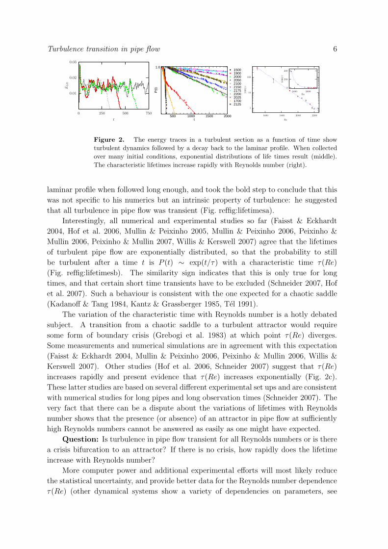
Figure 2. The energy traces in a turbulent section as a function of time show
turbulent dynamics followed by a decay back to the laminar profile. When collected
over many initial conditions, exponential distributions of life times result (middle).
The characteristic lifetimes increase rapidly with Reynolds number (right).
laminar profile when followed long enough, and took the bold step to conclude that this
was not specific to his numerics but an intrinsic property of turbulence: he suggested
that all turbulence in pipe flow was transient (Fig. reffig:lifetimesa).
Interestingly, all numerical and experimental studies so far (Faisst & Eckhardt
2004, Hof et al. 2006, Mullin & Peixinho 2005, Mullin & Peixinho 2006, Peixinho &
Mullin 2006, Peixinho & Mullin 2007, Willis & Kerswell 2007) agree that the lifetimes
of turbulent pipe flow are exponentially distributed, so that the probability to still
be turbulent after a time t is P (t) ∼ exp(t/τ) with a characteristic time τ(Re)
(Fig. reffig:lifetimesb). The similarity sign indicates that this is only true for long
times, and that certain short time transients have to be excluded (Schneider 2007, Hof
et al. 2007). Such a behaviour is consistent with the one expected for a chaotic saddle
(Kadanoff & Tang 1984, Kantz & Grassberger 1985, Tel 1991).
The variation of the characteristic time with Reynolds number is a hotly debated
subject. A transition from a chaotic saddle to a turbulent attractor would require
some form of boundary crisis (Grebogi et al. 1983) at which point τ(Re) diverges.
Some measurements and numerical simulations are in agreement with this expectation
(Faisst & Eckhardt 2004, Mullin & Peixinho 2006, Peixinho & Mullin 2006, Willis &
Kerswell 2007). Other studies (Hof et al. 2006, Schneider 2007) suggest that τ(Re)
increases rapidly and present evidence that τ(Re) increases exponentially (Fig. 2c).
These latter studies are based on several different experimental set ups and are consistent
with numerical studies for long pipes and long observation times (Schneider 2007). The
very fact that there can be a dispute about the variations of lifetimes with Reynolds
number shows that the presence (or absence) of an attractor in pipe flow at sufficiently
high Reynolds numbers cannot be answered as easily as one might have expected.
Question: Is turbulence in pipe flow transient for all Reynolds numbers or is there
a crisis bifurcation to an attractor? If there is no crisis, how rapidly does the lifetime
increase with Reynolds number?
More computer power and additional experimental efforts will most likely reduce
the statistical uncertainty, and provide better data for the Reynolds number dependence
τ(Re) (other dynamical systems show a variety of dependencies on parameters, see

Turbulence transition in pipe flow 7
e.g. (Kaneda 1990, Crutchfield & Kaneko 1988, Lai & Winslow 1995, Braun &
Feudel 1996, Goren et al. 1998, Rempel & Chian 2003)
It would also be helpful to find other indicators in the boundary dynamics, in the
fluctuations or any other quantity directly accessible from the turbulent dynamics that
might point to the existence or absence of a bifurcation. However, a definite answer
to the appearence of an attractor requires constructive criteria for the identification of
the necessary global bifurcation. But even then the turbulence need not be persistent,
as spontaneous, noise-induced transitions between the two coexisting attractors could
cause a relaminarization (Lagha & Manneville 2007, Schoepe 2004).
6. Edge of chaos
In the case of two coexisting attractors, there are basins and boundaries which separate
the basins. If the turbulence is only transient, the turbulent dynamics connects to the
laminar one, and there can be no basin boundary dividing state space into a turbulent
and a laminar region. Hence, the concept of the dividing surface between the two
regions has to be reconsidered and suitably generalized (Skufca et al. 2006, Schneider
& Eckhardt 2006, Schneider, Eckhardt & Yorke 2007, Vollmer et al. 2007)) Starting
from the properties of the saddle state in a saddle-node bifurcation, one could use the
lifetimes of perturbations, i.e. the time it takes to relax to the laminar profile, as an
indicator: approaching the stable manifold from the laminar side of the saddle, the
lifetime increases, reaches infinity and stays there, if the state on the other side is
attracting. If the state on the other side is transient, there will be wild variations in
lifteimes from one initial condition to a nearby one. Therefore, we denoted this point the
edge of chaos. All edge points seem to be connected in state space. A second observation
concerns these connections and the dynamics in the edge of chaos: numerical studies
show an evolution towards a relative attractor (see (Skufca et al. 2006) for a model
study, (Schneider & Eckhardt 2006, Schneider, Eckhardt & Vollmer 2007) for pipe flow
and (Itano & Toh 2000, Toh & Itano 2003, Viswanath 2007a) for other flows). We have
used a two-dimensional map to characterize some of these properties, including possible
bifurcations in the edge state and the appearance of chaos (Vollmer et al. 2007). Most
intriguingly, there is a possibility that this boundary can be fractal or not, depending
on the ratio of two Lyapunov exponents.
Question: What are the properties of the edge of chaos and the invariant state
within the edge? Is the edge of chaos a global relative attractor or are there additional
attractors in the edge of chaos?
The models in (Vollmer et al. 2007) can easily be extended to cover multiple
attractors in the edge, as in the model studied in (Skufca et al. 2006), but it would
be nice to have an example in a realistic flow.

Turbulence transition in pipe flow 8
7. Minimal perturbations
In cases in which the laminar profile is stable, a finite perturbation is require to
trigger turbulence. Experiments and the observations on non-normal amplification of
perturbations show that the flow becomes increasingly sensitive to perturbations as
the Reynolds number increases (Hof et al. 2003). This suggests that the diameter
of the basin of attraction of the laminar profile decreases with increasing Reynolds
number. While there are results that suggest that the boundary contracts like 1/Re
((Hof et al. 2003) and, for low Re, Fig. 3), some experiments and numerics find
steeper decays (Mellibovsky & Meseguer 2005, Mellibovsky & Meseguer 2007, Peixinho
& Mullin 2007, Philip et al. 2007).
Question: How does the amplitude of the minimal perturbation required to trigger
turbulence decay with Reynolds number?
To approach this question, one may look for minimal variations in the laminar
profile which turn it unstable (Gavarini et al. 2004), or for optimal 3-d perturbations
which triggering turbulence: (Ben-Dov & Cohen 2007) find a global minimum in energy
norm for triggering secondary instabilites. It is also possible to study the scaling
of the invariant state in the edge or perhaps of other relevant coherent states with
Reynolds number. This is facilitated by the observation that the states do not become
more complex with Re (Wang et al. 2007, Schneider 2007). In simple models they
can dominate the size of the basins (Eckhardt & Lathrop 2006), but here there is
evidence that they maintain a finite distance from the laminar profile as Re → ∞
(Wang et al. 2007):
Question: Can one characterize the Re → ∞ limit of coherent structures? Do
the solutions approach the laminar profile or do some of them keep a finite distance for
large Re?
If the states keep a finite distance from the laminar profile then the reduction in
the basin of attraction of the laminar profile has to come from a scaling of the stable
manifolds. Such an connection would also fit with the observations of kinks and folds
in the edge (Fig. 3), which are typical for stable manifolds.
8. Turbulent spot dynamics
The coherent structures described earlier provide a conveninent means for describing
the dynamics in a finite section of the pipe with periodic boundary conditions. This,
however, covers only one aspect of the dynamics, in that the experimentally induced
turbulence is usually a localized one, confined to a domain of about 30D length
(Wygnanski & Champagne 1973, Wygnanski et al. 1975) (see Fig. 4). If a shorter
turbulent region is induced, it grows until it reaches this length, if a longer one is
induced it either shrinks or breaks up into two shorter ones which again grow to be 30D
long. Therefore, there is considerable robustness in the turbulent dynamics of spots:

Turbulence transition in pipe flow 9
Re
102
A0
3840 3860 3880 3900
3.8
3.9
4.0
Re
Re
Ac
400030002000
200
100
0
2000 2250 2500
170
175
180
3000 3500 4000
145
150
155
Figure 3. The boundary between laminar and turbulent (left) for a specific
perturbation and the scaling of the boundary with Reynolds number. The insets on
the right show modulations in the scaling curve connected with the folds on the left.
From (Schneider, Eckhardt & Yorke 2007).
Figure 4. Three snapshots of a turbulent flow in a pipe at Re = 1825, moving from
left to right. The snapshots are separated in time by 20D/ucl with ucl the centerline
velocity. The red and blue regions indicate isosurfaces of downstream velocities
somewhat faster or slower than the parabolic laminar profile. The aspect ratio is
not shown to scale: the pipe is 50 diameters long. From (Eckhardt & Schneider 2008).
Question: For Reynolds numbers below about 2700, the turbulence in a long pipe
comes in localized puffs. How is the dynamics of the puffs, their length selection and
their boundary dynamics connected to the periodic coherent structures?
In the simplest form one can imagine some sort of Ginzburg-Landau type model
for the dynamics of an envelope of the turbulent region (as in (Prigent et al. 2002)), but
this is unsatisfactory unless the equations and their coefficient can be derived from the
underlying Navier-Stokes dynamics. It is interesting to note that a simliar localization
phenomenon can be studied in plane Couette flow (Barkley & Tuckerman 2005).

Turbulence transition in pipe flow 10
9. Final remarks
The discussion in the preceeding section has focussed on pipe flow, but there are
several other related problems. One is plane Couette flow between parallel plates in
relative motion, where the laminar profile is also linearly stable for all Reynolds numbers
(Dauchot & Daviaud 1994, Dauchot & Daviaud 1995, Bottin et al. 1998, Dauchot &
Vioujard 2000). Pressure driven flow between parallel plates, plane Poiseuille flow, has
a parabolic profile and a curious linear instability at Reynolds numbers of about 5772.
However, turbulence is observed at Reynolds numbers of about 1000, and hence can
follow a similar mechanism to the case described here. Finally, there is also a regime in
flow between rotating concentric cylinders, Taylor-Couette flow, where a stable laminar
profile and a turbulent dynamics coexist (Faisst & Eckhardt 2000, Hristova et al. 2002).
At present there seem to be many similiarities and connections between these flows,
suggesting that the transition to turbulence in these flows follows an independent route
with many as yet unexplored dynamical properties.
The ultimate challenge is to understand the full hydrodynamic flow and hence
the properties of the Navier-Stokes equation. But it is good to know that for the
development and test of ideas there are models on all levels of complexity, from ordinary
differential equations with varying numbers of degrees of freedom to simplified partial
differential equations, see e.g. (Waleffe 1995, Eckhardt & Mersmann 1999, Moehlis
et al. 2004, Moehlis et al. 2005, Brosa & Grossmann 1999, Smith et al. 2005, Manneville
& Locher 2000, Lagha & Manneville 2007).
Osborne Reynolds motivated his study not only with the obvious practical relevance
of pipe flow, but also with his interest in the nature of the transition. He could not
have anticipated that while he was among the first to describe a transition in detail,
his example would be among the last among to be explained. But in hindsight it is
clear that any serious explanation of the transition requires quite a bit of nonlinear
dynamics. Fortunately, the transition in pipe flow is not only at the receiving end: the
complexity of the edge state and the intriguing possibilites for the connections between
the different states in the high-dimensional state space can be expected to stimulate
nonlinear dynamics as well.
Acknowledgements
It is a pleasure to thank Holger Faisst and Tobias M. Schneider for their untiring efforts
and original contributions to elucidating the properties of transitional pipe flow, and to
Jerry Westerweel and Bjorn Hof for sharing their experiments and many ideas. This
work was supported by Deutsche Forschungsgemeinschaft.
References
Barkley D & Tuckerman L S 2005 Phys. Rev. Lett. 94, 014502.
Ben-Dov G & Cohen J 2007 Physical Review Letters 98(6), 064503–+.

Turbulence transition in pipe flow 11
Boberg L & Brosa U 1988 Z. Naturforsch. 43a, 697–726.
Bottin S, Daviaud F, Manneville P & Dauchot O 1998 Europhys. Lett. 43(2), 171–176.
Braun R & Feudel F 1996 Phys. Rev. E 53, 6562–6565.
Brosa U 1986 Zeitschrift fur Naturforschung 41a, 1141.
Brosa U 1989 J. Stat. Phys. 55, 1303–1312.
Brosa U & Grossmann S 1999 Eur. Phys. J. B 9, 343–354.
Chandrasekhar S 1961 Hydrodynamic and hydromagnetic stability Oxford University Press Oxford.
Clever R & Busse F H 1997 Journal of Fluid Mechanics 344, 137–153.
Crutchfield J P & Kaneko K 1988 Phys. Rev. Lett. 60, 2715–2718.
Cvitanovic P & Eckhardt B 1991 Journal of Physics A: Mathematical and General 24, L237–L241.
Darbyshire A G & Mullin T 1995 J. Fluid Mech. 289, 83–114.
Dauchot O & Daviaud F 1994 Europhys. Lett. 28, 225–230.
Dauchot O & Daviaud F 1995 Phys. Fluids 7, 335–343.
Dauchot O & Vioujard N 2000 Eur. Phys. J. B 14, 377.
Doering C R & Gibbon J 1995 Applied analysis of the Navier-Stokes equation Cambridge University
Press Cambridge.
Drazin P G & Reid W H 1981 Hydrodynamic Stability Cambridge University Press Cambridge.
Durst F & Unsal B 2006 Journal of Fluid Mechanics 560, 449–464.
Eckhardt B, Dietrich A, Jachens A & Schumacher J 2007 in J Peinke, ed., ‘Progress in Turbulence II’
Springer.
Eckhardt B, Faisst H, Schmiegel A & Schneider T M 2005 Phil. Trans. R Soc (London) p. submitted.
Eckhardt B & Lathrop D P 2006 Nonlinear Phenomena and Complex Systems 9, 133–140.
Eckhardt B & Mersmann A 1999 Physical Review E 60, 509–517.
Eckhardt B & Ott G 1994 Zeitschrift fur Physik B 93, 259–266.
Eckhardt B & Schneider T M 2008 European Physical Journal B p. in press.
Eckhardt B, Schneider T M, Hof B & Westerweel J 2007 Annual Review of Fluid Mechanics 39, 447–468.
Faisst H & Eckhardt B 2000 Physical Review E 61, 7227–7230.
Faisst H & Eckhardt B 2003 Physical Review Letters 91, 224502 (4 pages).
Faisst H & Eckhardt B 2004 Journal of Fluid Mechanics 504, 343–352.
Feffermann C L 2000 Existence and smoothness of the Navier-Stokes equation Technical report
http://www.claymath.org/millennium/Navier-Stokes Equations/navierstokes.pdf.
Gavarini M I, Bottaro A & Nieuwstadt F T M 2004 Journal of Fluid Mechanics 517, 131–165.
Gibson J F, Halcrow J & Cvitanovic P 2007 arxiv 0705.3957, (31 pages).
Goren G, Eckmann J P & Procaccia I 1998 Phys. Rev. E 57, 4106–4134.
Grebogi C, Ott E & Yorke J A 1983 Physica D 7, 181–200.
Grossmann S 2000 Rev. Mod. Phys. 72, 603–618.
Henningson D 1996 Physics of Fluids 8, 2257–2258.
Hinrichsen D, Plischke E & Wirth F 2004 in V. D Blondel & A Megretski, eds, ‘Unsolved problems in
mathematical systems theory’ V D Blondel and A Megretski (eds), Princeton University Press
pp. 197–202.
Hof B, Juel A & Mullin T 2003 Phys. Rev. Lett. p. 244502.
Hof B, van Doorne C W H, Westerveel J, Nieuwstadt F T M, Faisst H, Eckhardt B, Wedin H, Kerswell
R R & Waleffe F 2004 Science 305, 1594–1598.
Hof B, Westerweel J, Schneider T & Eckhardt B 2007 arxiv p. 0707.2642 (1 page).
Hof B, Westerweel J, Schneider T M & Eckhardt B 2006 Nature 443, 60–64.
Homsy G M, Aref H, Breuer G S & et al. 2004 Multi Media Fluid Mechanics Cambridge University
Press Cambridge.
Hristova H, Roch S, Schmid P J & Tuckerman L S 2002 Physics of Fluids 14, 3475–3484.
Itano T & Toh S 2000 Journal Physical Society of Japan ???, ???
Joseph D D 1975 Stability of Fluid Motions, vol I and II Springer.
Kadanoff L P & Tang C 1984 Proc. Natl. Acad. Sci. USA 81, 1276.

Turbulence transition in pipe flow 12
Kaneda K 1990 Phys. Lett. A 149, 105–112.
Kantz H & Grassberger P 1985 Physica D 17, 75–86.
Kerswell R R 2005 Nonlinearity 18, R17–R44.
Kerswell R R & Tutty O R 2007 Journal of Fluid Mechanics 584, 69–102.
Kim L & Moehlis J 2006 Physics Letters A 358, 431–437.
Koschmieder E L 1993 Benard Cells and Taylor Vortices Cambridge University Press.
Lagha M & Manneville P 2007 European Physical Journal B 58, 433–447.
Lai Y C & Winslow R L 1995 Phys. Rev. Lett. 74, 5208–5211.
Manneville P & Locher F 2000 Comptes Rendus de l’Academie des Sciences Series IIB Mechanics
Physics Astronomy 328, 159–164.
Mellibovsky F & Meseguer A 2005 Journal of Physics Conference Series 14, 192–205.
Mellibovsky F & Meseguer A 2007 Physics of Fluids ???, submitted.
Meseguer A & Trefethen L 2003 Journal of Computational Physics 186, 178–197.
Moehlis J, Faisst H & Eckhardt B 2004 New Journal of Physics 6, nr. 56 (17 pages).
Moehlis J, Faisst H & Eckhardt B 2005 SIAM Journal of Applied Dynamical Systems 4, 352–376.
Mullin T & (eds) R K 2004 Laminar-turbulent transition and finite amplitude solutions Springer
Dordrecht.
Mullin T & Peixinho J 2005 in Mullin & ???, eds, ‘IUTAM Symposium transition in shear flows’
Springer.
Mullin T & Peixinho J 2006 Journal of Low Temperature Physics 145, 75–88.
Nagata M 1990 Journal of Fluid Mechanics 217, 519–527.
Peixinho J & Mullin T 2006 Physical Review Letters 96, 094501 (4 pages).
Peixinho J & Mullin T 2007 Journal of Fluid Mechanics 582, 169–178.
Pfenniger W 1961 in G Lachman, ed., ‘Boundary Layer and Flow Control’ Pergamon pp. 970–980.
Philip J, Svizher A & Cohen J 2007 Physical Review Letters 98(15), 154502–+.
Prandtl L & Tietjens O 1931 Hydro- und Aeromechanik Julius Springer Berlin.
Prigent A, Gregoire G, Chate H, Dauchot O & van Saarloos W 2002 Phys. Rev. Lett. 89, 014501.
Pringle C & Kerswell R R 2007 Physical Review Letters 99, 074502.
Reddy S C, Schmid P J & Henningson D S 1993 SIAM Journal of Applied Mathematics 53, 15–47.
Rempel E L & Chian A C L 2003 Phys. Lett. A 319, 104–109.
Reynolds O 1883a Philosophical Transactions Royal Society (London) 174, 935–982 + 3 plates.
Reynolds O 1883b Proceedings Royal Society (London) 35, 84–99.
Rotta J 1956 Ingenieur-Archiv 24, 258–281.
Salwen H, Cotton F W & Grosch C E 1980 J. Fluid Mech. 98, 273–284.
Schmid P J & Henningson D S 1999 Stability and Transition of Shear Flows Springer New York.
Schneider T M 2007 State space properties of transitional pipe flow PhD thesis Philipps Universitat
Marburg.
Schneider T M & Eckhardt B 2006 Chaos 16, 020604.
Schneider T M, Eckhardt B & Vollmer J 2007 Physical Review E 75, 066313.
Schneider T M, Eckhardt B & Yorke J A 2007 Physical Review Letters 99, 034502.
Schoepe W 2004 Phys. Rev. Lett. 92, 095301.
Skufca J D, Yorke J A & Eckhardt B 2006 Physical Review Letters 96, 174101 (4 pages).
Smith T R, Moehlis J & Holmes P 2005 Journal of Fluid Mechanics 538, 71–110.
Tel T 1991 in H Bai-Lin, D Feng & J Yuan, eds, ‘Directions in Chaos’ Vol. 3 World Scientific, Singapore
p. 149.
Toh S & Itano T 2003 Journal of Fluid Mechanics 481, 67–76.
Trefethen L N, Trefethen A E, Reddy S C & Driscoll T A 1993 Science 261, 578–584.
Viswanath D 2007a arxiv 0701337, 15 pages.
Viswanath D 2007b Journal of Fluid Mechanics 580, 339–358.
Vollmer J, Schneider T & Eckhardt B 2007 Nonlinearity to be submitted.
Waleffe F 1995 Phys. Fluids 7, 3060–3066.

Turbulence transition in pipe flow 13
Waleffe F 1998 Physical Review Letters 81, 4140–4143.
Waleffe F 2001 Journal of Fluid Mechanics 435, 93–102.
Waleffe F 2003a Phys. Fluids 15, 1517–1534.
Waleffe F 2003b Physics of Fluids 15, 1517–1534.
Wang J, Gibson J & Waleffe F 2007 Physical Review Letters 98, 204501.
Wedin H & Kerswell R R 2004 Journal of Fluid Mechanics 508, 333–371.
Willis A P & Kerswell R R 2007 Physical Review Letters 98, 014501.
Wygnanski I J & Champagne F H 1973 Journal of Fluid Mechanics 59, 281–335.
Wygnanski I, Sokolov M & Friedman D 1975 Journal of Fluid Mechanics 69, 283–304.


