DUDLEY KNOX L^rcAKY
NAVAL POSTGKAUbA I E SCHUUU
MWTEREY.CA 93943-5101


NAVAL POSTGRADUATE SCHOOLMonterey, California
THESIS
AVIONICS SYSTEM DEVELOPMENTFOR A ROTARY WING
UNMANNED AERIAL VEHICLE
by
Daniel S. Greer
June 1998
Thesis Advisor: Russ W. Duren
Approved for public release; distribution is unlimited.


REPORT DOCUMENTATION PAGE Form ApprovedOMBNo. 0704-0188
Public reporting burden for this collection of information is estimated to average 1 hour per response, including the time for reviewing instruction,
searching existing data sources, gathering and maintaining the data needed, and completing and reviewing the collection of information. Send
comments regarding this burden estimate or any other aspect of this collection of information, including suggestions for reducing this burden, to
Washington headquarters Services, Directorate for Information Operations and Reports, 1 21 5 Jefferson Davis Highway, Suite 1204, Arlington, VA22202-4302, and to the Office of Management and Budget, Paperwork Reduction Project (0704-0188) Washington DC 20503.
1. AGENCY USE ONLY (Leave blank) 2. REPORT DATE
June 1998
3. REPORT TYPE AND DATES COVEREDMaster's Thesis
4. TITLE AND SUBTITLE
AVIONICS SYSTEM DEVELOPMENT FOR A ROTARY WING UNMANNEDAERIAL VEHICLE
5. FUNDING NUMBERS
6. AUTHOR(S)
Greer, Daniel S.
7. PERFORMING ORGANIZATION NAME(S) AND ADDRESS(ES)
Naval Postgraduate School
Monterey, CA 93943-5000
8. PERFORMINGORGANIZATION REPORTNUMBER
9. SPONSORING / MONITORING AGENCY NAME(S) AND ADDRESS(ES) 10. SPONSORING /
MONITORINGAGENCY REPORT NUMBER
11. SUPPLEMENTARY NOTES
The views expressed in this thesis are those of the author and do not reflect the official policy or position of the Department
of Defense or the U.S. Government.
12a. DISTRIBUTION / AVAILABILITY STATEMENT
Approved for public release; distribution is unlimited.
12b. DISTRIBUTION CODE
13. ABSTRACT (maximum 200 words)
The Naval Postgraduate School has developed a successful Rapid Flight Test Prototyping System (RFTPS) for the
development of software for remote computer control of fixed wing Unmanned Aerial Vehicles (UAV). This thesis reviews
the work accomplished to mount sensors on a small remote controlled helicopter with instrumentation compatible with the
RFTPS: an inertial measurement unit, a Global Positioning System (GPS) receiver, an altitude sensor and associated power
supply and telemetry equipment. A helicopter with sufficient lift capability was selected and a lightweight aluminum
structure was built to serve as both an avionics platform for the necessary equipment and also as a landing skid. Since the
altitude sensors used for fixed wing UAV's, such as barometric sensors and GPS, do not provide sufficient accuracy for low
altitude hover control, a lightweight, precision altimeter was developed using ultrasound technology. Circuitry was
developed to drive a Polaroid 6500 Series Ranging Module and process the output data in a form compatible with the
RFTPS avionics architecture. Flight testing revealed severe vibrations throughout the helicopter. An alternative avionics
package of reduced size was constructed to house the sonic altimeter and a three-axis accelerometer. Subsequent test flight
results and recommendations for further research are provided.
14. SUBJECT TERMSUnmanned Aerial Vehicles, avionics, sonic altimeter
15. NUMBER OFPAGES122
16. PRICE CODE
17. SECURITYCLASSIFICATION OF REPORTUnclassified
18. SECURITY CLASSIFICATION OFTHIS PAGEUnclassified
19. SECURITY CLASSIFI- CATIONOF ABSTRACTUnclassified
20. LIMITATIONOF ABSTRACT
UL
NSN 7540-01-280-5500 Standard Form 298 (Rev. 2-89)
Prescribed by ANSI Std. 23918


Approved for public release; distribution is unliiinftQV, c>\ 930 ^ sCHon/
AVIONICS SYSTEM DEVELOPMENT FOR A ROTARY WINGUNMANNED AERIAL VEHICLE
Daniel S. Greer
Commander, United States NavyB.S., University of Texas, 1981
Submitted in partial fulfillment of the
requirements for the degree of
MASTER OF SCIENCE IN AERONAUTICAL ENGINEERING
from the
NAVAL POSTGRADUATE SCHOOLJune 1998


ABSTRACT
The Naval Postgraduate School has developed a successful Rapid Flight Test
Prototyping System (RFTPS) for the development of software for remote computer
control of fixed wing Unmanned Aerial Vehicles (UAV). This thesis reviews the work
accomplished to mount sensors on a small remote controlled helicopter with
instrumentation compatible with the RFTPS: an inertial measurement unit, a Global
Positioning System (GPS) receiver, an altitude sensor and associated power supply and
telemetry equipment. A helicopter with sufficient lift capability was selected and a
lightweight aluminum structure was built to serve as both an avionics platform for the
necessary equipment and also as a landing skid. Since the altitude sensors used for fixed
wing UAV's, such as barometric sensors and GPS, do not provide sufficient accuracy for
low altitude hover control, a lightweight, precision altimeter was developed using
ultrasound technology. Circuitry was developed to drive a Polaroid 6500 Series Ranging
Module and process the output data in a form compatible with the RFTPS avionics
architecture. Flight testing revealed severe vibrations throughout the helicopter. An
alternative avionics package of reduced size was constructed to house the sonic altimeter
and a three-axis accelerometer. Subsequent test flight results and recommendations for
further research are provided.

VI

TABLE OF CONTENTS
L INTRODUCTION 1
A. BACKGROUND 1
B. BERGEN INDUSTRIAL HELICOPTER DESCRIPTION 2
1. General Arrangement 3
2. Flight Control System 4
IL AVIONCS SUITE DESIGN 1
1
A. RAPID PROTOTYPING SYSTEM 11
1. Overview ofRFTPS 11
2. Ground Station Hardware Modifications 13
B. HELICOPTER AVIONIC SYSTEM DEFINITION 14
C ENERTLAL MEASUREMENT UNIT 15
D. DIFFERENTIAL GLOBAL POSITIONING SYSTEM RECEIVER 19
E. TELEMETRY 20
m. SONAR ALTIMETER DESIGN AND CONSTRUCTION 23
A. REQUIREMENTS 23
B. POLAROID 6500 SERIES RANGING MODULE 24
/. Transducer Selection 25
2. Ranging Module Theory ofOperation 26
C. SONALT POWER SUPPLY 29
D. DRIVE OSCILLATOR 32
E. OUTPUT SIGNAL PROCESSING 35
1. PWM Waveform Creation 36
2. PWM Waveform to Voltage Conversion 37
F. TRANSDUCER MOUNTING 40
G. SONALT TESTING 40
IV. AVIONICS RACK AND POWER SUPPLY DESIGN 43
A. REQUIREMENTS 43
B. SKID DESIGN 43
C. COMPONENT PLACEMENT 44
D. POWER SUPPLY SYSTEM 46
E. VIBRATION ISOLATION 48
V. INITIAL FLIGHT TESTING AND SYSTEM MODIFICATION 55
A. INITIAL FLIGHT TESTING 55
B. SYSTEM MODIFICATION 56
C. PWM TO BLADE ANGLE CORRESPONDENCE 60
D. REALSIM SOFTWARE MODIFICATIONS 62
VL AVIONIC SYSTEM TESTING 65
A. FLIGHT TESTING 65
B. DATA QUALITY 66
1. Vertical Doublets 67
2. Lateral and Longitudinal Doublets 70
Vll

C. COMPLEMENTARY DATA FILTERING TO PRODUCE VELOCITY AND ALTITUDEESTIMATES 72
VH. CONCLUSIONS AND RECOMMENDATIONS 75
A. OVERVIEW 75
B. SPECIFIC COMMENTS 75
/. Sonic Altimeter 75
2. Avionics Mounting and Vibration Control 75
3. Avionics Package Weight Reduction 76
4. Data Quality First Priority 77
5. Controller Design : 77
6. RFTPS Ground Station 77
C. SUMMARY 77
LIST OF REFERENCES 79
APPENDK A. SONALT CALIBRATION DATA 81
APPENDK B. WEIGHT AND BALANCE LOG 85
APPENDK C. AVIONICS SYSTEM WHUNG DIAGRAMS 87
APPENDIX D. MODDjTED AVIONICS PACKAGE WHONG 91
APPENDK E. BLADE ANGLE VS. PULSE WIDTH DATA 93
APPENDK F. REALSEVt SUPERBLOCK DIAGRAMS 97
APPENDK G. FLIGHT TEST DATA. 99
INITIAL DISTRIBUTION LIST Ill
Vlll
ACKNOWLEDGEMENTS
This work was heavily involved in hardware development, and unlike some
theoretical work that could be attempted, all ideas were "submitted" to Newton and
Maxwell at flight test for evaluation against the basic laws of nature. Some of my ideas,
thought to be so elegant and clever, proved somewhat lacking under such scrutiny, but
such is the nature of a fledgling engineering development exercise. I learned a great deal
from the successes and more from the failures. Perhaps the most valuable learning
experience involved the trials and difficulties in any project moving from the initial
concept on the back of the envelope to fruition. Many have helped make this work
profitable. Any deficiencies can be traced to me, but behind our several successes are
those who mentored, guided and assisted me. Special thanks to Professor Duren whose
patience and steadfast support, advice and counsel were greatly appreciated. Professor
Kaminer graciously allowed me to use his flight test ground control equipment. Mr. Jerry
Lentz spent many hours working with me on the electronic components used in this
project. I absorbed only a small fraction of his considerable expertise with electronics.
His desire to see the project succeed is greatly appreciated. Mr. Don Meeks, our flight
test pilot at the UAV laboratory performed above and beyond the call of duty. He never
failed to provide assistance as I put together various hardware components, and
graciously allowed access to his tools and offered his experience with remote control
aircraft. Thanks go to Mr. John Moulton who fabricated the aluminum avionics
mounting frame, and who responded on short notice to urgent engine starter
modifications. Finally, while I spent the hours drilling holes, bending metal, and
crunching data, my wife Gigi provided her constant support. Thanks.
IX


I. INTRODUCTION
A. BACKGROUND
The Naval Postgraduate School has fostered a highly successful Unmanned Aerial
Vehicle (UAV) program across several years, primarily supporting research involving
avionics and flight control system development. The remarkable advances in computer
hardware and software technology over the past decade have allowed engineers to
develop control algorithms using high-level intuitive constructions, such as block-
diagrams, that may be converted to executable code for implementation.
The most recent effort in the evolving UAV program is the Rapid Flight Test
Prototyping System (RFTPS) [Ref. 7,8]. RFTPS allows the engineer to design, test, and
implement a control system using the MATRIXx family of software. A sophisticated
ground station implements this software in the field and controls a fixed-wing UAV named
FROG. This small airplane is equipped with sensors whose data is communicated to the
ground station via wireless modems. Control signals are then computed by the ground
station and transmitted to the flight control actuators on the FROG using a Futaba remote
control (RC) transmitter similar to that used by RC hobbyists. The RFTPS is a proven
system that continues to evolve.
Of special value to this thesis work, the RFTPS system was developed with an
open software architecture, to allow the ground station hardware to control most any
fixed-wing UAV using the same sensor suite, provided the software is updated to reflect
the new vehicle's aerodynamic qualities.
This thesis reviews the work accomplished to mount sensors on a small remote
controlled helicopter with instrumentation compatible with the RFTPS: an inertial
measurement unit, a Global Positioning System (GPS) receiver, an altitude sensor and
associated power supply and telemetry equipment. The following chapters discuss the
design of the avionics suite, including one of the principal sensors, and the support
structure needed to allow the helicopter to operate with the RFTPS.
In developing a design for the avionics suite, the sensors required to provide the
necessary information to the ground station were determined and their individual
requirements assessed. Areas investigated when studying these sensors were: power
requirements, interface requirements, size, weight, susceptibility to noise, environmental
1

limitations, and so forth. Secondly, telemetry equipment was studied to determine how
sensor data is transmitted to the ground station. As discussed in Chapter II, the avionics
system was then defined to meet these requirements.
As detailed in Chapter III, an improved altitude data source was required to
control the helicopter. The helicopter operates within 20 feet of the ground and accuracy
within just a few inches is required at a relatively high data rate. Barometric altimeters
are not sensitive enough to discern differences of a few inches. A lightweight,
inexpensive sonar altimeter (SONALT) was developed and tested to meet the need for
precise altitude information.
With the components of the avionics package now defined, a method was devised
to mount the components on the vehicle, since the basic helicopter does not provide any
location to carry additional payload. Factors such as component weight, vehicle center-
of-gravity, component vibration isolation, component placement, and ease of construction
are discussed in Chapter IV. The balance of these factors, through several design
iterations, resulted in a very lightweight, yet sturdy aluminum structure to replace the
landing skid of the basic helicopter. This structure would serve as both landing skid and
avionics platform.
The SONALT and on-board avionics were developed concurrently with the
construction of the avionics platform on which the avionics were to be mounted.
Unfortunately, initial flight testing of the avionics platform revealed that vibrations of the
rotors excited a particular resonant mode in the newly created composite
chassis/aluminum frame system. Efforts at controlling these vibrations and subsequent
modifications to the avionics system are detailed in Chapter V.
Follow-on testing of the modified avionics system and test results are presented in
Chapter VI, while conclusions and recommendations are offered in Chapter VII.
B. BERGEN INDUSTRIAL HELICOPTER DESCRIPTION
The Bergen Industrial Twin Helicopter manufactured by Bergen Machine and
Tools, Inc., was chosen for this project. It is a remote control helicopter, but is more
capable than helicopters flown by weekend hobbyists. The Bergen Twin, shown in
Figure 1.1, was developed specifically to provide a stable platform for cameras and also
to serve as the internal machinery inside scale models of full-sized helicopters. Bergen
provided this vehicle with the power and stability needed to support these extra loads.

Figure 1.1. Bergen Industrial Twin Helicopter
1. General Arrangement
As the name "twin" implies, the helicopter has a two cylinder, two-cycle engine
of special construction. Cylinders normally used in single cylinder helicopter engines
were mounted by the manufacturer on a newly designed crankcase providing increased
power. The crankshaft is mounted vertically, with the cylinders opposing each other, one
forward and one aft. The resulting engine has about a 45 cubic centimeters displacement
[Ref. 3]. An RC helicopter engine can be expected to produce enough lift from each 10
cubic centimeters of displacement to lift 10 kilograms. This general rule of thumb is
influenced by many variables, such as main rotor disc area, fuselage area blocking rotor
downwash, and reduction gear losses. [Ref. 1]
The manufacturer rates the payload capacity in excess of 20 pounds, which seems
entirely plausible based on the rule of thumb cited above. This lifting capacity is
remarkable, since the basic weight of the helicopter is only 16.45 pounds. The engine is
provided with fuel through two carburetors on the starboard side of the vehicle with
exhaust gases discharged through the port side of the engine to individual mufflers. The
exhaust pipes from these two mufflers are fed straight down; this was an important factor
in later design decisions. The factory-stock helicopter engine is started using a hand pull
rope starter mounted under the helicopter at the lower end of the crankshaft. The engine is
designed to idle at about 3000 RPM, and as RPM increases towards its nominal value of

about 10,000-11,000 RPM, a clutch at the top of the crankshaft engages and drives the
main rotor through 90 to 14 reduction gearing. Fuel is fed to the carburetors from a
translucent plastic tank mounted forward, which carries enough fuel for about 20 minutes
of flight.
The chassis of the helicopter consists of two vertically mounted parallel plates
made of a material called 'G-10,' which is an epoxy resin material impregnated with
fiberglass, and is similar in appearance to that used in electronic printed circuit boards,
but less brittle. The engine and associated reduction gearing is mounted between these
two plates, with various accessories and control components attached where appropriate,
as shown in Figure 1.2. The factory provided lightweight plastic landing skid is
connected across the bottom of the two plates with the aid of two aluminum cross-
members.
J
r- «, . JJgL* -J
*b3!Sjpj&ai
=r" - \ y^iflfilfi m '
Figure 1.2. Engine Mounting in Chassis
2. Flight Control System
The Bergen Industrial Twin uses a Hiller control system to control main rotor
blade angle. Hiller control systems are particularly useful when actuator torque is
insufficient to position the main rotor blades to the desired blade angle. Unlike an aircraft
propeller, a helicopter main rotor blade may have a changing blade angle as it moves
around the rotor head each cycle. The blade angle may be at a maximum at one point in
its cycle around the mast and fall to a minimum value 1 80 degrees later in the cycle. This
cyclically changing blade angle creates an unsymmetric disc loading.

The main rotor blade angle is controlled through the action of the swashplate. The
swashplate is a gimbaled collar surrounding the rotor shaft that can be tilted in any
direction by the control actuators as shown in Figure 1.3. Tilting of the swashplate is
accomplished by two cyclic actuators, the term 'cyclic' referring to the cyclically
changing blade angle action discussed above. The swashplate is tilted fore and aft by the
longitudinal cyclic actuator, while the swashplate is tilted left and right by the lateral
cyclic actuator. If the swashplate is tilted forward, for example, the blade angle of the
main rotor blades is manipulated so that more lift is produced aft of the rotor head and
less lift is produced forward. This tends to tilt the vehicle forward creating a forward
component of force from the main rotor lift vector, creating forward motion. Similarly, a
tilt of the swashplate to the left causes more lift to be produced on the right side of the
rotor disc and reduces the amount produced on the left side. This asymmetry tilts the
vehicle and moves it to the left. A tilt in any intermediate direction creates motion in that
particular direction.
Figure 1.3. Swashplate Mechanism
The collective actuator moves the swashplate up and down the rotor shaft and
does not induce any tilt to the swashplate. As the swashplate moves up, blade angle is
increased by the same amount at all points through the cycle. This creates a uniform
increase in lift across the disc with an overall increase in lifting force.
The process by which swashplate tilt creates an uneven lift distribution is a
complicated one, as it involves the effects of gyroscopic precession. If a force is applied
to a toy gyroscope for example, deflection occurs at a 90 degree angle from the direction
from which force is applied. For a rotating airfoil, the effects of a change in an airfoil's
angle-of-attack (AOA) appear as a change in airfoil lift 90 degrees later in the cycle.
In addition to the two large main rotor blades, two small airfoils called servo
paddles are installed on the end of a flybar at right angles to the two main rotor blades.
All four of these airfoils are subject to gyroscopic effects.
In the case of the main rotor blades, the linkage from the swashplate is such that
blade angle is increased 90 degrees prior to the point in the cycle when it is needed. For
example, if the swashplate were to be tilted forward, blade angle reaches a maximum on
the starboard side of the cycle, and a minimum at the port side of the cycle. As the rotor
turns clockwise when viewed from above, lift is increased aft and decreased forward,
creating the desired asymmetry.
The servo paddles serve to assist in twisting the blades to their new positions, since
the actuators lack sufficient torque on their own. The AOA of one paddle is increased by
a linkage from the swashplate, while the AOA of the other paddle is decreased. Since the
flybar between the paddles is free to rotate in the vertical plane at the head block, the
flybar can move in a seesaw motion. This seesaw motion causes the main rotor blade
angle to change through a connecting linkage. [Ref 1]
The gyroscopic effect on the servo paddles must be considered. In our example of
forward swashplate tilt, the linkage to the servo paddles increases AOA to a maximum as
they pass the right side of the mast. The effect of the lift produced on the paddle is felt 90
degrees later, at which point the flybar seesaws. The seesaw motion increases blade angle
of attack on the blade located on the starboard side. This increase in lift appears 90
degrees later when the blade is aft of the rotor, creating the desired asymmetry of lift.
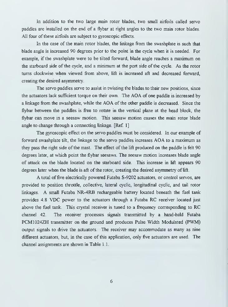
A total of five electrically powered Futaba S-9202 actuators, or control servos, are
provided to position throttle, collective, lateral cyclic, longitudinal cyclic, and tail rotor
linkages. A small Futaba NR-4RB rechargeable battery located beneath the fuel tank
provides 4.8 VDC power to the actuators through a Futaba RC receiver located just
above the fuel tank. This crystal receiver is tuned to a frequency corresponding to RC
channel 42. The receiver processes signals transmitted by a hand-held Futaba
PCM1024ZH transmitter on the ground and produces Pulse Width Modulated (PWM)
output signals to drive the actuators. The receiver may accommodate as many as nine
different actuators, but, in the case of this application, only five actuators are used. The
channel assignments are shown in Table 1.1.

Receiver Channel Output
1 Lateral Cyclic
2 Longitudinal Cyclic
3 Throttle
4 Tail Rotor
5 Rate Gyro Sensitivity Switching
6 Collective Pitch
7 (Spare)
8 (Spare)
9 Channel 9 Switch
Table 1.1. Helicopter PWM Receiver Output Channels
These actuator or servo channels are not to be confused with the radio frequency
channel assignments used on different RC vehicles. Fifty frequencies, from Channel 1 1 to
60 (72.010 to 72.990 MHz) are employed by RC enthusiasts to prevent cross-control
interference when hobbyists fly in close proximity to one another. The FROG uses
channel 26, while the helicopter came from the factory with a receiver and transmitter set
to channel 42. As we will see in a later chapter, this difference must be accounted for in
the ground control station.
In the case of the throttle, collective, lateral cyclic, and longitudinal cyclic, the
receiver output is routed directly to the actuators as shown in Figure 1.4, commanding the
actuator to rotate to a desired position.
For the tail rotor, however, the output voltage is routed to a Futaba G501
piezoelectric rate gyro which serves as a yaw damper, which can be seen on the helicopter
as a small square box located immediately aft of the receiver. The yaw damper senses
angular turn rate about the z-axis and uses this information to stabilize the helicopter in
yaw. This feature allows the RC pilot better yaw control, as all helicopters experience
considerable cross-coupling between control inputs. For example, as collective is
increased and the main rotor produces more lift, it also produces more torque for the tail
rotor to counteract. The yaw damper senses the yaw created and sends a countering
signal to the actuator, even if no input is commanded by the RC pilot.

VAlUfWtfA
FllTABA
PCM 1024
Yaw
TAIL
Hone,
Tmvmeu~i fluTOPlUT i
-J (if installed) r
i :
ctcuc>
Icvtuc \
Figure 1 .4. Futaba Receiver and Actuator Connections
The Futaba hand-held transmitter, shown in Figure 1.5, contains two primary
levers for vehicle control. The right lever controls longitudinal and lateral cyclic. Left-
right motion of the left lever of the transmitter controls the tail rotor, while up-down
motion simultaneously controls the throttle, collective and tail rotor in a predetermined
'mixture.' This mixing feature of the transmitter increases throttle as collective is
increased while adjusting the tail rotor to roughly compensate for the change in torque
created.
Figure 1.5. Futaba PCM 1024ZH Transmitter

The Futaba transmitter also has the capability to support a trainee. In this mode,
one or more of the control channels is given over to another Futaba transmitter that has
been connected to the instructor's transmitter by a training cable. The instructor pilot can
regain control at any time.

10

H. AVIONCS SUITE DESIGN
A. RAPID PROTOTYPING SYSTEM
The RFTPS has been the subject of several previous theses and only a few aspects
of this system which influence the design of the avionics suite will be presented. The
following description is based on this earlier work where the reader may find more
complete information on the RFTPS [Ref. 7,8]. Additionally, modifications to the RFTPS
required to support helicopter operations will be discussed.
1. Overview of RFTPS
The RFTPS architecture includes both the airborne sensors, required power supply
components and telemetry links, as well as a ground station. The ground station processes
sensor data and generates commands to control the vehicle.
The avionics system on board the vehicle includes a Watson Inertial Measurement
Unit (IMU), a Global Positioning System (GPS) receiver and air data sensors, such as an
altimeter or airspeed sensor. The IMU and GPS produce data through serial interfaces
that are connected to FreeWave™ wireless modems that transmit data to the ground
station. Details of these components are reviewed in Sections C, D, and E below. The air
data sensors in the FROG are connected to the IMU, and their signals are multiplexed into
the digital data stream sent to the ground station.
The RFTPS ground station contains three major components; see Figure 2.1.
First, a small "luggable" PC serves as the host for a Texas Instruments Digital Signal
Processor (DSP) which is the primary processor for executing code controlling the
vehicle. Additionally, the PC supports four hardware boards that handle input/output
(I/O) functions to support the DSP, including two serial communications modules, one
digital-to-analog module, and one Pulse Width Modulation module. [Ref. 7] The two
serial boards receive downlink data from the IMU and GPS through the pair of FreeWave
wireless modems. The Pulse Width Modulation module (IP_68332) is connected to a
Futaba receiver and allows PWM signals being transmitted to the vehicle to be captured.
The fourth hardware board is the IP_DAC module, which allows digital signals produced
by the DSP to be converted to analog voltages to drive a Futaba transmitter set in the
trainee mode.
11

The four I/O boards in the host PC are connected by ribbon cable to a
communications unit, the second major component of the RFTPS ground station. The
communications unit houses the two FreeWave wireless modems, the Differential Global
Positioning System receiver, and a Futaba PWM receiver. Additionally, this
communications unit provides a housing for these components and allows for connections
to power supplies, antennas, and the modified Futaba transmitter. This Futaba transmitter,
when placed in "trainee mode" and connected to another transmitter in the "instructor
mode" as discussed in Chapter I, is capable of communicating control signals to the
actuators on the vehicle for flight control.
UAV
Actuators IMUAir Data
SensorsDGPS
PWMCMD's
Base
Telemetry
Link 1
Telemetry
Link 2
Host PC Workstation
Figure 2. 1 . RFTPS Hardware Architecture From Ref [8]
The third major component in the ground station is the User Interface and Data
Collection Workstation. [Ref. 8] The workstation is a Sun workstation running the
Xmath / SystemBuild graphical programming software. This software allows the user to
develop control algorithms in a high-level block diagram environment and then generate
real-time code for execution on the real time processor residing on the luggable PC.
Additionally, the software supports a graphical user interface allowing the user to see
displays of parameters of interest (navigation, PWM control signals, etc.). Input
12

commands, such as altitude or heading changes, can also be entered by the user through
the graphical user interface, depending on software design. The workstation is connected
to the PC via an Ethernet TCP/IP protocol connection.
2. Ground Station Hardware Modifications
Due to the open architecture employed in the design of the RFTPS, very few
hardware modifications were required on the ground station. Since each RC vehicle,
whether it be an airplane or a helicopter, comes from the factory with a preset RF
operating channel, much as an automobile comes with a set of keys, the ground station
Futaba transmitter and receiver must be capable of operating on the RF frequency channel
of the helicopter. To allow interoperability between the FROG (channel 26) and the
helicopter (channel 42), a multi-channel synthesized receiver manufactured by Futaba
was installed in place of the crystal controlled, fixed channel receiver already in use for
the reception ofPWM signals in the ground station. Figure 2.2 depicts the new receiver.
Behind the small plastic window in the lower left portion of the receiver are two small
dials for setting the appropriate RF channel. Power to the receiver is supplied from a
power supply within the ground station, and no external battery is required.
Figure 2.2. Futaba Multi-Channel Receiver
No further hardware modifications to the Futaba transmitter were necessary. The
DB9 connector placed in the left side of the unit to allow it to be connected to the ground
station visually identifies this previously modified transmitter. The transmitter has both
13

an airplane and a helicopter mode pre-programmed into internal software. It is necessary
only to place the transmitter in this mode through the appropriate menus and to ensure
that all necessary parameters are set identically to that in the UAV pilot's master
controller when they operate in the instructor-trainee mode. The modified transmitter has
no internal RF transmitter, as it has been removed for safety purposes, and can only be
operated in the trainee mode with another Futaba transmitter.
A typical RC airplane flies with four actuators: elevator, aileron, rudder, and
throttle. A typical RC helicopter flies with five actuators: longitudinal cyclic
(corresponds to elevator), lateral cyclic (aileron), tail rotor (rudder), throttle, and
collective. Fortunately, when in the helicopter mode, the throttle and collective are
married together, as discussed in Chapter I, such that only four inputs must be made to
the modified controller from software via the DP_DAC module.
B. HELICOPTER AVIONIC SYSTEM DEFINITION
To ensure maximum compatibility with the RFTPS ground station, the helicopter
avionic system was assembled to make use of the same sensors as used on the FROG, in
so far as possible. Although the Xmath / Realsim system is capable of supporting a wide
variety of sensors, different software drivers must be written to support different sensors.
For example, a software driver has previously been written to convert serial data received
from the Inertial Measurement Unit at the serial board and process it for use by the
system. This software expects the data arriving on this link to be in binary format with
specific variables listed in a predetermined order. The software then parses this data and
assigns each portion to a different variable, such as bank angle, acceleration in the x-axis
and so forth. If a different sensor is used, new software must be written to account for the
different information format. Since any modifications to this software would then make
the system incompatible with the FROG, it was decided to use identical sensors,
wherever possible. These sensors provide all the information necessary to control the
helicopter, with the exception of an accurate low altitude data source. A later chapter
details the development of a short-range, highly accurate altitude sensor to meet this
requirement. The following sections discuss each of the other avionic components and
their respective operational capabilities, power requirements, interface parameters and
limitations.
14

C. INERTIAL MEASUREMENT UNIT
The EMU employed on the FROG, and included in the present design, is the IMU-
C604 produced by Watson Industries, Inc. The unit pictured in Figure 2.3 weighs only 2
pounds and measures 5.78" x 3.24" x 4.68" [Ref. 9]. Included in this compact package is
a solid state gyro system and solid state vibrating element angular rate sensor, as well as
two vertical reference pendulums, a triaxial fluxgate magnetometer and accelerometers.
A microprocessor collects information from these sensors and is capable of producing
output signals for bank angle, elevation angle, and magnetic heading, as well as
accelerations (x,y,z axes), and tri-axial angular rates. Additionally, the unit contains a
five channel integral analog-to-digital converter to allow the user to input analog data that
can be output along with the other measured variables.
Figure 2.3. Watson IMU-C604
Interface with the EVIU is accomplished through a 9-pin male DB-9 connector on
the forward side of the unit. This is not, however, a standard serial connection as might
be found on a PC. Table 2.1 details the pin-out for the Watson EVIU, as well as the
standard arrangement for a PC. In the Watson application, 28 VDC power to operate the
unit is provided to the EVIU through pin-2, while serial output is provided at pin-9. These
details must be accommodated when developing onboard wiring for the EVIU.
15

Pin RS232 Watson IMU-C604
1 Carrier Detect Power/Signal Ground
2 Transmit Data +28 VDC Power
3 Receive Data User A/D channel #1
4 DTR User A/D channel #2
5 Ground Receive
6 Data Set Ready User A/D channel #3
7 Not Used User A/D channel #4
8 Clear to Send User A/D channel #5
' Not Used Transmit (User receives
on this line
Table 2. 1 . RS-232 and IMU Pin Assignments
For bench testing, or to set the various output modes of the IMU, the unit can be
connected to a personal computer. Since the pin-outs of the IMU and computer differ, a
direct connection is not possible with a standard cable. A special wiring harness must be
developed to make the proper connections. The nine pins of the EMU can be connected to
a terminal strip, allowing 28 VDC power, user analog inputs for A/D conversion, and
serial communication to the PC to be connected appropriately. Most any terminal
communications program such as ProComm®, HyperTerminal® (in Windows 95), or
Crosstalk® can be employed to receive the serial output at 9600 baud (8-N-l). The IMU
Owner's Manual details how to select output formats by typing various symbols and
following prompts [Ref. 9]. The IMU can output data in ASCII decimal, hexadecimal, or
binary. If the binary mode is selected, the data will be unrecognizable, because the
terminal software interprets each byte as ASCII, and therefore prints various characters to
the screen. In addition to selecting the transmission format, the user can select which
variables are included in the output.
The choice of an output format is important because this choice effects the data
rate of the IMU. The output data transfer rate is 9600 bits per second. Internal sampling
of the analog sensor outputs occurs at 71.11 Hz. If an output format is selected which
exceeds 135 bits per sample, including start bits, stop bit, and carriage returns, there will
be insufficient bandwidth available to transfer the information. (135 * 71.11 = 9600). In
these situations, the microprocessor in the IMU selects every other internal sample for
16

transmission, or perhaps every third, fourth or fifth sample to reduce the bandwidth
required. The user can expect the IMU to provide output information at an integer
division of 71.11 Hz. For example, if ASCII format with 12 variables were selected for
output, the information would appear on a PC terminal communications program screen
as follows:
I +000.0 -01.3 304.0 -0.02 +0.00 -0.99 +00.0 +00.0 +00.0 +094 +119 +382
Notice in this case there are 71 characters in each data line plus a carriage return.
The first character is a status character followed by the 12 selected data elements. Each
ASCII character is transmitted by an 8 bit byte. However, when using the RS-232
asynchronous data communications protocol, these bits would be transmitted as part of a
frame. In this case, a single leading 'start' bit is appended before the data, and a single
'stop' bit is appended to the end. (No parity bit is sent by the IMU in this application.)
Therefore, each ASCII character requires 10 bits to be transmitted. Thus, each sample
(line of data) requires the transmission of approximately 720 bits. The IMU must select
only each sixth sample for transmission, reducing the sample rate to about 11.85 Hz.
(71.1 1 ^ 6 = 1 1.85). At this sample rate, the bandwidth required is (720 * 1 1.85 = 8532 <
9600 baud).
If, however, the binary mode is selected, each data element is a 14 bit, two's
complement format number. The first seven bits are placed in an RS-232 asynchronous
data frame (right justified), and the remaining seven bits are placed, right justified in the
next data frame. Thus, 20 bits, when start and stop bits are included, are required to
transmit each data element. Upon receipt, the user must strip off the left-most bit in each
data byte before combining them to create the 14 bit data word.
As an example, the first data element in the example data line above is bank
angle, measured ±180.0 degrees. This requires seven ASCII characters (including the
following space) which requires 8 * 7 = 56 bits to be transmitted in the ASCII mode. In
binary mode, only 20 bits need be transmitted. This analysis demonstrates that the ASCII
format, while convenient to the human observer, does not provide as efficient a
transmission format.
An important consideration when determining how to mount the IMU on the
helicopter is the orientation of the axes of the IMU. The EVIU must be installed with the
mounting base down, and the DB9 connector facing forward to align the IMU coordinate
17

system with the conventional aircraft coordinate system. Additionally, to ensure that the
internal magnetometers are not influenced by disturbances, care should be given to using
non-magnetic mounting materials and electrical connections.
As Table 2.1 describes, 28 VDC power should be provided across pins 1 and 2.
However, the unit is equipped with an internal regulator allowing operation from as low
as 24 VDC and as high as 32 VDC. Current demand is listed as about 350 mA, however,
we found current draw to be nominally 250 mA at 24 volts.
The four 16-bit analog-to-digital converters in the EMU sample at 50 Hz, and
therefore, following Nyquist, have a bandwidth of 0-25 Hz. They accept voltage inputs
from -10 to +10 VDC. In shop testing, a DC bias of about -0.08 Volts existed in the A/D
converter output. Watson reports that a single-pole anti-aliasing filter set at around 25 Hz
is incorporated into the internal design of the A/D converter.
Accelerations can be integrated to obtain velocity, and again integrated to obtain
displacement. However, this technique suffers from drift created by acceleration
measurement error. To investigate this effect, the IMU was subjected to various
accelerations and the data recorded. Specifically, the IMU was lifted from a resting
position, moved through a series of random, somewhat cyclic motions, and then returned
to its original position. This data was then introduced into MATLAB and processed
through the SIMULINK diagram shown in Figure 2.4.
Model used to Integrate IMU accelerations to get
velocity and distance.
.9954
Constant
[t M2(:,6)]
Sum1/s
Int
G_2_fps
FromWorkspace
fr[l/s|—»|dist|Int1 Output
—J velocity|
To Workspacel
Figure 2.4. SIMULINK Model Used to Twice Integrate EVIU Accelerations
The z-axis input accelerations, in g's, were corrected for the effects of gravity and
installation bias by adding 0.9954, and then multiplied by 32.2 to obtain the proper units.
The results are displayed in Figure 2.5. Notice that after only nine seconds, the error in
1!

position is nearly 3 feet. Clearly, the quality of data produced by the IMU is such that it
will be necessary to complementary filter the IMU output with an altitude source to
control this drift.
0.5
IMU-604 Responsei > i > i i i
-
-0.5
-1
S.,^ velocity
l
accel.
-1.5 I
|
-2
)
distance \-2.5 -
I"
'! j
i"'"
-i ... ,\^. _
-3C
i i i I i i
> 1 J! 3 4 5 6 7 8 £i
Time (sec)
Figure 2.5. IMU-C604 Drift
D. DIFFERENTIAL GLOBAL POSITIONING SYSTEM RECEIVER
The Global Positioning System receiver incorporated in this avionics system is
the Basic Oncore GPS Receiver manufactured by Motorola. The system provides data at
one second intervals through an RS-232 interface. The GPS system consists of the
receiver, an active antenna, and a power/data cable. These components are very compact
and lightweight, with the receiver weighing only 3.8 ounces and measuring 4" x 3" x 1".
The active antenna module is a cylindrical component 4 inches in diameter by 0.89 inches
and weighs 4.8 ounces. These components are shown in Figure 2.6. [Ref. 12]
The serial output of the device provides latitude, longitude, height, velocity,
heading, time, and satellite tracking status through a 10 pin connector that provides the
19

receiver with power as well as permitting RS-232 serial output. This output was intended
by the manufacturer to be connected to a PC running controller software, but in this
application the serial data has been used to support the software written to control the
FROG. The system requires 12 VDC power and consumes about 1.8 watts.
IBM PC OR COMPATIBLE
PC CONTROLLER(NOT SUPPLIED)
=a enr-^™ «-,
PCCONTROLLERSOFTWARE
ONCORERECEIVER
Figure 2.6. Motorola Oncore GPS Receiver From [Ref 12]
E. TELEMETRY
The RFTPS uses FreeWave™ Wireless Data Transceivers to transmit data from the
IMU and the GPS to the serial modules in the ground station. Both units operate at 9600
bps, and during flight, only the GPS requires two-way communication. The FreeWaves
may be used in any situation were a standard 9-pin null modem is used, such as
communication between two computers. The units are lightweight and easy to operate.
Table 2.2 provides information pertinent to the present application.
An important feature associated with the FreeWave system is its Gaussian
frequency shift keying (GFSK) modulation type. GFSK is a modified form of frequency
shift keying (FSK) for transmitting binary data. With FSK, a pair of transmission
frequencies are used, with one frequency representing a binary "1" and the other
representing a binary "0." The transmitter keys the appropriate frequencies in turn to
20

represent a string of bits. Immediately adjacent to this pair of frequencies in the
electromagnetic spectrum lie other possible pairs of frequencies.
Range 20 miles line-of-sight
Data Rate 1200 bps- 115.2 Kbps
Operating Frequency 902-928 MHz
Modulation Type GFSK, spread spectrum, frequency
hopping
Power 12VDC, 120 mADimensions 1.6inHx3.9inWx7.4inL
Weight 0.75 pounds
Antenna Attached 3. 5in whip or detached
Table 2.2. FreeWave Technical Specifications After [Ref. 10]
With Gaussian FSK, a Gaussian-shaped bandpass filter is placed around the pair
of interest to prevent interference from the adjacent pair of frequencies. Figure 2.7
depicts frequency shift keying.
Modulation Signal
FSK Carrier Signal
AmAFSK Spectrum
BW = 2B + (f2-fl)
Figure 2.7. FSK Frequency Pair
21

Fifteen user-selectable hop patterns cause the transmitter to hop in a
pseudorandom pattern from one pair of frequencies to another, thereby spreading the
spectrum used. Frequencies of operation run from 902-928 MHz. FreeWaves are "slow
hoppers," meaning they transmit several bits before hopping on to another pair.
Frequency hopping is one of several spread spectrum communications variants, allowing
the simultaneous use of several transmitters in the same frequency band. Internal error
detection and correction features with FreeWave prevent scrambled data in the
statistically unlikely event that two separate FreeWave transmitters hop on to the same
frequency pair together. When operating two FreeWaves pairs simultaneously, it is
important to set each to a different user-selectable hop pattern to minimize interference.
Most importantly, Spread Spectrum techniques meet the Federal Communications
Commission (FCC) requirements for unlicensed operation. Spread spectrum technology,
and GFSK modulation in particular, are in use in cellular telephones for this very reason.
[Ref. 11]
Each FreeWave transceiver, see Figure 2.8 has a serial number, or "Unit Address"
and must be programmed to operate with another serialized transceiver. This permits
multiple FreeWaves to be used simultaneously. This is useful in this application, since
two links are required.
Figure 2.8. FreeWave Wireless Modem
22

III. SONAR ALTIMETER DESIGN AND CONSTRUCTION
A. REQUIREMENTS
An aircraft traveling at 5,000 feet is adequately served with a barometric
altimeter. Aircraft routinely operate with 1000 feet of altitude separation between
aircraft. This translates to a static pressure differential of about 0.5 psi per thousand feet
in the neighborhood of 5000 feet. Measurement errors are easily tolerated. However, in
the region very close to the ground, altitude must be known much more precisely and a
barometric sensor typically does not have sufficient accuracy. For example, the
barometric altimeter on a Navy P-3C Orion aircraft can differ from field elevation by as
much as 60 feet and still be considered safe-for-flight. In pilot-controlled applications,
visual reference to the ground is used to judge altitude during the last few feet before
landing. The helicopter for this project will almost always operate well below 60 feet,
normally between the surface and 15 feet. A barometric sensor with sufficient sensitivity
to measure fractions of feet would suffer from the changing pressure levels created by the
beating rotors. These factors make a barometric altimeter such as that used in FROG
unusable for automatic control in the helicopter. The following general requirements
were developed for any altitude sensor to be used on board the helicopter:
• Usable range from the surface to 30 feet above ground level (AGL).
• Lightweight, preferably less than one pound.
• Operate on low voltage 0-24 volts DC.
• Low power, preferably in the tenths of amperes.
• Accurate within 2 inches when within a foot of the ground to allow for
computer controlled landings, and accurate within 4 inches at higher altitudes.
• Sensor output must be analog DC voltage in the range of ±10 volts to be
compatible with the internal analog-to-digital converter in the IMU. In other
words, there must be a known relationship between signal output voltage and
vehicle altitude.
• Capable of operating in the helicopter flight environment.
23

B. POLAROID 6500 SERIES RANGING MODULE
After reviewing possible alternatives, the Polaroid 6500 Series Ranging Module
was selected to serve as the core of an ultrasonic ranging system. The Ranging Module
drives an ultrasonic transducer, which serves as both a loudspeaker and a microphone for
a very high frequency sound signal. A short emission of sound consisting of 16 pulses is
transmitted which reflects off the ground and is reflected back to the transducer. By
recording the time of travel of the sound pulse and knowing the speed of sound in air, the
intervening distance can be determined. The ranging module is very light, weighing only
a few ounces, and operates on 6V DC power, drawing only 0.1 amperes. Although
limited to only about 35 feet maximum range, it can measure distances down to six
inches (lower if external blanking is employed), with an accuracy of ±1% of the reading
over the entire range.
The transducer has a very narrow beamwidth, limiting the range of bank angles at
which the transducer can receive a return signal from the ground. However, the helicopter
is envisioned to operate primarily in a hover with minimal roll inputs. Turns will be
accomplished by turning the helicopter around the main rotor using tail rotor control. In
view of the anticipated operation of the helicopter, this limitation was not seen to be a
serious problem.
The 6500 Series Ranging Module is not a ready-for-use component. As shown in
Figure 3.1, the Ranging Module is a printed circuit board with attached components
measuring less than 2 inches on a side driving a small transducer an inch and one-half in
diameter. There is no power source, on/off switch, trigger mechanism, or output signal
processing. The user must use the Ranging Module as the core in a larger system tailored
to the user's intended application. A system for repeatedly triggering the Ranging
Module and processing the output must be developed.
Figure 3.1. Polaroid 6500 Series Ranging Module and Transducer
24

Interface to the Ranging Module is through a Burndy 9-pin connector and ribbon
cable provided by Polaroid. Only seven of the nine pins are used and their functions are
indicated in Table 3.1. [Ref. 4]
Pin Number Function
1 Ground
2 Multi-echo Blanking Reset - BLNK
3 Not Used
4 Initiation - INIT
5 Not Used
6 Internal Clock - OSC
7 Echo Return - ECHO
8 Internal Blanking Cancel - BINH
9 6 Volt DC Power Source
Table 3. I . Ranging Module Pin Interface
1. Transducer Selection
There are two transducers available for operation with the 6500 Series Ranging
Module: an environmental grade electrostatic transducer, and a 7000 Series transducer.
Both are very lightweight (the electrostatic transducer weighs only 8 grams) and are of
rugged construction. The electrostatic transducer and the 7000 Series transducer require a
300 volt maximum combined voltage be applied to the transducer during transmission,
including a 150 volt DC bias and a 150 volt AC spike when discharging..
Polaroid also manufactures the 9000 Series transducer specifically intended to
operate on the exterior of automobiles and heavy-duty trucks. However, it is not
compatible with the Ranging Module and will not tolerate the bias voltage required by
the other two transducers. Additionally, it has an asymmetrical beamform, with one of
the axes presenting less than a 5 degree half-power beamwidth. Additionally, the 9000
Series transducer operates at a lower Sound Power Level (SPL) of only 1 lOdB vs. 1 18 dB
for the electrostatic transducer. [Ref. 4]
The electrostatic transducer provides greater than a 10 degree half-power
beamwidth and a circular, rather than asymmetrical beamform. Although not as ruggedly
25

designed as the 9000 Series, the technical specifications for the environmental transducer
show it is suitable for the expected conditions. Therefore, the electrostatic transducer
shown connected to the Ranging Module in Figure 3.1 was selected.
2. Ranging Module Theory of Operation
The 6500 Series Ranging Module can be operated in two different modes: a
single-echo mode and a multiple-echo mode. The multiple-echo mode is of use in
robotics when more than one object is to be detected, say one at 3 feet and one at 8 feet
from the robot. The single-echo mode is more appropriate for the SONALT application,
as only one return is expected. The single-echo mode is the default mode, as will be
discussed in detail later.
6 VDC power is applied to pin 9 continuously during system operation, while a
ground connection is provided at pin 1 . Polaroid advises that the 6 VDC supply must be
capable of providing 2.5 amperes for about 1 millisecond to support the load of the
transducer during sound transmission.
A ranging cycle is initiated by applying a 6 VDC logic signal to pin 4 (INIT).
The waveform for a typical ranging cycle is depicted in Figure 3.2. The INIT logic signal
is taken high and maintained at this level awaiting an echo return, and then reset to the
low logic level at maximum range. A period of the user's choosing can then pass before
taking INIT high once again and initiating another ranging cycle. An echo returning after
INIT has gone low will not be detected; INIT must be high to enable echo reception.
As depicted in Figure 3.2, when INIT goes high, a train of 16 pulses is emitted by
the transducer, which lasts only 0.5 milliseconds. This chirp is of very high frequency
and all that is heard by the human ear is a clicking sound. This chirp is produced at a
nominal 1 1 8 dB Sound Pressure Level (SPL) measured at 1 meter, with a minimum of
1 lOdB. The 16 pulses are transmitted at 49.4 KHz, while the range of human hearing is
from 0-20kHz. To compare the SPL of the chirp with sounds in the human range of
hearing, note that a hand-held circular saw used in carpentry emits 100 dB and that each
increase of 3 dB in SPL is a doubling of sound pressure level [Ref. 5].
The train of pulses propagates away from the transducer and reflects off the target
and returns to the transducer. Polaroid chose to use 1 6 pulses to improve detection of the
return echo. If the circuitry were designed to transmit and detect a single pulse, a single
spurious noise pulse would be considered an echo, causing an inaccurate reading.
26

Alternatively, at long ranges, a single weak returning pulse might be missed. Circuitry
designed to identify an echo based on several pulses would optimize accuracy.
Upon detection, the circuitry takes the output of pin 7 (ECHO) high, and holds it
high until INIT goes low as shown in Figure 3.2. The elapsed time between IN1T going
high and ECHO going high is directly related to the range to the target and may be
computed using a simple time-distance relation based on the speed of sound (factoring in
the round-trip distance traveled by the sound). The cycle can be repeated by returning the
INIT to low and then bringing it high again to initiate the next cycle.
INIT
Pulse
Inhib
ECHO
Figure 3.2. Waveform Logic Input and Outputs
Since the transducer serves as both a loudspeaker and a microphone, the receipt of
return echoes must be inhibited during the time the 16 chirps are transmitted.
Additionally, the transducer will continue to 'ring' after the voltage is removed, much as
a bell rings after being struck. To prevent the outgoing chirps and subsequent ringing
from being detected as a return signal, the 6500 Series Module inhibits returns during the
first 2.38 milliseconds after INIT goes high. This 2.38 msec period determines the
minimum range of the system, unless it is reset to a shorter period, as we shall see later.
This minimum distance is a function of the speed of sound in air, which is determined by
the following relation:
a2 =yRT
27

Where,
a = speed of sound (ft/sec)
y = ratio of specific heats (1.4 for air)
R = individual gas constant (1716.26 ft2/s2oR for air)
T = temperature (degrees Rankine)
Using the appropriate values for air and an ambient temperature of 70 degrees
Fahrenheit, a = 1128 ft/sec. During the 2.38 millisecond internal blanking period, the
pulses travel 2.68 feet. Accounting for round trip travel we divide by two and find the
minimum range is 1.34 feet. Temperature has an effect on the accuracy of this
rangefinding system. Take for instance the effect of an increase from 70 degrees to 95
degrees Fahrenheit. The speed of sound now changes to 1154 ft/sec, an increase of about
2.5%. This increase in the speed of sound results in a slightly greater minimum range of
1.37 feet, only a small difference. But, of more interest, is the effect of this change in the
speed of sound at a greater altitude. For an altimeter calibrated at 70 degrees, the
SONALT would underestimate altitude by about 0.5 ft at 20 ft.
The user can modify the internal blanking setting of 2.38 milliseconds with an
input at pin 8 (BINH). When BINH is taken high, internal blanking is discontinued. It is
not wise to take BINH high any earlier than the departure of the 1
6
thpulse that occurs in
the first 0.5 milliseconds. However, blanking can be reduced below the default 2.38
milliseconds to provide for low altitude operations below 1.34 feet. This would be
necessary if a control algorithm were to be developed to land the helicopter .and altitude
data was required down to a very few inches.
In the multiple-echo scheme of operations, it is necessary to reset the Ranging
Module after receiving a return from an object; otherwise the ECHO signal at pin 7
would remain high for as long as INIT is held high. Reset is accomplished by taking pin
2 (BLNK) high and returning it low again. Since the return echo may have been detected
early in the 16-pulse train, it is important to hold BLNK high for at least 44 milliseconds
to let the entire train pass before returning it low.
Although the transducer creates a very highly directional beamform concentrating
the vast majority of the transmitted energy into a narrow corridor, the sound power
density of the departing signal suffers from spreading and attenuation losses.
Additionally, only a small fraction of the transmitted energy is reflected off the target to
return to the transducer, as much is reflected off in various other directions. This posed a
28

problem to the designers at Polaroid; the receiver circuitry can only be optimized to a
small dynamic range. A very strong return produced by a nearby target would saturate
the receiver and a weak signal from a distant target might be beneath threshold if a fixed
gain amplifier was used. Since returning signal strength in this application will be
directly related to distance to the target, which is also directly related to the time since
INIT went high, a variable gain with time scheme was employed. An internal clock is
provided within the Ranging Module that steps the receiver gain through 12 steps, from a
gain of 0.25 up to a gain of 10. This allows the Ranging Module to have a much greater
dynamic range and increases the maximum attainable distance. [Ref. 4]
As indicated, the Polaroid Ranging Module requires an external power supply,
drive circuitry and output signal processing to be useful as an altimeter. A conceptual
design for this circuitry was developed to meet the requirements of this application. The
electronic expertise of Mr. Jerry Lentz, staff physicist for the Aeronautical Engineering
Department was used to perform the detailed design and physical assembly of this
circuitry. This development involved building a "breadboard" version of the circuitry,
where components such as resistors, capacitors and circuit devices were temporarily
assembled and interchanged to refine the design. Once a suitable circuit was assembled,
it was permanently mounted and soldered on a circuit card for eventual installation on the
vehicle. Mr. Lentz performed this assembly and with the aid of an oscilloscope and other
tools produced circuitry based on the conceptual design. Necessarily, the hands-on
portion of this development, including the sizing of various resistors, capacitors, and the
like, was an iterative process. The fine details of the refinement of the initial design were
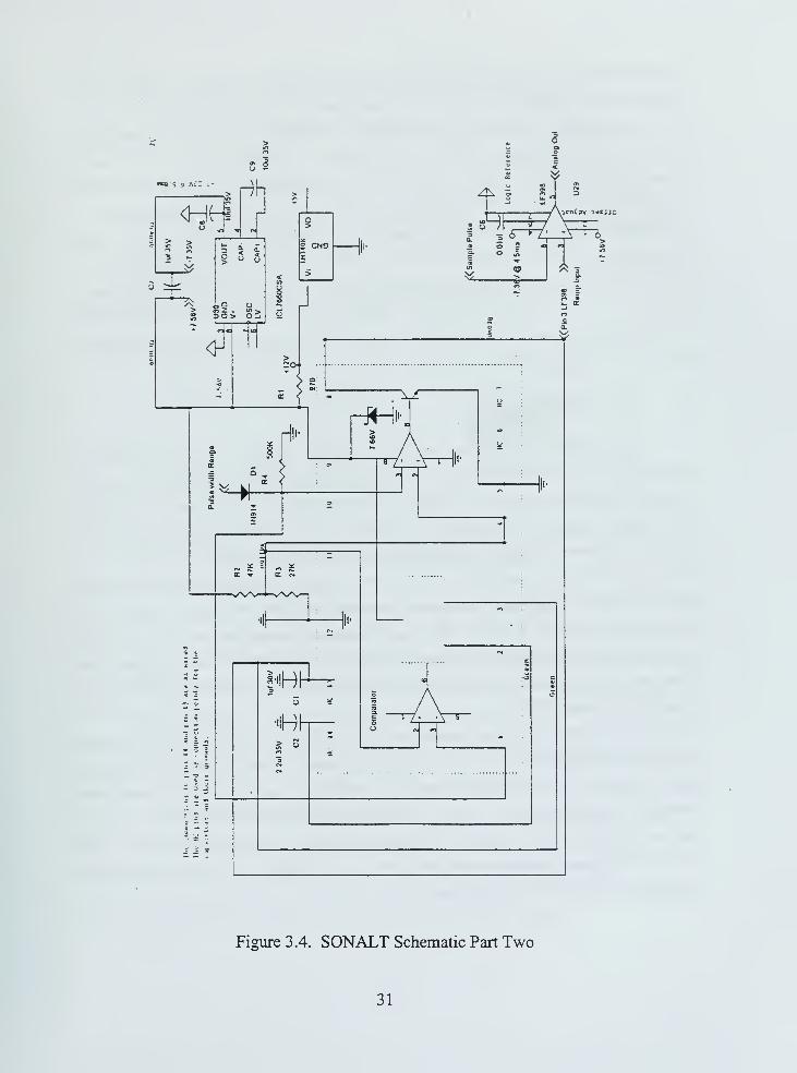
the result of Mr. Lentz's work and credit is given for his considerable efforts. Figures 3.3
and 3.4 are schematics depicting the SONALT circuitry he developed based on the initial
design. An overview of the operation of this circuitry, as developed in the initial general
design, is given in the next several sections.
C. SONALT POWER SUPPLY
The Polaroid 6500 Series Ranging Module operates on 6 VDC power. A high
capacity 12 VDC power source used to provide power to other components was available
to power the SONALT. A method for reducing the voltage without adding another large
DC converter was needed. A small LM340K linear voltage regulator was utilized on the
printed circuit card to develop approximately 5.2 VDC, which was sufficient to drive the
29

Figure 3.3. SONALT Schematic Part One
30
**8'i t ivCZ'
IcnCpv i»c;jo
Figure 3.4. SONALT Schematic Part Two
31

Polaroid Ranging Module, the oscillator and the output processing circuitry. This
component may be found on Figure 3.4 connected to the 12 VDC input supply.
As we shall see in a subsequent section, the selection of the LF398 sample-and-
hold device required both a +7V and -TV supply. A +7.56 VDC source was created by
connecting a 270 ohm resistor to the 12 VDC supply, followed by a zener diode with
voltage drop of 7.56 VDC. Thus, there was a voltage drop of 4.44 VDC across the 270
ohm resistor leaving the output of the resistor at a potential of +7.56 VDC. This voltage
was applied to an ICL7660 CMOS voltage converter to develop the -7.56 VDC required.
The ICL7660 delivers an open-circuit output equal to the negative of the input voltage to
within 0.1%. It operates by charging a capacitor (C7) connected to the input supply
voltage and also connected to the output supply, transferring the necessary charge to an
open-circuit storage capacitor (C8). [Ref. 6]
D. DRIVE OSCILLATOR
An oscillator is needed to repeatedly trigger the Ranging Module to produce an
acoustic pulse. Several different types of oscillators are available which produce specific
types of waveforms: sinusoidal, sawtooth, and triangle waves are examples. A sinusoidal
wave may be produced by a simple LC circuit. However, the Ranging Module requires
the wave to consist of only two voltage levels, and not the continuously varying voltage
of a sinusoidal wave. In addition to a DC power input, the Ranging Module requires the
INIT logic input to be taken high (about 5-6 volts) and then low (about zero volts) for
each cycle. This would be seen in the time domain as a rectangular waveform. Polaroid
recommends using a simple oscillating circuit consisting of two Schmitt triggers, which
accept standard Transistor to Transistor (TTL) logic inputs. The drive circuit developed
is depicted in Figure 3.5.
The two Schmitt triggers are depicted as triangles with small circles on the right-
hand vertex, which identify them as inverters. Inverters perform a basic logic function:
given low logic input, the inverter outputs a high logic output. Figure 3.6 shows six
inverters incorporated together into a single Dual In-line Package (DIP). A supply
voltage must be provided at pin 14 and a ground at pin 7. It is standard practice to omit
this supply voltage on diagrams such as Figure 3.5. This undepicted voltage is the source
of the output voltage for low logic input.
32

1k 1/8W1K
R1
47uf Tantalum
R5
+ C1
White
74LS14
U1B
74LS14
Figure 3.5. Rangefinder Oscillating Circuit
vccSN54/74LS14
14 13 12 10
)
^d L^>b \^3
l>p \\Pp fiPp14
GND
Figure 3.6. Motorola 74LS14 Schmitt Trigger DIP
Although an inverter is depicted by the symbology of a triangle and an appended
circle, the internal circuitry in the Schmitt trigger is made up of several components
providing the performance the manufacturer desires. Although the Schmitt trigger
internal arrangement is not this elementary, its operation may be roughly understood by
the following example. A simple inverter can be made of a NPN transistor and a resistor
as shown in Figure 3.7. A transistor operates as a switch, and is controlled by applying a
current to the base, labeled "A" in the figure. Whenever a voltage greater than an
established value is present at the base, current flow is enabled (the "switch" is on)
between the collector and the emitter (from the resistor to ground). This "pulls-down"
the voltage at A-bar to close to ground potential. Thus an inversion has been created; Ais high, and A-bar is low. When no current flow is present from base to emitter, the
"switch" is off, and there is no flow of current through the transistor from collector to
emitter. Therefore, the voltage at A-bar remains high, while A is low.
33

Figure 3.7. Simple Inverter
Referring again to Figure 3.5, we see that at start-up, the input to the left-hand
inverter (U1A) would be low, since the capacitor is not charged and no other power
source is available. This causes the inverter U1A to produce a high output. Current
flows through the variable resistor R5 and through resistor Rl to begin charging the
capacitor CI. The rate at which the capacitor charges may be controlled by setting the
values of the two resistors and the capacitor. When the capacitor charges to the point
where the voltage sensed at the input (pin 1) reaches about 0.6 V, the output is then
switched low. The charge on the capacitor is then drawn down through pin 2, bringing
the input to low logic again. This repeated switching from high to low creates an
oscillating output which may be used to drive the Ranging Module at pin 4 (INIT) after
being inverted by a second inverter (U1B). Due to the values of the resistors and
capacitor chosen, an asymmetric pulse was created at pin 2 of U1A as shown in Figure
3.8. Also shown is the signal at the output of pin 4 of U1B, which is used to drive pin 4
(INIT).
A pulse repetition frequency (PRF) of 1 Hz was chosen for the oscillator based
on several factors. First, the RFTPS control software operates at a discrete sampling rate
of 25 Hz; a PRF of greater than 25 Hz would be wasted effort. Secondly, because INIT
must be held high while the signal is propagating out and until it returns to the transducer,
a minimum value for the INIT being high is related to the maximum range desired. Since
the stated requirement was an altitude range from zero to 30 feet, the INIT must be high
for a minimum of:
(2 x 30 ft) h- (1 128 ft/sec) = 53 milliseconds.
34

An optimum solution might be to hold INIT high for 53 milliseconds and then
bring it low for 2 milliseconds before going high again. This 55-millisecond pulse
repetition interval (PRI) corresponds to about an 18 Hz PRF, close to the software
sampling rate of 25 Hz. However, Polaroid recommends INIT be held low for as long as
100 ms for proper operation. This period was considered to be excessive and
experimentation revealed that a shorter INIT low period was satisfactory. A 1 Hz PRF
made a good compromise and good results were achieved during ground testing.
UlApin2
UlBpin4
25 ms
75 ms 75 ms
Figure 3.8. Oscillator Waveforms
A combination of the two resistors and one capacitor was chosen so the oscillating
waveform created at pin 4 remained high for 75 ms and then went low for about 25 ms.
The resulting PRI was 100 ms, which corresponds to a 10 Hz PRF. A variable resistor
was employed to allow the user to fine tune the oscillator and adjust for variations caused
by temperature.
E. OUTPUT SIGNAL PROCESSING
Altitude is determined by measuring the time between INIT going high and
ECHO going high. By applying the speed of sound and accounting for round trip travel,
an accurate altitude may be computed. Since the EMU is being used to transmit the
altitude information to the ground station through an analog-to-digital input channel, the
SONALT output must be in a form compatible with that unit. The IMU analog-to-digital
converter accepts analog voltage from 10V to -10V. Analog circuitry was developed to
convert the information contained in the high/low logic waveform produced by the
Ranging Module to an analog voltage proportional to altitude.
35

A two step process was envisioned. First, using logic gates on integrated circuits,
AND the INIT signal with an inverted ECHO signal to produce a Pulse Width Modulated
(PWM) signal. The resulting PWM waveform, as shown in Figure 3.9, will have the
same PRI as the INIT signal (100 ms). The length of time the pulse is high (pulse width)
is directly related to altitude. Note in Figure 3.9 the altitude is increasing, as shown by
the pulse width of the PWM signal increasing with time.
INIT
Echo
Echo
PWM
Ramp
/I100 ms
^ w
Figure 3.9. PWM Range and Ramp Waveforms
Secondly, the PWM waveform is processed to generate a voltage. This is
accomplished by creating a ramp waveform where the voltage increases linearly with
time until the PWM pulse goes low. This ramp waveform is sampled at its peak and the
voltage measured is held until the next sample is taken during the next PRI. The details of
these two steps will be discussed in the following subsections.
1. PWM Waveform Creation
The Schmitt trigger oscillator previously discussed is located in the upper left-
hand corner of Figure 3.3. The output of pin 4 of U1B of the oscillator can be traced to
its connection with the Polaroid Ranging Module, and also be traced to pin 1 of U2A,
which is an AND gate on a 7408 TTL integrated circuit. The ECHO return from the
36

Ranging Module is inverted and then connected to pin 2 of U2A. The output at pin 3 is a
PWM waveform. However, during the assembly of this circuit, it was noted that the 16
pulses of the echo appeared at the beginning of this PWM waveform. Additionally, there
was a period of "dead-time" in the echo pulse due to the latency of the Ranging Module
circuitry to produce and detect a pulse. In other words, even at zero range, the ECHO
return from the Ranging Module does not appear for a short period. In order to trim the
16 pulse artifact and dead-time period from the beginning of this PWM waveform, the
waveform is again AND'ed at U2D with a delayed version of the INIT signal. This
delayed INIT signal is produced by a diode Dl, the capacitor C2, and the two inverters,
U1F and U1E. Capacitor C2 is charged by the leakage current coming out the input of
the Schmitt trigger. Since the INIT signal was delayed by about 0.75 milliseconds, it
may be used to reset internal blanking by inputting this signal to pin 8 (BINH) of the
Polaroid Ranging Module allowing altitudes as small as 5 inches to be measured. Recall
that all 16 pulses are transmitted in the first 0.5 milliseconds.
2. PWM Waveform to Voltage Conversion
The design developed determines a voltage corresponding to altitude for each
pulse of the altimeter, and continues to produce this voltage until another return is
received. When plotted against time, the desired output voltage would appear as a
stairstep pattern, with each step lasting 100 milliseconds. The first step in creating this
stairstep involves creating a ramp waveform such as depicted in Figure 3.9. The ramp
waveform is the sampled at its peak, and that output held until the next sample is taken.
See Figure 3.10.
The LM2917 Frequency to Voltage Converter is a fourteen-pin device intended
for use in tachometer circuitry. In this application, however, individual components
inside the device are used to create the ramp waveform. The components of the LM2917
are shown within the dotted lines in Figure 3.4. Incidentally, note that the zener diode
used for +7.56 VDC voltage regulation is a component on this device. Most useful for
creating a ramp waveform are the charge pumps. The Pulse Width Range is brought in to
the LM2917 at pins 10 and 1 through diode Dl. In tracing the connection through pin 1
of LM2917, we see the PWM Range signal is an input to a comparator, which drives two
charge pumps.
37

Ramp
Sample
and hold
/I
_|1
Figure 3.10 Sample and Hold
These charge pumps can be viewed as ideal current sources. They produce
current at a constant rate regardless of voltage and thus can be used to charge a capacitor
linearly with time, rather than exponentially. The comparator senses a constant reference
voltage through pin 1 1 . When the PWM range signal applied to pin 1 is high, the charge
pumps provide a positive current to charge capacitors C2 and CI, which have been
mounted on pins 14 and 13 of the LM2917 for convenience. Capacitor CI has been sized
so that at approximately 55 milliseconds (approx. 30-foot range) the capacitor is charged
to five volts and because a charge pump drives it, the charge increases linearly with time.
This produces the required ramp. Note the connection in Figure 3.4 between capacitor
CI and the sample-and-hold device, LF398.
The LF398 sample-and-hold circuit has been depicted in both Figures 3.3 and 4.4
for clarity. The device is supplied with ±7 VDC supply voltage at pins 1 and 4, while the
ramp input waveform is connected at pin 3. When a sample pulse is applied at pin 8, the
device samples the ramp waveform voltage and outputs this voltage steadily until the next
sample pulse, even if the input ramp waveform subsequently is reset. In this case, the
sample pulse must be applied at the very peak of the ramp, just prior to the ramp being
reset for the next cycle. A complication in this design is that the instant the sample pulse
is needed is dependent on the altitude, which is precisely the unknown quantity to be
measured.
38

Returning now to the PWM range output of pin 1 1 of U2D on Figure 3.3, we can
follow the creation of this sample pulse. U1D produces an inverted form of the PWMwaveform while diode D2, capacitor C5, and U3C produce a 20 (isec delayed version of
the PWM waveform. This delay is produced in a manner similar to the process used to
create a delayed version of the oscillator by U1F and U1E. The AND gate U2C
combines these two waveforms as shown in Figure 3.11 to create a 20 (isec sample pulse
which begins just after the PWM waveform falls. This sample pulse is input to the
sample-and-hold device, LF398, at pin 8.
The sampling occurs just before the ramp input is pulled low by a NPN transistor
at pin 8 of the LM2917 device. The base of this transistor is connected to a comparator,
which compares the PWM waveform to a reference voltage. When the PWM waveform
at pin 1 goes low, the comparator applies a voltage to the base of the transistor pulling
pin 8, and the ramp input down in preparation for the next cycle.
Delayed
PWM
PWM
Sample
Pulse
20
1
-n 5
<-
Figure 3.11. Sample Pulse Waveforms
Expansion capability was provided in that a spare AND gate and three inverters
are still available to allow an additional Ranging Module to be added.
39

F. TRANSDUCER MOUNTING
Several factors influenced the design of the mounting for the transducer. The
transducer is essentially a thin piece of foil stretched across a grooved backplate to form
the moving element that creates sound from an input voltage, and then converts returning
sound into electrical energy [Ref. 4]. This foil has been reported to be very sensitive to
vibrations. Additionally, as noted earlier, a very high voltage is placed across the
transducer during each transmission, which would likely induce noise into other electrical
components and wiring on the vehicle. Furthermore, the transducer must be mounted
with a clear path to the ground.
A lightweight aluminum frame was developed, across which a sheet of rubber
could be stretched, and pressure plates attached to hold the rubber sheet securely to the
frame, as shown in Figure 3.12. The transducer is fitted in an undersized hole cut in this
rubber sheet, allowing the transducer to be firmly attached. This aluminum frame, or
mount, is attached below the aluminum deckplate on the underside of the helicopter to
prevent electrical noise from penetrating up to avionics installed on the deckplate.
P&' -
:
*, W5 i
ii
V 1
!
1
1 B • mm-
1 j
Figure 3.12. Transducer Mount
G. SONALT TESTING
Testing involved mounting the transducer on the side of a box to allow sound
signals to be emitted horizontally towards a flat wall. The SONALT circuitry was driven
by the same 12 VDC converter used on the vehicle to ensure conditions close to those in
flight could be duplicated. The analog output voltage from the SONALT circuitry was
connected to the "IMU Word 4" input channel to the IMU. The serial output was then
connected to a laptop computer to record and display the voltages measured by the A/D
converter. This equipment was placed on a cart and rolled from a position very close to
the wall out to maximum range, stopping at intervals to record data. The minimum range
40

proved to be about 5 inches where voltage reached a minimum. Further decrease of range
resulted in the same voltage value. Data was recorded at 1-inch intervals for the first
foot, and then measurements were made at one-foot intervals to 25 feet. Additional
measurements were made at 30 feet and greater. The maximum range was measured at
about 32 feet, beyond which a constant voltage was produced.
Detailed data are provided in Appendix A. The results appear to be quite linear,
however a linear fit through the data produces an error of nearly four inches at ranges less
than a foot. A fifth order curve-fit produced very small coefficients for all but the linear
terms, but was able to reduce error to less than an inch. The following relationship was
developed:
alt = -0.0026*5 + 0.0475*
4 - 0.3 15x3 + 0.9524*
2 + 5.0434x + 0.6764
Where x is the input voltage and altitude is measured in feet. This equation can
be implemented easily in the RFTPS software to obtain altitude in feet. Figure 3.13 plots
the data recorded with a polynomial curve fit.
SONALT Cal Fifth Order
35
y = -0.0026xs + 0.0475X
4- 0.31 5x
3 + 0.9524x2 + 5.0434X + 0.6764
R2 =1 y>30
25
?ncoucn»Q 1*
10
*
Voltage
Figure 3.13. SONALT Calibration
41

Additionally, the SONALT's tolerance to angle-of-bank deviations was tested by
positioning the transducer 10 feet from a wall and progressively tilting the transducer
until the return was no longer detected. At this close range, the maximum deviation was
measured as 16 degrees. This wall was very smooth and hard and tended to reflect all
signals such that the angle of incidence equaled the angle of reflection. An uneven
ground surface might improve this limitation, although soft ground might not reflect
energy as well as the hard wall.
The results provided in Figure 3.14 were recorded during a test run where the cart
was moved across the floor towards the wall while continuously recording data. The run
began at nearly 30 feet from the wall and continued for approximately 23 seconds.
During this time period the data appeared smooth and was uninterrupted by any bad data
points or outliers. When inspected in a short time scale, the jagged appearance of the data
can be seen to be stairsteps of about 100 milliseconds, just as expected.
SONALT GROUND TEST
0.99 1.97 2.96 3.94 4.93 5.91 6.9 7 88 8.87 9.85 10.8 11.8 12.8 13.8 14.8 15.8 16.7 17.7 18.7 19.7 20.7 21.7 22.7
Time (sec)
Figure 3.14. SONALT Ground Test
42

IV. AVIONICS RACK AND POWER SUPPLY DESIGN
A. REQUIREMENTS
The basic helicopter, while possessing a lift capability in excess of 20 pounds (as
discussed in Chapter I), does not provide for any cargo area or suitable enclosure to house
the avionics suite. A platform of sufficient size to carry the necessary components with a
large margin for future growth was needed. A test flight with 1 5 pounds of steel plate
attached to the landing skid was performed to confirm the advertised lifting capacity.
Test flight results revealed that the 15 pound payload required a very small increase in
collective at trim and the UAV pilot felt confident that 20 pounds could easily be lifted.
Several factors influenced the ultimate design of the avionics platform:
•The physical volume needed to mount the equipment.
•The presence of the pull-starter on the underside of the helicopter.
•The need to place the DVIU on centerline as near to the CG as possible.
•Weight and structural strength.
•Ease of construction and availability of materials.
A method of mounting the components and sensors on the helicopter and
providing power was developed. The location of each component was determined and its
effect on the vehicle center of gravity was assessed. Additionally, to ensure adequate
protection from vibration, methods for isolating sensitive equipment were examined.
B. SKID DESIGN
Two options to mount components were available. First, a framework or platform
could extend laterally from the helicopter. With a support structure loaded with
equipment covering the flanks of the helicopter, access to the pull-starter would be
severely restricted, since only 4 inches clearance would be available to reach under the
laterally mounted rack and grasp the pull-starter handle. Additionally, the EVIU would be
mounted off-center, although the effects of this displacement could be accommodated
with a software transformation. With components loaded outboard, the carburetors on the
starboard side would be obscured, and heat shielding would be necessary on the port side
adjacent to the exhaust. The existing plastic landing skid could be retained.
43

The second option, and the option selected, was to build a framework below the
helicopter to serve as both an avionics rack and landing skid. The IMU could be mounted
on centerline, and a large flat surface would be available to mount electronic components.
Ample room would be available under the nose of the helicopter for the future installation
of a camera. The pull-starter could easily be reached, and access for an electrically
powered starter shaft could be provided through the bottom of the rack to replace the
hand starter.
Available materials were inventoried and a large stock of Vi inch aluminum
channel was located. Engineering drawings were produced and the landing skid shown in
Figure 4.1 was constructed with 308 square inches of surface area. All joints were
welded except where the skid rails attach to the legs below the avionics platform, which
were attached with screws for easy removal. Connection between the helicopter frame
and the avionics rack was accomplished through the use of attachment plates on the upper
rack cross-members. These mounting plates formed a sandwich which mated with the
composite chassis at the same holes provided for the original plastic landing gear. 0.050"
aluminum sheeting was used for the platform deck and was attached to the aluminum
frame with screws. The total weight of the rack and skid assembly was 5.65 pounds,
including an access tube provided for the starter. This left a useful payload of more than
fourteen pounds available for avionics equipment.
Figure 4. 1 . Aluminum Avionics Rack and Landing Skid
C. COMPONENT PLACEMENT
Placement of components on the avionics rack was primarily influenced by
weight and balance considerations. An overhead view of the placement of components
44
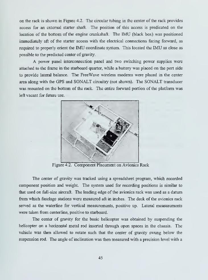
on the rack is shown in Figure 4.2. The circular tubing in the center of the rack provides
access for an external starter shaft. The position of this access is predicated on the
location of the bottom of the engine crankshaft. The IMU (black box) was positioned
immediately aft of the starter access with the electrical connections facing forward, as
required to properly orient the 1MU coordinate system. This located the EVIU as close as
possible to the predicted center of gravity.
A power panel interconnection panel and two switching power supplies were
attached to the frame in the starboard quarter, while a battery was placed on the port side
to provide lateral balance. The FreeWave wireless modems were placed in the center
area along with the GPS and SONALT circuitry (not shown). The SONALT transducer
was mounted on the bottom of the rack. The entire forward portion of the platform was
left vacant for future use.
\
®^ / -41
.
\/
Mm Ik
v-y -.„
IrA
Figure 4.2. Component Placement on Avionics Rack
The center of gravity was tracked using a spreadsheet program, which recorded
component position and weight. The system used for recording positions is similar to
that used on full-size aircraft. The leading edge of the avionics rack was used as a datum
from which fuselage stations were measured aft in inches. The deck of the avionics rack
served as the waterline for vertical measurements, positive up. Lateral measurements
were taken from centerline, positive to starboard.
The center of gravity for the basic helicopter was obtained by suspending the
helicopter on a horizontal metal rod inserted through open spaces in the chassis. The
vehicle was then allowed to rotate such that the center of gravity swung below the
suspension rod. The angle of inclination was then measured with a precision level with a
45

built-in protractor. Several different suspension points were used, and the intersection of
the lines-of-position was plotted to determine the center of gravity. As shown in
Appendix B, the center of gravity was located directly below the rotor mast, as expected,
at a point located 14.25 inches aft of the leading edge and 12.4 inches above the avionics
deck. A similar procedure was followed to obtain the center of gravity for the avionics
skid alone. This information, along with component weights and positions was recorded
in the spreadsheet and the final position of the center of gravity determined.
The spreadsheet program allowed several different component arrangements to be
considered and the effect on the movement of the center of gravity quickly determined.
The top of the horizontal stabilizer on the tail of the helicopter was chosen as the
location for the GPS antenna for two reasons. The device weighs only 4.8 ounces, but a
position this far aft is helpful in maintaining the center of gravity near the rotor mast.
Additionally, this location provides a more unobstructed horizon for the antenna and is
somewhat removed from the electrical noise generated by other avionics and the spark
plugs of the engine.
D. POWER SUPPLY SYSTEM
The components incorporated into the design of the avionics suite must be
steadily supplied with a power. Pertinent data is listed in Table 4. 1
.
Component VDC Amperage (mA) Watts
IMU 24 250 6.00
FreeWaves (2) 12 240 2.88
GPS 12 150 1.80
SONALT 12 150 1.80
Total 12.48
Table 4. 1 . Avionics Power Budget
A MILSPEC battery (BA-5590/U NSN 6135-01-036-3495) of the same type used
in the FROG was selected due to its ability to produce 24 VDC power, as well as its
availability. The battery consists of two 12 volt cells enclosed in a single casing.
Linking these two cells in series can create a 24 volt source. Batteries are typically rated
in milliamp-hours (mAh). This battery is rated 14,400 mAh when wired in series [Ref.
46

15]. The 12.48 watt load described above requires 520 milliamps at 24 volts. Even when
accounting for the converter efficiency (probably around 80 %), the battery is clearly
capable of supporting the intended application. Two batteries of this type are used by the
Marine Corps in its AN/PSC-3 man-pack mobile satellite communications package,
which is capable of transmitting 35 watts ofpower [Ref. 13].
Battery voltage decreases over time as components continue to draw power.
Additionally, the voltage in a system is drawn down temporarily when one component
draws peak power. Household plumbing systems are a useful analogy. Water pressure is
everywhere influenced by the demands of one faucet or shower. Two voltage converters
were selected, identical to those used on FROG: one producing a constant output of 24
VDC with an input voltage anywhere within the range of 18-36 VDC to support the IMU.
A second converter creating 12 VDC with input voltage 18-36 VDC supports the
remaining avionics. The converters are rated at 2 amps and 2.5 amps respectively, fully
adequate for the demand. These converters aren't simple transformers. A transformer
uses a ratio of windings around a magnetic core to step voltage up or down by the ratio of
the windings. These converters are switching regulators capable of maintaining a
constant output voltage throughout a range of input voltages.
A power supply panel was assembled upon which the converters, associated
switches, test points, and connectors were mounted. The supply panel is shown in Figure
4.3.
Figure 4.3. Power Supply Panel
A single-pull, double-throw switch allows selection of either an external 24 VDCpower source for ground testing and maintenance, or the internal 24 volt battery. 24
47

VDC and 12 VDC switches control the output of the two converters, and an extra switch
for future use was provided. 24 VDC external power may be attached through a
MILSPEC three pin female connector. Additionally, a female DB9 connector was
provided on the panel face to allow access to the IMU to adjust the unit's parameters
stored in EEPROM (Electrically Erasable Programmable Read Only Memory). The
panel mounted serial connector can also be used to sample data directly from the EMU to
a laptop computer as described in Chapter II, without unplugging the connector from the
IMU. On the interior side of the power panel, a terminal strip was provided for easy
connection to the IMU's A/D converters. Wiring diagrams for the power supply system
and for signal connections are contained in Appendix C.
E. VIBRATION ISOLATION
Although vibration caused by the main and tail rotors, as well as vibration
produced by the engine and reduction gearing was anticipated, it proved to be a much
greater problem than anticipated. Sensitive electronics, such as the IMU, and later, a
camera, need to be protected from the harsh vibrations produced by the helicopter. The
reduction gearing between the engine and the main rotor provides a ratio of 90:14, while
the tail rotor turns at roughly 4.5 times faster than the main rotor. Since the helicopter
has a two-blade main rotor, it was expected that there be a predominant vibration
frequency at the main rotor RPM, called "IP" for "once per" revolution of the main rotor,
and also a strong artifact at double that frequency, called "2P." The vibration frequency
spectrum was determined with three different test procedures.
First, a small, hand-held RPM reader produced for the RC enthusiast was used to
measure the RPM of the main rotor blade while in flight. The device has a small
window, similar to the viewfinder on a camera, through which the operator is able to
view the blades of the helicopter in flight. The device operates much like the timing
strobe on an automobile used by mechanics. The operator of the RPM reader adjusts the
frequency of the strobe to make the main rotor appear to stop when viewed through the
rangefinder. When this condition is reached, the rotor RPM can be read off an LCD
display. This measurement produced a reading of 1570 RPM (26.2 Hz). A single blade
passes a fixed point with a frequency of 26.2 Hz, however, with two blades on the main
rotor, spectral components will also be seen at 52.4 Hz.
48

A second test was conducted using a three-axis accelerometer mounted on the
helicopter and connected via an umbilical to a spectrum analyzer. The spectrum analyzer
revealed high energy around 28 Hz and 56 Hz. 28 Hz equates to a main rotor RPM of
1680 RPM. A later test revealed a main rotor frequency of about 27 Hz. Note that the
RPM will vary with the lift and collective required to hover, which in turn vary with air
density and current weight of the helicopter. Therefore, the variation in readings can be
traced to variations in weather conditions, fuel weight, avionics weight, collective/throttle
settings, and engine performance. The vibration spectrum for the later test is plotted in
Figure 4.4.
1000
900
800
I I
700
600
500
400
300
200
100 II : n
1 ! 1 Jc
ilWWk*um) 10 20 30 40 50 60
Frequency (Hz)
70 80 90 1()0
Figure 4.4. Vibration Spectrum
The 27 Hz main rotor frequency was selected as a design point for the purposes of
vibration isolation. The power transmitted at this frequency and at the higher 2P
frequency of 54 Hz is far greater than the other vibration frequencies measured. Rubber
mounts are available to isolate equipment from vibrations. To achieve proper isolation,
however, the proper mount must be selected for the application. In addition to providing
49

protection from the periodic vibrations caused by the main rotor blades, these mounts
provide protection against damage to equipment caused by shock, such as a hard landing.
Initially, consideration was given to isolating the entire platform, such that all
components mounted on the platform would be protected. This approach is complicated
by the need to evenly distribute weight across the several mounting points to achieve
proper vibration isolation. If components are not flown on a particular flight, for example,
the loading would become uneven, and the expected isolation would not be achieved.
Therefore, since not all components require shock mounting, it was decided that only the
most sensitive equipment would be shock/vibration mounted.
To determine the proper mount for a particular application, it is useful to consider
the avionics component and the associated mounts as a simple spring-mass-dashpot
system as shown in Figure 4.5.
k
Mass = m
^1-
1 *
b
-1 x,
Figure 4.5. Simple Spring-Mass-Dashpot System
In this system, the vibrating structure causes a deflection across the spring that
transmits a force to the supported mass. The nature of the motion produced is a function
of the mass of the component, the spring constant (k) of the mount, and the damping (b)
afforded by the mounting material. The platform vibration is considered an input to this
system, and is represented as x;. The response of the component is represented by x<>. The
transfer function from input to output is:
ff(5) =bs + kXo(s) _
Xi{s) ms 2+bs + k
50

Where s = jco, where co is the periodic frequency of the vibration in question in
radians per second. Notice that for a very small excitation frequency, H(s) is very nearly
one. This means the mass would follow the motion of the base. If however, the input
vibration frequency were to be very high, H(s) would be very small, indicating that the
motion of the mass would be very small.
In this case, a mount with a certain k and b must be selected such that IP and 2P
frequencies are greatly attenuated. Lord Mechanical Products produces a series of
lightweight mounts such as shown in Figure 4.6. A mounting arrangement of four
1 00PDL-A mounts was selected, with one mount at each corner of the IMU. Each mount
is rated at 0.5 pounds capacity with a spring constant k = 8 pounds per inch = 96 pounds
per foot. No value for the damping constant (b) is published. Lord Mechanical Products
advises that these mounts are manufactured from an elastomeric material, which differs
from the common steel spring in that its stiffness changes with the rate of deflection, not
simply with distance. This gives the elastomeric mount the properties of a spring and also
a damper. Damping is thought to be rather light, and is assumed to be about £, = 0.1,
lacking more detailed specifications.
Figure 4.6. Elastomeric Platform Mount for IMU
Inserting the values for the variables and dividing the numerator and denominator
of the transfer function above by the value of the mass, we find the characteristic equation
in the denominator. The IMU weighs just 2 pounds (0.0622 slugs) and the spring constant
51

constant k must represent all four mounts and is expressed in pounds per foot, (k = 8 * 12
* 4 = 384 pounds/ft) The resulting characteristic equation is:
b 384s + s + =
.0622 .0622
Therefore, the natural frequency, co n is:
384 _7Q<-7(°" ~
V "0622~
(Radians/sec)
Assuming damping % = 0.1, the second term of the characteristic equation must
become:
2£a>n s = 2(.l)(78.57)s = 15.7b
The transfer function then becomes:
»w- 5+6ms2+15.71s + 6173
A bode diagram for this transfer function is given in Figure 4.7. Notice that at
lower frequencies the gain from input to output is slightly greater than one, or dB. The
gain increases, reaching a peak at about 78 rad/s, the natural frequency of the system.
The computed natural frequency of the mounts was confirmed by testing. The height of
this peak is a function of the amount of damping in the system — the more damping, the
lower the peak. From the peak, the gain decreases, crossing the dB point at a value of
1.414 times the natural frequency. The region from DC to the axis crossing point is
known as the region of amplification. As frequency continues to increase, the gain
steadily decreases. This region is known as the region of isolation. The computed
natural frequency was confirmed through laboratory testing. The elastomeric mounts
were placed on the IMU and the EVRJ was displaced from its neutral resting position and
then released. The response was measured. A spectral analysis of the accelerations
revealed a peak around 13 Hz (81 rad/s).
The 100PDL-A mount was chosen because IP and 2P, at 27 Hz (170 rad/s) and 56
Hz (339 rad/s) respectively fall in the region of isolation. This was the lowest cutoff
52

frequency available using off-the-shelf mounts. The gain at IP and 2P can be computed
by substituting jco for each frequency into the transfer function. IP (27 Hz) has a gain of
about -1 1.34 dB and 2P (54 Hz) has a gain of -24.91 dB.
Figure 4.7. Bode Diagram of Elastomeric Mounts on EMU
The region of amplification makes the choice of mount in an avionics application a
compromise. If the disturbing frequencies are known, then a lightly damped system with
the natural frequency located well below the disturbing frequencies would be a best
choice. In this application, however, there will be a time as the rotor RPM is increased for
takeoff, that the predominant vibration frequencies passes through the natural frequency of
this lightly damped system. During this period prior to takeoff, EMU data may be
unusable for flight control.
53

54

V. INITIAL FLIGHT TESTING AND SYSTEM MODIFICATION
A. INITIAL FLIGHT TESTING
Due to delays in fabrication of the aluminum avionics frame, the development of
the SONALT and assembly of the power panel were completed in parallel with the
construction of the frame. The avionics rack was first flown without any components
attached. See Figure 5.1. Recall that earlier lift-capacity testing involved strapping thick
metal plating to the stock plastic landing skids without noticeable vibration or adverse
effect on handling qualities. However, upon lift-off with the avionics rack installed, a
severe vibration developed in the newly created helo-avionics rack system. The
attachment plates at the top of the avionics rack were connected to the bottom of the
composite material used in the chassis of the basic helicopter. In this area, the composite
material proved to be quite flexible and allowed the avionics rack to vibrate laterally with
such violence the helicopter was immediately landed. As it hovered, the engine and rotor
appeared fairly steady, while the rack vibrated below.
Figure 5.1. Helicopter with Vacant Avionics Rack
The new overall vehicle structure created by the addition of the avionics rack
contained vibration modes that were excited by the main rotor frequency and/or
associated harmonics. The flexibility of the chassis composite material allowed motion
and no practical method was available at this late stage to "soften" the structure, to isolate
the rack from rotor and engine vibration. It was thought that by stiffening the structure
with supports, the natural frequency of the structure could be increased to a frequency
well above the main rotor frequency. Therefore, four lateral supports made of thin
55

aluminum tubing were attached, two to a side, to stiffen the structure as shown in Figure
5.2.
Figure 5.2. Avionics Rack Lateral Supports
The helicopter was then flown to assess the effect of the structural changes.
Instead of reducing the vibrations, the lateral supports served only to change the nature of
the vibration, and caused much of the vibration energy to propagate out the tail boom. A
videotape of the flight revealed extensive shaking of the entire frame and twisting of the
tailboom and reduction gearing. Again the helicopter was quickly returned to the deck.
It became evident the solution to the vibration problem would not be an easy one.
Blade tracking and blade balance were checked and were found within limits. A
subsequent flight of the helicopter in its original configuration showed no excessive
vibrations. Awaiting an acceptable solution to the problem of how to mount the avionics
components, a modification of the avionics system was conceived.
B. SYSTEM MODIFICATION
To prove the operation of the SONALT inflight, and collect limited acceleration
data, a small avionics package was developed consisting of the SONALT circuitry and
transducer, a three-axis accelerometer, and associated power supply. The analog outputs
of these sensors would be transmitted to the deck via an umbilical or tether, and there
connected to the avionics rack. The rack would be located in the vicinity of the hovering
56

helicopter. Figure 5.3 shows the arrangement with the modified avionics package
mounted just below the fuel tank on the nose of the helicopter.
4 -
SOMaaias
life-
5.3. Helicopter with Modified Avionics '.
The three-axis accelerometer used was built by Crossbow Industries and has a
bandwidth of 100 Hz for accelerations from -4 to +4 g's. It requires 5 VDC power and
produces a DC signal output from to 5 VDC. A 2.5 VDC output represents zero g's,
with roughly a 0.5 VDC per g calibration. For example, a 3 VDC output voltage would
represent roughly 1 g.
An aluminum box was constructed to contain the SONALT and the
accelerometer, along with the required 12 VDC power source for the SONALT. Since 5
VDC power is needed for the accelerometer, a simple linear regulator was used to convert
the necessary 5 VDC power. The SONALT circuit board was placed inside the box along
with a power supply box and a terminal strip, as shown in Figure 5.4. Eight AA-cell
batteries were used to supply 12 VDC power. Each cell is rated at 2800 mAh, providing
ample power and lifetime.
Batteries produce the 12 VDC required for flight operations, however, a three
position switch was provided to allow the selection of external power for ground
operations and testing, as well as battery power. The center switch position removes
power from both sensors. 12 VDC external power is provided through a 5mm audio style
jack. The terminal strip was installed to allow easy disassembly of the unit, when
necessary. Analog output voltages are routed out of the box through a multipin connector
to a five conductor, shielded cable used as an umbilical. A wiring diagram of this
avionics package is included in Appendix D. Table 5.1 gives color coding for the
umbilical wiring.
57

Vs.
!/
Figure 5.4. Internal View of Modified Avionics Package
Color Signal IMU Channel
Red X acceleration Channel 1
Black Y acceleration Channel 2
White Z acceleration Channel 3
Green Altitude Channel 4
Bare wire Ground N/ATable 5.1. Umbilical Wire Connections
The transducer mounting originally designed to be attached to the bottom of the
avionics rack was attached to the bottom of this aluminum box, with wiring routed
through a 0.5 inch hole with protective grommet.
This, lightweight (1.86 pounds) package was then mounted below the fuel tank on
the helicopter with layers of foam rubber providing vibration insulation on the top and
rear of the aluminum box. The umbilical cable was routed alongside the starboard skid
rail and then inboard to a centerline position very nearly below the center-of-gravity. A
thirty-foot length of umbilical connected the helicopter to the remaining components on
the avionics rack on the deck as shown in Figure 5.5.
58

Figure 5.5. Avionics Rack Supporting Umbilical Flight
Under this arrangement, the components on the avionics rack performed just as
they would in flight, with the four analog voltages being fed into the EVIU through the
terminal block to the IMU's internal A/D converters. This information was then
transmitted by the FreeWave wireless modem to the ground station, where it was
recorded along with PWM signals sent to the aircraft during flight.
Due to the vibration problems encountered during early test flights with the skid,
more detailed acceleration information was desired. Data is recorded by RFTPS software
at 25 Hz, and by Nyquist, is unable to preserve information greater than 12.5 Hertz.
Although a single pole anti-aliasing filter with a 20 Hz cutoff frequency is provided in the
IMU prior to A/D converter sampling, the roll off on this filter is such that 27 Hz main
rotor vibrations are attenuated only slightly before sampling and create strong aliasing in
the resulting accelerometer data. Therefore, a method of recording digital data with a
higher sampling rate was required to accurately reconstruct the spectrum of vibration.
This information will be helpful to further investigate vehicle vibration.
A Tattletale® Data Logger was attached to the analog signal outputs available on
the avionics skid. The Data Logger was programmed to sample the four channels at 200
Hz and output data through a serial interface to a laptop computer. Single pole lowpass
filters were installed prior to sampling. The cutoff frequencies of the filters were set at 23
Hz for channels 1-3, and 160 Hz for channel 4.
59

C. PWM TO BLADE ANGLE CORRESPONDENCE
As discussed in Chapter II, the RFTPS ground station has the capability to capture
transmitted signals from the Futaba transmitter and record this information
contemporaneously with flight data received through the FreeWaves. Futaba receivers
produce PWM waveforms for use by the actuators. PWM signals may be reduced to a
numerical value by measuring the length of the pulse in microseconds. This data,
however, is useless, unless it is known what position the various flight controls on the
vehicle correspond to a given PWM value.
In conjunction with Matt McEwen, whose thesis work involved the development
of a linear model of this helicopter, relationships were developed between pulse duration
and blade position for collective, lateral cyclic, longitudinal cyclic, and tail rotor through a
series of measurements [Ref 14]. Due to a broken wire in the ground station, collective
PWM measurement was not possible. However, since the relationship between throttle
and collective due to mixing by the Futaba transmitter was known, it was possible to relate
collective blade angle with throttle PWM. It is important to note, that due to presence of
the yaw damper between the PWM receiver on the helicopter and the tail rotor actuator,
actual tail rotor blade angle may differ in flight from that called for by PWM. Moreover,
due to mixing in the transmitter, tail rotor blade angle also varies with the position of the
collective control to a small degree.
Measurement of blade angle for a given PWM signal was accomplished using a set
of levels specifically designed for the task. The helicopter was first leveled fore and aft
with a small level placed along the tail boom, and the flybar was secured in a level attitude
with the use of a brace. The main rotor blades were thereby positioned athwartships.
Recall that flybar position has an effect on blade angle, and by fixing the flybar at a level
attitude, consistent measurements can be produced. Figure 5.6 shows the leveling
process.
Next, a commercially produced level was placed on a main rotor blade as shown in
Figure 5.7. This level measures the angle of the blade chord line with respect to the earth.
It was then possible to use the Futaba transmitter to advance the rotor blade through the
range of operation one-degree at a time while recording the associated PWM with the
RFTPS ground station. Appendix E includes detailed results obtained from these
measurements.
60

Figure 5.6. Leveling in Preparation for Blade Angle Measurements
The plots ofPWM versus blade angle were linear in all cases and a simple linear
regression analysis produced the following relationships. For collective blade angle in
degrees versus throttle PWM:
AOA = -.0208 * PWM +33.31
For Longitudinal Cyclic:
AOA = .0263 * PWM -40.274
For Lateral Cyclic:
AOA = .01184*PWM-18.26
For Tail Rotor:
AOA = -0.0981 * PWM +151.324
Figure 5.7. Blade Angle Measuring Level
61

During later test flights (see Chapter VI), PWM was measured and averaged
during a stable hover. Table 5.2 contains trim values for the basic helicopter and 1.8
pounds of payload.
Control Actuator Trim PWMLongitudinal Cyclic 1594
Lateral Cyclic 1558
Tail Rotor 1491
Throttle 1504
Table 5.2. Flight Control Trim PWM Values
D. REALSIM SOFTWARE MODIFICATIONS
Thus far, activities have revolved around developing hardware for use on the
aircraft compatible with the ground station hardware and software. Next, software
modifications will be discussed. The RFTPS uses the MATRIXX Product Family of
software. The Graphical User Interface (GUI) that ties the various components of this
software product together is called RealSim. Zanino [Ref 7] and others have written
extensively about the architecture of this software.
A copy of the most current version of the software written for FROG was obtained
and stored in a separate directory on the ground station SPARC so that changes could be
made without effecting the FROG. The RealSim software provides an Interactive
Animation Editor, allowing the user to build custom pages for display on the monitor
during flight testing. These pages are constructed using a library of dials, gauges, and
digital readouts that can be attached to variables in the software. In this way, current
output parameters can be displayed to the screen and user inputs may be commanded
through the use of the mouse and keyboard.
Using the Animation Editor, a new page specifically designed to support testing of
the SONALT and accelerometer sensor package was developed and is shown in Figure
5.8. Data displayed are: altitude measured by the SONALT, PWM commanded by the
Futaba transmitter, and accelerations measured by the three-axis accelerometer. Both raw
data in volts (microseconds in the case ofPWM) and the computed values are displayed.
Raw EMU A/D converter data are assigned variable names, "wordl_imu" through
"word4_imu," corresponding to the channel assignments shown previously in Table 5.1.
62

Using the intuitive block format used to build a system in Xmath, these variables can be
tracked to theADMJ Superblock, where equation blocks convert these voltage values
to g's (for accelerometer data) and feet (for the SONALT).
Altitude8.00 Volt*
8.00 P««t
Long. Cyclic
L*t«r«l Cyclic
T*>11 Rotor
8.00 volts8.oo G's
Flight Controls
PWM Blade Angle
8.00 s.OO
8 .00 8 . 00
8.00 8.0 Approx.
8.00 8. 00
Acceleration^
Y8.00 Volts
8.00 G's
SENSOR TEST
Xi-^ltn-l™.
z8oo Volts
8.00 G's
Figure 5.8. RealSim Sensor Test Animation Page
In a similar manner, the PWM data is assigned variable names TP7 through TP15.
Table 5.3 shows the assignment of these variables. These variables may be tracked
through the block diagrams to the CommandTx Superblock, where the equations
developed above convert the PWM data into the associated blade angle. In the case of
PWM and IMU data, the newly created variables can be accessed by the Animation Editor
for display during flight test. Appendix F contains the modified Superblock diagrams
performing these conversions and creating the new variables.
Additionally, variables of interest for flight test, such as EVIU data, altitude data,
accelerations, and PWM may be selected using the Data Acquisition editor collection to
file for use in post-flight analysis. This information may be converted to an ASCII text file
from Xmath through the use of the "save" command with appropriate keywords at the
Xmath command line for use in other software packages for analysis.
63

With the modified avionics box now mounted on the helicopter and the data
retrieval equipment ready to record data via the tether, the helicopter was flown and the
quality of data was assessed.
Variable Name Actuator
TP7 Longitudinal Cyclic
TP8 Lateral Cyclic
TP9 Not Used
TP10 Trainer Light
TP11 Tail Rotor
TP12 Not Used
TP13 Throttle
TP14 Collective (Not functional)
TP15 Not Used
Table 5.3. PWM Variable Assignments
64

VI. AVIONIC SYSTEM TESTING
A. FLIGHT TESTING
Flight testing was conducted for two purposes. First, data was collected to assess
the performance of the SONALT and three-axis accelerometer. Additionally, flight test
data was used to validate a linear model of the helicopter produced by Matt McEwen
[Ref. 14]. The modified avionics package was mounted below the helicopter fuel tank and
tethered to the avionics rack on deck. Data was fed to the ground station by a FreeWave
modem where it was captured by the RealSim Data Acquisition Editor. The ground
station was capable of capturing the three-axis accelerometer signal voltages, and the
SONALT signal voltages through the IMU A/D converter, along with the PWM signals
being sent to the helicopter by the pilot. These data are recorded at 25 Hz. Additionally,
the Tattletale data logger was connected to the terminal strip on the avionics rack to
collect data, which was subsequently transferred to a laptop computer via serial link. The
data was collected at 200 Hz, and was limited to 38.46 seconds due to available memory.
Once the data buffer was filled, a short period was required to transfer this information to
the laptop for hard disk storage.
Due to the data limit on the data logger and to synchronize the recordings of the
two systems, a series of separate data collection sessions was devised, each session
focusing on a specific maneuver. Both data collection systems were started together and
data recorded until the Tattletale buffer was full. During the collection session, prebriefed
maneuvers were performed by the UAV pilot as shown in Figure 6.1. Each data
collection session is reviewed in the following section.
Figure 6.1. Avionics Package Test Flight
65
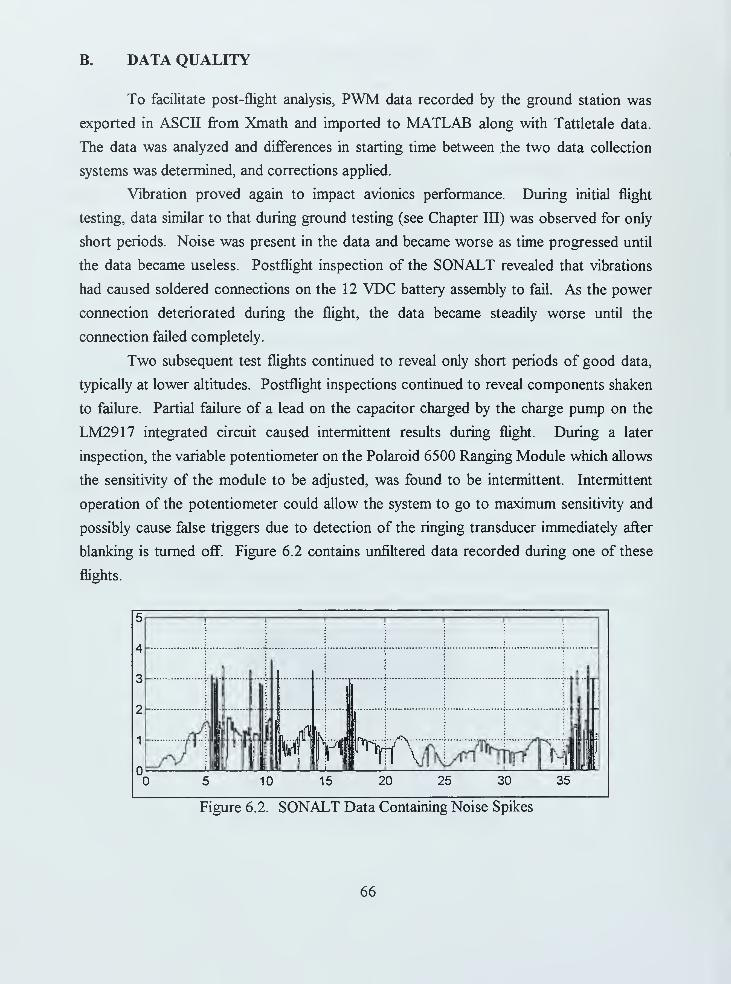
B. DATA QUALITY
To facilitate post-flight analysis, PWM data recorded by the ground station was
exported in ASCII from Xmath and imported to MATLAB along with Tattletale data.
The data was analyzed and differences in starting time between the two data collection
systems was determined, and corrections applied.
Vibration proved again to impact avionics performance. During initial flight
testing, data similar to that during ground testing (see Chapter III) was observed for only
short periods. Noise was present in the data and became worse as time progressed until
the data became useless. Postflight inspection of the SONALT revealed that vibrations
had caused soldered connections on the 12 VDC battery assembly to fail. As the power
connection deteriorated during the flight, the data became steadily worse until the
connection failed completely.
Two subsequent test flights continued to reveal only short periods of good data,
typically at lower altitudes. Postflight inspections continued to reveal components shaken
to failure. Partial failure of a lead on the capacitor charged by the charge pump on the
LM2917 integrated circuit caused intermittent results during flight. During a later
inspection, the variable potentiometer on the Polaroid 6500 Ranging Module which allows
the sensitivity of the module to be adjusted, was found to be intermittent. Intermittent
operation of the potentiometer could allow the system to go to maximum sensitivity and
possibly cause false triggers due to detection of the ringing transducer immediately after
blanking is turned off. Figure 6.2 contains unfiltered data recorded during one of these
flights.
Figure 6.2. SONALT Data Containing Noise Spikes
66

The general path of flight can be discerned by "eyeball integration" of the data, but
large transients are present when the altitude is greater than one foot. The altitude drops
to zero on this graph during these transients. The graph is produced from Tattletale data
which does not record negative voltage values, but the ground station does. Where the
Tattletale shows zero, the ground station showed negative voltage.
Faulty components were replaced and the remaining components were checked
and where possible reinforced with silicone sealant to prevent vibration failure. Data
quality improved significantly and an analysis of the results is provided below. Detailed
data is provided in Appendix G.
1. Vertical Doublets
Figure 6.3 contains test data taken with the UAV pilot commanding collective
control doublets after a period of generally level flight. The data appears much improved
with fewer noise spikes. Occasional drops in data last for 100 ms each, indicating that the
drops are the result of a single PRI. Examination of the slope of the doublets reveals a
high rate of climb and subsequent descent, through which the altimeter tracks well. Most
of the data drops occur in the vicinity ofthese maneuvers, however.
Figure 6.3. Unfiltered Altitude During Vertical Doublet Maneuvers
An analysis of this data reveals that most of the sharp transients are drops in
altitude from an altitude of several feet down to an altitude below one foot. Furthermore,
these drops very frequently last for one altimeter cycle, or 100 ms, before returning back
to near the previous altitude. Analog techniques such as low-pass filtering can also help
smooth high frequency transients, but the cutoff frequency required to adequately suppress
these transients begins to effect the good data as well. The graph in Figure 6.4 contains a
67

spectral analysis of the altitude data from an early flight where electrical component
failures created many transients. A large spike can be seen in the area of 5 Hz. This is
because the data often dropped to zero for 100 ms, jumped to a high value for 100 ms and
so forth. This created oscillations with a period of 200 ms (5 Hz). A filter with a cutoff
frequency of only 2 or 3 Hz would be necessary to smooth the data. This filtering would
cause the peaks on the doublets in Figure 6.3 to be reduced in height and delayed in time.
700Altitude Spectrum f3_523
600-
500
400-
300
200
100
JSh i ,Jhl*Lk!kkmk*Jlht.L -JK,
10 20 30 40 50 60 70 80 90 100Frequency (Hz)
Figure 6.4. Altitude Data Spectral Analysis
An advantage to digital signal processing is that non-frequency based filter
techniques can be employed easily. For example, computer code was written to analyze
each data element and compare it with the previous data point. If the data drops from an
altitude greater than one foot to an altitude below one foot, that point, along with all
points during the next 100 ms cycle can be ignored, using the previous value instead.
Additionally, each data point can be averaged with the previous seven points (previous
.035 seconds) to smooth transients. Figure 6.5. presents the results of such a filter.
68

Figure 6.5. Filtered Altitude During Vertical Doublet Maneuvers
Acceleration and PWM actuator control signals were also analyzed. Figure 6.6
depicts z-axis (vertical) accelerometer data.
0.5 h
"5-0.5
to -1
-1.5
-2
-2.510 15 20 25
f529-1 Vertical Doublets
30 35
15 20Time (sec)
Figure 6.6. Z-Axis Accelerometer Data During Vertical Doublet Maneuvers
Top: raw data, Bottom: filtered data
Note that the z-axis is defined as positive down. The raw data in the top graph
contains high frequency noise generated by the helicopter engine and rotor system and the
overall acceleration of the vehicle is not apparent. A fourth order Butterworth low-pass
69

filter was employed with a cutoff frequency of 40 radians/sec (6.4 Hz) to remove the 27
Hz (IP) and 54 Hz (2P) spectral components. The accelerations corresponding to each of
the three doublet maneuvers can be clearly seen. The results are provided in the bottom
graph in Figure 6.6.
As described in Chapter V, the PWM varies inversely with collective blade angle
on this helicopter. An increase in PWM causes a decreased blade angle. Figure 6.7
depicts altitude and PWM information for the vertical doublet maneuvers. This
information can be used to develop or validate a mathematical model of the helicopter.
15 20 25
f529-1 Vertical Doublets
35
1700
1650
140010 15 20 25
Time (sec)
30 35
Figure 6.7. PWM Measurements During Vertical Doublet Maneuvers
2. Lateral and Longitudinal Doublets
Lateral and Longitudinal Doublets were performed to gather accelerometer
information to support Major McEwen's model identification work, but the altitude data
collected is also useful in assessing SONALT performance. Filtered and unfiltered data for
the lateral doublet maneuver is provided below in Figure 6.8.
70

f529-2 Lateral Doublets
15 20Time (sec)
Figure 6.8. Unfiltered Altitude During Lateral Doublet Maneuvers
As the UAV pilot performed these maneuvers, the altitude information was
recorded. While performing these maneuvers, the pilot's primary attention was placed on
creating the lateral and longitudinal inputs required, and naturally, altitude varied through
these maneuvers. This data reveals a potential cause of bad data points. Although not
evident from the altitude data in the vicinity of 12 seconds in Figure 6.8, the helicopter
was completing a lateral motion to the left and had rolled to the right when the drop in
data occurred. Longitudinal data (see Appendix F) also revealed dropped data during
maneuvers, probably associated with vehicle pitch. Recall that the SONALT transducer
produces sound energy in a narrow beam of only 10 degrees, as discussed in Chapter III.
Due to the narrow beamwidth, as the vehicle pitches or rolls, the gain of the transducer
and the amount of energy reflected to the vehicle from the ground is decreased, reducing
71
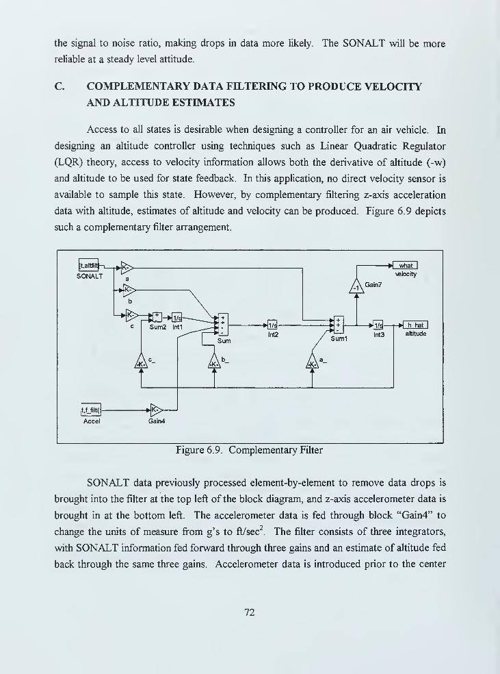
the signal to noise ratio, making drops in data more likely. The SONALT will be more
reliable at a steady level attitude.
C. COMPLEMENTARY DATA FILTERING TO PRODUCE VELOCITY
AND ALTITUDE ESTIMATES
Access to all states is desirable when designing a controller for an air vehicle. In
designing an altitude controller using techniques such as Linear Quadratic Regulator
(LQR) theory, access to velocity information allows both the derivative of altitude (-w)
and altitude to be used for state feedback. In this application, no direct velocity sensor is
available to sample this state. However, by complementary filtering z-axis acceleration
data with altitude, estimates of altitude and velocity can be produced. Figure 6.9 depicts
such a complementary filter arrangement.
;t,altfi
SONALT3^1*^
-£>
L,^ffl-^Sum2 Int1 -HS-
M what I
velocity
Gain7
t,f_filt(
Accel
•£>-J
Int2
+&Sum1
Int3
»j h hat I
altitude
Gain4
Figure 6.9. Complementary Filter
SONALT data previously processed element-by-element to remove data drops is
brought into the filter at the top left of the block diagram, and z-axis accelerometer data is
brought in at the bottom left. The accelerometer data is fed through block "Gain4" to
change the units of measure from g's to ft/sec2
. The filter consists of three integrators,
with SONALT information fed forward through three gains and an estimate of altitude fed
back through the same three gains. Accelerometer data is introduced prior to the center
72

integrator. An estimate for altitude is produced at the output of the third integrator, and
an estimate for velocity can be produced from the input to the third integrator.
Installation bias is accounted for in this filtering scheme. In other words, if the
three-axis accelerometer is not perfectly aligned to the aircraft body axis, an error in z-axis
acceleration would be present. Instead of reading a value of -1.0 g (gravity only,
measured with respect to the downward-pointing z axis) with the helicopter at rest on a
level surface, for example, the reading might be -0.99 g. If a simple integration of
acceleration were conducted to obtain a velocity estimate, this difference would
compound over time causing a large velocity error. With the use of three integrators in
this filter, the left-most integrator "learns" this bias error and outputs a value to
compensate for it.
Consider the steady-state condition where the vehicle is at constant altitude and
zero vertical velocity (w = 0). An examination of Figure 6.9 reveals that feedback values
would equal feed-forward values at each of the summers. Due to the opposite signs
provided on the summers for these inputs, their effects neutralize one another. Also at
steady-state, the left-most integrator produces a value of equal magnitude to the
acceleration being input. Therefore the input to the right-most integrator would be zero
and the altitude estimate unchanged.
The values for each of the feed-forward and feedback gains is related to the
bandwidth of the SONALT and three-axis accelerometer. The values for a, b, and c are
computed through the following relation, where x is the bandwidth of the SONALT.
(s3 + as
2 +bs + c)=\ s + -V T
J
Since the SONALT operates at a PRF of 10 Hz, it may have a bandwidth no
greater than 5 Hz by application of the Nyquist theorem. Several values for x were
evaluated and x = 2 Hz produced acceptable results. By inserting a value of x in the
equation above and expanding the right-hand side, the gains may be computed by term-by-
term comparison. Gains computed were a = 37.7, b = 473.8, and c = 1985.
Flight data from the longitudinal doublet maneuvers was filtered and the results are
provided in Figure 6.10. Note that the velocity, w, is positive when the vehicle is
descending, which is proper in the aircraft coordinate system used. The velocity
information produced tracks well with altitude and is usable for controlling the helicopter
with a LQR controller.
73

Figure 6. 10. Altitude and Velocity Estimates Produced by Complementary Filter
74

VH. CONCLUSIONS AND RECOMMENDATIONS
A. OVERVIEW
This thesis has touched on broad areas fundamental to avionics development:
avionics sensor selection, power requirements, mounting and vibration protection,
telemetry and communications, digital and analog interfaces, data acquisition, and circuit
design and testing. Much remains to be accomplished beyond the initial steps taken.
B. SPECD7IC COMMENTS
1. Sonic Altimeter
The precision altitude measuring system designed for compatibility with the
RFTPS was proven to be a successful approach for this application. Much more testing
remains to be accomplished, however. The doublets performed during flight testing
provided data for modeling, but were not the sort of maneuvers that would typically be
performed under computer control. Hovering operations without abrupt maneuvers
should be performed to obtain a better measure of SONALT performance. Once telemetry
is installed and altitude is no longer restricted, maximum range should be determined. The
effects on performance of different surfaces (ground, pavement, etc.) should be
investigated. The narrow beamwidth of the altimeter limits vehicle pitch and roll, yet these
limits have not been precisely determined. Future flight test could determine these limits
and perhaps test different approaches, such as the use of multiple transducers set at
different angles to accommodate pitch or roll. Polaroid provided a variable potentiometer
on the 6500 Series Module to allow the user to adjust the sensitivity of the transducer.
Test flights should determine what sensitivity setting is appropriate for optimum
performance. In summary, the sonic altimeter is usable as a precision data source for
control of the vehicle in a hover at low altitude. With the use of the three-axis
accelerometer and complementary filtering, vertical velocity can be estimated.
2. Avionics Mounting and Vibration Control
The most challenging aspect of this project was not an avionics issue, per se, but
rather the task of mounting the components on the helicopter and providing the
75

appropriate protection from vibration. The avionics rack developed compounds the
vibration problem and provides no cushion on landing. A more sophisticated approach
should be investigated, perhaps involving disassembly of the current helicopter and
replacing the composite chassis with a new structure capable of supporting avionics. The
use of a shaker table and advanced finite element computer modeling might aid the
development of a more suitable mounting scheme. Alternatively, following the lead of
some commercial vendors, a mounting system which connects to the bottom of the plastic
landing skid might permit the vibrations to be dampened by the plastic skid. This work
might involve more detailed flight testing and analysis of the vibrations present and
subsequent design by a student with aircraft structure and vibration experience.
3. Avionics Package Weight Reduction
Mr. Kelly Johnson, the lead aircraft designer at Lockheed Skunk Works and
developer of the F-104, U-2, and SR-71 aircraft was fanatical about reducing aircraft
weight. He concerned himself with design changes resulting in only a few pounds on an
aircraft of several thousand pounds gross weight. Weight also plays an important factor in
the performance of this helicopter. Although this helicopter has considerable weight
lifting capability, the reduction of weight in the avionics system will greatly aid vibration
isolation.
Several areas for weight reduction are available. The DC switching converters,
power distribution panel and the battery weigh four pounds. The converters are
electrically oversized for the load drawn, and any further reductions in power requirements
due to the choice of different sensors could allow lighter converters to be used. The
MILSPEC lithium battery is not rechargeable. Due to the short flight endurance of the
helicopter (about 20 minutes), smaller rechargeable batteries could be incorporated in any
design.
Considerable telemetry bandwidth is currently wasted. The FreeWave wireless
modem may be set to as high as 115 KBPS; only 8.3% of capacity is being used to
support the EMU. A multiplexing scheme could be employed to take the two parallel
transmission paths of the FreeWaves, and combine them into one serial stream.
76

4. Data Quality First Priority
Quality data is essential to the proper performance of an automatic controller.
Sensors other than those used on the RFTPS should be investigated to determine if better,
more lightweight, more energy efficient sensors are available that are more suitable for the
present application. Before making any attempt to control the vehicle with software,
emphasis should be placed on developing a complete sensor system capable of providing
the data of sufficient quality. Lightweight miniature sensors and electronics such as the
Tattletale data logger should be examined for airborne use, since the low power
consumption and capability of such hardware can greatly enhance data collection.
5. Controller Design
It is recommended that further flight testing be done to provide altimeter and
vertical acceleration data to develop a model of the helicopter altitude dynamics. Once a
quality model is obtained, altitude control can be attempted using the existing modified
avionics package. Further modeling of the autopilot (not yet installed) could lead to
development of heading, speed, and position controllers.
6. RFTPS Ground Station
A separate ground station should be constructed to support the helicopter. A new
ground station designed to receive information from the sensor suite on the helicopter
could be devised, and with modification of the various drivers, still allow use of the
existing software.
C. SUMMARY
Much was learned about the performance characteristics of the helicopter and its
basic vibration and aerodynamic qualities. This information should serve as a firm
foundation for follow-on research with the helicopter. A successful SONALT has been
developed which can be used to control the helicopter.
77

78

LIST OF REFERENCES
1
.
Schluter, Dieter., Schulter 's Radio Controlled Helicopter Manual, p. 26,60. Argus
Books Limited, 1981.
2. Futaba PCM1024ZA Instruction and Operation Manual, Futaba Corporation of
America, Irvine, California, 1993.
3. Helicopter Owner 's Manual, Bergen Machine & Tool, Inc., Wisconsin, March 15,
1997.
4. Biber, C, The Polaroid Ultrasonic Ranging System: Operations Manual, p. 5.
Polaroid Corporation, Ultrasonic Components Group, Cambridge MA.
5. Sound. The World Book Encyclopedia, 1985; 18:490.
6. Principles and Applications ofthe ICL7600 CMOS Voltage Converter, p. 11-11,
Harris Semiconductor Corporation, April 1994.
7. Zanino, James A., Uniform Systemfor the RapidPrototyping and Testing of
Controllersfor UnmannedAerial Vehicles Master's Thesis, Naval Postgraduate
School, Monterey, CA, 1996.
8. Hallberg, Eric N., On Integrated Plant, Control and Guidance Design Doctoral
Dissertation, Naval Postgraduate School, Monterey, CA, 1997.
9. IMU-C604 Owner 's Manual, Watson Industries, Inc., Eau Claire, Wisconsin, August
1995.
10. FreeWave User Manual, VS. 4, FreeWave Technologies, Inc., Boulder, Colorado,
1996.
1 1
.
Chayat, Naftali, Frequency Hopping Spread Spectrum PHY of the 802. 11 Wireless
LAN Standard, p. 2, Presentation to IEEE 802,
http://grouper.ieee.org/groups/802/ 1 1 /main, html . 11 March 1996.
12. Oncore GPS Receiver Quick Start Kit Manual, p. 5, Motorola, Inc., 1995.
13. Marine Corps Order 2100.3'A, Commandant ofthe Marine Corps, 26 June 1989.
14. McEwen, Matt, Dynamic System Identification andModeling ofa Rotary Wing
Unmanned Aerial Vehiclefor Stability and Control Analyssis Master's Thesis, Naval
Postgraduate School, Monterey, CA, 1998.
79

15. Military Battery Specifications, Eternacell Power Conversions Inc., May 1998http://www.eternacell.com/sDec mil. htm
80

APPENDIX A. SONALT CALIBRATION DATA
Voltaqe 1Distance (ft) Polvfit(ft) <Close-up (ft) Overall (ft) IPolvfit 4th (ft)
0.028 0.41666 0.2990026 0.4105984 0.1137464 0.395182911
0.044 0.5 0.3943747 0.4952832 0.2146872 0.480374015
0.061 0.58333333 0.4957523 0.5852608 0.3219368 0.571248968
0.078 0.666666 0.5971761 0.6752384 0.4291864 0.662489539
0.093 0.75 0.6867061 0.7546304 0.5238184 0.743295774
0.109 0.833333 0.7822443 0.8393152 0.6247592 0.829795127
0.125 0.916666 0.8778234 0.924 0.7257 0.916606567
0.136 1 0.9435578 0.9822208 0.7950968 0.976468449
0.326 2 2.0820215 1.9878528 1.9937688 2.03218479
0.508 3 3.1779593 2.9511424 3.1419704 3.078135274
0.68 4 4.2185458 3.861504 4.227084 4.093161748
0.838 5 5.1785993 4.6977664 5.2238744 5.044835081
0.992 6 6.1181867 5.5128576 6.1954296 5.987379708
1.153 7 7.1045348 6.3649984 7.2111464 6.985915779
1.296 8 7.9840813 7.1218688 8.1133048 7.882071169
1.464 9 9.0215694 8.0110592 9.1731832 8.943758462
1.625 10 10.020061 8.8632 10.1889 9.968132739
1.793 11 11.066381 9.7523904 1 1 .248778 1 1 .04226888
1.926 12 11.897917 10.4563328 12.087849 11.89523653
2.1 13 12.990059 1 1 .37728 13.18558 13.01326179
2.26 14 13.998597 12.224128 14.194988 14.04233343
2.42 15 15.011226 13.070976 15.204396 15.07147566
2.56 16 15.900633 13.811968 16.087628 15.97153585
2.73 17 16.984837 14.711744 17.160124 17.06351
2.89 18 18.009483 15.558592 18.169532 18.09011977
3.02 19 18.84502 16.246656 18.989676 18.92346727
3.19 20 19.94172 17.146432 20.062172 20.01245045
3.35 21 20.978128 17.99328 21.07158 21.03706981
3.5 22 21.953475 18.7872 22.0179 21.99804375
3.65 23 22.932418 19.58112 22.96422 22.96020728
3.82 24 24.046233 20.480896 24.036716 24.05333659
3.96 25 24.96696 21.221888 24.919948 24.95684573
4.72 30 30.019844 25.244416 29.714636 29.96881153
4.88 31 31.095371 26.091264 30.724044 31.06170925
5.02 32 32.039812 26.832256 31.607276 32.03374863
Figure A. 1 . SONALT Calibration and Curve Fit Data
81

SONALT Calibration
35
30
25
y = 6.3088X - 0629
R2 = 0.9996^^
Voltage
Figure A. 2. SONALT Linear Curve Fit
82
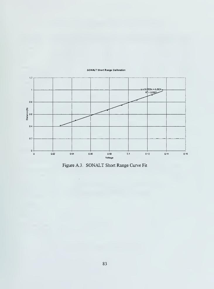
1 2
0.8
c 06
SONALT Short Range Calibration
y = «; : otry + n 9K94 .
R- = 0.9^3,'
02 004 0.06 008
Voltage
1 12 0.14 0.16
Figure A3. SONALT Short Range Curve Fit
83

SONALT Cal Polyfit Fourth Order
35
£20
y :0.0149x4 -0.1649x3 + 0.e
R2 =
"" "
624x2 + 5.2774X + 0.2469
1 uS
Voltage
Figure A.4. SONALT Fourth Order Curve Fit
84
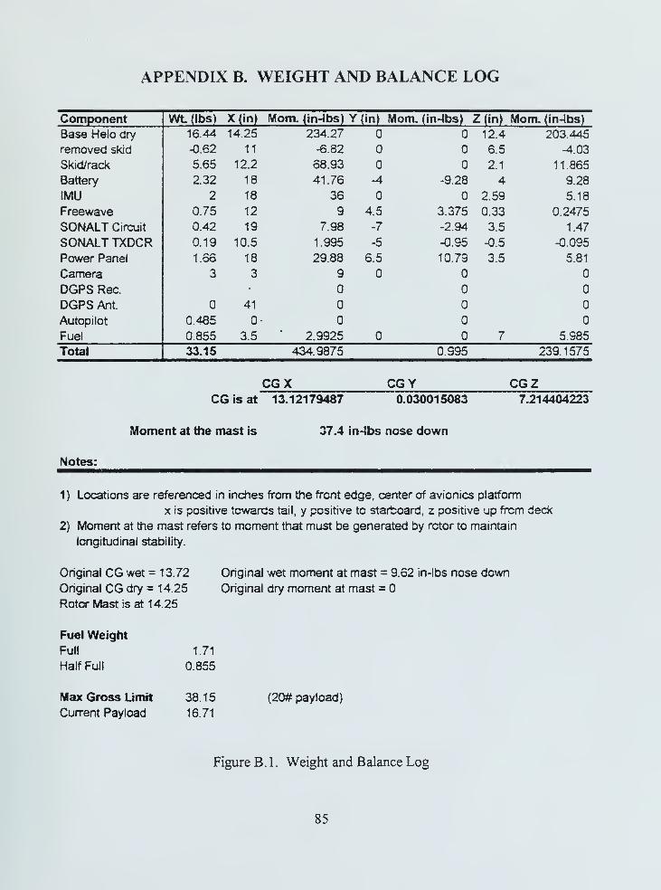
APPENDIX B. WEIGHT AND BALANCE LOG
Component Wt (lbs) X(in) Mom. (in-lbs) Y (in) Mom. (in-lbs) .Z(in) Mom. (in-lbs)
Base Helo dry 16.44 14.25 234.27 12.4 203.445
removed skid -0.62 11 -6.82 6.5 ^.03
Skid/rack 5.65 12.2 68.93 2.1 11.865
Battery 2.32 18 41.76 A -9.28 4 9.28
IMU 2 18 36 2.59 5.18
Freewave 0.75 12 9 4.5 3.375 0.33 0.2475
SONALT Circuit 0.42 19 7.98 -7 -2.94 3.5 1.47
SONALT TXDCR 0.19 10.5 1.995 -5 -0.95 -0.5 -0.095
Power Panel 1.66 18 29.88 6.5 10.79 3.5 5.81
Camera 3 3 9
DGPS Rec.
DGPS Ant. 41
Autopilot 0.485 0-
Fuel 0.855 3.5 2.9925 7 5.985
Total 33.15 434.9875 0.995 2391575
CGXCG is at 13.12179487
CGY0.030015083
CGZ7.214404223
Moment at the mast is 37.4 in-Jbs nose down
Notes:
1) Locations are referenced in inches from the front edge, center of avionics platform
x is positive towards tail, y positive to starboard, z positive up from deck
2) Moment at the mast refers to moment that must be generated by rotor to maintain
longitudinal stability.
Original CG wet = 13.72
Original CG dry = 14.25
Rotor Mast is at 14.25
Original wet moment at mast = 9.62 in-lbs nose down
Original dry moment at mast =
Fuel Weight
Full
Half Full
1.71
0.855
Max Gross Limit 38 1
5
Current Payload 16.71
(20# payload)
Figure B. 1 . Weight and Balance Log
85

86

APPENDIX C. AVIONICS SYSTEM WIRING DIAGRAMS
Figure C. 1 . SONALT Wiring Diagram Part One
87

Figure C.2. SONALT Wiring Diagram Part Two
88

WhiteTmI Point
D-
Red
T«« Point
SUckTesl Point
7>jV Battfrcy <y^>-
Up External{
Down Battery*
White- Red
IMU
Grey Ribbon Wires
i4' t l- i' wel 5
r C ia wel 1
10 — Channel 1
9 — Channel *
8 — Channel 3
7 — Channel 4
6 — Ground
CON10CJon*? strip on powei
converter support
«M flannel 3
K- *ei-/ iiywl *4-
DB9 Female EtlemaJ
CON12A J6
*- 11
— 9
— 5— 3
18-36V in 2<V out
wer ConnecBlack
tar
Power Gn i
Grey
Regulated '2tv
Rc37SIack
jate inqate out trltt_7.
Inland OCDC3SVIH 2«V OUT
ACOti H30S 2412
Red/Blacfc 6 '- I"
• 2»v
_L
IN
18-36V IN
ovovj?
12V
-SI
TRIM 3
• S<
XBT2
12V
Figure C.3. Avionics Power and Signal Distribution
89

90
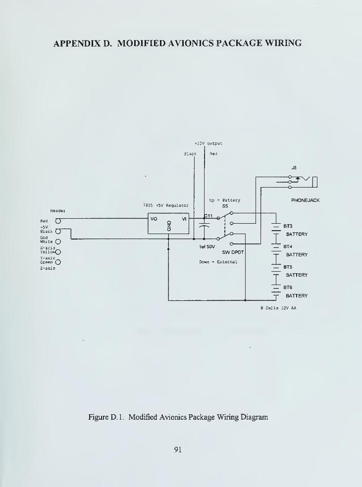
APPENDIX D. MODIFIED AVIONICS PACKAGE WIRING
Header
Red Q"+W —Black (JGnd _White OX-axisYellov<3
Y-axi>:Green QZ-axis
+ 12V output.
Black
7805 +5V Regulator
vo VI
Red
Up = Battery
SS
21L-&^
^°-1uf50V
w
SW DPDT
Down = External
J8
3^DPHONEJACK
"1
III
_ BT3
BATTERY
7 BT4
BATTERY
7 BT5
BATTERY
_ BT6
"y~ BATTERY
8 Cells 12V AA
Figure D. 1 . Modified Avionics Package Wiring Diagram
91

92

APPENDIX E. BLADE ANGLE VS. PULSE WIDTH DATA
Collective AOA vs. PWM
10 -
8-
6 -
a A
o2,
« 2 -
ac<01
I °-m 11
-2-
-4 -
-6 -
30
>yj
^>^
XI 1230 1330 1430 1530 1630^s. 170) 1830 1£
y = -0.020&
P2 -
^^^+ 33^^09 /ig
PWM
Figure E. 1 Collective Blade Angle vs. Throttle PWM
93

£1130
Lateral Cyclic AOA vs. PWM
12X1 13X 14X1 16X1
PWM
y = 00118x- 18.258
R^= 0.9981
17D0 18X1 1S0O
Figure E.2. Lateral Cyclic Blade Angle vs. Lateral Cyclic PWM
94
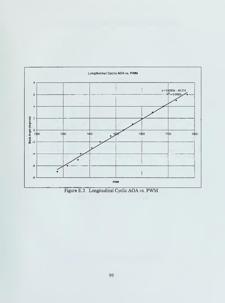
M 2
* o
12X1
a -2
Longitudinal Cyclic AOA vs. PWM
13X1 1430 16X1
PWM
y=0. D263x -40.274- 9953,
1730 1£X»
Figure E.3. Longitudinal Cyclic AOA vs. PWM
95

Tail Rotor AOA vs. PWM
30
20
10
£ r.o)
f. 12b0 13D0 14D0
-10
-20
-30
-40
15X1 630 1730 18X)
y = -0 0977x + ' 501^ -09^
1S30
Figure E.4. Tail Rotor AOA vs. PWM
96

APPENDIX F. REALSIM SUPERBLOCK DIAGRAMS
l-JUN-98
Discrete SuperBlock Sample Period Sample Skew Inputs Outputs Enable Signal
Command Tx 0.04 0. 45 16 Parent
&B2--*-
ha
C&n-0»nu.
iyCD™1-
a?m. i
0>nu-
ro111*-*""
TTtGD
TB
^~.
n ^„ — a fi-^
TO
r©—a>
t
rf-"
£>~
Figure F. 1 . PWM to Blade Angle Conversion Blocks
97

l-JUN-98
Discrete SuperBlock
A D IMUSample Period Sample Skew
0.04 . 0.
Inputs Outputs
20 4
Enable Signal
Parent
el_alpha_rad_all
Yl = S. 618-01 - 16.461 Li.
Y2 = -62.5*02 . 176.25
Y3 = -(11.905*03 - 33.81)
Y4- 7.7S2*04 - 26.977
En>tas_alt_el_all
Yl= 1.96*01 - 4.75
Y2= 1.98*02 - 4.82
Y3= 1.94*U3 - 4.79
Y4- 6.1263*04 0.33
Figure F.2. Acceleration and Altitude Voltage Conversion Superblocks
98

APPENDIX G. FLIGHT TEST DATA
6
~5h
0)4o£3
10 15 20 25 30 35
f529-1 Vertical Doublets
15 20Time (sec)
Figure G. 1. SONALT Altitude During Vertical Doublets, Top: filtered, Bottom: raw
99

a> 0.1
OOCO
XCD
-0.1
10 15 20Time (sec)
Figure G.2. Filtered Acceleration and Collective PWM Data During Vertical Doublets
100

4-
« 3o
<
1-
10 15 20 25 30 35
4-
*3
12<
1-
f529-2 Lateral Doublets
i i
L ft ...\ JUL...!
i
: / \
>T5. .. ,.A L
s
|\zv „
1
fL-,7 1pj -1(Y- /%i -va^j;
f *n V,
ii
i o"
10 15 20Time (sec)
25 30 35
Figure G.3. SONALT Altitude During Lateral Doublets; Top: filtered, Bottom: raw
101

o> 0.
CDOOco
CO
XCD
>>-0.
5 10 15 20 25 30 35Z I
1 1,1li
I
i
illI
1
i i
pf-ftyjtftmfi-Wffr1%fkfm«bkiAo i
ii
i i
10 15 20 25
10 15 20 25Time (sec)
30 35
35
Figure G.4. Filtered Acceleration and Lateral Cyclic PWM Data During Lateral Doublets
102

^2
10 15 20 25 30 35
f529-3 Longitudinal Doublets
15 20Time (sec)
Figure G.5. SONALT Altitude During Longitudinal Doublets;
Top: filtered, Bottom: raw
103

10 15 20Time (sec)
25 30
Figure G.6. Filtered Acceleration and Longitudinal Cyclic
PWM Data During Longitudinal Doublets
104

f529-4 Steps
15 20Time (sec)
Figure G.7. SONALT Altitude During Vertical Steps;
Top: filtered, Bottom: raw
105
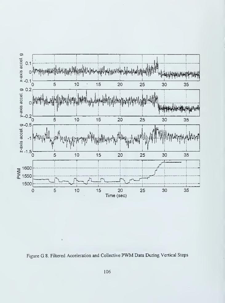
0)
8 0.11-
CO
.<2
XCO
-0.1
Hww#*^^
10 15 20Time (sec)
25 30
5 10 15 20 25 30 35
i i i r i i
1600
1550A. :n_
1500i i i ' i i i
35
Figure G.8. Filtered Acceleration and Collective PWM Data During Vertical Steps
106

f529-5 Vertical Doublets
15 20
Time (sec)
Figure G.9. SONALT Altitude During Vertical Doublets;
Top: filtered, Bottom: raw
107

"55
ooCD
XCO
I
N
5 10 15 20 25 30 35
-0.5
-1
-1.5
, i i i i i i i
2 i .
"ww i Ml'iiil
i * i y i i i i
1800
1600-
1400
10
10
15 20 25
15 20Time (sec)
25
30
30
35
35
Figure G.10. Filtered Acceleration and Collective PWM Data During Vertical Doublets
108

t=linspace(0,38.46,7692)
;
% This code filters altitude data from the loaded file and creates a
% plot of the filtered data against time above the original data.% 5/24/98 D.S. Greer
%load f2_523;alt=f(:,4);alt2=alt;for i=2 : size (alt)
if alt(i)<lif alt(i-l)>l
for j=i:i+25
alt2(j)=alt(i-l) + (alt(i+2 6)-alt(i-l) )/27*(j-i+l) ;
endend
endif i>8
alt2 (i)=mean(alt2 (i-8:i) )
;
end
endsubplot (2,1,1)plot (t,alt2, 'r' ) ;gridylabel (
' Altitude ( ft )
'
)
axis( [0,38,0,11]
)
subplot (2,1,2)plot (t,alt, 'b' ) ;gridylabel ( 'Altitude (ft)')xlabel ( "Time (sec) 1
)
axis ([0,38, 0,11]);
Figure G. 1 1 . MATLAB Script for Digitally Filtering SONALT Data
109

110

INITIAL DISTRIBUTION LIST
1
.
Defense Technical Information Center 2
8725 John J. Kingman Rd., STE 0944
Ft. Belvoir, Virginia 22060-6218
2. Dudley Knox Library 2
Naval Postgraduate School
411 DyerRd.
Monterey, California 93943-5101
3. Dr. Russ W. Duren 2
Department of Aeronautics and Astronautics, Code AA/DRNaval Postgraduate School
Monterey, California 93943-5101
4. Dr. Isaac I. Kaminer 1
Department of Aeronautics and Astronautics, Code AA/KANaval Postgraduate School
Monterey, California 93943-5101
5. Chairman 1
Department of Aeronautics and Astronautics, Code AANaval Postgraduate School
Monterey, California 93943-5101
6. Daniel S. Greer 2
1105 Leahy Rd.
Monterey, California 93940
111


10/99 22^7-20??^*I