
Prepared in cooperation with the Pennsylvania Department of Health and the Pennsylvania Department of Environmental Protection
Arsenic Concentrations, Related Environmental Factors, and the Predicted Probability of Elevated Arsenic in Groundwater in Pennsylvania
Scientific Investigations Report 2012–5257
U.S. Department of the InteriorU.S. Geological Survey

Cover: See figure 5 for an explanation of arsenic concentrations in groundwater.

Arsenic Concentrations, Related Environmental Factors, and the Predicted Probability of Elevated Arsenic in Groundwater in Pennsylvania
By Eliza L. Gross and Dennis J. Low
Prepared in cooperation with the Pennsylvania Department of Health and the Pennsylvania Department of Environmental Protection
Scientific Investigations Report 2012–5257
U.S. Department of the InteriorU.S. Geological Survey

U.S. Department of the InteriorKEN SALAZAR, Secretary
U.S. Geological SurveySuzette M. Kimball, Acting Director
U.S. Geological Survey, Reston, Virginia: 2013
For more information on the USGS—the Federal source for science about the Earth, its natural and living resources, natural hazards, and the environment, visit http://www.usgs.gov or call 1–888–ASK–USGS.
For an overview of USGS information products, including maps, imagery, and publications, visit http://www.usgs.gov/pubprod
To order this and other USGS information products, visit http://store.usgs.gov
Any use of trade, product, or firm names is for descriptive purposes only and does not imply endorsement by the U.S. Government.
Although this report is in the public domain, permission must be secured from the individual copyright owners to reproduce any copyrighted materials contained within this report.
Suggested citation:Gross, E.L., Low, D.J., 2013, Arsenic concentrations, related environmental factors, and the predicted probability of elevated arsenic in groundwater in Pennsylvania: U.S. Geological Survey Scientific Investigations Report 2012–5257, 46 p.

iii
Acknowledgments
This work was performed under the collaborative sub-grant 5U38EH000191-4 from the Pennsylvania Environmental Public Health Tracking Program (PA EPHT) of the Pennsylvania Department of Health, Bureau of Epidemiology, and the Pennsylvania Department of Environmental Protection.
Contents
Abstract ...........................................................................................................................................................1Introduction.....................................................................................................................................................1
Purpose and Scope ..............................................................................................................................2Background on Arsenic Occurrence ................................................................................................2Description of Study Area ...................................................................................................................3Previous Studies ...................................................................................................................................5
Methods of Investigation ..............................................................................................................................6Groundwater-Quality Data ..................................................................................................................6Spatial Data............................................................................................................................................6
Anthropogenic Factors ...............................................................................................................8Natural Factors.............................................................................................................................8
Statistical Methods.............................................................................................................................11Probability Maps ................................................................................................................................13
Arsenic Concentrations and Related Factors .........................................................................................13Arsenic Concentrations .....................................................................................................................13Significance of Groundwater-Quality Properties Related to Arsenic ........................................15Redox Conditions ................................................................................................................................16
Predicted Probability of Elevated Arsenic Concentrations in Groundwater ....................................18Statewide .............................................................................................................................................19Glacial Aquifer System.......................................................................................................................21Gettysburg Basin.................................................................................................................................23Newark Basin ......................................................................................................................................25
Limitations and Uses of Arsenic Models and Probability Maps ..........................................................27Summary and Conclusions .........................................................................................................................29References Cited..........................................................................................................................................30Appendix 1. Summary of statewide and regional anthropogenic and natural factors used
as explanatory variables in logistic regression models for elevated arsenic concentrations in groundwater in Pennsylvania and number of sample records ..............35
Appendix 2. Summary of arsenic concentrations in groundwater (1969–2007) for the 193 geologic units in Pennsylvania with major aquifer type and primary lithology ...................39
Appendix 3. Results of univariate logistic regression analyses with logistic regression standardized coefficients and individual p-values of independent variables related to the detection of elevated concentrations of arsenic in groundwater samples collected statewide and in three regions in Pennsylvania .....................................................44

iv
Figures 1. Map showing physiographic provinces and sections, major aquifer types, and the
extent of the Wisconsin glaciation in Pennsylvania ...............................................................4 2. Map showing intrastate regions modeled in Pennsylvania ..................................................7 3. Map showing location of sampling sites and associated reported arsenic concen-
trations in groundwater in Pennsylvania, 1969–2007 ............................................................14 4. Graphs showing percentage of observed detections of elevated arsenic concen-
trations in relation to the average predicted probability of detecting elevated arsenic concentrations in groundwater statewide and in three regions in Pennsylvania ...........21
5. Map showing areas with predicted probability that arsenic concentrations in ground-water in surficial and bedrock aquifers statewide in Pennsylvania will be greater than or equal to 4.0 micrograms per liter and sampling sites with associated Pearson residual values showing predictive error for measured arsenic concentrations ...........22
6. Map showing areas with predicted probability that arsenic concentrations in ground-water in the glacial aquifer system in Pennsylvania will be greater than or equal to 4.0 micrograms per liter and sampling sites with associated Pearson residual values showing predictive error for measured arsenic concentrations in wells .........................24
7. Map showing areas with predicted probability that arsenic concentrations in ground-water in the Gettysburg Basin in Pennsylvania will be greater than or equal to 4.0 micrograms per liter and sampling sites with associated Pearson residual values showing predictive error for measured arsenic concentrations ...........................26
8. Map showing areas with predicted probability that arsenic concentrations in ground-water in the Newark Basin in Pennsylvania will be greater than or equal to 4.0 micro-grams per liter and sampling sites with associated Pearson residual values showing predictive error for measured arsenic concentrations in wells .........................28
Tables 1. Summary of arsenic concentrations in groundwater (1969–2007) for the four major
aquifer types in Pennsylvania .....................................................................................................9 2. Summary of arsenic concentrations in groundwater (1969–2007) for the six physio-
graphic provinces in Pennsylvania ..........................................................................................15 3. Spearman’s rho correlations for the 17 groundwater-quality constituents that have
the best correlations with arsenic in groundwater in Pennsylvania and major aquifer types ................................................................................................................................16
4. Redox-pH matrix showing the frequency of arsenic in 5,023 groundwater samples collected statewide in Pennsylvania, by redox classification and range of arsenic concentrations. ..........................................................................................................................17
5. Summary of statistics for statewide and regional logistic regression models predicting the probability of arsenic exceeding 4.0 micrograms per liter statewide and in three regions in Pennsylvania .............................................................................................................20

v
Conversion Factors
SI to Inch/Pound
Multiply By To obtain
Length
centimeter (cm) 0.3937 inch (in)
millimeter (mm) 0.03937 inch (in)
meter (m) 3.281 foot (ft)
kilometer (km) 0.6214 mile (mi)
Area
square centimeter (cm2) 0.001076 square foot (ft2)
square meter (m2) 10.76 square foot (ft2)
square centimeter (cm2) 0.1550 square inch (ft2)
square kilometer (km2) 0.3861 square mile (mi2)
Volume
liter (L) 0.2642 gallon (gal)
Mass
gram (g) 0.03527 ounce, avoirdupois (oz)
Temperature in degrees Celsius (°C) may be converted to degrees Fahrenheit (°F) as follows:
°F=(1.8×°C)+32
Temperature in degrees Fahrenheit (°F) may be converted to degrees Celsius (°C) as follows:
°C=(°F-32)/1.8
Vertical coordinate information is referenced to the North American Vertical Datum of 1988 (NAVD 88).
Horizontal coordinate information is referenced to the North American Datum of 1983 (NAD 83).
Elevation, as used in this report, refers to distance above the vertical datum.
Specific conductance is given in microsiemens per centimeter at 25 degrees Celsius (µS/cm at 25 °C).
Concentrations of chemical constituents in water are given either in milligrams per liter (mg/L) or micrograms per liter (µg/L).


Arsenic Concentrations, Related Environmental Factors, and the Predicted Probability of Elevated Arsenic in Groundwater in Pennsylvania
By Eliza L. Gross and Dennis J. Low
AbstractAnalytical results for arsenic in water samples from
5,023 wells obtained during 1969–2007 across Pennsylvania were compiled and related to other associated groundwater-quality and environmental factors and used to predict the prob-ability of elevated arsenic concentrations, defined as greater than or equal to 4.0 micrograms per liter (µg/L), in ground-water. Arsenic concentrations of 4.0 µg/L or greater (elevated concentrations) were detected in 18 percent of samples across Pennsylvania; 8 percent of samples had concentrations that equaled or exceeded the U.S. Environmental Protection Agen-cy’s drinking-water maximum contaminant level of 10.0 µg/L. The highest arsenic concentration was 490.0 µg/L.
Comparison of arsenic concentrations in Pennsylvania groundwater by physiographic province indicates that the Cen-tral Lowland physiographic province had the highest median arsenic concentration (4.5 µg/L) and the highest percentage of sample records with arsenic concentrations greater than or equal to 4.0 µg/L (59 percent) and greater than or equal to 10.0 µg/L (43 percent). Evaluation of four major aquifer types (carbonate, crystalline, siliciclastic, and surficial) in Pennsyl-vania showed that all types had median arsenic concentra-tions less than 4.0 µg/L, and the highest arsenic concentration (490.0 µg/L) was in a siliciclastic aquifer. The siliciclastic and surficial aquifers had the highest percentage of sample records with arsenic concentrations greater than or equal to 4.0 µg/L and 10.0 µg/L. Elevated arsenic concentrations were associ-ated with low pH (less than or equal to 4.0), high pH (greater than or equal to 8.0), or reducing conditions. For waters clas-sified as anoxic (405 samples), 20 percent of sampled wells contained water with elevated concentrations of arsenic; for waters classified as oxic (1,530 samples) only 10 percent of sampled wells contained water with elevated arsenic concen-trations. Nevertheless, regardless of the reduction-oxidation classification, 54 percent of samples with low pH (13 of 24 samples) and 25 percent of samples with high pH (57 of 230 samples) had elevated arsenic concentrations.
Arsenic concentrations in groundwater in Pennsylva-nia were correlated with concentrations of several chemical constituents or properties, including (1) constituents associated
with redox processes, (2) constituents that may have a similar origin or be mobilized under similar chemical conditions as arsenic, and (3) anions or oxyanions that have similar sorption behavior or compete for sorption sites on iron oxides.
Logistic regression models were created to predict and map the probability of elevated arsenic concentrations in groundwater statewide in Pennsylvania and in three intrastate regions to further improve predictions for those three regions (glacial aquifer system, Gettysburg Basin, Newark Basin). Although the Pennsylvania and regional predictive models retained some different variables, they have common charac-teristics that can be grouped by (1) geologic and soils variables describing arsenic sources and mobilizers, (2) geochemical variables describing the geochemical environment of the groundwater, and (3) locally specific variables that are unique to each of the three regions studied and not applicable to state-wide analysis. Maps of Pennsylvania and the three intrastate regions were produced that illustrate that areas most at risk are those with geology and soils capable of functioning as an arsenic source or mobilizer and geochemical groundwater conditions able to facilitate redox reactions. The models have limitations because they may not characterize areas that have localized controls on arsenic mobility. The probability maps associated with this report are intended for regional-scale use and may not be accurate for use at the field scale or when considering individual wells.
IntroductionIn many areas worldwide, including Pennsylvania, drink-
ing water is the primary route of human exposure to arsenic (Hopenhayn, 2006). Arsenic data are sparse for groundwater because statewide testing of private wells to determine where concentrations exceed the health-based maximum contami-nant level (MCL) of 10.0 micrograms per liter (µg/L) for drinking water, established in 2001 by the U.S. Environmen-tal Protection Agency (USEPA), is not required throughout Pennsylvania (U.S. Environmental Protection Agency, 2006). Domestic wells used for private water supplies in Pennsylva-nia are not required to be routinely tested for arsenic and other

2 Arsenic Concentrations, Environmental Factors, and the Probability of Elevated Arsenic in Groundwater in Pa.
contaminants, so homeowners may not know whether their well water has arsenic concentrations greater than the MCL.
Arsenic is a known carcinogen and consumption of arsenic in drinking water has been linked to multiple health problems, including bladder, lung, prostate, and skin cancers; cardiovascular disease; diabetes; and neurological disfunc-tion (National Research Council, 1999, 2001; Hopenhayn, 2006; Chen and others, 2007; Benbrahim-Tallaa and Waalkes, 2007; Lin and others, 2008). Arsenic is also a potent endo-crine disruptor that can cause problems with reproduction and embryotic development (Davey and others, 2007). In 2001, the USEPA decreased the drinking water MCL from 50.0 to 10.0 µg/L in recognition of the health risks associated with arsenic (U.S. Environmental Protection Agency, 2006). Although the USEPA regulates only public water-supply sys-tems, the MCL has general applicability for the consumption of drinking water from private domestic wells.
Arsenic concentrations in Pennsylvania groundwater are difficult to predict on a well-by-well basis because (1) there is considerable local- and regional-scale spatial variability in groundwater quality and (2) arsenic has multiple anthro-pogenic and natural sources. However, the risk of elevated arsenic concentrations in groundwater is greater in some areas of Pennsylvania than in others (Low and Galeone, 2006). If areas with increased probability for elevated arsenic concen-trations could be identified, health monitoring, water-quality monitoring, and educational programs could then be directed where the need is greatest. To address these concerns, the U.S. Geological Survey, in cooperation with the Pennsylva-nia Department of Health and Pennsylvania Department of Environmental Protection, undertook a study in 2010 to deter-mine areas in Pennsylvania that have increased probability of elevated arsenic concentrations in groundwater using available data describing arsenic concentrations, groundwater chemistry, geology, and other factors.
Purpose and Scope
This report (1) documents arsenic concentrations in groundwater samples collected in Pennsylvania during 1969–2007, (2) describes the relation between arsenic concen-trations and reduction-oxidation (redox) conditions and other groundwater-quality variables, and (3) documents the devel-opment of logistic regression models to represent the spatial relation between arsenic concentrations in groundwater and anthropogenic and natural factors. The models were developed using existing and constructed geographic information system (GIS) data for Pennsylvania and three intrastate regions (glacial aquifer system, Gettysburg Basin, and Newark Basin). Resulting model coefficients for selected spatial variables were used to produce maps displaying the predicted probabil-ity of elevated arsenic concentrations (greater than or equal to 4.0 µg/L) throughout the State and the selected intrastate regions.
Background on Arsenic Occurrence
Arsenic is a naturally occurring trace element in rock, soil, plants, and the aquatic environment. A recent review of occurrence of arsenic in natural waters describes some principal sources and mechanisms of arsenic mobility in groundwater (Smedley and Kinniburgh, 2002). Concentrations of arsenic in groundwater vary greatly owing to the uneven distribution of source materials and dynamic geochemical controls on aqueous arsenic mobility. Although arsenic can be introduced to the environment from anthropogenic sources (such as contaminant releases from industrial facilities or usage as a pesticide for agriculture), it commonly is present as a trace component in naturally occurring minerals, such as sulfides (pyrite), hydrous metal oxides (iron oxides), coal, ironstones, clays, phosphates, silicates, and carbonates. Pyrite and iron oxides are important sources of elevated arsenic in groundwater because they are abundant in aquifers, leading to their dissemination throughout the aquifer matrix or accu-mulation in fractures, joints, or bedding planes (Smedley and Kinniburgh, 2002).
Arsenic, present as arsenic minerals or as a trace compo-nent in other naturally occurring minerals in the soil and aqui-fers, can be released to or removed from the groundwater as a result of oxidation and reduction, dissolution and precipitation, and surface complexation (sorption) reactions on mineral sur-faces. Arsenian pyrite [Fe(S,As)2], arsenopyrite (FeAsS), and (or) other unspecified sulfide minerals in bedrock and surficial sediments are common parent sources for naturally occurring arsenic in the environment (Foster and others, 2003). Substitu-tion of arsenic for sulfur in sulfide minerals can increase their susceptibility to weathering and dissolution when exposed to oxidants (Savage and others, 2000). Arsenic released to solu-tion by sulfide oxidation commonly has a valence state of V or III and forms the protonated oxyanion complexes, arsenate (HnAsO4
n-3) or arsenite (HnAsO3n-3), respectively (Welch and
others, 2000; Smedley and Kinniburgh, 2002; Stollenwerk, 2003). Arsenite is considered the more toxic of the two major oxyanion forms.
Arsenate [As(V)] predominates in oxic groundwaters, whereas arsenite [As(III)] predominates in reducing sulfidic and methanic groundwaters (Welch and others, 2000; Smed-ley and Kinniburgh, 2002; Stollenwerk, 2003). In strongly reducing waters that are near saturation with sulfide minerals, arsenic sulfide complexes and minerals may form. Mueller and others (2001) noted that the prevalence of arsenite was correlated with low concentrations of dissolved oxygen that reflect strongly reducing conditions (dissolved oxygen less than 0.1 milligrams per liter (mg/L)); arsenate was associ-ated with oxidizing conditions (dissolved oxygen greater than 8 mg/L). The conversion of As(III) to As(V) in oxic waters may be relatively slow and can be measured in years (Eary and Schramke, 1990) with pH, ferric iron, manganese, and bacteria strongly affecting the rate of oxidation. The reduction of As(V) to As(III) under anaerobic conditions is generally much faster than the oxidation of As(III) to As(V).

Introduction 3
In groundwater systems, arsenate and arsenite oxy-anions commonly form surface complexes (adsorption) on iron oxides and other mineral surfaces (Stollenwerk, 2003). Although As(V) and As(III) adsorb over a wide pH range, As(V) is extensively adsorbed at low pH values and desorbs at alkaline pH; As(III) adsorption increases with pH and peaks at about pH 8 or 9 (Stollenwerk, 2003). In addition to iron oxides, a wide variety of minerals including aluminum oxides and oxyhydroxides, manganese oxides, silica, clays, and car-bonates may sorb arsenic, and dissolved organic compounds, phosphate, and other dissolved ions can influence the adsorp-tion of arsenic.
Mobilization of adsorbed arsenic may occur through desorption or dissolution of the host mineral. Arsenic associ-ated with iron oxides tends to be weakly bound on surface sites (adsorbed) and can be released to the groundwater by desorption or by dissolution of the iron oxides (Matisoff and others, 1982; Ayotte and others, 1998; Welch and others, 2000; Smedley and Kinniburgh, 2002; Stollenwerk, 2003; Thomas and others, 2008). Changes in pH and (or) redox conditions can result in the release of arsenic from minerals. Increases in pH can lead to the desorption of arsenate and arsenite. The development of reducing conditions can lead to the reductive dissolution of iron oxides and (or) the reduction of arsenate to arsenite and the consequent desorption of arsenite (reductive desorption) (Stollenwerk, 2003; Thomas, 2007). In general, fine-grained sediments tend to have higher arsenic concentra-tions than coarse-grained sediments because smaller-sized particles and (or) those with complex shapes have a higher surface-area-to-volume ratio and a more reactive surface area than larger, simply shaped particles (Parks, 1990). The density of sorption sites and potential exposure to reactive waters generally increase with the mineral surface area.
Arsenic concentrations in groundwater may increase (accumulate) with the age of the water. Thomas (2007) reported that arsenic concentrations of 10.0 µg/L or greater were found more frequently in old waters (recharged before 1953) as compared to younger waters (recharged since 1953). Geologic units that have high yields of water are, in general, highly permeable and transmissive, exhibit rapid recharge, and, as a result, consist of relatively young water. This young water will typically be predominantly oxic. In general, water in shallow wells is more likely to be affected by anthropogenic contaminants than water in deeper wells; however, excep-tions are numerous because of complexities of groundwater flowpaths.
Description of Study Area
Pennsylvania is a physiographically, geologically, and hydrologically diverse State that covers about 139,859 square kilometers (54,000 square miles). Pennsylvania includes parts of six physiographic provinces, which are subdivided into 20 physiographic sections—(1) Appalachian Plateaus (Allegheny Mountain, Allegheny Plateau, Clarion Plateau,
Deep Valleys, Glaciated High Plateau, Glaciated Low Plateau, High Plateau, Glaciated Pocono Plateau, Northwestern Glaci-ated Plateau, Pittsburgh Low Plateau, Waynesburg Hills), (2) Atlantic Coastal Plain (Lowland and Intermediate Upland), (3) Central Lowland (Eastern Lake), (4) New England (Reading Prong), (5) Piedmont (Gettysburg-Newark Lowland, Pied-mont Lowland, Piedmont Upland), and (6) Ridge and Val-ley (Appalachian Mountain, Great Valley, South Mountain) (Fenneman and Johnson, 1946; Berg and others, 1989) (fig. 1). Land-surface elevations range from sea level (North American Verical Datum of 1988; NAVD 88) (Atlantic Coastal Plain) to 978 meters (3,210 feet) above NAVD 88 (Appalachian Plateaus).
The topography of the Appalachian Plateaus Phys-iographic Province (hereafter province) varies from deep valleys to glaciated high plateaus with dominant rock types of sandstone, siltstone, and shale and abundant bituminous coal in places. The geologic structure of the Appalachian Plateaus province is complex, varying from horizontal beds to large-amplitude open folds. The Atlantic Coastal Plain province has little relief and consists of unconsolidated sand, gravel, and clay that overlie metamorphic rocks. The Central Lowland province also has little relief with considerable sand and gravel and beach deposits in the Lake Erie area. The New England province includes the steep hills and rounded ridges of the Reading Prong physiographic section (hereafter sec-tion), which consists of highly metamorphosed granitic rocks and quartzite. The Piedmont province topography consists of broad, rolling lowlands, narrow valleys, and broad, flat-topped hills. Shale, siltstone, sandstone, and diabase dominate the Gettysburg-Newark Lowland section of the Piedmont prov-ince; limestone and dolomite are common in the Piedmont Lowland section. The Piedmont Upland section is dominated by schist, gneiss and quartzite. The geologic structures of the Piedmont province are variable, ranging from half-grabens in the Gettysburg-Newark Lowland section to complex folds and faults elsewhere in the province. The topography of the Ridge and Valley province ranges from narrow to broad valleys with steep uplands or linear ridge and mountain tops. Dominant rock types in the Ridge and Valley province are sandstone, siltstone, and shale, except in the Great Valley section and val-leys of the Appalachian Mountain section, which are underlain predominantly by limestone and dolomite rocks. The geologic structure within the Ridge and Valley province is complex with many folds, faults, thrust sheets, nappes, and a major anticlinorium with second- and third-order folds.
Pennsylvania has a complex geological history, which results in many different rock types within the State, with the Pennsylvania Geological Survey recognizing almost 200 different geologic formations or members (Berg and others, 1980; Pennsylvania Geological Survey, 2001). Despite the geologic diversity within the State, the groundwater system in Pennsylvania has been characterized as being representative of four major aquifer types—(1) carbonate bedrock (limestone and dolomite), (2) crystalline bedrock (igneous and meta-morphic rocks), (3) siliciclastic bedrock (sandstone, siltstone,

4 Arsenic Concentrations, Environmental Factors, and the Probability of Elevated Arsenic in Groundwater in Pa.
Appa
lach
ian
Mou
ntai
n
Deep
Val
leys
Pitts
burg
h Lo
w P
late
au
Glac
iate
d Lo
w P
late
au
Grea
t Val
ley
High
Pla
teau
Alle
ghen
y M
ount
ain
Pied
mon
t Upl
and
Getty
sbur
g-N
ewar
k Lo
wla
nd
Clar
ion
Plat
eau
Nor
thw
este
rn
Glac
iate
d Pl
atea
u
Way
nesb
urg
Hill
s
Allegheny P
lateau
Pied
mon
t Lo
wla
nd
Glac
iate
d Po
cono
Pl
atea
u
South Mountain
Glac
iate
d Hi
gh P
late
au
Lake
Eri
e
Base
from
U.S
. Bur
eau
of th
e Ce
nsus
dig
ital d
ata,
199
0b 1
:100
,000
Al
bers
Equ
al-A
rea
Coni
c pr
ojec
tion:
Sta
ndar
d Pa
ralle
ls 4
0° N
and
42
° N
, Cen
tral M
erid
ian
-78°
W, L
atitu
de o
f Orig
in 3
9°
Phys
iogr
aphi
c pr
ovin
ces
and
sect
ions
mod
ified
from
Pen
nsyl
vani
a Ge
olog
ical
Sur
vey,
19
98 M
ajor
aqu
ifer t
ypes
from
Lin
dsey
and
Bic
kfor
d, 1
999;
Pen
nsyl
vani
a Ge
olog
ical
Su
rvey
, 200
1; S
olle
r & P
acka
rd, 1
998
Exte
nt o
f Wis
cons
in g
laci
atio
n fro
m P
enns
yl-
vani
a Ge
olog
ical
Sur
vey,
199
5
NE
W J
ER
SEY
MA
RY
LA
ND
WE
ST V
IRG
INIA
OH
IO
NE
W Y
OR
K
ATLA
NTI
C CO
ASTA
L PL
AIN
PR
OVIN
CELo
wla
nd a
nd
Inte
rmed
iate
Up
land
NEW
EN
GLAN
DPR
OVIN
CERe
adin
g Pr
ong
RIDG
E AN
D VA
LLEY
PRO
VIN
CEPI
EDM
ONT
PROV
INCE
CEN
TRAL
LOW
LAN
D PR
OVIN
CEEa
ster
n La
ke
APPA
LACH
IAN
PLA
TEAU
S PR
OVIN
CE
EXPL
AN
ATI
ON
Phys
iogr
aphi
c se
ctio
ns
Maj
or a
quife
r typ
es
Carb
onat
e
Crys
talli
ne
Silic
icla
stic
Surfi
cial
Phys
iogr
aphi
c pr
ovin
ces
Exte
nt o
f Wis
cons
in g
laci
atio
n
DELAWARE
75°0
0’76
°00’
77°0
0’79
°00’
80°0
0’78
°00’
42°
00’
41°
00’
40°
00’
39°
00’
025
MIL
ES12
.5
025
KIL
OMET
ERS
12.5
Figu
re 1
. Ph
ysio
grap
hic
prov
ince
s an
d se
ctio
ns, m
ajor
aqu
ifer t
ypes
, and
the
exte
nt o
f the
Wis
cons
in g
laci
atio
n in
Pen
nsyl
vani
a.

Introduction 5
conglomerate, and shale), and (4) surficial (fig. 1) (Lindsey and Bickford, 1999; Pennsylvania Geological Survey, 2001; Soller and Packard, 1998). Surficial aquifers consist of unconsolidated material (sand and gravel) overlying bed-rock aquifers in depths sufficient to serve as an aquifer, such as glacial outwash, alluvium, and beach deposits. Surficial aquifers shown in figure 1 consist of mapped areas of the State where surficial materials consist of coarse-grained sediment, and these were designated as surficial aquifers for this report. Despite this designation, it is still possible for wells located in other areas of the State within the extent of the Wisconsin glaciation (fig. 1) to be completed in glacial materials.
Carbonate bedrock aquifers are located in some valleys of the Pittsburgh Low Plateau section of the Appalachian Plateaus province, valleys of the Ridge and Valley province, and the Piedmont Lowland section of the Piedmont prov-ince. Crystalline bedrock aquifers make up the New England province, the Piedmont Upland section and diabase intrusions of the Gettysburg-Newark Lowland section of the Piedmont province, and South Mountain section of the Ridge and Valley province. The Central Lowland and Atlantic Coastal Plain provinces are predominantly composed of surficial aquifers resulting from beach deposits from Lake Erie and the Atlantic Ocean. Siliciclastic bedrock aquifers can be found throughout the rest of the State and are most prominent in the Appalachian Plateaus province, Gettysburg-Newark Lowland section of the Piedmont province, and the Ridge and Valley province. Surficial deposits are also mostly in the Northwestern Gla-ciated Plateau and Glaciated Low Plateau sections of the Appalachian Plateaus province and are within the extent of the Wisconsin glaciation. Some surficial deposits also extend into the Appalachian Mountain section of the Ridge and Valley province and the Pittsburgh Low Plateau section of the Appa-lachian Plateaus province.
Temperature and precipitation vary across the State according to geography and topography. The average annual temperature is 11 degrees Celsius (ºC) (52 degrees Fahrenheit) in southern Pennsylvania and 8 ºC (46 degrees Fahrenheit) in the northern part of the State. The warmest areas correspond to the Atlantic Coastal Plain and Piedmont provinces. Progres-sive cooling occurs in the higher land-surface elevations of the Ridge and Valley province, and the Appalachian Plateaus province is the coolest area of the State (Cuff and others, 1989). Heat and moisture circulate through the State from the south to the southeast, whereas most of the precipitation-pro-ducing weather fronts move from west to east. Precipitation increases from 102 centimeters (cm) (40 inches) at the western border of Pennsylvania to a maximum of 130 cm (51 inches) near the highest land-surface elevations of the Appalachian Plateaus province. The decreasing land-surface elevations in the Ridge and Valley province create rain shadow effects that reduce the average annual precipitation to 97 cm (38 inches). The eastern part of Pennsylvania is strongly affected by airflows coming directly off the Atlantic Ocean, and this contributes to the higher average annual precipitation of 102 to
112 cm (40 to 44 inches), despite the lower land-surface eleva-tion (Cuff and others, 1989).
Land use is primarily forested (65 percent) followed by agricultural (27 percent) (Nakagaki and others, 2007). For-ested is the dominant land use in the north-central, northeast, and rugged mountain slopes. Agricultural land use predomi-nates in the valleys of the Ridge and Valley province and much of the Piedmont province. Urban (6 percent) land use is dominant in and around Pennsylvania’s major cities, espe-cially those cities with populations greater than 40,000 (U.S. Bureau of the Census, 2010), of which most are located in the Piedmont and Ridge and Valley provinces.
Previous Studies
Arsenic concentrations in groundwater of Pennsylvania have been documented by a number of previous studies, typi-cally a county-scale or regional-scale study. Cravotta (2008) reports that arsenic concentrations in groundwater discharged to 140 abandoned coal mines in the bituminous and anthra-cite coalfields of Pennsylvania ranged from less than 0.03 to 64.0 µg/L. Arsenic concentrations were positively correlated with pH, chloride, bromide, and iodide and inversely corre-lated with dissolved oxygen and redox potential, indicating the potential for arsenic mobilization by desorption or reduction processes, possibly because of interactions with deep, saline groundwater.
Williams and others (1998), who studied the glaciated valleys of Bradford, Potter, and Tioga Counties in Pennsylva-nia, found a correlation between arsenic and older (recharged before 1953) or briny water and found that arsenic concentra-tions varied by primary aquifer. Buckwalter and Moore (2007) concentrated their efforts in Warren County, which is also in a glaciated region of Pennsylvania, where almost one-third of the collected samples contained arsenic concentrations that exceeded the MCL of 10.0 µg/L; the maximum was 490.0 µg/L. They also documented that arsenic concentrations exhibited seasonal fluctuations and that arsenic concentrations varied widely, even between adjacent (less than a 76-meter (250-foot) distance) wells. Low and Galeone (2006) collected groundwater samples for analysis for total arsenic in the glaci-ated region of Pennsylvania within eight counties and found that arsenic concentrations varied greatly over short distances but did not appear to be related to well depth. Thomas (2007) studied the association of arsenic with redox conditions in the glacial aquifer system of the northern United States, which includes the glaciated portion of Pennsylvania and concluded that elevated arsenic concentrations are more commonly detected in older, anoxic groundwaters (recharged before 1953) and that arsenic correlated strongly with constituents linked to redox processes and anions or oxyanions that sorb to iron oxides.
Peters and Burkert (2008) examined groundwater-quality data from over 18,000 wells in the Newark Basin of Penn-sylvania. They found that variations in pH were strongly correlated with arsenic concentrations, with the highest

6 Arsenic Concentrations, Environmental Factors, and the Probability of Elevated Arsenic in Groundwater in Pa.
concentrations of arsenic associated with pH values greater than 6.4. They concluded that the original source of arsenic in the study area was most likely black and gray shales contain-ing arsenian pyrite and that groundwater concentrations of arsenic are most likely controlled by adsorption/desorption reaction with iron oxides in red mudstone aquifer materials. Senior and Sloto (2006) studied the Newark Basin, sampling 58 wells within the study area to identify areas of elevated arsenic concentrations and characterize the geochemical envi-ronment associated with elevated concentrations of arsenic and various constituents. They found that arsenic correlated most strongly and positively with pH, boron, and molybde-num; correlated positively with selenium, uranium, nickel, lithium, fluoride, and strontium; and correlated negatively with total organic carbon, copper, and dissolved oxygen. They concluded that arsenic concentrations may be controlled partly by pH affecting adsorption of arsenate and that the correlation of arsenic with the presence of many trace elements indicates similar geochemical controls and (or) distribution in aquifer materials in the Newark Basin.
Methods of InvestigationGroundwater-quality data from 1969 to 2007 were
obtained by the USGS from local, county, private, State, and Federal electronic databases. Spatial data consist of variables representing anthropogenic factors (such as land use and contamination sites) and natural factors (such as geology and climate) (appendix 1). Datasets for most factors were avail-able in geographic information system (GIS) format from various sources, but additional GIS datasets were developed specifically for use as explanatory variables during statisti-cal modeling. Some datasets listed in appendix 1 were not available statewide or pertinent to statewide analysis, so these datasets were only populated for selected intrastate regions (glacial aquifer system, Gettysburg Basin, Newark Basin) (fig. 2). Also, differences in the extent of explanatory variable data coverage caused different explanatory variables to have a different number of sample records associated with them. For example, a total of 5,023 sample records were available statewide, but appendix 1 shows 5,021 sample records avail-able statewide for all of the soil characterization variables and 5,011 sample records available statewide for two of the groundwater geochemistry variables. These differences in data availability were due to the slightly different extents associ-ated with the explanatory datasets, which caused these datasets to have slightly different coverage across Pennsylvania.
Groundwater-Quality Data
A database consisting of 5,023 groundwater records with reported values for arsenic and various associated field and laboratory measured constituents was created (Low and Chichester, 2006; Low and others, 2008). More than 25,000
groundwater-quality data records were examined initially. This number was reduced to create datasets containing values for arsenic (total and (or) dissolved, 12,781), pH (7,876), and spe-cific conductance (5,931). The pH and specific conductance datasets were used to create explanatory spatial variables, and these datasets include data from areas where arsenic data are not necessarily available. The arsenic dataset of 12,781 was further reduced to 5,023 groundwater records by restricting values to one composite sample per well using three methods: (1) samples with reported censored arsenic data with detection levels greater than 4.0 µg/L were removed from the database; (2) duplicate sites and (or) samples were removed through verification of local well numbers, site identifiers, geo-graphical coordinates (latitude and longitude) within the State boundary, and sample date; and (3) for sites that were sampled repeatedly, data from the analysis that was associated with the highest arsenic concentration were retained. If the arsenic concentrations were identical, then data from the most recent analysis were retained.
Groundwater-quality data associated with the arsenic dataset of 5,023 groundwater records were handled in the following manner: (1) values with remark values coded as “estimated” were assumed to represent actual values; (2) total and dissolved constituent samples were not differentiated in regards to any statistical or chemical analyses, but if total and dissolved values were reported for the same sample, the dissolved value was retained; and (3) field measurements (pH, specific conductance) had precedence over laboratory results. Estimated dissolved solids represents the maximum reported value for residue on evaporation at 105 ºC, residue dried at 180 °C, sum of dissolved constituents, or total dissolved solids. Although water use varied (commercial, monitor, industrial, public) no differentiation or statistical analysis was performed to distinguish among industrial, public, private, or other uses of water.
Groundwater-quality data associated with the arse-nic dataset of 5,023 groundwater records compiled for this investigation include up to 53 additional groundwater-quality constituents. These data were reduced to 31 groundwater-quality constituents for statistical analysis because of limited availability of data and differences in data quality among the records analyzed. Samples were analyzed at the USGS National Water Quality Laboratory, the Pennsylvania Depart-ment of Environmental Protection Laboratory, Pennsylvania Department of Agriculture, and Pennsylvania State University, as well as a number of private laboratories (Low and Chiches-ter, 2006; Low and others, 2008). As a result, the groundwater-quality data represent multiple project designs and goals, site and well selection criteria, as well as sample collection, sample preservation, analyte detection levels, and quality-assurance/quality-control methods.
Spatial Data
Variables representing anthropogenic and natural factors were compiled and evaluated for statewide and regional study

Methods of Investigation 7
Base
from
U.S
. Bur
eau
of th
e Ce
nsus
dig
ital d
ata,
199
0b 1
:100
,000
Al
bers
Equ
al-A
rea
Coni
c pr
ojec
tion:
Sta
ndar
d Pa
ralle
ls 4
0° N
and
42
° N
, Cen
tral M
erid
ian
-78°
W, L
atitu
de o
f Orig
in 3
9°
Coun
ty b
ound
arie
s fro
m U
.S. B
urea
u of
the
Cens
us, 1
990a
Gla
cial
aqu
ifer s
yste
m
boun
dary
from
Pen
nsyl
vani
a Ge
olog
ical
Sur
vey,
199
5; S
olle
r & P
acka
rd, 1
998
Getty
sbur
g an
d N
ewar
k Ba
sin
boun
darie
s fro
m P
enns
ylva
nia
Geol
ogic
al S
urve
y, 2
001
NE
W J
ER
SEY
MA
RY
LA
ND
WE
ST V
IRG
INIA
OH
IO
NE
W Y
OR
K
EXPL
AN
ATI
ON
Regi
onal
intr
asta
te s
tudy
are
as
Glac
ial a
quife
r sys
tem
Getty
sbur
g Ba
sin
New
ark
Basi
n
DELAWARE
Lake
Eri
e
75°0
0’76
°00’
77°0
0’79
°00’
80°0
0’78
°00’
42°
00’
41°
00’
40°
00’
39°
00’
025
MIL
ES12
.5
025
KIL
OMET
ERS
12.5
BUCK
S
MONT
GOME
RY
EL
K
TIO
GA
ER
IE
YO
RK
CE
NT
RE
POT
TE
R
BE
RK
S
PIK
ELY
CO
MIN
G
MC
KE
AN
WAY
NE
BE
DFO
RD
BR
AD
FOR
D
IND
IAN
A
CL
INTO
N
WA
RR
EN
BU
TL
ER
LU
ZE
RN
E
SOM
ER
SET
CL
EA
RFI
EL
D
FAY
ET
TE
BL
AIR
CR
AWFO
RD
LA
NC
AST
ER
PER
RY
CH
EST
ER
ME
RC
ER
FRA
NK
LIN
CA
MB
RIA
AD
AM
S
CL
AR
ION
MO
NR
OE
GR
EE
NE
VE
NA
NG
O
HU
NT
ING
DO
N
SCH
UY
LK
ILL
WA
SHIN
GTO
N
AL
LE
GH
EN
YD
AU
PHIN
WE
STM
OR
EL
AN
D
FULT
ON
BE
AVE
R
JEFF
ER
SON
SUSQ
UE
HA
NN
A
FOR
EST
MIF
FLIN
AR
MST
RO
NG
UN
ION
JUN
IATA
SUL
LIV
AN
CO
LU
M-
BIA
LE
HIG
H
CA
RB
ON
WY
OM
ING
SNY
DE
R
CU
MB
ER
LA
ND
CA
ME
RO
N
LE
BA
NO
N
LAW
RE
NC
E
LA
CK
AWA
NN
A
NO
RT
HU
MB
-E
RL
AN
DN
OR
TH
AM
PTO
N
DE
LAW
AR
E
MO
N-
TOU
R
PHIL
AD
ELPH
IA
Figu
re 2
. In
trast
ate
regi
ons
mod
eled
in P
enns
ylva
nia.
(Gla
cial
aqu
ifer s
yste
m, G
etty
sbur
g Ba
sin,
and
New
ark
Basi
n)
8 Arsenic Concentrations, Environmental Factors, and the Probability of Elevated Arsenic in Groundwater in Pa.
areas. Arsenic concentrations in groundwater from 5,023 wells within the State were combined with additional potential explanatory data consisting of anthropogenic and natural factors, and a GIS was used to produce a dataset in which each well with a measured arsenic concentration was associ-ated with the explanatory geographic variables. Explanatory variables differed among statewide and regional study areas as a result of differences in anthropogenic activities (land use) and natural conditions (topography, geology, soils) throughout the State.
A raster dataset was created for each factor or variable using a GIS. Raster datasets represent a spatial data model defining space as an array of equally sized cells arranged in rows and columns with each cell containing an attribute value and location coordinates. Original data used for the study consist of previously existing raster or vector (point, line, or polygon) datasets of various resolutions (appendix 1). Pre-viously converted, created, or existing raster datasets were clipped to the State of Pennsylvania’s political boundary (U.S. Bureau of the Census, 1990b) and snapped to a common dataset (Nakagaki and others, 2007) to ensure that the cell alignment of each output raster would be the same. The snap dataset was the dataset with the smallest resolution, which was the 30-meter resolution land-cover dataset (Nakagaki and others, 2007). This means that data for each factor or vari-able were compiled within 30-meter grid cells, thus, creating a spatial layer for each factor or variable lining up with a template representing the State of Pennsylvania consisting of 9,493 rows and 16,508 columns and totaling 156,710,444 cells across the State.
Anthropogenic FactorsData representing anthropogenic factors include prox-
imity to known sources of contamination, disturbance, and land-cover variables. Variables describing proximity to known sources of contamination illustrate the distance to points or polygons representing areas that are known to be receiving treatment for arsenic contamination or that are in need of arse-nic remediation. Disturbance variables describe the distance to points where humans are disturbing natural surroundings by mining or drilling operations. Land-cover variables describe land-use patterns that result from agricultural operations, urban development, or population density.
Pennsylvania municipality boundaries were acquired from the Pennsylvania Department of Transportation (2008). A list of municipalities containing water suppliers receiving arsenic treatment and sites or groundwater in need of remedia-tion owing to arsenic contamination was compiled from the Pennsylvania Bulletin (1997–2009), and only these munici-palities were included in a new dataset describing the dis-tance to the nearest municipality receiving arsenic treatment. Toxic chemical release inventory data were obtained from the USEPA (1994), and a similar dataset was created describing the distance to the nearest point representing toxic chemical release inventory sites.
Three datasets indicating anthropogenic disturbances to the landscape were acquired from the Pennsylvania Depart-ment of Environmental Protection (2008a, 2008b, 2008c). These datasets describe point locations of (1) underground and surface coal mining operations, (2) industrial mineral mining operations, and (3) drilled oil and gas wells. Spatial datasets were created to represent each of these three datasets by describing the distance to the point location located closest to each raster data cell across the State. Therefore, the raster cell is assigned a value that represents the distance from the raster cell to the closest data point in the dataset of interest (coal mining operations, mineral mining operations, oil and gas wells), whether the closest data point is 30 or 300 meters away. Because underground and surface coal mining opera-tions and drilled oil and gas wells are concentrated in the northwestern and northeastern parts of the State, datasets associated with those parts of the State were considered only for analysis of conditions in the glacial aquifer system (fig. 2).
Land-cover classification data for Pennsylvania were compiled from the 1992 Enhanced National Land Cover Data (NLCD) (Nakagaki and others, 2007), a dataset that has a 30-meter resolution. The agricultural land-cover classifica-tion used for this study was created by grouping data by the following classifications: Orchards/Vineyards/Other, Land Use Land Cover (LULC) Orchards/Vineyards/Other, Pasture/Hay, and Row Crops. The urban land-cover classification was created by grouping data by the following classifications: Low intensity residential, High intensity residential, LULC residen-tial, NLCD/LULC forested residential, and Urban/recreational grasses. Focal statistics were used to create agricultural and urban land-cover datasets by calculating the average amount of agricultural or urban land-cover cells within a 500-meter radius of each raster cell within the State. The resulting datasets describe the percentage of agricultural and urban land cover within a 500-meter radius of each raster cell. Population density data were compiled by block group from 1990 Census of Population and Housing data by Price (2003) in people per square kilometer.
Natural FactorsSpatial data describing natural factors that were compiled
and evaluated are climate, geology, geophysical, groundwa-ter geochemistry, land cover, identified mineral deposit, soils characterization, and topography variables. Climate variables describe precipitation, temperature, and groundwater recharge. Geology variables describe distance to geologic units with mineral properties that could affect arsenic concentrations in groundwater or the potential of geologic units to act as an arsenic source or mobilizer. Geophysical variables describe average residual total intensity of the earth’s magnetic field. Groundwater geochemistry variables describe groundwater corrosivity geologic groupings and pH and specific con-ductance of groundwater. Land-cover variables that include natural factors describe forested and wetland land-cover patterns. Metals and minerals variables describe the intensity

Methods of Investigation 9
of the earth’s magnetic field resulting from the distribution of iron minerals and distance to mapped mineral deposits. Soils characterization variables describe soil water storage, compac-tion, texture, runoff potential, organic matter, permeability, thickness, and land-surface slope.
Average annual precipitation and minimum and maxi-mum temperature data from 1971 to 2000 were compiled from the Parameter-Elevation Regressions on Independent Slopes Model (PRISM) Climate Group from Oregon State University (2006a, 2006b, 2006c). Minimum and maximum temperature datasets were averaged in order to create a dataset of average temperatures during 1971–2000. Groundwater recharge rates from 1951 to 1980 were taken from Wolock (2003).
Geologic units containing potentially substantial acid-producing sulfide minerals (Pennsylvania Geological Survey, 2005) were obtained from the State bedrock geology spatial dataset (Pennsylvania Geological Survey, 2001). Diabase geologic units also were extracted from the State bedrock geology dataset to form a dataset. A dataset containing point locations for igneous rock samples (Grossman, 1999) was obtained from the USGS National Geochemical Database. Raster datasets were created to represent each of the three pre-viously described datasets by calculating the shortest distance from each cell to the nearest polygon or point location in each dataset. Geophysical data describing average residual total intensity of the earth’s magnetic field resulting from variations in earth materials and structure were obtained from Bankey and others (2002).
Hydrogeochemical stream-sediment data from the National Uranium Resource Evaluation (NURE) dataset were obtained from the USGS (2004) and used to create a data-set of estimated arsenic concentrations in stream sediments. Arsenic concentrations were estimated from point data using the inverse distance weighted (IDW) technique, which is an interpolation method used to estimate concentrations by aver-aging values for sample points within a defined neighborhood. Data on arsenic in stream sediments were not available for the entire State; therefore, this dataset was limited to the Newark Basin as this was the only regional study area within the State with a sufficient amount of data for analysis.
Major aquifers of Pennsylvania (carbonate, crystalline, siliciclastic, and surficial) (fig. 1) were used to create four geo-logic variables that could be modeled as discrete variables by performing a spatial intersection with mapped geologic units
across the State to assign each well to a major aquifer. The discrete major aquifer variables were coded as “one” if a well was located in a particular major aquifer and coded as “zero” if the well was not located in an aquifer. For example, the carbonate major aquifer variable would code all wells spatially intersecting carbonate aquifers as “one” and all wells spatially intersecting the other major aquifers (crystalline, siliciclastic, and surficial) as “zero.” Mapped geologic units in Pennsylva-nia were divided by major aquifers according to their reported primary lithology descriptions (appendix 2) (Pennsylvania Geological Survey, 2001). Carbonate bedrock aquifers consist of primary lithologies of argillaceous dolomite, argillaceous limestone, dolomite, graphitic marble, high-calcium limestone, limestone, limestone conglomerate, marble, and shaly lime-stone. Crystalline bedrock aquifers consist of primary litholo-gies of albite-chlorite schist, andesite, anorthosite, chlorite-sericite schist, diabase, feldspathic quartzite, felsic gneiss, granitic gneiss, granitic pegmatite, graphitic felsic gneiss, graphitic gneiss, greenstone schist, mafic gneiss, metabasalt, metadiabase, metagabbro, metarhyolite, oligoclase-mica schist, phyllite, quartzite, serpentinite, and slate. Siliciclastic bedrock aquifers consist of primary lithologies of argillaceous sandstone, argillite, arkosic sandstone, black shale, calcare-ous sandstone, calcareous shale, graywacke, mudstone, quartz conglomerate, quartzite, sandstone, shale, siliceous sandstone, siltstone, and silty mudstone. Surficial aquifers for mapped geologic units consist of primary lithologies of feldspathic quartz sand, ferruginous clay, gravelly sand, and sand. Addi-tionally, bedrock aquifers in some areas of the State are over-lain by unconsolidated material (Lindsey and Bickford, 1999; Soller and Packard, 1998) of sufficient depths to serve as an aquifer. These additional areas of the State where surficial materials consist of coarse-grained sediments were designated as surficial aquifers for this report and are indicated in appen-dix 2. Table 1 gives a summary of arsenic concentrations in groundwater for the four major aquifer types in Pennsylvania. All four major aquifer types had median arsenic concentra-tions less than 4.0 µg/L, and the highest arsenic concentration (490.0 µg/L) was in a siliciclastic aquifer. The siliciclastic and surficial aquifers had the highest percentage of sample records with arsenic concentrations greater than or equal to 4.0 µg/L and 10.0 µg/L. Tukey’s multiple comparison tests were used to compare mean arsenic concentrations among the four major aquifers. Mean arsenic concentrations among all of the major
Table 1. Summary of arsenic concentrations in groundwater (1969–2007) for the four major aquifer types in Pennsylvania.
[μg/L, micrograms per liter; <, less than]
Major aquifer type
Number of sample records
Median arsenic concentration,
in μg/L
Maximum arsenic concentration,
in μg/L
Sample records with arsenic concentrations greater than
or equal to 4.0 μg/L, in percent
Sample records with arsenic concentrations greater than
or equal to 10.0 μg/L, in percent
Carbonate 597 <4.0 217.5 9 3Crystalline 852 <4.0 60.0 6 2Siliciclastic 3,112 <4.0 490.0 20 8Surficial 462 <4.0 293.0 34 20

10 Arsenic Concentrations, Environmental Factors, and the Probability of Elevated Arsenic in Groundwater in Pa.
aquifer types were significantly different (alpha = 0.2), except for the comparison of mean arsenic concentrations between the carbonate and crystalline major aquifer types. Major aqui-fer variables were included in the statewide analysis but were not included in the analysis of the regional study areas because these consist of a broad characterization of lithologies that do not differentiate well among regions containing only a few geologic units and (or) geologic units categorized as the same major aquifer.
Another dataset was developed for groundwater corrosiv-ity. Geologic units across the State (Pennsylvania Geological Survey, 2001) were ranked according to estimated ground-water corrosivity to indicate the potential for groundwater to intereact with arsenic-bearing minerals and to recreate the dataset resulting from a 1996 study by Langland and Dugas (1996). They evaluated the relations among corrosive ground-water, water chemistry, and geology by the use of a modified version of the Langelier Saturation Index for 11 lithologic units based on the State map unit descriptions, then ranked the units from most to least corrosive according to color codes. Corrosivity rankings were assigned to each lithologic unit grouping according to the ranks used by Langland and Dugas (1996): (1) quartzite, (2) crystalline rocks excluding diabase and quartzite, (3) anthracite-bearing siliciclastic rocks, (4) unconsolidated sediments, (5) predominantly shale with other siliciclastic rocks, (6) predominantly sandstone with other siliciclastic rocks, (7) diabase, (8) mixed siliciclastic rocks with bituminous coal, (9) shale, (10) limestone-bearing silici-clastic rocks, and (11) carbonate rocks.
Groundwater-quality data for pH and specific conduc-tance were obtained from data compilations reported by Low and Chichester (2006) and Low and others (2008) from areas where arsenic data were not necessarily available. The USGS (2004) NURE hydrogeochemical data were also used, which have additional values for specific conductance and pH for groundwater in the entire State; these data, in addition to the Low and Chichester (2006) and Low and others (2008) data compilations, provided additional spatial coverage. These groundwater-quality datasets were combined and used to estimate the continuous spatial distribution of pH and spe-cific conductance across the State using the inverse distance weighted (IDW) technique. IDW is an interpolation technique used for predicting values for unmeasured locations using measured values surrounding the prediction location and is based on the assumption that things that are close to one another are more alike than those that are farther apart. A state-wide pH dataset representing pH in groundwater in bedrock and surficial aquifers across the State was created from a total of 13,598 values with 7,876 (3,251 of these had associated arsenic concentrations) of these values from data compilations reported by Low and Chichester (2006) and Low and oth-ers (2008) and 5,722 of these values from the USGS (2004) NURE hydrogeochemical data. A statewide specific conduc-tance dataset representing specific conductance in groundwater in bedrock and surficial aquifers across the State was created from a total of 11,652 values with 5,931 (2,514 of these had
associated arsenic concentrations) of these values from data compilations reported by Low and Chichester (2006) and Low and others (2008) and 5,721 of these values from the USGS (2004) NURE hydrogeochemical data. The IDW technique was performed for each grouping of geologic units accord-ing to the groundwater corrosivity ranking dataset previously described (Langland and Dugas, 1996). Because there are 11 different corrosivity rankings in the State, a separate IDW interpolation was calculated for each grouping of units to establish boundaries in the pH and specific conductance datas-ets, and each of the interpolated datasets were combined into a statewide raster dataset. Separate pH and specific conductance datasets were created to represent groundwater geochemistry in the glacial aquifer system. For this area, groundwater-quality data on pH and specific conductance from Low and Chichester (2006) and Low and others (2008) were used only if the wells were finished in unconsolidated aquifers and data from NURE hydrogeochemical data (U.S. Geological Survey, 2004) were used if the well types were “dug” or “driven.” Of the data meeting these criteria, only those data from within the defined boundary of the glacial aquifer system (fig. 2) were included as estimates of pH and specific conductance. A pH dataset representing pH in groundwater in the glacial aquifer system in Pennsylvania was created from a total of 619 values with 349 (184 of these had associated arsenic concentrations) of these values from data compilations reported by Low and Chichester (2006) and Low and others (2008) and 270 of these values from the USGS (2004) NURE hydrogeochemi-cal data. A specific conductance dataset representing specific conductance in groundwater in the glacial aquifer system in Pennsylvania was created from a total of 562 values with 293 (192 of these had associated arsenic concentrations) of these values from data compilations reported by Low and Chiches-ter (2006) and Low and others (2008) and 269 of these values from the USGS (2004) NURE hydrogeochemical data.
The forested land-cover classification used for this study consists of deciduous forest, evergreen forest, and mixed forest (Nakagaki and others, 2007). The wetland land-cover classification consists of woody wetlands and emergent herba-ceous wetlands (Nakagaki and others, 2007). Focal statistics were used to create forested and wetland land-cover datasets by calculating the average value of each grouped land-cover type in cells within a 500-meter radius of each cell across the State.
Mineral resources data were obtained from the min-eral resources data system of the USGS (2007). The mineral resources data were analyzed as a whole and according to metallic and nonmetallic minerals. Raster datasets were cre-ated to represent each of the three datasets (distance to all mineral resources, distance to metallic mineral resources, distance to nonmetallic mineral resources) by calculating the shortest distance from each cell to the nearest mineral resource point in each dataset.
Soil characterization criteria were obtained from Wolock (1997), who used the STATSGO soil database (U.S. Depart-ment of Agriculture, 1993). The soil data include available

Methods of Investigation 11
water capacity, bulk density, hydrologic soil group, organic matter, permeability, thickness, slope, and texture. Available water capacity describes the amount of water that the soil is able to store. Bulk density is a measure of soil compaction. Hydrologic soil groups define the runoff potential of soil and are described according to the percentage of hydrologic soil group present. Hydrologic soil groups are described as Group A, Group B, Group C, and Group D, in order from low to high runoff potential, with dual hydrologic soil groups (AD, BC, CD) assigned on the basis of drained and undrained condi-tions. Soil organic matter represents the percentage of organic matter that a soil contains. Permeability is a measurement of the ability of water to flow through the soil. Thickness describes the distance from the surface of the soil to the under-lying solid bedrock. Slope, the percentage of soil land-surface slope, describes the potential of precipitation to run off land surfaces or infiltrate into subsurfaces. Texture describes the percentage of sand, silt, or clay that a soil contains.
Land-surface elevation data were retrieved from the USGS (2009) 1-arc second National Elevation Dataset. These data were used to create a slope dataset by calculating the maximum rate of change between each cell within the land-surface elevation dataset and its neighbors. Sinkhole location data were obtained from the Pennsylvania Geological Survey (2007) online sinkhole inventory and database (Kochanov and Reese, 2003). These point data were used to create a raster dataset by calculating the shortest distance from each cell to the nearest sinkhole location. Stream flowline data were obtained from the USGS (2005) high-resolution National Hydrography Dataset and were used to create a stream density raster dataset by calculating the total length of streams within a 500-meter search radius area of each cell.
Statistical Methods
Spearman’s rank correlation coefficient (rho) (Helsel and Hirsch, 2002), a nonparametric statistical test that uses the data ranks, was used to evaluate the significance of relations and differences among statewide data for arsenic concentra-tions and 31 groundwater-quality parameters (where sample size exceeded 30). Spearman’s rho also was used to test for statistical significance in relations among groundwater-quality parameter data (where sample size exceeded 30). Spearman’s rho is a monotonic correlation test in which a positive value of rho indicates that the response variable (Y) increases as the explanatory variable (X) increases, and a negative value of rho indicates that the response variable (Y) increases as the explanatory variable (X) decreases. High positive val-ues (lower negative values) of rho indicate a strong mono-tonic correlation. Spearman’s rho was performed on rank-transformed arsenic concentrations and groundwater-quality parameter data, where ranks were assigned so that non-detects were ranked lower than the lowest value detected or estimated, following the methodology of Gilliom and others (2006). Reported values and censored values less than 4.0 µg/L were
ranked as if they were all 3.9 µg/L, which is the lowest rank. Any associated groundwater-quality data constituent with a non-detect data value was ranked as if it had a value of 0 so that the non-detect values would be ranked lower than the lowest value detected or estimated. All other measured and estimated concentrations of arsenic and other groundwater-quality constituent data were ranked according to their nomi-nal values.
Univariate and multivariate logistic regression analyses (Hosmer and Lemeshow, 1989; Helsel and Hirsch, 1992) were used to develop predictive models for the State and for three intrastate regions—glacial aquifer system, Gettysburg Basin, and Newark Basin—for which the model results were used to predict the probability of detecting concentrations of arsenic in groundwater greater than or equal to 4.0 µg/L on the basis of explanatory variables that could affect arsenic values. For the resulting logistic regression analyses, a binary response vari-able was defined by dividing the measured arsenic concentra-tions into two groups: concentrations greater than or equal to 4.0 µg/L (exceedances) were classified as “one” and concen-trations less than 4.0 µg/L (nonexceedances) as “zero”. The threshold of 4.0 µg/L was selected because this value repre-sents the maximum common detection level for the censored arsenic concentration data. For the purposes of this report, arsenic concentrations greater than or equal to 4.0 µg/L are referred to as “elevated.”
Univariate logistic regression was used as a first step to test the significance of individual explanatory variables as indicators of elevated arsenic concentrations. Standardized coefficients, which allow common unit comparisons among model variables, indicate the nature of the univariate rela-tion, with positive relations indicated by values greater than zero and inverse relations indicated by values less than zero (Menard, 2002). An alpha level of 0.2 was chosen as the inclu-sion criteria for selecting explanatory variables to include in multivariate analysis rather than the traditional alpha level of 0.10. Hosmer and Lemeshow (1989) suggest that a traditional alpha level of 0.10 has failed to identify variables known to be important during some logistic regression analyses, and other variables may not be considered important in a model until they are included with other complementary variables.
Stepwise logistic regression was used to create multivari-ate logistic regression models that predict the probability of elevated arsenic concentrations in groundwater in Pennsylva-nia. The logistic regression model begins with the intercept; then explanatory variables are added or eliminated through forward and backward selection procedures until changes in variables no longer change the log of the odds ratio (logit). The odds ratio is based on the probability of exceeding the given threshold value, and the log of the odds ratio (logit) transforms a variable constrained between 0 and 1 into a continuous, unbounded variable that is a linear function of the explanatory variables and converts the predicted values of the response variable into probability units (Hosmer and Lem-eshow, 1989; Helsel and Hirsch, 1992).

12 Arsenic Concentrations, Environmental Factors, and the Probability of Elevated Arsenic in Groundwater in Pa.
A number of statistical parameters are examined when evaluating multivariate logistic regression models to deter-mine the success of a model (Menard, 2002). Predictive model performance was evaluated using measures such as (1) overall model significance, (2) values and probabilities associated with explanatory variables, (3) model fit statistics, (4) multi-collinearity diagnostics, (5) linear regression, and (6) Pearson residuals.
Success and significance of a model is measured by the log-likelihood ratio, which compares observed values with predicted values (Hosmer and Lemeshow, 1989). The most significant model will have the highest log-likelihood ratio, but the degrees of freedom, or number of explanatory variables, are also taken into account. Explanatory variable significance is indicated by p-values less than 0.05 and shows how specific explanatory variables improve the ability of the model to predict the probability of elevated arsenic concentra-tions in groundwater.
Logistic regression model-fit statistics used in this study include the Hosmer-Lemeshow (H-L) goodness-of-fit test, generalized and maximum rescaled r-square, percent concor-dance, model sensitivity, and area under the Receiver Operat-ing Characteristic (ROC) curve. The H-L statistic was used to evaluate model calibration by calculating the degree of correspondence between the predicted probabilities exceed-ing the threshold and the actual concentrations exceeding the threshold. For this test, p-values less than 0.05 indicate that the predicted probabilities are significantly different than the actual concentrations. Therefore, a higher H-L p-value will indicate a well-calibrated model (Hosmer and Lemeshow, 1989). There is no r-square value that can be produced by the logistic regression model that is identical to the r-square value from linear regression; however, some substitutes for the r-square value have been calculated (Hosmer and Lemeshow, 1989). The generalized r-square value (Cox and Snell, 1989) is based on maximizing the log-likelihood and is a general-ized method of estimating an r-square value. The maximum-rescaled r-square value (Nagelkerke, 1991) is another method that approximates the linear-regression r-square. Neither of these statistics can be interpreted as the percentage of vari-ance explained by the model, but they can be used to compare one model with another. Logistic regression model results also are described in terms of percent concordance, which is the overall rate of correct classification. This value is the number of observed exceedances predicted by the model as exceedances, plus the number of observed nonexceedances predicted by the model as nonexceedances, divided by the combined number of observed exceedances and nonexceed-ances (Hosmer and Lemeshow, 1989). Model sensitivity is the number of observed exceedances predicted as exceedances, divided by the total number of observed exceedances. Higher percent concordance and sensitivity values indicate better fitting models. The area under the ROC curve is represented by the c statistic, which is a measure of the model’s ability to discriminate between groundwater samples that have arsenic concentrations greater than or equal to 4.0 µg/L and those that
do not. The c statistic is a value that varies from 0.5 to 1.0 with higher values indicating better discrimination. Hosmer and Lemeshow (1989) consider values from 0.7 to 0.8 to show acceptable discrimination and values from 0.8 to 0.9 to show excellent discrimination.
Multicollinearity in multivariate regression models is the result of strong correlations among two or more explana-tory variables. Models with strongly correlated explanatory variables can produce incorrect signs and magnitudes of regression coefficients, which lead to incorrect conclusions about relations between explanatory and dependent variables (Allison, 2001). Multicollinearity was evaluated using Toler-ance and Variance Inflation Factor (VIF) multicollinearity diagnostic statistics, which are based on linear regression analysis of explanatory variables (Allison, 2001). The Toler-ance is defined as 1 – r², where r² is the coefficient of deter-mination for the regression of one independent variable on all remaining independent variables (Allison, 2001; Menard, 2002). The VIF is equal to the reciprocal of the Tolerance and describes how inflated the variance of coefficient is compared to what it would be if there were no multicollinearity (Alli-son, 2001). Although there are no formal thresholds to use for the Tolerance or VIF in detecting the presence of multicol-linearity, Allison (2001) suggests that Tolerance values less than 0.4 (VIF greater than 2.5) may indicate the presence of multicollinearity.
Calibration for logistic regression predictive models (statewide, glacial aquifer system, Gettysburg Basin, Newark Basin) were evaluated using the degree of correspondence between observed elevated arsenic concentrations in ground-water and the predicted probabilities of elevated arsenic concentrations in groundwater. Data were compiled describing observed detections of elevated arsenic concentrations and the associated predicted probability of an elevated arsenic concen-tration. Observed detections of elevated arsenic concentrations were calculated by classifying arsenic concentrations less than 4.0 µg/L as “zero” and arsenic concentrations greater than or equal to 4.0 µg/L as “one.” Predicted probabilities of elevated arsenic concentrations in groundwater were calculated accord-ing to the model results for each of the predictive models (statewide, glacial aquifer system, Gettysburg Basin, Newark Basin). Data were sorted according to the predicted probability of elevated arsenic in groundwater and divided according to deciles. The observed detections of elevated arsenic were aver-aged for each decile to calculate the percentage of observed detections, and predicted probabilities were also averaged to calculate the average predicted probability for each 10-per-cent decile. Linear regressions were constructed between the percentage of observed detections of elevated arsenic concen-trations and the average predicted probability for each decile. R-square values associated with each regression were used to assess model calibration for the predictive models.
Pearson residuals were calculated for each individual pre-dicted value to determine which predicted values were most poorly fit by the logistic regression models and spatially show the predictive error for each study area. The Pearson residual
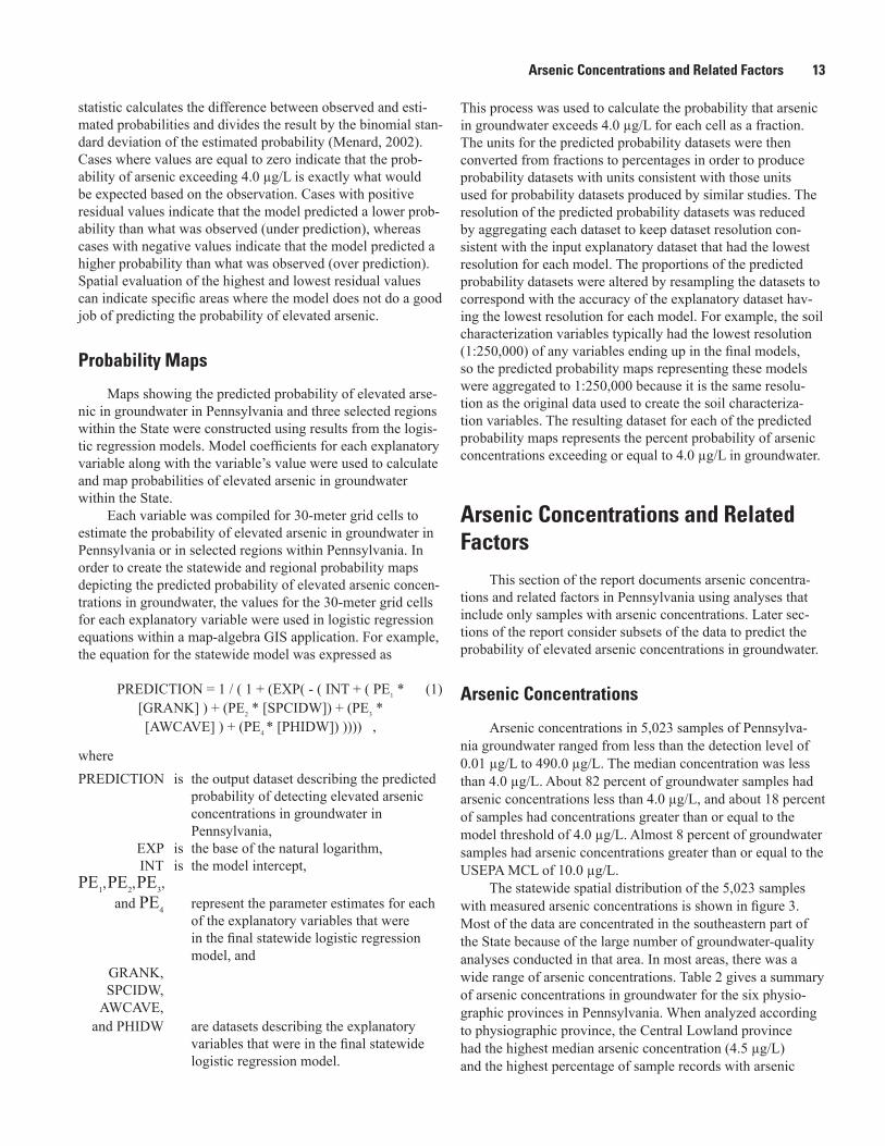
Arsenic Concentrations and Related Factors 13
statistic calculates the difference between observed and esti-mated probabilities and divides the result by the binomial stan-dard deviation of the estimated probability (Menard, 2002). Cases where values are equal to zero indicate that the prob-ability of arsenic exceeding 4.0 µg/L is exactly what would be expected based on the observation. Cases with positive residual values indicate that the model predicted a lower prob-ability than what was observed (under prediction), whereas cases with negative values indicate that the model predicted a higher probability than what was observed (over prediction). Spatial evaluation of the highest and lowest residual values can indicate specific areas where the model does not do a good job of predicting the probability of elevated arsenic.
Probability Maps
Maps showing the predicted probability of elevated arse-nic in groundwater in Pennsylvania and three selected regions within the State were constructed using results from the logis-tic regression models. Model coefficients for each explanatory variable along with the variable’s value were used to calculate and map probabilities of elevated arsenic in groundwater within the State.
Each variable was compiled for 30-meter grid cells to estimate the probability of elevated arsenic in groundwater in Pennsylvania or in selected regions within Pennsylvania. In order to create the statewide and regional probability maps depicting the predicted probability of elevated arsenic concen-trations in groundwater, the values for the 30-meter grid cells for each explanatory variable were used in logistic regression equations within a map-algebra GIS application. For example, the equation for the statewide model was expressed as
PREDICTION = 1 / ( 1 + (EXP( - ( INT + ( PE1 * (1) [GRANK] ) + (PE2 * [SPCIDW]) + (PE3 * [AWCAVE] ) + (PE4 * [PHIDW]) )))) ,
where PREDICTION is the output dataset describing the predicted
probability of detecting elevated arsenic concentrations in groundwater in Pennsylvania,
EXP is the base of the natural logarithm, INT is the model intercept, PE1, PE2, PE3, and PE4 represent the parameter estimates for each
of the explanatory variables that were in the final statewide logistic regression model, and
GRANK, SPCIDW, AWCAVE, and PHIDW are datasets describing the explanatory
variables that were in the final statewide logistic regression model.
This process was used to calculate the probability that arsenic in groundwater exceeds 4.0 µg/L for each cell as a fraction. The units for the predicted probability datasets were then converted from fractions to percentages in order to produce probability datasets with units consistent with those units used for probability datasets produced by similar studies. The resolution of the predicted probability datasets was reduced by aggregating each dataset to keep dataset resolution con-sistent with the input explanatory dataset that had the lowest resolution for each model. The proportions of the predicted probability datasets were altered by resampling the datasets to correspond with the accuracy of the explanatory dataset hav-ing the lowest resolution for each model. For example, the soil characterization variables typically had the lowest resolution (1:250,000) of any variables ending up in the final models, so the predicted probability maps representing these models were aggregated to 1:250,000 because it is the same resolu-tion as the original data used to create the soil characteriza-tion variables. The resulting dataset for each of the predicted probability maps represents the percent probability of arsenic concentrations exceeding or equal to 4.0 µg/L in groundwater.
Arsenic Concentrations and Related Factors
This section of the report documents arsenic concentra-tions and related factors in Pennsylvania using analyses that include only samples with arsenic concentrations. Later sec-tions of the report consider subsets of the data to predict the probability of elevated arsenic concentrations in groundwater.
Arsenic Concentrations
Arsenic concentrations in 5,023 samples of Pennsylva-nia groundwater ranged from less than the detection level of 0.01 µg/L to 490.0 µg/L. The median concentration was less than 4.0 µg/L. About 82 percent of groundwater samples had arsenic concentrations less than 4.0 µg/L, and about 18 percent of samples had concentrations greater than or equal to the model threshold of 4.0 µg/L. Almost 8 percent of groundwater samples had arsenic concentrations greater than or equal to the USEPA MCL of 10.0 µg/L.
The statewide spatial distribution of the 5,023 samples with measured arsenic concentrations is shown in figure 3. Most of the data are concentrated in the southeastern part of the State because of the large number of groundwater-quality analyses conducted in that area. In most areas, there was a wide range of arsenic concentrations. Table 2 gives a summary of arsenic concentrations in groundwater for the six physio-graphic provinces in Pennsylvania. When analyzed according to physiographic province, the Central Lowland province had the highest median arsenic concentration (4.5 µg/L) and the highest percentage of sample records with arsenic

14 Arsenic Concentrations, Environmental Factors, and the Probability of Elevated Arsenic in Groundwater in Pa.
Base
from
U.S
. Bur
eau
of th
e Ce
nsus
dig
ital d
ata,
199
0b 1
:100
,000
Al
bers
Equ
al-A
rea
Coni
c pr
ojec
tion:
Sta
ndar
d Pa
ralle
ls 4
0° N
and
42
° N
, Cen
tral M
erid
ian
-78°
W, L
atitu
de o
f Orig
in 3
9°
Coun
ty b
ound
arie
s fro
m U
.S. B
urea
u of
the
Cens
us, 1
990a
19
90a
Glac
ial a
quife
r sys
tem
bo
unda
ry fr
om P
enns
ylva
nia
Geol
ogic
al S
urve
y, 1
995;
Sol
ler &
Pac
kard
, 199
8Ge
ttysb
urg
and
New
ark
Basi
n bo
unda
ries
from
Pen
nsyl
vani
a Ge
olog
ical
Sur
vey,
200
1
NE
W J
ER
SEY
MA
RY
LA
ND
WE
ST V
IRG
INIA
OH
IO
NE
W Y
OR
K
EXPL
AN
ATI
ON
Ars
enic
con
cent
ratio
ns, i
n m
icro
gram
s pe
r lite
r (n
= 5,
023)
DELAWARE
Grea
ter t
han
or e
qual
to 4
.0 (n
= 9
09)
Less
than
4.0
(n =
4,1
14)
Lake
Eri
e
75°0
0’76
°00’
77°0
0’79
°00’
80°0
0’78
°00’
42°
00’
41°
00’
40°
00’
39°
00’
025
MIL
ES12
.5
025
KIL
OMET
ERS
12.5
Figu
re 3
. Lo
catio
n of
sam
plin
g si
tes
and
asso
ciat
ed re
porte
d ar
seni
c co
ncen
tratio
ns in
gro
undw
ater
in P
enns
ylva
nia,
196
9–20
07. (
N, n
umbe
r of s
ampl
es. A
rsen
ic c
once
n-
tratio
ns a
re s
how
n as
ele
vate
d if
grea
ter t
han
or e
qual
to 4
.0 m
icro
gram
s pe
r lite
r. Da
ta fr
om L
ow a
nd C
hich
este
r (20
06) a
nd L
ow a
nd o
ther
s (2
008)
)

Arsenic Concentrations and Related Factors 15
Table 2. Summary of arsenic concentrations in groundwater (1969–2007) for the six physiographic provinces in Pennsylvania.
[μg/L, micrograms per liter; <, less than]
Physiographic province
Number of sample records
Median arsenic concentration,
in μg/L
Maximum arsenic concentration,
in μg/L
Sample records with arsenic concentrations greater than
or equal to 4.0 μg/L, in percent
Sample records with arsenic concentrations greater than
or equal to 10.0 μg/L, in percent
Appalachian Plateaus 1,870 <4.0 490.0 19 9Atlantic Coastal Plain 52 <4.0 50.0 35 19Central Lowland 76 4.5 293.0 59 43New England 87 <4.0 20.0 14 6Piedmont 1,637 <4.0 85.5 15 5Ridge and Valley 1,301 <4.0 230.0 18 6
concentrations greater than or equal to 4.0 µg/L (59 percent) and greater than or equal to 10.0 µg/L (43 percent) (table 2). No formal statistical test was conducted to evaluate arsenic difference according to physiographic provinces or geologic units in Pennsylvania. Geologic units are listed in appendix 2.
Significance of Groundwater-Quality Properties Related to Arsenic
Spearman’s rho was used to investigate possible correla-tions among arsenic and 31 other groundwater-quality proper-ties and constituents: pH, specific conductance, dissolved oxygen, carbon dioxide, alkalinity, major ions (calcium, magnesium, sodium, potassium, iron, manganese, chloride, sulfate, silica, and fluoride), nutrients [nitrate plus nitrite as nitrogen (N), ammonia, phosphate, total organic carbon], and trace elements (aluminum, barium, cadmium, chromium, cobalt, copper, lead, mercury, nickel, selenium, strontium, and zinc). Some of these constituents, such as dissolved oxygen, iron, manganese, sulfate, nitrate, ammonia, and total organic carbon, could be related to the redox environment as described in the next section. Others may have a common source or have mobility similar to that of arsenic, considering variations in redox and pH. Correlations between arsenic and groundwater-quality constituents were examined on a statewide basis, and those groundwater-quality constituents that were statistically significant (p<0.0001) and had Spearman’s rho values of at least 0.10 in the statewide analysis were also examined on a major aquifer basis to determine how correlations vary in the State according to major aquifer type. Correlations may differ by lithology if examined according to geologic unit because geochemical controls on arsenic occurrence and mobility in groundwater may differ locally across the State according to lithology.
For the statewide dataset, a total of 17 constituents and physical properties had correlations with arsenic that were statistically significant (p<0.0001), with Spearman’s rho values of at least 0.10 (table 3). Out of these 17 constituents and physical properties, 1, 0, 10, and 7 had correlations with
arsenic that were statistically significant (p<0.0001), with Spearman’s rho values of at least 0.10 for the carbonate, crys-talline, siliciclastic, and surficial major aquifers, respectively. In order of decreasing magnitude of Spearman’s rho for the statewide analysis, cobalt, strontium, nickel, sodium, barium, specific conductance, aluminum, alkalinity, manganese, iron, silica, calcium, pH, sulfate, and total organic carbon were positively correlated with arsenic, whereas dissolved oxygen and nitrate plus nitrite (as N) were inversely correlated with arsenic. Positive and inverse correlations for the major aquifer analyses were the same as the statewide analysis.
The statewide correlation of arsenic with cobalt, strontium, nickel, sodium, barium, aluminum, and calcium indicates that these constituents may occur with arsenic in the geologic environment, and in some cases, they may be mobilized under similar chemical conditions. Correlations of arsenic with these constituents also occurred in the siliciclastic major aquifer; correlations of arsenic with sodium and barium occurred in the surficial major aquifer. This finding indicates that these constituents occur with arsenic in the siliciclastic major aquifer geologic environment and may be mobilized under chemical conditions occurring in this major aquifer.
Statewide correlations with specific conductance, pH, alkalinity, and calcium may reflect greater releases of traces of arsenic with increasing dissolution of major minerals or the tendency for arsenic to be mobilized (desorbed) under alkaline conditions. In uncontaminated water, and except for carbonate aquifers, higher specific conductance values often are associated with older water, which has a higher residence time in fractures and other secondary openings than in soils and sediments and greater contact with minerals, leading to increased hardness, alkalinity, and arsenic concentrations in the water. Correlations with specific conductance and calcium occurred for the siliciclastic major aquifer, and correlations with specific conductance and alkalinity occurred for the surfi-cial major aquifer.
Positive correlations of arsenic with iron, total organic carbon and negative correlations of arsenic with dissolved oxygen and nitrate plus nitrite (as N) are consistent with the observation that arsenic may be released by iron oxides
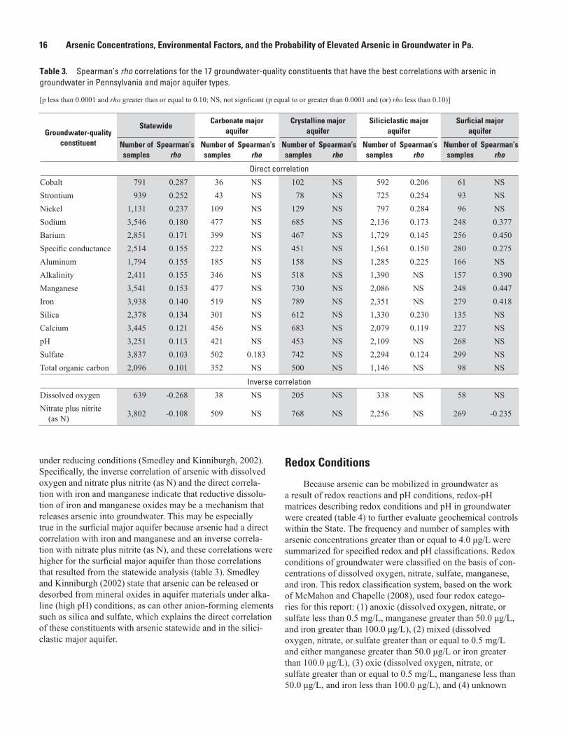
16 Arsenic Concentrations, Environmental Factors, and the Probability of Elevated Arsenic in Groundwater in Pa.
Table 3. Spearman’s rho correlations for the 17 groundwater-quality constituents that have the best correlations with arsenic in groundwater in Pennsylvania and major aquifer types.
[p less than 0.0001 and rho greater than or equal to 0.10; NS, not signficant (p equal to or greater than 0.0001 and (or) rho less than 0.10)]
Groundwater-quality constituent
StatewideCarbonate major
aquiferCrystalline major
aquiferSiliciclastic major
aquiferSurficial major
aquifer
Number of samples
Spearman’s rho
Number of samples
Spearman’s rho
Number of samples
Spearman’s rho
Number of samples
Spearman’s rho
Number of samples
Spearman’s rho
Direct correlation
Cobalt 791 0.287 36 NS 102 NS 592 0.206 61 NSStrontium 939 0.252 43 NS 78 NS 725 0.254 93 NSNickel 1,131 0.237 109 NS 129 NS 797 0.284 96 NSSodium 3,546 0.180 477 NS 685 NS 2,136 0.173 248 0.377Barium 2,851 0.171 399 NS 467 NS 1,729 0.145 256 0.450Specific conductance 2,514 0.155 222 NS 451 NS 1,561 0.150 280 0.275Aluminum 1,794 0.155 185 NS 158 NS 1,285 0.225 166 NSAlkalinity 2,411 0.155 346 NS 518 NS 1,390 NS 157 0.390Manganese 3,541 0.153 477 NS 730 NS 2,086 NS 248 0.447Iron 3,938 0.140 519 NS 789 NS 2,351 NS 279 0.418Silica 2,378 0.134 301 NS 612 NS 1,330 0.230 135 NSCalcium 3,445 0.121 456 NS 683 NS 2,079 0.119 227 NSpH 3,251 0.113 421 NS 453 NS 2,109 NS 268 NSSulfate 3,837 0.103 502 0.183 742 NS 2,294 0.124 299 NSTotal organic carbon 2,096 0.101 352 NS 500 NS 1,146 NS 98 NS
Inverse correlation
Dissolved oxygen 639 -0.268 38 NS 205 NS 338 NS 58 NSNitrate plus nitrite
(as N) 3,802 -0.108 509 NS 768 NS 2,256 NS 269 -0.235
under reducing conditions (Smedley and Kinniburgh, 2002). Specifically, the inverse correlation of arsenic with dissolved oxygen and nitrate plus nitrite (as N) and the direct correla-tion with iron and manganese indicate that reductive dissolu-tion of iron and manganese oxides may be a mechanism that releases arsenic into groundwater. This may be especially true in the surficial major aquifer because arsenic had a direct correlation with iron and manganese and an inverse correla-tion with nitrate plus nitrite (as N), and these correlations were higher for the surficial major aquifer than those correlations that resulted from the statewide analysis (table 3). Smedley and Kinniburgh (2002) state that arsenic can be released or desorbed from mineral oxides in aquifer materials under alka-line (high pH) conditions, as can other anion-forming elements such as silica and sulfate, which explains the direct correlation of these constituents with arsenic statewide and in the silici-clastic major aquifer.
Redox Conditions
Because arsenic can be mobilized in groundwater as a result of redox reactions and pH conditions, redox-pH matrices describing redox conditions and pH in groundwater were created (table 4) to further evaluate geochemical controls within the State. The frequency and number of samples with arsenic concentrations greater than or equal to 4.0 μg/L were summarized for specified redox and pH classifications. Redox conditions of groundwater were classified on the basis of con-centrations of dissolved oxygen, nitrate, sulfate, manganese, and iron. This redox classification system, based on the work of McMahon and Chapelle (2008), used four redox catego-ries for this report: (1) anoxic (dissolved oxygen, nitrate, or sulfate less than 0.5 mg/L, manganese greater than 50.0 μg/L, and iron greater than 100.0 μg/L), (2) mixed (dissolved oxygen, nitrate, or sulfate greater than or equal to 0.5 mg/L and either manganese greater than 50.0 μg/L or iron greater than 100.0 μg/L), (3) oxic (dissolved oxygen, nitrate, or sulfate greater than or equal to 0.5 mg/L, manganese less than 50.0 μg/L, and iron less than 100.0 μg/L), and (4) unknown

Arsenic Concentrations and Related Factors 17
Tabl
e 4.
Re
dox-
pH m
atrix
sho
win
g th
e fre
quen
cy o
f ars
enic
in 5
,023
gro
undw
ater
sam
ples
col
lect
ed s
tate
wid
e in
Pen
nsyl
vani
a, b
y re
dox
clas
sific
atio
n an
d ra
nge
of a
rsen
ic
conc
entra
tions
.
[Val
ues w
ithin
col
ored
blo
cks a
re th
e pe
rcen
tage
and
, in
pare
nthe
ses,
the
num
ber o
f sam
ples
that
exc
eed
the
thre
shol
d of
4 m
icro
gram
s per
lite
r rel
ativ
e to
the
tota
l num
ber o
f sam
ples
for t
he re
dox-
pH
clas
s. R
edox
cla
ssifi
catio
ns a
re b
ased
on
thre
shol
ds o
f McM
ahon
and
Cha
pelle
(200
8) a
nd m
odifi
ed to
four
cla
sses
bec
ause
of d
ata
limita
tions
: (1)
ano
xic
(dis
solv
ed o
xyge
n, n
itrat
e, o
r sul
fate
less
than
0.
5 m
illig
ram
s per
lite
r (m
g/L)
, man
gane
se g
reat
er th
an 5
0.0
mic
rogr
ams p
er li
ter (
μg/L
), an
d iro
n gr
eate
r tha
n 10
0.0
μg/L
), (2
) mix
ed (d
isso
lved
oxy
gen,
nitr
ate,
or s
ulfa
te g
reat
er th
an o
r equ
al to
0.5
mg/
L an
d ei
ther
man
gane
se g
reat
er th
an 5
0.0
μg/L
or i
ron
grea
ter t
han
100.
0 μg
/L),
(3) o
xic
(dis
solv
ed o
xyge
n, n
itrat
e, o
r sul
fate
gre
ater
than
or e
qual
to 0
.5 m
g/L,
man
gane
se le
ss th
an 5
0.0
μg/L
, and
iron
less
th
an 1
00.0
μg/
L), a
nd (4
) unk
now
n (d
ata
for d
isso
lved
oxy
gen,
nitr
ate,
or s
ulfa
te a
nd m
ore
than
one
of t
he o
ther
par
amet
ers w
ere
mis
sing
). %
, per
cent
; n, n
umbe
r]
Redo
x cl
assi
ficat
ion
pH, l
ess
than
4.0
pH, g
reat
er th
an o
r eq
ual t
o 4.
0 an
d le
ss
than
6.0
pH, g
reat
er th
an o
r eq
ual t
o 6.
0 an
d le
ss
than
8.0
pH, g
reat
er th
an o
r eq
ual t
o 8.
0U
nkno
wn
All
sam
ples
in
redo
x cl
assi
fi-ca
tion:
< 1
% (n
= 2
4/50
23)
5 %
(n =
268
/502
3)54
% (n
= 2
729/
5023
)5
% (n
= 2
30/5
023)
35 %
(n =
177
2/50
23)
Ano
xic
8 %
(n =
405
/502
3)75
(n =
3/4
)18
(n =
2/1
1)18
(n =
38/
208)
30 (n
= 1
3/43
)18
(n =
25/
139)
20 (n
= 8
1/40
5)
Mix
ed3
% (n
= 1
29/5
023)
0 (n
= 0
/2)
0 (n
= 0
/11)
15 (n
= 4
/27)
100
(n =
1/1
)8
(n =
7/8
8)9
(n =
12/
129)
Oxi
c30
% (n
= 1
530/
5023
)0
(n =
0/1
)1
(n =
1/8
2)13
(n =
107
/809
)24
(n =
10/
42)
7 (n
= 4
2/59
6)10
(n =
160
/153
0)
Unk
now
n59
% (n
= 2
959/
5023
)59
(n =
10/
17)
14 (n
= 2
3/16
4)16
(n =
269
/168
5)23
(n =
33/
144)
21 (n
= 2
04/9
49)
18 (n
= 5
39/2
959)
All
sam
ples
in p
H c
lass
ifica
tion
54 (n
= 1
3/24
)10
(n =
26/
268)
15 (n
= 4
18/2
729)
25 (n
= 5
7/23
0)16
(n =
278
/177
2)
EXPL
AN
ATI
ON
Perc
enta
ge o
f sam
ples
with
ars
enic
con
cent
ratio
ns
grea
ter t
han
or e
qual
to 4
.0 m
icro
gram
s pe
r lite
r
No
data
0 to
less
than
1
1 to
less
than
10
10 to
less
than
20
20 to
less
than
50
50 o
r mor
e

18 Arsenic Concentrations, Environmental Factors, and the Probability of Elevated Arsenic in Groundwater in Pa.
(data for dissolved oxygen, nitrate, or sulfate and more than one of the other constituents were missing). As a result of the small number of sites with measured dissolved oxygen values (12.7 percent of the dataset), much of the redox classifications (oxic, anoxic, mixed, and unknown) were dependent upon the presence and concentration of nitrate and (or) sulfate and man-ganese and (or) iron. Five general pH classifications were also considered: (1) pH less than 4.0, (2) pH greater than or equal to 4.0 and less than 6.0, (3) pH greater than or equal to 6.0 and less than 8.0, (4) pH greater than or equal to 8.0, and (5) pH concentration unknown.
The frequency of redox conditions of groundwater sam-ples in Pennsylvania was 8 percent of samples were anoxic, 3 percent were mixed, 30 percent were oxic, and 59 percent were unknown (table 4). The frequency of pH classifications of groundwater samples was as follows: 1 percent of samples had pH values less than 4.0, 5 percent had pH values ranging from greater than or equal to 4.0 to less than 6.0, 54 percent had pH values ranging from greater than or equal to 6.0 to less than 8.0, 5 percent had pH values greater than or equal to 8.0, and 35 percent of samples had unknown pH values. In table 4, the percentage of samples within each pH and redox classification with arsenic concentrations greater than or equal to 4.0 μg/L is color coded to highlight those classifications with the greatest frequency of samples with elevated arsenic concentrations.
As groundwater became more reducing, elevated arsenic concentrations were detected more frequently (table 4). For example, 10 percent of oxic waters had elevated arsenic concentrations, as compared to 20 percent of anoxic waters. Also, for a given pH range, more samples with anoxic redox classification more often had elevated arsenic concentrations than samples with oxic or mixed classification. This finding is consistent with the release of arsenic from iron oxides by reductive dissolution of iron oxides or reductive desorption (reduction of arsenate and consequent desorption of arsenite). For oxic and mixed redox classifications, the percentage of samples with elevated arsenic concentrations increased with pH, which is consistent with pH control of arsenate and arse-nite adsorption by iron oxides. Regardless of redox classifica-tion, samples with pH of less than 4.0 or pH of greater than or equal to 8.0 constituted the highest percentages of samples with elevated arsenic concentrations, indicating that both high and low pH may be associated with elevated arsenic. At pH values less than 4.0, iron oxides may not be stable, which is indicated by elevated iron concentrations and low sulfate and iron ratios. Redox/pH matrices show that as waters become more strongly reduced, strongly acidic, or strongly alkaline, arsenic concentrations tend to increase. Elevated pH may provide a geochemical trigger to release arsenic from the iron oxides. Iron and manganese are highly soluble under reducing conditions, which are common in confined aquifers or where groundwater is in contact with organic material. In addition, dissolution of iron oxides may occur in strongly acidic waters.
Predicted Probability of Elevated Arsenic Concentrations in Groundwater
Logistic regression models were created to predict the probability of elevated arsenic concentrations in groundwa-ter in the State of Pennsylvania and to further improve those predictions for three regions within the State: (1) glacial aquifer system, (2) Gettysburg Basin, and (3) Newark Basin (fig. 2). For the purposes of this report, the predictions for the statewide map represent both surficial and bedrock aquifers, which may differ for any given area, because wells known to be completed in bedrock materials and wells known to be completed in glacial and (or) surficial materials were used for the statewide study. The glacial aquifer system consists of the portion of the State encompassed by the extent of the Wiscon-sin glaciation (Pennsylvania Geological Survey, 1995) (fig. 1) and those areas in the northern half of the State overlain by surficial material consisting of coarse-grained sediments (Soller and Packard, 1998) (fig. 1). Only wells known to be completed in glacial materials were used for the glacial aquifer system model, and these wells were also included in the statewide model analysis. The Gettysburg and Newark Basins are located in the Gettysburg-Newark Lowland section of the Piedmont province (fig. 1), with the Gettysburg Basin consist-ing of the southwestern part of the section and the Newark Basin consisting of the northeastern part of the section. The purpose of creating models for these three regions was to cre-ate a model specifically for the glaciated part of the State and to evaluate whether predictions could be improved in these areas of Pennsylvania by including locally specific variables that are not representative of or available across the entire State. These regional models were created using explanatory variables that were available or statistically significant only for certain regions within the State.
Model development included univariate and multivari-ate logistic regression analyses. Univariate relations between elevated arsenic concentrations and explanatory variables were evaluated and are summarized in appendix 3; coefficients indicate the nature of the univariate relation. An alpha level of 0.20 was chosen as the inclusion criterion for selecting explan-atory variables for the multivariate analysis because Hosmer and Lemeshow (1989) indicate that a traditional alpha level of 0.10 failed to identify variables known to be important during some logistic regression analyses. The number of explanatory variables selected for multivariate analyses varied according to study area: 30 out of 40 variables statewide, 32 out of 40 variables for the glacial aquifer system, 23 out of 38 vari-ables for the Gettysburg Basin, and 20 out of 40 variables for the Newark Basin. Coefficients from the final statewide and regional multivariate logistic regression models were used to construct maps illustrating the probability of arsenic concen-trations equaling or exceeding 4.0 µg/L in groundwater in Pennsylvania and in selected regions within the State.

Predicted Probability of Elevated Arsenic Concentrations in Groundwater 19
Statewide
The results of the final statewide model are summarized in table 5 and show the overall fit for the statewide model is statistically significant with a Wald Chi-Square probability value of less than 0.0001. Explanatory variables included in the statewide model are the siliciclastic major aquifer type (SIL), surficial major aquifer type (SURF), estimated ground-water specific conductance (SPCIDW), estimated groundwa-ter pH (PHIDW), and average soil available water capacity (AWCAVE). The standardized regression coefficient (table 5) allows for comparisons among variables in the model in common units where units differed among variables (Menard, 2002). This statistic showed that presence or absence of the siliciclastic and surficial major aquifer types were the most significant variables in the model. SIL, SURF, SPCIDW, and PHIDW showed positive correlations with elevated arsenic concentrations. When the siliciclastic or surficial aquifer types are present, arsenic concentrations increase, which illustrates the potential of primarily siliciclastic and surficial geologic units to affect elevated arsenic concentrations. The positive correlation between elevated arsenic concentrations and the SPCIDW and PHIDW variables describes how groundwater geochemistry can be an indicator of elevated arsenic con-centrations in groundwater. Also, the positive correlation between elevated arsenic concentrations and the SPCIDW and PHIDW variables illustrates how groundwater geochemical properties, such as groundwater specific conductance and pH, can increase the potential for arsenic mobilization, which is consistent with other studies where increased pH was shown to mobilize arsenic (Ayotte and others, 2006). Increases in pH can occur due to ion exchange with sodium, and high specific conductance in groundwater may indicate high amounts of salt (Schlottmann and others, 1998). The only variable with a negative relation with elevated arsenic concentrations was AWCAVE (appendix 3 and table 5), indicating that if a soil has the capability of storing smaller amounts of water, the potential for elevated arsenic concentrations in groundwa-ter increases. This relation suggests that the probability of elevated arsenic concentrations increases beneath sandy and loamy soils, which are more prone to leaching and may show how soils that poorly store water may serve as pathways for arsenic to enter groundwater (U.S. Department of Agriculture, 2008). This is a problem especially if arsenic is present on the land surface from contaminated soils (such as from land appli-cation of pesticides, mining and ore processing operations, or waste disposal) or mineral deposits because arsenic is more prone to leach from these soils into groundwater. Therefore, groundwater vulnerability to elevated arsenic concentrations in Pennsylvania may be characterized as a function of aquifer type and its associated groundwater geochemistry parameters (pH and specific conductance), along with the ability of over-lying soils to store water.
Overall model fit is good with an H-L p-value of 0.2751 (p-values greater than 0.05 indicate good model fit). The gen-eralized r-square value was 0.0709, and the maximum-rescaled
r-square value was 0.1161. Percent concordance was 69.2 percent, and model sensitivity was 22.1. Model discrimi-nation was acceptable, as indicated by a c statistic of 0.695. Diagnostic statistics indicated a lack of multicollinearity for all explanatory variables for the statewide model. Multicollinear-ity diagnostic statistics indicate no detection of multicollinear-ity among model variables. Tolerance values were greater than 0.4 and VIF values were less than 2.5.
Linear regressions between the actual probability of elevated arsenic concentrations and the average predicted probabilities were constructed according to 10 percent deciles calculated with the statewide model calibration data. The results of the regression confirm good model calibration state-wide in Pennsylvania, with an r-square of 0.9647 (fig. 4).
Spatial distribution of predicted probabilities of elevated arsenic concentrations resulting from the statewide model var-ies across the State and is expressed as a percent probability on a map (fig. 5). The map shows the predicted probability of elevated arsenic in groundwater for both surficial and bedrock aquifers, which may differ in some areas of the State but are not differentiated in figure 5. Probabilities of elevated arsenic concentrations of 20 to 50 percent are more widespread in those parts of the State underlain by siliciclastic and surficial aquifers, which also have the highest potential to act as an arsenic source or mobilizer. Areas with less than 20 percent predicted probability of elevated arsenic concentrations, such as the southwestern part of the State, have soils with high percentages of available water capacity, which can also be indicative of other geologic factors because soil development is related to underlying bedrock lithology, except in glaci-ated areas. Within units having siliciclastic or surficial major aquifers, high predicted probabilities (greater than 30 percent) of elevated arsenic concentrations are most prominent in areas with high groundwater specific conductance and pH.
The Pearson residual statistic was calculated for each well to determine which observations were most poorly fit by the model and to spatially show the model’s predictive error. This statistic calculates the difference between observed and estimated probabilities and divides the result by the binomial standard deviation of the estimated probability (Menard, 2002). Resulting Pearson residuals have a mean equal to 0 and a standard deviation equal to 1. For the 5,009 wells, Pearson residual values include 347 values greater than 2.0 and 3 val-ues less than -2.0. Large positive values account for 7 percent of the dataset, whereas large negative values account for less than 1 percent of the dataset. Spatial locations of Pearson residual values associated with outliers indicate areas where the model is not entirely correct and does not fit the dependent data (fig. 5). The northeastern and north-central parts of the State have the fewest poor predictions, whereas the southeast-ern part of the State has a large cluster of poor predictions. Some poor predictions are spread through the northwestern tier and central parts of the State. These poor predictions can be attributed to the uneven spatial distribution of arsenic in rock and associated groundwater and the inability of the variables in the model to completely capture the diversity of

20 Arsenic Concentrations, Environmental Factors, and the Probability of Elevated Arsenic in Groundwater in Pa.Ta
ble
5.
Sum
mar
y of
sta
tistic
s fo
r sta
tew
ide
and
regi
onal
logi
stic
regr
essi
on m
odel
s pr
edic
ting
the
prob
abili
ty o
f ars
enic
exc
eedi
ng 4
.0 m
icro
gram
s pe
r lite
r sta
tew
ide
and
in
thre
e re
gion
s in
Pen
nsyl
vani
a.
[--,
no d
ata;
<, l
ess t
han;
m, m
eter
; %, p
erce
nt; μ
S, m
icro
siem
ens;
cm
, cen
timet
er; g
, gra
ms;
cm
³, cu
bic
cent
imet
er; h
r, ho
ur; H
-L, H
osm
er-L
emes
how
goo
dnes
s-of
-fit t
est;
VIF
, var
ianc
e in
flatio
n fa
ctor
]
Mod
el
Stat
istic
ally
sig
nific
ant e
xpla
nato
ry v
aria
bles
Vari
able
resu
ltsM
odel
fit
Mul
ticol
linea
rity
di
agno
stic
s
Expl
anat
ory
va
riab
leD
escr
iptio
nPa
ram
eter
es
timat
e
Wal
d Ch
i-sq
uare
pr
obab
ility
(p
-val
ue)
Stan
dard
ized
re
gres
sion
co
effic
ient
H-L
(p
-val
ue)
Gen
eral
ized
r-
squa
re
Max
imum
re
scal
ed
r-sq
uare
Perc
ent
conc
orda
ntSe
nsiti
vity
(%
)
c (a
rea
unde
r the
Re
ceiv
er o
pera
ting
char
acte
rist
ic c
urve
)To
lera
nce
VIF
Stat
ewid
e
Inte
rcep
tM
odel
inte
rcep
t-4
.198
7<0
.000
1-
0.27
510.
0709
0.11
6169
.222
.10.
695
--
SIL
Silic
icla
stic
maj
or a
quife
r typ
e (1
= si
licic
last
ic,
0 =
all o
ther
)0.
8697
<0.0
001
0.23
270.
6258
41.
5978
5
SUR
FSu
rfici
al m
ajor
aqu
ifer t
ype
(1 =
surfi
cial
, 0
= al
l oth
er)
1.44
32<0
.000
10.
2289
0.74
451.
3431
9
SPC
IDW
Estim
ated
gro
undw
ater
spec
ific
cond
ucta
nce
(μS/
cm)
0.00
0701
<0.0
001
0.20
710.
9584
11.
0433
9
PHID
WEs
timat
ed g
roun
dwat
er p
H0.
4189
<0.0
001
0.17
220.
9376
71.
0664
8
AWC
AVE
Aver
age
soil
avai
labl
e w
ater
cap
acity
(%)
-11.
3568
<0.0
001
-0.1
417
0.74
158
1.34
847
Gla
cial
aq
uife
r sy
stem
Inte
rcep
tM
odel
inte
rcep
t-1
5.89
490.
0004
-
0.44
770.
2314
0.32
9777
.855
.60.
780
--
BD
AVE
Aver
age
soil
bulk
den
sity
(g/c
m³)
6.54
550.
0165
0.35
760.
9520
91.
0503
2
WET
AVE
Aver
age
wet
land
s lan
d co
ver w
ithin
a 5
00-m
ra
dius
(%)
0.03
920.
0115
0.28
960.
7674
11.
3030
9
SPC
IDW
GLA
CEs
timat
ed g
roun
dwat
er sp
ecifi
c co
nduc
tanc
e us
ing
only
gla
cial
dat
a (μ
S/cm
)0.
0024
20.
0013
0.27
930.
7877
91.
2693
7
PER
MAV
EAv
erag
e so
il pe
rmea
bilit
y (c
m/h
r)0.
1318
0.01
640.
2039
0.82
167
1.21
703
PHID
WG
LAC
Estim
ated
gro
undw
ater
pH
usi
ng o
nly
glac
ial
data
0.53
920.
0288
0.20
170.
8871
71.
1271
8
Get
tysb
urg
Bas
in
Inte
rcep
tM
odel
inte
rcep
t-1
2.46
390.
0056
-
0.92
440.
2428
0.36
5583
.365
.90.
833
--
SAN
DAV
EAv
erag
e so
il sa
nd c
onte
nt (%
)0.
237
0.04
060.
6875
0.94
178
1.06
182
ELEV
Land
surf
ace
elev
atio
n ab
ove
sea
leve
l (m
, Nor
th
Am
eric
an V
ertic
al D
atum
of 1
988)
-0.0
182
0.00
27-0
.452
10.
8627
11.
1591
3
TRI
Dis
tanc
e to
toxi
c ch
emic
al re
leas
e in
vent
ory
site
s (m
)-0
.000
250.
0053
-0.3
705
0.93
638
1.06
794
PHID
WEs
timat
ed g
roun
dwat
er p
H1.
0117
0.00
960.
3542
0.86
822
1.15
178
SPC
IDW
Estim
ated
gro
undw
ater
spec
ific
cond
ucta
nce
(μS/
cm)
0.00
290.
0473
0.24
390.
7558
91.
3229
5
New
ark
B
asin
Inte
rcep
tM
odel
inte
rcep
t-6
.606
90.
0143
-
0.57
380.
1331
0.18
6072
.774
.10.
729
--
PHID
WEs
timat
ed g
roun
dwat
er p
H1.
4425
<0.0
001
0.37
340.
9832
41.
0170
5
SPC
IDW
Estim
ated
gro
undw
ater
spec
ific
cond
ucta
nce
(μs/
cm)
0.00
115
0.02
250.
2809
0.97
962
1.02
080
MU
N
Dis
tanc
e to
mun
icip
aliti
es c
onta
inin
g w
ater
su
pplie
rs w
ith a
rsen
ic tr
eatm
ent a
nd si
tes o
r gr
ound
wat
er in
nee
d of
rem
edia
tion
beca
use
of a
rsen
ic c
onta
min
atio
n (m
)
-0.0
0011
0.01
13-0
.184
60.
8798
31.
1365
9
AWC
AVE
Aver
age
soil
avai
labl
e w
ater
cap
acity
(%)
-42.
294
0.01
41-0
.173
70.
8988
41.
1125
4

Predicted Probability of Elevated Arsenic Concentrations in Groundwater 21
y = 0.9246x + 1.3574R 2 = 0.9647
0
10
20
30
40
50
60
Obse
rved
det
ectio
ns, i
n pe
rcen
t
Statewide n = 5,009
0 10 20 30 40 50 60
y = 0.9497x + 1.4624R 2 = 0.9487
0102030405060708090
100
Average predicted probability, in percent
0 10 20 30 40 50 60 70 80 90 100
Glacial aquifer system n = 307
y = 0.9887x + 0.3272R 2 = 0.9820
0
10
20
30
40
50
60
70
80
Average predicted probability, in percent
0 10 20 30 40 50 60 70 80
Gettysburg Basin n = 174
y = 0.9236x + 2.4701R 2 = 0.9295
0
10
20
30
40
50
60
70
80
0 10 20 30 40 50 60 70 80
Newark Basin n = 455
Figure 4. Percentage of observed detections of elevated arsenic concentrations in relation to the average predicted probability of detecting elevated arsenic concentrations in groundwater statewide and in three regions in Pennsylvania.
the geologic, soil, and geochemical properties controlling arsenic in the State; additional variables or separate models for regions would be needed to seamlessly characterize elevated concentrations of arsenic across the entirety of Pennsylvania.
Glacial Aquifer System
The results of the glacial aquifer system model, which includes the late Wisconsinian glacial border (Pennsylvania Geological Survey, 1995) and areas in the northern half of Pennsylvania that are overlain by surficial material consist-ing of coarse-grained sediments (Soller and Packard, 1998) (fig. 2), are summarized in table 5. The overall fit for the model is statistically significant with a Wald Chi-Square prob-ability value of 0.0004. Explanatory variables included in the glacial aquifer system model are average soil bulk density (BDAVE), average wetlands land cover within a 500-meter radius (WETAVE), specific conductance in groundwater estimated using only glacial data (SPCIDWGLAC), average soil permeability (PERMAVE), and groundwater pH esti-mated using only glacial data (PHIDWGLAC). Results of the standardized regression show that average soil bulk density
is the most significant variable in the model, and all variables showed positive correlations with elevated arsenic concen-trations. High soil bulk density is related to a greater degree of soil compaction and may be an indicator of sandy soils because total pore space in sandy soils commonly is less than total pore space in clay or silt (U.S. Department of Agricul-ture, 2008). Arsenic concentrations increase as average soil permeability increases ( appendix 3 and table 5), which indi-cates that areas of sandy soils with high permeability estimates tend to have higher concentrations of arsenic in groundwater than areas with other soil types. Areas in the glacial aqui-fer system with sandy or coarse-grained deposits are typi-cally associated with glacial valley-fill deposits that overlay fine-grained deposits of till or clay in some places; sediment texture typically is not uniform with depth in glaciated regions (Thomas, 2007). The sandy soils may also exist as a thin veneer that overlies fine-grained till or clay deposits that form the valley walls and (or) terraces. Extensive clay deposits (glacial lake sediments) are found in many glacial valleys and where surface depressions exist the clay deposits encompass wetlands such as peat bogs. Average wetlands land cover within a 500-meter radius (WETAVE) has the second highest
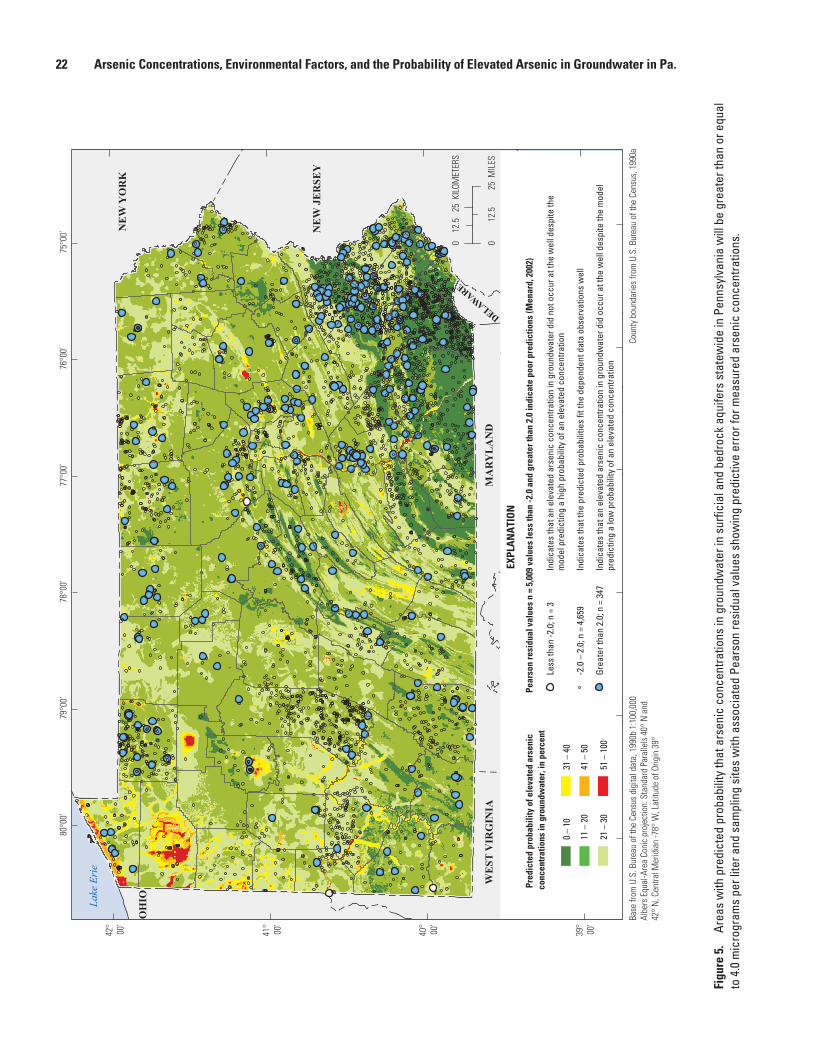
22 Arsenic Concentrations, Environmental Factors, and the Probability of Elevated Arsenic in Groundwater in Pa.
Base
from
U.S
. Bur
eau
of th
e Ce
nsus
dig
ital d
ata,
199
0b 1
:100
,000
Al
bers
Equ
al-A
rea
Coni
c pr
ojec
tion:
Sta
ndar
d Pa
ralle
ls 4
0° N
and
42
° N
, Cen
tral M
erid
ian
-78°
W, L
atitu
de o
f Orig
in 3
9°
Coun
ty b
ound
arie
s fro
m U
.S. B
urea
u of
the
Cens
us, 1
990a
199
0a G
laci
al a
quife
r sys
tem
bo
unda
ry fr
om P
enns
ylva
nia
Geol
ogic
al S
urve
y, 1
995;
Sol
ler &
Pac
kard
, 199
8Ge
ttysb
urg
and
New
ark
Basi
n bo
unda
ries
from
Pen
nsyl
vani
a Ge
olog
ical
Sur
vey,
200
1
NE
W J
ER
SEY
MA
RY
LA
ND
WE
ST V
IRG
INIA
OH
IO
NE
W Y
OR
K
EXPL
AN
ATI
ON
Pred
icte
d pr
obab
ility
of e
leva
ted
arse
nic
conc
entr
atio
ns in
gro
undw
ater
, in
perc
ent
Less
than
-2.0
; n =
3
Grea
ter t
han
2.0;
n =
347
-2.0
– 2
.0; n
= 4
,659
Indi
cate
s th
at th
e pr
edic
ted
prob
abili
ties
fit th
e de
pend
ent d
ata
obse
rvat
ions
wel
l
Indi
cate
s th
at a
n el
evat
ed a
rsen
ic c
once
ntra
tion
in g
roun
dwat
er d
id n
ot o
ccur
at t
he w
ell d
espi
te th
e m
odel
pre
dict
ing
a hi
gh p
roba
bilit
y of
an
elev
ated
con
cent
ratio
n
Indi
cate
s th
at a
n el
evat
ed a
rsen
ic c
once
ntra
tion
in g
roun
dwat
er d
id o
ccur
at t
he w
ell d
espi
te th
e m
odel
pr
edic
ting
a lo
w p
roba
bilit
y of
an
elev
ated
con
cent
ratio
n
Pear
son
resi
dual
val
ues
n =
5,00
9 va
lues
less
than
-2.0
and
gre
ater
than
2.0
indi
cate
poo
r pre
dict
ions
(Men
ard,
200
2)
0 –
10
11 –
20
21 –
30
31 –
40
41 –
50
51 –
100
Lake
Eri
e
DELAWARE
75°0
0’76
°00’
77°0
0’79
°00’
80°0
0’78
°00’
42°
00’
41°
00’
40°
00’
39°
00’
025
MIL
ES12
.5
025
KIL
OMET
ERS
12.5
Figu
re 5
. Ar
eas
with
pre
dict
ed p
roba
bilit
y th
at a
rsen
ic c
once
ntra
tions
in g
roun
dwat
er in
sur
ficia
l and
bed
rock
aqu
ifers
sta
tew
ide
in P
enns
ylva
nia
will
be
grea
ter t
han
or e
qual
to
4.0
mic
rogr
ams
per l
iter a
nd s
ampl
ing
site
s w
ith a
ssoc
iate
d Pe
arso
n re
sidu
al v
alue
s sh
owin
g pr
edic
tive
erro
r for
mea
sure
d ar
seni
c co
ncen
tratio
ns.

Predicted Probability of Elevated Arsenic Concentrations in Groundwater 23
standardized coefficient in the model, which means that the greater the percentage of wetlands within a 500-meter radius, the higher the probability of an elevated arsenic concentration in groundwater. Because many of the glacial valley-fill depos-its identified by the bulk density and permeability of soils are overlain by wetlands, underlying till or clay may be creating a confining layer close to the land surface. This finding suggests that arsenic is being mobilized in these areas in part because of the confining layers that create the wetlands in the glacial valleys. Wetlands, which relate to low dissolved oxygen and redox, could be the result of the upward flow of groundwater. These poorly drained areas can lead to high pH and arsenic desorption. The positive correlation between elevated arsenic concentrations and SPCIDWGLAC and PHIDWGLAC vari-ables describes groundwater geochemistry as an indicator of elevated arsenic concentrations in groundwater in the glacial aquifer system. Increases in pH can cause arsenic to become mobilized in water. Increases in specific conductance indicate older, less oxic water, which can result in the mobilization of arsenic. In inundated areas such as wetlands, groundwater is anoxic and organic rich, and flow is restricted, which allows arsenic to be released. The glacial aquifer system model illustrates that groundwater geochemical properties, such as high groundwater specific conductance and pH, may be acting as geochemical triggers and releasing arsenic from the aquifer matrix to the groundwater in the glacial aquifer system (Thomas, 2007).
Model fit was very good with an H-L p-value of 0.4477. The glacial aquifer system model had a generalized r-square value of 0.2314 with a maximum-rescaled r-square value of 0.3297. According to the percent concordant, 77.8 percent of responses were correctly predicted, and the sensitivity value was 55.6. Model discrimination was acceptable with a c statistic of 0.780. Diagnostic statistics indicated a lack of multicollinearity for all explanatory variables because the lowest Tolerance value was 0.76741 (greater than 0.4), and the highest VIF value was 1.30309 (less than 2.5).
Linear regressions between the actual probability of elevated arsenic concentrations and the average predicted probabilities were constructed according to 10 percent deciles calculated with the glacial aquifer system model calibration data. Regression results confirm good model calibration with an r-square of 0.9487 (fig. 4).
Predicted probabilities of elevated arsenic concentrations produced by the glacial aquifer system model were calculated using arsenic concentration data that were known to repre-sent the glacial units in order to create a model distinguishing between the glacial units and the underlying bedrock. Pre-dicted probabilities for the glacial aquifer system model have a different spatial distribution than probabilities of elevated arsenic resulting from the statewide model that represents underlying bedrock (figs. 5–6). The predicted probabilities of elevated arsenic in groundwater are much greater in the north-western than in the northeastern glacial tier. High predicted probabilities (greater than 50 percent) of elevated arsenic con-centrations are most prominent in areas with high estimated
groundwater specific conductance and pH, which were calcu-lated only for those wells finished in the glacial aquifer sys-tem. These areas are located along Lake Erie in the northwest-ern glacial tier and in areas with glacial valley-fill deposits that correspond to high percentages of wetlands. Probabilities of elevated arsenic concentrations of 20 to 50 percent are more widespread in those areas with high average soil bulk density and high soil permeability; most of these areas are located in the northwestern glacial tier. Areas with the lowest estimated specific conductance and pH, such as the northeastern glacial tier, have less than 20 percent predicted probability of elevated arsenic concentrations.
The Pearson residual statistic was calculated for each well and plotted on a map to determine which observations and spatial areas were most poorly fit by the model and to spa-tially show the model’s predictive error. Results indicate Pear-son residuals have a mean equal to 0 and standard deviation equal to 1. For the 307 wells, Pearson residual values include 16 values greater than 2.0 and two values less than -2.0. Large positive values account for 5 percent of the dataset, whereas large negative values account for less than 1 percent of the dataset. Spatial locations of Pearson residual outliers appear to be randomly distributed throughout the region (fig. 6).
Gettysburg Basin
Results for the Gettysburg Basin model, which represents south-central Pennsylvania, show the overall model fit is sta-tistically significant with a Wald Chi-Square probability value of 0.0056 (table 5). Explanatory variables in the model include average soil sand content (SANDAVE), land-surface elevation above sea level (NAVD 88) (ELEV), distance to toxic chemi-cal release inventory sites (TRI), average estimated groundwa-ter pH (PHIDW), and estimated groundwater specific conduc-tance (SPCIDW). Standardized regression coefficients show that average soil sand content is the most significant variable in the model. SANDAVE, PHIDW, and SPCIDW were posi-tively correlated with elevated arsenic concentrations, whereas ELEV and TRI were negatively correlated. As average soil sand content increases, arsenic concentrations also increase, and as land-surface elevation above NAVD 88 decreases, arsenic concentrations increase. Soils with high sand content seem to be found mostly in the parts of the region with lower land-surface elevations, which seems to correspond to hornfels bordering diabase intrusions with associated mineral deposits of hydrothermal origin, which Senior and Sloto (2006) also found to have locally elevated arsenic concentrations. Sandy soils and low land-surface elevations may be indicators of the underlying geologic environment acting as an arsenic source or mobilizer, causing elevated arsenic concentrations in groundwater within the Gettysburg Basin. The positive cor-relation between elevated arsenic concentrations and SPCIDW and PHIDW variables indicate groundwater geochemistry conditions that facilitate arsenic mobilization in groundwater. Geochemical conditions may be further mobilizing arsenic

24 Arsenic Concentrations, Environmental Factors, and the Probability of Elevated Arsenic in Groundwater in Pa.
Base
from
U.S
. Bur
eau
of th
e Ce
nsus
dig
ital d
ata,
199
0b 1
:100
,000
Al
bers
Equ
al-A
rea
Coni
c pr
ojec
tion:
Sta
ndar
d Pa
ralle
ls 4
0° N
and
42
° N
, Cen
tral M
erid
ian
-78°
W, L
atitu
de o
f Orig
in 3
9°
Coun
ty b
ound
arie
s fro
m U
.S. B
urea
u of
the
Cens
us, 1
990a
Gl
acia
l bou
ndar
y fro
m P
enns
ylva
nia
Geol
ogic
al S
urve
y,
1995
and
Sol
ler &
Pac
kard
, 199
8
NE
W J
ER
SEY
MA
RY
LA
ND
WE
ST V
IRG
INIA
OH
IO
NE
W Y
OR
K
EXPL
AN
ATI
ON
Pred
icte
d pr
obab
ility
of e
leva
ted
arse
nic
conc
entr
atio
ns in
gro
undw
ater
, in
perc
ent
Less
than
-2.0
; n =
2
Grea
ter t
han
2.0;
n =
16
-2.0
– 2
.0; n
= 2
89In
dica
tes
that
the
pred
icte
d pr
obab
ilitie
s fit
the
depe
nden
t dat
a ob
serv
atio
ns w
ell
Indi
cate
s th
at a
n el
evat
ed a
rsen
ic c
once
ntra
tion
in g
roun
dwat
er d
id n
ot o
ccur
at t
he w
ell d
espi
te th
e m
odel
pre
dict
ing
a hi
gh p
roba
bilit
y of
an
elev
ated
con
cent
ratio
n
Indi
cate
s th
at a
n el
evat
ed a
rsen
ic c
once
ntra
tion
in g
roun
dwat
er d
id o
ccur
at t
he w
ell d
espi
te th
e m
odel
pr
edic
ting
a lo
w p
roba
bilit
y of
an
elev
ated
con
cent
ratio
n
Pear
son
resi
dual
val
ues
n =
307
valu
es le
ss th
an -2
.0 a
nd g
reat
er th
an 2
.0 in
dica
te p
oor p
redi
ctio
ns (M
enar
d, 2
002)
0 –
10
11 –
20
21 –
30
31 –
40
41 –
50
51 –
100
Lake
Eri
e
DELAWARE
75°0
0’76
°00’
77°0
0’79
°00’
80°0
0’78
°00’
42°
00’
41°
00’
40°
00’
39°
00’
025
MIL
ES12
.5
025
KIL
OMET
ERS
12.5
Figu
re 6
. Ar
eas
with
pre
dict
ed p
roba
bilit
y th
at a
rsen
ic c
once
ntra
tions
in g
roun
dwat
er in
the
glac
ial a
quife
r sys
tem
in P
enns
ylva
nia
will
be
grea
ter t
han
or e
qual
to
4.0
mic
rogr
ams
per l
iter a
nd s
ampl
ing
site
s w
ith a
ssoc
iate
d Pe
arso
n re
sidu
al v
alue
s sh
owin
g pr
edic
tive
erro
r for
mea
sure
d ar
seni
c co
ncen
tratio
ns in
wel
ls.
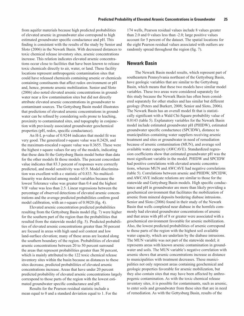
Predicted Probability of Elevated Arsenic Concentrations in Groundwater 25
from aquifer materials because high predicted probabilities of elevated arsenic in groundwater also correspond to high estimated groundwater specific conductance and pH. This finding is consistent with the results of the study by Senior and Sloto (2006) in the Newark Basin. With decreased distances to toxic chemical release inventory sites, arsenic concentrations increase. This relation indicates elevated arsenic concentra-tions occur close to facilities that have been known to release toxic chemicals directly to air, water, or land. These facility locations represent anthropogenic contamination sites that could have released chemicals containing arsenic or chemicals containing constituents that affect redox environment or pH and, hence, promote arsenic mobilization. Senior and Sloto (2006) also noted elevated arsenic concentrations in ground-water near a few contamination sites but did not directly attribute elevated arsenic concentrations in groundwater to contaminant sources. The Gettysburg Basin model illustrates that predictions of elevated arsenic concentrations in ground-water can be refined by considering soils prone to leaching, proximity to contaminated sites, and topography in conjunc-tion with previously associated groundwater geochemical properties (pH, redox, specific conductance).
An H-L p-value of 0.9244 indicates that model fit was very good. The generalized r-square value was 0.2428, and the maximum-rescaled r-square value was 0.3655. These were the highest r-square values for any of the models, indicating that these data fit the Gettysburg Basin model better than data for the other models fit those models. The percent concordant value indicates that 83.3 percent of responses were correctly predicted, and model sensitivity was 65.9. Model discrimina-tion was excellent with a c statistic of 0.833. No multicol-linearity was detected among model variables because the lowest Tolerance value was greater than 0.4 and the highest VIF value was less than 2.5. Linear regressions between the percentage of observed detections of elevated arsenic concen-trations and the average predicted probabilities confirm good model calibration, with an r-square of 0.9820 (fig. 4).
Elevated arsenic concentration predicted probabilities resulting from the Gettysburg Basin model (fig. 7) were higher for the southern part of the region than the probabilities that resulted from the statewide model (fig. 5). Predicted probabili-ties of elevated arsenic concentrations greater than 50 percent are focused in areas with high sand soil content and low land-surface elevation; many of these areas are located along the southern boundary of the region. Probabilities of elevated arsenic concentrations between 20 to 50 percent surround the areas that represent probabilities greater than 50 percent, which is mainly attributed to the 122 toxic chemical release inventory sites within the basin because as distances to these sites decrease, predicted probabilities of elevated arsenic concentrations increase. Areas that have under 20 percent predicted probability of elevated arsenic concentrations largely correspond to those parts of the region with the lowest esti-mated groundwater specific conductance and pH.
Results for the Pearson residual statistic include a mean equal to 0 and a standard deviation equal to 1. For the
174 wells, Pearson residual values include 8 values greater than 2.0 and 0 values less than -2.0; large positive values account for 5 percent of the dataset. The spatial locations for the eight Pearson residual values associated with outliers are randomly spread throughout the region (fig. 7).
Newark Basin
The Newark Basin model results, which represent part of southeastern Pennsylvania northeast of the Gettysburg Basin, have geologic variables that are similar to the Gettysburg Basin, which means that these two models have similar model variables. These two areas were considered separately for this study because the Newark Basin has often been consid-ered separately for other studies and has similar but different geology (Peters and Burkert, 2008; Senior and Sloto, 2006). The Newark Basin has an overall model fit that is statisti-cally significant with a Wald Chi-Square probability value of 0.0143 (table 5). Explanatory variables for the Newark Basin model include estimated groundwater pH (PHIDW), estimated groundwater specific conductance (SPCIDW), distance to municipalities containing water suppliers receiving arsenic treatment and sites or groundwater in need of remediation because of arsenic contamination (MUN), and average soil available water capacity (AWCAVE). Standardized regres-sion coefficients show that estimated groundwater pH was the most significant variable in the model. PHIDW and SPCIDW had positive correlations with elevated arsenic concentra-tions, whereas MUN and AWCAVE had negative correlations (table 5). Correlations between arsenic and PHIDW, SPCIDW, and AWCAVE indicate relations are similar to those for the statewide and Gettysburg Basin models. High specific conduc-tance and pH in groundwater are more than likely providing a geochemical environment that facilitates the mobilization of arsenic from mineral deposits bordering diabase intrusions. Senior and Sloto (2006) found in their study of the Newark Basin that wells completed near diabase in the hornfels com-monly had elevated groundwater concentrations of arsenic and that areas with pH of 8 or greater were associated with a geochemical environment favorable for arsenic mobilization. Also, the lowest predicted probabilities of arsenic correspond to those parts of the region with the highest soil available water capacity, which are underlain by the diabase intrusions. The MUN variable was not part of the statewide model; it represents areas with known arsenic contamination in ground-water and soils. The MUN variable’s negative correlation with arsenic shows that arsenic concentrations increase as distance to municipalities with treatment decreases. These munici-palities not only represent areas containing geochemical and geologic properties favorable for arsenic mobilization, but they also contain sites that may have been affected by anthro-pogenic contamination. As with the toxic chemical release inventory sites, it is possible for contaminants, such as arsenic, to enter soils and groundwater from these sites that are in need of remediation. As with the Gettysburg Basin, results of the
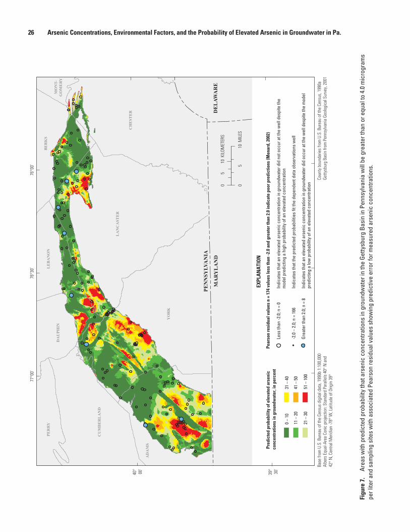
26 Arsenic Concentrations, Environmental Factors, and the Probability of Elevated Arsenic in Groundwater in Pa.
Base
from
U.S
. Bur
eau
of th
e Ce
nsus
dig
ital d
ata,
199
0b 1
:100
,000
Al
bers
Equ
al-A
rea
Coni
c pr
ojec
tion:
Sta
ndar
d Pa
ralle
ls 4
0° N
and
42
° N
, Cen
tral M
erid
ian
-78°
W, L
atitu
de o
f Orig
in 3
9°
Coun
ty b
ound
arie
s fro
m U
.S. B
urea
u of
the
Cens
us, 1
990a
Getty
sbur
g Ba
sin
from
Pen
nsyl
vani
a Ge
olog
ical
Sur
vey,
200
1
EXPL
AN
ATI
ON
Pred
icte
d pr
obab
ility
of e
leva
ted
arse
nic
conc
entr
atio
ns in
gro
undw
ater
, in
perc
ent
Less
than
-2.0
; n =
0
Grea
ter t
han
2.0;
n =
8
-2.0
– 2
.0; n
= 1
66In
dica
tes
that
the
pred
icte
d pr
obab
ilitie
s fit
the
depe
nden
t dat
a ob
serv
atio
ns w
ell
Indi
cate
s th
at a
n el
evat
ed a
rsen
ic c
once
ntra
tion
in g
roun
dwat
er d
id n
ot o
ccur
at t
he w
ell d
espi
te th
e m
odel
pre
dict
ing
a hi
gh p
roba
bilit
y of
an
elev
ated
con
cent
ratio
n
Indi
cate
s th
at a
n el
evat
ed a
rsen
ic c
once
ntra
tion
in g
roun
dwat
er d
id o
ccur
at t
he w
ell d
espi
te th
e m
odel
pr
edic
ting
a lo
w p
roba
bilit
y of
an
elev
ated
con
cent
ratio
n
Pear
son
resi
dual
val
ues
n =
174
valu
es le
ss th
an -2
.0 a
nd g
reat
er th
an 2
.0 in
dica
te p
oor p
redi
ctio
ns (M
enar
d, 2
002)
0 –
10
11 –
20
21 –
30
31 –
40
41 –
50
51 –
100
010
MIL
ES5
010
KIL
OMET
ERS
5
AD
AM
S
CH
EST
ER
MO
NT-
GO
ME
RY
LA
NC
AST
ER
YO
RK
BE
RK
SPE
RR
YL
EB
AN
ON
CU
MB
ER
LA
ND
DA
UPH
IN
PEN
NSY
LVA
NIA
DE
LAW
AR
EM
AR
YL
AN
D
76°0
0’77
°00’
40°
00’
39°
30’
76°3
0’
Figu
re 7
. Ar
eas
with
pre
dict
ed p
roba
bilit
y th
at a
rsen
ic c
once
ntra
tions
in g
roun
dwat
er in
the
Getty
sbur
g Ba
sin
in P
enns
ylva
nia
will
be
grea
ter t
han
or e
qual
to 4
.0 m
icro
gram
s pe
r lite
r and
sam
plin
g si
tes
with
ass
ocia
ted
Pear
son
resi
dual
val
ues
show
ing
pred
ictiv
e er
ror f
or m
easu
red
arse
nic
conc
entra
tions
.

Limitations and Uses of Arsenic Models and Probability Maps 27
Newark Basin model illustrate that geochemical properties of groundwater, soils properties, and proximity to areas contain-ing water suppliers with arsenic treatment or sites in need of remediation because of arsenic contamination describe an environment favorable for arsenic mobilization.
Overall model fit was very good, indicated by an H-L p-value of 0.5738. The generalized r-square value was 0.1331, and the maximum-rescaled r-square value was 0.1860. The percent concordant value indicates that 72.7 percent of responses were correctly predicted, and model sensitivity was 74.1. A c statistic of 0.729 shows acceptable model discrimi-nation. Diagnostic statistics indicate a lack of multicollinear-ity for all explanatory variables for the Newark Basin model. Because the lowest Tolerance value was 0.87983 (all values are greater than 0.4) and the highest VIF value was 1.13659 (all values were less than 2.5), these multicollinearity diagnos-tic statistics indicate that there is no multicollinearity among model variables. Linear regressions between the percentage of observed detections of elevated arsenic concentrations and the average predicted probabilities confirm good model calibra-tion, with an r-square of 0.9295 (fig. 4).
Predicted probabilities of elevated arsenic concentrations resulting from the Newark Basin model (fig. 8) are higher than those probabilities that resulted from the statewide model (fig. 5). Predicted probabilities of elevated arsenic concentra-tions greater than 30 percent are distributed mainly in the central and northern parts of the region and correspond to high estimated groundwater specific conductance and pH and to proximity to municipalities containing water suppliers with arsenic treatment and sites or groundwater in need of remedia-tion because of arsenic contamination. Predicted probabilities less than 30 percent primarily correspond to high percentages of soil available water capacity. These areas are located in the southeastern part of the Newark Basin and in the northern part of the basin where they correspond to diabase intrusions.
Pearson residual results show a mean equal to 0 and stan-dard deviation equal to 1. For the 455 wells, Pearson residual values include 0 values less than -2.0 and 14 values greater than 2.0; large positive values account for 3 percent of the dataset. Spatial locations of Pearson residual values associated with outliers indicate that most poor predictions are located in the southeastern part of the region (fig. 8).
Limitations and Uses of Arsenic Models and Probability Maps
Probability maps developed for this study show the predicted probability of arsenic concentrations greater than or equal to 4.0 µg/L in groundwater in Pennsylvania and three regions within the State, including the glacial aquifer system, the Gettysburg Basin, and the Newark Basin (figs. 5–8). The probability maps do not show actual arsenic contamination of groundwater but rather depict areas that have the potential or likelihood of having groundwater with elevated arsenic
concentrations. There is inherent uncertainty associated with each of the maps, which stems from data quality and availabil-ity in the well database and GIS-based explanatory variables and the estimation errors in the logistic regression coefficients.
Certain areas of the predictive maps may have elevated arsenic that are not characterized by the statewide or regional models and are indicated by areas with many Pearson residu-als indicating poor predictions (values less than -2.0 and greater than 2.0). These areas have greater uncertainty associ-ated with their relative predicted probabilities. The occurrence of Pearson residuals representing poor predictions resulting from the statewide and regional models supports the con-cept that regional models across the entire State or regional models encompassing smaller regions than those analyzed in this study may be needed to improve predicted probabilities. Higher resolution spatial data and additional data on arsenic concentrations in groundwater and associated variables would improve the predictive power of the models. Further study and additional independent data are also needed to validate the results of each logistic regression model.
In addition, regional differences in numerous factors, such as lithology and geochemical controls, affecting arsenic mobility are not accounted for in the statewide model and may reduce the predictive power of the statewide model. For example, the major aquifer type variable present in the statewide analysis is a broad characterization of dominant lithologies and may mask localized mineralogical differences in geologic units within the major aquifers. An example of a geochemical control not accounted for can be seen in table 4 where it shows how elevated concentrations of arsenic tend to occur at low pH (less than 4.0) and high pH (greater than or equal to 8.0), but the statewide Spearman’s rho correlation indicates a positive correlation between arsenic concentra-tions and pH values. This positive correlation between arsenic concentrations and pH values masks the relation of elevated arsenic concentrations to low pH, which may occur in fewer places statewide but still results in arsenic concentrations of concern. Differences in variables that were significant among statewide and regional models also illustrate factors that are not able to be accounted for in the statewide model. It is likely that the regional models for geologic units and major aquifers in other physiographic provinces, such as the Appalachian Plateaus, Atlantic Coastal Plain, Piedmont Uplands, or Ridge and Valley, that were not separately analyzed for this study, would also differ and provide better predictive ability in those regions than the statewide model.
By providing an improved understanding of spatial controls on arsenic statewide and in three regions in Pennsyl-vania, the probability maps developed for this report may help resource managers to prioritize areas for groundwater-quality monitoring or implement alternative management practices. However, the probability maps associated with this report are intended for regional-scale use and have limitations for use at the field-scale or when considering individual wells. The maps are not appropriate at any scale larger than 1:250,000, which is the smallest scale of any of the explanatory variables

28 Arsenic Concentrations, Environmental Factors, and the Probability of Elevated Arsenic in Groundwater in Pa.
LA
NC
AST
ER
DE
LAW
AR
E
PHIL
AD
ELPH
IA
MO
NT
GO
ME
RY
BU
CK
S
SCH
UY
KIL
LN
OR
TH
AM
PTO
N
BE
RK
S
LE
HIG
H
PEN
NSY
LVA
NIA
NE
W J
ER
SEY
CH
EST
ER
05
MIL
ES
05
KIL
OMET
ERS
Base
from
U.S
. Bur
eau
of th
e Ce
nsus
dig
ital d
ata,
199
0b 1
:100
,000
Al
bers
Equ
al-A
rea
Coni
c pr
ojec
tion:
Sta
ndar
d Pa
ralle
ls 4
0° N
and
42
° N
, Cen
tral M
erid
ian
-78°
W, L
atitu
de o
f Orig
in 3
9°
Coun
ty b
ound
arie
s fro
m U
.S. B
urea
u of
the
Cens
us, 1
990a
New
ark
Basi
n fro
m P
enns
ylva
nia
Geol
ogic
al S
urve
y, 2
001
EXPL
AN
ATI
ON
Pred
icte
d pr
obab
ility
of e
leva
ted
arse
nic
conc
entr
atio
ns in
gro
undw
ater
, in
perc
ent
Less
than
-2.0
; n =
0
Grea
ter t
han
2.0;
n =
14
-2.0
– 2
.0; n
= 4
41In
dica
tes
that
the
pred
icte
d pr
obab
ilitie
s fit
the
depe
nden
t dat
a ob
serv
atio
ns w
ell
Indi
cate
s th
at a
n el
evat
ed a
rsen
ic c
once
ntra
tion
in g
roun
dwat
er d
id n
ot o
ccur
at t
he w
ell d
espi
te th
e m
odel
pre
dict
ing
a hi
gh p
roba
bilit
y of
an
elev
ated
con
cent
ratio
n
Indi
cate
s th
at a
n el
evat
ed a
rsen
ic c
once
ntra
tion
in g
roun
dwat
er d
id o
ccur
at t
he w
ell d
espi
te th
e m
odel
pr
edic
ting
a lo
w p
roba
bilit
y of
an
elev
ated
con
cent
ratio
n
Pear
son
resi
dual
val
ues
n =
455
valu
es le
ss th
an -2
.0 a
nd g
reat
er th
an 2
.0 in
dica
te p
oor p
redi
ctio
ns (M
enar
d, 2
002)
0 –
10
11 –
20
21 –
30
31 –
40
41 –
50
51 –
100
75°0
0’76
°00’
40°
00’
40°
30’
75°3
0’
Figu
re 8
. Ar
eas
with
pre
dict
ed p
roba
bilit
y th
at a
rsen
ic c
once
ntra
tions
in g
roun
dwat
er in
the
New
ark
Basi
n in
Pen
nsyl
vani
a w
ill b
e gr
eate
r tha
n or
equ
al to
4.0
mic
rogr
ams
per
liter
and
sam
plin
g si
tes
with
ass
ocia
ted
Pear
son
resi
dual
val
ues
show
ing
pred
ictiv
e er
ror f
or m
easu
red
arse
nic
conc
entra
tions
in w
ells
.

Summary and Conclusions 29
used in the models. The threshold accuracy value for a scale of 1:250,000, as established by National Map Accuracy Stan-dards, is 127 meters (417 feet) in ground units. Concentrations of arsenic in groundwater and in a well are affected by many field-scale complexities that are not accounted for in the mod-els. For example, the models do not account for preferential groundwater flow paths in bedrock units. As a result, although a well may be located in a region with a high predicted prob-ability of elevated arsenic, the well may yield water with low arsenic concentrations as a result of complexities that cannot be represented in the regional-scale models that were developed for this study. Therefore, the models and maps are not appropriate for predicting the risk of elevated arsenic in individual wells.
In addition to the explanatory variables included in each of the four models, there may be other explanatory variables that can affect concentrations of arsenic in groundwater. For example, the regional models do not take geology into account, which means that these regions need to be studied in greater detail. Also, exclusion of an explanatory variable from the model does not mean that the variable does not affect concentrations of arsenic. For example, data on dissolved oxygen concentrations could have been used to define the redox environment, but sufficient data were not available to create a dissolved oxygen dataset for use in the analysis. In addition, for two or more explanatory variables that exhibit strong correlations with one another, all of these variables were not included in the same model because including one variable usually accounts for the effects of the other correlated variables. For example, soil available water capacity and soil thickness have a strong positive correlation, so only one of the variables was included. Additionally, characterization of lithologies other than by the selected major aquifer types may result in different correlations between elevated arsenic con-centrations in groundwater and geologic units. Some geologic units from each major aquifer type may be more likely than other geologic units to have elevated arsenic concentrations, and so the more subtle differences in mineralogy of these units that affects arsenic occurrence and mobility are not captured in the models.
Summary and ConclusionsData on arsenic concentrations in groundwater were
available for 5,023 wells—monitoring, domestic, public supply, commercial, irrigation, and industrial wells—across Pennsylvania. Arsenic was detected at a concentration of 4.0 micrograms per liter (µg/L) or greater in 18 percent of samples. Arsenic concentrations that met or exceeded the U.S. Environmental Protection Agency maximum contami-nant level of 10.0 µg/L were measured in about 8 percent of samples; the highest arsenic concentration was 490.0 µg/L.
Comparison of arsenic concentrations in groundwater by physiographic province indicates that the Central Lowland
province in northwestern Pennsylvania has the highest median arsenic concentration (4.5 µg/L) and highest percentage of sample records with arsenic concentrations greater than or equal to 4.0 µg/L (59 percent) and greater than or equal to 10.0 µg/L (43 percent). Evaluation of arsenic concentrations in groundwater of four major aquifer types in Pennsylvania (carbonate, crystalline, siliciclastic, and surficial) showed that all aquifer types have median arsenic concentrations less than 4.0 µg/L, and the highest arsenic concentration (490.0 µg/L) was in a siliciclastic aquifer. The siliciclastic and surficial aquifers have the highest percentage of sample records with arsenic concentrations greater than or equal to 4.0 µg/L and 10.0 µg/L. Elevated arsenic concentrations, which are those arsenic concentrations greater than or equal to 4.0 µg/L, were most commonly found in strongly reducing groundwater state-wide. Arsenic concentrations were elevated in 10 percent of oxic waters, whereas 20 percent of anoxic waters had elevated arsenic concentrations. Also, for a given pH range, samples classified as anoxic reductive-oxidative (redox) water more typically had elevated arsenic concentrations than samples classified as oxic or mixed. The relatively large percentage of anoxic and high pH waters with elevated concentrations of arsenic indicates that mechanisms such as reductive desorp-tion or dissolution are occurring, releasing arsenic from iron oxides. However, elevated arsenic concentrations were also found in reducing waters with low pH, indicating that other mechanisms, such as reductive dissolution of iron oxides, also may result in mobilization of arsenic in groundwater.
Arsenic concentrations were correlated with concentra-tions of several chemical constituents, including (1) con-stituents linked to redox processes (specific conductance, alkalinity, iron, pH, total organic carbon, dissolved oxygen, and nitrate plus nitrite (as N)), (2) constituents that may be mobilized under chemical conditions similar to those that mobilize arsenic (cobalt, strontium, nickel, sodium, barium, aluminum, and calcium), and (3) anions or oxyanions that sorb to iron oxides (silica and sulfate).
Logistic regression was used to develop spatial statisti-cal models predicting the probability of detecting arsenic concentrations greater than or equal to 4.0 µg/L in ground-water statewide and in three intrastate regions. Although, the statewide and regional (glacial aquifer system, Gettysburg Basin, and Newark Basin) models consisted of slightly differ-ent variables, the results have common characteristics that can be grouped as (1) geologic and soils variables that describe arsenic sources and mobilizers (major aquifer types, soil available water capacity, soil bulk density, soil permeability, and soil sand content), (2) geochemical variables that describe the geochemical environment of the groundwater (specific conductance and pH), and (3) locally specific variables that are unique to each of the three regions studied and are not appli-cable to the statewide analysis (wetlands land cover, land-sur-face elevations above the North American Vertical Datum of 1988 (NAVD 88), distance to toxic chemical release inventory sites, and distance to municipalities containing water suppli-ers with arsenic treatment and sites or groundwater in need of

30 Arsenic Concentrations, Environmental Factors, and the Probability of Elevated Arsenic in Groundwater in Pa.
remediation because of arsenic contamination). These models have limitations because they may not characterize areas that have different controls on arsenic mobility and should not be used to estimate probabilities of elevated arsenic in groundwa-ter at the field-scale or when considering individual wells.
The occurrence of arsenic in groundwater of Pennsyl-vania is largely the result of mobilization of arsenic from natural sources in the aquifer and the geochemical conditions of groundwater. For this investigation, the potential for natural geologic features to be sources of arsenic was established on the basis of selected geologic characteristics (primary lithol-ogy to determine major aquifer type). Also, the data reviewed for this investigation indicate that variations in arsenic concen-trations in Pennsylvania groundwater generally are related to variations in redox conditions, pH, and specific conductance at State and regional scales. As demonstrated in this report, these groundwater-quality variables, which affect the release, transport, and attenuation of arsenic in the aquifer, may be considered in conjunction with siliciclastic and surficial major aquifer types to indicate geologic conditions where ground-water may contain elevated arsenic. Health officials may consider testing or advising homeowners in geologic settings within siliciclastic or surficial major aquifer types to test their groundwater for arsenic, particularly if other available data, such as proximity to known areas of elevated arsenic or arse-nic contaminant release sites or geochemical conditions (low redox, high pH, high specific conductance) indicate a geo-chemical environment that favors the mobilization of arsenic.
References Cited
Allison, P.D., 2001, Logistic regression using the SAS system: Theory and application: Cary, North Carolina, SAS Institute Inc., 288 p.
Ayotte, J.D., Nielsen, M.G., and Robinson, B.R., Jr., 1998, Relation of arsenic concentrations in ground water to bed-rock lithology in eastern New England: Geological Society of America Annual Meeting, Toronto, Ontario, p. A-58.
Ayotte, J.D., Nolan, B.T., Nuckols, J.R., Cantor, K.P., Rob-inson, G.R. Jr, Baris, Dalsu, Hayes, Laura, Karagas, M.R., Bress, William, Silverman, D.T., and Lubin, J.H., 2006, Modeling the probability of arsenic in groundwater in New England as a tool for exposure assessment: Environmental Science & Technology, v. 40, no.11, p. 3578–3585.
Bankey, V., Cuevas, A., Daniels, D., Finn, C.A., Hernandez, I., Hill, P., Kucks, R., Miles, W., Pilkington, M., Roberts, C., Roest, W., Rystrom, V., Shearer, S., Snyder, S., Sweeney, R., Velez, J., Philips, J.D., Ravat, D., 2002, Digital data grids for the magnetic anomaly map of North America: U.S. Geological Survey Open-File Report 02–414, raster digital data.
Benbrahim-Tallaa, Lamia, and Waalkes, M.P., 2007, Inorganic arsenic and human prostate cancer: Environmental Health Perspectives, accessed May 4, 2009, at http://dx.doi.org/doi:10.1289/ehp.10423
Berg, T.M., Barnes, J.H., Sevon, W.D., Skema, V.W., Wilshu-sen, J.P., and Yannacci, D.W., 1989, Physiographic prov-inces of Pennsylvania: Pennsylvania Geological Survey, 4th ser., Map 13 (color), scale 1:2,000,000, 8.5 x 11.
Berg, T.M., Edmunds, W.E., Geyer, A.R., Glover, A.D., Hoskins, D.M., MacLachlan, D.B., Root, S.I., Sevon, W.D., and Socolow, A.A., comps., 1980, Geologic map of Penn-sylvania: Pennsylvania Geological Survey, 4th ser., Map 1, scale 1:250,000, 3 sheets.
Buckwalter, T.F., and Moore, M.E., 2007, Ground-water resources and the hydrologic effects of petroleum occur-rence and development, Warren County, Northwestern Pennsylvania: U.S. Geological Survey Scientific Investiga-tions Report 2006–5263, 86 p.
Chen, Yu, Santella, R.M., Kibriya, M.G., Wang, Qiao, Kapil, Maya, Verret, W.J., Graziano, J.H., and Ahsan, Habibul, 2007, Association between arsenic exposure from drinking water and plasma levels of soluble cell adhesion molecules: Environmental Health Perspectives, accessed May 4, 2009, at http://dx.doi.org/doi:10.1289/ehp.10277.
Cox, D.R., and Snell, E.J., 1989, Analysis of binary data (3rd ed.): Boca Raton, Fla., CRC Press, 236 p.
Cravotta, C.A., III, 2008, Dissolved metals and associated constituents in abandoned coal-mine discharges, Pennsylva-nia, USA – 1. Constituent concentrations and correlations: Applied Geochemistry, v. 23, p. 166–202.
Cuff, D.J., Young, W.J., Muller, E.K., Zelinsky, W., and Abler, R.F., 1989, The Atlas of Pennsylvania: Philadelphia, Pa., Temple University Press, 288 p.
Davey, J.C., Nomikos, A.P., Wungjiranirum, Manida, Sher-man, J.R., Ingram, Liam, Batki, Cavus, Lariviere, J.P., and Hamilton, J.W., 2007, Arsenic as an endocrine disruptor—receptor-mediated gene regulation and thyroid hormone-mediated amphibian tail metamorphosis: Environmental Health Perspectives, accessed May 4, 2009, at http://dx.doi.org/doi:10.1289/ehp.10131.
Eary, L.E., and Schramke, J.A., 1990, Rates of inorganic oxi-dation reactions involving dissolved oxygen, in Melchior, D.C., and Bassett, R.L., eds., Chemical modeling of aque-ous systems II: American Chemical Society Symposium 416, p. 379–396.
Fenneman, N.M., and Johnson, D.W., 1946, Physical divi-sions of the United States: U.S. Geological Survey, scale 1:7,000,000, 1 sheet.

References Cited 31
Foster, A.L., Brown Jr. G.E., Parks, G.A., 2003, XAFS study of As(V) and Se(IV) sorption complexes on hydrous Mn oxides: Geochimica et Cosmochimica Acta, v. 67, no. 11, p. 1937–1953.
Gilliom, R.J., Barbash, J.E., Crawford, C.G., Hamilton, P.A., Martin, J.D., Nakagaki, Naomi, Nowell, L.H., Scott, J.C., Stackelberg, P.E., Thelin, G.P., and Wolock, D.M., 2006, The quality of our Nation’s waters—Pesticides in the Nation’s streams and ground water, 1992–2001: U.S. Geological Survey Circular 1291, 172 p.
Grossman, J.N., 1999, Geochemistry of igneous rocks in the U.S. (major elements) from the PLUTO database: U.S. Geological Survey, digital data, accessed September 29, 2008 at http://tin.er.usgs.gov/pluto/igneous/.
Helsel, D.R., and Hirsch, R.M., 1992, Statistical methods in water resources: New York, Elsevier Science Publishing Company Inc., Studies in Environmental Science 49, 522 p.
Helsel, D.R., and Hirsch, R.M., 2002, Statistical methods in water resources: U.S. Geological Survey Techniques of Water-Resources Investigations, book 4, chap. A3, 510 p.
Hopenhayn, Claudia, 2006, Arsenic in drinking water—impact on human health: Elements, v. 2, p. 103–107.
Hosmer, D.W., Jr., and Lemeshow, Stanley, 1989, Applied logistic regression: New York, John Wiley & Sons, 307 p.
Kochanov, W.E., and Reese, S.O., 2003, Density of mapped karst features in south-central and southeastern Pennsyl-vania: Pennsylvania Geological Survey, 4th ser., Map 68, Scale 1:300,000, 1 pl.
Langland, M.J., and Dugas, D.L., 1996, Assessment of sever-ity and distribution of corrosive ground water in Pennsylva-nia: U.S. Geological Survey Open-File Report 95–377, 2 p.
Lin, Wei, Wang, S.-L., Wu, H.-J., Chang, K.-H., Yeh, Peter, Chen, C.-J., and Guo, H.-R., 2008, Associations between arsenic in drinking water and pterygium in southwestern Taiwan: Environmental Health Perspectives, accessed May 4, 2009, at http://dx.doi.org/doi:10.1289/ehp.11111.
Lindsey, B.D., and Bickford, T.M., 1999, Hydrogeologic framework and sampling design for an assessment of agri-cultural pesticides in ground water in Pennsylvania: U.S. Geological Survey Water-Resources Investigations Report 99–4076, 44 p.
Low, D.J., and Chichester, D.G., 2006, Ground-water-quality data in Pennsylvania—A compilation of computerized [electronic] databases, 1979–2004: U.S. Geological Survey Data Series 150, 22 p. 1 CD.
Low, D.J., Chichester, D.C., and Zarr, L.F., 2008, Selected ground-water-quality data in Pennsylvania, 1979–2006: U.S. Geological Survey Data Series 314, 22 p., 1 CD.
Low, D.J., and Galeone, D.G., 2006, Reconnaissance of arsenic concentrations in ground water from bedrock and unconsolidated aquifers in eight northern-tier counties of Pennsylvania: U.S. Geological Survey Open-File Report 2006–1376, 35 p.
Matisoff, G.C., Khourey, C.J., Hall, J.F., Varnes, A.W., and Strain, W.H., 1982, The nature and source of arsenic in northeastern Ohio ground water: Ground Water, v. 20, no. 4, p. 446–456.
McMahon, P.B., and Chapelle, F.H., 2008, Redox processes and water quality of selected principal aquifer systems: Ground Water, v. 46, no. 2, p. 259–271.
Menard, S.W., 2002, Applied Logistic Regression Analysis, (2nd. ed.): Thousand Oaks, Calif., Sage Publications, Inc., 120 p.
Mueller, S.H., Verplanck, P.L., and Goldfarb, R.J., 2001, Ground-Water studies in Fairbanks, Alaska - A better understanding of some of the United States’ highest natural arsenic concentrations: U.S. Geological Survey Fact Sheet 111-01, 2 p.
Nagelkerke, N.J.D., 1991, A note on the general definition of the coefficient of determination: Biometricka, v. 66, p. 403–412.
Nakagaki, N., Price, C.V., Falcone, J.A., Hitt, K.J., Ruddy, B.C., 2007, Enhanced national land cover data 1992 (NLCDe 92): U.S. Geological Survey, digital data, accessed March 31, 2008, at http://water.usgs.gov/GIS/metadata/usgswrd/XML/nlcde92.xml.
National Research Council, 1999, Arsenic in drinking water: Washington, D.C., National Academy Press, 273 p.
National Research Council, 2001, Arsenic in drinking water: 2001 Update: Washington, D.C., National Academy Press, 225 p.
Parks, G.A., 1990, Surface energy and adsorption at mineral-water interfaces: An introduction, in Hochella, M.F., Jr., and White, A.F., eds., Mineral-water interface geochemistry: Washington, D.C., Mineralogical Society of America, p. 133–175.
Pennsylvania Bulletin, 1997–2009, Water suppliers receiving arsenic treatment and sites/groundwater in need of remedia-tion due to arsenic contamination: Pennsylvania Bulletin, online database, accessed April 2, 2008, at http://www.pabulletin.com/index.asp.
Pennsylvania Department of Environmental Protection, 2008a, Coal mining operations: Pennsylvania Department of Envi-ronmental Protection, digital data, accessed May 15, 2008, at http://www.pasda.psu.edu.

32 Arsenic Concentrations, Environmental Factors, and the Probability of Elevated Arsenic in Groundwater in Pa.
Pennsylvania Department of Environmental Protection, 2008b, Industrial mineral mining operations: Pennsylvania Depart-ment of Environmental Protection, digital data, accessed April 2, 2008, at http://www.pasda.psu.edu.
Pennsylvania Department of Environmental Protection, 2008c, Oil & gas locations: Pennsylvania Department of Environ-mental Protection, digital data, accessed April 2, 2008, at http://www.pasda.psu.edu.
Pennsylvania Department of Transportation, 2008, PennDOT—Pennsylvania municipality boundaries 2008: Pennsylvania Department of Transportation, digital data, accessed January 23, 2009, at http://www.pasda.psu.edu.
Pennsylvania Geological Survey, 1995, Late Wisconsinan glacial borders 1:500,000: Pennsylvania Geological Survey, digital data, accessed January 23, 2009, at http://www.pasda.psu.edu.
Pennsylvania Geological Survey, 1998, Preliminary landform subdivisions of Pennsylvania, 1998: Pennsylvania Geologi-cal Survey, digital data, accessed June 23, 2008, at http://www.pasda.psu.edu.
Pennsylvania Geological Survey, 2001, Bedrock geology of Pennsylvania: Pennsylvania Geological Survey, digital data, accessed June 23, 2008, at http://www.dcnr.state.pa.us/topo-geo/map1/bedmap.aspx.
Pennsylvania Geological Survey, 2005, Geologic units con-taining potentially significant acid-producing sulfide miner-als: Pennsylvania Geological Survey, 4th ser., Open-File Report OFMI 05–01.1, 9 p.
Pennsylvania Geological Survey, 2007, Sinkhole inventory and online database: Pennsylvania Geological Survey, online database, accessed January 2007, at http://www.dcnr.state.pa.us/topogeo/hazards/sinkhole/.
Peters, S.C., and Burkert, Lori, 2008, The occurrence and geo-chemistry of arsenic in groundwaters in the Newark basin of Pennsylvania: Applied Geochemistry 23, p. 85–98.
Price, C., 2003, 1990 population density by block group for the conterminous United States: U.S. Geological Survey, digital data, accessed June 11, 2008, at http://water.usgs.gov/GIS/metadata/usgswrd/XML/uspopd90x10g.xml.
PRISM Group at Oregon State University, 2006a, United States average monthly or annual maximum tem-perature, 1971–2000: PRISM Group at Oregon State University, digital data, accessed May 19, 2009, at http://www.prism.oregonstate.edu/products/matrix.phtml?vartype=tmax&view=data.
PRISM Group at Oregon State University, 2006b, United States average monthly or annual minimum tem-perature, 1971–2000: PRISM Group at Oregon State University, digital data, accessed May 19, 2009, at http://www.prism.oregonstate.edu/products/matrix.phtml?vartype=tmin&view=data.
PRISM Group at Oregon State University, 2006c, United States average monthly or annual precipitation, 1971–2000: PRISM Group at Oregon State University, digital data, accessed May 19, 2009, at http://www.prism.oregonstate.edu/products/matrix.phtml?vartype=ppt&view=data.
Savage, K.S., Tingle, T.N., O’Day, P.A., Waychunas, G.A., and Bird, D.K., 2000, Arsenic speciation in pyrite and secondary weathering phases, Mother Lode Gold District, Tuolumne County, California: Applied Geochemistry, v. 15, p. 1219–1244.
Schlottmann, J.L., Mosier, E.L., and Breit, G.N., 1998, Arsenic, chromium, selenium, and uranium in the central Oklahoma aquifer, Oklahoma: Results of Investigations, 1985: U.S. Geological Survey Water-Supply Paper 2357-A, p. 119–179.
Senior, L.A., and Sloto, R.A., 2006, Arsenic, boron, and fluoride concentrations in ground water in and near diabase intrusions, Newark Basin, southeastern Pennsylvania: U.S. Geological Survey Scientific Investigations Report 2006–5261, 105 p.
Smedley, P.L., and Kinniburgh, D.G., 2002, A review of the source, behavior, and distribution of arsenic in natural waters: Applied Geochemistry, v. 17, no. 5, p. 517–568.
Soller, D.R., and Packard, P.H., 1998, Digital representation of a map showing the thickness and character of Quaternary sediments in the glaciated United States east of the Rocky Mountains: U.S. Geological Survey Digital Data Series DDS-38, 1 CD.
Stollenwerk, K.G., 2003, Geochemical process controlling transport of arsenic in groundwater—A review of adsorp-tion, in Welch, A.H., and Stollenwerk, K.G., eds., Arsenic in ground water – Geochemistry and occurrence: Boston, Kluwer Academic Publishers, chap. 3, p. 67–100.
Thomas, M.A., 2007, The association of arsenic with redox conditions, depth, and ground-water age in the Glacial Aquifer System of the northern United States: U.S. Geo-logical Survey Scientific Investigations Report 2007–5036, 26 p.
Thomas, M.A., Diehl, S.F., Pletsch, B.A., Schumann, T.L., Pavey, R.R., and Swinford, E.M., 2008, Relation between solid-phase and dissolved arsenic in the ground-water sys-tem underlying northern Preble County, Ohio: U.S. Geo-logical Survey Scientific Investigations Report 2008–5205, 56 p.

References Cited 33
U.S. Bureau of the Census, 1990a, 1990 county & county equivalent areas: U.S. Bureau of the Census, digital data, accessed June 11, 2008, at http://www.census.gov/geo/www/cob/co1990.html.
U.S. Bureau of the Census, 1990b, 1990 state & state equiva-lent areas: U.S. Bureau of the Census, digital data, accessed June 11, 2008, at http://www.census.gov/geo/www/cob/st1990.html.
U.S. Bureau of the Census, 2010, DP-1 profile of general population and housing characteristics, 2010: U.S. Bureau of the Census, table, accessed June 20, 2012, at http://fact-finder2.census.gov/.
U.S. Department of Agriculture, 1993, Soil survey manual: U.S. Department of Agriculture, Handbook no. 18, 437 p.
U.S. Department of Agriculture, Natural Resources Conserva-tion Service, 2008, Soil quality indicators: available water capacity and bulk density: U.S. Department of Agriculture, Soil Quality Physical Indicator Information Sheet Series Sheet, accessed March 17, 2010, at http://soils.usda.gov/sqi/assessment/assessment.html.
U.S. Environmental Protection Agency, 1994, Toxic Chemical Release Inventory (TRI) data for sites in Pennsylvania: U.S. Environmental Protection Agency, digital data, accessed November 21, 2008, at http://www.pasda.psu.edu.
U.S. Environmental Protection Agency, 2006, 2006 Edition of the drinking water standards and health advisories, accessed September 12, 2007, at http:/www.epa.gov/waterscience/criteria/drinking/dwstandards.html.
U.S. Geological Survey, 2004, National Uranium Resource Evaluation (NURE) hydrogeochemical and stream sediment reconnaissance data: U.S. Geological Survey, digital data, accessed September 29, 2008, at http://tin.er.usgs.gov/nure/sediment/.
U.S. Geological Survey, 2005, National Hydrography Dataset (NHD) - high-resolution: flowline features clipped to PA state border: U.S. Geological Survey, vector digital data, accessed June 19, 2008, at http://nhd.usgs.gov.
U.S. Geological Survey, 2007, Mineral resources data system: U.S. Geological Survey, digital data, accessed October 1, 2008, at http://tin.er.usgs.gov/mrds.
U.S. Geological Survey, 2009, 1-Arc second National Eleva-tion Dataset: U.S. Geological Survey, raster digital data, accessed September 8, 2009, at http://seamless.usgs.gov/index.php.
Welch, A.H., Westjohn, D.B., Helsel, D.R., and Wanty, R.B., 2000, Arsenic in ground water of the United States—Occur-rence and geochemistry: Ground Water, v. 38, no. 4, p. 589–604.
Williams, J.H., Taylor, L.E., and Low, D.J., 1998, Hydro-geology and groundwater quality of the glaciated valleys of Bradford, Tioga, and Potter Counties, Pennsylvania: Pennsylvania Geological Survey, 4th ser., Water Resource Report 68, 89 p.
Wolock, D.M., 1997, STATSGO soil characteristics for the conterminous United States: U.S. Geological Survey Open-File Report 656, digital data, accessed May 28, 2008, at http://water.usgs.gov/GIS/metadata/usgswrd/XML/muid.xml.
Wolock, D.M., 2003, Estimated mean annual natural ground-water recharge in the conterminous United States: U.S. Geological Survey, digital data, accessed May 28, 2008, at http://water.usgs.gov/GIS/metadata/usgswrd/XML/rech-48grd.xml.

Appendixes 1, 2, and 3
Appendix 1. Summary of statewide and regional anthropogenic and natural factors used as explanatory variables in logistic regression models for elevated arsenic concentrations in groundwater in Pennsylvania and number of sample records.
Appendix 2. Summary of arsenic concentrations in groundwater (1969–2007) for the 193 geologic units in Pennsylvania with major aquifer type and primary lithology.
Appendix 3. Results of univariate logistic regression analyses with logistic regression standardized coefficients and indi-vidual p-values of independent variables related to the detection of elevated concentrations of arsenic in groundwater samples collected statewide and in three regions in Pennsylvania.

Appendix 1 35
App
endi
x 1.
Su
mm
ary
of s
tate
wid
e an
d re
gion
al a
nthr
opog
enic
and
nat
ural
fact
ors
used
as
expl
anat
ory
varia
bles
in lo
gist
ic re
gres
sion
mod
els
for e
leva
ted
arse
nic
conc
entra
tions
in g
roun
dwat
er in
Pen
nsyl
vani
a an
d nu
mbe
r of s
ampl
e re
cord
s.—
Cont
inue
d
[-, v
aria
ble
not a
sses
sed
for t
his s
tudy
are
a; G
IS, g
eogr
aphi
c in
form
atio
n sy
stem
; m, m
eter
; km
², sq
uare
kilo
met
er; %
, per
cent
; ºF,
deg
rees
Fah
renh
eit;
μg/L
, mic
rogr
ams p
er li
ter;
μS, m
icro
siem
ens;
cm
, cen
timet
er; n
T, n
anot
esla
s; g
, gra
ms;
cm
³, cu
bic
cent
imet
er; h
r, ho
ur; μ
S/cm
, mic
rosi
emen
s per
cen
timet
er a
t 25
degr
ees C
elsi
us; m
m/y
r, m
illim
eter
s per
yea
r]
Expl
anat
ory
vari
able
Des
crip
tion
Dat
a so
urce
(s)
Ori
gina
l da
ta G
IS
form
at
Ori
gina
l da
ta re
so-
lutio
n
Num
ber o
f sam
ple
reco
rds
Stat
e-w
ide
Gla
cial
aq
uife
r sy
stem
Get
tys-
burg
B
asin
New
-ar
k B
asin
Anth
ropo
geni
c fa
ctor
s
Con
tam
inat
ion
MU
ND
ista
nce
to m
unic
ipal
ities
con
tain
ing
wat
er su
ppli-
ers w
ith a
rsen
ic tr
eatm
ent a
nd si
tes o
r gro
und-
wat
er in
nee
d of
rem
edia
tion
beca
use
of a
rsen
ic
cont
amin
atio
n (m
)
Dev
elop
ed fo
r thi
s stu
dy fr
om P
enns
ylva
nia
Bul
letin
(199
7 to
200
9) a
nd P
enns
ylva
nia
Dep
artm
ent o
f Tra
nspo
rtatio
n (2
008)
Poly
gon
1:24
,000
5,02
330
917
545
5
TRI
Dis
tanc
e to
toxi
c ch
emic
al re
leas
e in
vent
ory
site
s (m
)U
.S. E
nviro
nmen
tal P
rote
ctio
n A
genc
y (1
994)
Poin
t 1
:100
,000
5,
023
309
175
455
Dis
turb
ance
CO
AL
Dis
tanc
e to
und
ergr
ound
and
surf
ace
coal
min
ing
oper
atio
ns (m
)Pe
nnsy
lvan
ia D
epar
tmen
t of E
nviro
nmen
tal
Prot
ectio
n (2
008a
)Po
int
1:24
,000
-30
9-
-
IND
MIN
Dis
tanc
e to
indu
stria
l min
eral
min
ing
oper
atio
ns (m
)Pe
nnsy
lvan
ia D
epar
tmen
t of E
nviro
nmen
tal
Prot
ectio
n (2
008b
)Po
int
1:24
,000
5,02
330
917
545
5
OIL
GA
SD
ista
nce
to o
il an
d ga
s loc
atio
ns (m
)Pe
nnsy
lvan
ia D
epar
tmen
t of E
nviro
nmen
tal
Prot
ectio
n (2
008c
)Po
int
1:24
,000
-30
9-
-
Lan
d co
ver
AG
AVE
Aver
age
agric
ultu
ral l
and
cove
r with
in a
500
-m
radi
us (%
)N
akag
aki a
nd o
ther
s (20
07)
Ras
ter
1:24
,000
5,02
330
917
545
5
POP
Popu
latio
n de
nsity
(peo
ple/
km²)
Pric
e (2
003)
Ras
ter
1:25
0,00
05,
023
309
175
455
UR
BAV
EAv
erag
e ur
ban
land
cov
er w
ithin
a 5
00-m
radi
us (%
)N
akag
aki a
nd o
ther
s (20
07)
Ras
ter
1:24
,000
5,02
330
917
545
5
Nat
ural
fact
ors
Clim
ate
PRE
Aver
age
prec
ipita
tion
from
197
1 to
200
0 (m
m/y
r)PR
ISM
Gro
up a
t Ore
gon
Stat
e U
nive
rsity
(2
006c
)R
aste
r1:
250,
000
5,02
330
917
545
5
REC
HAv
erag
e gr
ound
wat
er re
char
ge fr
om 1
951
to 1
980
(mm
/yr)
Wol
ock
(200
3)R
aste
r1:
250,
000
4,99
528
117
545
5
TEM
PAv
erag
e te
mpe
ratu
re fr
om 1
971
to 2
000
(ºF)
PRIS
M G
roup
at O
rego
n St
ate
Uni
vers
ity
(200
6a, 2
006b
)R
aste
r1:
250,
000
5,02
330
917
545
5

36 Arsenic Concentrations, Environmental Factors, and the Probability of Elevated Arsenic in Groundwater in Pa.A
ppen
dix
1.
Sum
mar
y of
sta
tew
ide
and
regi
onal
ant
hrop
ogen
ic a
nd n
atur
al fa
ctor
s us
ed a
s ex
plan
ator
y va
riabl
es in
logi
stic
regr
essi
on m
odel
s fo
r ele
vate
d ar
seni
c co
ncen
tratio
ns in
gro
undw
ater
in P
enns
ylva
nia
and
num
ber o
f sam
ple
reco
rds.
—Co
ntin
ued
[-, v
aria
ble
not a
sses
sed
for t
his s
tudy
are
a; G
IS, g
eogr
aphi
c in
form
atio
n sy
stem
; m, m
eter
; km
², sq
uare
kilo
met
er; %
, per
cent
; ºF,
deg
rees
Fah
renh
eit;
μg/L
, mic
rogr
ams p
er li
ter;
μS, m
icro
siem
ens;
cm
, cen
timet
er; n
T, n
anot
esla
s; g
, gra
ms;
cm
³, cu
bic
cent
imet
er; h
r, ho
ur; μ
S/cm
, mic
rosi
emen
s per
cen
timet
er a
t 25
degr
ees C
elsi
us; m
m/y
r, m
illim
eter
s per
yea
r]
Expl
anat
ory
vari
able
Des
crip
tion
Dat
a so
urce
(s)
Ori
gina
l da
ta G
IS
form
at
Ori
gina
l da
ta re
so-
lutio
n
Num
ber o
f sam
ple
reco
rds
Stat
e-w
ide
Gla
cial
aq
uife
r sy
stem
Get
tys-
burg
B
asin
New
-ar
k B
asin
Nat
ural
fact
ors—
Cont
inue
d
Geo
logy
AC
IDD
ista
nce
to g
eolo
gic
units
con
tain
ing
acid
-pro
duc-
ing
sulfi
de m
iner
als (
m)
Penn
sylv
ania
Geo
logi
cal S
urve
y
(200
1, 2
005)
Poly
gon
1:25
0,00
05,
023
309
-45
5
CA
RB
Car
bona
te m
ajor
aqu
ifer t
ype
(1 =
car
bona
te,
0 =
all o
ther
)Pe
nnsy
lvan
ia G
eolo
gica
l Sur
vey
(200
1)Po
lygo
n1:
250,
000
5,02
3-
--
CRY
STC
ryst
allin
e m
ajor
aqu
ifer t
ype
(1 =
cry
stal
line,
0
= al
l oth
er)
Penn
sylv
ania
Geo
logi
cal S
urve
y (2
001)
Poly
gon
1:25
0,00
05,
023
--
-
DIA
Dis
tanc
e to
dia
base
geo
logi
c un
its (m
)Pe
nnsy
lvan
ia G
eolo
gica
l Sur
vey
(200
1)Po
lygo
n1:
250,
000
--
175
455
PLU
TIG
Dis
tanc
e to
igne
ous r
ock
loca
tions
(m)
Gro
ssm
an (1
999)
Poin
t1:
62,5
00-
-17
545
5SI
LSi
licic
last
ic m
ajor
aqu
ifer t
ype
(1 =
silic
icla
stic
, 0
= al
l oth
er)
Penn
sylv
ania
Geo
logi
cal S
urve
y (2
001)
Poly
gon
1:25
0,00
05,
023
--
-
SUR
FSu
rfici
al m
ajor
aqu
ifer t
ype
(1 =
surfi
cial
, 0
= al
l oth
er)
Penn
sylv
ania
Geo
logi
cal S
urve
y (2
001)
Poly
gon
1:25
0,00
05,
023
--
-
Geo
phys
ical
MA
GAv
erag
e re
sidu
al to
tal i
nten
sity
of t
he e
arth
’s m
ag-
netic
fiel
d (n
T)B
anke
y an
d ot
hers
(200
2)R
aste
r1:
250,
000
5,02
330
917
545
5
Gro
undw
ater
geo
chem
istr
yC
OR
RG
roup
ing
of g
eolo
gic
units
acc
ordi
ng to
est
imat
ed
grou
ndw
ater
cor
rosi
vity
(1 to
11
base
d on
Lan
ge-
lier S
atur
atio
n In
dex)
Dev
elop
ed fo
r thi
s stu
dy fr
om L
angl
and
and
Dug
as (1
996)
and
Pen
nsyl
vani
a G
eolo
gi-
cal S
urve
y (2
001)
Poly
gon
1:25
0,00
05,
023
309
175
455
NU
REA
SEs
timat
ed a
rsen
ic c
once
ntra
tion
deriv
ed fr
om
stre
am-s
edim
ent d
ata
(μg/
L)U
.S. G
eolo
gica
l Sur
vey
(200
4)Po
int
1:24
,000
--
-45
5
PHID
WEs
timat
ed g
roun
dwat
er p
HD
evel
oped
for t
his s
tudy
from
Lan
glan
d an
d D
ugas
(199
6), L
ow a
nd C
hich
este
r (2
006)
, Pen
nsyl
vani
a G
eolo
gica
l Sur
vey
(200
1), a
nd U
.S. G
eolo
gica
l Sur
vey
(200
4)
Poin
t1:
24,0
005,
011
-17
445
5

Appendix 1 37
App
endi
x 1.
Su
mm
ary
of s
tate
wid
e an
d re
gion
al a
nthr
opog
enic
and
nat
ural
fact
ors
used
as
expl
anat
ory
varia
bles
in lo
gist
ic re
gres
sion
mod
els
for e
leva
ted
arse
nic
conc
entra
tions
in g
roun
dwat
er in
Pen
nsyl
vani
a an
d nu
mbe
r of s
ampl
e re
cord
s.—
Cont
inue
d
[-, v
aria
ble
not a
sses
sed
for t
his s
tudy
are
a; G
IS, g
eogr
aphi
c in
form
atio
n sy
stem
; m, m
eter
; km
², sq
uare
kilo
met
er; %
, per
cent
; ºF,
deg
rees
Fah
renh
eit;
μg/L
, mic
rogr
ams p
er li
ter;
μS, m
icro
siem
ens;
cm
, cen
timet
er; n
T, n
anot
esla
s; g
, gra
ms;
cm
³, cu
bic
cent
imet
er; h
r, ho
ur; μ
S/cm
, mic
rosi
emen
s per
cen
timet
er a
t 25
degr
ees C
elsi
us; m
m/y
r, m
illim
eter
s per
yea
r]
Expl
anat
ory
vari
able
Des
crip
tion
Dat
a so
urce
(s)
Ori
gina
l da
ta G
IS
form
at
Ori
gina
l da
ta re
so-
lutio
n
Num
ber o
f sam
ple
reco
rds
Stat
e-w
ide
Gla
cial
aq
uife
r sy
stem
Get
tys-
burg
B
asin
New
-ar
k B
asin
Nat
ural
fact
ors—
Cont
inue
d
Gro
undw
ater
geo
chem
istr
y—C
ontin
ued
PHID
WG
LAC
Estim
ated
gro
undw
ater
pH
usi
ng o
nly
glac
ial d
ata
Dev
elop
ed fo
r thi
s stu
dy fr
om L
angl
and
and
Dug
as (1
996)
,Low
and
Chi
ches
ter
(200
6), P
enns
ylva
nia
Geo
logi
cal S
urve
y (1
995,
200
1), S
olle
r and
Pac
kard
(199
8),
and
U.S
. Geo
logi
cal S
urve
y (2
004)
Poin
t1:
24,0
00-
309
--
SPC
IDW
Estim
ated
gro
undw
ater
spec
ific
cond
ucta
nce
(μ
S/cm
)D
evel
oped
for t
his s
tudy
from
Lan
glan
d an
d D
ugas
(199
6), L
ow a
nd C
hich
este
r (2
006)
, Pen
nsyl
vani
a G
eolo
gica
l Sur
vey
(200
1), a
nd U
.S. G
eolo
gica
l Sur
vey
(200
4)
Poin
t1:
24,0
005,
011
-17
445
5
SPC
IDW
GLA
CEs
timat
ed g
roun
dwat
er sp
ecifi
c co
nduc
tanc
e us
ing
only
gla
cial
dat
a (μ
S/cm
)D
evel
oped
for t
his s
tudy
from
Lan
glan
d an
d D
ugas
(199
6), L
ow a
nd C
hich
este
r (2
006)
, Pen
nsyl
vani
a G
eolo
gica
l Sur
vey
(199
5, 2
001)
, Sol
ler a
nd P
acka
rd (1
998)
, an
d U
.S. G
eolo
gica
l Sur
vey
(200
4)
Poin
t1:
24,0
00-
309
--
Lan
d co
ver
FOR
AVE
Aver
age
fore
sted
land
cov
er w
ithin
a 5
00-m
ra
dius
(%)
Nak
agak
i and
oth
ers (
2007
)R
aste
r1:
24,0
005,
023
309
175
455
WET
AVE
Aver
age
wet
land
s lan
d co
ver w
ithin
a 5
00-m
ra
dius
(%)
Nak
agak
i and
oth
ers (
2007
)R
aste
r1:
24,0
005,
023
309
175
455
Met
als a
nd m
iner
als
MET
MIN
Dis
tanc
e to
met
allic
min
eral
reso
urce
s (m
)U
.S. G
eolo
gica
l Sur
vey
(200
7)Po
int
1:24
,000
5,02
330
917
545
5M
IND
ista
nce
to m
etal
lic a
nd n
onm
etal
lic m
iner
al
reso
urce
s (m
)U
.S. G
eolo
gica
l Sur
vey
(200
7)Po
int
1:24
,000
5,02
330
917
545
5
NO
NM
ETM
IND
ista
nce
to n
onm
etal
lic m
iner
al re
sour
ces (
m)
U.S
. Geo
logi
cal S
urve
y (2
007)
Poin
t1:
24,0
005,
023
309
175
455
Soil
char
acte
riza
tion
AWC
AVE
Aver
age
soil
avai
labl
e w
ater
cap
acity
(%)
Wol
ock
(199
7)R
aste
r1:
250,
000
5,02
130
717
545
5B
DAV
EAv
erag
e so
il bu
lk d
ensi
ty (g
/cm
³)W
oloc
k (1
997)
Ras
ter
1:25
0,00
05,
021
307
175
455
CLA
YAV
EAv
erag
e so
il cl
ay c
onte
nt (%
)W
oloc
k (1
997)
Ras
ter
1:25
0,00
05,
021
307
175
455
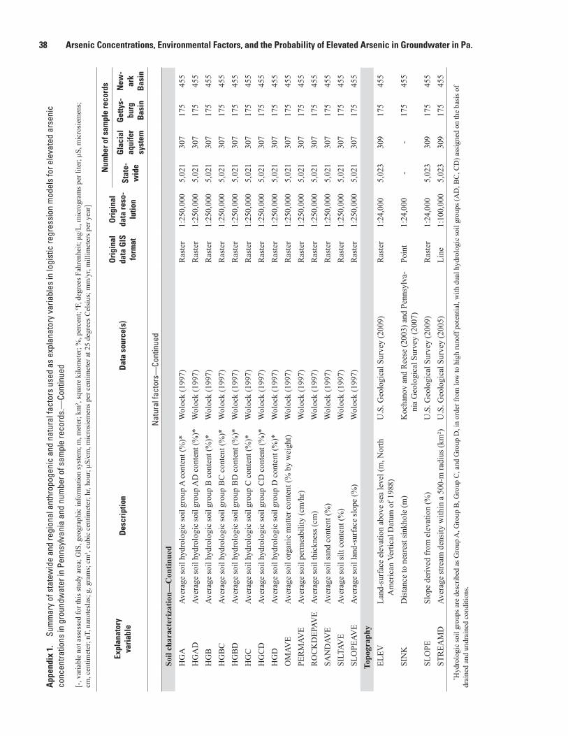
38 Arsenic Concentrations, Environmental Factors, and the Probability of Elevated Arsenic in Groundwater in Pa.A
ppen
dix
1.
Sum
mar
y of
sta
tew
ide
and
regi
onal
ant
hrop
ogen
ic a
nd n
atur
al fa
ctor
s us
ed a
s ex
plan
ator
y va
riabl
es in
logi
stic
regr
essi
on m
odel
s fo
r ele
vate
d ar
seni
c co
ncen
tratio
ns in
gro
undw
ater
in P
enns
ylva
nia
and
num
ber o
f sam
ple
reco
rds.
—Co
ntin
ued
[-, v
aria
ble
not a
sses
sed
for t
his s
tudy
are
a; G
IS, g
eogr
aphi
c in
form
atio
n sy
stem
; m, m
eter
; km
², sq
uare
kilo
met
er; %
, per
cent
; ºF,
deg
rees
Fah
renh
eit;
μg/L
, mic
rogr
ams p
er li
ter;
μS, m
icro
siem
ens;
cm
, cen
timet
er; n
T, n
anot
esla
s; g
, gra
ms;
cm
³, cu
bic
cent
imet
er; h
r, ho
ur; μ
S/cm
, mic
rosi
emen
s per
cen
timet
er a
t 25
degr
ees C
elsi
us; m
m/y
r, m
illim
eter
s per
yea
r]
Expl
anat
ory
vari
able
Des
crip
tion
Dat
a so
urce
(s)
Ori
gina
l da
ta G
IS
form
at
Ori
gina
l da
ta re
so-
lutio
n
Num
ber o
f sam
ple
reco
rds
Stat
e-w
ide
Gla
cial
aq
uife
r sy
stem
Get
tys-
burg
B
asin
New
-ar
k B
asin
Nat
ural
fact
ors—
Cont
inue
d
Soil
char
acte
riza
tion—
Con
tinue
dH
GA
Aver
age
soil
hydr
olog
ic so
il gr
oup
A c
onte
nt (%
)*W
oloc
k (1
997)
Ras
ter
1:25
0,00
05,
021
307
175
455
HG
AD
Aver
age
soil
hydr
olog
ic so
il gr
oup
AD
con
tent
(%)*
Wol
ock
(199
7)R
aste
r1:
250,
000
5,02
130
717
545
5H
GB
Aver
age
soil
hydr
olog
ic so
il gr
oup
B c
onte
nt (%
)*W
oloc
k (1
997)
Ras
ter
1:25
0,00
05,
021
307
175
455
HG
BC
Aver
age
soil
hydr
olog
ic so
il gr
oup
BC
con
tent
(%)*
Wol
ock
(199
7)R
aste
r1:
250,
000
5,02
130
717
545
5H
GB
DAv
erag
e so
il hy
drol
ogic
soil
grou
p B
D c
onte
nt (%
)*W
oloc
k (1
997)
Ras
ter
1:25
0,00
05,
021
307
175
455
HG
CAv
erag
e so
il hy
drol
ogic
soil
grou
p C
con
tent
(%)*
Wol
ock
(199
7)R
aste
r1:
250,
000
5,02
130
717
545
5H
GC
DAv
erag
e so
il hy
drol
ogic
soil
grou
p C
D c
onte
nt (%
)*W
oloc
k (1
997)
Ras
ter
1:25
0,00
05,
021
307
175
455
HG
DAv
erag
e so
il hy
drol
ogic
soil
grou
p D
con
tent
(%)*
Wol
ock
(199
7)R
aste
r1:
250,
000
5,02
130
717
545
5O
MAV
EAv
erag
e so
il or
gani
c m
atte
r con
tent
(% b
y w
eigh
t)W
oloc
k (1
997)
Ras
ter
1:25
0,00
05,
021
307
175
455
PER
MAV
EAv
erag
e so
il pe
rmea
bilit
y (c
m/h
r)W
oloc
k (1
997)
Ras
ter
1:25
0,00
05,
021
307
175
455
RO
CK
DEP
AVE
Aver
age
soil
thic
knes
s (cm
)W
oloc
k (1
997)
Ras
ter
1:25
0,00
05,
021
307
175
455
SAN
DAV
EAv
erag
e so
il sa
nd c
onte
nt (%
)W
oloc
k (1
997)
Ras
ter
1:25
0,00
05,
021
307
175
455
SILT
AVE
Aver
age
soil
silt
cont
ent (
%)
Wol
ock
(199
7)R
aste
r1:
250,
000
5,02
130
717
545
5SL
OPE
AVE
Aver
age
soil
land
-sur
face
slop
e (%
)W
oloc
k (1
997)
Ras
ter
1:25
0,00
05,
021
307
175
455
Topo
grap
hyEL
EVLa
nd-s
urfa
ce e
leva
tion
abov
e se
a le
vel (
m, N
orth
A
mer
ican
Ver
tical
Dat
um o
f 198
8)U
.S. G
eolo
gica
l Sur
vey
(200
9)R
aste
r1:
24,0
005,
023
309
175
455
SIN
KD
ista
nce
to n
eare
st si
nkho
le (m
)K
ocha
nov
and
Ree
se (2
003)
and
Pen
nsyl
va-
nia
Geo
logi
cal S
urve
y (2
007)
Poin
t1:
24,0
00-
-17
545
5
SLO
PESl
ope
deriv
ed fr
om e
leva
tion
(%)
U.S
. Geo
logi
cal S
urve
y (2
009)
Ras
ter
1:24
,000
5,02
330
917
545
5ST
REA
MD
Aver
age
stre
am d
ensi
ty w
ithin
a 5
00-m
radi
us (k
m²)
U.S
. Geo
logi
cal S
urve
y (2
005)
Line
1:10
0,00
05,
023
309
175
455
* Hyd
rolo
gic
soil
grou
ps a
re d
escr
ibed
as G
roup
A, G
roup
B, G
roup
C, a
nd G
roup
D, i
n or
der f
rom
low
to h
igh
runo
ff po
tent
ial,
with
dua
l hyd
rolo
gic
soil
grou
ps (A
D, B
C, C
D) a
ssig
ned
on th
e ba
sis o
f dr
aine
d an
d un
drai
ned
cond
ition
s.

Appendix 2 39
App
endi
x 2.
Su
mm
ary
of a
rsen
ic c
once
ntra
tions
in g
roun
dwat
er (1
969–
2007
) for
the
193
geol
ogic
uni
ts in
Pen
nsyl
vani
a w
ith m
ajor
aqu
ifer t
ype
and
prim
ary
litho
logy
.—Co
ntin
ued
[* in
dica
tes g
eolo
gic
unit
parti
ally
ove
rlain
by
surfi
cial
mat
eria
ls c
onsi
stin
g of
coa
rse
grai
ned
sedi
men
ts (S
olle
r and
Pac
kard
, 199
8; L
inds
ey a
nd B
ickf
ord,
199
9) a
nd th
at so
me
sam
ple
reco
rds a
ssoc
iate
d w
ith
thes
e ge
olog
ic u
nits
may
be
cate
goriz
ed w
ith th
e su
rfici
al m
ajor
aqu
ifer t
ype;
μg/
L, m
icro
gram
s per
lite
r; <,
less
than
; --,
geol
ogic
uni
t with
no
sam
ple
reco
rds]
Maj
or
aqui
fer
type
Prim
ary
litho
logy
¹G
eolo
gic
unit
nam
e¹N
umbe
r of
sam
ple
re
cord
s
Med
ian
ar
seni
c
conc
entr
atio
n,
in μ
g/L
Max
imum
ar
seni
c
conc
entr
atio
n,
in μ
g/L
Num
ber o
f sam
ple
reco
rds
with
ars
enic
co
ncen
trat
ions
gre
ater
th
an o
r equ
al to
4.0
μg/
L
Num
ber o
f sam
ple
reco
rds
with
ars
enic
co
ncen
trat
ions
gre
ater
th
an o
r equ
al to
10.
0 μg
/LC
arbo
nate
Arg
illac
eous
dol
omite
Vin
tage
For
mat
ion
8<4
.0<4
.00
0C
arbo
nate
Arg
illac
eous
lim
esto
neC
ham
bers
burg
For
mat
ion
4<4
.04.
41
0C
arbo
nate
Arg
illac
eous
lim
esto
neH
ersh
ey a
nd M
yers
tow
n Fo
rmat
ions
, und
ivid
ed3
<4.0
12.0
11
Car
bona
teA
rgill
aceo
us li
mes
tone
Her
shey
For
mat
ion
thro
ugh
Ann
ville
For
mat
ion,
und
ivid
ed0
----
00
Car
bona
teA
rgill
aceo
us li
mes
tone
Lim
esto
ne o
f Mar
tinsb
urg
Form
atio
n3
<4.0
8.7
10
Car
bona
teA
rgill
aceo
us li
mes
tone
Plea
sant
Hill
For
mat
ion
1<4
.0<4
.00
0C
arbo
nate
Dol
omite
Alle
ntow
n Fo
rmat
ion
39<4
.010
.04
1C
arbo
nate
Dol
omite
Bel
lefo
nte
and
Axe
man
n Fo
rmat
ions
, und
ivid
ed0
----
00
Car
bona
teD
olom
iteB
elle
font
e Fo
rmat
ion
17<4
.06.
41
0C
arbo
nate
Dol
omite
Gat
esbu
rg F
orm
atio
n7
<4.0
<4.0
00
Car
bona
teD
olom
iteLe
dger
For
mat
ion
54<4
.020
.04
4C
arbo
nate
Dol
omite
Leith
svill
e Fo
rmat
ion
24<4
.040
.01
1C
arbo
nate
Dol
omite
Low
er (M
iddl
e?) C
ambr
ian
rock
s, un
divi
ded
0--
--0
0C
arbo
nate
Dol
omite
Min
es M
embe
r of G
ates
burg
For
mat
ion
8<4
.05.
91
0C
arbo
nate
Dol
omite
Nitt
any
and
Ston
ehen
ge/L
arke
For
mat
ions
, und
ivid
ed12
<4.0
10.0
32
Car
bona
teD
olom
iteN
ittan
y Fo
rmat
ion
7<4
.0<4
.00
0C
arbo
nate
Dol
omite
Ont
elau
nee
Form
atio
n6
<4.0
10.0
21
Car
bona
teD
olom
itePi
nesb
urg
Stat
ion
Form
atio
n6
<4.0
5.0
20
Car
bona
teD
olom
iteR
ichl
and
Form
atio
n3
<4.0
<4.0
00
Car
bona
teD
olom
iteR
icke
nbac
h Fo
rmat
ion
9<4
.0<4
.00
0C
arbo
nate
Dol
omite
Snitz
Cre
ek F
orm
atio
n6
<4.0
<4.0
00
Car
bona
teD
olom
iteTo
mst
own
Form
atio
n7
<4.0
<4.0
00
Car
bona
teD
olom
iteZo
oks C
orne
r For
mat
ion
25<4
.0<4
.00
0C
arbo
nate
Gra
phiti
c m
arbl
eFr
ankl
in M
arbl
e0
----
00
Car
bona
teH
igh-
calc
ium
lim
esto
neA
nnvi
lle F
orm
atio
n0
----
00
Car
bona
teH
igh-
calc
ium
lim
esto
neVa
lent
ine
Mem
ber o
f Ben
ner F
orm
atio
n0
----
00
Car
bona
teLi
mes
tone
Axe
man
n Fo
rmat
ion
6<4
.0<4
.00
0C
arbo
nate
Lim
esto
neB
eekm
anto
wn
Gro
up14
<4.0
40.0
11
Car
bona
teLi
mes
tone
Ben
ner F
orm
atio
n th
roug
h Lo
ysbu
rg F
orm
atio
n, u
ndiv
ided
13<4
.04.
01
0C
arbo
nate
Lim
esto
neB
uffa
lo S
prin
gs F
orm
atio
n12
<4.0
7.0
20
Car
bona
teLi
mes
tone
Cob
urn
Form
atio
n th
roug
h Lo
ysbu
rg F
orm
atio
n, u
ndiv
ided
4<4
.010
.01
1C
arbo
nate
Lim
esto
neC
obur
n Fo
rmat
ion
thro
ugh
Nea
lmon
t For
mat
ion,
und
ivid
ed20
<4.0
<4.0
00
Car
bona
teLi
mes
tone
Con
esto
ga F
orm
atio
n59
<4.0
67.0
63
Car
bona
teLi
mes
tone
Eple
r For
mat
ion
42<4
.05.
03
0C
arbo
nate
Lim
esto
neK
eyse
r and
Ton
olow
ay F
orm
atio
ns, u
ndiv
ided
*46
<4.0
110.
08
4C
arbo
nate
Lim
esto
neK
eyse
r For
mat
ion
thro
ugh
Clin
ton
Gro
up, u
ndiv
ided
0--
--0
0C
arbo
nate
Lim
esto
neK
eyse
r For
mat
ion
thro
ugh
Miffl
into
wn
Form
atio
n, u
ndiv
ided
*9
<4.0
217.
51
1C
arbo
nate
Lim
esto
neLi
mes
tone
of H
ambu
rg se
quen
ce4
<4.0
<4.0
00
Car
bona
teLi
mes
tone
Mill
bach
and
Sch
aeffe
rsto
wn
Form
atio
ns, u
ndiv
ided
2<4
.0<4
.00
0

40 Arsenic Concentrations, Environmental Factors, and the Probability of Elevated Arsenic in Groundwater in Pa.A
ppen
dix
2.
Sum
mar
y of
ars
enic
con
cent
ratio
ns in
gro
undw
ater
(196
9–20
07) f
or th
e 19
3 ge
olog
ic u
nits
in P
enns
ylva
nia
with
maj
or a
quife
r typ
e an
d pr
imar
y lit
holo
gy.—
Cont
inue
d
[* in
dica
tes g
eolo
gic
unit
parti
ally
ove
rlain
by
surfi
cial
mat
eria
ls c
onsi
stin
g of
coa
rse
grai
ned
sedi
men
ts (S
olle
r and
Pac
kard
, 199
8; L
inds
ey a
nd B
ickf
ord,
199
9) a
nd th
at so
me
sam
ple
reco
rds a
ssoc
iate
d w
ith
thes
e ge
olog
ic u
nits
may
be
cate
goriz
ed w
ith th
e su
rfici
al m
ajor
aqu
ifer t
ype;
μg/
L, m
icro
gram
s per
lite
r; <,
less
than
; --,
geol
ogic
uni
t with
no
sam
ple
reco
rds]
Maj
or
aqui
fer
type
Prim
ary
litho
logy
¹G
eolo
gic
unit
nam
e¹N
umbe
r of
sam
ple
re
cord
s
Med
ian
ar
seni
c
conc
entr
atio
n,
in μ
g/L
Max
imum
ar
seni
c
conc
entr
atio
n,
in μ
g/L
Num
ber o
f sam
ple
reco
rds
with
ars
enic
co
ncen
trat
ions
gre
ater
th
an o
r equ
al to
4.0
μg/
L
Num
ber o
f sam
ple
reco
rds
with
ars
enic
co
ncen
trat
ions
gre
ater
th
an o
r equ
al to
10.
0 μg
/LC
arbo
nate
Lim
esto
neM
illba
ch F
orm
atio
n5
<4.0
<4.0
00
Car
bona
teLi
mes
tone
Mon
onga
hela
Gro
up*
19<4
.024
.11
1C
arbo
nate
Lim
esto
neR
ockd
ale
Run
For
mat
ion
16<4
.06.
11
0C
arbo
nate
Lim
esto
neSh
adyg
rove
For
mat
ion
6<4
.0<4
.00
0C
arbo
nate
Lim
esto
neSh
river
, Man
data
, Cor
rigan
ville
, and
New
Cre
ek M
embe
rs o
f Old
Por
t For
mat
ion,
und
ivid
ed0
----
00
Car
bona
teLi
mes
tone
Snitz
Cre
ek a
nd B
uffa
lo S
prin
gs F
orm
atio
ns, u
ndiv
ided
4<4
.0<4
.00
0C
arbo
nate
Lim
esto
neSt
. Pau
l Gro
up9
<4.0
<4.0
00
Car
bona
teLi
mes
tone
Ston
ehen
ge F
orm
atio
n29
<4.0
5.8
30
Car
bona
teLi
mes
tone
Ston
ehen
ge/L
arke
For
mat
ion
4<4
.08.
81
0C
arbo
nate
Lim
esto
neW
arrio
r For
mat
ion
2<4
.0<4
.00
0C
arbo
nate
Lim
esto
neZu
lling
er F
orm
atio
n7
<4.0
<4.0
00
Car
bona
teLi
mes
tone
con
glom
erat
eLi
mes
tone
fang
lom
erat
e7
<4.0
4.3
10
Car
bona
teM
arbl
eC
ocke
ysvi
lle M
arbl
e19
<4.0
<4.0
00
Car
bona
teM
arbl
eW
akefi
eld
Mar
ble
0--
--0
0C
arbo
nate
Shal
y lim
esto
neJa
ckso
nbur
g Fo
rmat
ion
86.
220
.75
2C
ryst
allin
eA
lbite
-chl
orite
schi
stO
ctor
aro
Form
atio
n66
<4.0
10.0
32
Cry
stal
line
And
esite
Jone
stow
n Vo
lcan
ic S
uite
3<4
.0<4
.00
0C
ryst
allin
eA
north
osite
Ano
rthos
ite7
<4.0
<4.0
00
Cry
stal
line
Chl
orite
-ser
icite
schi
stPe
ters
Cre
ek S
chis
t47
<4.0
7.0
30
Cry
stal
line
Dia
base
Dia
base
92<4
.060
.017
7C
ryst
allin
eFe
ldsp
athi
c qu
artz
iteSe
tters
Qua
rtzite
28<4
.06.
11
0C
ryst
allin
eFe
lsic
gne
iss
Fels
ic a
nd in
term
edia
te g
neis
s10
6<4
.0<4
.00
0C
ryst
allin
eFe
lsic
gne
iss
Fels
ic g
neis
s34
<4.0
23.9
21
Cry
stal
line
Fels
ic g
neis
sFe
lsic
to m
afic
gnei
ss58
<4.0
20.0
41
Cry
stal
line
Gra
nitic
gne
iss
Gra
nitic
gne
iss a
nd g
rani
te0
----
00
Cry
stal
line
Gra
nitic
peg
mat
itePe
gmat
ite1
<4.0
<4.0
00
Cry
stal
line
Gra
phiti
c fe
lsic
gne
iss
Gra
phiti
c fe
lsic
gne
iss
18<4
.0<4
.00
0C
ryst
allin
eG
raph
itic
gnei
ssG
raph
itic
fels
ic g
neis
s28
<4.0
5.0
20
Cry
stal
line
Gre
enst
one
schi
stG
reen
ston
e sc
hist
0--
--0
0C
ryst
allin
eM
afic
gnei
ssB
ande
d m
afic
gnei
ss16
<4.0
<4.0
00
Cry
stal
line
Mafi
c gn
eiss
Hor
nble
nde
gnei
ss21
<4.0
20.0
62
Cry
stal
line
Mafi
c gn
eiss
Mafi
c gn
eiss
15<4
.0<4
.00
0C
ryst
allin
eM
etab
asal
tM
etab
asal
t1
<4.0
<4.0
00
Cry
stal
line
Met
abas
alt
Sam
s Cre
ek M
etab
asal
t2
<4.0
<4.0
00
Cry
stal
line
Met
adia
base
Met
adia
base
0--
--0
0C
ryst
allin
eM
etag
abbr
oM
etag
abbr
o0
----
00
Cry
stal
line
Met
arhy
olite
Met
arhy
olite
5<4
.0<4
.00
0C
ryst
allin
eO
ligoc
lase
-mic
a sc
hist
Gle
narm
Wis
sahi
ckon
form
atio
n13
4<4
.04.
01
0C
ryst
allin
eO
ligoc
lase
-mic
a sc
hist
Wis
sahi
ckon
For
mat
ion
28<4
.04.
01
0
Appendix 2 41
App
endi
x 2.
Su
mm
ary
of a
rsen
ic c
once
ntra
tions
in g
roun
dwat
er (1
969–
2007
) for
the
193
geol
ogic
uni
ts in
Pen
nsyl
vani
a w
ith m
ajor
aqu
ifer t
ype
and
prim
ary
litho
logy
.—Co
ntin
ued
[* in
dica
tes g
eolo
gic
unit
parti
ally
ove
rlain
by
surfi
cial
mat
eria
ls c
onsi
stin
g of
coa
rse
grai
ned
sedi
men
ts (S
olle
r and
Pac
kard
, 199
8; L
inds
ey a
nd B
ickf
ord,
199
9) a
nd th
at so
me
sam
ple
reco
rds a
ssoc
iate
d w
ith
thes
e ge
olog
ic u
nits
may
be
cate
goriz
ed w
ith th
e su
rfici
al m
ajor
aqu
ifer t
ype;
μg/
L, m
icro
gram
s per
lite
r; <,
less
than
; --,
geol
ogic
uni
t with
no
sam
ple
reco
rds]
Maj
or
aqui
fer
type
Prim
ary
litho
logy
¹G
eolo
gic
unit
nam
e¹N
umbe
r of
sam
ple
re
cord
s
Med
ian
ar
seni
c
conc
entr
atio
n,
in μ
g/L
Max
imum
ar
seni
c
conc
entr
atio
n,
in μ
g/L
Num
ber o
f sam
ple
reco
rds
with
ars
enic
co
ncen
trat
ions
gre
ater
th
an o
r equ
al to
4.0
μg/
L
Num
ber o
f sam
ple
reco
rds
with
ars
enic
co
ncen
trat
ions
gre
ater
th
an o
r equ
al to
10.
0 μg
/LC
ryst
allin
ePh
yllit
eH
arpe
rs F
orm
atio
n1
<4.0
<4.0
00
Cry
stal
line
Phyl
lite
Mar
burg
Sch
ist
16<4
.0<4
.00
0C
ryst
allin
eQ
uartz
iteA
ntie
tam
and
Har
pers
For
mat
ions
, und
ivid
ed24
<4.0
10.0
11
Cry
stal
line
Qua
rtzite
Ant
ieta
m F
orm
atio
n2
<4.0
<4.0
00
Cry
stal
line
Qua
rtzite
Chi
ckie
s For
mat
ion
55<4
.040
.09
3C
ryst
allin
eQ
uartz
iteH
ardy
ston
For
mat
ion
14<4
.020
.03
3C
ryst
allin
eQ
uartz
iteM
onta
lto M
embe
r of H
arpe
rs F
orm
atio
n1
<4.0
<4.0
00
Cry
stal
line
Qua
rtzite
Wev
erto
n an
d Lo
udou
n Fo
rmat
ions
, und
ivid
ed0
----
00
Cry
stal
line
Serp
entin
iteU
ltram
afic
rock
s27
<4.0
<4.0
00
Cry
stal
line
Slat
ePe
ach
Bot
tom
Sla
te a
nd C
ardi
ff C
ongl
omer
ate,
und
ivid
ed2
<4.0
10.0
11
Silic
icla
stic
Arg
illac
eous
sand
ston
eR
ockw
ell F
orm
atio
n1
<4.0
<4.0
00
Silic
icla
stic
Arg
illac
eous
shal
eG
irard
Sha
le*
41<4
.029
3.0
164
Silic
icla
stic
Arg
illite
Lock
aton
g Fo
rmat
ion
54<4
.040
.019
4Si
licic
last
icA
rkos
ic sa
ndst
one
New
Oxf
ord
Form
atio
n45
<4.0
85.5
1510
Silic
icla
stic
Ark
osic
sand
ston
eSe
dim
enta
ry st
rata
at J
acks
onw
ald
and
Asp
ers
0--
--0
0Si
licic
last
icA
rkos
ic sa
ndst
one
Stoc
kton
For
mat
ion
141
<4.0
69.0
234
Silic
icla
stic
Bla
ck sh
ale
Mar
cellu
s For
mat
ion*
4<4
.07.
01
0Si
licic
last
icC
alca
reou
s san
dsto
neD
ecke
r For
mat
ion
thro
ugh
Poxo
no Is
land
For
mat
ion,
und
ivid
ed*
2<4
.0<4
.00
0Si
licic
last
icC
alca
reou
s sha
leEl
broo
k Fo
rmat
ion
25<4
.0<4
.00
0Si
licic
last
icC
alca
reou
s sha
leO
nond
aga
and
Old
Por
t For
mat
ions
, und
ivid
ed*
37<4
.020
.05
2Si
licic
last
icC
alca
reou
s sha
leO
nond
aga
Form
atio
n1
<4.0
<4.0
00
Silic
icla
stic
Cal
care
ous s
hale
Will
s Cre
ek F
orm
atio
n th
roug
h M
ifflin
tow
n Fo
rmat
ion,
und
ivid
ed2
<4.0
<4.0
00
Silic
icla
stic
Cal
care
ous s
hale
Will
s Cre
ek F
orm
atio
n*36
<4.0
22.0
61
Silic
icla
stic
Gra
ywac
keG
rayw
acke
and
shal
e of
Mar
tinsb
urg
Form
atio
n22
<4.0
20.0
71
Silic
icla
stic
Gra
ywac
keG
rayw
acke
of H
ambu
rg se
quen
ce10
<4.0
<4.0
00
Silic
icla
stic
Mud
ston
eB
runs
wic
k Fo
rmat
ion
257
<4.0
60.9
104
43Si
licic
last
icM
udst
one
Lock
Hav
en F
orm
atio
n*19
7<4
.017
8.0
5930
Silic
icla
stic
Mud
ston
eSh
erm
an C
reek
Mem
ber o
f Cat
skill
For
mat
ion*
474.
049
.824
12Si
licic
last
icQ
uartz
con
glom
erat
eG
etty
sbur
g co
nglo
mer
ate
6<4
.0<4
.00
0Si
licic
last
icQ
uartz
con
glom
erat
eH
amm
er C
reek
con
glom
erat
e19
<4.0
7.6
40
Silic
icla
stic
Qua
rtz c
ongl
omer
ate
New
Oxf
ord
cong
lom
erat
e3
<4.0
<4.0
00
Silic
icla
stic
Qua
rtz c
ongl
omer
ate
Qua
rtz fa
nglo
mer
ate
10<4
.013
.62
1Si
licic
last
icQ
uartz
con
glom
erat
eSt
ockt
on c
ongl
omer
ate
0--
--0
0Si
licic
last
icQ
uartz
iteTu
scar
ora
Form
atio
n*1
<4.0
<4.0
00
Silic
icla
stic
Sand
ston
eA
llegh
eny
and
Potts
ville
For
mat
ions
, und
ivid
ed*
1<4
.0<4
.00
0Si
licic
last
icSa
ndst
one
Alle
ghen
y Fo
rmat
ion*
233
<4.0
490.
030
12Si
licic
last
icSa
ndst
one
Bal
d Ea
gle
Form
atio
n8
<4.0
6.0
20
Silic
icla
stic
Sand
ston
eB
erea
San
dsto
ne th
roug
h R
icev
ille
Form
atio
n, u
ndiv
ided
*8
<4.0
180.
02
1Si
licic
last
icSa
ndst
one
Ber
ea S
ands
tone
thro
ugh
Vena
ngo
Form
atio
n, u
ndiv
ided
*17
16.0
58.0
1410

42 Arsenic Concentrations, Environmental Factors, and the Probability of Elevated Arsenic in Groundwater in Pa.A
ppen
dix
2.
Sum
mar
y of
ars
enic
con
cent
ratio
ns in
gro
undw
ater
(196
9–20
07) f
or th
e 19
3 ge
olog
ic u
nits
in P
enns
ylva
nia
with
maj
or a
quife
r typ
e an
d pr
imar
y lit
holo
gy.—
Cont
inue
d
[* in
dica
tes g
eolo
gic
unit
parti
ally
ove
rlain
by
surfi
cial
mat
eria
ls c
onsi
stin
g of
coa
rse
grai
ned
sedi
men
ts (S
olle
r and
Pac
kard
, 199
8; L
inds
ey a
nd B
ickf
ord,
199
9) a
nd th
at so
me
sam
ple
reco
rds a
ssoc
iate
d w
ith
thes
e ge
olog
ic u
nits
may
be
cate
goriz
ed w
ith th
e su
rfici
al m
ajor
aqu
ifer t
ype;
μg/
L, m
icro
gram
s per
lite
r; <,
less
than
; --,
geol
ogic
uni
t with
no
sam
ple
reco
rds]
Maj
or
aqui
fer
type
Prim
ary
litho
logy
¹G
eolo
gic
unit
nam
e¹N
umbe
r of
sam
ple
re
cord
s
Med
ian
ar
seni
c
conc
entr
atio
n,
in μ
g/L
Max
imum
ar
seni
c
conc
entr
atio
n,
in μ
g/L
Num
ber o
f sam
ple
reco
rds
with
ars
enic
co
ncen
trat
ions
gre
ater
th
an o
r equ
al to
4.0
μg/
L
Num
ber o
f sam
ple
reco
rds
with
ars
enic
co
ncen
trat
ions
gre
ater
th
an o
r equ
al to
10.
0 μg
/LSi
licic
last
icSa
ndst
one
Ber
ry R
un a
nd S
awm
ill R
un M
embe
rs o
f Cat
skill
For
mat
ion,
und
ivid
ed0
----
00
Silic
icla
stic
Sand
ston
eB
urgo
on S
ands
tone
thro
ugh
Cuy
ahog
a G
roup
, und
iffer
entia
ted*
14.
04.
01
0Si
licic
last
icSa
ndst
one
Bur
goon
San
dsto
ne*
19<4
.09.
33
0Si
licic
last
icSa
ndst
one
Cat
skill
For
mat
ion*
247
<4.0
188.
082
37Si
licic
last
icSa
ndst
one
Cla
rks F
erry
Mem
ber o
f Cat
skill
For
mat
ion
0--
--0
0Si
licic
last
icSa
ndst
one
Cor
ry S
ands
tone
thro
ugh
Ric
evill
e Fo
rmat
ion,
und
ivid
ed*
28<4
.064
.45
3Si
licic
last
icSa
ndst
one
Dun
cann
on M
embe
r of C
atsk
ill F
orm
atio
n*20
<4.0
4.0
10
Silic
icla
stic
Sand
ston
eFo
rekn
obs F
orm
atio
n15
6.3
12.6
83
Silic
icla
stic
Sand
ston
eG
reen
e Fo
rmat
ion
7<4
.010
.02
1Si
licic
last
icSa
ndst
one
Ham
mer
Cre
ek F
orm
atio
n43
<4.0
20.7
83
Silic
icla
stic
Sand
ston
eH
untle
y M
ount
ain
Form
atio
n*30
<4.0
10.0
141
Silic
icla
stic
Sand
ston
eJu
niat
a an
d B
ald
Eagl
e Fo
rmat
ions
, und
ivid
ed1
<4.0
<4.0
00
Silic
icla
stic
Sand
ston
eJu
niat
a Fo
rmat
ion
9<4
.010
.03
1Si
licic
last
icSa
ndst
one
Llew
elly
n Fo
rmat
ion*
20<4
.011
.42
1Si
licic
last
icSa
ndst
one
Long
Run
and
Wal
cksv
ille
Mem
bers
of C
atsk
ill F
orm
atio
n, u
ndiv
ided
*43
<4.0
15.0
71
Silic
icla
stic
Sand
ston
eLo
ng R
un M
embe
r of C
atsk
ill F
orm
atio
n*7
<4.0
10.0
21
Silic
icla
stic
Sand
ston
eLo
wer
mem
bers
of G
ates
burg
For
mat
ion,
und
ivid
ed2
<4.0
<4.0
00
Silic
icla
stic
Sand
ston
ePa
cker
ton
Mem
ber o
f Cat
skill
For
mat
ion
0--
--0
0Si
licic
last
icSa
ndst
one
Poco
no a
nd R
ockw
ell F
orm
atio
ns, u
ndiv
ided
0--
--0
0Si
licic
last
icSa
ndst
one
Poco
no F
orm
atio
n*5
<4.0
<4.0
00
Silic
icla
stic
Sand
ston
ePo
plar
Gap
and
Pac
kerto
n M
embe
rs o
f Cat
skill
For
mat
ion,
und
ivid
ed18
<4.0
20.0
31
Silic
icla
stic
Sand
ston
ePo
plar
Gap
Mem
ber o
f Cat
skill
For
mat
ion
4<4
.010
.01
1Si
licic
last
icSa
ndst
one
Potts
ville
For
mat
ion*
89<4
.021
0.0
2311
Silic
icla
stic
Sand
ston
eR
idge
ley
Form
atio
n th
roug
h C
oeym
ans F
orm
atio
n, u
ndiv
ided
*0
----
00
Silic
icla
stic
Sand
ston
eR
idge
ley
Mem
ber o
f Old
Por
t For
mat
ion
0--
--0
0Si
licic
last
icSa
ndst
one
Shaw
angu
nk F
orm
atio
n*0
----
00
Silic
icla
stic
Sand
ston
eSh
enan
go F
orm
atio
n th
roug
h C
uyah
oga
Gro
up, u
ndiv
ided
*11
<4.0
4.0
10
Silic
icla
stic
Sand
ston
eSh
enan
go F
orm
atio
n th
roug
h O
sway
o Fo
rmat
ion,
und
ivid
ed*
7<4
.06.
01
0Si
licic
last
icSa
ndst
one
Shen
ango
For
mat
ion
thro
ugh
Ric
evill
e Fo
rmat
ion,
und
ivid
ed*
13<4
.017
.05
3Si
licic
last
icSa
ndst
one
Shen
ango
For
mat
ion*
8<4
.011
.02
2Si
licic
last
icSa
ndst
one
Spec
hty
Kop
f For
mat
ion*
2<4
.0<4
.00
0Si
licic
last
icSa
ndst
one
Tow
amen
sing
Mem
ber o
f Cat
skill
For
mat
ion*
8<4
.0<4
.00
0Si
licic
last
icSa
ndst
one
Wal
cksv
ille
and
Tow
amen
sing
Mem
bers
of C
atsk
ill F
orm
atio
n, u
ndiv
ided
2<4
.0<4
.00
0Si
licic
last
icSa
ndst
one
Wal
cksv
ille
Mem
ber o
f Cat
skill
For
mat
ion*
2<4
.04.
01
0Si
licic
last
icSa
ndst
one
Was
hing
ton
Form
atio
n*14
<4.0
6.0
30
Silic
icla
stic
Sand
ston
eW
ayne
sbur
g Fo
rmat
ion*
16<4
.021
.04
2Si
licic
last
icSh
ale
Blo
omsb
urg
and
Miffl
into
wn
Form
atio
ns, u
ndiv
ided
*37
<4.0
57.0
188
Silic
icla
stic
Shal
eB
loom
sbur
g Fo
rmat
ion*
24.
34.
72
0Si
licic
last
icSh
ale
Cas
selm
an F
orm
atio
n*13
6<4
.09.
05
0

Appendix 2 43
App
endi
x 2.
Su
mm
ary
of a
rsen
ic c
once
ntra
tions
in g
roun
dwat
er (1
969–
2007
) for
the
193
geol
ogic
uni
ts in
Pen
nsyl
vani
a w
ith m
ajor
aqu
ifer t
ype
and
prim
ary
litho
logy
.—Co
ntin
ued
[* in
dica
tes g
eolo
gic
unit
parti
ally
ove
rlain
by
surfi
cial
mat
eria
ls c
onsi
stin
g of
coa
rse
grai
ned
sedi
men
ts (S
olle
r and
Pac
kard
, 199
8; L
inds
ey a
nd B
ickf
ord,
199
9) a
nd th
at so
me
sam
ple
reco
rds a
ssoc
iate
d w
ith
thes
e ge
olog
ic u
nits
may
be
cate
goriz
ed w
ith th
e su
rfici
al m
ajor
aqu
ifer t
ype;
μg/
L, m
icro
gram
s per
lite
r; <,
less
than
; --,
geol
ogic
uni
t with
no
sam
ple
reco
rds]
Maj
or
aqui
fer
type
Prim
ary
litho
logy
¹G
eolo
gic
unit
nam
e¹N
umbe
r of
sam
ple
re
cord
s
Med
ian
ar
seni
c
conc
entr
atio
n,
in μ
g/L
Max
imum
ar
seni
c
conc
entr
atio
n,
in μ
g/L
Num
ber o
f sam
ple
reco
rds
with
ars
enic
co
ncen
trat
ions
gre
ater
th
an o
r equ
al to
4.0
μg/
L
Num
ber o
f sam
ple
reco
rds
with
ars
enic
co
ncen
trat
ions
gre
ater
th
an o
r equ
al to
10.
0 μg
/LSi
licic
last
icSh
ale
Clin
ton
Gro
up*
25<4
.07.
04
0Si
licic
last
icSh
ale
Coc
alic
o Fo
rmat
ion
20<4
.030
.55
1Si
licic
last
icSh
ale
Con
emau
gh G
roup
7<4
.0<4
.00
0Si
licic
last
icSh
ale
Gle
nsha
w F
orm
atio
n*42
6<4
.020
0.0
2011
Silic
icla
stic
Shal
eH
ambu
rg se
quen
ce ro
cks
86<4
.012
.08
1Si
licic
last
icSh
ale
Ham
ilton
Gro
up*
109
<4.0
28.0
184
Silic
icla
stic
Shal
eH
eidl
ersb
urg
Mem
ber o
f Get
tysb
urg
Form
atio
n6
<4.0
6.0
10
Silic
icla
stic
Shal
eK
inze
rs F
orm
atio
n9
<4.0
<4.0
00
Silic
icla
stic
Shal
eM
ahan
tang
o Fo
rmat
ion*
18<4
.04.
52
0Si
licic
last
icSh
ale
Mar
tinsb
urg
Form
atio
n10
7<4
.016
1.0
169
Silic
icla
stic
Shal
eM
auch
Chu
nk F
orm
atio
n*91
<4.0
230.
016
7Si
licic
last
icSh
ale
Nor
thea
st S
hale
*3
<4.0
<4.0
00
Silic
icla
stic
Shal
eO
nond
aga
Form
atio
n th
roug
h Po
xono
Isla
nd F
orm
atio
n, u
ndiv
ided
0--
--0
0Si
licic
last
icSh
ale
Ree
dsvi
lle F
orm
atio
n21
<4.0
4.2
20
Silic
icla
stic
Shal
eSh
ale
and
gray
wac
ke o
f Ham
burg
sequ
ence
31<4
.020
.04
2Si
licic
last
icSh
ale
Way
nesb
oro
Form
atio
n5
<4.0
<4.0
00
Silic
icla
stic
Silic
eous
sand
ston
eB
utte
rmilk
Fal
ls L
imes
tone
thro
ugh
Esop
us F
orm
atio
n, u
ndiv
ided
*1
<4.0
<4.0
00
Silic
icla
stic
Silts
tone
Bea
verd
am R
un M
embe
r of C
atsk
ill F
orm
atio
n*2
4.5
5.0
20
Silic
icla
stic
Silts
tone
Bra
llier
and
Har
rell
Form
atio
ns, u
ndiv
ided
*15
<4.0
23.0
31
Silic
icla
stic
Silts
tone
Bud
dys R
un M
embe
r of C
atsk
ill F
orm
atio
n*11
<4.0
19.0
41
Silic
icla
stic
Silts
tone
Cha
dako
in F
orm
atio
n*12
9<4
.023
0.0
4932
Silic
icla
stic
Silts
tone
Cuy
ahog
a G
roup
*8
<4.0
21.0
31
Silic
icla
stic
Silts
tone
Iris
h Va
lley
Mem
ber o
f Cat
skill
For
mat
ion*
20<4
.085
.05
2Si
licic
last
icSi
ltsto
neSc
herr
For
mat
ion
8<4
.05.
02
0Si
licic
last
icSi
ltsto
neTr
imm
ers R
ock
Form
atio
n*72
<4.0
7.0
60
Silic
icla
stic
Silts
tone
Vena
ngo
Form
atio
n*11
7<4
.068
.031
19Si
licic
last
icSi
lty m
udst
one
Get
tysb
urg
Form
atio
n47
<4.0
14.0
143
Surfi
cial
Feld
spat
hic
quar
tz sa
ndPe
nsau
ken
and
Brid
geto
n Fo
rmat
ions
, und
iffer
entia
ted
3<4
.011
.01
1Su
rfici
alFe
rrug
inou
s cla
yPa
taps
co(?
) For
mat
ion
0--
--0
0Su
rfici
alG
rave
lly sa
ndB
ryn
Maw
r For
mat
ion
0--
--0
0Su
rfici
alG
rave
lly sa
ndTr
ento
n G
rave
l38
<4.0
50.0
169
Surfi
cial
Sand
Sand
s of P
resq
ue Is
le27
103.
021
6.0
2727
1 Dat
a fr
om P
enns
ylva
nia
Geo
logi
cal S
urve
y, 2
001.

44 Arsenic Concentrations, Environmental Factors, and the Probability of Elevated Arsenic in Groundwater in Pa.A
ppen
dix
3.
Resu
lts o
f uni
varia
te lo
gist
ic re
gres
sion
ana
lyse
s w
ith lo
gist
ic re
gres
sion
sta
ndar
dize
d co
effic
ient
s an
d in
divi
dual
p-v
alue
s of
inde
pend
ent v
aria
bles
rela
ted
to
the
dete
ctio
n of
ele
vate
d co
ncen
tratio
ns o
f ars
enic
in g
roun
dwat
er s
ampl
es c
olle
cted
sta
tew
ide
and
in th
ree
regi
ons
in P
enns
ylva
nia.
—Co
ntin
ued
[NS,
var
iabl
e no
t sel
ecte
d fo
r mul
tivar
iate
ana
lysi
s; --
, var
iabl
e no
t ass
esse
d fo
r thi
s stu
dy a
rea;
<, l
ess t
han;
val
ues n
ot e
nclo
sed
in p
aren
thes
es a
re lo
gist
ic re
gres
sion
stan
dard
ized
coe
ffici
ents
; val
ues
encl
osed
in p
aren
thes
es a
re p
-val
ues;
m, m
eter
; km
², sq
uare
kilo
met
er; %
, per
cent
; ºF,
deg
rees
Fah
renh
eit;
μg/L
, mic
rogr
ams p
er li
ter;
μS, m
icro
siem
ens;
cm
, cen
timet
er; μ
S/cm
, mic
rosi
emen
s per
cen
timet
er
at 2
5 de
gree
s Cel
sius
; nT,
nan
otes
las;
g, g
ram
s; c
m³,
cubi
c ce
ntim
eter
; mm
/yr,
mill
imet
ers p
er y
ear;
hr, h
our]
Expl
anat
ory
va
riab
leD
escr
iptio
nU
niva
riat
e lo
gist
ic re
gres
sion
resu
lts
Stat
ewid
eG
laci
al a
quife
r sy
stem
Get
tysb
urg
Bas
inN
ewar
k
Bas
inAn
thro
poge
nic
fact
ors
MU
ND
ista
nce
to m
unic
ipal
ities
con
tain
ing
wat
er su
pplie
rs w
ith a
rsen
ic tr
eatm
ent a
nd si
tes o
r gro
undw
ater
in
need
of r
emed
iatio
n be
caus
e of
ars
enic
con
tam
inat
ion
(m)
-0.0
505
(0
.016
0)-0
.129
7
(0.0
755)
0.27
47
(0.0
057)
-0.2
951
(<
0.00
01)
TRI
Dis
tanc
e to
toxi
c ch
emic
al re
leas
e in
vent
ory
site
s (m
)N
S-0
.310
7
(0.0
006)
-0.2
893
(0
.010
0)N
S
CO
AL
Dis
tanc
e to
und
ergr
ound
and
surf
ace
coal
min
ing
oper
atio
ns (m
)--
NS
----
IND
MIN
Dis
tanc
e to
indu
stria
l min
eral
min
ing
oper
atio
ns (m
)-0
.054
0
(0.0
106)
0.39
67
(<0.
0001
)N
SN
S
OIL
GA
SD
ista
nce
to o
il an
d ga
s loc
atio
ns (m
)--
-0.3
066
(0
.006
8)--
--
AG
AVE
Aver
age
agric
ultu
ral l
and
cove
r with
in a
500
-m ra
dius
(%)
-0.1
037
(<
0.00
01)
-0.2
530
(0
.000
6)-0
.150
2
(0.1
332)
0.10
44
(0.0
619)
POP
Popu
latio
n de
nsity
(peo
ple/
km²)
NS
NS
0.18
73
(0.0
365)
NS
UR
BAV
EAv
erag
e ur
ban
land
cov
er w
ithin
a 5
00-m
radi
us (%
)0.
0571
(0
.002
8)N
S0.
4095
(<
0.00
01)
NS
Nat
ural
fact
ors
PRE
Aver
age
prec
ipita
tion
from
197
1–20
00 (m
m/y
r)-0
.107
3
(<0.
0001
)N
S-0
.190
5
(0.0
619)
NS
REC
HAv
erag
e gr
ound
wat
er re
char
ge fr
om 1
951–
1980
(mm
/yr)
-0.1
292
(<
0.00
01)
NS
NS
NS
TEM
PAv
erag
e te
mpe
ratu
re fr
om 1
971–
2000
(ºF)
-0.1
066
(<
0.00
01)
0.23
91
(0.0
006)
0.29
50
(0.0
061)
-0.1
130
(0
.042
3)
AC
IDD
ista
nce
to g
eolo
gic
units
con
tain
ing
acid
-pro
duci
ng su
lfide
min
eral
s (m
)0.
1041
(<
0.00
01)
0.43
06
(<0.
0001
)--
0.10
99
(0.0
451)
CA
RB
Car
bona
te m
ajor
aqu
ifer t
ype
(1 =
car
bona
te, 0
= a
ll ot
her)
-0.1
647
(<
0.00
01)
----
--
CRY
STC
ryst
allin
e m
ajor
aqu
ifer t
ype
(1 =
cry
stal
line,
0 =
all
othe
r)-0
.276
8
(<0.
0001
)--
----
DIA
Dis
tanc
e to
dia
base
geo
logi
c un
its (m
)--
--0.
2645
(0
.003
9)-0
.146
0
(0.0
133)
PLU
TIG
Dis
tanc
e to
igne
ous r
ock
loca
tions
(m)
----
NS
-0.1
999
(0
.000
9)
SIL
Silic
icla
stic
maj
or a
quife
r typ
e (1
= si
licic
last
ic, 0
= a
ll ot
her)
0.13
44
(<0.
0001
)--
----

Appendix 3 45A
ppen
dix
3.
Resu
lts o
f uni
varia
te lo
gist
ic re
gres
sion
ana
lyse
s w
ith lo
gist
ic re
gres
sion
sta
ndar
dize
d co
effic
ient
s an
d in
divi
dual
p-v
alue
s of
inde
pend
ent v
aria
bles
rela
ted
to
the
dete
ctio
n of
ele
vate
d co
ncen
tratio
ns o
f ars
enic
in g
roun
dwat
er s
ampl
es c
olle
cted
sta
tew
ide
and
in th
ree
regi
ons
in P
enns
ylva
nia.
—Co
ntin
ued
[NS,
var
iabl
e no
t sel
ecte
d fo
r mul
tivar
iate
ana
lysi
s; --
, var
iabl
e no
t ass
esse
d fo
r thi
s stu
dy a
rea;
<, l
ess t
han;
val
ues n
ot e
nclo
sed
in p
aren
thes
es a
re lo
gist
ic re
gres
sion
stan
dard
ized
coe
ffici
ents
; val
ues
encl
osed
in p
aren
thes
es a
re p
-val
ues;
m, m
eter
; km
², sq
uare
kilo
met
er; %
, per
cent
; ºF,
deg
rees
Fah
renh
eit;
μg/L
, mic
rogr
ams p
er li
ter;
μS, m
icro
siem
ens;
cm
, cen
timet
er; μ
S/cm
, mic
rosi
emen
s per
cen
timet
er
at 2
5 de
gree
s Cel
sius
; nT,
nan
otes
las;
g, g
ram
s; c
m³,
cubi
c ce
ntim
eter
; mm
/yr,
mill
imet
ers p
er y
ear;
hr, h
our]
Expl
anat
ory
va
riab
leD
escr
iptio
nU
niva
riat
e lo
gist
ic re
gres
sion
resu
lts
Stat
ewid
eG
laci
al a
quife
r sy
stem
Get
tysb
urg
Bas
inN
ewar
k
Bas
in
SUR
FSu
rfici
al m
ajor
aqu
ifer t
ype
(1 =
surfi
cial
, 0 =
all
othe
r)0.
1509
(<
0.00
01)
----
--
MA
GAv
erag
e re
sidu
al to
tal i
nten
sity
of t
he e
arth
’s m
agne
tic fi
eld
(nT)
NS
-0.1
232
(0
.096
3)-0
.172
3
(0.1
119)
0.14
18
(0.0
093)
CO
RR
Gro
upin
g of
geo
logi
c un
its a
ccor
ding
to e
stim
ated
gro
undw
ater
cor
rosi
vity
(1 to
11
base
d on
Lan
gelie
r Sa
tura
tion
Inde
x)0.
0805
(0
.000
1)-0
.354
6
(<0.
0001
)0.
2126
(0
.042
2)0.
2975
(<
0.00
01)
NU
REA
SEs
timat
ed a
rsen
ic c
once
ntra
tion
deriv
ed fr
om st
ream
sedi
men
t dat
a (μ
g/L)
----
--0.
1056
(0
.055
0)
PHID
WEs
timat
ed g
roun
dwat
er p
H0.
1283
(<
0.00
01)
--0.
3748
(0
.001
6)0.
3500
(<
0.00
01)
PHID
WG
LAC
Estim
ated
gro
undw
ater
pH
usi
ng o
nly
glac
ial d
ata
--0.
2958
(0
.000
2)--
--
SPC
IDW
Estim
ated
gro
undw
ater
spec
ific
cond
ucta
nce
(μS/
cm)
0.17
52
(<0.
0001
)--
0.36
19
(0.0
006)
0.36
24
(0.0
037)
SPC
IDW
GLA
CEs
timat
ed g
roun
dwat
er sp
ecifi
c co
nduc
tanc
e us
ing
only
gla
cial
dat
a (μ
S/cm
)--
0.52
50
(<0.
0001
)--
--
FOR
AVE
Aver
age
fore
sted
land
cov
er w
ithin
a 5
00-m
radi
us (%
)N
S-0
.243
9
(0.0
013)
-0.2
359
(0
.033
7)-0
.074
0
(0.1
908)
WET
AVE
Aver
age
wet
land
s lan
d co
ver w
ithin
a 5
00-m
radi
us (%
)0.
1409
(<
0.00
01)
0.52
17
(<0.
0001
)N
S0.
1171
(0
.041
4)
MET
MIN
Dis
tanc
e to
met
allic
min
eral
reso
urce
s (m
)0.
0700
(0
.000
3)-0
.237
1
(0.0
012)
0.18
25
(0.0
674)
NS
MIN
Dis
tanc
e to
met
allic
and
non
met
allic
min
eral
reso
urce
s (m
)N
S-0
.135
4
(0.0
727)
NS
NS
NO
NM
ETM
IND
ista
nce
to n
onm
etal
lic m
iner
al re
sour
ces (
m)
NS
NS
-0.1
620
(0
.133
5)N
S
AWC
AVE
Aver
age
soil
avai
labl
e w
ater
cap
acity
(%)
-0.2
133
(<
0.00
01)
-0.2
979
(0
.000
3)N
S-0
.202
8
(0.0
015)
BD
AVE
Aver
age
soil
bulk
den
sity
(g/c
m³)
0.12
68
(0.0
001)
0.52
96
(0.0
001)
NS
NS
CLA
YAV
EAv
erag
e so
il cl
ay c
onte
nt (%
)-0
.242
1
(<0.
0001
)-0
.169
9
(0.0
206)
NS
NS
HG
AAv
erag
e so
il hy
drol
ogic
soil
grou
p A
con
tent
(%)1
0.07
84
(<0.
0001
)0.
1009
(0
.140
2)N
S-0
.183
3
(0.1
339)
HG
AD
Aver
age
soil
hydr
olog
ic so
il gr
oup
AD
con
tent
(%)1
0.07
14
(<0.
0001
)0.
1180
(0
.072
1)--
--

46 Arsenic Concentrations, Environmental Factors, and the Probability of Elevated Arsenic in Groundwater in Pa.A
ppen
dix
3.
Resu
lts o
f uni
varia
te lo
gist
ic re
gres
sion
ana
lyse
s w
ith lo
gist
ic re
gres
sion
sta
ndar
dize
d co
effic
ient
s an
d in
divi
dual
p-v
alue
s of
inde
pend
ent v
aria
bles
rela
ted
to
the
dete
ctio
n of
ele
vate
d co
ncen
tratio
ns o
f ars
enic
in g
roun
dwat
er s
ampl
es c
olle
cted
sta
tew
ide
and
in th
ree
regi
ons
in P
enns
ylva
nia.
—Co
ntin
ued
[NS,
var
iabl
e no
t sel
ecte
d fo
r mul
tivar
iate
ana
lysi
s; --
, var
iabl
e no
t ass
esse
d fo
r thi
s stu
dy a
rea;
<, l
ess t
han;
val
ues n
ot e
nclo
sed
in p
aren
thes
es a
re lo
gist
ic re
gres
sion
stan
dard
ized
coe
ffici
ents
; val
ues
encl
osed
in p
aren
thes
es a
re p
-val
ues;
m, m
eter
; km
², sq
uare
kilo
met
er; %
, per
cent
; ºF,
deg
rees
Fah
renh
eit;
μg/L
, mic
rogr
ams p
er li
ter;
μS, m
icro
siem
ens;
cm
, cen
timet
er; μ
S/cm
, mic
rosi
emen
s per
cen
timet
er
at 2
5 de
gree
s Cel
sius
; nT,
nan
otes
las;
g, g
ram
s; c
m³,
cubi
c ce
ntim
eter
; mm
/yr,
mill
imet
ers p
er y
ear;
hr, h
our]
Expl
anat
ory
va
riab
leD
escr
iptio
nU
niva
riat
e lo
gist
ic re
gres
sion
resu
lts
Stat
ewid
eG
laci
al a
quife
r sy
stem
Get
tysb
urg
Bas
inN
ewar
k
Bas
in
HG
BAv
erag
e so
il hy
drol
ogic
soil
grou
p B
con
tent
(%)1
-0.1
696
(<
0.00
01)
0.28
81
(<0.
0001
)N
S-0
.077
7
(0.1
582)
HG
BC
Aver
age
soil
hydr
olog
ic so
il gr
oup
BC
con
tent
(%)1
NS
----
--
HG
BD
Aver
age
soil
hydr
olog
ic so
il gr
oup
BD
con
tent
(%)1
0.10
21
(<0.
0001
)-0
.274
0
(0.0
010)
NS
NS
HG
CAv
erag
e so
il hy
drol
ogic
soil
grou
p C
con
tent
(%)1
0.07
24
(0.0
003)
-0.1
702
(0
.019
5)0.
4309
(0
.016
6)0.
1114
(0
.055
4)
HG
CD
Aver
age
soil
hydr
olog
ic so
il gr
oup
CD
con
tent
(%)1
0.09
40
(<0.
0001
)N
S--
--
HG
DAv
erag
e so
il hy
drol
ogic
soil
grou
p D
con
tent
(%)1
NS
NS
-0.2
575
(0
.063
8)N
S
OM
AVE
Aver
age
soil
orga
nic
mat
ter c
onte
nt (%
by
wei
ght)
0.07
26
(<0.
0001
)-0
.210
7
(0.0
068)
-0.0
705
(0
.450
1)N
S
PER
MAV
EAv
erag
e so
il pe
rmea
bilit
y (c
m/h
r)0.
1595
(<
0.00
01)
0.38
58
(<0.
0001
)0.
2934
(0
.030
5)N
S
RO
CK
DEP
AVE
Aver
age
soil
thic
knes
s (cm
)-0
.037
3
(0.0
633)
0.30
20
(0.0
056)
NS
-0.1
159
(0
.061
9)
SAN
DAV
EAv
erag
e so
il sa
nd c
onte
nt (%
)0.
2124
(<
0.00
01)
0.29
67
(0.0
002)
0.83
70
(0.0
118)
NS
SILT
AVE
Aver
age
soil
silt
cont
ent (
%)
-0.0
942
(<
0.00
01)
-0.2
157
(0
.007
3)N
SN
S
SLO
PEAV
EAv
erag
e so
il la
nd-s
urfa
ce sl
ope
(%)
-0.1
324
(<
0.00
01)
-0.2
921
(0
.000
9)N
SN
S
ELEV
Land
-sur
face
ele
vatio
n ab
ove
sea
leve
l (m
, Nor
th A
mer
ican
Ver
tical
Dat
um o
f 198
8)N
S-0
.193
3
(0.0
059)
-0.3
632
(0
.001
6)0.
0843
(0
.124
5)
SIN
KD
ista
nce
to n
eare
st si
nkho
le (m
)--
--N
SN
S
SLO
PESl
ope
deriv
ed fr
om e
leva
tion
(%)
-0.0
512
(0
.018
2)-0
.290
2
(0.0
010)
-0.1
555
(0
.181
7)N
S
STR
EAM
DAv
erag
e st
ream
den
sity
with
in a
500
-m ra
dius
(km
²)N
S-0
.259
8
(0.0
008)
0.15
10
(0.1
155)
0.11
37
(0.0
378)
1 Hyd
rolo
gic
soil
grou
ps a
re d
escr
ibed
as G
roup
A, G
roup
B, G
roup
C, a
nd G
roup
D, i
n or
der f
rom
low
to h
igh
runo
ff po
tent
ial,
with
dua
l hyd
rolo
gic
soil
grou
ps (A
D, B
C, C
D) a
ssig
ned
on th
e ba
sis o
f dr
aine
d an
d un
drai
ned
cond
ition
s.

Prepared by the West Trenton Publishing Service Center
For additional information, write to:
DirectorU.S. Geological SurveyPennsylvania Water Science Center215 Limekiln RoadNew Cumberland, Pa. 17070
or visit our Web site at:http://pa.water.usgs.gov/

Gross and Low—
Arsenic Concentrations, Environm
ental Factors, and the Probability of Elevated Arsenic in G
roundwater in Pa.—
Scientific Investigations Report 2012–5257


