Download - Answers to Selected Exercises

Answers to Selected Exercises For
Principles of Econometrics, Fourth Edition
R. CARTER HILL Louisiana State University
WILLIAM E. GRIFFITHS University of Melbourne
GUAY C. LIM University of Melbourne
JOHN WILEY & SONS, INC New York / Chichester / Weinheim / Brisbane / Singapore / Toronto

CONTENTS
Answers for Selected Exercises in:
Probability Primer 1
Chapter 2 The Simple Linear Regression Model 3
Chapter 3 Interval Estimation and Hypothesis Testing 12
Chapter 4 Prediction, Goodness of Fit and Modeling Issues 16
Chapter 5 The Multiple Regression Model 22
Chapter 6 Further Inference in the Multiple Regression Model 29
Chapter 7 Using Indicator Variables 36
Chapter 8 Heteroskedasticity 44
Chapter 9 Regression with Time Series Data: Stationary Variables 51
Chapter 10 Random Regressors and Moment Based Estimation 58
Chapter 11 Simultaneous Equations Models 60
Chapter 15 Panel Data Models 64
Chapter 16 Qualitative and Limited Dependent Variable Models 66
Appendix A Mathematical Tools 69
Appendix B Probability Concepts 72
Appendix C Review of Statistical Inference 76
29 August, 2011

1
PROBABILITY PRIMER
Exercise Answers
EXERCISE P.1
(a) X is a random variable because attendance is not known prior to the outdoor concert.
(b) 1100
(c) 3500
(d) 6,000,000
EXERCISE P.3
0.0478
EXERCISE P.5
(a) 0.5.
(b) 0.25
EXERCISE P.7
(a)
( )f c
0.15
0.40
0.45
(b) 1.3
(c) 0.51
(d) (0,0) 0.05 (0) (0) 0.15 0.15 0.0225C Bf f f

Probability Primer, Exercise Answers, Principles of Econometrics, 4e 2
(e)
A ( )f a
5000 0.15
6000 0.50
7000 0.35
(f) 1.0
EXERCISE P.11
(a) 0.0289
(b) 0.3176
(c) 0.8658
(d) 0.444
(e) 1.319
EXERCISE P.13
(a) 0.1056
(b) 0.0062
(c) (a) 0.1587 (b) 0.1265
EXERCISE P.15
(a) 9
(b) 1.5
(c) 0
(d) 109
(e) −66
(f) −0.6055
EXERCISE P.17
(a) 1 2 3 44 ( )a b x x x x
(b) 14
(c) 34
(d) (4) (5) (6)f f f
(e) (0, ) (1, ) (2, )f y f y f y
(f) 36

3
CHAPTER 2
Exercise Answers
EXERCISE 2.3
(a) The line drawn for part (a) will depend on each student’s subjective choice about the position of the line. For this reason, it has been omitted.
(b) 2 1.514286b
1 10.8b
(c) 5.5y
3.5x
ˆ 5.5y
24
68
10
1 2 3 4 5 6x
y Fitted values
Figure xr2.3 Observations and fitted line
Chapter 2, Exercise Answers Principles of Econometrics, 4e 4
Exercise 2.3 (Continued)
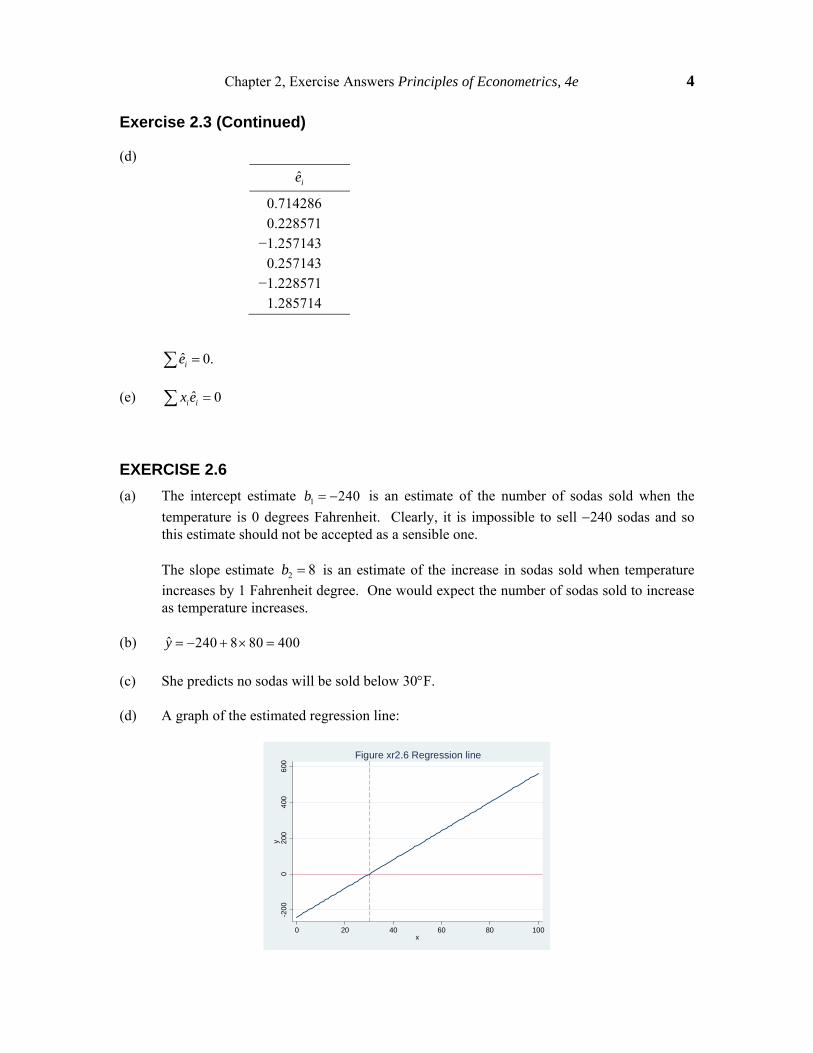
(d)
ie
0.714286 0.228571
−1.257143 0.257143
−1.228571 1.285714
ˆ 0.ie
(e) ˆ 0i ix e
EXERCISE 2.6
(a) The intercept estimate 1 240b is an estimate of the number of sodas sold when the
temperature is 0 degrees Fahrenheit. Clearly, it is impossible to sell 240 sodas and so this estimate should not be accepted as a sensible one.
The slope estimate 2 8b is an estimate of the increase in sodas sold when temperature
increases by 1 Fahrenheit degree. One would expect the number of sodas sold to increase as temperature increases.
(b) ˆ 240 8 80 400y
(c) She predicts no sodas will be sold below 30F. (d) A graph of the estimated regression line:
-200
02
004
006
00y
0 20 40 60 80 100x
Figure xr2.6 Regression line

Chapter 2, Exercise Answers Principles of Econometrics, 4e 5
EXERCISE 2.9
(a)
The repair period comprises those months between the two vertical lines. The graphical
evidence suggests that the damaged motel had the higher occupancy rate before and after the repair period. During the repair period, the damaged motel and the competitors had similar occupancy rates.
(b) A plot of MOTEL_PCT against COMP_PCT yields:
There appears to be a positive relationship the two variables. Such a relationship may exist as both the damaged motel and the competitor(s) face the same demand for motel rooms.
30
40
50
60
70
80
90
100
0 2 4 6 8 10 12 14 16 18 20 22 24 26
month, 1=march 2003,.., 25=march 2005
percentage motel occupancypercentage competitors occupancy
Figure xr2.9a Occupancy Rates
40
50
60
70
80
90
100
40 50 60 70 80
percentage competitors occupancy
pe
rcen
tage
mot
el o
ccu
pan
cy
Figure xr2.9b Observations on occupancy
Chapter 2, Exercise Answers Principles of Econometrics, 4e 6
Exercise 2.9 (continued)
(c) _ 21.40 0.8646 _MOTEL PCT COMP PCT .
The competitors’ occupancy rates are positively related to motel occupancy rates, as expected. The regression indicates that for a one percentage point increase in competitor occupancy rate, the damaged motel’s occupancy rate is expected to increase by 0.8646 percentage points.
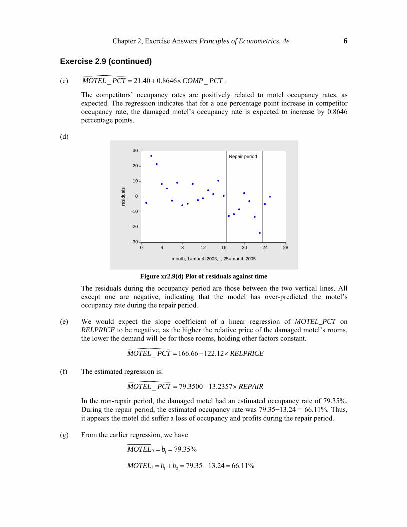
(d)
Figure xr2.9(d) Plot of residuals against time
The residuals during the occupancy period are those between the two vertical lines. All except one are negative, indicating that the model has over-predicted the motel’s occupancy rate during the repair period.
(e) We would expect the slope coefficient of a linear regression of MOTEL_PCT on RELPRICE to be negative, as the higher the relative price of the damaged motel’s rooms, the lower the demand will be for those rooms, holding other factors constant.
_ 166.66 122.12MOTEL PCT RELPRICE
(f) The estimated regression is:
_ 79.3500 13.2357MOTEL PCT REPAIR
In the non-repair period, the damaged motel had an estimated occupancy rate of 79.35%. During the repair period, the estimated occupancy rate was 79.35−13.24 = 66.11%. Thus, it appears the motel did suffer a loss of occupancy and profits during the repair period.
(g) From the earlier regression, we have
0 1 79.35%MOTEL b
1 1 2 79.35 13.24 66.11%MOTEL b b
-30
-20
-10
0
10
20
30
0 4 8 12 16 20 24 28
month, 1=march 2003,.., 25=march 2005
resi
du
als
Repair period

Chapter 2, Exercise Answers Principles of Econometrics, 4e 7
Exercise 2.9(g) (continued)
For competitors, the estimated regression is:
_ 62.4889 0.8825COMP PCT REPAIR
0 1
1 1 2
62.49%
62.49 0.88 63.37%
COMP b
COMP b b
During the non-repair period, the difference between the average occupancies was:
0 0 79.35 62.49 16.86%MOTEL COMP
During the repair period it was
1 1 66.11 63.37 2.74%MOTEL COMP
This comparison supports the motel’s claim for lost profits during the repair period. When there were no repairs, their occupancy rate was 16.86% higher than that of their competitors; during the repairs it was only 2.74% higher.
(h) _ _ 16.8611 14.1183MOTEL PCT COMP PCT REPAIR
The intercept estimate in this equation (16.86) is equal to the difference in average
occupancies during the non-repair period, 0 0MOTEL COMP . The sum of the two
coefficient estimates 16.86 ( 14.12) 2.74 is equal to the difference in average
occupancies during the repair period, 1 1MOTEL COMP .
This relationship exists because averaging the difference between two series is the same as taking the difference between the averages of the two series.
EXERCISE 2.12
(a) and (b) 30069 9181.7SPRICE LIVAREA
The coefficient 9181.7 suggests that selling price increases by approximately $9182 for each additional 100 square foot in living area. The intercept, if taken literally, suggests a house with zero square feet would cost $30,069, a meaningless value.
0
200000
400000
600000
800000
10 20 30 40 50living area, hundreds of square feet
selling price of home, dollars Fitted values
Figure xr2.12b Observations and fitted line

Chapter 2, Exercise Answers Principles of Econometrics, 4e 8
Exercise 2.12 (continued)
(c) The estimated quadratic equation for all houses in the sample is
257728 212.611SPRICE LIVAREA
The marginal effect of an additional 100 square feet for a home with 1500 square feet of living space is:
slope 2 212.611 2 212.611 15 6378.33 d SPRICE
LIVAREA =dLIVAREA
That is, adding 100 square feet of living space to a house of 1500 square feet is estimated to increase its expected price by approximately $6378.
(d)
The quadratic model appears to fit the data better; it is better at capturing the
proportionally higher prices for large houses.
SSE of linear model, (b): 2 12ˆ 2.23 10iSSE e
SSE of quadratic model, (c): 2 12ˆ 2.03 10iSSE e
The SSE of the quadratic model is smaller, indicating that it is a better fit.
(e) Large lots: 2113279 193.83SPRICE LIVAREA
Small lots: 262172 186.86SPRICE LIVAREA
The intercept can be interpreted as the expected price of the land – the selling price for a house with no living area. The coefficient of LIVAREA has to be interpreted in the context of the marginal effect of an extra 100 square feet of living area, which is 22 LIVAREA .
Thus, we estimate that the mean price of large lots is $113,279 and the mean price of small lots is $62,172. The marginal effect of living area on price is $387.66 LIVAREA for houses on large lots and $373.72 LIVAREA for houses on small lots.
0
200000
400000
600000
800000
10 20 30 40 50living area, hundreds of square feet
selling price of home, dollars Fitted valuesFitted values
Figure xr2.12d Linear and quadratic fitted lines

Chapter 2, Exercise Answers Principles of Econometrics, 4e 9
Exercise 2.12 (continued)
(f) The following figure contains the scatter diagram of PRICE and AGE as well as the
estimated equation 137404 627.16SPRICE AGE . We estimate that the expected selling price is $627 less for each additional year of age. The estimated intercept, if taken literally, suggests a house with zero age (i.e., a new house) would cost $137,404.
The following figure contains the scatter diagram of ln(PRICE) and AGE as well as the
estimated equation ln 11.746 0.00476SPRICE AGE . In this estimated model, each
extra year of age reduces the selling price by 0.48%. To find an interpretation from the intercept, we set 0AGE , and find an estimate of the price of a new home as
exp ln exp(11.74597) $126,244SPRICE
Based on the plots and visual fit of the estimated regression lines, the log-linear model shows much less of problem with under-prediction and so it is preferred.
(g) The estimated equation for all houses is 115220 133797SPRICE LGELOT . The estimated expected selling price for a house on a large lot (LGELOT = 1) is 115220+133797 = $249017. The estimated expected selling price for a house not on a large lot (LGELOT = 0) is $115220.
0
200000
400000
600000
800000
0 20 40 60 80 100age of home at time of sale, years
selling price of home, dollars Fitted values
Figure xr2.12f sprice vs age regression line
10
11
12
13
14
0 20 40 60 80 100age of home at time of sale, years
lsprice Fitted values
Figure xr2.12f log(sprice) vs age regression line

Chapter 2, Exercise Answers Principles of Econometrics, 4e 10
EXERCISE 2.14
(a) and (b)
There appears to be a positive association between VOTE and GROWTH.
The estimated equation for 1916 to 2008 is
50.848 0.88595VOTE GROWTH
The coefficient 0.88595 suggests that for a 1 percentage point increase in the growth rate of GDP in the 3 quarters before the election there is an estimated increase in the share of votes of the incumbent party of 0.88595 percentage points.
We estimate, based on the fitted regression intercept, that that the incumbent party’s expected vote is 50.848% when the growth rate in GDP is zero. This suggests that when there is no real GDP growth, the incumbent party will still maintain the majority vote.
(c) The estimated equation for 1916 - 2004 is
51.053 0.877982VOTE GROWTH
The actual 2008 value for growth is 0.220. Putting this into the estimated equation, we obtain the predicted vote share for the incumbent party:
2008 200851.053 0.877982 51.053 0.877982 0.220 51.246VOTE GROWTH
This suggests that the incumbent party will maintain the majority vote in 2008. However, the actual vote share for the incumbent party for 2008 was 46.60, which is a long way short of the prediction; the incumbent party did not maintain the majority vote.
30
40
50
60
Incu
mbe
nt v
ote
-15 -10 -5 0 5 10Growth rate before election
Incumbent share of the two-party presidential vote Fitted values
xr2-14 Vote versus Growth with fitted regression

Chapter 2, Exercise Answers Principles of Econometrics, 4e 11
Exercise 2.14 (continued)
(d)
There appears to be a negative association between the two variables.
The estimated equation is:
53.408 0.444312VOTE = INFLATION
We estimate that a 1 percentage point increase in inflation during the incumbent party’s first 15 quarters reduces the share of incumbent party’s vote by 0.444 percentage points.
The estimated intercept suggests that when inflation is at 0% for that party’s first 15 quarters, the expected share of votes won by the incumbent party is 53.4%; the incumbent party is predicted to maintain the majority vote when inflation, during its first 15 quarters, is at 0%.
30
40
50
60
Incu
mbe
nt v
ote
0 2 4 6 8Inflation rate before election
Incumbent share of the two-party presidential vote Fitted values
xr2-14 Vote versus Inflation

12
CHAPTER 3
Exercise Answers
EXERCISE 3.3
(a) Reject 0H because 3.78 2.819.ct t
(b) Reject 0H because 3.78 2.508.ct t
(c) Do not reject 0H because 3.78 1.717.ct t
Figure xr3.3 One tail rejection region
(d) Reject 0H because 2.32 2.074.ct t
(e) A 99% interval estimate of the slope is given by (0.079, 0.541)

Chapter 3, Exercise Answers, Principles of Econometrics, 4e 13
EXERCISE 3.6
(a) We reject the null hypothesis because the test statistic value t = 4.265 > tc = 2.500. The p-value is 0.000145
Figure xr3.6(a) Rejection region and p-value
(b) We do not reject the null hypothesis because the test statistic value
2.093 2.500ct t . The p-value is 0.0238
Figure xr3.6(b) Rejection region and p-value
(c) Since 2.221 1.714ct t , we reject 0H at a 5% significance level.
(d) A 95% interval estimate for 2 is given by ( 25.57, 0.91) .
(e) Since 3.542 2.500ct t , we reject 0H at a 5% significance level.
(f) A 95% interval estimate for 2 is given by ( 22.36, 5.87) .

Chapter 3, Exercise Answers, Principles of Econometrics, 4e 14
EXERCISE 3.9
(a) We set up the hypotheses H0: 2 0 versus H1: 2 0 . Since t = 4.870 > 1.717, we
reject the null hypothesis.
(b) A 95% interval estimate for 2 from the regression in part (a) is (0.509, 1.263).
(c) We set up the hypotheses H0: 2 0 versus H1: 2 0 . Since 0.741 1.717t , we
do not reject the null hypothesis.
(d) A 95% interval estimate for 2 from the regression in part (c) is ( 1.688, 0.800).
(e) We test 0 1: 50H against the alternative 1 1: 50H . Since 1.515 1.717t , we do
not reject the null hypothesis.
(f) The 95% interval estimate is 49.40, 55.64 .
EXERCISE 3.13
(a)
Figure xr3.13(a) Scatter plot of ln(WAGE) against EXPER30
(b) The estimated log-polynomial model is 2ln 2.9826 0.0007088WAGE EXPER30 .
We test 0 2: 0H against the alternative 1 2: 0H . Because 8.067 1.646t , we
reject 0 2: 0H .
0.5
1.0
1.5
2.0
2.5
3.0
3.5
4.0
4.5
-30 -20 -10 0 10 20 30 40
EXPER30
LNW
AG
E

Chapter 3, Exercise Answers, Principles of Econometrics, 4e 15
Exercise 3.13 (continued)
(c)
10
10
me 0.4215
EXPER
d WAGE
d EXPER
30
30
me 0.0
EXPER
d WAGE
d EXPER
50
50
me 0.4215
EXPER
d WAGE
d EXPER
(d)
Figure xr3.13(d) Plot of fitted and actual values of WAGE
0
10
20
30
40
50
60
70
80
-30 -20 -10 0 10 20 30 40
EXPER30
WAGEfitted WAGE

16
CHAPTER 4
Exercise Answers
EXERCISE 4.1
(a) 2 0.71051R
(b) 2 0.8455R
(c) 2ˆ 6.4104
EXERCISE 4.2
(a) ˆ 5.83 17.38
(1.23) (2.34)
y x where
20
xx
(b) ˆ 0.1166 0.01738
(0.0246) (0.00234)
y x
ˆˆwhere
50
yy
(c) ˆ 0.2915 0.869
(0.0615) (0.117)
y x
ˆˆwhere and
20 20
y xy x
EXERCISE 4.9
(a) Equation 1: 0ˆ 0.69538 0.015025 48 1.417y
0 (0.975,45)ˆ ( ) 1.4166 2.0141 0.25293 (0.907,1.926)y t se f
Equation 2: 0ˆ 0.56231 0.16961 ln(48) 1.219y
0 (0.975,45)ˆ ( ) 1.2189 2.0141 0.28787 (0.639,1.799)y t se f
Equation 3: 20ˆ 0.79945 0.000337543 (48) 1.577y
0 (0.975,45)ˆ ( ) 1.577145 2.0141 0.234544 (1.105, 2.050)y t se f
The actual yield in Chapman was 1.844.

Chapter 4, Exercise Answers, Principles of Econometrics, 4e 17
Exercise 4.9 (continued)
(b) Equation 1:
0.0150tdy
dt
Equation 2:
0.0035tdy
dt
Equation 3:
0.0324tdy
dt
(c) Equation 1:
0.509t
t
dy t
dt y
Equation 2:
0.139t
t
dy t
dt y
Equation 3:
0.986t
t
dy t
dt y
(d) The slopes dy dt and the elasticities dy dt t y give the marginal change in yield
and the percentage change in yield, respectively, that can be expected from technological change in the next year. The results show that the predicted effect of technological change is very sensitive to the choice of functional form.
EXERCISE 4.11
(a) The estimated regression model for the years 1916 to 2008 is:
250.8484 0.8859 0.5189
(se) 1.0125 0.1819
VOTE GROWTH R
2008 51.043VOTE
20082008 4.443VOTE VOTE
(b) The estimated regression model for the years 1916 to 2004 is:
251.0533 0.8780 0.5243
(se) (1.0379) (0.1825)
VOTE GROWTH R
2008 51.246VOTE
20082008 4.646f VOTE VOTE
This prediction error is larger in magnitude than the least squares residual. This result is expected because the estimated regression in part (b) does not contain information about VOTE in the year 2008.

Chapter 4, Exercise Answers, Principles of Econometrics, 4e 18
Exercise 4.11 (continued)
(c) 2008 (0.975,21) se( ) 51.2464 2.0796 4.9185 (41.018,61.475)VOTE t f
The actual 2008 outcome 2008 46.6VOTE falls within this prediction interval.
(d) 1.086GROWTH
EXERCISE 4.13
(a) The regression results are:
ln( ) 10.5938 0.000596
se 0.0219 0.000013
484.84 46.30
PRICE SQFT
t
The coefficient 0.000596 suggests an increase of one square foot is associated with a 0.06% increase in the price of the house.
67.23dPRICE
dSQFT
2elasticity = 0.00059596 1611.9682 0.9607SQFT
(b) The regression results are:
ln( ) 4.1707 1.0066ln( )
se 0.1655 0.0225
25.20 44.65
PRICE SQFT
t
The coefficient 1.0066 says that an increase in living area of 1% is associated with a 1% increase in house price.
The coefficient 1.0066 is the elasticity.
70.444dPRICE
dSQFT
(c) From the linear function, 2 0.672R .
From the log-linear function in part (a), 2 0.715gR .
From the log-log function in part (b), 2 0.673gR .

Chapter 4, Exercise Answers, Principles of Econometrics, 4e 19
Exercise 4.13 (continued)
(d) Jarque-Bera = 78.85
p -value = 0.0000
Jarque-Bera = 52.74
p -value = 0.0000
Jarque-Bera = 2456
p -value = 0.0000
Figure xr4.13(d) Histogram of residuals for
log-linear model
Figure xr4.13(d) Histogram of residuals for
log-log model
Figure xr4.13(d) Histogram of residuals for
simple linear model
All Jarque-Bera values are significantly different from 0 at the 1% level of significance. We can conclude that the residuals are not compatible with an assumption of normality, particularly in the simple linear model.
0
20
40
60
80
100
120
-0.75 -0.50 -0.25 0.00 0.25 0.50 0.75
0
20
40
60
80
100
120
-0.75 -0.50 -0.25 0.00 0.25 0.50 0.75
0
40
80
120
160
200
-100000 0 100000 200000

Chapter 4, Exercise Answers, Principles of Econometrics, 4e 20
Exercise 4.13 (continued)
(e)
Residuals of log-linear model Residuals of log-log model
Residuals of simple linear model
The residuals appear to increase in magnitude as SQFT increases. This is most evident in
the residuals of the simple linear functional form. Furthermore, the residuals for the simple linear model in the area less than 1000 square feet are all positive indicating that perhaps the functional form does not fit well in this region.
(f) Prediction for log-linear model: 203,516PRICE
Prediction for log-log model: 188,221PRICE
Prediction for simple linear model: 201,365PRICE
(g) The standard error of forecast for the log-linear model is se( ) 0.20363f .
The 95% confidence interval is: (133,683; 297,316) .
The standard error of forecast for the log-log model is se( ) 0.20876f .
The 95% confidence interval is (122,267; 277,454) .
The standard error of forecast for the simple linear model is se( ) 30348.26f .
The 95% confidence interval is 141,801; 260,928 .
-0.8
-0.4
0.0
0.4
0.8
1.2
0 1000 2000 3000 4000 5000
SQFT
resi
du
al
-0.8
-0.4
0.0
0.4
0.8
1.2
0 1000 2000 3000 4000 5000
SQFT
resi
du
al
-150000
-100000
-50000
0
50000
100000
150000
200000
250000
0 1000 2000 3000 4000 5000
SQFT
resi
da
ul
Chapter 4, Exercise Answers, Principles of Econometrics, 4e 21
Exercise 4.13 (continued)
(h) The simple linear model is not a good choice because the residuals are heavily skewed to the right and hence far from being normally distributed. It is difficult to choose between the other two models – the log-linear and log-log models. Their residuals have similar patterns and they both lead to a plausible elasticity of price with respect to changes in square feet, namely, a 1% change in square feet leads to a 1% change in price. The log-linear model is favored on the basis of its higher 2
gR value, and its smaller standard
deviation of the error, characteristics that suggest it is the model that best fits the data.

22
CHAPTER 5
Exercise Answers
EXERCISE 5.1
(a) 2 31, 0, 0y x x
*2ix *
3ix *iy
0 1 0 1 2 1 2 1 2
2 0 2 1 1 1
2 1 2 0 1 1
1 1 0 1 0 1
(b) 2 2* * * ** *2 2 3 313, 16, 4, 10i i i i i iy x x y x x
(c) 2 0.8125b 3 0.4b 1 1b
(d) ˆ 0.4, 0.9875, 0.025, 0.375, 1.4125, 0.025, 0.6, 0.4125, 0.1875e
(e) 2ˆ 0.6396
(f) 23 0r
(g) 2se( ) 0.1999b
(h) 3.8375 16SSE SST 212.1625 0.7602SSR R

Chapter 5, Exercise Answers, Principles of Econometrics, 4e 23
EXERCISE 5.2
(a) 2 (0.975,6) 2se( ) (0.3233, 1.3017)b t b
(b) We do not reject 0H because 0.9377t and 0.9377 2.447 = (0.975, 6)t .
EXERCISE 5.4
(a) The regression results are:
20.0315 0.0414ln 0.0001 0.0130 0.0247
se (0.0322) (0.0071) (0.0004) (0.0055)
WTRANS TOTEXP AGE NK R
(b) The value 2 0.0414b suggests that as ln TOTEXP increases by 1 unit the budget
proportion for transport increases by 0.0414. Alternatively, one can say that a 10% increase in total expenditure will increase the budget proportion for transportation by 0.004. (See Chapter 4.3.3.) The positive sign of 2b is according to our expectation because
as households become richer they tend to use more luxurious forms of transport and the proportion of the budget for transport increases.
The value 3 0.0001b implies that as the age of the head of the household increases by 1
year the budget share for transport decreases by 0.0001. The expected sign for 3b is not
clear. For a given level of total expenditure and a given number of children, it is difficult to predict the effect of age on transport share.
The value 4 0.0130b implies that an additional child decreases the budget share for
transport by 0.013. The negative sign means that adding children to a household increases expenditure on other items (such as food and clothing) more than it does on transportation. Alternatively, having more children may lead a household to turn to cheaper forms of transport.
(c) The p-value for testing 0 3: 0H against the alternative 1 3: 0H where 3 is the
coefficient of AGE is 0.869, suggesting that AGE could be excluded from the equation. Similar tests for the coefficients of the other two variables yield p-values less than 0.05.
(d) 2 0.0247R
(e) For a one-child household: 0 0.1420WTRANS
For a two-child household: 0 0.1290WTRANS
Chapter 5, Exercise Answers, Principles of Econometrics, 4e 24
EXERCISE 5.8
(a) Equations describing the marginal effects of nitrogen and phosphorus on yield are
8.011 3.888 0.567E YIELD
NITRO PHOSNITRO
4.800 1.556 0.567E YIELD
PHOS NITROPHOS
The marginal effect of both fertilizers declines – we have diminishing marginal products – and these marginal effects eventually become negative. Also, the marginal effect of one fertilizer is smaller, the larger is the amount of the other fertilizer that is applied.
(b) (i) The marginal effects when 1NITRO and 1PHOS are
3.556E YIELD
NITRO
2.677E YIELD
PHOS
(ii) The marginal effects when 2NITRO and 2PHOS are
0.899E YIELD
NITRO
0.554E YIELD
PHOS
When 1NITRO and 1PHOS , the marginal products of both fertilizers are positive. Increasing the fertilizer applications to 2NITRO and 2PHOS reduces the marginal effects of both fertilizers, with that for nitrogen becoming negative.
(c) To test these hypotheses, the coefficients are defined according to the following equation
2 21 2 3 4 5 6YIELD NITRO PHOS NITRO PHOS NITRO PHOS e
(i) Testing 0 2 4 6: 2 0H against the alternative 1 2 4 6: 2 0H , the t-value
is 7.367t . Since t > (0.975, 21) 2.080ct t , we reject the null hypothesis and
conclude that the marginal effect of nitrogen on yield is not zero when NITRO = 1 and PHOS = 1.
(ii) Testing 0 2 4 6: 4 0H against 1 2 4 6: 4 0H , the t-value is 1.660t .
Since |t| < 2.080 (0.975, 21)t , we do not reject the null hypothesis. A zero marginal yield
with respect to nitrogen cannot be rejected when NITRO = 1 and PHOS = 2.
(iii) Testing 0 2 4 6: 6 0H against 1 2 4 6: 6 0H , the t-value is 8.742t .
Since |t| > 2.080 (0.975, 21)t , we reject the null hypothesis and conclude that the
marginal product of yield to nitrogen is not zero when NITRO = 3 and PHOS = 1.
(d) The maximizing levels are 1.701NITRO and 2.465PHOS . The yield maximizing levels of fertilizer are not necessarily the optimal levels. The optimal levels are those where the marginal cost of the inputs is equal to their marginal value product.

Chapter 5, Exercise Answers, Principles of Econometrics, 4e 25
EXERCISE 5.15
(a) The estimated regression model is:
52.16 0.6434 0.1721
(se) (1.46) (0.1656) (0.4290)
VOTE GROWTH INFLATION
The hypothesis test results on the significance of the coefficients are:
0 2 1 2: 0 : 0H H p-value = 0.0003 significant at 10% level
0 3 1 3: 0 : 0H H p-value = 0.3456 not significant at 10% level
One-tail tests were used because more growth is considered favorable, and more inflation is considered not favorable, for re-election of the incumbent party.
(b) (i) For 4INFLATION and 3GROWTH , 0 49.54VOTE .
(ii) For 4INFLATION and 0GROWTH , 0 51.47VOTE .
(iii) For 4INFLATION and 3GROWTH , 0 53.40VOTE .
(c) (i) When 4INFLATION and 3GROWTH , the hypotheses are
0 1 2 3 1 1 2 3: 3 4 50 : 3 4 50H H
The calculated t-value is 0.399t . Since (0.99,30)0.399 2.457 t , we do not
reject 0H . There is no evidence to suggest that the incumbent part will get the
majority of the vote when 4INFLATION and 3GROWTH .
(ii) When 4INFLATION and 0GROWTH , the hypotheses are
0 1 3 1 1 3: 4 50 : 4 50H H
The calculated t-value is 1.408t . Since (0.99,30)1.408 2.457 t , we do not reject
0H . There is insufficient evidence to suggest that the incumbent part will get the
majority of the vote when 4INFLATION and 0GROWTH .
(iii) When 4INFLATION and 3GROWTH , the hypotheses are
0 1 2 3 1 1 2 3: 3 4 50 : 3 4 50H H
The calculated t-value is 2.950t . Since (0.99,30)2.950 2.457 t , we reject 0H . We
conclude that the incumbent part will get the majority of the vote when 4INFLATION and 3GROWTH .
As a president seeking re-election, you would not want to conclude that you would be re-elected without strong evidence to support such a conclusion. Setting up re-election as the alternative hypothesis with a 1% significance level reflects this scenario.

Chapter 5, Exercise Answers, Principles of Econometrics, 4e 26
EXERCISE 5.23
The estimated model is
2 339.594 47.024 20.222 2.749
(se) (28.153) (27.810) (8.901) (0.925)
SCORE AGE AGE AGE
The within sample predictions, with age expressed in terms of years (not units of 10 years) are graphed in the following figure. They are also given in a table on page 27.
Figure xr5.23 Fitted line and observations (a) We test 0 4: 0.H The t-value is 2.972, with corresponding p-value 0.0035. We
therefore reject 0H and conclude that the quadratic function is not adequate. For suitable
values of 2 3 4, and , the cubic function can decrease at an increasing rate, then go past
a point of inflection after which it decreases at a decreasing rate, and then it can reach a minimum and increase. These are characteristics worth considering for a golfer. That is, the golfer improves at an increasing rate, then at a decreasing rate, and then declines in ability. These characteristics are displayed in Figure xr5.23.
(b) (i) Age = 30
(ii) Between the ages of 20 and 25.
(iii) Between the ages of 25 and 30.
(iv) Age = 36.
(v) Age = 40.
(c) No. At the age of 70, the predicted score (relative to par) for Lion Forrest is 241.71. To break 100 it would need to be less than 28 ( 100 72) .
-15
-10
-5
0
5
10
15
20 24 28 32 36 40 44
AGE_UNITS
SCORESCOREHAT

Chapter 5, Exercise Answers, Principles of Econometrics, 4e 27
Exercise 5.23 (continued)
Predicted scores at different ages
age predicted scores
20 4.4403 21 4.5621 22 4.7420 23 4.9633 24 5.2097 25 5.4646 26 5.7116 27 5.9341 28 6.1157 29 6.2398 30 6.2900 31 6.2497 32 6.1025 33 5.8319 34 5.4213 35 4.8544 36 4.1145 37 3.1852 38 2.0500 39 0.6923 40 0.9042 41 2.7561 42 4.8799 43 7.2921 44 10.0092

Chapter 5, Exercise Answers, Principles of Econometrics, 4e 28
EXERCISE 5.24
(a) The coefficient estimates, standard errors, t-values and p-values are in the following table.
Dependent Variable: ln(PROD)
Coeff Std. Error t-value p-value
C -1.5468 0.2557 -6.0503 0.0000
ln(AREA) 0.3617 0.0640 5.6550 0.0000
ln(LABOR) 0.4328 0.0669 6.4718 0.0000
ln(FERT) 0.2095 0.0383 5.4750 0.0000
All estimates have elasticity interpretations. For example, a 1% increase in labor will lead
to a 0.4328% increase in rice output. A 1% increase in fertilizer will lead to a 0.2095% increase in rice output. All p-values are less than 0.0001 implying all estimates are significantly different from zero at conventional significance levels.
(b) Testing 0 2: 0.5H against 1 2: 0.5H , the t-value is 2.16t .
Since (0.995,348)2.59 2.16 2.59 t , we do not reject 0H . The data are compatible with
the hypothesis that the elasticity of production with respect to land is 0.5.
(c) A 95% interval estimate of the elasticity of production with respect to fertilizer is given by
4 (0.975,348) 4se( ) (0.134, 0.285)b t b
This relatively narrow interval implies the fertilizer elasticity has been precisely measured.
(d) Testing 0 3: 0.3H against 1 3: 0.3H , the t-value is 1.99t . We reject 0H because
(0.95,348)1.99 1.649 t . There is evidence to conclude that the elasticity of production with
respect to labor is greater than 0.3. Reversing the hypotheses and testing 0 3: 0.3H
against 1 3: 0.3H , leads to a rejection region of 1.649t . The calculated t-value is
1.99t . The null hypothesis is not rejected because 1.99 1.649 .

29
CHAPTER 6
Exercise Answers
EXERCISE 6.3
(a) Let the total variation, unexplained variation and explained variation be denoted by SST, SSE and SSR, respectively. Then, we have
42.8281SSE 802.0243SST 759.1962SSR
(b) A 95% confidence interval for 2 is
2 (0.975,17) 2se( ) (0.2343,1.1639)b t b
A 95% confidence interval for 3 is
2 (0.975,17) 3se( ) (1.3704, 2.1834)b t b
(c) To test H0: 2 1 against the alternative H1: 2 < 1, we calculate 1.3658t . Since
(0.05,17)1.3658 1.740 t , we fail to reject 0H . There is insufficient evidence to
conclude 2 1 .
(d) To test 0 2 3: 0H against the alternative 1 2: 0H and/or 3 0 , we calculate
151F . Since (0.95,2,17)151 3.59 F , we reject H0 and conclude that the hypothesis 2 =
3 = 0 is not compatible with the data.
(e) The t-value for testing 0 2 3: 2H against the alternative 1 2 3: 2H is
2 3
2 3
2 0.378620.634
se 2 0.59675
b bt
b b
Since (0.025,17)2.11 0.634 2.11 t , we do not reject 0H . There is no evidence to
suggest that 2 32 .

Chapter 6, Exercise Answers, Principles of Econometrics, 4e 30
EXERCISE 6.5
(a) The null and alternative hypotheses are:
0 2 4 3 5
1 2 4 3 5
: and
: or or both
H
H
(b) The restricted model assuming the null hypothesis is true is
2 2
1 4 5 6ln( ) ( ) ( )WAGE EDUC EXPER EDUC EXPER HRSWK e
(c) The F-value is 70.32F .The critical value at a 5% significance level is
(0.95,2,994) 3.005F . Since the F-value is greater than the critical value, we reject the null
hypothesis and conclude that education and experience have different effects on ln( )WAGE .
EXERCISE 6.10
(a) The restricted and unrestricted least squares estimates and their standard errors appear in the following table. The two sets of estimates are similar except for the noticeable difference in sign for ln(PL). The positive restricted estimate 0.187 is more in line with our a priori views about the cross-price elasticity with respect to liquor than the negative estimate 0.583. Most standard errors for the restricted estimates are less than their counterparts for the unrestricted estimates, supporting the theoretical result that restricted least squares estimates have lower variances.
CONST ln(PB) ln(PL) ln(PR) ln( )I
Unrestricted 3.243 1.020 0.583 0.210 0.923 (3.743) (0.239) (0.560) (0.080) (0.416)
Restricted 4.798 1.299 0.187 0.167 0.946 (3.714) (0.166) (0.284) (0.077) (0.427)
(b) The high auxiliary 2sR and sample correlations between the explanatory variables that appear in the following table suggest that collinearity could be a problem. The relatively large standard error and the wrong sign for ln( )PL are a likely consequence of this
correlation.
Sample Correlation With
Variable Auxiliary R2 ln(PL) ln(PR) ln(I)
ln(PB) 0.955 0.967 0.774 0.971 ln(PL) 0.955 0.809 0.971 ln(PR) 0.694 0.821 ln(I) 0.964

Chapter 6, Exercise Answers, Principles of Econometrics, 4e 31
Exercise 6.10 (continued)
(c) Testing 0 2 3 4 5: 0H against 1 2 3 4 5: 0H , the value of the test
statistic is F = 2.50, with a p-value of 0.127. The critical value is (0.95,1,25) 4.24F . We do
not reject 0H . The evidence from the data is consistent with the notion that if prices and
income go up in the same proportion, demand will not change.
(d)(e) The results for parts (d) and (e) appear in the following table.
ln(Q) Q
ln( )Q se( )f tc lower upper lower upper
(d) Restricted 4.5541 0.14446 2.056 4.257 4.851 70.6 127.9
(e) Unrestricted 4.4239 0.16285 2.060 4.088 4.759 59.6 116.7
EXERCISE 6.12
The RESET results for the log-log and the linear demand function are reported in the table below.
Test F-value df 5% Critical F p-value
Log-log 1 term 0.0075 (1,24) 4.260 0.9319 2 terms 0.3581 (2,23) 3.422 0.7028
Linear 1 term 8.8377 (1,24) 4.260 0.0066 2 terms 4.7618 (2,23) 3.422 0.0186
Because the RESET returns p-values less than 0.05 (0.0066 and 0.0186 for one and two
terms respectively), at a 5% level of significance, we conclude that the linear model is not an adequate functional form for the beer data. On the other hand, the log-log model appears to suit the data well with relatively high p-values of 0.9319 and 0.7028 for one and two terms respectively. Thus, based on the RESET we conclude that the log-log model better reflects the demand for beer.
EXERCISE 6.20
(a) Testing 0 2 3:H against 1 2 3:H , the calculated F-value is 0.342. We do not
reject 0H because (0.95,1,348)0.342 3.868 F . The p-value of the test is 0.559. The
hypothesis that the land and labor elasticities are equal cannot be rejected at a 5% significance level.
Using a t-test, we fail to reject 0H because 0.585t and the critical values are
(0.025,348) 1.967t and (0.975,348) 1.967t . The p-value of the test is 0.559.

Chapter 6, Exercise Answers, Principles of Econometrics, 4e 32
Exercise 6.20 (continued)
(b) Testing 0 2 3 4: 1H against 1 2 3 4: 1H , the F-value is 0.0295. The t-
value is 0.172t . The critical values are (0.90,1,348) 2.72F or (0.95,348) 1.649t and
(0.05,348) 1.649t . The p-value of the test is 0.864. The hypothesis of constant returns to
scale cannot be rejected at a 10% significance level.
(c) The null and alternative hypotheses are
2 30
2 3 4
0:
1H
2 31
2 3 4
0 and/or:
1H
The critical value is (0.95,2,348) 3.02F . The calculated F-value is 0.183. The p-value of the
test is 0.833. The joint null hypothesis of constant returns to scale and equality of land and labor elasticities cannot be rejected at a 5% significance level.
(d) The estimates and (standard errors) from the restricted models, and the unrestricted model, are given in the following table. Because the unrestricted estimates almost satisfy the restriction 2 3 4 1 , imposing this restriction changes the unrestricted estimates
and their standard errors very little. Imposing the restriction 2 3 has an impact,
changing the estimates for both 2 and 3 , and reducing their standard errors
considerably. Adding 2 3 4 1 to this restriction reduces the standard errors even
further, leaving the coefficient estimates essentially unchanged.
Unrestricted 2 3 2 3 4 1 2 3
2 3 4 1
C –1.5468 –1.4095 –1.5381 –1.4030 (0.2557) (0.1011) (0.2502) (0.0913)
ln( )AREA 0.3617 0.3964 0.3595 0.3941 (0.0640) (0.0241) (0.0625) (0.0188)
ln( )LABOR 0.4328 0.3964 0.4299 0.3941 (0.0669) (0.0241) (0.0646) (0.0188)
ln( )FERT 0.2095 0.2109 0.2106 0.2118 (0.0383) (0.0382) (0.0377) (0.0376)
SSE 40.5654 40.6052 40.5688 40.6079

Chapter 6, Exercise Answers, Principles of Econometrics, 4e 33
EXERCISE 6.21
Full FERT LABOR AREA model omitted omitted omitted
2 ( )b AREA 0.3617 0.4567 0.6633
3 ( )b LABOR 0.4328 0.5689 0.7084
4 ( )b FERT 0.2095 0.3015 0.2682
RESET(1) p-value 0.5688 0.8771 0.4281 0.1140 RESET(2) p-value 0.2761 0.4598 0.5721 0.0083
(i) With FERT omitted the elasticity for AREA changes from 0.3617 to 0.4567, and the
elasticity for LABOR changes from 0.4328 to 0.5689. The RESET F-values (p-values) for 1 and 2 extra terms are 0.024 (0.877) and 0.779 (0.460), respectively. Omitting FERT appears to bias the other elasticities upwards, but the omitted variable is not picked up by the RESET.
(ii) With LABOR omitted the elasticity for AREA changes from 0.3617 to 0.6633, and the elasticity for FERT changes from 0.2095 to 0.3015. The RESET F-values (p-values) for 1 and 2 extra terms are 0.629 (0.428) and 0.559 (0.572), respectively. Omitting LABOR also appears to bias the other elasticities upwards, but again the omitted variable is not picked up by the RESET.
(iii) With AREA omitted the elasticity for FERT changes from 0.2095 to 0.2682, and the elasticity for LABOR changes from 0.4328 to 0.7084. The RESET F-values (p-values) for 1 and 2 extra terms are 2.511 (0.114) and 4.863 (0.008), respectively. Omitting AREA appears to bias the other elasticities upwards, particularly that for LABOR. In this case the omitted variable misspecification has been picked up by the RESET with two extra terms.
EXERCISE 6.22
(a) 7.40F Fc = 3.26 p-value = 0.002
We reject H0 and conclude that age does affect pizza expenditure.
(b) Point estimates, standard errors and 95% interval estimates for the marginal propensity to spend on pizza for different ages are given in the following table.
Age Point Standard Confidence Interval
Estimate Error Lower Upper
20 4.515 1.520 1.432 7.598 30 3.283 0.905 1.448 4.731 40 2.050 0.465 1.107 2.993
50 0.818 0.710 0.622 2.258
55 0.202 0.991 1.808 2.212
Chapter 6, Exercise Answers, Principles of Econometrics, 4e 34
Exercise 6.22 (continued)
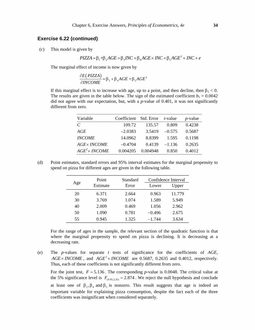
(c) This model is given by
21 2 3 4 5+PIZZA AGE INC AGE INC AGE INC e
The marginal effect of income is now given by
2
3 4 5+E PIZZA
AGE AGEINCOME
If this marginal effect is to increase with age, up to a point, and then decline, then 5 < 0. The results are given in the table below. The sign of the estimated coefficient b5 = 0.0042 did not agree with our expectation, but, with a p-value of 0.401, it was not significantly different from zero.
Variable Coefficient Std. Error t-value p-value
C 109.72 135.57 0.809 0.4238
AGE –2.0383 3.5419 –0.575 0.5687
INCOME 14.0962 8.8399 1.595 0.1198
AGE INCOME –0.4704 0.4139 –1.136 0.2635
AGE2 INCOME 0.004205 0.004948 0.850 0.4012
(d) Point estimates, standard errors and 95% interval estimates for the marginal propensity to spend on pizza for different ages are given in the following table.
Age Point Standard Confidence Interval
Estimate Error Lower Upper
20 6.371 2.664 0.963 11.779 30 3.769 1.074 1.589 5.949 40 2.009 0.469 1.056 2.962
50 1.090 0.781 0.496 2.675
55 0.945 1.325 1.744 3.634
For the range of ages in the sample, the relevant section of the quadratic function is that
where the marginal propensity to spend on pizza is declining. It is decreasing at a decreasing rate.
(e) The p-values for separate t tests of significance for the coefficients of AGE, AGE INCOME , and 2AGE INCOME are 0.5687, 0.2635 and 0.4012, respectively. Thus, each of these coefficients is not significantly different from zero.
For the joint test, 5.136F . The corresponding p-value is 0.0048. The critical value at the 5% significance level is (0.95,3,35) 2.874F . We reject the null hypothesis and conclude
at least one of 2 4 5, and is nonzero. This result suggests that age is indeed an
important variable for explaining pizza consumption, despite the fact each of the three coefficients was insignificant when considered separately.

Chapter 6, Exercise Answers, Principles of Econometrics, 4e 35
Exercise 6.22 (continued)
(f) Two ways to check for collinearity are (i) to examine the simple correlations between each pair of variables in the regression, and (ii) to examine the R2 values from auxiliary regressions where each explanatory variable is regressed on all other explanatory variables in the equation. In the tables below there are 3 simple correlations greater than 0.94 for the regression in part (c) and 5 when 3AGE INC is included. The number of auxiliary regressions with R2s greater than 0.99 is 3 for the regression in part (c) and 4 when
3AGE INC is included. Thus, collinearity is potentially a problem. Examining the estimates and their standard errors confirms this fact. In both cases there are no t-values which are greater than 2 and hence no coefficients are significantly different from zero. None of the coefficients are reliably estimated. In general, including squared and cubed variables can lead to collinearity if there is inadequate variation in a variable.
Simple Correlations
AGE AGE INC 2AGE INC 3AGE INC
INC 0.4685 0.9812 0.9436 0.8975 AGE 0.5862 0.6504 0.6887 AGE INC 0.9893 0.9636
2AGE INC 0.9921
R2 Values from Auxiliary Regressions
LHS variable R2 in part (c) R2 in part (f)
INC 0.99796 0.99983 AGE 0.68400 0.82598 AGE INC 0.99956 0.99999
2AGE INC 0.99859 0.99999 3AGE INC 0.99994

36
CHAPTER 7
Exercise Answers
EXERCISE 7.2
(a) Intercept: At the beginning of the time period over which observations were taken, on a day which is not Friday, Saturday or a holiday, and a day which has neither a full moon nor a half moon, the estimated average number of emergency room cases was 93.69.
T: We estimate that the average number of emergency room cases has been increasing by 0.0338 per day, other factors held constant. The t-value is 3.06 and p-value = 0.003 < 0.01.
HOLIDAY: The average number of emergency room cases is estimated to go up by 13.86 on holidays, holding all else constant. The “holiday effect” is significant at the 0.05 level.
FRI and SAT: The average number of emergency room cases is estimated to go up by 6.9 and 10.6 on Fridays and Saturdays, respectively, holding all else constant. These estimated coefficients are both significant at the 0.01 level.
FULLMOON: The average number of emergency room cases is estimated to go up by 2.45 on days when there is a full moon, all else constant. However, a null hypothesis stating that a full moon has no influence on the number of emergency room cases would not be rejected at any reasonable level of significance.
NEWMOON: The average number of emergency room cases is estimated to go up by 6.4 on days when there is a new moon, all else held constant. However, a null hypothesis stating that a new moon has no influence on the number of emergency room cases would not be rejected at the usual 10% level, or smaller.
(b) There are very small changes in the remaining coefficients, and their standard errors, when FULLMOON and NEWMOON are omitted.
(c) Testing 0 6 7: 0H against 1 6 7: or is nonzeroH , we find 1.29F . The 0.05
critical value is (0.95, 2, 222) 3.307F , and corresponding p-value is 0.277. Thus, we do not
reject the null hypothesis that new and full moons have no impact on the number of emergency room cases.

Chapter 7, Exercise Answers, Principles of Econometrics, 4e 37
EXERCISE 7.5
(a) The estimated equation, with standard errors in parentheses, is
ln 4.4638 0.3334 0.03596 0.003428
(se) 0.0264 0.0359 0.00104 0.001414
PRICE UTOWN SQFT SQFT UTOWN
20.000904 0.01899 0.006556 0.8619
0.000218 0.00510 0.004140
AGE POOL FPLACE R
(b) Using this result for the coefficients of SQFT and AGE, we estimate that an additional 100
square feet of floor space is estimated to increase price by 3.6% for a house not in University town and 3.25% for a house in University town, holding all else fixed. A house which is a year older is estimated to sell for 0.0904% less, holding all else constant. The estimated coefficients of UTOWN, AGE, and the slope-indicator variable SQFT_UTOWN are significantly different from zero at the 5% level of significance.
(c) An approximation of the percentage change in price due to the presence of a pool is 1.90%. The exact percentage change in price due to the presence of a pool is estimated to be 1.92%.
(d) An approximation of the percentage change in price due to the presence of a fireplace is 0.66%. The exact percentage change in price due to the presence of a fireplace is also 0.66%.
(e) The percentage change in price attributable to being near the university, for a 2500 square-feet home, is 28.11%.
EXERCISE 7.9
(a) The estimated average test scores are:
regular sized class with no aide = 918.0429 regular sized class with aide = 918.3568 small class = 931.9419
From the above figures, the average scores are higher with the small class than the regular class. The effect of having a teacher aide is negligible.
The results of the estimated models for parts (b)-(g) are summarized in the table on page 38. (b) The coefficient of SMALL is the difference between the average of the scores in the
regular sized classes (918.36) and the average of the scores in small classes (931.94). That is b2 = 931.9419 − 918.0429 = 13.899. Similarly the coefficient of AIDE is the difference between the average score in classes with an aide and regular classes. The t-value for the significance of 3 is 0.136t . The critical value at the 5% significance level is 1.96. We
cannot conclude that there is a significant difference between test scores in a regular class and a class with an aide.

Chapter 7, Exercise Answers, Principles of Econometrics, 4e 38
Exercise 7.9 (continued)
Exercise 7-9
--------------------------------------------------------------------------------------------
(1) (2) (3) (4) (5)
(b) (c) (d) (e) (g)
--------------------------------------------------------------------------------------------
C 918.043*** 904.721*** 923.250*** 931.755*** 918.272***
(1.641) (2.228) (3.121) (3.940) (4.357)
SMALL 13.899*** 14.006*** 13.896*** 13.980*** 15.746***
(2.409) (2.395) (2.294) (2.302) (2.096)
AIDE 0.314 -0.601 0.698 1.002 1.782
(2.310) (2.306) (2.209) (2.217) (2.025)
TCHEXPER 1.469*** 1.114*** 1.156*** 0.720***
(0.167) (0.161) (0.166) (0.167)
BOY -14.045*** -14.008*** -12.121***
(1.846) (1.843) (1.662)
FREELUNCH -34.117*** -32.532*** -34.481***
(2.064) (2.126) (2.011)
WHITE_ASIAN 11.837*** 16.233*** 25.315***
(2.211) (2.780) (3.510)
TCHWHITE -7.668*** -1.538
(2.842) (3.284)
TCHMASTERS -3.560* -2.621
(2.019) (2.184)
SCHURBAN -5.750** .
(2.858) .
SCHRURAL -7.006*** .
(2.559) .
--------------------------------------------------------------------------------------------
N 5786 5766 5766 5766 5766
adj. R-sq 0.007 0.020 0.101 0.104 0.280
BIC 66169.500 65884.807 65407.272 65418.626 64062.970
SSE 31232400.314 30777099.287 28203498.965 28089837.947 22271314.955
--------------------------------------------------------------------------------------------
Standard errors in parentheses
* p<0.10, ** p<0.05, *** p<0.01
(c) The t-statistic for the significance of the coefficient of TCHEXPER is 8.78 and we reject the null hypothesis that a teacher’s experience has no effect on total test scores. The inclusion of this variable has a small impact on the coefficient of SMALL, and the coefficient of AIDE has gone from positive to negative. However AIDE’s coefficient is not significantly different from zero and this change is of negligible magnitude, so the sign change is not important.
(d) The inclusion of BOY, FREELUNCH and WHITE_ASIAN has little impact on the coefficients of SMALL and AIDE. The variables themselves are statistically significant at the 0.01 level of significance.

Chapter 7, Exercise Answers, Principles of Econometrics, 4e 39
Exercise 7.9 (continued)
(e) The regression result suggests that TCHWHITE, SCHRURAL and SCHURBAN are significant at the 5% level and TCHMASTERS is significant at the 10% level. The inclusion of these variables has only a very small and negligible effect on the estimated coefficients of AIDE and SMALL.
(f) The results found in parts (c), (d) and (e) suggest that while some additional variables were found to have a significant impact on total scores, the estimated advantage of being in small classes, and the insignificance of the presence of a teacher aide, is unaffected. The fact that the estimates of the key coefficients did not change is support for the randomization of student assignments to the different class sizes. The addition or deletion of uncorrelated factors does not affect the estimated effect of the key variables.
(g) We find that inclusion of the school effects increases the estimates of the benefits of small classes and the presence of a teacher aide, although the latter effect is still insignificant statistically. The F-test of the joint significance of the school indicators is 19.15. The 5% F-critical value for 78 numerator and 5679 denominator degrees of freedom is 1.28, thus we reject the null hypothesis that all the school effects are zero, and conclude that at least some are not zero.
The variables SCHURBAN and SCHRURAL drop out of this model because they are exactly collinear with the included 78 indicator variables.
EXERCISE 7.14
(a) We expect the parameter estimate for the dummy variable PERSON to be positive because of reputation and knowledge of the incumbent. However, it could be negative if the incumbent was, on average, unpopular and/or ineffective. We expect the parameter estimate for WAR to be positive reflecting national feeling during and immediately after first and second world wars.
(b) The regression functions for each value of PARTY are:
1 7 2 3 4
5 6 8
| 1E VOTE PARTY GROWTH INFLATION GOODNEWS
PERSON DURATION WAR
1 7 2 3 4
5 6 8
| 1E VOTE PARTY GROWTH INFLATION GOODNEWS
PERSON DURATION WAR
The intercept when there is a Democrat incumbent is 1 7 . When there is a Republican
incumbent it is 1 7 . Thus, the effect of PARTY on the vote is 72 with the sign of 7
indicating whether incumbency favors Democrats 7( 0) or Republicans 7( 0) .

Chapter 7, Exercise Answers, Principles of Econometrics, 4e 40
Exercise 7.14 (continued)
(c) The estimated regression using observations for 1916-2004 is
47.2628 0.6797 0.6572 1.0749
(se) 2.5384 0.1107 0.2914 0.2493
3.2983 3.3300 2.6763 5.6149
1.4081 1.2124 0.6264 2.6879
VOTE GROWTH INFLATION GOODNEWS
PERSON DURATION PARTY WAR
The signs are as expected. Can you explain why? All the estimates are statistically significant at a 1% level of significance except for INFLATION, PERSON, DURATION and WAR. The coefficients of INFLATION, DURATION and PERSON are statistically significant at a 5% level, however. The coefficient of WAR is statistically insignificant at a level of 5%. Lastly, an R2 of 0.9052 suggests that the model fits the data very well.
(d) Using the data for 2008, and based on the estimates from part (c), we summarize the actual and predicted vote as follows, along with a listing of the values of the explanatory variables.
vote growth inflation goodnews person duration party war votehat
46.6 .22 2.88 3 0 1 -1 0 48.09079
Thus, we predict that the Republicans, as the incumbent party, will lose the 2008 election with 48.091% of the vote. This prediction was correct, with Democrat Barack Obama defeating Republican John McCain with 52.9% of the popular vote to 45.7%.
(e) A 95% confidence interval for the vote in the 2008 election is
2012 (0.975,15) se( ) (42.09, 54.09)VOTE t f
(f) For the 2012 election the Democratic party will have been in power for one term and so we set DURATION = 1 and PARTY = 1. Also, the incumbent, Barack Obama, is running for election and so we set PERSON = 1. WAR = 0. We use the value of inflation 3.0% anticipating higher rates of inflation after the policy stimulus. We consider 3 scenarios for GROWTH and GOODNEWS representing good economic outcomes, moderate and poor, if there is a “double-dip” recession. The values and the prediction intervals based on regression estimates with data from 1916-2008, are
GROWTH INFLATION GOODNEWS lb vote ub 3.5 3 6 45.6 51.5 57.3 1 3 3 40.4 46.5 52.5 -3 3 1 35.0 41.5 48.0
We see that if there is good economic performance, then President Obama can expect to be re-elected. If there is poor economic performance, then we predict he will lose the election with the upper bound of the 95% prediction interval for a vote in his favor being only 48%. In the intermediate case, with only modest growth and less good news, then we predict he will lose the election, though the interval estimate upper bound is greater than 50%, meaning that anything could happen.

Chapter 7, Exercise Answers, Principles of Econometrics, 4e 41
EXERCISE 7.16
(a) The histogram for PRICE is positively skewed. On the other hand, the logarithm of PRICE is much less skewed and is more symmetrical. Thus, the histogram of the logarithm of PRICE is closer in shape to a normal distribution than the histogram of PRICE.
Figure xr7.16(a) Histogram of PRICE
Figure xr7.16(b) Histogram of ln(PRICE)
01
02
03
0P
erc
ent
0 200000 400000 600000 800000selling price of home, dollars
05
10
15
Pe
rcen
t
10 11 12 13 14log(selling price)
Chapter 7, Exercise Answers, Principles of Econometrics, 4e 42
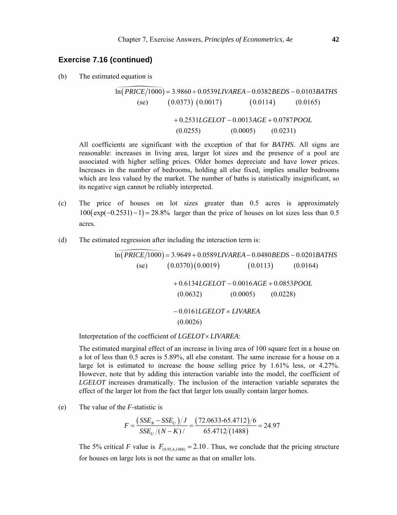
Exercise 7.16 (continued)
(b) The estimated equation is
ln 1000 3.9860 0.0539 0.0382 0.0103
(se) 0.0373 0.0017 0.0114 (0.0165)
0.2531 0.0013 0.0787
(0.
PRICE LIVAREA BEDS BATHS
LGELOT AGE POOL
0255) (0.0005) (0.0231)
All coefficients are significant with the exception of that for BATHS. All signs are reasonable: increases in living area, larger lot sizes and the presence of a pool are associated with higher selling prices. Older homes depreciate and have lower prices. Increases in the number of bedrooms, holding all else fixed, implies smaller bedrooms which are less valued by the market. The number of baths is statistically insignificant, so its negative sign cannot be reliably interpreted.
(c) The price of houses on lot sizes greater than 0.5 acres is approximately
100 exp( 0.2531) 1 28.8% larger than the price of houses on lot sizes less than 0.5
acres.
(d) The estimated regression after including the interaction term is:
ln 1000 3.9649 0.0589 0.0480 0.0201
(se) 0.0370 0.0019 0.0113 (0.0164)
0.6134 0.0016 0.0853
(0.
PRICE LIVAREA BEDS BATHS
LGELOT AGE POOL
0632) (0.0005) (0.0228)
0.0161
(0.0026)
LGELOT LIVAREA
Interpretation of the coefficient of LGELOTLIVAREA:
The estimated marginal effect of an increase in living area of 100 square feet in a house on a lot of less than 0.5 acres is 5.89%, all else constant. The same increase for a house on a large lot is estimated to increase the house selling price by 1.61% less, or 4.27%. However, note that by adding this interaction variable into the model, the coefficient of LGELOT increases dramatically. The inclusion of the interaction variable separates the effect of the larger lot from the fact that larger lots usually contain larger homes.
(e) The value of the F-statistic is
72.0633-65.4712 6
24.97( ) / 65.4712 1488
R U
U
SSE SSE JF
SSE N K
The 5% critical F value is (0.95,6,1488) 2.10F . Thus, we conclude that the pricing structure
for houses on large lots is not the same as that on smaller lots.

Chapter 7, Exercise Answers, Principles of Econometrics, 4e 43
Exercise 7.16 (continued)
A summary of the alternative model estimations follows.
Exercise 7-16
----------------------------------------------------------------------------
(1) (2) (3) (4)
LGELOT=1 LGELOT=0 Rest Unrest
----------------------------------------------------------------------------
C 4.4121*** 3.9828*** 3.9794*** 3.9828***
(0.183) (0.037) (0.039) (0.038)
LIVAREA 0.0337*** 0.0604*** 0.0607*** 0.0604***
(0.005) (0.002) (0.002) (0.002)
BEDS -0.0088 -0.0522*** -0.0594*** -0.0522***
(0.048) (0.012) (0.012) (0.012)
BATHS 0.0827 -0.0334** -0.0262 -0.0334*
(0.066) (0.017) (0.017) (0.017)
AGE -0.0018 -0.0016*** -0.0008* -0.0016***
(0.002) (0.000) (0.000) (0.000)
POOL 0.1259* 0.0697*** 0.0989*** 0.0697***
(0.074) (0.024) (0.024) (0.025)
LGELOT 0.4293***
(0.141)
LOT_AREA -0.0266***
(0.004)
LOT_BEDS 0.0434
(0.037)
LOT_BATHS 0.1161**
(0.052)
LOT_AGE -0.0002
(0.001)
LOT_POOL 0.0562
(0.060)
----------------------------------------------------------------------------
N 95 1405 1500 1500
adj. R-sq 0.676 0.608 0.667 0.696
BIC 50.8699 -439.2028 -252.8181 -352.8402
SSE 7.1268 58.3445 72.0633 65.4712
----------------------------------------------------------------------------
Standard errors in parentheses
* p<0.10, ** p<0.05, *** p<0.01
** LOT_X indicates interaction between LGELOT and X

44
CHAPTER 8
Exercise Answers
EXERCISE 8.7
(a) 20 31.1 89.35 52.34i i i i ix y x y x
0 3.8875x y
2 2 22
8 89.35 0 31.1=1.7071
8 52.34 0i i i i
i i
N x y x yb
N x x
1 2 3.8875 1.7071 0 3.8875b y b x
(b)
observation e 2ˆln( )e 2ˆln( )z e
1 1.933946 1.319125 4.353113 2 0.733822 0.618977 0.185693 3 9.549756 4.513031 31.591219 4 1.714707 1.078484 5.068875 5 3.291665 2.382787 4.527295 6 3.887376 2.715469 18.465187 7 3.484558 2.496682 5.742369 8 3.746079 2.641419 16.905082
(c) We use the estimating equation
2ˆln( )i i ie z v
Using least squares to estimate from this model is equivalent to a simple linear regression without a constant term. The least squares estimate for is
Chapter 8, Exercise Answers, Principles of Econometrics, 4e 45
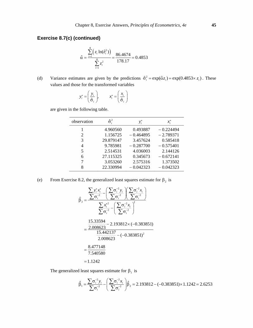
Exercise 8.7(c) (continued)
82
18
2
1
ˆln( )86.4674
ˆ 0.4853178.17
i ii
ii
z e
z
(d) Variance estimates are given by the predictions 2 ˆˆ exp( ) exp(0.4853 )i i iz z . These
values and those for the transformed variables
* *,ˆ ˆ
i ii i
i i
y xy x
are given in the following table.
observation 2ˆ i *iy *
ix
1 4.960560 0.493887 0.224494 2 1.156725 0.464895 2.789371 3 29.879147 3.457624 0.585418 4 9.785981 0.287700 0.575401 5 2.514531 4.036003 2.144126 6 27.115325 0.345673 0.672141 7 3.053260 2.575316 1.373502 8 22.330994 0.042323 0.042323
(e) From Exercise 8.2, the generalized least squares estimate for 2 is
2 2
2 2 2
2 22 2
2 2
2
ˆ
15.335942.193812 ( 0.383851)
2.00862315.442137
( 0.383851)2.008623
8.477148
7.540580
1.1242
i i i i i i
i i i
i i i
i i
y x y x
x x
The generalized least squares estimate for 1 is
2 2
1 22 2ˆ ˆ 2.193812 ( 0.383851) 1.1242 2.6253i i i i
i i
y x

Chapter 8, Exercise Answers, Principles of Econometrics, 4e 46
EXERCISE 8.10
(a) The transformed model corresponding to the variance assumption 2 2i ix is
1 2
1where i i
i i i
i i i
y ex e e
x x x
Squaring the residuals and regressing them on ix gives
2 2ˆ 123.79 23.35 0.13977e x R
2 2 40 0.13977 5.59N R
A null hypothesis of no heteroskedasticity is rejected. The variance assumption 2 2i ix
was not adequate to eliminate heteroskedasticity. (b) The transformed model used to obtain the estimates in (8.27) is
1 2
1where
ˆ ˆ ˆ ˆi i i
i ii i i i
y x ee e
ˆ exp(0.93779596 2.32923872 ln( )i ix
Squaring the residuals and regressing them on ix gives
2 2ˆ 1.117 0.05896 0.02724e x R
2 2 40 0.02724 1.09N R
A null hypothesis of no heteroskedasticity is not rejected. The variance assumption 2 2i ix is adequate to eliminate heteroskedasticity.
EXERCISE 8.13
(a) For the model 2 31 1 2 1 3 1 4 1 1t t t t tC Q Q Q e , where 2
1 1var t te Q , the generalized
least squares estimates of 1, 2, 3 and 4 are:
estimated coefficient
standard error
1 93.595 23.422 2 68.592 17.484
3 10.744 3.774 4 1.0086 0.2425
(b) The calculated F value for testing the hypothesis that 1 = 4 = 0 is 108.4. The 5% critical
value from the F(2,24) distribution is 3.40. Since the calculated F is greater than the critical F, we reject the null hypothesis that 1 = 4 = 0.
Chapter 8, Exercise Answers, Principles of Econometrics, 4e 47
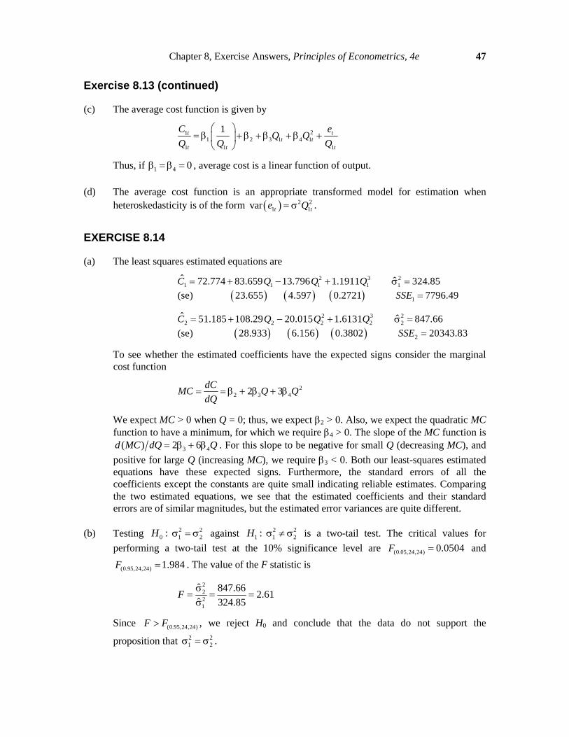
Exercise 8.13 (continued)
(c) The average cost function is given by
211 2 3 1 4 1
1 1 1
1t tt t
t t t
C eQ Q
Q Q Q
Thus, if 1 4 0 , average cost is a linear function of output.
(d) The average cost function is an appropriate transformed model for estimation when
heteroskedasticity is of the form 2 21 1var t te Q .
EXERCISE 8.14
(a) The least squares estimated equations are
2 3 21 1 1 1 1
1
ˆ ˆ72.774 83.659 13.796 1.1911 324.85
(se) 23.655 4.597 0.2721 7796.49
C Q Q Q
SSE
2 3 22 2 2 2 2
2
ˆ ˆ51.185 108.29 20.015 1.6131 847.66
(se) 28.933 6.156 0.3802 20343.83
C Q Q Q
SSE
To see whether the estimated coefficients have the expected signs consider the marginal cost function
22 3 42 3
dCMC Q Q
dQ
We expect MC > 0 when Q = 0; thus, we expect 2 > 0. Also, we expect the quadratic MC function to have a minimum, for which we require 4 > 0. The slope of the MC function is
3 4( ) 2 6d MC dQ Q . For this slope to be negative for small Q (decreasing MC), and
positive for large Q (increasing MC), we require 3 < 0. Both our least-squares estimated equations have these expected signs. Furthermore, the standard errors of all the coefficients except the constants are quite small indicating reliable estimates. Comparing the two estimated equations, we see that the estimated coefficients and their standard errors are of similar magnitudes, but the estimated error variances are quite different.
(b) Testing 2 20 1 2:H against 2 2
1 1 2:H is a two-tail test. The critical values for
performing a two-tail test at the 10% significance level are (0.05,24,24) 0.0504F and
(0.95,24,24) 1.984F . The value of the F statistic is
2221
ˆ 847.662.61
ˆ 324.85F
Since (0.95,24,24)F F , we reject H0 and conclude that the data do not support the
proposition that 2 21 2 .

Chapter 8, Exercise Answers, Principles of Econometrics, 4e 48
Exercise 8.14 (continued)
(c) Since the test outcome in (b) suggests 2 21 2 , but we are assuming both firms have the
same coefficients, we apply generalized least squares to the combined set of data, with the observations transformed using 1 and 2 . The estimated equation is
2 3ˆ 67.270 89.920 15.408 1.3026
(se) 16.973 3.415 0.2065
C Q Q Q
Remark: Some automatic software commands will produce slightly different results if the transformed error variance is restricted to be unity or if the variables are transformed using variance estimates from a pooled regression instead of those from part (a).
(d) Although we have established that 2 21 2 , it is instructive to first carry out the test for
0 1 1 2 2 3 3 4 4: , , ,H
under the assumption that 2 21 2 , and then under the assumption that 2 2
1 2 .
Assuming that 2 21 2 , the test is equivalent to the Chow test discussed on pages 268-270
of the text. The test statistic is
R U
U
SSE SSE JF
SSE N K
where USSE is the sum of squared errors from the full dummy variable model. The
dummy variable model does not have to be estimated, however. We can also calculate
USSE as the sum of the SSE from separate least squares estimation of each equation. In
this case 1 2 7796.49 20343.83 28140.32USSE SSE SSE
The restricted model has not yet been estimated under the assumption that 2 21 2 . Doing
so by combining all 56 observations yields 28874.34RSSE . The F-value is given by
(28874.34 28140.32) 4
0.31328140.32 (56 8)
R U
U
SSE SSE JF
SSE N K
The corresponding 2 -value is 2 4 1.252F . These values are both much less than
their respective 5% critical values (0.95,4,48) 2.565F and 2(0.95,4) 9.488 . There is no
evidence to suggest that the firms have different coefficients. In the formula for F, note that the number of observations N is the total number from both firms, and K is the number of coefficients from both firms.
The above test is not valid in the presence of heteroskedasticity. It could give misleading results. To perform the test under the assumption that 2 2
1 2 , we follow the same steps,
but we use values for SSE computed from transformed residuals. For restricted estimation from part (c) the result is 49.2412RSSE . For unrestricted estimation, we have the
interesting result

Chapter 8, Exercise Answers, Principles of Econometrics, 4e 49
Exercise 8.14(d) (continued)
2 2
* 1 2 1 1 1 2 2 21 1 2 22 2 2 2
1 2 1 2
ˆ ˆ( ) ( )48
ˆ ˆ ˆ ˆU
SSE SSE N K N KSSE N K N K
Thus,
(49.2412 48) 4
0.310348 48
F
and 2 1.241
The same conclusion is reached. There is no evidence to suggest that the firms have different coefficients.
The 2 and F test values can also be conveniently calculated by performing a Wald test on
the coefficients after running weighted least squares on a pooled model that includes dummy variables to accommodate the different coefficients.
EXERCISE 8.15
(a) To estimate the two variances using the variance model specified, we first estimate the equation
1 2 3 4i i i i iWAGE EDUC EXPER METRO e
From this equation we use the squared residuals to estimate the equation
21 2ˆln( )i i ie METRO v
The estimated parameters from this regression are 1ˆ 1.508448 and 2ˆ 0.338041 .
Using these estimates, we have
METRO = 0 2ˆ exp(1.508448 0.338041 0) 4.519711R
METRO = 1, 2ˆ exp(1.508448 0.338041 1) 6.337529M
These error variance estimates are much smaller than those obtained from separate sub-samples ( 2ˆ 31.824M and 2ˆ 15.243R ). One reason is the bias factor from the
exponential function – see page 317 of the text. Multiplying 2ˆ 6.3375M and 2ˆ 4.5197R by the bias factor exp(1.2704) yields 2ˆ 22.576M and 2ˆ 16.100R . These
values are closer, but still different from those obtained using separate sub-samples. The differences occur because the residuals from the combined model are different from those from the separate sub-samples.
(b) To use generalized least squares, we use the estimated variances above to transform the
model in the same way as in (8.35). After doing so the regression results are, with standard errors in parentheses
9.7052 1.2185 0.1328 1.5301
(se) 1.0485 0.0694 0.0150 0.3858i i i iWAGE EDUC EDUC METRO

Chapter 8, Exercise Answers, Principles of Econometrics, 4e 50
Exercise 8.15(b) (continued)
The magnitudes of these estimates and their standard errors are almost identical to those in equation (8.36). Thus, although the variance estimates can be sensitive to the estimation technique, the resulting generalized least squares estimates of the mean function are much less sensitive.
(c) The regression output using White standard errors is
9.9140 1.2340 0.1332 1.5241
(se) 1.2124 0.0835 0.0158 0.3445i i i iWAGE EDUC EDUC METRO
With the exception of that for METRO, these standard errors are larger than those in part (b), reflecting the lower precision of least squares estimation.

51
CHAPTER 9
Exercise Answers
EXERCISE 9.4
(a) Using hand calculations
1
21
2
1
ˆ ˆ0.0979
0.06341.5436ˆ
T
t tt
T
tt
e er
e
,
23
22
1
ˆ ˆ0.1008
0.06531.5436ˆ
T
t tt
T
tt
e er
e
(b) (i) For testing 0 1: 0H against 1 1: 0H , 1 10 0.0634 0.201Z T r . Critical
values are (0.025) 1.96Z and (0.975) 1.96Z . We do not reject the null hypothesis
and conclude that 1r is not significantly different from zero.
(ii) For testing 0 2: 0H against 1 2: 0H , 2 10 0.0653 0.207Z T r . Critical
values are (0.025) 1.96Z and (0.975) 1.96Z . We do not reject the null hypothesis
and conclude that 2r is not significantly different from zero.
The significance bounds are drawn at 1.96 10 0.62 . With this small sample,
the autocorrelations are a long way from being significantly different from zero.
-.6
-.4
-.2
.0
.2
.4
.6
1 2
Chapter 9, Exercise Answers, Principles of Econometrics, 4e 52
EXERCISE 9.7
(a) Under the assumptions of the AR(1) model, corr( , ) kt t ke e . Thus,
(i) 1corr( , ) 0.9t te e
(ii) 4 44corr( , ) 0.9 0.6561t te e
(iii) 2
22 2
15.263
1 1 0.9v
e
(b) (i) 1corr( , ) 0.4t te e
(ii) 4 44corr( , ) 0.4 0.0256t te e
(iii) 2
22 2
11.190
1 1 0.4v
e
When the correlation between the current and previous period error is weaker, the correlations between the current error and the errors at more distant lags die out relatively quickly, as is illustrated by a comparison of 4 0.6561 in part (a)(ii) with 4 0.0256
in part (b)(ii). Also, the larger the correlation , the greater the variance 2e , as is
illustrated by a comparison of 2 5.263e in part (a)(iii) with 2 1.190e in part (b)(iii).
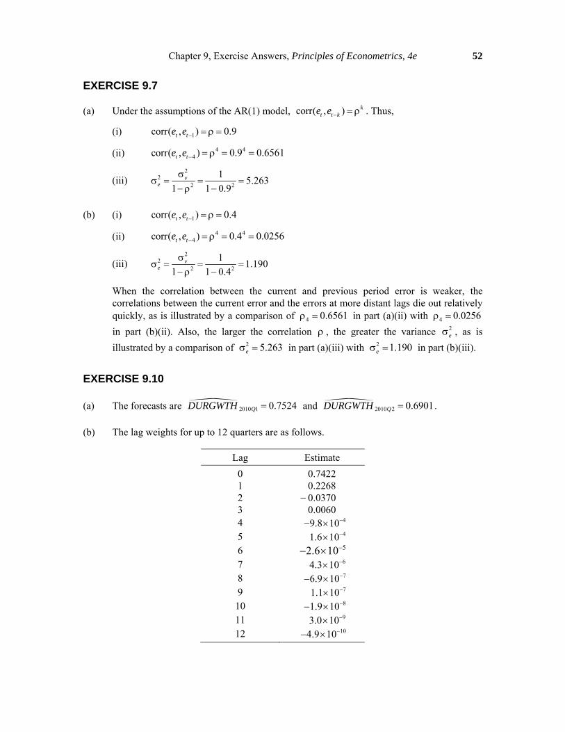
EXERCISE 9.10
(a) The forecasts are 2010 1 0.7524QDURGWTH and 2010 2 0.6901QDURGWTH .
(b) The lag weights for up to 12 quarters are as follows.
Lag Estimate
0 0.7422 1 0.2268 2 0.0370 3 0.0060 4 49.8 10 5 41.6 10 6 52.6 10 7 64.3 10 8 76.9 10 9 71.1 10
10 81.9 10 11 93.0 10 12 104.9 10

Chapter 9, Exercise Answers, Principles of Econometrics, 4e 53
Exercise 9.10 (continued)
(c) The one and two-quarter delay multipliers are
1
1
β 0.2268t
t
DURGWTH
INGRWTH
22
β 0.0370t
t
DURGWTH
INGRWTH
These values suggest that if income growth increases by 1% and then returns to its original level in the next quarter, then growth in the consumption of durables will increase by 0.227% in the next quarter and decrease by 0.037% two quarters later.
The one and two-quarter interim multipliers are
0 1
0 1 2
ˆ ˆβ β 0.7422 0.2268 0.969
ˆ ˆ ˆβ β β 0.969 0.0370 0.932
These values suggest that if income growth increases by 1% and is maintained at its new level, then growth in the consumption of durables will increase by 0.969% in the next quarter and increase by 0.932% two quarters later.
The total multiplier is 0β 0.9373jj
. This value suggests that if income growth
increases by 1% and is maintained at its new level, then, at the new equilibrium, growth in the consumption of durables will increase by 0.937%.
EXERCISE 9.12
(a) Coefficient Estimates and AIC and SC Values for Finite Distributed Lag Model
0q 1q 2q 3q 4q 5q 6q
0.4229 0.5472 0.5843 0.5828 0.6002 0.5990 0.5239
0 0.3119 0.2135 0.1974 0.1972 0.1940 0.1940 0.1830
1 0.1954 0.1693 0.1699 0.1726 0.1728 0.1768
2 0.0707 0.0713 0.0664 0.0662 0.0828
3 0.0021 0.0065 0.0062 0.0192
4 0.0222 0.0225 0.0475
5 0.0015 0.0169
6 0.0944
AIC 3.1132 3.4314 3.4587 3.4370 3.4188 3.3971 3.4416AIC* 0.2753 0.5935 0.6208 0.5991 0.5809 0.5592 0.6037SC 3.0584 3.3492 3.3490 3.2999 3.2543 3.2052 3.2223SC* 0.2205 0.5113 0.5111 0.4620 0.4165 0.3673 0.3844
Note: AIC* = AIC 1 ln(2 ) and SC* = SC 1 ln(2 )
The AIC is minimized at 2q while the SC is minimized at 1q .

Chapter 9, Exercise Answers, Principles of Econometrics, 4e 54
Exercise 9.12 (continued)
(b) (i) A 95% confidence interval for 0 is given by
0 00.975,88ˆ ˆse 0.1974 1.987 0.0328 ( 0.2626, 0.1322)t
(ii) The null and alternative hypotheses are
0 0 1 2 1 0 1 2: β β β 0.5 : β β β 0.5H H
The test statistic is
0 1 2
0 1 2
( 0.5) 0.0626561.815
se 0.034526
b b bt
b b b
The critical value is 0.95,88 1.662t . Since 1.815 1.662t , we reject the null
hypothesis and conclude that the total multiplier is greater than 0.5. The p-value is 0.0365.
(iii) The estimated normal growth rate is ˆ 0.58427 0.437344 1.336NG . The 95%
confidence interval for the normal growth rate is
0.975,88ˆ ˆse 1.336 1.987 0.0417 (1.253,1.419)N NG t G
EXERCISE 9.15
ln( ) 3.8933 0.7761ln( )
(0.0613) (0.2771) least squares se's
(0.0624) (0.3782) HAC se's
AREA PRICE
(a) The correlogram for the residuals is
The significant bounds used are 1.96 34 0.336 . Autocorrelations 1 and 5 are
significantly different from zero.
-.4
-.3
-.2
-.1
.0
.1
.2
.3
.4
.5
2 4 6 8 10 12 14 16 18 20 22 24

Chapter 9, Exercise Answers, Principles of Econometrics, 4e 55
Exercise 9.15 (continued)
(b) The null and alternative hypotheses are 0: ρ 0H and 0: ρ 0H , and the test statistic is
5.4743LM , yielding a p-value of 0.0193. Since the p-value is less than 0.05, we reject the null hypothesis and conclude that there is evidence of autocorrelation at the 5 percent significance level.
(c) The 95% confidence intervals are:
(i) Using least square standard errors
2 20.975,32 se( ) 0.7761 2.0369 0.2775 (0.2109,1.3413)b t b
(ii) Using HAC standard errors
2 20.975,32 se( ) 0.7761 2.0369 0.3782 (0.0057,1.5465)b t b
The wider interval under HAC standard errors shows that ignoring serially correlated errors gives an exaggerated impression about the precision of the least-squares estimated elasticity of supply.
(d) The estimated equation under the assumption of AR(1) errors is
1ln( ) 3.8988 0.8884ln( ) 0.4221
(se) (0.0922) (0.2593) (0.1660)t t t t tAREA PRICE e e v
The t-value for testing whether the estimate for ρ is significantly different from zero is
0.4221 0.1660 2.542t , with a p-value of 0.0164. We conclude that is significantly
different from zero at a 5% level. A 95% confidence interval for the elasticity of supply is
2 20.975,30 se( ) 0.8884 2.0423 0.2593 (0.3588,1.4179)b t b
This confidence interval is narrower than the one from HAC standard errors in part (c), reflecting the increased precision from recognizing the AR(1) error. It is also slightly narrower than the one from least squares, although we cannot infer much from this difference because the least squares standard errors are incorrect.
(e) We write the ARDL(1,1) model as
1 1 0 1 1ln( ) δ θ ln( ) δ ln( ) δ ln( ) t t t t tAREA AREA PRICE PRICE e
The estimated model is
1 1ln( ) 2.3662 0.4043ln( ) 0.7766ln( ) 0.6109ln( )
(0.6557) (0.1666) (0.2798) (0.2966) t t t tAREA AREA PRICE PRICE
For this ARDL(1,1) model to be equal to the AR(1) model in part (d), we need to impose the restriction 1 1 0δ θ δ . Thus, we test 0 1 1 0:δ θ δH against 1 1 1 0:δ θ δH .

Chapter 9, Exercise Answers, Principles of Econometrics, 4e 56
Exercise 9.15(e) (continued)
The test value is
1 1 0
1 1 0
ˆˆδ ( θ δ ) 0.6109 ( 0.4043 0.7766)1.0559
0.2812se δ +θ δt
with p-value of 0.300. Thus, we fail to reject the null hypothesis and conclude that the two models are equivalent.
The correlogram presented below suggests the errors are not serially correlated. The significance bounds used are 1.96 33 0.3412 . The LM test with a p-value of 0.423 confirms this decision.
EXERCISE 9.16
(a) The forecast values for ln( )tAREA in years 1T and 2T are 4.04899 and 3.82981,
respectively. The corresponding forecasts for AREA using the natural predictor are
1 exp(4.04899) 57.34n
TAREA
2 exp(3.82981) 46.05n
TAREA
Using the corrected predictor, they are
2 21 1
ˆexp 2 57.3395 exp 0.284899 2 59.71c n
T TAREA AREA
2 22 2
ˆexp 2 46.0539 exp 0.284899 2 47.96c n
T TAREA AREA
(b) The standard errors of the forecast errors for ln( )AREA are
1
2 22 1
ˆse( ) 0.28490
ˆˆse( ) 1 0.28490 1 0.40428 0.3073
u
u
-.4
-.3
-.2
-.1
.0
.1
.2
.3
.4
2 4 6 8 10 12 14 16 18 20 22 24

Chapter 9, Exercise Answers, Principles of Econometrics, 4e 57
Exercise 9.16(b) (continued)
The 95% interval forecasts for ln( )AREA are:
10.975,291
ln( ) se( ) 4.04899 2.0452 0.28490 (3.4663,4.63167)T
AREA t u
20.975,292ln( ) se( ) 3.82981 2.0452 0.3073 (3.20132,4.45830)
TAREA t u
The corresponding intervals for AREA obtained by taking the exponential of these results are:
For 1T : 3.46630 4.63167( , ) (32.02,102.69)e e
For 2T : 3.20132 4.45830( , ) (24.56,86.34)e e
(c) The lag and interim elasticities are reported in the table below:
Lag sβ Lag Elasticities Interim Elasticities
0 0 = 0 0.7766 0.7766
1 1 1 1 0 –0.2969 0.4797
2 2 1 1 –0.1200 0.3597
3 3 1 2 –0.0485 0.3112
4 4 1 3 –0.0196 0.2916
The lag elasticities show the percentage change in area sown in the current and future
periods when price increases by 1% and then returns to its original level. The interim elasticities show the percentage change in area sown in the current and future periods when price increases by 1% and is maintained at the new level.
(d) The total elasticity is given by
0 1
0 1
ˆ ˆ 0.77663 0.610860.2783
ˆ 1 0.404281j
j
If price is increased by 1% and then maintained at its new level, then area sown will be 0.28% higher when the new equilibrium is reached.

58
CHAPTER 10
Exercise Answers
EXERCISE 10.5
(a) The least-squares estimated equation is
4.3428 0.0052
(se) (0.8561) (0.0112)
SAVINGS INCOME
(b) The estimated equation using the instrumental variables estimator, with instrument z =
AVERAGE_INCOME is
0.9883 0.0392
(se) (1.5240) (0.0200)
SAVINGS INCOME
(c) To perform the Hausman test we estimate the artificial regression as
ˆ0.9883 0.3918 0.0755
(se) (1.1720)(0.0154) (0.0201) tSAVINGS INCOME v
(d) The first stage estimation yields
35.0220 1.6417 _INCOME AVERAGE INCOME
The second stage regression is
0.9883 0.0392
(se) (1.2530) (0.0165)
SAVINGS INCOME

Chapter 10, Exercise Answers, Principles of Econometrics, 4e 59
EXERCISE 10.7
(a) The least squares estimated equation is
ˆ 1.7623 0.1468 0.4380 0.2392
(se) 1.0550 0.0634 0.1176 0.0998
Q XPER CAP LAB
(b) (i) 0ˆ 9.0647Q and var( )f = 7.756. The 95% interval prediction is
0ˆ se( ) 9.0647 1.9939 2.785 (3.51, 14.62)cQ t f
(ii) 0ˆ 10.533Q and se( ) 2.802f . A 95% interval prediction is
10.533 1.9939 2.802 (4.95, 16.12) .
(iii) 0ˆ 12.001 and se( ) 2.957Q f . The interval prediction is
12.001 1.9939 2.957 (6.11, 17.90) .
(c) The estimated artificial regression is
ˆ ˆ 2.4867 0.5121 0.3321 0.2400 0.4158
( ) 2.1978
Q XPER CAP LAB v
t
The p-value of the test is 0.031 so at a 5% level of significance we can conclude that there is correlation between XPER and the error term.
(d) The IV estimated equation is
ˆ 2.4867 0.5121 0.3321 0.2400
(se) 2.7230 0.2205 0.1545 0.1209
( ) 0.91 2.32 2.15 1.99
Q XPER CAP LAB
t
(e) (i) 0ˆ 7.6475 and se( ) 3.468Q f .
The interval prediction is 7.6475 1.9939 3.468 (0.73,14.56)
(ii) 0ˆ 12.768 and se( ) 3.621Q f .
The interval prediction is 12.768 1.9939 3.621 (5.55,19.99) .
(iii) 0ˆ 17.890 and se( ) 4.891Q f .
The interval prediction is 17.89 1.9939 4.891 (8.14, 27.64)

60
CHAPTER 11
Exercise Answers
EXERCISE 11.7
(a) Rearranging the demand equation, 1 2 3 4dQ P PS DI e , yields
1 3 4
2
1 2 3 4
1 d
d
P Q PS DI e
Q PS DI u
We expect 2 0 , 3 0 , 4 0.
Rearranging the supply equation, 1 2 3sQ P PF e , yields
1 3
2
1 2 3
1 s
s
P Q PF e
Q PF u
We expect 2 0 , 3 0.
(b) The estimated demand equation is
ˆ 11.4284 2.6705 3.4611 13.3899
se 13.5916 1.1750 1.1156 2.7467
P Q PS DI
The estimated supply equation is
ˆ 58.7982 2.9367 2.9585
se 5.8592 0.2158 0.1560
P Q PF

Chapter 11, Exercise Answers, Principles of Econometrics, 4e 61
Exercise 11.7 (continued)
(c) The estimated price elasticity of demand at the mean is ˆ 1.2725D
(d) The figure below is a sketch of the supply and demand equations using the estimates from part (b) and the given exogenous variable values. The lines are given by linear equations:
Demand: ˆ 111.5801 2.6705P Q ; Supply: ˆ 9.2470 2.9367P Q
(e) The estimated equilibrium values from part (d) are
=18.2503EQMQ 62.8427EQMP
Using the reduced form estimates in Tables 11.2a and 11.2b, the predicted equilibrium values are
_ 18.2604EQM RFQ _ 62.8154.EQM RFP
(f) The estimated least-squares estimated demand equation is
ˆ 13.6195 0.1512 1.3607 12.3582
se 9.0872 0.4988 0.5940 1.8254
P Q PS DI
The sign for the coefficient of Q is incorrect because it suggests that there is a positive relationship between price and quantity demanded.
The estimated supply equation is
ˆ 52.8763 2.6613 2.9217
se 5.0238 0.1712 0.1482
P Q PF
All estimates in this supply equation are significantly different from zero. All coefficient signs are correct, and the coefficient values do not differ much from the estimates in part (b).
0
20
40
60
80
100
120
0 5 10 15 20 25 30
Q
DemandSupply

Chapter 11, Exercise Answers, Principles of Econometrics, 4e 62
EXERCISE 11.8
(a) The summary statistics are presented in the following table
Mean Standard Deviation
Variable LFP = 1 LFP = 0 LFP = 1 LFP = 0
AGE 41.9720 43.2831 7.7211 8.4678 KIDSL6 0.1402 0.3662 0.3919 0.6369 FAMINC 24130 21698 11671 12728
On average, women who work are younger, have fewer children under the age of 6 and
have a higher family income. Also, the standard deviation across all variables is smaller for working women.
(b) 2 0 : A higher wage leads to an increased quantity of labor supplied.
3 : The effect of an increase in education is unclear.
4 : This sample has been taken for working women between the ages of 30 and 60. It is
not certain whether hours worked increases or decreases over this age group.
5 60, 0 : The presence of children in the household reduces the number of hours
worked because they demand time from their mother.
7 0 : As income from other sources increases, it becomes less necessary for the woman
to work.
NWIFEINC measures the sum of all family income excluding the wife’s income.
(c) The least squares estimated equation is
2115 17.41ln( ) 14.44 7.730
se 340.1 54.22 17.97 5.530
342.5 6 115.0 618 0.00425
100.0 30.83 0.00366
HOURS WAGE EDUC AGE
KIDSL KIDS NWIFEINC
The negative coefficient for ln(WAGE) is unexpected; we expected this coefficient to be
positive.
(d) An additional year of education increases wage by 0.0999100% = 9.99%.
(e) The presence of EXPER and EXPER2 in the reduced form equation and their absence in the supply equation serves to identify the supply equation. The F-test of their joint significance yields an F value of 8.25, which gives a p-value of 0.0003. The F value is less than the rule of thumb value for strong instrumental variables of 10.

Chapter 11, Exercise Answers, Principles of Econometrics, 4e 63
Exercise 11.8 (continued)
(f) The two-stage least squares estimated equation is
2432 1545ln( ) 177 10.78
se 594.2 480.7 58.1 9.577
211 6 47.56 618 0.00925
177 56.92 0.00648
HOURS WAGE EDUC AGE
KIDSL KIDS NWIFEINC
The statistically significant coefficients are the coefficients of ln(WAGE) and EDUC. The
sign of ln(WAGE) is now in line with our expectations. The other coefficients have signs that are not contrary to our expectations.

64
CHAPTER 15
Exercise Answers
EXERCISE 15.5
(a) The three estimates for 2 are:
(i) Dummy variable / fixed effects estimator 2 20.0207 se 0.0209b b
(ii) Estimator from averaged data 2 2ˆ ˆ0.0273 se 0.0075A A
(iii)..Random effects estimator 2 2ˆ ˆ0.0266 se 0.0070
The estimates from the averaged data and from the random effects model are very similar, with the standard error from the random effects model suggesting the estimate from this model is more precise. The dummy variable model estimate is noticeably different and its standard error is much bigger than that of the other two estimates.
(b) To test 0 1,1 1,2 1,40:H against the alternative that not all of the intercepts are
equal, we use the usual F-test for testing a set of linear restrictions. The calculated value is 3.175F , while the 5% critical value is (0.95,39,79) 1.551F . Thus, we reject H0 and
conclude that the household intercepts are not all equal. The F value can be obtained using the equation
( ) (195.5481 76.15873) 39
3.175( ) 76.15873 (120 41)
R U
U
SSE SSE JF
SSE NT K

Chapter 15, Exercise Answers, Principles of Econometrics, 4e 65
EXERCISE 15.14
(a),(b) Least squares and SUR estimates and standard errors for the demand system appear in the following table
Estimates Standard Errors
Coefficient LS SUR LS SUR
Constant 1.017 2.501 1.354 1.092 Price-1 0.567 0.911 0.215 0.130 Income 1.434 1.453 0.229 0.217
Constant 2.463 3.530 1.453 1.232 Price-2 0.648 0.867 0.188 0.125 Income 1.144 1.136 0.261 0.248
Constant 4.870 5.021 0.546 0.468 Price-3 0.964 0.999 0.065 0.034 Income 0.871 0.870 0.108 0.103
All price elasticities are negative and all income elasticities are positive, agreeing with our
a priori expectations.
For testing the null hypothesis that the errors are uncorrelated against the alternative that they are correlated, we obtain a value for the 2
(3) test statistic
2 2 212 13 23( ) 30 (0.0144 0.3708 0.2405) 18.77LM T r r r
where
230
212 1, 2, 12 2 2
1
1 ( 0.0213)ˆ ˆ ˆ 0.0213 0.0144
30 3 (0.3943) (0.4506)t tt
e e r
230
213 1, 3, 13 2 2
1
1 ( 0.0448)ˆ ˆ ˆ 0.0448 0.3708
30 3 (0.3943) (0.1867)t tt
e e r
230
223 2, 3, 23 2 2
1
1 ( 0.0413)ˆ ˆ ˆ 0.0413 0.2405
30 3 (0.4506) (0.1867)t tt
e e r
The 5% critical value for a 2 test with 3 degrees of freedom is 2(0.95,3) 7.81 . Thus, we
reject the null hypothesis and conclude that the errors are contemporaneously correlated.
(c) We wish to test 0 13 23 33: 1, 1, 1H against the alternative that at least one income
elasticity is not unity. This test can be performed using an F-test or a 2-test. Both are large-sample approximate tests. The test values are 1.895F with a p-value of 0.14 or
2 5.686 with a p-value of 0.13. Thus, we do not reject the hypothesis that all income
elasticities are equal to 1.

66
CHAPTER 16
Exercise Answers
EXERCISE 16.2
(a) The maximum likelihood estimates of the logit model are
1 2 0.2376 0.5311 (se) (0.7505) (0.2064)
DTIME DTIME
These estimates are quite different from the probit estimates on page 593. The logit
estimate 1 is much smaller than the probit estimate, whereas 2 and the standard errors
are larger compared to the probit model. The differences are primarily a consequence of
the variance of the logistic distribution 2 3 being different to that of the standard
normal (1).
(b) 1 2 2 1 2
( )( ) , where
dp d l dlx l x
dx dl dx
Given that DTIME = 2, the marginal effect of an increase in DTIME using the logit
estimates is
0.1125dp
dDTIME
(c) Using the logit estimates, the probability of a person choosing automobile transportation
given that DTIME = 3 is 0.7951

Chapter 16, Exercise Answers, Principles of Econometrics, 4e 67
Exercise 16.2 (continued)
(d) The predicted probabilities (PHAT) are
+-------------------------+ | dtime auto phat | |-------------------------| 1. | -4.85 0 .0566042 | 2. | 2.44 0 .7423664 | 3. | 8.28 1 .9846311 | 4. | -2.46 0 .1759433 | 5. | -3.16 0 .1283255 | 6. | 9.1 1 .9900029 | 7. | 5.21 1 .9261805 | 8. | -8.77 0 .0074261 | 9. | -1.7 0 .2422391 | 10. | -5.15 0 .0486731 | 11. | -9.07 0 .0063392 | 12. | 6.55 1 .9623526 | 13. | -4.4 1 .0708038 | 14. | -.7 0 .3522088 | 15. | 5.16 1 .9243443 | 16. | 3.24 1 .8150529 | 17. | -6.18 0 .0287551 | 18. | 3.4 1 .827521 | 19. | 2.79 1 .7762923 | 20. | -7.29 0 .0161543 | 21. | 4.99 1 .9177834 | +-------------------------+
Using the logit model, 90.48% of the predictions are correct.
EXERCISE 16.3
(a) The least squares estimated model is
ˆ 0.0708 0.160 0.132 0.793(se) (1.288) (0.0822) (0.0498) (0.323)
0.0341 0.0887 0.0289 (0.191) (0.07
p FIXRATE MARGIN YIELD
MATURITY POINTS NETWORTH
11) (0.0118)
All the signs of the estimates are consistent with expectations. The predicted values are
between zero and one except those for observations 29 and 48 which are negative.

Chapter 16, Exercise Answers, Principles of Econometrics, 4e 68
Exercise 16.3 (continued)
(b) The estimated probit model is
ˆ ( 1.877 0.499 0.431 2.384(se) (4.121) (0.262) (0.174) (1.083)
0.0591 0.300 0.0838 ) (0.623) (0.24
p FIXRATE MARGIN YIELD
MATURITY POINTS NETWORTH
1) (0.0379)
All the estimates have the expected signs. Ignoring the intercept and using a 5% level of
significance and one-tail tests, we find that all coefficients are statistically significant with the exception of those for MATURITY and POINTS.
(c) The percentage of correct predictions using the probit model to estimate the probabilities
of choosing an adjustable rate mortgage is 75.64%. (d) The marginal effect of an increase in MARGIN at the sample means is
0.164dp
dMARGIN
This estimate suggests that, at the sample means, a one percent increase in the difference
between the variable rate and the fixed rate decreases the probability of choosing the variable-rate mortgage by 16.4 percent.

69
APPENDIX A
Exercise Answers
EXERCISE A.1
(a) The slope is the change in the quantity supplied per unit change in market price. The slope here is 1.5, which represents a 1.5 unit increase in the quantity supplied of a good due to a one unit increase in market price.
(b) Elasticity 1.25 . The elasticity shows the percentage change in sQ associated with a 1
percent change in P. At the point 10 and 12sP Q , a 1 percent change in P is
associated with a 1.25 percent change in sQ .
When 50P , Elasticity 1.042 . At the point 50 and 72sP Q , a 1 percent change
in P is associated with a 1.04 percent change in sQ .
EXERCISE A.3
(a) 2 3x
(b) 5 24
1
x
(c) 2 3 2
1
x y

Appendix A, Exercise Answers, Principles of Econometrics, 4e 70
EXERCISE A.5
(a) The graph of the relationship between average wheat production (WHEAT) and time (t) is shown below. For example, when t = 49, 0.5 0.20ln( ) 1.2784WHEAT t .
Figure xr-a.9(a) Graph of 0.5 0.20ln( )WHEAT t
The slope and elasticity for 49t are
Slope 0.0041 when 49t
Elasticity 0.1564 when 49t
(b) The graph of the relationship between average wheat production (WHEAT) and time (t) is
shown below. For example, when t = 49, 20.8 0.0004 1.7604WHEAT t .
Figure xr-a.9(b) Graph of 20.8 0.0004WHEAT t
The slope and elasticity for 49t are
Slope 0.0392 when 49t
Elasticity 1.0911 when 49t

Appendix A, Exercise Answers, Principles of Econometrics, 4e 71
EXERCISE A.7
(a) 64.573239 10x
45.975711 10y
(b) 112.7328354597929 10xy
(c) 1/ 7.6530458 10x y
(d) 64.63299611 10x y

72
APPENDIX B
Exercise Answers
EXERCISE B.1
(a) 1 2 1 2
1 1... ( ) ( ) ( )n nE X E X X X E X E X E X
n n
1 n
n n
(b) 1 2
1var var nX X X X
n
1 22
1var var var nX X X
n
2
22
1n
n n
Since 1 2, ,..., nX X X are independent random variables, their covariances are zero. This
result was used in the second line of the equation which would contain terms like cov( , )i jX X if these terms were not zero.

Appendix B, Exercise Answers, Principles of Econometrics, 4e 73
EXERCISE B.3
(a) The probability density function is shown below.
(b) The total area is 1
(c) 1
4( 1)P X .
(d) 1 7
2 16P X
(e) 12
1 0P X .
(f) 2
3( )E X and 2
9var( )X
(g) ( ) 14
xF x x
EXERCISE B.5
After setting up a workfile for 41 observations, the following EViews program can be used to generate the random numbers
series x
x(1)=79
scalar m=100
scalar a=263
scalar cee=71
for !i= 2 to 41
scalar q=a*x(!i-1)+cee
x(!i)=q-m*@ceiling(q/m)+m
next
series u=x/m

Appendix B, Exercise Answers, Principles of Econometrics, 4e 74
Exercise B.5 (continued)
If the random number generator has worked well, the observations in U should be independent draws of a uniform random variable on the (0,1) interval. A histogram of these numbers follows:
These numbers are far from random. There are no observations in the intervals (0.10,0.15), (0.20,0.25), (0.30,0.35), …. Moreover, the frequency of observations in the intervals (0.05,0.10), (0.25,0.30), (0.45,0.50), … is much less than it is in the intervals (0.15,0.20), (0.35,0.40), (0.55,0.60), …
The random number generator is clearly not a good one.
EXERCISE B.7
Let ,X YE be an expectation taken with respect to the joint density for ( , )X Y ; XE and YE are
expectations taken with respect to the marginal distributions of X and Y, and |Y XE is an
expectation taken with respect to the conditional distribution of Y given X.
Now cov , ( ) 0Y g X if , , ,( ) ( ) ( )X Y X Y X YE Y g X E Y E g X . Using iterated expectations,
we can write
, |
|
, ,
( ) ( )
( )
( )
( )
X Y X Y X
X Y X
X Y
X Y X Y
E Y g X E E Y g X
E g X E Y
E g X E Y
E g X E Y
EXERCISE B.9
(a) 1
2
10
64P X
(b) 7
(1 2)8
P X

Appendix B, Exercise Answers, Principles of Econometrics, 4e 75
EXERCISE B.12
(a) For ( , )f x y to be a valid pdf, we require ( , ) 0f x y and 1 1
0 0( , ) 1f x y dx dy . It is clear
that 2( , ) 6 0f x y x y for all 0 1, 0 1x y . To establish the second condition, we
consider
1211 1 1 1 1 12 2 3
0 0 0 0 0 000
6 6 2 2 2 12
yx y dx dy y x dx dy y x dy y dy
(b) The marginal pdf for X is 2( ) 3f x x
The mean of X is 3
( )4
E X
The variance of X is 3
var( )80
X
(c) The marginal pdf for Y is ( ) 2f y y
(d) The conditional pdf ( | )f x y is 2( | ) 3f x y x
and thus,
21
23f x Y x
(e) Since ( | ) ( )f x y f x , the conditional mean and variance of X given 1
2Y are identical
to the mean and variance of X found in part (b).
(f) Yes, X and Y are independent because 2 2( , ) 6 ( ) ( ) 3 2f x y x y f x f y x y .

76
APPENDIX C
Exercise Answers
EXERCISE C.3
The probability that in a 9 hour day, more than 20,000 pieces will be sold is 0.091.
EXERCISE C.5
(a) We set up the hypotheses 0 : 170H versus 1 : 170H . The alternative is 1 : 170H
because we want to establish whether the mean monthly account balance is more than 170. The test statistic, given H0 is true, is:
399
170
ˆ
Xt t
N
The rejection region is 1.649t . The value of the test statistic is
178 170
2.46265 400
t
Since 2.462 1.649t , we reject H0 and conclude that the new accounting system is cost
effective. (b) (399) (399)2.462 1 2.462 0.007p P t P t
EXERCISE C.8
A sample size of 424 employees is needed.


