
Analysts’ Responses to Earnings Management
Xiaohui Liu Department of Accounting and Information Management
Kellogg School of Management Northwestern University
2001 Sheridan Road, Evanston IL 60208-2001 Tel: (847) 491-2658
Email: [email protected]
November, 2003
Preliminary Comments Welcome
This paper is based on my dissertation in progress at Kellogg School of Management, Northwestern University. I am grateful to my dissertation committee members, Thomas Lys (chair), Robert Magee, Beverly Walther, and Robert Korajczyk for their valuable comments and discussions. I would also like to thank Daniel Cohen, Aiyesha Dey, Tom Fields, and Jayanthi Sunder for their help. All errors are mine.
1
Analysts’ Responses to Earnings Management
Abstract Previous literature studying analysts’ earnings forecasts examines their properties without considering firms’ response to analysts’ forecasts. This study improves upon previous research by considering firms’ earnings management with respect to analysts’ forecasts. I hypothesize that analysts understand firms’ earnings management practices, and incorporate firms’ expected behavior into their forecasts. I demonstrate that for firms with high tendencies and flexibilities to manage earnings downwards, and / or firms with negatively skewed earnings, analysts account for earnings management practices by lowering the optimal forecasts. Comparing analysts’ consensus forecasts with earnings predictions generated by the least absolute deviation method, I find that analysts’ forecasts are systematically below the statistically generated earnings predictions for firm-quarters that have: high accounting reserves available to manage earnings downwards, high unmanaged earnings, low debt to equity ratios, negative forecasted earnings, and negatively skewed unmanaged earnings. These results suggest that analysts forecast below the otherwise optimal level in order to avoid the large optimistic forecast errors that occur when firms who cannot meet forecasts manage earnings downward. The test results also suggests that analysts forecast above the otherwise optimal forecasts when earnings are positively skewed, and / or when firms have high tendencies and flexibilities to manage earnings upwards. This paper also provides preliminary evidence indicating that analysts’ efforts to preserve their forecasts from the effects of downward earnings management practices contribute to the observed asymmetric distribution of earnings surprises.
2
1. Introduction
By analyzing the properties and effects of earnings surprises, defined as realized earnings
minus analysts’ earnings forecasts, earnings management literature suggests that firms manage
earnings to meet or beat analysts’ forecasts (Burgstahler and Eames, 1998; Abarbanell and
Lehavy, 2000; Lopez and Rees, 2002). These studies treat analysts’ forecasts as exogenous
phenomena, and assume either that analysts are unaware of firms’ manipulations, or that their
forecasts remain unaffected by their awareness. Most of the analyst’s forecast literature not only
suffers from this deficiency, but also tends to ignore that firms’ earnings management practices
respond to analysts’ forecasts.
This paper investigates the properties of analysts’ forecasts by accounting for the
dynamic relation between firms’ earnings management practices and analysts’ response to them. I
propose that analysts, aware of firms’ intentions to manage earnings so as to slightly beat
forecasts or to maximize positive earnings surprises, strategically form their forecasts in view of
firms’ anticipated behavior. Suppose that, prior to any consideration of firms’ strategic behavior
with respect to analysts’ forecasts, *1F represents the optimal forecast that minimizes the
analysts’ expected loss. By considering both firms’ tendency to manage earnings in response to
analysts’ forecasts and analysts’ anticipation of these earnings management practices, I
demonstrate that forecasting either below or above *1F can lower analysts’ expected loss under
certain circumstances. If firms are more likely to manage earnings downwards after observing
analysts’ forecasts, and / or their unmanaged earnings are negatively skewed, forecasting below
*1F produces a lower expected loss. Similarly, forecasting above *1F produces a smaller
expected loss when firms are expected to manage earnings upwards after observing analysts’
forecasts, and / or their unmanaged earnings are positively skewed. Analysts who forecast below
*1F seek to assure firms can meet or beat their forecasts, so as to avoid inducing firms to manage
earnings downwards. Such forecasts preserve the analyst’s accuracy from the effects of
3
phenomena such as a “big bath”, where firms manage earnings downwards when a benchmark
cannot be met (see Healy, 1985; Brown, 1997). Similarly, forecasting above *1F will dissuade
firms from managing their earnings in response to analysts’ forecasts that are too low, and will
consequently generate a lower expected loss.
Using a sample of 29,247 firm-quarter observations over the period 1987-2001, I
compare three different analysts’ consensus forecasts with the proxy for *1F generated by the
least absolute deviation method. Consistent with my hypotheses, after controlling for firm size,
uncertainty in the forecasting environment, and firms’ previous performance, I find that analysts
are more likely to forecast below the otherwise optimal forecasts for the firm-quarters in which:
(1) accumulated discretionary accruals for the eight past consecutive quarters are positive,
increasing the likelihood that firms will manage earnings downwards in the current period;1 (2)
unmanaged earnings are high; (3) debt to equity ratios are low, i.e., the debt covenants are not
likely to be violated; (4) analysts’ forecasts are negative, i.e., having to report losses is likely; and
(5) unmanaged earnings are negatively skewed. Failure to lower their forecasts, analysts fear,
might induce firms to manage earnings downwards, which would lead to large optimistic forecast
errors. The test results also provide evidence that analysts forecast above otherwise optimal
forecasts when circumstances suggest that such a precaution is appropriate, for example, when
firm-quarters are more likely to manage earnings upwards after observing the forecasts, and / or
when the earnings distribution is positively skewed.
I also compare earnings surprises based on analysts’ forecasts and earnings surprises
based on statistically-generated forecasts. This comparison shows a more pronounced asymmetric
distribution for the former category of earnings surprises, and implies that analysts’ efforts to
avoid firms’ big bath practices contribute to the asymmetric pattern.
1 Accruals must revert in the long run (see Dechow, 1994; Sloan, 1996).

4
This study contributes to existing research on analysts’ earnings forecasts by
demonstrating that a consideration of firms’ strategic announcement behavior changes the
optimal forecast level, and by providing evidence that, in order to avoid large optimistic forecast
errors, analysts forecast below the otherwise optimal forecast level for certain firm-quarters. By
investigating earnings management from analysts’ perspective, this study also contributes to
earnings management research. It reveals that the observed asymmetric distribution of earnings
surprises results not only from firms’ earnings management behavior, but also from analysts’
anticipation of this behavior.
Section 2 presents a discussion of previous research. Section 3 develops the hypotheses.
Section 4 describes the research design, and section 5 describes both the sample selection
procedure and the descriptive statistics. Section 6 reports the empirical results. Finally, section 7
concludes and presents directions for future research.
2. Prior Work
2.1. EARNINGS MANAGEMENT WITH RESPECT TO ANALYSTS’ FORECASTS
A growing body of research examines the phenomenon of firms meeting or beating
analysts’ earnings forecasts. These studies assume that analysts’ earnings forecasts form one of
the benchmarks by which the market evaluates the earnings performance of a firm. However,
opinions differ regarding the amount by which firms choose to exceed this benchmark.
One view offered in the literature is that firms manage earnings to meet or narrowly
exceed analysts’ earnings forecasts (Burgstahler and Eames, 1998; Abarbanell and Lehavy, 2000;
Degeorge et al., 2000; Dechow et al., 2000). The disproportionately large number of small
positive earnings surprises (or forecast errors) and the disproportionately small number of
negative earnings surprises provide evidence of such behavior. There is also evidence

5
documenting different patterns of discretionary accruals for firms that meet or beat analysts’
forecasts than for firms that do not.
The conclusion that firms manage earnings to meet or slightly beat analysts’ forecasts
assumes that, in the absence of earnings management, earnings surprises based on analysts’
forecasts should approximate a symmetric distribution. Firms whose earnings will fall short of
analysts’ forecasts, proponents of this view argue, will manage earnings to a level that equals or
slightly exceeds analysts’ forecasts, resulting in zero or small positive earnings surprises. If firms
find that earnings sufficiently exceed forecasts, on the other hand, they will choose to reign in
(see Degeorge et al., 2000), in order to report only small positive, rather than large positive,
earnings surprises. These practices cause a large number of zero or small positive earnings
surprises. If firms find that analysts’ forecasts are too high to meet, though, even if they exhaust
all of their accounting flexibility, they will take a big bath. They will manage earnings down even
further, in order to build up an accounting reserve. Firms’ tendency to take a big bath rather than
come up just short of analysts’ forecasts results in a small number of small negative earnings
surprises (see Brown, 1997).
Another school of thought simply stresses whether or not firms beat analysts’ forecasts,
and makes no explicit distinction between narrowly beating forecasts and maximizing earnings
surprises (Bartov et al., 2002; Lopez and Rees 2002; Chevis et al., 2001). These papers suggest,
though, that bigger earnings surprises lead to higher benefits for firms. For example, Bartov et al.
(2002) conclude that there is a positive linear relationship between market premium, defined as
beta-adjusted cumulative abnormal return over the announcement day, and earnings surprises. In
other words, these studies claim that maximizing earnings surprises is optimal for firms.2
The key problem affecting earnings management literature, though, is that it treats
analysts’ earnings forecasts as exogenous, and assumes either that analysts are unaware of firms’
2 Although Bartov et al. (2002) finds that investors discount the effect of earnings management, the extent of the discount is economically minor (page 198).

6
manipulations, or that their awareness does not impact their forecasts. To make an accurate
forecast, however, analysts must anticipate firms’ earnings management behavior and issue
forecasts that reflect this anticipation. Otherwise analysts risk issuing forecasts that give firms an
incentive to manage earnings in ways that introduce enormous forecast errors.
I hypothesize that in order to adjust for incentives forecasts might provide firms to
manage their earnings, especially those that might lead to large earnings surprises (forecasts
errors), analysts sometimes deliberately issue forecasts that deviate from the forecasts that would
otherwise be optimal.
2.2. ANALYSTS’ FORECASTS BIAS
A number of studies have investigated the properties of analysts’ forecast bias and have
offered different accounts of why these biases exist. Some studies argue that the bias results from
incentives analysts have to skew their forecasts. For example, one opinion holds that
compensation consideration motivates sell-side analysts to make optimistic forecast to please
clients. Another incentive-related explanation is that analysts intentionally issue high forecasts in
order to gain access to management information. Gu and Wu (2003) argue that the forecast bias
results from earnings skewness. There is also a cognitive bias explanation, which suggests that
analysts’ bias is inevitable (See Kothari, 2001 for a summary).
As in the earnings management literature, these studies make earnings surprises their key
variable. Once again, they assume that analysts issue forecasts independently of their knowledge
of firms’ earnings management practice. This study provides a better understanding of the
properties of analysts’ forecasts by modeling firms’ earnings management practices and analysts’
response to them. Methodologically, this paper distinguishes itself from previous studies by
analyzing forecasts’ deviation from statistically generated earnings rather than from actual
earnings. Measuring forecasts against statistically generated earnings rather than actual earnings

7
allows me to set aside the effects of earnings management and to investigate the nature of
analysts’ forecasts more precisely.
Among existing studies of forecast bias, this paper most closely resembles Gu and Wu
(2003). They hypothesize that analyst forecast error is positively related to earnings skewness.
Specifically, they argue that median earnings generate the lowest mean absolute forecast error.
Negatively skewed earnings distributions therefore lead to an optimistic forecast bias because of
the mean-median difference in the earnings distribution. My results appear to support the opposite
conclusion, that negatively skewed earnings induce analysts to forecast below median earnings
when analysts’ loss function is the absolute value of forecast error. The two results, however, do
not necessarily contradict each other. For a negatively skewed distribution, the median is
normally higher than the mean. Thus even though analysts’ intention is to forecast below median
earnings, such a forecast may also be higher than the mean of the earnings distribution. In fact,
using my sample, Gu and Wu (2003)’s results still hold.
3. Hypotheses Development 3.1. ENDOGENEOUS EARNINGS AND FOREASTS
Let L (|F-E| | E) denote an analyst’ loss resulting from forecasting F instead of the actual
earnings E. Suppose the analyst’s objective is to minimize expected loss. I compare what an
analyst’s strategy would be given two different sets of assumptions. The first set of assumptions
posits that the firm’s earnings announcement strategy exists independently of the analyst’s
forecast. The optimal forecast for minimizing the analyst’s expected loss is *1F . The second set
of assumptions posits that the firm manages earnings in response to the analyst’s forecast, and the
analyst understands that the firm does so. Let the density function of a firm’s unmanaged earnings
x be f(x). Notice that the firm has multiple earnings management objectives. In this section, I
focus on comparing the analyst’s strategy in setting the benchmark firms use to manage earnings,

8
so as to meet or beat analysts’ forecasts, with a non-strategic forecasting model in which earnings
management with respect to analysts’ forecasts are irrelevant. The “unmanaged earnings” are in
fact earnings that have been managed to meet other earnings management objectives, but that
have not been managed to meet or beat the analyst’s forecast.
After observing an analyst’s forecast F, the firm reports
earnings ],[)( +− +−∈ kxkxFE , where 0≥+k denotes the maximum amount that the firm
can manage earnings upwards, and 0≥−k represents the maximum amount that the firm can
manage earnings downwards. Notice that −+ kk and the are accounting reserves afte r earnings
have been managed to meet these other objectives. (I assume that the values of +k and −k are
known to the analyst.) To minimize expected loss the analyst must therefore consider the firm’s
earnings management strategy. I propose that the analyst’s optimal forecast *2F under the
strategic assumptions, is not the same as *1F under the non-strategic assumptions, depending on
f(x) and on the values of +k and −k .
3.1.1. CASE 1 – Exactly meet or slightly beat analysts’ forecasts
First, suppose the firm’s objective is to exactly meet or slightly beat the analyst’s
forecasts. The simplest forecasting scenario, in which the analyst does not revise the forecast,3
holds three possibilities:
i. Managing earnings will allow the firm to slightly beat the forecast,
i.e., x– −k = F = x + +k );( −+ +≤≤− kFxkF
The firm will announce E = F + e, where e is the forecast error. The firm successfully
beats the forecast by a small amount and the analyst’s forecast error is quite small. This
possibility represents the best outcome for both the firm and the analyst.
3 Section 4.4 discusses analysts’ forecasts revision.

9
ii. The forecast is high enough that earnings cannot be managed so that they beat F,
i.e., F > x + +k (x < F– +k );
Since the firm cannot beat the forecast this period, it will manage earnings downwards
and save an accounting reserve for the future. The announced earnings will then be E = x – −k .
Consequently, the forecast error is x – −k – F, a large negative error with an absolute value of
– (x – −k – F).
iii. The forecast is low enough that E will always be higher than F,
i.e., F < x – −k );( −+> kFx
This situation resembles the previous one, and unless x – −k happens to be close to F,
earnings cannot be managed so that they come out slightly ahead of the forecast. Even by
exhausting the firm’s flexibility, earnings will still significantly exceed the forecast. In order to
save as much accounting reserve as possible for future use, the firm will announce E = x – −k ,
creating a strictly positive forecast error x – −k – F.
The three situations listed above may be combined mathematically to give the expected
loss for any given F:
∫∫∫∞
+
−+
−
−
∞−
−
−
−
+
+
−−++++−=kF
kF
kF
kF
dxxfFkxLdxxfdxxfFkxLLE )()()()()()( 1 ε (1)
The analyst’s optimal forecast *2F can be obtained by minimizing this E(L)1 with respect to F.
Without specifying the exact forms of f(x) and L (F), it is impossible to solve *2F . However, it is
easy to demonstrate that under certain conditions, *2F < *1F , where *1F is the optimal forecast
before considering earnings management with respect to analysts’ forecasts. Specifically, if −k
is large enough, and / or f(x) is negatively skewed, *2F < *1F (See Appendix 1 for discussion).
Even without numerical analysis, it is clear that in big bath scenarios, the negatively
skewed earnings and / or the large values of −k will yield large forecast errors. To avoid such

10
errors, analysts are better off forecasting below the otherwise optimal forecast, thereby making
certain that the firm can meet the analyst’s forecast.
Suppose, for example, that L(y) = |y|, i.e., the analyst intends to minimize the mean
absolute forecast error. Further suppose that the unmanaged earnings distribution is $6 with
probability 0.25, $8 with probability 0.5, and $10 with probability 0.25. Assume that the analyst
know the firm can either increase or decrease the unmanaged earnings by $2. *1F is $8, and *2F
is $6. The expected loss in this case is 0.25 x |$6 - $6| + 0.5 x |$6 - $6| + 0.25 x |$6 - $8|, which is
$0.5. Thus, to avoid encouraging the firm to take a big bath, analysts will forecast $6, which is
lower than the otherwise optimal forecast of $8.
Another analyst loss function commonly discussed in the literature is L(|y|) = |y|2. This
formula is useful when it is assumed that the analyst’s objective is to minimize the mean squared
forecast error. For the scenario proposed in the preceding paragraph, *1F is again $8, and *2F is
still $6. Again, analysts are better off by forecasting below *1F to assure that this firm can meet
the forecast.
Notice that when the unmanaged earnings are positively skewed, it is possible that *2F
> *1F (See Appendix 1 for discussion). Since, as is well documented, earnings tend to be
negatively skewed with a long tail (Basu, 1997; Givoly and Hayn, 2000), this paper primarily
focuses on analysts’ intentions to forecast below *1F , though test results provide evidence of
both forecasting below and above the otherwise optimal forecast.
3.1.2. CASE 2 – Maximize the earnings surprises
Suppose a firm’s earnings announcement objective is to maximize the positive earnings
surprise. Two situations are likely:
i. The forecast can be beaten by managing the earnings,
i.e., F = x + +k );( +−≥ kFx

11
Since the firm aims to maximize the earnings surprise, E = x + +k will be announced,
leading to a positive forecast error, x + +k – F.
ii. The forecast cannot be reached even by exhausting all the accounting flexibility
the firm has, i.e., F > x + +k ( x < F– +k );
Previous studies indicate that failing to meet the forecast has a “torpedo effect” on the
firm’s stock price, that is, small earnings disappointments lead to large stock price declines (see
Skinner and Sloan, 1999). The firm will be better off taking a big bath to save an accounting
reserve for future use. The firm will therefore announce earnings E = x – −k . Consequently, the
forecast error is x – −k – F, a large negative error with an absolute value of – (x – −k – F).
Combining the above two situations mathematically, for any given F, the expected loss is
given by:
∫∫∞
−
+−
∞−
−
+
+
−++++−=kF
kF
dxxfFkxLdxxfFkxLLE )()()()()( 2 (2)
Once again, when f(x) is negatively skewed, *2F < *1F (See Appendix 2 for discussion).
As in the previous section, it is intuitively clear that, when earnings are negatively skewed, a
firm’s decision to take a big bath will lead to a large forecast error. Analysts are therefore better
off forecasting below the otherwise optimal forecast to ensure that the firm can beat it.
3.2. HYPOTHESES
Based on the previous discussion, my main hypotheses are:
H1: For firm-quarters when firms have more flexibility to manage earnings downwards
(i.e., , is big)k − analysts’ forecasts are more likely to be below the otherwise optimal forecasts
( *1F ).

12
H2: For firm-quarters with a negatively skewed earnings distribution, analysts’ forecasts
are more likely to be below the otherwise optimal forecasts ( *1F ).
Alternatively, the deviation of analysts’ forecasts from *1F may be unrelated to firms’
earnings distribution, or be unrelated to firms’ flexibility to manage earnings. In this case,
analysts do not take earnings management into consideration while forming their forecasts.
4. Research Design
4.1. EARNINGS PREDICTION ( *1F )
In order to create a proxy for *1F , a careful consideration of the time-series properties of
quarterly earnings is necessary. Most studies investigating this issue (for a review, see Brown,
1993 and Kothari, 2001) employed the Box-Jenkins autoregressive integrated moving average
(ARIMA) models (Foster, 1977; Griffin, 1977; Watts, 1975; Brown and Rozeff, 1979). Among
these ARIMA models, evidence suggests that the Brown and Rozeff model’s forecast accuracy is
slightly superior over short horizons (see Brown et al., 1987). These models are commonly used
and have been compared with each other quite often, but the literature pays little attention to these
models’ estimation procedure. Typically, the Box-Jenkins model is estimated using the least
squares estimation, which minimizes the mean square errors. There are two problems, however,
associated with this estimation methodology (See concurrent work, Basu and Markov, 2003).
First, the least squares method depends strongly on the assumption of normality. When
the distributions of the population of errors and the dependent variables are not normal, the least
squares estimators are inadequate. The asymmetric distribution of most financial variables,
including earnings, has been well documented (see Foster, 1986). Earnings tend to be negatively
skewed with a long tail (see Basu, 1997; Givoly and Hayn, 2000). Therefore, using the least
squares method to estimate ARIMA model inevitably generates poorly-fitted estimators. In
addition, most studies exploring the time-series properties of quarterly earnings suffer from
13
small-sample problem, using 30-60 observations to estimate ARIMA parameters. With a small
sample, especially a small sample from a long-tailed distribution, outliers can dramatically bias
the least squares estimators.
The least squares method is also problematic because its estimating and forecasting
objective is to minimize the mean square errors. Although the exact forms of forecasting utility
(loss) functions are unknown, most researchers evaluate the accuracy of earnings forecasts by
comparing the mean absolute errors (see Brown et al., 1987), rather than the mean square errors.
Clearly , the least squares method’s estimation objective is not the same as researchers’ evaluation
objective. Hence conclusions drawn from the comparison of different ARIMA models are not
necessarily valid.
To solve these two problems, I use the least absolute deviation (LAD) method (also
known as L1-norm statistics or least absolute value (LAV) method) to estimate the ARIMA
model. The LAD method is particularly robust in this case because, unlike the least square
method, it is especially well-suited for distributions of errors that have long tails or are
asymmetric (see Birkes and Dodgem, 1993). The limited use of the LAD method is mostly due to
the complexity of the computations it requires, since the LAD estimator does not have a close-
formed formula. In fact, even today, there is no software available using the LAD method to
estimate ARIMA models. For this reason I use the Foster model, a simpler ARIMA model than
the Brown and Rozeff model, despite the fact that the latter might be more accurate. The Foster
model is given as follows:
EPS_LAD jq = EPS jq-4 + θj0 + θj1 (EPS jq-1 – EPS jq-5) +errorjq (3)
4.2. DETERMINANTS OF EARNINGS MANAGEMENT ( −k )
4.2.1. Estimation of accounting reserve

14
H1 states that when −k is large enough, analysts are more likely to forecast below the
otherwise optimal forecast, *1F . The more flexibility firms have to manage earnings downwards,
the easier it is for firms to take a big bath. Hence it benefits analysts more to make certain firms
will not do so in this situation. Since accruals must revert in the long run (see Dechow, 1994;
Sloan, 1996), if firms have been managing earnings upwards continuously in prior periods, there
is a greater likelihood that firms will manage earnings downwards in the current period, which
means that −k is large. Based on Sloan (1996)’s evidence that most of the mean reversion of
accruals takes place in the first year and that mean reversion is completed by the third year (page
299), I use the accumulated discretionary accruals in the past two years4 as indicators for the
magnitude of −k for the current quarter.
H1.1: Ceteris Paribus, for firm-quarters in which the accumulated discretionary accruals
in the eight most recent prior quarters are positive, analysts’ forecasts are more likely to be
below *1F .
Discretionary accruals are estimated using the modified Jones’ model (see Subramanyam,
1996; Chaney et al., 1998). Mathematically, I estimate the parameters αj, βj1, βj2, and βj3 in
TAjq / Ajq-1 = αj + βj1 [(∆REVjq - ∆RECjq)/Ajq-1] +βj2 [PPEjq/Ajq-1] +βj3 [CFOjq/Ajq-1] + εjq (4)
where:
TAjq = total accruals, defined as earnings minus cash flow for firm j in quarter q;
Ajq = total assets for firm j in quarter q;
∆REVjq = change in revenues for firm j in quarter q;
∆RECjq = change in accounts receivables for firm j in quarter q;
PPEjq = gross property, plant, and equipment for firm j in quarter q;
4 Using accumulated discretionary accruals of the most recent 4 quarters does not change the test results.
15
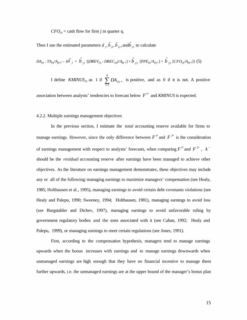
CFOjq = cash flow for firm j in quarter q.
Then I use the estimated parameters 321ˆ and,ˆ,ˆ,ˆ jjjj βββα to calculate
DAjq = TAjq/Ajq-1 – { jα̂ + 1ˆ
jβ [(∆REVjq - ∆RECjq)/Ajq-1] + 2ˆ
jβ [PPEjq/Ajq-1] + 3ˆ
jβ [CFOjq/Ajq-1]} (5)
I define KMINUSjq as 1 if ∑=
−
8
1ttjqDA is positive, and as 0 if it is not. A positive
association between analysts’ tendencies to forecast below *1F and KMINUS is expected.
4.2.2. Multiple earnings management objectives
In the previous section, I estimate the total accounting reserve available for firms to
manage earnings. However, since the only difference between *1F and *2F is the consideration
of earnings management with respect to analysts’ forecasts, when comparing *1F and *2F , −k
should be the residual accounting reserve after earnings have been managed to achieve other
objectives. As the literature on earnings management demonstrates, these objectives may include
any or all of the following: managing earnings to maximize managers’ compensation (see Healy,
1985; Holthausen et al., 1995), managing earnings to avoid certain debt covenants violations (see
Healy and Palepu, 1990; Sweeney, 1994; Holthausen, 1981), managing earnings to avoid loss
(see Burgstahler and Dichev, 1997), managing earnings to avoid unfavorable ruling by
government regulatory bodies and the costs associated with it (see Cahan, 1992; Healy and
Palepu, 1999), or managing earnings to meet certain regulations (see Jones, 1991).
First, according to the compensation hypothesis, managers tend to manage earnings
upwards when the bonus increases with earnings and to manage earnings downwards when
unmanaged earnings are high enough that they have no financial incentive to manage them
further upwards, i.e. the unmanaged earnings are at the upper bound of the manager’s bonus plan

16
(see Healy, 1985; Holthausen et al., 1995).5 Therefore, when a firm’s unmanaged earnings are
below the upper bound of the bonus plan, even if the firm has enough flexibility to manage
earnings downwards, the manager may be reluctant to do so because his or her compensation will
diminish. Consequently, the relation between unmanaged earnings and managers’ bonus plans
imposes a constraint on the relation between −k and analysts’ tendencies to forecast below *1F .
Only if the unmanaged earnings exceed the upper bound of firms’ bonus plan does forecasting
below *1F yield a smaller expected loss. Since the upper bound of firms’ bonus contract is
unobservable, I assume that the higher the unmanaged earnings are, the more likely it is for
analysts to forecast below the otherwise optimal forecast.
The political cost hypothesis introduces another constraint on the relation between −k
and analysts’ tendencies to forecast below *1F . It predicts that firms will manage high earnings
downwards to reduce political costs (Cahan, 1992; Healy and Palepu, 1999). This hypothesis has
the same implications as does the compensation hypothesis. Therefore, ceteris paribus, high
unmanaged earnings will be associated with analysts’ tendencies to forecast below *1F .
H1.2: Ceteris Paribus, the higher the firms’ unmanaged earnings are, it is more likely for
analysts’ forecasts to be below *1F .
I expect a positive correlation between UME and analysts’ tendencies to forecast below
*1F , where UME is defined as earnings minus discretionary accruals, deflated by lagged total
assets.
Previous studies have also demonstrated that debt covenant violations are costly to firms
(Healy and Palepu, 1990; Sweeney, 1994; Holthausen, 1981). If the debt covenant is binding,
though firms may have the flexibilities to manage earnings downwards, they will choose not to do
5 Healy (1985) argues that managers will also manage earnings downwards when unmanaged earnings are significantly below the lower bound of the compensation contract. However, the findings in both Gaver et al. (1995) and Holthausen et al. (1995) suggest that this result is driven by the research design.

17
so. Therefore, ceteris paribus, firms are less likely to manage earnings downwards when debt-
covenants are binding.
H1.3: Ceteris Paribus, the lower the firms’ debt to equity ratios are, it is more likely for
analysts’ forecasts to be below *1F .
To test this hypothesis, I calculate debt to equity ratio, DEjq, as total debt divided by total
equity. A negative relation between DE and analysts’ tendencies to forecast below the otherwise
optimal forecast is expected.
Finally, Burgstahler and Dichev (1997) provide evidence that firms have incentives to
manage earnings upwards to avoid losses. They also demonstrate that when a firm does not have
the accounting flexibility to report a profit, it will choose to manage the earnings downwards,
reporting a large loss, so that it can save accounting reserve for future use. Therefore, firms are
more likely to manage earnings downwards when reporting loss is inevitable. Based on
Burgstahler and Eames (1998)’s evidence that analysts anticipate firms’ earnings management to
avoid loss, I use the sign of analysts’ forecasts as an indicator of whether or not the loss is
unavoidable . Analysts only release negative forecasts when they believe that firms cannot avoid
losses.
H1.4: Ceteris Paribus, for firm-quarters in which analysts’ earnings forecasts are losses,
analysts’ forecasts are more likely to be below *1F .
I create a dummy variable LOSSjq. LOSSjq equals to 1 when Fjq is negative, and 0
otherwise. I predict that there is a positive correlation between LOSS and analysts’ tendencies to
forecast below *1F .
4.3. SKEWNESS OF EARNINGS DISTRIBUTION
As stated in H2, for firm-quarters whose distributions of unmanaged earnings are
negatively skewed, the expected loss will be lower if analysts forecast below *1F .

18
The skewness is estimated using the skewness metric,
∑ −−−
= 3)/)(()2)(1( jjjq
jj
jjq sUMEUME
nn
nSKEW ,
6 (6)
where UMEjq is unmanaged earnings for firm j at quarter q.7 jUME is the mean, js is the
standard deviation, and jn is the number of observations of firm j’s UME within the relevant
rolling window. Following Gu and Wu (2003), the rolling window includes observations from
quarters q-8 to q-1 and quarters q+1 to q+8, and requires a minimum of four observations in each
segment.8 I predict that the more negative SKEWjq is, the more likely it is for analysts to forecast
below *1F .
4.4. ANALYSTS’ FORECASTS
The previous sections assume that analysts do not revise their forecasts. However, at least
one third of analysts’ forecasts in my sample have been revised (see section 5) after they were
released. There is also evidence (see Matsumoto, 2002) that on average, analysts revise their
forecasts downwards. In the test I divide the forecast data into two sets, one comprising forecasts
that were not revised and the other forecasts that were. From these two data sets, I am able to test
three analysts’ consensus forecasts: 1) the median of the forecasts that were not revised,
F_NOREVISE; 2) the median of forecasts which that were later revised, F_ORIGINAL; and 3) the
median of the revised forecasts after their final revision, F_FINAL. Testing these three consensus
forecasts separately will enable me to demonstrate that analysts consider earnings management
when generating their forecasts, regardless of further revision.
6 Another measurement of skewness, the mean and median difference of earnings, is also used, and generates similar results. 7 Using realized EPS doesn’t change the result. 8 As a sensitive test, I try to calculate skewness metrics in 2 other different rolling windows. One includes observations from quarter q-8 to q-1 only, and the other includes all the observations from quarter q-8 to quarter q+8. The results remain unchanged.

19
In the test I assume that analysts always try to make accurate forecasts, and that analysts
only revise their forecasts when they believe they have new or more accurate information that
will allow them to make better forecasts. Hence, ex ante, when analysts release F_ORIGINAL,
they do not foresee that they will revise their forecasts. Therefore, I predict that F_ORIGINAL
will have characteristics similar to F_NOREVISE, and that these two groups will generate similar
results in my hypotheses tests.
Since the forecasts in F_FINAL are based on updated information, I predict that
F_FINAL will be more accurate than F_NOREVISE and F_ORIGINAL. As for the bias in the
forecasts, although on average, the forecasts have been revised downwards, I assume that revision
of the forecasts does not alter either analysts’ concerns with forecasting accurately or the attention
they pay to firms’ earnings management behavior. Between F_NOREVISE and F_ORIGINAL on
the one hand and F_FINAL on the other, the only difference that might impact analysts’ decision-
making is that the forecasting period following F_FINAL’s release is much shorter than that
following the release of the other two forecasts. Since the earnings announcement date is
approaching following F_FINAL’s release, the opportunity for firms to manipulate discretionary
accruals diminishes. In addition, as time passes, analysts may gain insight into firms’ tendencies
and flexibilities to manage earnings other than previous accounting report. Because the proxies in
my tests are mainly based on previous quarters’ accounting information, and do not reflect the
fresh information available to analysts as the earnings announcement date approaches, the
possibility of measurement error increases, and this will weaken test results.
Based on H1 and H2, I predict that the consensus forecasts will be systematically lower
than the otherwise optimal forecast for firm-quarters with negatively skewed earnings
distributions and with higher tendencies and flexibilities to manage earnings downwards. Each
consensus forecasts, F_NOREVISE, F_ORIGINAL, and F_FINAL, will generate similar results.
However, I predict that F_FINAL will generate the weakest result.

20
4.5. CONTROL VARIABLES
Following prior research, 9 I include several variables in my test to control for other
factors that might contribute to analysts’ tendencies to forecast below or above *1F .
First, because Brown (1997) finds that analysts’ forecasts exhibit less optimistic bias for
larger firms, I control for size using the log of the equity’s market value at the end of the previous
quarter, LOGMVjq-1. I predict that the correlation between LOGMV and analysts’ tendencies to
make lower forecasts will be positive.
Second, I consider analyst following as a variable related to forecast bias. The nature of
this relation, however, remains an open question. Lim (2001) finds evidence that proxies for the
richness of a company’s information environment, including analyst following, are inversely
related to optimistic bias in forecasts. The reason is that analysts temper their optimistic bias to
gain access to management. Gu and Wu (2003), on the other hand, argue that the number of
analysts following is positively correlated with optimistic bias. A greater degree of analyst
following, according to Gu and Wu, indicates intense competition, and will drive analysts to issue
increasingly optimistic forecasts in order to compete for management favor. Because the effects
of analyst following are still unclear, I make no predictions here regarding this factor. I use the
natural log of the number of analysts making quarterly forecasts (LOGAFjq) as a proxy for analyst
following.
Two additional variables are used to proxy for uncertainty in the forecasting environment.
These two variables are forecast dispersion (FDISPiq), and variation of EPS (EVARiq). FDISPiq is
defined as the standard deviation of forecasts deflated by lagged price. The forecasts must be
released between the previous earnings announcement date and the current earnings
announcement date. EVARiq is measured as the standard deviation of EPS divided by the absolute
value of the mean EPS, within the same rolling window as which the SKEWiq is measured. Since
9 Most of the control variables are similar to the ones used by Gu and Wu (2003). The relation between this research and Gu and Wu (2003) is discussed in detail in section 2.2.

21
FDISP and EVAR are correlated with firm size , no clear prediction can be made as to how these
variables correlate with analysts’ tendencies to forecast below or above *1F .
Finally, according to Abarbanell and Bernard (1992), analysts tend to underreact to recent
earnings surprises. I control for this underreaction by adding the variables RWSUR_1jq and
RWSUR_2jq. These two variables are lagged-price-deflated lag-one and lag-two earnings surprises
measured using a random walk model. I predict a positive relation between RWSUR and
analysts’ tendencies to forecast below *1F .
Because the magnitude of forecasting below *1F is not necessarily correlated linearly
with all of the variables I have described, I use a logit model. I classify firm-quarters as
forecasted below *1F (LOWER jq =1) if the consensus forecast is lower than the earnings
prediction generated by the LAD method, or as forecasted above *1F (LOWER jq =0) if not. The
logit regression is as follows:
Prob {LOWER_i jq = 1}
= F (?0 + ?1 KMINUSjq + ?2 UMEjq + ?3 DEjq + ?4LOSS_ijq + ?5SKEWjq
+ ?6 LOGMVjq-1+ ?7 LOGAFjq+ ?8 FDISPjq+ ?9 EVARjq
+ ?10RWSUR_1jq+ ?11 RWSUR_2jq) (7)
where:
X
X
ee
X'
'
1)'(F
γ
γ
γ+
=
i = NOREVISE, ORIGINAL or FINAL
5. Data and Descriptive Statistics
5.1. DATA
Earnings per share, excluding extraordinary items and other accounting variables have
been obtained from the 2001 COMPUSTAT quarterly industrial and research files. The sample

22
period is from 1987 to 2001. I choose to start from 1987 because the data on cash flow from
operations reported in the statement of cash flows, which are necessary for calculating
discretionary accruals, are only available from 1987. Previous research (Jones, 1990; Dechow et
al., 1995) use balance sheet data to calculate cash flow from operations, but as Collins and Hribar
(2000a) point out, such an approach can introduce measurement errors. Therefore, I limit my data
to the 1987 to 2001 period, using cash flows from operations excluding extraordinary items and
discontinued operations (COMPUSTAT data item #108 minus data item #78) to calculate
accruals and discretionary accruals.10
I also restrict my analysis to firms that do not have any missing data for the variables
used in the empirical analysis. In order to estimate both the Foster model using the LAD method
and the modified Jones’ model in a rolling window for each firm-quarter, I must first estimate the
necessary parameters. To make these preliminary estimations, I require that for each firm-quarter,
there must be at least 10 consecutive observations prior to that quarter. I further eliminate
observations with SIC codes 4400-5000 and 6000-6999. These codes correspond to the utility and
financial service industries whose earnings predictions are quite different from others.
Analysts’ forecasts are obtained from 2001 Zacks Investment Research database. In order
to ensure that analysts have all of the previous quarters’ accounting information, I use only those
forecasts that follow the previous quarters’ earnings announcement.
As discussed in section 4.4, I divide the Zacks forecast data into two sets, one composed
of forecasts that have not been revised, and the other containing forecasts that have, and then
merge each set separately with the COMPUSTAT data. The criteria I have described generate a
no-revising-forecasts sample with 17,870 firm-quarter observations, representing 1,794 firms, and
a revising-forecasts sample with 11,377 firm-quarter observations, representing 1,514 firms.
10 See Collins and Hribar (2000b). If data78 is missing, I assume it is 0.

23
5.2. DESCRIPTIVE STATISTICS
Table 2 represents the descriptive statistics for several key variables. Consistent with
prior studies (Kazsnik and McNichols, 1999; Lys and Sohn, 1991), earnings surprises have
negative means (-0.16% of lagged stock price for earnings surprises with respect to
F_NOREVISE, -0.31% with respect to F_ORIGINAL, and -0.13% with respect to F_FINAL), and
positive medians (0.10% of lagged stock price for surprises with respect to F_NOREVISE, 0.09%
with respect to F_ORIGINAL, and 0.13% with respect to F_FINAL). These statistics suggest that
majority of the firms in the sample beat analysts’ forecasts, and that the negative surprises have
larger absolute values than positive surprises.
As predicted, F_FINAL is the most accurate forecasts, with an average forecasting
horizon of 27 days, and mean absolute forecast error of 1.11% of lagged stock price.
F_ORIGINAL is the least accurate forecasts among the three consensus forecasts, with an mean
absolute forecast error of 1.24% of lagged stock price. Other descriptive statistics show that the
firms whose forecasts are most frequently revised are larger firms with more analysts following
and less variable earnings. Hence, even though F_ORIGINAL is made for firm-quarters with a
better forecast environment, the longer forecasting horizon (79 days vs. 55 days of F_NOREVISE)
causes it to be less accurate than F_NOREVISE, which has an mean absolute forecast error of
1.18%.
6. Empirical results
6.1. IS IT POSSIBLE FOR FIRMS TO TAKE A BIG BATH?
One of the premises for my hypotheses is that firms may manage earnings downwards
when forecasts cannot be met or beaten, and the anticipation of this downward earnings
management induces analysts to forecast below *1F . The frequency of downward earnings
management provides some preliminary evidence for this claim. Of the 7,899 firm-quarters in

24
which unmanaged earnings fail to meet F_NOREVISE11 , 1,059 firm-quarters, approximately
13.5%, realize negative discretionary accruals when earnings are announced, i.e., have managed
earnings downwards. On average, discretionary accruals of these 1,059 firm-quarters’ are -2% of
total assets, or approximately negative 60 million dollars per firm. Therefore, firms are likely to
take a big bath when analysts’ forecasts cannot be met without earnings management, and there is
evidence that many firms have done so.
6.2. EARNINGS PREDICTION
Before formally testing my hypotheses, I will assess the validity of my claim that
earnings predictions estimated by the LAD method are more accurate than those generated by the
least squares method. For each firm-quarter, I calculate three different lagged-price-deflated
absolute forecast errors (ABSUR_LADjq, ABSUR_FOSTERjq, and ABSUR_BRjq) by calculating the
absolute difference between EPS jq and earnings predictions generated by one of the following
three method: Foster prediction using the LAD method, Foster prediction using the least squares
method, and Brown and Rozeff prediction using the least squares method. For firm-quarters with
forecasts that have not been revised, ABSUR_LAD has a mean of 1.68% of lagged stock price,
which is significantly smaller than the 1.89% generated by ABSUR_FOSTER, and the 1.87%
derived from ABSUR_BR.12 For firm-quarters with revised forecasts, the results are similar.
Therefore, as predicted, earnings predictions estimated by the LAD method have a smaller mean
absolute forecast error than those estimated by the least squares method.
11 Use F_ORIGINAL and F_FINAL, the percentage are approximately the same. 12 The t-statistics for the null hypothesis that mean (ABSUR_LAD) is bigger than mean (ABSUR_FOSTER) is -2.81. The null hypothesis is rejected at 1% confident level. The t-statistics for the null hypothesis that mean (ABSUR_LAD) is bigger than mean (ABSUR_BR) is -2.69. The null hypothesis is rejected at 1% confident level.

25
6.3. TEST OF HYPOTHESES --- LOGIT MODEL
Tables 4 and 5 show the descriptive statistics and the regression results of the logit model
(equation 7). Panel B reports the Pearson (above the diagonal) and the Spearman (below the
diagonal) correlations among the variables used to estimate equation (7). As predicted, analysts’
tendencies to forecast below *1F , as measured by LOWER_i, is significantly posit ively
associated with KMINUS, UME and LOSS_i, and is significantly negatively associated with DE
and SKEW. The positive correlation between LOWER_i and KMINUS suggests that analysts are
more likely to forecast below *1F during firm-quarters when firms have more flexibility to
manage earnings downwards. The level of unmanaged earnings, UME, is positively correlated
with LOWER_i, indicating that analysts are more likely to forecast below *1F for firm-quarters
with higher unmanaged earnings , in anticipation of downward earnings management by firms.
LOSS_i is also positively associated with LOWER_i, providing evidence that analysts anticipate
firms’ big bath behavior when losses are inevitable . The fact that LOWER_i is negatively
correlated with DE suggests that, for firm-quarters with binding debt covenants, it is less likely
earnings will be managed downwards. As a result, analysts do not need to forecast below *1F .
Finally, the negative association between LOWER_i and SKEW provides evidence that supports
H2, i.e., for firm-quarters with earnings belonging to a negatively skewed distribution, analysts
tend to forecast below *1F because doing so generates a lower expected loss. Taken together, the
univariate analysis indicates that analysts consider firms’ earnings management when shaping
their forecasts, and that it is not necessarily optimal for them to forecast *1F .
The analysis also suggests several significant correlations among independent variables.
For example , SIZE is correlated with most of the variables. Larger firms tend to have lower debt
to equity ratio, more analyst following, and less variable earnings. Though several of these
correlations are statistically significant, the magnitudes of most correlations have absolute values
26
less than 0.2, suggesting that multi-colinearity is not an issue. 13 Since omitting any of the
independent variables will lead to an omitted correlated variables problem, I incorporate all of
them in the logit model.
As predicted by H1 and H2, whichever consensus forecasts are used, DOWN, UME, DE,
LOSS_i, and SKEW have significant coefficients, and all of which are in the predicted direction.
These results suggest that analysts are more likely to forecast below *1F for those firm-quarters
with higher accounting reserves, with higher unmanaged earnings, with non-binding debt
covenants, with negative forecasted earnings, and with negatively skewed unmanaged earnings.
Also notice that among the three forecasts, F_FINAL generates the weakest result, with the
smallest log likelihood chi-square, and the smallest marginal effect on variable DOWN, UME,
and DE. This weak result reflects the fact that as the earnings announcement date approaches,
analysts sometimes have additional information about whether firms are likely to manage
earnings downward. The additional information available to analysts weakens the relation
between the deviation of forecasts and the variables based only on previous accounting
information.
As for the control variables, the coefficient of LOGAF is insignificant at conventional
levels, suggesting that analyst following is not a factor associated with analysts’ bias. This is not
surprising insofar as previous studies offer mixed results. FDISP has a significantly negative
coeffic ient, indicating that analysts tend to forecast lower when the forecast dispersion is low.
EVAR does not have a significant coefficient. The proxies for analysts’ underreaction to firms’
previous performance do not have significant coefficients either.
13 When I conduct sensitive test using OLS model (section 6.5), I test the multicollinearity using the Variance Inflation Factor (VIF) method. The variance inflation values also indicate that multicollinearity is not a concern.

27
6.4. ASYMMETRIC DISTRIBUTION OF EARNINGS SURPRISES
In this section, I analyze the distribution of earnings surprises. According to previous
studies, earnings management that responds to analysts’ forecasts causes an asymmetric
distribution of earnings surprises. That is, more firms beat analysts’ forecasts than fail to do so.
There are a disproportionately large number of positive earnings surprises and a
disproportionately small number of negative earnings surprises. Since earnings surprises depend
upon two variables, earnings and analysts’ forecasts, one variable must be fixed in order to draw a
valid conclusion about the other. My hypotheses indicate that analysts predict firms’ earnings
management behavior. Therefore, the studies that analyze earnings surprises mix the effect of
analysts’ precaution of earnings management and that of firms’ realized earnings management
behavior together. By comparing earnings surprises with respect to analysts’ forecasts and
earnings surprises with respect to forecasts generated by a statistical model, it becomes clear that
analysts’ forecasts likely contribute to the asymmetric distribution of earnings surprises.
First, for the 17,870 firm-quarters with forecasts that have not been revised, 11,082 firm-
quarters, approximately 62.01%, have earnings per share that meet or beat F_NOREVISE; while
only 9,209, approximately 51.03%, have earnings per share that meet or beat EPS_LAD. Similar
statistics appear when I use the revised-forecasts sample. The pessimistic bias, hence, is more
pronounced for the analysts’ forecasts, than for the statistical-model-generated forecasts.
Figure 1 presents distributions of earnings surprises over a range of lagged-price-deflated
earnings surprises, from – 2% of lagged stock price to 2% of lagged stock price.14 Panel A shows
that the distribution of earnings surprises defined with respect to the median forecast
(F_NOREVISE15 ), and Panel B presents the distributions of earnings surprises defined with
respect to the earnings prediction generated by the LAD method. Panel A shows a pattern of low
frequency to the left of zero and high frequency immediately to the right of zero. This pattern
14 See Burgstahler and Eames (1998). 15 Using F_ORIGINAL, F_FINAL generates similar figures, not reported here.

28
closely resembles the results of previous studies. Such a pattern, however, does not exist in Panel
B. The standardized difference for the first interval left of zero is used to assess the significance
of the asymmetric distribution. 16 Using analysts’ forecast to calculate earnings surprises, the
standardized difference for the interval is -16.71, significant at the 0.0001 level. However, using
statistical model generated forecast, the standardized difference for the interval immediately left
of zero is only -0.28, insignificant at conventional levels.
These figures and statistics suggest that the pattern of asymmetric distribution, which is
prominent when analysts’ consensus forecasts are used, disappears when predictions generated by
the statistical models are used. Therefore, analysts’ behavior likely contributes to the asymmetric
distribution of earnings surprises.
6.5. SENSITIVITY TESTS
I conducted additional tests for sensitivity analyses. First, the logit model (equation 7)
only indicates the probability of analysts forecasting below the Foster prediction generated by the
LAD method, but it does not generate any information about the magnitude of analysts’ forecasts’
deviation from *1F . Therefore, I ran an OLS regression using the logit model’s independent
variables as independent variables, and the difference between the proxy of *1F and the
consensus forecasts as dependent variables.
DELTA_ijq
= ? 0 + ? 1 KMINUSjq + ? 2 UMEjq + ? 3 DEjq + ? 4LOSS_ijq +? 5SKEWjq
+ ? 6 LOGMVjq-1+ ? 7 LOGAFjq+ ? 8 FDISPjq+ ? 9 EVARjq
16Following Burgstahler and Dichev (1997), the standardized difference is defined as the difference between the actual and expected number of observations in an interval, divided by the estimated standard
deviation of the difference. Denoting the probability that an observation will fall into interval i by ip , the
expected number of observations in interval I is 2
* 11 +− + ii ppN , and the variance of the difference between
the observed and expected number of observations for interval I is approximately
4))(1(*)(
*)1(** 1111 +−+− +−++− iiii
ii
ppppNppN .

29
+ ? 10 RWSUR_1jq+ ?11RWSUR_2jq (8)
where DELTA_ijq = EPS_LADjq – F_ijq
i = NOREVISE, ORIGINAL and FINAL
As before, the estimated coefficients of KMINUS , UME, and LOSS_i are predicted to be
positive, and those of SKEW and DE are predicted to be negative. Generally, the bigger the
KMINUS are, and / or the higher the unmanaged earnings are, and/or the more likely losses are
inevitable, the more likely analysts are to forecast below *1F . Analysts also have stronger
reasons to forecast below *1F when firm-quarters have negatively skewed unmanaged earnings,
and/or firm-quarters’ debt covenants are not binding. The results are reported in Table 6. All the
estimated coefficients have the predicted sign, though several of them, including SKEW and UME,
are not significant, suggesting that the relation between the dependent variable and these
independent variables is not necessarily linear.
Gleason and Lee (2003) point out that multiple observations from the same firm could
result in correlation among errors in one equation, leading to inaccurate statistics. In order to
correct for this, I run the logit model (equation 7) using a sub-sample. In the sub-sample, for each
firm, only the data from the most current quarter are included. The results are consistent with
those in the earlier test.
I conduct several other sensitivity checks. The results are unchanged when I use the
traditional Foster predictions and Brown and Rozeff predictions as proxies for *1F . I also try
different discretionary accruals models (see Thomas and Zhang, 2000), and use the most recent
forecasts instead of the consensus forecasts, and use total assets as deflators in the analysis.
Similar results are obtained for each case.
30
7. Conclusion
Previous earnings management studies suggest that firms manage earnings to meet or to
beat analysts’ earnings forecasts. The evidence shows that earnings surprises are asymmetrically
distributed; that is, more firms beat analysts’ forecasts than fail to do so. There are a
disproportionately large number of small positive earnings surprises. However, analysts’ forecasts
literature tends to ignore that firms’ earnings management practices respond to analysts’ forecasts.
This study investigates the properties of analysts’ earnings forecasts by hypothesizing
that analysts are aware of the earnings management practices of firms, and incorporate such
behavior into their forecasts. Under these assumptions, forecasting either below or above the
otherwise optimal forecast can lower analysts’ expected loss. For firms that have greater abilities
/ tendencies to manage earnings downwards, negatively skewed unmanaged earnings, or both,
forecasting lower than the median can produce a lower expected loss. Similarly, forecasting
higher than the median can generate a lower expected loss for firms that have the capacities to
manage earnings upwards, positively skewed unmanaged earnings, or both.
Using the quarterly consensus forecasts data and accounting data from 1987 to 2001, I
provide evidence that the higher the flexibility firms have to manage earnings downwards, the
higher the unmanaged earnings are, the less likely debt covenants are to be violated, the more
likely losses are inevitable, and/or the more negatively skewed the unmanaged earnings are, the
more likely the analysts will forecast lower than the otherwise optimal forecasts. There is also
evidence that the analysts’ efforts to avoid big bath practices by firms contribute to the
asymmetric distribution of earnings surprises.
This paper also raises a couple of important questions for future research. First, I have
only demonstrated that under certain circumstances, the assumption that analysts consider
earnings management leads to a different optimal forecast. However, I do not solve for the
optimal forecast. Second, I consider analysts’ forecasts as analysts’ strategic responses to

31
predicted firms’ behavior. After observing analysts’ forecasts, firms’ actual behavior is also worth
investigating. For example, it would be interesting to examine why some firms would like to
issue their own forecasts after observing the analysts’ forecasts.
32
References Abarbanell, J. and V. Bernard. “Tests of Analysts’ Overreaction/Underreaction to Earnings
Information as an Explanation for Anomalous Stock Price Behavior.” Journal of Finance 47 (1992): 1181-1207.
Abarbanell, J. and R. Lehavy. “Biased Forecasts or Biased Earnings?” Working paper (2000),
University of North Carolina. Barth, M., D.P. Cram, and K. Nelson. “Accruals and the Predictions of Future Cash Flows.” The
Accounting Review 76 (2001): 27-58. Bartov, E., D. Givoly, and C. Hayn. "The Rewards for Meeting-or-Beating Earnings
Expectations." Journal of Accounting and Economics 33 (2002): 173 – 204. Basu, S. “The Conservatism Principle and the Asymmetric Timeliness of Earnings.” Journal of
Accounting and Economics 24 (1997) 3-37. Basu, S, and S. Markov. “Loss Function Assumptions in Rational Expectations Tests on Financial
Analysts’ Earnings Forecasts.” Working paper (2003) Emory University. Bhushan, R. “Firm Characteristics and Analyst Following.” Journal of Accounting and
Economics 11 (1989): 255-274. Birkes, D. and Y. Dodge Alternative Methods of Regression. (1993) New York: John Wiley &
Sons. Brown, L. “Earnings Forecasting Research: Its Implications for Capital Markets Research.”
International Journal of Forecasting 9 (1993):295-320. Brown, L. “Analyst Forecasting Errors: Additional Evidence.” Financial Analysts’ Journal 53
Nov/Dec. (1997): 81-88.
Brown, L., R.Hagerman, P.Griffin, and M. Zmijewski. “An Evaluation of Alternative Proxies for the Market’s Assessment of Unexpected Earnings.” Journal of Accounting and Economics 9 (1987): 159-193.
Brown, L., and M. Rozeff. “Univariate Time-Series Models of Quarterly Accounting Earnings per Share: A Proposed Model.” Journal of Accounting Research 17 (1979):179-189.
Burgstahler, D. and I. Dichev. “Earnings Management to Avoid Earnings Decreases and Losses.”
Journal of Accounting and Economics 24 (1997):99-126. Burgstahler, D. and M. Eames. “Management of Earnings and Analyst Forecasts.” Working
Paper (1998), University of Washington. Cahen, S. “The Effect of Antitrust Investigations on Discretionary Accruals: A Refined Test of
the Political-Cost Hypothesis.” The Accounting Review 67 (1992): 77-95.

33
Chaney, K., D. Jeter, and M. Lewis. “The Use of Accruals in Income Smoothing: A Permanent Earnings Hypothesis.” Advances in Quantitative Analysis of Finance and Accounting 6 (1999): 103-135.
Chevis, G., S. Das, and K. Sivaramakrishnan. “An Empirical Analysis of Firms that Meet or
Exceed Analysts’ Earnings Forecasts.” Working Paper (2001), Texas A&M University. Collins, D. and P. Hribar. “Errors in Estimating Accuruals: Implications for Empirical Research.”
Working Paper (2000), University of Iowa. Collins, D. and P. Hribar. “Earnings-Based and Accrual-Based Market Anomalies: One Effect or
Two?” Journal of Accounting and Economics 29 (2000): 101-123. Das, S., C. Levine, and K.Sivaramakrishnan. “Earnings Predictability and Bias in Analysts’
Earnings Forecasts.” The Accounting Review 73 (1998): 277-294. Dechow, P. “Accounting Earnings and Cash Flows as Measures of Firm Performance” Journal of
Accounting and Economics 18 (1994): 3-42. Dechow, P., S.P. Kothari, and R. Watts. “The Relation between Earnings and Cash Flows.”
Journal of Acounting and Economics 25 (1998): 133-168. Dechow, P., R. Sloan, and A. Sweeney. “Detecting Earnings Management.” The Accounting
Review 70 (1995): 193-225. Dechow, P., S. Richardson, and I. Tuna. “Are Benchmark Beaters Doing Anything Wrong?”
Working paper (2000), University of Michigan. Degeorge, F., J. Patel, and R. Zeckhauser. “Earnings Management to Exceed Thresholds.”
Journal of Business 72 (1999): 1-33. Demski, J. and G.Feltham. “Forecast Evaluation” The Accounting Review (1972): 533-548. Foster, G. Financial Statement Analysis (1986) Prentice Hall. Foster, G. “Quarterly Accounting Data: Time-Series Properties and Predictive Ability Results.”
The Accounting Review 52 (1977): 1-21. Francis, J. and D. Philbrick. “Analysts’ Decisions as Products of a Multi-Task Environment.”
Journal of Accounting Research 31 (1993): 216-230. Gaver, J., K. Gaver, and J. Austin. “Additional Evidence on Bonus Plans and Income
Manangement.” Journal of Accounting and Economics 18 (1995):3-28. Givoly, D., and C. Hayn. “The Changing Time-Series Properties of Earnings, Cash Flows and
Accruals: Has Financial Reporting Become More Conservative?” Journal of Accounting and Economics 29 (2000): 287-320.
Gleason,C.A., and C.M.C.Lee. “Analyst Forecast Revisions and Market Price Discovery.” The
Accounting Review 78 (2003): 193-226.

34
Griffin, P. “The Time-Series Behavior of Quarterly Earnings: Preliminary Evidence.” Journal of Accounting Research 15 (1977): 71-83.
Gu, Z and S. Wu. “Earnings Skewness and Analysts’ Forecasts Bias.” Journal of Accounting and
Economics 35 (2003): 5-29. Healy, P. “The Effect of Bonus Schemes on Accounting Decisions.” Journal of Acounting and
Economics 7 (1985): 85-107. Healy, P. and K. Palepu. “The Effectiveness of Accounting-Based Dividend Covenants.” Journal
of Accounting and Economics 12 (1990): 97-123. Healy, P. and K. Palepu. “A Review of the Earnings Management Literature and its Implications
for Standard Setting.” Accounting Horizons 13 (1999): 365-383. Holthausen, R. “Evidence on the Effect of Bond-Covenants and Management Compensation
Contracts on the Choice of Accounting Techniques.” Journal of Accounting and Economics 3 (1981): 73-109.
Holthausen, R., D. Larcker, and R. Sloan. “Annual Bonus Schemes and the Manipulation of
Earnings.” Journal of Accounting and Economics 19 (1995):29-74. Hwang, L., C. Jan, and S. Basu “Loss Firms and Analysts’ Earnings Forecast Errors.” Journal of
Financial Statement Analysis 1 (1996): 18-30. Jones, J. “Earnings Management During Import Relief Investigations.” Journal of Accounting
Research 29 (1991): 193-228. Kasznik, R. and M. McNichols. “Does Meeting Expectations Matter? Evidence from Analysts
Forecast Revisions and Share Prices.” Working paper (1999), Stanford University. Kothari, S. P. “Capital Markets Research in Accounting.” Journal of Accounting and Economics
31(2001): 105-231. Lim, T. “Rationality and Analysts’ Forecast Bias.” Journal of Finance 56 (2001):369-385. Lopez, T. and L. Rees. “The Effect of Beating and Missing Analysts’ Forecasts on the Information
Content of Unexpected Earnings.” Journal of Accounting, Auditing, and Finance 17 (2002): 155-184.
Lys, T. and S. Sohn. “The Association Between Revisions of Financial Analysts’ Earnings
Forecasts and Security-Price Changes.” Journal of Accounting and Economics 13 (1990): 341-363.
Matsumoto, D. “Management's Incentives to Avoid Negative Earnings Surprises” The
Accounting Review 77 (2002): 483-514. McNichols, M. “Research Design Issues in Earnings Management Studies.” Journal of
Accounting and Public Policy 19 (2000): 313-345.
35
McNichols, M. and P. O’Brien. “Self-Selection and Analyst Coverage.” Journal of Accounting Research (Supplement 1997): 167-199.
O’Brien, P. “Analysts’ Forecasts as Earnings Expectations.” Journal of Accounting and
Economics 10 (1988): 53-83. O’Brien, P. and R. Bhushan. “Analyst Following and Institutional Ownership.” Journal of
Accounting Research (Supplement 1990): 55-82. Skinner,D., and R. Sloan. “Earnings Surprises, Growth Expectations and Stock Returns.”
Working Paper (1999), University of Michigan. Sloan, R. “Do Stock Prices Fully Reflect Information in Accruals and Cash Flows about Future
Earnings?” The Accounting Review 71 (1996): 289-315. Subramanyam K.R. “The Pricing of Discretionary Accruals” Journal of Accounting and
Economics 22 (1996): 249-281. Sweeney, A. “Debt-Covenant Violations and Managers’ Accounting Responses.” Journal of
Accounting and Economics 17 (1994): 281-308. Thomas, J. and X. Zhang. “Identifying Unexpected Accruals: a Comparison of Current
Approaches.” Journal of Accounting and Public Policy 19 (2000): 347-376. Watts, R. “The Time-Series Behavior of Quarterly Earnings.” Working paper (1975), University
of Newcastle.

36
Appendix 1
Conditions under which the optimal forecast changes when earnings management (meet or slightly beat analysts’ forecasts) is considered Let *1F be the optimal forecast before considering earnings management. Let *2F be the optimal forecast assuming the firm want to meet or slightly beat the analyst’s forecast, i.e., *2F minimizes
(1) )()()()()()( 1 ∫∫∫∞
+
−+
−
−
∞−
−
−
−
+
+
−−++++−=kF
kF
kF
kF
dxxfFkxLdxxfdxxfFkxLLE ε
where 0,0,0 ≥′′>′≥ LLL
Since *1F minimizes the expected loss before considering earnings management, one can adjust F = *1F up or down to see the effect on 1)(LE . In equation (1) , suppose e is arbitrarily small.
Now compare the first term dxxfFkxLkF
)()(∫+−
∞−
− ++− and the last term
∫∞
+
−
−
−−kF
dxxfFkxL )()( .
0)()()()()()(
>=++−′+−+++−=∂
++−∂
∫∫ +
+
−
∞−
−+−+
−
∞−
−
dxxfFkxLkFfFkkFLF
dxxfFkxLkF
kF
Q
0)()(')()(
)()(
, <=−−−+−−+−=∂
−−∂
∫∫ ∞
+
−−−−
∞
+
−
−
−
kF
kF dxxfFkxLkFfFkkFLF
dxxfFkxL
Also
∴ The first term dxxfFkxLkF
)()(∫+−
∞−
− ++− is increasing in F, while the last term
∫∞
+
−
−
−−kF
dxxfFkxL )()( is decreasing in F.
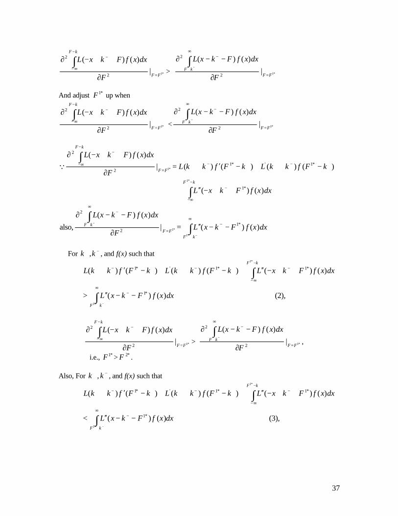
Therefore, in order to minimize equation (1), one needs to adjust *1F down when
37
*1|)()(
2
2
FF
kF
F
dxxfFkxL
=
−
∞−
−
∂
++−∂ ∫+
> *1|
)()(
2
2
FFkF
F
dxxfFkxL
=
∞
+
−
∂
−−∂ ∫−
And adjust *1F up when
*1|)()(
2
2
FF
kF
F
dxxfFkxL
=
−
∞−
−
∂
++−∂ ∫+
< *1|
)()(
2
2
FFkF
F
dxxfFkxL
=
∞
+
−
∂
−−∂ ∫−
dxxfFkxL
kFfkkLkFfkkLF
dxxfFkxL
kF
FF
kF
)()(
)()()()(|)()(
*1
*1
*1
*1'*12
2
∫
∫
+
+
−
∞−
−
+−++−+=
−
∞−
−
++−′′+
−++−′+=∂
++−∂Q
∫∫ ∞
+
−=
∞
+
−
−
−
−−′′=∂
−−∂
kFFF
kF dxxfFkxLF
dxxfFkxL
*1
*1 )()(|
)()(
also, *12
2
∴ For +k , −k , and f(x) such that
,(2) )()(
)()( )()()()(
*1
*1
*1
*1*1'*1
∫
∫∞
+
−
−
∞−
−+−++−+
−
+
−−′′>
++−′′+−++−′+
kF
kF
dxxfFkxL
dxxfFkxLkFfkkLkFfkkL
*1|)()(
2
2
FF
kF
F
dxxfFkxL
=
−
∞−
−
∂
++−∂ ∫+
> *1|
)()(
2
2
FFkF
F
dxxfFkxL
=
∞
+
−
∂
−−∂ ∫−
,
i.e., *1F > *2F . Also, For +k , −k , and f(x) such that
,(3) )()(
)()( )()()()(
*1
*1
*1
*1*1'*1
∫
∫∞
+
−
−
∞−
−+−++−+
−
+
−−′′<
++−′′+−++−′+
kF
kF
dxxfFkxL
dxxfFkxLkFfkkLkFfkkL

38
*1|)()(
2
2
FF
kF
F
dxxfFkxL
=
−
∞−
−
∂
++−∂ ∫+
< *1|
)()(
2
2
FFkF
F
dxxfFkxL
=
∞
+
−
∂
−−∂ ∫−
,
i.e., *1F < *2F . Without specifying the exact form of f(x) and L, from inequality (2) and (3), one can see that:
When −k is big, and / or f(x) is negatively skewed, it is more likely that
*1|)()(
2
2
FF
kF
F
dxxfFkxL
=
−
∞−
−
∂
++−∂ ∫+
> *1|
)()(
2
2
FFkF
F
dxxfFkxL
=
∞
+
−
∂
−−∂ ∫−
, i.e., *1F >
*2F .
Also, When +k is big, and / or f(x) is positively skewed, it is more likely that
*1|)()(
2
2
FF
kF
F
dxxfFkxL
=
−
∞−
−
∂
++−∂ ∫+
< *1|
)()(
2
2
FFkF
F
dxxfFkxL
=
∞
+
−
∂
−−∂ ∫−
, i.e., *1F <
*2F .
For example, consider the two most commonly used Loss function, L(y) = |y| and L(y) = |y|2.
1. L(y) = |y| The analyst’s objective is to minimize the mean absolute forecast error. Without considering earnings management with respect to analysts’ forecast, the optimal forecast
*1F is the median of the earnings’ distribution (xm) (see Gu and Wu, 2003). The inequality (2) then will take the form of:
)()()()( −++−+ +>−+−′+ kxfkxfkxfkk mmm 1.1. Suppose x is normally distributed,
)()( +−+ −′+ kxfkk m > 0,
In addition, if −k > +k , )()( −+ +>− kxfkxf mm .
∴For firms with −k > +k , *1F > *2F . 1.2. Suppose x is negatively skewed
e.g., ∫∫ =+−++<≥≥+−
≤≤+=
−cb
ab dxbcxdxbaxca
cb
ifbcx
ifbaxxf
0
01)()(,,
0 x
,
0 x ab
- ,)(
i.e., x is distributed as shown in the following graph:

39
ab
− 0 cb
For firms with −k >a
ab −, *1F > *2F .
2. L(y) = |y|2
The analyst’s objective is to minimize the mean squared forecast error. Without considering earnings management with respect to analysts’ forecast, the optimal forecast
*1F is the mean of the earnings’ distribution (m). The inequality (2) then will take the form of:
∫∫∞
+
−
∞−
+−++−+
−
+
>+−++−′+km
km
dxxfdxxfkmfkkkmfkk )(2)(2)()(2)()( 2
2.1. Suppose x is normally distributed,
)()(2)()( 2 +−++−+ −++−′+ kmfkkkmfkk > 0,
In addition, if −k > +k , ∫∫∞
+
−
∞− −
+
>km
km
dxxfdxxf )(2)(2 .
∴For firms with −k > +k , *1F > *2F . 2.2. Suppose x is negatively skewed
e.g., ∫∫ =+−++<≥≥+−
≤≤+=
−cb
ab dxbcxdxbaxca
cb
ifbcx
ifbaxxf
0
01)()(,,
0 x
,
0 x ab
- ,)(
i.e., x is distributed as shown in the following graph:
ab
− 0 cb
For firms with −k >ac
cabca
cab3
)()(22 −+
−++−
, *1F > *2F .
b
b

40
Appendix 2
Conditions under which the optimal forecast changes when earnings management (maximize earnings surprises) is considered Let *1F be the optimal forecast before considering earnings management. Let *2F be the optimal forecast assuming the firm wants to maximize the earnings surprise, i.e.,
*2F minimizes
(4) )()()()()( 2 ∫∫∞
−
+−
∞−
−
+
+
−++++−=kF
kF
dxxfFkxLdxxfFkxLLE
where 0,0,0 ≥′′>′≥ LLL
Since *1F minimizes the expected loss before considering earnings management, one can adjust F = *1F up or down to see the effect on 2)(LE .
In equation (4), compare the first term dxxfFkxLkF
)()(∫+−
∞−
− ++− and the second term
∫∞
−
+
+
−+kF
dxxfFkxL )()( .
0)()()()()()(
>=++−′+−+++−=∂
++−∂
∫∫ +
+
−
∞−
−+−+
−
∞−
−
dxxfFkxLkFfFkkFLF
dxxfFkxLkF
kF
Q
0)()(')()(
)()(
, <=−+−+−+−−=∂
−+∂
∫∫ ∞
−
+−++
∞
−
+
+
+
kF
kF dxxfFkxLkFfFkkFLF
dxxfFkxL
Also
∴ The first term dxxfFkxLkF
)()(∫+−
∞−
− ++− is increasing in F, while the second term
∫∞
−
+
+
−+kF
dxxfFkxL )()( is decreasing in F.
Therefore, in order to minimize equation (1), one needs to adjust *1F down when

41
*1|)()(
2
2
FF
kF
F
dxxfFkxL
=
−
∞−
−
∂
++−∂ ∫+
> *1|
)()(
2
2
FFkF
F
dxxfFkxL
=
∞
−
+
∂
−+∂ ∫+
And adjust *1F up when
*1|)()(
2
2
FF
kF
F
dxxfFkxL
=
−
∞−
−
∂
++−∂ ∫+
< *1|
)()(
2
2
FFkF
F
dxxfFkxL
=
∞
−
+
∂
−+∂ ∫+
dxxfFkxL
kFfkkLkFfkkLF
dxxfFkxL
kF
FF
kF
)()(
)()()()(|)()(
*1
*1
*1
*1'*12
2
∫
∫
+
+
−
∞−
−
+−++−+=
−
∞−
−
++−′′+
−++−′+=∂
++−∂Q
∫∫ ∞
−
+=
∞
+
−
+
−
−+′′=∂
−−∂
kFFF
kF dxxfFkxLF
dxxfFkxL
*1
*1 )()(|
)()(
also, *12
2
∴ For +k , −k , and f(x) such that
,(5) )()(
)()( )()()()(
*1
*1
*1
*1*1'*1
∫
∫∞
−
+
−
∞−
−+−++−+
+
+
−+′′>
++−′′+−++−′+
kF
kF
dxxfFkxL
dxxfFkxLkFfkkLkFfkkL
*1|)()(
2
2
FF
kF
F
dxxfFkxL
=
−
∞−
−
∂
++−∂ ∫+
> *1|
)()(
2
2
FFkF
F
dxxfFkxL
=
∞
−
+
∂
−+∂ ∫+
,
i.e., *1F > *2F . Also, For +k , −k , and f(x) such that
,(6) )()(
)()( )()()()(
*1
*1
*1
*1*1'*1
∫
∫∞
−
+
−
∞−
−+−++−+
+
+
−+′′<
++−′′+−++−′+
kF
kF
dxxfFkxL
dxxfFkxLkFfkkLkFfkkL

42
*1|)()(
2
2
FF
kF
F
dxxfFkxL
=
−
∞−
−
∂
++−∂ ∫+
< *1|
)()(
2
2
FFkF
F
dxxfFkxL
=
∞
−
+
∂
−+∂ ∫+
,
i.e., *1F < *2F . ∴ When −k is big, and / or f(x) is negatively skewed, it is more likely that
*1|)()(
2
2
FF
kF
F
dxxfFkxL
=
−
∞−
−
∂
++−∂ ∫+
> *1|
)()(
2
2
FFkF
F
dxxfFkxL
=
∞
−
+
∂
−+∂ ∫+
, i.e., *1F > *2F .
Also, When +k is big, and / or f(x) is positively skewed, it is more likely that
*1|)()(
2
2
FF
kF
F
dxxfFkxL
=
−
∞−
−
∂
++−∂ ∫+
< *1|
)()(
2
2
FFkF
F
dxxfFkxL
=
∞
−
+
∂
−+∂ ∫+
, i.e., *1F < *2F .
For example, consider the two most commonly used Loss function, L(y) = |y| and L(y) = |y|2.
1. L(y) = |y| The analyst’s objective is to minimize the mean absolute forecast error. Without considering earnings management with respect to analysts’ forecast, the optimal forecast
*1F is the median of the earnings’ distribution (xm) (see Gu and Wu, 2003). The inequality (5) then will take the form of:
0)()( >−′+ +−+ kxfkk m 1.1. Suppose x is normally distributed,
)()( +−+ −′+ kxfkk m > 0,
∴ −∀k +k , *1F > *2F . 1.2. Suppose x is negatively skewed
e.g., ∫∫ =+−++<≥≥+−
≤≤+=
−cb
ab dxbcxdxbaxca
cb
ifbcx
ifbaxxf
0
01)()(,,
0 x
,
0 x ab
- ,)(
i.e., x is distributed as shown in the following graph:
ab
− 0 cb
b

43
Q xm <0 ∴ )( +−′ kxf m = a > 0
∴ −∀k +k , *1F > *2F .
2. L(y) = |y|2 The analyst’s objective is to minimize the mean squared forecast error. Without considering earnings management with respect to analysts’ forecast, the optimal forecast
*1F is the mean of the earnings’ distribution (m). The inequality (2) then will take the form of:
∫∫∞
−
−
∞−
+−++−+
+
+
>+−++−′+km
km
dxxfdxxfkmfkkkmfkk )(2)(2)()(2)()( 2
2.1. Suppose x is normally distributed,
)()(2)()( 2 +−++−+ −++−′+ kmfkkkmfkk > 0,
For +k that is small enough,
∫∫∞
−
−
∞−
+−++−+
+
+
>+−++−′+km
km
dxxfdxxfkmfkkkmfkk )(2)(2)()(2)()( 2
2.2. Suppose x is negatively skewed e.g.,
∫∫ =+−++<≥≥+−
≤≤+=
−cb
ab dxbcxdxbaxca
cb
ifbcx
ifbaxxf
0
01)()(,,
0 x
,
0 x ab
- ,)(
i.e., x is distributed as shown in the following graph:
ab
− 0 cb
For firms with −k >ac
bcabab
ak
32 +
+−+
, *1F > *2F .
b

44
Figure 1 Earnings Surprises (Realized – Forecast) Scaled by lagged stock price
Panel A. Median forecasts (after revision) after previous earnings announcement
0
200
400
600
800
1000
1200
1400
Panel B. Forecasts generated by LAD method
0
50
100
150
200
250
300
350
400
-0.02 -0.015 -0.01 0 0.01 0.015 0.02
-0.02 -0.015 -0.01 0 0.01 0.015 0.02

45
Table 1
Variable definitions
EPS Earnings per share excluding extraordinary items ( COMPUSTAT quarterly data item #19) deflated by lagged closing price at the end of the quarter (COMPUSTAT quarterly data item #14)
CFO Net cash flow from operating activities (COMPUSTAT quarterly data item #108) excluding extraordinary items and discontinued operations (COMPUSTAT quarterly data item #78)
A Total Assets (COMPUSTAT quarterly data item #44) TA Total accruals, defined as earnings before extraordinary items
(COMPUSTAT quarterly data item #76) minus CFO. ∆REV Change in total sales (COMPUSTAT quarterly data item #2) ∆REC Change in accounts receivable account (COMPUSTAT quarterly data item
#37) PPE Gross property, plant and equipment (COMPUSTAT quarterly data item
#42) DA Discretionary accruals (see section 4.2.1) UME Unmanaged earnings, defined as earnings before extraordinary items
(COMPUSTAT quarterly data item #76) deflated by A minus DA.
EPS_LAD Earnings per share prediction using the LAD method EPS_FOSTER Earnings per share prediction by the Foster model EPS_BR Earnings per share prediction by the Brown and Rozeff model
Variables From COMPUSTAT
ABSUR_k |EPS – EPS_k |, k=LAD, FOSTER, or BR F_NOREVISE Median of analysts’ forecasts17 which have not been revised
F_ORIGINAL Median of analysts’ forecasts which have been revised later
F_FINAL Median of analysts’ forecasts which are the final results of the revising
HORIZON_i Number of days before earnings announcement data when analysts’ forecast is released
Variables From Zacks
SUR_i EPS – F_i, i = NOREVISE, ORIGINAL, or FINAL LOWER_i Equals to 1 if lagged-price-deflated F_i < EPS_LAD, and 0 otherwise DELTA_i EPS_LAD – lagged-price-deflated F_i KMINUS
Equals to 1 if 1 if ∑=
−
8
1ttjqDA >= 0, and 0 otherwise
DE Debt to equity ratio, ((COMPUSTAT quarterly data item #45 + #51) / (#61 x #14))
LOSS_i Equals to 1 if F_i <0, 0 otherwise SKEW
∑ −−−
= 3)/)(()2)(1( jjjq
jj
jjq sUMEUME
nn
nSKEW (see section 4.3)
LOGMV Log of equity’s market value, log(COMPUSTAT quarterly data item #61 x #14)
LOGAF Log of the number of analysts releasing the quarterly forecasts
FDISP The standard deviation of F_i deflated by lagged price EVAR The standard deviation of EPS divided by the absolute value of the mean
EPS, within the same rolling window as which the SKEW is measured
Variables Used in Logit Model (Equation 7)18
RWSUR_q Lagged-price-deflated lag-one and lag-two earnings surprises measured using a random walk model
17 All the forecasts were released after the previous quarters’ earnings announcement and before current quarters’ earnings announcement. 18 Descriptive statistics of these variables are shown in Tables 4 and 5.

46
Table 2 Descriptive statistics
Panel A. Descriptive statistics for firm-quarters with forecasts which have not been revised (Sample size = 17,870 firm-quarters)
Mean
Median Std. Dev.
EPS (%)
0.81 1.27 5.97
SUR_NOREVISE (%)
-0.16 0.10 7.13
ABSFE_NOREVISE (%)
1.18 0.39 7.04
HORIZON_NOREVISE
54.91 54.5 19.20
SIZE
6.82 6.72 1.70
LOGAF
1.59 1.61 0.64
FDISP (%)
0.24 0.07 1.70
EVAR
2.64 0.50 33.19
Panel B. Descriptive statistics for firm-quarters with forecasts which have been revised (Sample size = 11,377 firm-quarters)
Mean
Median Std. Dev.
EPS (%)
0.78 1.23 6.48
SUR_ORIGINAL (%)
-0.31 0.09 8.19
SUR_FINAL (%)
-0.13 0.13 7.18
ABSFE_ORIGINAL (%)
1.24 0.49 8.10
ABSFE_FINAL (%)
1.11 0.40 7.10
HORIZON_ORIGINAL
78.46 17.33 80.10
HORIZON_FINAL 26.67 15.10 24.57
SIZE
7.25 7.20 1.68
LOGAF
1.84 1.80 0.60
FDISP (%)
0.23 0.07 1.54
EVAR 2.40 0.49 30.14

47
Table 3 Earnings Prediction
Panel A. Earnings predictions using statistical models for firm-quarters with forecasts which have not been revised (Sample size = 17,870 firm-quarters)
Mean
Median Std. Dev.
EPS_LAD (%)
0.74 1.24 5.57
EPS_FOSTER (%)
0.70 1.24 5.96
EPS_BR (%)
0.71 1.23 5.89
ABSUR_LAD (%)
1.68 0.55 7.53
ABSUR_FOSTER (%)
1.89 0.56 7.81
ABSUR_BR (%)
1.87 0.56 7.76
Panel B. Earnings prediction using statistical models for firm-quarters with forecasts which have been revised (Sample size = 11,377 firm-quarters)
Mean
Median Std. Dev.
EPS_LAD (%)
0.74 1.22 5.86
EPS_FOSTER (%)
0.71 1.21 6.17
EPS_BR (%)
0.72 1.22 6.02
ABSUR_LAD (%)
1.63 0.54 8.18
ABSUR_FOSTER (%)
1.83 0.55 8.36
ABSUR_BR (%)
1.82 0.55 8.29

48
Table 4
Test of Hypothesis using the sample with forecasts which have not been revised (Sample size = 17,870 firm-quarters)
Panel A. Descriptive statistics Mean
Median Std. Dev.
LOWER_NOREVISE
0.57 1 0.50
KMINUS
0.18 0 0.38
UME
0.01 0.01 0.04
DE
0.38 0.18 0.71
LOSS
0.08 0 0.27
SKEW
-0.37 -0.45 0.10
LOGMV
6.82 6.72 1.70
LOGAF
1.59 1.61 0.64
FDISP (%)
0.24 0.07 0.02
EVAR
2.64 0.50 33.19
RWSUR_1(%)
0.07 0.00 6.72
RWSUR_2(%)
-0.02 0.00 7.45

49
Table 4 - Continued Test of Hypothesis using the sample with forecasts which have not been revised (Sample size = 17,870 firm-quarters)
Panel B. Correlationsa between independent variables LOWER_
NOREVISE
KMINUS
UME
DE
LOSS_ NOREVISE
SKEW
LOGMV
LOGAF
FDISP
EVAR
RWSUR_1 RWSUR_2
LOWER_ NOREVISE
0.02* 0.14** -0.13** 0.04** -0.02* 0.13** 0.08** -0.24** -0.14** 0.01 0.07**
KMINUS
0.02* 0.01 0.01 -0.02** -0.00 -0.01 0.01 0.01 -0.00 0.01 0.02**
UME
0.08** 0.01 -0.43** -0.33** 0.05** 0.18** 0.13** -0.34** -0.53** -0.03** -0.00
DE
-0.09** 0.01* -0.10** 0.10** 0.02* -0.10** -0.08** 0.37** 0.26** 0.03** -0.01
LOSS_ NOREVISE
0.04** -0.02** -0.29** 0.22** -0.01 -0.17** -0.08** 0.31** 0.25** -0.05** -0.02**
SKEW
-0.02* -0.02* 0.05** 0.03** -0.00 0.00 -0.00 -0.01 -0.06** 0.01 0.01
LOGMV
0.12** -0.01 0.12** -0.20** -0.17** -0.00 0.66** -0.34** -0.24** 0.00 -0.00
LOGAF
0.08** -0.01 0.10** -0.12** -0.08** -0.01 0.66** -0.09** -0.11** 0.01 0.00
FDISP
-0.01 -0.00 -0.07** 0.20** 0.17** 0.00 -0.11** -0.05** 0.38** 0.01 -0.02*
EVAR
-0.02* -0.01 -0.02** 0.05** 0.02** -0.00 -0.04** -0.03** 0.01 0.01 0.00
RWSUR_1
0.00 -0.00 -0.00 0.02** -0.04** -0.00 0.00 -0.01 0.01* 0.01 -0.31**
RWSUR_2
0.01 0.01 -0.03** -0.01 0.01 0.01 0.00 0.00 -0.01 -0.00 -0.48**
a Pearson correlations appear below the diagonal, Spearman correlations above it.
*,** Significant at p -value<0.05 0.01respectivel

50
Table 4- Continued Test of Hypothesis using the sample with forecasts which have not been revised
(Sample size = 17,870 firm-quarters) Panel C. Regression results
Prob { LOWER_NOREVISE jq = 1 } = F (?0 + ?1 KMINUSjq + ?2 UMEjq + ?3 DEjq + ?4LOSS_NOREVISEjq + ?5SKEWjq + ?6 LOGMVjq-1+ ?7 LOGAFjq+ ?8 FDISPjq+ ?9 EVARjq
+ ?10 RWSUR_1jq+ ?11 RWSUR_2jq)
Variables
Predicted
Signs
Estimated
Coefficients
Standard Errors
Marginal Effects*
P-Value Intercept -0.620 0.07 <0.0001 H1 KMINUS + 0.178 0.065 0.043 0.0062 UME + 6.114 0.644 0.428 <0.0001 DE – -0.243 0.028 -0.060 <0.0001 LOSS + 0.156 0.064 0.039 0.0119
H2 SKEW – -0.026 0.014 -0.006 0.0630 Control Variables LOGMV + 0.133 0.013 0.032 <0.0001 LOGAF ? -0.019 0.032 -0.005 0.5554 FDISP ? -2.901 1.284 -0.390 0.0234 EVAR ? -0.000 0.001 -0.000 0.4573 RWSUR_1 + 0.057 0.280 0.014 0.8400 RWSUR_2 + 0.412 0.272 0.102 0.1301 Log Likelihood 23905.32 Chi-Square 523.03 p-value <0.0001 No. of Observations: LOWER_NOVEVISEiq =1 10174 LOWER_NOVEVISEiq =0 7696 Total 17870
*For continuous variables xj, the marginal effects are computed as the average of g(ß’x) ß
j, where g(z) = dF(z) /dz; For discrete variables x
k,
the marginal effects are computed as the average of F(ß’x) – F(ß’x- ßk
).

51
Table 5 Test of Hypothesis using the sample with forecasts which have been revised
(Sample size = 11,377 firm-quarters) Panel A. Descriptive statistics Mean
Median Std. Dev.
LOWER_ORIGINAL
0.56 1 0.50
LOWER_FINAL
0.60 1 0.49
KMINUS
0.17 0 0.25
UME
0.02 0.02 0.03
DE
0.35 0.18 0.56
LOSS_ORIGINAL
0.06 0 0.24
LOSS_FINAL
0.08 0 0.27
SKEW
-0.38 -0.44 1.09
LOGMV
7.25 7.20 1.68
LOGAF
1.84 1.79 0.50
FDISP (%)
0.23 0.07 1.54
EVAR
2.40 0.49 30.13
RWSUR_1(%)
0.01 0.01 6.82
RWSUR_2(%)
0.07 0.00 7.92

52
Table 5 - Continued Test of Hypothesis using the sample with forecasts which have been revised
(Sample size = 11,377 firm-quarters) Panel B. Correlationsa between independent variables LOWER_
ORIGINAL
LOWER_ FINAL
KMINUS
UME
DE
LOSS_ ORIGINAL
LOSS_ FINAL
SKEW
LOGMV
LOGAF
FDISP
EVAR
RWSUR_1 RWSUR_2
LOWER_ ORIGINAL
0.88** 0.02* 0.18** -0.16** 0.04** 0.05** -0.02* 0.16**** 0.10** -0.04** -0.16** -0.01 0.08**
LOWER_ FINAL
0.88** 0.02* 0.16** -0.13** 0.04** 0.03** -0.02* 0.11** 0.08** -0.24** -0.14** -0.01 0.08**
KMINUS
0.02* 0.02** 0.01 0.01 -0.02* -0.02** -0.01 -0.00 0.00 0.01 -0.01 0.01 -0.02
UME
0.13** 0.11** 0.01 -0.48** -0.30** -0.31** 0.06** 0.16** 0.13** -0.37** -0.54** -0.03** -0.01
DE
-0.13** -0.11** 0.01 -0.17** 0.12** 0.14** 0.01 -0.11** -0.11** 0.42** 0.28** 0.03** 0.01
LOSS_ ORIGINAL
0.04** 0.04** -0.02** -0.29** 0.25** 0.84** -0.01 -0.15** -0.06** 0.28** 0.25** -0.06** -0.02**
LOSS_ FINAL
0.04** 0.03** -0.02** -0.29** 0.24** 0.84** -0.00 -0.18** -0.06** 0.34** 0.27** -0.07** -0.03**
SKEW
-0.02* -0.02** -0.01 0.07** 0.03** -0.01 -0.01 -0.02* -0.02 0.00 -0.06** 0.02 0.00
LOGMV
0.16** 0.12** -0.01 0.14** -0.21** -0.15** -0.18** -0.02* 0.65** -0.41** -0.23** 0.01 0.00
LOGAF
0.10** 0.08** 0.00 0.12** -0.14** -0.06** -0.07** -0.02* 0.65** -0.19** -0.09** 0.01 0.01
FDISP
-0.04** -0.01 -0.00 -0.05** 0.18** 0.13** 0.17** -0.01 -0.11** -0.07** 0.42** 0.00 -0.00
EVAR
-0.01 -0.01 -0.01 -0.02 0.03** 0.02* 0.03** -0.01 -0.03* -0.03* 0.01 0.01 0.02*
RWSUR_1
0.01 0.01 0.01 0.00 -0.02 -0.04** -0.05** 0.00 0.01 0.01 -0.03 0.00 -0.31**
RWSUR_2
0.03** 0.03** -0.01 -0.02 0.03** 0.01 0.02 -0.00 -0.01 -0.01 0.02* -0.00 -0.45**
a Pearson correlations appear below the diagonal, Spearman correlations above it.
*,** Significant at p -value<0.05 0.01respectivel

53
Table 5 - Continued Test of Hypothesis using the sample with forecasts which have been revised
(Sample size = 11,377 firm-quarters) Panel C. Regression results
Prob { LOWER_i jq = 1 } = F (?0 + ?1 KMINUSjq + ?2 UMEjq + ?3 DEjq + ?4LOSS_ijq + ?5SKEWjq + ?6LOGMVjq-1+ ?7 LOGAFjq+ ?8 FDISPjq+ ?9 EVARjq
+ ?10RWSUR_1jq+ ?11 RWSUR_2jq)
i= ORIGINAL
i=FINAL
Variables
Predicted Signs
Estimated
Coefficients
Standard
Errors
Marginal Effects*
P-
value
Estimated
Coefficients
Standard Errors
Marginal Effects*
P-
value Intercept -0.965 0.096 <0.0001 -0.539 0.095 <0.0001 H1: KMINUS + 0.082 0.019 0.044 <0.0001 0.176 0.081 0.041 0.0291 UME + 11.017 0.978 0.435 <0.0001 10.660 0.961 0.395 <0.0001 DE – -0.370 0.011 -0.092 <0.0001 -0.316 0.041 -0.057 <0.0001 LOSS_i + 0.403 0.089 0.095 <0.0001 0.548 0.082 0.121 <0.0001
H2:
SKEW – -0.030 0.018 -0.007 0.0947 -0.048 0.018 -0.012 0.0071 Control Variables LOGMV + 0.176 0.016 0.043 <0.0001 0.125 0.016 0.030 <0.0001 LOGAF ? -0.064 0.043 -0.016 0.1327 -0.030 0.043 -0.007 0.4794 FDISP ? -1.931 2.188 -0.406 0.3776 -0.896 1.331 -0.185 0.5008 EVAR ? -0.000 0.001 -0.000 0.6359 -0.000 0.001 -0.000 0.6535 RWSUR_1 + 0.066 0.367 0.017 0.8577 0.101 0.365 0.024 0.7819 RWSUR_2 + 0.901 0.457 0.220 0.0485 1.131 0.469 0.274 0.0160 Log Likelihood 14993.724 14862.978 Chi-Square 596.157 431.222 p-value <0.0001 <0.0001 No. of Observations: LOWER_i iq = 1 6407 6850 LOWER_i iq = 0 4970 4527 Total 11377 11377
*For continuous variables xj, the marginal effects are computed as the average of g(ß’x) ß
j, where g(z) = dF(z) /dz; For discrete variables x
k,
the marginal effects are computed as the average of F(ß’x) – F(ß’x- ßk
).

54
Table 6 Test of Hypotheses using OLS model
Panel A. Regression results using the sample with forecasts which have not been revised (Sample size = 17,870 firm-quarters)
DELTA_NOREVISEjq = ? 0 + ? 1 KMINUSjq + ? 2 UMEjq + ? 3 DEjq + ? 4LOSS_NOREVISEjq +? 5SKEWjq + ? 6 LOGMVjq-1+ ? 7 LOGAFjq+ ? 8 FDISPjq+ ? 9 EVARjq
+ ? 10 RWSUR_1jq+ ?11RWSUR_2jq
Variables
Predicted
Signs
Estimated
Coefficients
Standard
Errors
t-Statistics
P-Value Intercept 0.0930 H1 KMINUS + 0.001 0.000 1.48 0.2108 UME + 0.058 0.013 4.46 <0.0001 DE – -0.001 0.000 -2.20 0.0683 LOSS_NOREVISE + 0.014 0.002 6.82 <0.0001
H2 SKEW – -0.001 0.000 -1.86 0.1042 Control Variables LOGMV + 0.001 0.000 2.23 0.0258 LOGAF ? -0.001 0.001 -0.98 0.3266 FDISP ? -0.564 0.031 18.19 <0.0001 EVAR ? -0.000 0.000 -0.95 0.3402 RWSURP_1 + 0.063 0.009 7.22 <0.0001 RWSURP_2 + 0.008 0.008 1.01 0.3127 R-square 0.250 Adj. R-square 0.248 F Value 411.21

55
Table 6- Continued Test of Hypotheses using OLS model
Panel B. Regression results using the sample with forecasts which have been revised (Sample size = 11,377 firm-quarters)
DELTA_i jq = ? 0 + ? 1 KMINUSjq + ? 2 UMEjq + ? 3 DEjq + ? 4LOSS_i jq +? 5SKEWjq + ? 6 LOGMVjq-1+ ? 7 LOGAFjq+ ? 8 FDISPjq+ ? 9 EVARjq
+ ? 10 RWSUR_1jq+ ?11RWSUR_2jq
i= ORIGINAL
i=FINAL
Variables
Predicted Signs
Estimated
Coefficients
Std.
Errors
t-
Statistics
P-
value
Estimated
Coefficients
Std.
Errors
t-
Statistics
P-
value Intercept 0.004 0.003 1.38 0.1691 0.000 0.003 0.02 0.9802 H1 KMINUS + 0.001 0.002 0.44 0.6609 0.001 0.002 0.49 0.6235 UME + 0.141 0.021 6.82 <0.0001 0.139 0.021 6.74 <0.0001 DE – -0.001 0.000 -2.21 0.0251 -0.005 0.001 -4.14 <0.0001 LOSS_i + 0.024 0.003 9.10 <0.0001 0.026 0.002 10.60 <0.0001 H2
SKEW – -0.001 0.000 -1.11 0.2323 -0.001 0.000 -1.23 0.2182 Control Variables LOGMV + -0.000 0.000 -0.46 0.6475 0.000 0.000 0.77 0.4401 LOGAF ? -0.002 0.001 -1.22 0.2206 -0.002 0.001 -1.68 0.0927 FDISP ? -0.270 0.040 -66.97 <0.0001 -1.204 0.040 -29.75 <0.0001 EVAR ? -0.000 0.000 -0.70 0.4829 -0.000 0.000 -0.85 0.3978 RWSUR_1 + 0.093 0.010 9.35 <0.0001 0.096 0.010 9.57 <0.0001 RWSUR_2 + 0.005 0.009 0.58 0.5605 0.009 0.009 1.02 0.3054 R-Square 0.299 0.093 Adj. R-Square 0.298 0.092 F-value 439.99 105.97


